Disorders of the Nervous System

Functional Mechanisms of Recovery after ChronicStroke: Modeling with the Virtual Brain1,2,3

Maria Inez Falcon,1 Jeffrey D. Riley,1 Viktor Jirsa,2,3 Anthony R. McIntosh,4 E. Elinor Chen,1 and AnaSolodkin1,5

DOI:http://dx.doi.org/10.1523/ENEURO.0158-15.2016

1Department of Anatomy and Neurobiology, UC Irvine School of Medicine, Irvine, California 92697, 2Institut deNeurosciences des Systèmes, Aix-Marseille Université, Faculté de Médecine, Marseille F-13000, France, 3InsermUMR1106, Marseille F-13000, France, 4Rotman Research Institute, Baycrest Health Sciences, M6A 2E1 University ofToronto, Toronto, Canada, and 5Department of Neurology, UC Irvine School of Medicine, Irvine, California 92697

Abstract

We have seen important strides in our understanding of mechanisms underlying stroke recovery, yet effectivetranslational links between basic and applied sciences, as well as from big data to individualized therapies, are neededto truly develop a cure for stroke. We present such an approach using The Virtual Brain (TVB), a neuroinformaticsplatform that uses empirical neuroimaging data to create dynamic models of an individual’s human brain; specifically,we simulate fMRI signals by modeling parameters associated with brain dynamics after stroke.

In 20 individuals with stroke and 11 controls, we obtained rest fMRI, T1w, and diffusion tensor imaging (DTI) data.Motor performance was assessed pre-therapy, post-therapy, and 6–12 months post-therapy. Based on individualstructural connectomes derived from DTI, the following steps were performed in the TVB platform: (1) optimization oflocal and global parameters (conduction velocity, global coupling); (2) simulation of BOLD signal using optimizedparameter values; (3) validation of simulated time series by comparing frequency, amplitude, and phase of thesimulated signal with empirical time series; and (4) multivariate linear regression of model parameters with clinicalphenotype. Compared with controls, individuals with stroke demonstrated a consistent reduction in conductionvelocity, increased local dynamics, and reduced local inhibitory coupling. A negative relationship between localexcitation and motor recovery, and a positive correlation between local dynamics and motor recovery were seen.

TVB reveals a disrupted post-stroke system favoring excitation-over-inhibition and local-over-global dynamics,consistent with existing mammal literature on stroke mechanisms. Our results point to the potential of TVB todetermine individualized biomarkers of stroke recovery.

Key words: brain dynamics; brain networks; computational biophysical modeling; connectome; imaging; stroke

Significance Statement

The development of schemes to acquire neuroimaging big data is fostering a greater understanding of brainfunction. Yet we are lacking quantitative tools to translate these insights to the individual level, particularlyassociated with neurological disease. We address this challenge using the neuroinformatics platform, TheVirtual Brain, to model individualized brain activity. This approach enables the linkage of macroscopic braindynamics with mesoscopic biophysical parameters, wherein we demonstrate the capacity of large-scalebrain models to track and predict long-term recovery after stroke. Our results establish the basis for adeliberate integration of computational biology and neuroscience into clinical approaches for elucidatingcellular mechanisms of disease, opening new venues for the development of individualized therapeuticinterventions.

New Research

March/April 2016, 3(2) e0158-15.2016 1–14

IntroductionPrevious research has provided key insights into the

disease process in stroke. Studies in mammals have un-covered basic mechanisms of ischemic injury, inflamma-tory responses, and cellular recovery (Carmichael, 2012;Nudo, 2013). In humans, researchers have suggestedpredictive imaging biomarkers for disease progressionand recovery, mapped associated changes in brain net-works, and developed new rehabilitative therapies (Reisset al., 2012). Despite this, stroke remains a major sourceof disability in the United States, with �6.5 million peopleliving with stroke, with some level of hemiparesis presentin �50% (Go et al., 2014). This is neither the fault ofmammal nor human studies, as both are constrained bytheir respective study populations. Studies in mammalsare well controlled yet homogeneous, limiting their trans-lational abilities. Human studies reflect the population athand, yet often rely on indirect measures, obscuring thefull picture. Although both share a common goal of curingstroke via the repair and reorganization of the injuredbrain, what is missing is a translational bridge to effec-tively span the divide between basic mechanisms anddynamic human brain systems.

At the same time, the neuroscience community is im-mersed in collecting large datasets to provide greaterunderstanding of brain function and dysfunction. Suchinitiatives span normal function (Human ConnectomeProject), development (NIH Pediatric Database), and braindisorders, such as Alzheimer’s disease (ADNI) and mentalillness (Research Domain Criteria Project). Although theseinitiatives provide the necessary empirical foundation,quantitative tools are missing to integrate these multipledatasets to “reconstruct” the brain, and provide the linkbetween these data and those from a single person.

Over the last 6 years, a neuroinformatics platform hasbeen developed: The Virtual Brain (TVB) (Sanz Leon et al.,2013). The defining feature of TVB is that it generatespersonalized functional neuroimaging data based on in-dividual structural connectome data to create personal-ized virtual brains. These models are specific to eachindividual person, and contain the connectivity between

parts of the brain and the dynamics of local neural pop-ulations. TVB uses structural MRI data to create the cus-tom brain surface, diffusion-weighted MRI data to inferthe anatomical connections between brain areas, andthen functional MRI data as the target to modify theparameters of the model to reproduce the observed func-tional data. The neuroinformatics architecture of TVBhouses a library of models, which catalogues the biophys-ical parameters that produce different empirical brainstates (Ritter et al., 2013). Global biophysical parametersrepresent biological mechanisms governing dynamics be-tween brain regions, whereas the local biophysical pa-rameters describe the properties of small populations ofneurons integrating dynamics at the local mesoscopiclevel. That is, modeling in TVB comprises multiple scalesof brain dynamics that are invisible to brain imaging de-vices, and therefore TVB acts as a “computational micro-scope”, allowing the inference of internal states andprocesses of the system.

TVB thus offers a novel platform to formulate biologi-cally interpretable hypotheses on the effects of stroke andits recovery based on biophysical mechanisms governingbrain dynamics. Beyond the direct clinical implications ofnetwork dysfunction in stroke, these insights can contrib-ute a first step to the understanding of fundamental mech-anisms of the brain’s structure–function relationship. TVBhas been established and applied to normative datasets(Deco et al., 2012) and for learning and plasticity (Royet al., 2014), yet a proof of concept needs to be estab-lished based on pathological states.

The objective of the present study using the TVB plat-form was to determine changes in local and global bio-physical parameters to better understand individualizedbrain dynamics after stroke. In this approach, the modelparameters act as a means to assess brain health, anal-ogous to blood samples assessing physical health, andhence, parameter changes could ideally be used as po-tential biomarkers of stroke and/or stroke recovery. Sofar, such biomarkers have mostly focused on stable ar-chitectures, from behavior to fine anatomical and func-tional levels (Burke and Cramer, 2013). In contrast, ouraim is to create a synergistic amalgamation of mathemat-ical models with neuroimaging, where the biomarker de-rives from the dynamical model itself.

MethodsSubjects

Twenty volunteers with chronic stroke (ages 23–74, 8females) in the middle cerebral artery (MCA) territory and11 age-matched controls were included in the study. Thisstudy and all procedures for recruitment and consentwere approved by the Institutional Review Board of theUniversity of Chicago and the University of CaliforniaIrvine Medical School. Demographic details and strokecharacteristics of our cohort can be found in Table 1.

Motor performance was assessed with the following:the Functional Ability Scale of the Wolf Motor FunctionTest (WMFT), Nine-hole peg test, the Fugl–Meyer upperarm test, and the Motor Activity Log (MAL-14). Theseassessments were collected at baseline (pre-therapy), af-

Received December 17, 2015; accepted March 15, 2016; First publishedMarch 23, 2016.1The authors report no conflict of interest.2Author contributions: All authors had full access to all data in the study and

take responsibility for the integrity of the data and the accuracy of the dataanalysis. A.S., V.J., and M.I.F. designed research; A.S., J.D.R., and M.I.F.performed research; A.S., M.I.F., J.D.R., V.J., E.E.C., and A.R.M. analyzeddata; M.I.F., A.S., V.J., J.D.R., and A.R.M. wrote the paper.

3This work was supported by the James McDonnell Foundation (NRGGroup), the National Institutes of Health (NIH RO1-NS-54942), and the Euro-pean Union Seventh Framework Programme (FP7-ICT BrainScales and HumanBrain Project, grant 60402). We thank Dr Ahmeed Shereen for the generationof the structural connectomes.

Correspondence should be addressed to Dr Ana Solodkin, Anatomy andNeurobiology; Neurology, Hewitt Hall, Room 1505, UC Irvine Medical School,Irvine, CA 92697. E-mail: Solodkin@uci.edu.

DOI:http://dx.doi.org/10.1523/ENEURO.0158-15.2016Copyright © 2016 Falcon et al.This is an open-access article distributed under the terms of the CreativeCommons Attribution 4.0 International, which permits unrestricted use, distri-bution and reproduction in any medium provided that the original work isproperly attributed.

New Research 2 of 14

March/April 2016, 3(2) e0158-15.2016 eNeuro.sfn.org

ter 1 month of intensive hand therapy (post-therapy) and6–12 months after therapy (maintenance).

Brain imagingImaging data were acquired on a 3 Tesla Philips

Achieva scanner using the following sequences:(1) High-resolution anatomical images were acquired

with a 3D magnetization-prepared rapid acquisition gra-dient echo (MP-RAGE) sequence: FOV� 250 � 250, res-olution�1 � 1�1 mm, SENSE reduction factor �1.5, TR/TE�7.4/3.4 ms, flip angle�8, sagittal orientation, numberof slices�301 covering the whole brain.

(2) Diffusion tensor imaging (DTI) was acquired with thefollowing sequence: FOV�224 � 224, TR/TE�13030/55, 72slices, slice thickness� 2 mm, resolution�0.875 � 0.875 � 2,2 mm post-processing iso-voxel with b�1000 s/mm2 (andb�0), 32 diffusion directions.

(3) Functional imaging acquisition at rest covering thewhole brain (37 slices) was acquired using single-shotecho-planar MR (EPI) with slice thickness � 4.0 mm,FOV� 230 � 230, voxel size � 2.8� 2.8 mm, TR/TE�2000/20 ms, duration� 5 min.

Virtual brain transplantationBecause of mechanical deformation consequent to

large cortical strokes, the anatomical parcellation on T1wimages using semiautomated methods is very difficult toachieve. Hence, a “virtual brain transplant” process wasperformed in accordance with a previous approach(Solodkin et al., 2010). This method replaces the corticallesion with the homologous image from the contralesionalhemisphere from the same subject. With this, brain par-cellation is possible using semiautomatized software. Theprocess consisted of the following steps:

(1) Lesion segmentation by hand. (2) Using the AFNI3dcalc function (Cox, 1996), the homologous region in the

nonlesioned hemisphere was dissected and transplantedinto the stroke region, effectively filling in the missing por-tions of the brain. (3) Manual corrections were then done inthe interface between the native and transplanted T1-wimages by visually examining each voxel and making voxelintensities uniform using AFNI’s 3dLocalStat and 3dcalccommands. (4) The brain was then parcellated into 96 cor-tical and subcortical regions. The original parcellation basedon a macaque template (Van Essen, 2004) was transformedto the human MNI template via PALS (Van Essen, 2005). Toincrease accuracy, the deformation process was carried outusing landmarks (based on CARET) and functional activationpatterns considered homologous between the two species(Van Essen and Dierker, 2007).

Diffusion tensor imagingPreprocessing of DTI data consisted of the following: (1)

motion correction using the FSL eddy current correction(Leemans and Jones, 2009), (2) generation of a binary brainmask from the b0 image and application of the mask to alldiffusion images using the Brain Extraction Tool from FSL(Smith, 2002), (3) fitting of a diffusion tensor at each voxelusing FSL’s dtifit function, (4) nonlinear coregistration of T1data to the MNI brain and coregistration of T1 images to theirrespective DTI images producing an MNI to DTI transforma-tion using ANTS (Avants et al., 2011), (5) white and graymatter segmentation performed on the MNI-to-T1 atlas us-ing FAST (Zhang et al., 2001), and (6) parcellation of the graymatter into 96 regions as described above and registrationof these regions to the DTI using the T1-to-DTI transforma-tion with a nearest neighbor interpolation.

Tractography and structural connectivity matrixgeneration

Probabilistic tractography was performed to trace thefiber bundles associated with pairs of cortical regions in

Table 1. Demographics and stroke characteristics of the stroke cohort

Subject Age Sex HandednessAffectedhemisphere

Affectedhand

Strokelocation

Strokevolume,mm3

1 41 F Right Right ND Cort 22495.02 54 F Right Left D Cort/subcort 49078.03 57 M Right Left D Cort/subcort 17411.04 57 M Right Left D Cort/subcort 38703.05 54 F Right Left D Subcort 27677.06 50 M Right Right ND Subcort 3570.07 23 M Right Left D Subcort 560.08 55 F Right Right ND Cort 6781.09 68 M Right Left D Subcort 1988.310 56 F Right Left D Subcort 6239.711 46 M Right Left D Subcort 325.012 56 F Left Right D Cort/subcort 60669.013 37 M Right Left D Cort/subcort 83406.214 62 M Right Left D Subcort 22154.815 57 M Right Right ND Cort/subcort 25392.016 66 M Right Left ND Cort/subcort 19927.017 61 M Right Left D Subcort 978.018 74 M Right Left D Cort/subcort 63642.019 67 F Right Right ND Subcort 588.020 74 F Right Left D Cort/subcort 44892.0

D, Dominant hemisphere; ND, non-dominant hemisphere; Cort, cortical, Subcort, subcortical.

New Research 3 of 14

March/April 2016, 3(2) e0158-15.2016 eNeuro.sfn.org

the MNI space, which were defined as edges in the net-work (Ritter et al., 2013; Zalesky and Fornito, 2009).Twoconnectivity measures were extracted: (1) capacities, de-picting the maximum rate of transmission of informationthrough edges, were calculated using the number ofstreamlines at the minimum cross-sectional area of anedge (Zalesky and Fornito, 2009); and (2) distances, de-fined by the lengths of each edge, were calculated byaveraging the lengths of all streamlines in an edge. Thesemeasures were used to generate two 96 � 96 structuralconnectivity matrices. Quality assurance to reduce false-positives was performed on each structural connectivitymatrix by a trained neuroanatomist (A.S.).

Resting state fMRI preprocessingPreprocessing was done in AFNI (Cox, 1996) and in-

cluded the following steps: motion correction of functionaland anatomical datasets (Cox and Jesmanowicz, 1999),3D spatial registration to a reference acquisition from thersfMRI run, registration of functional images to the T1-wvolume, de-spiking and mean normalization of the timeseries, motion correction (�1 mm; Johnstone et al., 2006)and regression of CSF and white matter signals to removeslow-wave components (eg, physiological noise; Lundet al., 2006).

Resting state fMRI postprocessingAverage time series were extracted for each of 96 MNI

regions. For each subject, a 96 � 96 functional connec-tivity matrix was generated by calculating the pairwisecorrelation of the time series for each region (Ritter et al.,2013) using the “corr” function in MATLAB.

Modeling in TVBThe Virtual Brain (TVB v1.08; Fig. 1) was used for all

simulations (Sanz Leon et al., 2013) where the principalempirical input to the platform is the structural connectiv-ity matrix derived from each individual subject’s tractog-raphy. Based on this input, TVB simulates field potentialsby integrating global dynamics with a local (mesoscopic)model that determines the dynamics within brain regions.Following, BOLD signals are derived from the generatedfield potentials. In this work, we used the Stefanescu-Jirsa3D (SJ3D; Fig. 2) local model, as the resulting mean fieldmodel does not rely heavily on synaptic delays (Stefa-nescu and Jirsa, 2008; Jirsa and Stefanescu, 2011; Sanz-Leon et al., 2015), making it compatible with the poor timeresolution associated with BOLD signals. Specifically, theSJ3D model is derived from populations of bursting neu-rons and includes six states describing excitatory andinhibitory dynamics via the inclusion of a variety of bio-physical parameters defining the local mean fields (for alist of the parameter values used in the present study seeTable 2; Hindmarsh and Rose, 1984; Stefanescu andJirsa, 2008).The following sequential steps were performed for eachindividual subject:

(1) Importing of a subject-specific connectivity matrixinto the TVB platform.

(2) Selection of the SJ3D local model.(3) Parameter space estimation (exploration and fitting).

We sequentially performed systematic parameter spaceexplorations and fitting to determine the optimal values forglobal and local parameters in all subjects. (1) Parameterspace exploration: we used heat maps of global variance

Figure 1. Simulation workflow in TVB. Graphic representation depicting the sequential steps of TVB modeling. A, Empirical inputs(structural connectome) are generated from DTI tractography based on T1-w brain parcellation. B, Subsequent parameter explorationat the global and local levels (w, Weights; cv, conduction velocity; c, global coupling). C, Once parameter values are obtained, theBOLD signal is simulated. D, The efficacy of the simulation is calculated by correlating it to the empirical signals.

New Research 4 of 14

March/April 2016, 3(2) e0158-15.2016 eNeuro.sfn.org

(mean variance of time series across all brain regions) toconstrain the range of values for each model parameter(Fig. 3). The range of values considered is assessed basedon those values with high global variance flanked by

bifurcation points (Breakspear and Jirsa, 2007). An addi-tional advantage of this approach is that it is not onlypragmatic but it can also provide information on the de-gree of variability and sensitivity that parameter values

Figure 2. Equations of the Stefanescu-Jirsa 3D model. A, Evolution equation implemented in TVB to simulate brain activity. The meanfield potential xi(t) of a region i at time t is dependent on the local dynamics f(xi(t)) provided by the Stefanescu-Jirsa-3D model, thelong-range structural connectivity w, which links regions i and j and is provided by the input of individual structural connectivitymatrices (weights), and noise ��t�. Time delays (�t) are distance dependent and are provided by the structural connectivity matrices(lengths). All mathematical details of the model and its numerical implementation are provided by Sanz-Leon et al. (2015). B, Equationscomprising Stefanescu-Jirsa 3D. The first three equations (�, �, �) represent the excitatory subpopulation of neurons within a localregion, whereas the last three equations (�, �, �) represent the inhibitory subpopulation of neurons in that region. IE and II denote theinput current to the excitatory and inhibitory populations of each node, respectively. The first of each of the two sets of equationsaccounts for neuron potentials. The second and third equations account for the transport of ions across the membrane through ionchannels. Note that the dynamics of these populations are dependent on the interactions between inhibitory and excitatory influences(K12, K21, K11).

Table 2. State variables and parameters of the Stefanescu-Jirsa 3D model and corresponding range of values used in thepresent study

Parameter Value Descriptiona, b, c, d 1, 3, 1, 5 Constants affecting faster ion channelsr 0.006 Constant affecting slower ion channelss 4 Bursting strength of model and 2.2, 0.3 Mean and dispersion of input current in each nodeX0 �1.6 Leftmost equilibrium point of XIE, II Derived from and Models excitability of each node and mode (IE for excitatory input, II for inhibitory input)Global Coupling 0.01–1.0 Coupling scaling factor for connections between nodesConduction velocity 10–100 Scales delay for defined internode distances�, � 4, 5 Corresponding values for IPsK12,K21,K11 0.01–1.0 Models coupling between excitatory and inhibitory populations within nodes

Values used for the simulation included global coupling, conduction velocity, and K12, K21, and K11 optimized via parameter space explorations. Default val-ues were used for all other variables.

New Research 5 of 14

March/April 2016, 3(2) e0158-15.2016 eNeuro.sfn.org

have onto the simulated signals. (2) Parameter fitting: thefinal optimal value was subsequently obtained by assess-ing the specific value for the parameters that resulted inthe best fit between the empirical and simulated signalsbased on three metrics described below (Step 6). Theglobal parameters explored included conduction velocityand global coupling and the local parameters included K12

(excitatory on inhibitory coupling), K21 (inhibitory on excit-atory coupling), and K11 (excitatory on excitatory cou-pling). The local parameters were chosen as they have thestrongest impact on the dynamics of the SJ3D model(Stefanescu and Jirsa, 2008).

(4) Stochastic network simulation: based on the valuesobtained in the parameter space exploration, we gener-ated field potentials with the same duration (4 min) andsampling rate (TR�2 s) as the empirical rsfMRI acquisi-tion. The length of the simulated data was kept equal tothe length of the empirical data to minimize the influenceof variability over the course of the time series, as it isbecoming increasingly patent that values of functionalconnectivity are not stable over time (Hutchison et al.,2013). White noise with Gaussian amplitude (mean � 0,SD � 1) was added to each node. Numerical integration ofthe system was performed using stochastic Heun’smethod (Mannella 2002), with an integration step size of0.0122 ms.

(5) The BOLD signals were derived from the field po-tentials using a hemodynamic response function imple-mented with a gamma kernel (Boynton et al., 1996; Sanz-Leon et al., 2015).

(6) Assessing reliability of the simulated time series:comparison between the empirical and simulated BOLDtime series was done in terms of amplitude, frequency,and phase. Amplitude: we calculated the range of ampli-tude by identifying the highest and lowest peaks presentin the time series across all regions. Frequency: fast

Fourier transforms of the raw and simulated time serieswere obtained using MATLAB’s “fft” function with a sam-pling frequency of 0.5 Hz, to determine the range, profile,and peak frequencies (Ritter et al., 2013). Phase: this wasassessed by comparing the functional connectivity matri-ces of the simulated and empirical time series. We aver-aged all matrices from healthy controls to obtain a groupcontrol matrix, and calculated the pairwise linear correla-tion coefficient between the simulated functional connec-tivity matrix for each individual to the group.

(7) Differences in parameter values between healthycontrols and stroke cases were evaluated with Wilcoxonsum rank test corrected for multiple comparisons (Bon-ferroni).

(8) Relationship with clinical phenotype. To determinewhether there was any relationship between TVB param-eters and the clinical phenotype, multiple linear regressionwas performed between model parameters (dependentvariables) and the following independent variables: motoroutcome measures (Fugl–Meyer, WMFT, 9-hole peg, andMAL-14), patient demographics (age, sex, presence ofdepression), and lesion characteristics (size, location,time after stroke, side of stroke).

ResultsWeights of structural connections after strokeThe weights of connections in the control group had amean (�SD) of 10.16 � 1.03, (range, 8.75–12.07), and inthe stroke cohort had a mean of 9.76 � 1.57 (range,6.41–10.35; Fig. 4). Yet, there were no statistical differ-ences in mean, distribution shape between the groups(Kolmogorov–Smirnov test; pa � 0.42), or skewness (con-trols � �0.083; stroke � �0.082; t test, p�0.35 and 0.29,respectively).

Figure 3. Examples of global parameter space explorations in healthy controls and stroke. Two examples of heat graphs ofglobal variance (mean variance of the time series across all regions) used to narrow down the range of parameter values moresuitable for modeling in (A) a healthy control and (B) a stroke case. Global coupling is shown on the x-axis and conductionvelocity (m/s) on the y-axis. Colors indicate degree of global variance with hotter colors indicating higher values. White arrowsshow the range of values considered for global coupling limited by bifurcation points (yellow). Black arrows point to the rangein conduction velocity considered in each case. Note the higher range of values associated with global coupling and lower forconduction velocity in the stroke case.

New Research 6 of 14

March/April 2016, 3(2) e0158-15.2016 eNeuro.sfn.org

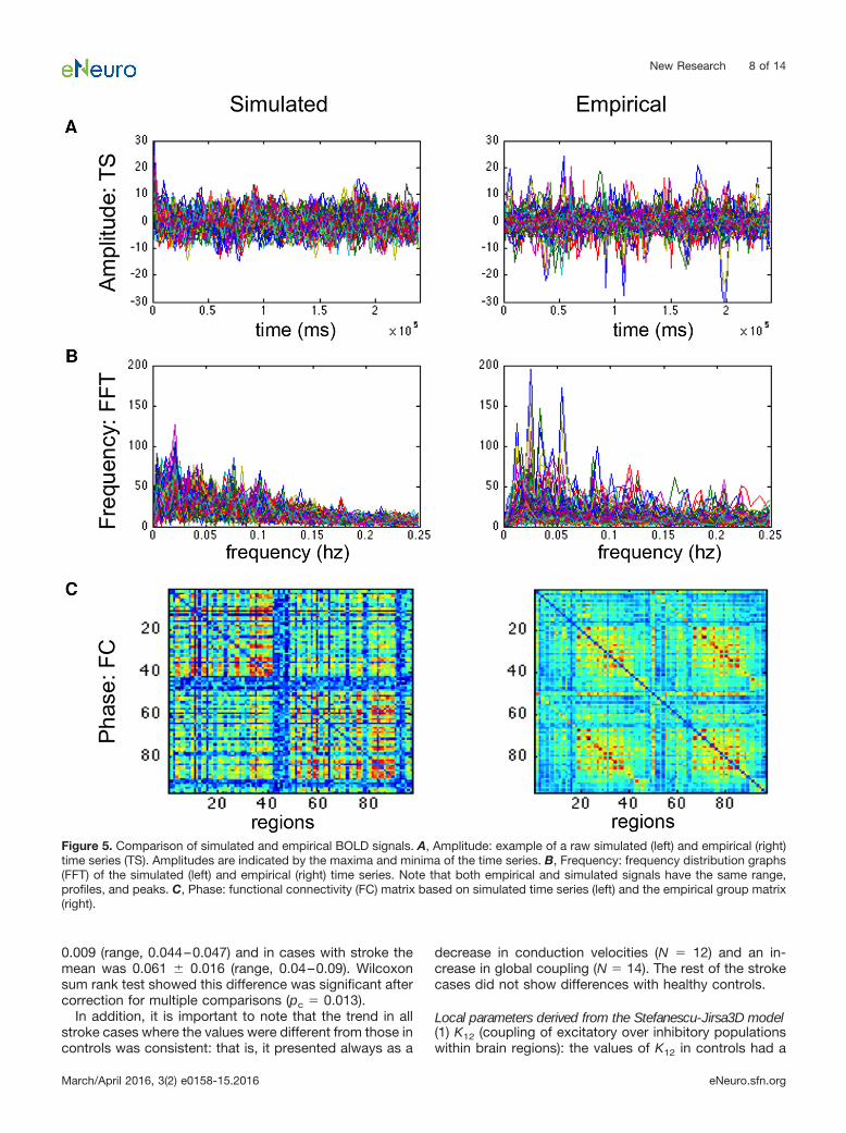
BOLD simulations generated with TVB correlatedwith the empirical BOLD responsesThe frequency spectrums of the simulated and the empir-ical BOLD responses had similar ranges (0–0.25 Hz) andmean peak (empirical � 0.05 � 0.035 Hz; simulated �0.03 � 0.023 Hz; Fig. 5). Although the mean amplitudeswere similar (empirical � 8.15; simulated � 9.49), therange of values was wider in the empirical signals (0.17–87.43) than those found in the simulated BOLD (3.79–22.64). The relative phases of the regions within simulatedand empirical time series were similar as assessed by themean correlation coefficient between their respectivefunctional connectivity matrices (mean � 0.27�0.02; pb �0. 9e-12 Fisher Z-transformation). These validated simu-lations provided us with specific parameter values at boththe global and the local levels associated with healthycontrol subjects and after stroke.

Stroke was associated with reliable changes inglobal and local parametersAlthough qualitative in nature, the color-coded graphicrepresentation of the variance distribution done as part ofthe parameter space exploration (Table 3; Fig. 3) providesa glimpse into differences of combined values for the twoglobal parameters: global coupling (x-axis) and conduc-

tion velocity (y-axis) in healthy controls and in strokesubjects, with warm colors representing higher variance.These explorations demonstrated at this early stage ofanalysis that the range of optimal parameter values (hotcolors) in controls had similar topology of the distributionof variance, as well as concrete values. In contrast, strokecases displayed high variations in both topology andvalues, where although some had similar distribution pat-terns as the healthy controls, others had scattered, frag-mented patterns. Similar observations were found withrespect to local parameters (Table 4).

Numerically, differences in parameter values betweenhealthy controls and the stroke cohort are as follows:

Global parameters(1) Conduction velocity: the range of modeled conductionvelocities obtained via TVB in healthy controls rangedfrom 45 to 90 m/s with a mean of 62 � 10 m/s. In contrast,the conduction velocities in stroke subjects had a rangebetween 12 and 80 m/s with a mean of 46 � 21 m/s.Comparison between the two groups with Wilcoxon ranksum test (pc � 0.05) was marginally significant after cor-rection for multiple comparisons.(2) Global coupling (res-cale factor of incoming activity linking global with localdynamics): in healthy controls, the mean was 0.053 �

Figure 4. Weights of structural connections in stroke and healthy controls. A, Structural connectivity matrices in a healthy control (left)and one individual with stroke (right). Dark blue denotes absence of connections while hotter colors indicate stronger weights. B,Frequency distribution of weight of connections in healthy controls (orange bars) and stroke (blue bars).

New Research 7 of 14

March/April 2016, 3(2) e0158-15.2016 eNeuro.sfn.org

0.009 (range, 0.044–0.047) and in cases with stroke themean was 0.061 � 0.016 (range, 0.04–0.09). Wilcoxonsum rank test showed this difference was significant aftercorrection for multiple comparisons (pc � 0.013).

In addition, it is important to note that the trend in allstroke cases where the values were different from those incontrols was consistent: that is, it presented always as a

decrease in conduction velocities (N � 12) and an in-crease in global coupling (N � 14). The rest of the strokecases did not show differences with healthy controls.

Local parameters derived from the Stefanescu-Jirsa3D model(1) K12 (coupling of excitatory over inhibitory populationswithin brain regions): the values of K12 in controls had a

Figure 5. Comparison of simulated and empirical BOLD signals. A, Amplitude: example of a raw simulated (left) and empirical (right)time series (TS). Amplitudes are indicated by the maxima and minima of the time series. B, Frequency: frequency distribution graphs(FFT) of the simulated (left) and empirical (right) time series. Note that both empirical and simulated signals have the same range,profiles, and peaks. C, Phase: functional connectivity (FC) matrix based on simulated time series (left) and the empirical group matrix(right).

New Research 8 of 14

March/April 2016, 3(2) e0158-15.2016 eNeuro.sfn.org

mean of 0.49 � 0.338 (range, 0.12–0.55) and in stroke themean was 0.369 � 0.257 (range, 0.1–0.8). Statisticalcomparison between the two groups resulted in pc �0.17.

(2) K21 (coupling of inhibitory over excitatory popula-tions): this variable (control mean � 0.804 � 0.17; range,0.3–0.9) was significantly reduced in the stroke group(mean � 0.674 � 0.302; range, 0.1–0.9; pc � 0.01).

(3) K11 (influence between excitatory populations):the values of K11 in controls had a mean of 0.833 �0.142 (range, 0.6 – 0.95) and in stroke cases had a meanof 0.613 � 0.301 (range, 0.1– 0.99). Comparison be-tween the two groups with Wilcoxon sum rank test gavepc � 0.1.

In summary, compared to values in healthy controls,there was a higher global coupling and a decrease of localinhibitory dynamics represented by the local parameterK21 along with a trend toward a reduction of conductionvelocity.

Global and local parameters were correlated withclinical phenotypeMultiple linear regression analysis to establish a relation-ship between modeling parameters and some clinical

metrics did not show a correlation. The following clinicalelements were considered in this preliminary assessment:stroke phenotype (size, location, time after stroke, side ofstroke), depression, patient demographics (age, sex), andseverity of impairment.

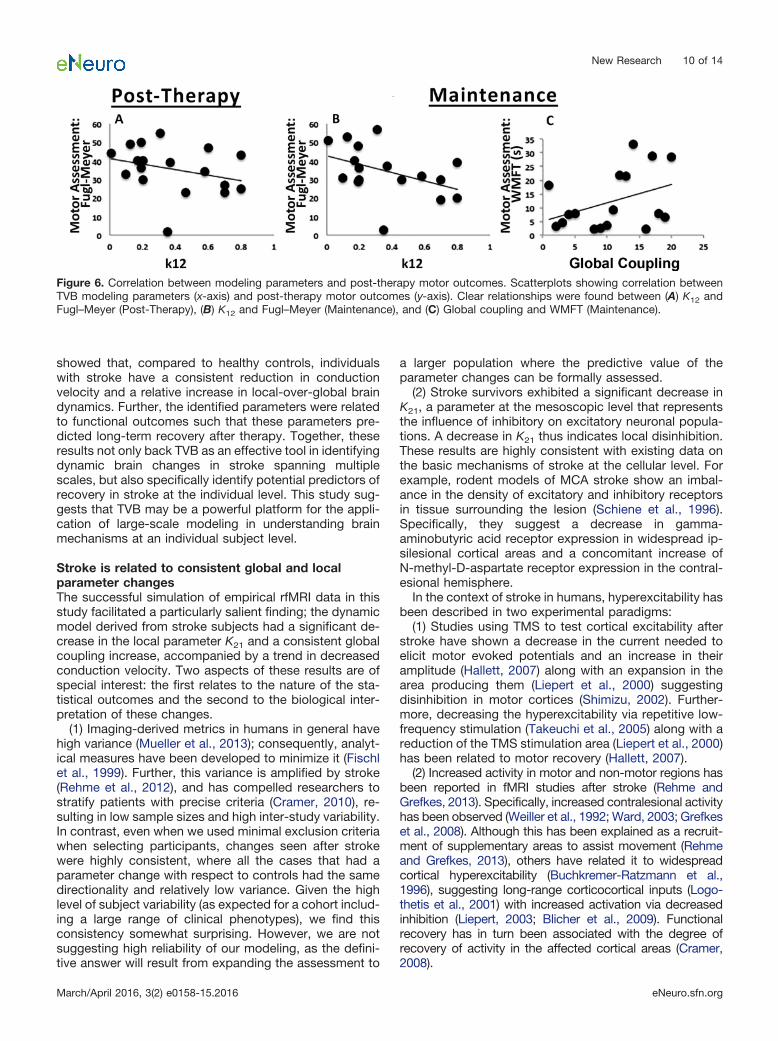
Next, we assessed the relationship between parametervalues with recovery from stroke immediately after ther-apy and after 1 year (maintenance) using a multiple linearregression. This analysis showed a negative relationshipbetween K12 and Fugl–Meyer scores both post-therapy (t��2.386; pd �0.038) and at maintenance 1 year later (t��3.824; pd �0.005). In addition, global coupling had apositive relationship with the Wolf Motor Function Test (t�2.461; pd �0.039) at maintenance. Thus, these two pa-rameters derived from modeling based on pre-therapyconditions were related to long-term motor gains ratherthan the physical features of the stroke or the patient’sdemographics (Fig. 6).

DiscussionThe main result of the study showed that the simulation ofBOLD signals using TVB in stroke enables the identifica-tion of key changes associated with large-scale neuraldynamics in individual patients. Overall, our results

Table 3. Summary of long-range and local parameters used in TVB to simulate BOLD time series in healthy controls andindividuals with stroke

Group Variable Range Mean SDWilcoxonrank sum, p

Control Global variables:Global coupling 0.044–0.047 0.053 0.009Conduction velocity 45–90 61.9 9.9Model variables:K12 0.12–0.55 0.49 0.338K21 0.3–0.9 0.804 0.17K11 0.6–0.95 0.833 0.142

Stroke Global variables:Global coupling 0.04–0.09 0.061 0.016 0.013Conduction velocity 12–80 46 21 0.05Model variables:K12 0.1–0.8 0.369 0.257 0.17K21 0.1–0.9 0.674 0.302 0.01K11 0.1–0.99 0.613 0.301 0.1

Table 4. Statistical table

Comparison of interest Data structure Type of test pa Weights of connections: stroke vs control Normal �Kolmogorov–Smirnov test 0.42b Pearson’s correlation coefficients: simulated vs

empirical functional connectivity matricesNormal after

Z-transformationt test 0.9e-12

c TVB parameters: stroke vs control Control: non-normalStroke: normal

Wilcoxon rank sum test Conduction Velocity: 0.05Global Coupling: 0.013K12: 0.17K21: 0.01K11: 0.1

d Regression: TVB parameters with subjectdemographics, lesion characteristicsand recovery

Normal Multiple linear regression Post-therapy:K12, Fugl–Meyer: 0.038Maintenance:K12, Fugl–Meyer: 0.005Global coupling, WMFT: 0.039

p, Probability resulting from the Wilcoxon sum rank test comparing parameter values between the two groups.

New Research 9 of 14

March/April 2016, 3(2) e0158-15.2016 eNeuro.sfn.org

showed that, compared to healthy controls, individualswith stroke have a consistent reduction in conductionvelocity and a relative increase in local-over-global braindynamics. Further, the identified parameters were relatedto functional outcomes such that these parameters pre-dicted long-term recovery after therapy. Together, theseresults not only back TVB as an effective tool in identifyingdynamic brain changes in stroke spanning multiplescales, but also specifically identify potential predictors ofrecovery in stroke at the individual level. This study sug-gests that TVB may be a powerful platform for the appli-cation of large-scale modeling in understanding brainmechanisms at an individual subject level.

Stroke is related to consistent global and localparameter changesThe successful simulation of empirical rfMRI data in thisstudy facilitated a particularly salient finding; the dynamicmodel derived from stroke subjects had a significant de-crease in the local parameter K21 and a consistent globalcoupling increase, accompanied by a trend in decreasedconduction velocity. Two aspects of these results are ofspecial interest: the first relates to the nature of the sta-tistical outcomes and the second to the biological inter-pretation of these changes.

(1) Imaging-derived metrics in humans in general havehigh variance (Mueller et al., 2013); consequently, analyt-ical measures have been developed to minimize it (Fischlet al., 1999). Further, this variance is amplified by stroke(Rehme et al., 2012), and has compelled researchers tostratify patients with precise criteria (Cramer, 2010), re-sulting in low sample sizes and high inter-study variability.In contrast, even when we used minimal exclusion criteriawhen selecting participants, changes seen after strokewere highly consistent, where all the cases that had aparameter change with respect to controls had the samedirectionality and relatively low variance. Given the highlevel of subject variability (as expected for a cohort includ-ing a large range of clinical phenotypes), we find thisconsistency somewhat surprising. However, we are notsuggesting high reliability of our modeling, as the defini-tive answer will result from expanding the assessment to

a larger population where the predictive value of theparameter changes can be formally assessed.

(2) Stroke survivors exhibited a significant decrease inK21, a parameter at the mesoscopic level that representsthe influence of inhibitory on excitatory neuronal popula-tions. A decrease in K21 thus indicates local disinhibition.These results are highly consistent with existing data onthe basic mechanisms of stroke at the cellular level. Forexample, rodent models of MCA stroke show an imbal-ance in the density of excitatory and inhibitory receptorsin tissue surrounding the lesion (Schiene et al., 1996).Specifically, they suggest a decrease in gamma-aminobutyric acid receptor expression in widespread ip-silesional cortical areas and a concomitant increase ofN-methyl-D-aspartate receptor expression in the contral-esional hemisphere.

In the context of stroke in humans, hyperexcitability hasbeen described in two experimental paradigms:

(1) Studies using TMS to test cortical excitability afterstroke have shown a decrease in the current needed toelicit motor evoked potentials and an increase in theiramplitude (Hallett, 2007) along with an expansion in thearea producing them (Liepert et al., 2000) suggestingdisinhibition in motor cortices (Shimizu, 2002). Further-more, decreasing the hyperexcitability via repetitive low-frequency stimulation (Takeuchi et al., 2005) along with areduction of the TMS stimulation area (Liepert et al., 2000)has been related to motor recovery (Hallett, 2007).

(2) Increased activity in motor and non-motor regions hasbeen reported in fMRI studies after stroke (Rehme andGrefkes, 2013). Specifically, increased contralesional activityhas been observed (Weiller et al., 1992; Ward, 2003; Grefkeset al., 2008). Although this has been explained as a recruit-ment of supplementary areas to assist movement (Rehmeand Grefkes, 2013), others have related it to widespreadcortical hyperexcitability (Buchkremer-Ratzmann et al.,1996), suggesting long-range corticocortical inputs (Logo-thetis et al., 2001) with increased activation via decreasedinhibition (Liepert, 2003; Blicher et al., 2009). Functionalrecovery has in turn been associated with the degree ofrecovery of activity in the affected cortical areas (Cramer,2008).

Figure 6. Correlation between modeling parameters and post-therapy motor outcomes. Scatterplots showing correlation betweenTVB modeling parameters (x-axis) and post-therapy motor outcomes (y-axis). Clear relationships were found between (A) K12 andFugl–Meyer (Post-Therapy), (B) K12 and Fugl–Meyer (Maintenance), and (C) Global coupling and WMFT (Maintenance).

New Research 10 of 14

March/April 2016, 3(2) e0158-15.2016 eNeuro.sfn.org

Complementing the above, our results show a corre-spondence between local and global levels. Indeed, thereduction in local inhibitory influence over excitatory pop-ulations was accompanied by an increase in global cou-pling, reflecting an imbalance after stroke between globaland local brain dynamics, favoring the latter. That is, localdynamics exert a stronger influence than global dynamicsfollowing stroke. In this case, the imbalance could beexacerbated by the decrease in conduction velocity. In-terestingly, this imbalance has also recently been mod-eled in other brain diseases. For example, early stages ofschizophrenia have been associated with a breakdown oflocal dynamics occurring prior to the disruption of globaldynamics occurring later on in disease progression (Ru-binov et al., 2009; van den Berg et al., 2012).

A particularly interesting finding was the trend associ-ated with a decrease in conduction velocity in individualswith stroke, as it has previously been described throughmeasurements of central motor conduction times (CM-CTs) via transcranial magnetic stimulation (TMS) in theprimary motor cortex. Immediately following stroke,CMCT decreases and correlates with functional measures(Abbruzzese et al., 1991; Pennisi, 2002) tending toward anincomplete normalization over the long-term (Heald et al.,1993). That being said, there is a paucity of information ondecreased conduction velocity on corticocortical connec-tions. The bulk of knowledge derives from studies inrodents showing structural changes to axons and oligo-dendrocytes in the primary lesion and the ischemic pen-umbra (Rosenzweig and Carmichael, 2015). In addition,although some degree of remyelination occurs in therecovery phase, the process is often arrested before com-pletion (Syed et al., 2008). In human autopsy samples,there is an increase in nodal and paranodal lengths adja-cent to lacunar lesions (Hinman et al., 2015), which maylead to decreased conduction velocities (Rasband, 2011).Our results thus provide direction for future animal stud-ies, exemplifying the translational nature of TVB findings.

TVB thus appears to be effective at modeling brainactivity in healthy brains and those impacted by diseaseprocesses, and has the novel capability of studying braindynamics at multiple scales, including at a level that hasthus far only been available via animal models or surro-gate neuroimaging markers in humans. Applying thismethod of modeling, which is tied directly to biologicalmechanisms, to existing large datasets opens up thepossibility to experiment with expanded models of brainstates, including a myriad of diseases and their potentialtreatments.

Potential predictors of motor recovery after strokeOur results demonstrated that local (K12) and global(global coupling) parameters, derived from pre-therapyconditions, were significantly correlated with motor gainspost-therapy and at maintenance. Furthermore, both pa-rameters point in the same direction, as poor recoverywas associated with an increase in local excitatory influ-ences and with an emphasis on local dynamics, whereasvalues closer to controls correlated with better recovery.

Interestingly, TVB parameters in stroke did not cor-relate with severity of disease at the pre-stroke timepoint, even though the structural connectivity matrixused in the modeling coincided with this time point. Inaddition, other physical features of the stroke (size,location) or patient demographics (sex, age) did notcorrelate with the modeled parameters. Finally, neitherlesion characteristics nor patient demographics corre-lated with recovery, highlighting the unique predictivepotential of these parameters.

The question then becomes to what extent these pa-rameter estimates can be used as predictors of recoveryat the individual patient level. Although a cross-validationapproach using the current dataset could serve to answerthis question, a new and larger stroke cohort is ideal inobtaining estimates of the sensitivity and the specificity ofour markers, due to high variance in stroke. However,there is clear value of our observations even with thislimitation. At present, biomarkers for stroke recovery havebeen limited by the use of “substitute or surrogate” mea-sures derived from brain imaging or electrophysiology,mainly due to the inability to measure in vivo more idealbasic elements, ie, at molecular or cellular levels (Burkeand Cramer, 2013). Indeed, such elements may be ob-served more closely in animal models, but are difficult totranslate to humans due to the limited homology betweenspecies. Specifically, the Stefanescu-Jirsa 3D model usedin this study evolved from the mesoscopic level Hind-marsh–Rose model. The Hindmarsh–Rose model itself isrooted in the principles of the Hodgkin–Huxley neuronequations, in addition to dynamics based on burstingneurons found in invertebrate circuitry (Hindmarsh andRose, 1984). Further, the neural behaviors described bythe Hindmarsh–Rose model have been biologically veri-fied in other animal models (Selverston and Ayers, 2006;Gu, 2013). Therefore, although any model of the me-soscale does not encompass the complexity of brainprocesses at the cellular level, there is likely emergence ofbehavior from the cellular level to the mesoscopic level,exhibiting deterministic behavior that can be modeled andalso observed in vivo.

That is, the transition between the macroscopic andmicroscopic level is represented by population dynamicsat the mesoscopic level (Mitra, 2014). From this, onecould conclude that the path toward basic biomarkersshould include the intermediate mesoscopic level. Indeed,TVB allows one not only to estimate parameters at thatlevel but also to link it to the macroscopic global whole-brain level. TVB is not unique in considering biophysicalparameters as exemplified by inference models basedon DCM (Moran et al., 2011). Basically, there are noconceptual differences in the inferential goals betweenTVB and DCM but they do differ in the detailed me-chanics. For example, whereas TVB develops themodel at the level of large-scale networks, DCM fo-cuses on portions of these networks. Second, andperhaps the key contrast is that whereas DCM fits theparameter of the model but does not generate data,TVB uses the model to generate data, making these twoapproaches highly complementary.

New Research 11 of 14

March/April 2016, 3(2) e0158-15.2016 eNeuro.sfn.org

An interesting and unique aspect of TVB is its highlyindividualized approach, as parameter estimates are de-rived from individualized structural connectivity matricesobtained from each subject, and hence, it can provide thefirst step to customize individual therapeutic interven-tions. For example, our ongoing work is beginning to testpotential “virtual interventions” by modifying specific pa-rameters changed after stroke and determining the de-gree of restoration of brain dynamics on each strokepatient.

A second ability of this modeling approach is to use themodel of an individual patient’s brain connectivity that canbe objectively measured and evaluated as an indicator ofnormal biological processes (such as, resting state activ-ity, rsfMRI), pathogenic processes, or pharmacologicresponses to therapeutic intervention (Biomarkers Defini-tions Working Group, 2001). Dynamics of rsfMRI arehighly nonstationary (Allen et al., 2014) and existing met-rics, including the direct correlation between functionaland structural connectivity, are so far incapable of ad-dressing this issue satisfactorily (Goni, 2014). A number ofstudies have therefore used generative modeling to parsethe relationship between structural and functional con-nectivity. A recent study (Andersen et al., 2014) demon-strated that the fusion of TVB-like network modeling withstructural neuroimaging explains the nonstationary dy-namics observed in rsfMRI. Thus, we propose a concep-tual paradigm shift, in which the dynamic model shifts thenonstationary functional data from imaging at the meso-scopic scale to a more deterministic set of coefficients ina brain model. In other words, complex dynamics cannotbe captured by stationary imaging analyses, but can begenerated by a data-constrained mechanistic model ofbrain- circuit dynamics, as seen in the generative model-ing approach detailed in stroke (Brodersen et al., 2011).Thus, the mathematical model could be seen as a com-pact generator of dynamics-based biomarkers, or even asthe biomarker itself. The primary benefit, as we demon-strated here, is that it becomes easier to understanddisease mechanisms by evaluating the coefficients of themodel.

Of note, the approach used in this study to validatethe simulated time series was to compare frequency,amplitude, and phase of the simulated and empiricalsignals. After the refinement of the TVB models, futurestudies will incorporate a larger variety of multidimen-sional analyses, particularly with respect to temporalvariability in resting state signals. Furthermore, the cur-rent study determined optimal values of local parame-ters applied to all brain regions. Future studies willfocus on local parameters for subsets of brain regions,eg, changing parameters of nodes within and/or arounda stroke lesion to determine how this impacts the re-sultant simulated brain activity. We also note that thetranslational power of our findings depends upon thereproducibility of parameters for a given brain state, theanswer for which will emerge with expanded applica-tion of TVB to other cohorts. The results from this studythus confirm that TVB allows the assessment of bio-physical variables previously unattainable in human

studies. This method provides a potentially importantand novel application of large-scale modeling, in whichwe can probe brain dynamics and biomarkers on anindividual level. Therefore, The Virtual Brain has thepotential to become an important step toward the de-velopment of individualized medicine in stroke.

ReferencesAbbruzzese G, Morena M, Dall’Agata D, Abbruzzese M, Favale E

(1991) Motor evoked potentials (MEPs) in lacunar syndromes.Electroencephalogr Clin Neurophysiol 81:202–208. Medline

Allen EA, Damaraju E, Plis SM, Erhardt EB, Eichele T, Calhoun VD(2014) Tracking whole-brain connectivity dynamics in the restingstate. Cereb Cortex 24:663–676. CrossRef Medline

Andersen KW, Madsen KH, Siebner HR, Schmidt MN, Mørup M,Hansen LK (2014) Non-parametric Bayesian graph models revealcommunity structure in resting state fMRI. Neuroimage 100:301–315. CrossRef Medline

Avants BB, Tustison NJ, Song G, Cook PA, Klein A, Gee JC (2011) Areproducible evaluation of ANTs similarity metric performance inbrain image registration. Neuroimage 54:2033–2044. CrossRefMedline

van den Berg D, Gong P, Breakspear M, van Leeuwen C (2012)Fragmentation: loss of global coherence or breakdown of modu-larity in functional brain architecture? Front Syst Neurosci 6:20.CrossRef Medline

Blicher JU, Jakobsen J, Andersen G, Nielsen JF (2009) Corticalexcitability in chronic stroke and modulation by training: a TMSstudy. Neurorehabil Neural Repair 23:486–493. CrossRef Medline

Boynton GM, Engel SA, Glover GH, Heeger DJ (1996) Linear systemsanalysis of functional magnetic resonance imaging in human V1. JNeurosci 16:4207–4221. Medline

Breakspear M, Jirsa VK (2007) Neuronal dynamics and brain con-nectivity. In: Handbook of brain connectivity (Jirsa VK, McintoshAR, eds), pp 3–64. Berlin: Springer.

Brodersen KH, Schofield TM, Leff AP, Ong CS, Lomakina EI, Buh-mann JM, Stephan KE (2011) Generative embedding for model-based classification of fMRI data. PLoS Comput Biol 7:e1002079.CrossRef Medline

Buchkremer-Ratzmann I, August M, Hagemann G, Witte OW (1996)Electrophysiological transcortical diaschisis after cortical photo-thrombosis in rat brain. Stroke 27:1105–1109; discussion 1109–1111. CrossRef

Burke E, Cramer SC (2013) Biomarkers and predictors of restorativetherapy effects after stroke. Curr Neurol Neurosci Rep 13:329.CrossRef Medline

Carmichael ST (2012) Brain excitability in stroke: the yin and yang ofstroke progression. Arch Neurol 69:161–167. CrossRef Medline

Cox RW (1996) AFNI: software for analysis and visualization offunctional magnetic resonance neuroimages. Comput Biomed Res29:162–173. CrossRef

Cox RW, Jesmanowicz A (1999) Real-time 3D image registration forfunctional MRI. Magn Reson Med 42:1014–1018. Medline

Cramer SC (2008) Repairing the human brain after stroke: I. Mech-anisms of spontaneous recovery. Ann Neurol 63:272–287. Cross-Ref Medline

Cramer SC (2010) Stratifying patients with stroke in trials that targetbrain repair. Stroke 41:S114–S116. CrossRef Medline

Deco G, Senden M, Jirsa V (2012) How anatomy shapes dynamics:a semi-analytical study of the brain at rest by a simple spin model.Front Comput Neurosci 6:68. CrossRef

Van Essen DC (2004) Surface-based approaches to spatial localiza-tion and registration in primate cerebral cortex. Neuroimage 23:S97–S107. CrossRef

Van Essen DC (2005) A population-average, landmark- and surface-based (PALS) atlas of human cerebral cortex. Neuroimage 28:635–662. CrossRef

New Research 12 of 14

March/April 2016, 3(2) e0158-15.2016 eNeuro.sfn.org

Van Essen DC, Dierker DL (2007) Surface-based and probabilisticatlases of primate cerebral cortex. Neuron 56:209–225. CrossRefMedline

Fischl B, Sereno MI, Tootell RB, Dale AM (1999) High-resolutionintersubject averaging and a coordinate system for the corticalsurface. Hum Brain Mapp 8:272–284. CrossRef

Go AS, Mozaffarian D, Roger VL, Benjamin EJ, Berry JD, Blaha MJ,Dai S, Ford ES, Fox CS, Franco S, Fullerton HJ, Gillespie C,Hailpern SM, Heit JA, Howard VJ, Huffman MD, Judd SE, KisselaBM, Kittner SJ, Lackland DT, et al. (2014) Exectutive summary:heart disease and stroke statistics—2014 update: a report fromthe American Heart Association. Circulation 129:399–410. Cross-Ref

Goni J (2014) Resting-brain functional connectivity predicted byanalytic measures of network communication. Proc Natl Acad SciU S A 111:833-838. CrossRef

Grefkes C, Nowak DA, Eickhoff SB, Dafotakis M, Küst J, Karbe H,Fink GR (2008) Cortical connectivity after subcortical stroke as-sessed with functional magnetic resonance imaging. Ann Neurol63:236–246. CrossRef

Biomarkers Definitions Working Group (2001) Biomarkers and sur-rogate endpoints: preferred definitions and conceptual framework.Clin Pharmacol Ther 69:89–95. CrossRef

Gu H (2013) Biological experimental observations of an unnoticedchaos as simulated by the Hindmarsh-Rose model. PLoS One8:e81759. CrossRef Medline

Hallett M (2007) Transcranial magnetic stimulation: a primer. Neuron55:187–199. CrossRef Medline

Heald A, Bates D, Cartlidge NE, French JM, Miller S (1993) Longitu-dinal study of central motor conduction time following stroke: I.Natural history of central motor conduction. Brain 116:1355–1370.CrossRef

Hindmarsh JL, Rose RM (1984) A model of neuronal bursting usingthree coupled first order differential equations. Proc R Soc B BiolSci 221:87–102. Medline

Hinman JD, Lee MD, Tung S, Vinters HV, Carmichael ST (2015)Molecular disorganization of axons adjacent to human lacunarinfarcts. Brain 138:736–745. CrossRef

Hutchison RM, Womelsdorf T, Allen EA, Bandettini PA, Calhoun VD,Corbetta M, Della Penna S, Duyn JH, Glover GH, Gonzalez-Castillo J, Handwerkere DA, Keilholzk S, Kiviniemil V, LeopoldmDA, de Pasqualeg F, Spornsn O, Waltero M, Chang C (2013)Dynamic functional connectivity: promise, issues, and interpreta-tions. Neuroimage 80:360–378. CrossRef

Jirsa VK, Stefanescu RA (2011) Neural population modes capturebiologically realistic large scale network dynamics. Bull Math Biol73:325–343. CrossRef Medline

Johnstone T, Ores Walsh KS, Greischar LL, Alexander AL, Fox AS,Davidson RJ, Oakes T(2006) Motion correction and the use ofmotion covariates in multiple-subject fMRI analysis. Hum BrainMapp 27:779–788. CrossRef Medline

Leemans A, Jones DK (2009) The B-matrix must be rotated whencorrecting for subject motion in DTI data. Magn Reson Med 61:1336–1349. CrossRef Medline

Liepert J (2003) TMS in stroke. Suppl Clin Neurophysiol 56:368–380.Medline

Liepert J, Graef S, Uhde I, Leidner O, Weiller C (2000) Training-induced changes of motor cortex representations in stroke pa-tients. Acta Neurol Scand 101:321–326. Medline

Logothetis NK, Pauls J, Augath M, Trinath T, Oeltermann A (2001)Neurophysiological investigation of the basis of the fMRI signal.Nature 412:150–157. CrossRef

Lund TE, Madsen KH, Sidaros K, Luo WL, Nichols TE (2006) Non-white noise in fMRI: does modelling have an impact? Neuroimage29:54–66. CrossRef Medline

Mannella R (2002) Integration of stochastic differential equations ona computer. Int J Mod Phys C 13:1177–1194.

Mitra PP (2014) The circuit architecture of whole brains at the meso-scopic scale. Neuron 83:1273–1283. CrossRef Medline

Moran RJ, Symmonds M, Stephan KE, Friston KJ, Dolan RJ (2011)An in vivo assay of synaptic function mediating human cognition.Curr Biol 21:1320–1325. CrossRef Medline

Mueller S, Wang D, Fox MD, Yeo BT, Sepulcre J, Sabuncu MR,Shafee R, Lu J, Liu H (2013) Individual variability in functionalconnectivity architecture of the human brain. Neuron 77:586–595.CrossRef

Nudo RJ (2013) Recovery after brain injury: mechanisms and princi-ples. Front Hum Neurosci 7:887. CrossRef Medline

Pennisi G (2002) Transcranial magnetic stimulation after pure motorstroke. Clin Neurophysiol 113:1536–1543. Medline

Rasband MN (2011) Composition, assembly, and maintenance ofexcitable membrane domains in myelinated axons. Semin Cell DevBiol 22:178–184. CrossRef Medline

Rehme AK, Grefkes C (2013) Cerebral network disorders after stroke:evidence from imaging-based connectivity analyses of active andresting brain states in humans. J Physiol 59:17–31. CrossRef

Rehme AK, Eickhoff SB, Rottschy C, Fink GR, Grefkes C (2012)Activation likelihood estimation meta-analysis of motor-relatedneural activity after stroke. Neuroimage 59:2771–2782. CrossRef

Reiss AP, Wolf SL, Hammel EA, McLeod EL, Williams EA (2012)Constraint-induced movement therapy (CIMT): current perspec-tives and future directions. Stroke Res Treat 2012:159391. Cross-Ref Medline

Ritter P, Schirner M, McIntosh AR, Jirsa V (2013) The virtual brainintegrates computational modelling and multimodal neuroimaging.Brain Connect 49:1–65. CrossRef

Rosenzweig S, Carmichael ST (2015) The axon-glia unit in whitematter stroke: mechanisms of damage and recovery. Brain Res1623:123–134. CrossRef Medline

Roy D, Sigala R, Breakspear M, McIntosh AR, Jirsa VK, Deco G,Ritter P (2014) Using the virtual brain to reveal the role of oscilla-tions and plasticity in shaping brain’s dynamical landscape. BrainConnect. 4:791–811. CrossRef

Rubinov M, Sporns O, van Leeuwen C, Breakspear M (2009) Sym-biotic relationship between brain structure and dynamics. BMCNeurosci 10:55. CrossRef Medline

Sanz Leon P, Knock SA, Woodman MM, Domide L, Mersmann J,McIntosh AR, Jirsa V (2013) The Virtual Brain: a simulator ofprimate brain network dynamics. Front Neuroinform 7:10. Cross-Ref Medline

Sanz-Leon P, Knock SA, Spiegler A, Jirsa VK (2015) Mathematicalframework for large-scale brain network modeling in The VirtualBrain. Neuroimage 111:385–430. CrossRef Medline

Schiene K, Bruehl C, Zilles K, Qü M, Hagemann G, Kraemer M, WitteOW (1996) Neuronal hyperexcitability and reduction of GABAA-receptor expression in the surround of cerebral photothrombosis.J Cereb Blood Flow Metab 16:906–914. Medline

Selverston AI, Ayers J (2006) Oscillations and oscillatory behavior insmall neural circuits. Biol Cybern 95:537–554. CrossRef Medline

Shimizu T (2002) Motor cortical disinhibition in the unaffected hemi-sphere after unilateral cortical stroke. Brain 125:1896–1907. Med-line

Smith SM (2002) Fast robust automated brain extraction. Hum BrainMapp 17:143–155. CrossRef

Solodkin A, Hasson U, Siugzdaite R, Schiel M, Chen EE, Kotter R,Small SL (2010) Virtual brain transplantation (VBT): a method foraccurate image registration and parcellation in large corticalstroke. Arch Ital Biol 148:219–241. Medline

Stefanescu RA, Jirsa VK (2008) A low dimensional description ofglobally coupled heterogeneous neural networks of excitatory andinhibitory neurons. PLoS Comput Biol 4:e1000219. CrossRef Med-line

Syed YA, Baer AS, Lubec G, Hoeger H, Widhalm G, Kotter MR (2008)Inhibition of oligodendrocyte precursor cell differentiation bymyelin-associated proteins. Neurosurg Focus 24:E5. CrossRefMedline

Takeuchi N, Chuma T, Matsuo Y, Watanabe I, Ikoma K (2005)Repetitive transcranial magnetic stimulation of contralesional pri-

New Research 13 of 14

March/April 2016, 3(2) e0158-15.2016 eNeuro.sfn.org

mary motor cortex improves hand function after stroke. Stroke36:2681–2686. CrossRef

Ward NS (2003) Neural correlates of outcome after stroke: a cross-sectional fMRI study. Brain 126:1430–1448. Medline

Weiller C, Chollet F, Friston KJ, Wise RJ, Frackowiak RS (1992)Functional reorganization of the brain in recovery from striatocap-sular infarction in man. Ann Neurol 31:463–472. CrossRef Medline

Zalesky A, Fornito A (2009) A DTI-derived measure of cortico-corticalconnectivity. IEEE Trans Med Imaging 28:1023–1036. CrossRefMedline

Zhang Y, Brady M, Smith S (2001) Segmentation of brain MR imagesthrough a hidden Markov random field model and the expectation-maximization algorithm. IEEE Trans Med Imaging 20:45–57.CrossRef

New Research 14 of 14

March/April 2016, 3(2) e0158-15.2016 eNeuro.sfn.org