Fully coupled, multi-axial, symmetric constitutive laws ...

Journal of the Mechanics and Physics of Solids50 (2002) 127–152

www.elsevier.com/locate/jmps

Fully coupled, multi-axial, symmetric constitutivelaws for polycrystalline ferroelectric ceramics

Chad M. Landis ∗

Department of Mechanical Engineering and Materials Science, MS 321, Rice University,P.O. Box 1892, Houston, TX 77251, USA

Received 10 November 2000; received in revised form 19 February 2001

Abstract

In this paper, a general form for multi-axial constitutive laws for ferroelectric ceramics isconstructed. The foundation of the theory is an assumed form for the Helmholtz free energyof the material. Switching surfaces and associated 3ow rules are postulated in a modi4ed stressand electric 4eld space such that a positive dissipation rate during switching is guaranteed. Theresulting tangent moduli relating increments of stress and electric 4eld to increments of strain andelectric displacement are symmetric since changes in the linear elastic, dielectric and piezoelectricproperties of the material are included in the switching surface. Finally, parameters of the modelare determined for two uncoupled cases, namely non-remanent straining ferroelectrics and purelyferroelastic switching, and then for the fully coupled ferroelectric case. ? 2001 Elsevier ScienceLtd. All rights reserved.

Keywords: A. Electromechanical process; B. Non-linear constitutive behavior; B. Ferroelectric material;C: Hysteresis; Ferroelectric switching

1. Introduction

The need for an accurate yet simple mathematical description of the constitutive be-havior of ferroelectric ceramics is self-evident. The piezoelectric actuator is an exampleof an application where such a constitutive law would be useful. Near an electrode tipin an actuator the electric 4eld and polarization of the material are non-uniform. Pre-diction of the non-uniform 4elds around an electrode tip or possibly a crack tip wouldmost likely require detailed 4nite element calculations. An adequate constitutive lawfor the ferroelectric material is required to perform these calculations.

∗ Tel.: +1-713-348-3609; fax: +1-713-348-5423.E-mail address: [email protected] (C.M. Landis).

0022-5096/01/$ - see front matter ? 2001 Elsevier Science Ltd. All rights reserved.PII: S0022 -5096(01)00021 -7

128 C.M. Landis / J. Mech. Phys. Solids 50 (2002) 127–152

Accurate constitutive laws already exist for ferroelectric ceramics. The most notableis the self-consistent model of Huber et al. (1999). The self-consistent model derivesits accuracy by averaging the behavior of a large number of single crystals that areassumed to change remanent polarization and strain due to domain wall motion oncrystallographically de4ned transformation systems. While this law is able to adequatelyreproduce the multi-axial behavior of ferroelectrics, see Huber and Fleck (2001), it isunfortunately relatively slow to compute. Finite element calculations employing theself-consistent constitutive law would take at least 10 times longer to complete thana constitutive law with only the remanent strain and remanent polarization as internalvariables.

Instead of micromechanically based constitutive laws like the self-consistent consti-tutive law mentioned previously, a phenomenological law with fewer internal variablesis desired. There already exists an abundance of experimental observations with whichsuch a law must be in agreement, Lynch (1996), Fett et al. (1998) and Huber andFleck (2001). Furthermore, complications associated with the non-linear coupling be-tween the states of remanent strain and remanent polarization as well as changes in thelinear piezoelectric properties must be considered. Finally, the phenomena of “lock-up”or polarization=strain saturation must be predicted.

The 4rst part of this work is concerned with developing a general formulation forferroelectric constitutive laws that yield symmetric tangent moduli while allowing forchanges in linear piezoelectric properties during switching. The foundation of these lawsis the Helmholtz free energy approach utilized by Bassiouny et al. (1988a, b), Bassiounyand Maugin (1989a, b) and Cocks and McMeeking (1999). Switching surfaces andassociated 3ow rules for increments of remanent strain and polarization are proposedto ensure that the energy dissipation rate in the material is always non-negative. The4nal results of the model remain abstract, as a number of tensorial parameters are notdetermined by the theory. These parameters are the 4tting parameters of the model andare of course material speci4c.

To make the theory of the 4rst section more concrete, the second part of this workwill be concerned with proposing switching surfaces and hardening moduli to rep-resent actual ferroelectric ceramics. First, a simple form for the dependence of thelinear properties on the material polarization will be proposed and the appropriatederivatives required for the general theory will be given. Thereafter, functional formsfor the switching surfaces and hardening moduli are given for two uncoupled cases,non-remanent straining ferroelectrics and ferroelastic switching. Finally, the fully cou-pled case is presented with coupling terms appearing in both the switching surfaceand hardening moduli. A comparison of the fully coupled theory with the experi-mental measurements of Lynch (1996) and Huber and Fleck (2001) appears to befavorable.

2. Preliminaries

In this section, the equations governing a small deformation, isothermal, ferroelectricboundary value problem will be reviewed. Throughout standard Einstein notation is

C.M. Landis / J. Mech. Phys. Solids 50 (2002) 127–152 129

utilized with summation implied over repeated indices. Consider a volume of ferro-electric material, V , bounded by the surface, S.

Mechanical equilibrium of stresses is given by

�ij; j = −bi in V (2.1)

and

||�ij||nj = −ti on S; (2.2)

where �ij is the Cauchy stress tensor, bi is the body force in the volume, ni is a unitvector normal to the surface directed outward from the volume, ti is the traction appliedby external agencies to the surface and || || denotes a jump (outside minus inside) inthe included quantity.

The in4nitesimal strain–displacement compatibility conditions are

�ij = 12 (ui; j + uj; i); (2.3)

where �ij is the in4nitesimal strain tensor and ui are the components of material dis-placement.

Gauss’ law is written as

Di; i = qv in V (2.4)

and

||Di||ni = qs on S; (2.5)

where Di is the electric displacement, qv is the free charge per unit volume in V andqs is the free charge per unit area residing on S.

Under quasi-static conditions the electric 4eld, Ei, can be written as the gradient ofa potential, �, such that

Ei = −�;i: (2.6)

Finally, the linear piezoelectric constitutive law is given by

�ij − �rij = sE

ijkl�kl + dkijEk ; (2.7)

Di − Pri = dikl�kl + ��

ijEj; (2.8)

where �rij and Pr

i are the remanent strain and polarization, sEijkl is the fourth-order tensor

of elastic compliance measured at constant applied electric 4eld, dkij is the third-ordertensor of piezoelectricity and ��

ij is the second-order tensor of dielectric permittivitymeasured at constant applied stress. The goal of any rate independent ferroelectricconstitutive law is to relate increments of stress and electric 4eld to increments ofstrain and electric displacement such that

�ij = sE; tijkl�kl + dt

kijEk ; (2.9)

Di = dtikl�kl + ��; t

ij Ej; (2.10)

where the superscripted t denotes tangent moduli and the symmetry of the tangentpiezoelectric tensor dt

kij in Eqs. (2.9) and (2.10) has been assumed.


Eqs. (2.1)–(2.10) can be written in weak form as∫V

�u i; jcE; tijklu k; l + �u i; jet

kij�;k + ��; ietiklu k; l − ��; i�

�; tij �; j dV

=∫V

bi�u i − qv�� dV +∫Sti�u i − qs�� dS: (2.11)

Here cE; tijkl, et

kij and ��; tij are related to sE; t

ijkl, dtkij and ��; t

ij through manipulation of Eqs.(2.9) and (2.10). Eq. (2.11) can be used to derive 4nite element equations to solvecomplex boundary value problems. The 4nite element matrix derived from Eq. (2.11)will be symmetric if the tangent constitutive relation is also symmetric, as has beenassumed in Eqs. (2.9)–(2.11). The next section of this paper will be devoted todetermining these tangent moduli.

3. General formulation for ferroelectric switching

This work is concerned with isothermal, rate-independent deformation and polar-ization processes. The extension to rate dependence is discussed in the appendix.Both deviatoric and volumetric remanent straining are allowed. In a fashion similarto Bassiouny et al. (1988a) and Cocks and McMeeking (1999), the Helmholtz freeenergy for the material is introduced as

� = �s(�ij; �rij ; Di; Pr

i ) + �r(�rij ; P

ri ): (3.1)

The reversible or stored part of the free energy is �s and �r represents an additionalcontribution to the free energy associated only with the internal state of the material.It is assumed that the remanent strain and remanent polarization fully characterize theinternal state of the material. Then, assuming linear piezoelectric response the 4rst termin Eq. (3.1) is written as

�s = 12c

Dijkl(�ij − �r

ij)(�kl − �rkl) − hkij(Dk − Pr

k)(�ij − �rij)

+ 12�

�ij(Di − Pr

i )(Dj − Prj): (3.2)

Note that cDijkl, hkij and ��

ij can depend on �rij and Pr

i .The stress and electric 4eld can be derived from the Helmholtz free energy as

�ij =9�9�ij

=9�s

9�ij= cD

ijkl(�kl − �rkl) − hkij(Dk − Pr

k); (3.3)

Ei =9�9Di

=9�s

9Di= −hikl(�kl − �r

kl) + ��ij(Dj − Pr

j): (3.4)


Inversion of Eqs. (2.7) and (2.8) can be used to relate cDijkl, hkij and ��

ij to sEijkl, dkij

and ��ij. Derivatives of �s with respect to �r

ij and Pri are

9�s

9�rij

= −�ij − 12

9sEpqrs

9�rij

�pq�rs − 9dqrs

9�rij

Eq�rs − 12

9��pq

9�rij

EpEq; (3.5)

9�s

9Pri

= −Ei − 12

9sEpqrs

9Pri


9PriEq�rs − 1

2

9��pq

9PriEpEq: (3.6)

Here a Legendre transformation has been used indicating that

12

9cDpqrs

9�rij

(�pq − �rpq)(�rs − �r

rs) −9hqrs

9�rij

(Dq − Prq)(�rs − �r

rs)

+12

9��pq

9�rij

(Dp − Prp)(Dq − Pr

q)

= − 12

9sEpqrs

9�rij


9�rij

Eq�rs − 12

9��pq

9�rij

EpEq = − K�ij: (3.7)

and

12

9cDpqrs

9Pri

(�pq − �rpq)(�rs − �r

rs) −9hqrs

9Pri

(Dq − Prq)(�rs − �r

rs)

+12

9��pq

9Pri

(Dp − Prp)(Dq − Pr

q)

= − 12

9sEpqrs

9Pri


9PriEq�rs − 1

2

9��pq

9PriEpEq = − KEi: (3.8)

Note that Eqs. (3.7) and (3.8) have been used to de4ne K�ij and KEi. Finally the backstress, �B

ij, and back electric 4eld, EBi , are conjugate to �r

ij and Pri such that

�Bij =

9�r

9�rij

(3.9)

and

EBi =

9�r

9Pri: (3.10)


The second law of thermodynamics implies that the dissipation rate, !, for the materialis non-negative, i.e.

! = �ij�ij + EiDi − �

= �ij �rij + EiP

ri ¿ 0; (3.11)

where

�ij = �ij − �Bij + K�ij (3.12)

and

Ei = Ei − EBi + KEi: (3.13)

It is possible to satisfy Eq. (3.11) with separate switching surfaces and 3ow poten-tials; however, a simpler associated 3ow rule is utilized here. Speci4cally, the inequalityof Eq. (3.11) and additionally the electromechanical form of the postulate of maximumplastic dissipation, Drucker (1952), will be satis4ed for any convex yield surface, ",containing the origin in (�ij ; Ei) space with an associated normality condition for the3ow rule. Note that the switching surface does not necessarily enclose the origin instandard stress and electric 4eld space.

During switching the condition

"(�ij ; Ei; �rij ; P

ri ) = 0 (3.14)

must be satis4ed. The increments of remanent strain and polarization are normal to theswitching surface such that

�rij = #

9"9�ij

= #�ij (3.15)

and

Pri = #

9"9Ei

= #Pi: (3.16)

Note that �ij and Pi are de4ned in Eqs. (3.15) and (3.16). No restrictions are placed onthe dimensionality of ". However, if " has dimensions of energy density then �ij andPi have dimensions of strain and polarization, respectively. The plastic multiplier # isgreater than zero during a switching increment and equal to zero during an incrementof linear response. Linear response occurs if the current state in (�ij ; Ei) space iswithin the switching surface or the current state is on the switching surface but theincremented state (�ij + ˙�ij; Ei + ˙Ei) lies within the switching surface.

During switching the consistency condition requires that

" = �ij ˙�ij + Pi˙Ei +

9"9�r

ij�rij +

9"9Pr

iP

ri = 0: (3.17)

To analyze the consequences of Eq. (3.17) a number of tensors are now de4ned

Umijkl =

12

92sEpqrs

9�rij9�r

kl�pq�rs +

92dqrs

9�rij9�r

klEq�rs +

12

92��pq

9�rij9�r

klEpEq; (3.18)


U emkij =

12

92sEpqrs

9Prk9�r

ij�pq�rs +

92dqrs

9Prk9�r

ijEq�rs +

12

92��pq

9Prk9�r

ijEpEq; (3.19)

U eij =

12

92sEpqrs

9Pri 9Pr

j�pq�rs +

92dqrs

9Pri 9Pr

jEq�rs +

12

92��pq

9Pri 9Pr

jEpEq; (3.20)

A��ijkl =

9sEpqij

9�rkl

�pq +9dqij

9�rkl

Eq; (3.21)

A�Pkij =

9sEpqij

9Prk

�pq +9dqij

9PrkEq; (3.22)

AP�kij =

9dkrs

9�rij

�rs +9��

kq

9�rijEq; (3.23)

APPij =

9dirs

9Prj�rs +

9��iq

9PrjEq: (3.24)

Note here that A��ijkl �= A��

klij, A�Pkij �= AP�

kij and APPij �= APP

ji .

Hmijkl =

92�r

9�rij9�r

kl; (3.25)

H emkij =

92�r

9Prk9�r

ij; (3.26)

H eij =

92�r

9Pri 9Pr

j: (3.27)

Hence, the increments of the back stresses and back electric 4elds are related to incre-ments of remanent strain and polarization through the hardening tensors such that

�Bij = Hm

ijkl�rkl + H em

kij Prk ; (3.28)

EBi = H em

ikl �rkl + H e

ijPrj: (3.29)

Eqs. (3.15)–(3.29) can be utilized to determine the plastic multiplier #,

# =1D

(�ij�ij + PiEi) (3.30)


with

D = (Hmijkl − Um

ijkl)�ij �kl + 2(H emkij − U em

kij )Pk �ij

+ (H eij − U e

ij)PiPj − 9"9�r

ij�ij − 9"

9PriPi (3.31)

and

�ij = (�ik�jl + A��ijkl)�kl + A�P

kijPk ; (3.32)

Pi = AP�ikl�kl + (�ij + APP

ij )Pj: (3.33)

The ultimate goal of the constitutive law is to obtain equations in the form of Eqs.(2.9) and (2.10). To accomplish this, Eqs. (2.7) and (2.8) are rewritten as

�ij = sEijkl�kl + dkijEk + �r

ij + A��ijkl�

rkl + A�P

kijPrk ; (3.34)

Di = dikl�kl + ��ijEj + P

ri + AP�

ikl�rkl + APP

ij Prj (3.35)

Then Eqs. (3.15), (3.16) and (3.30) along with the de4nitions of Eqs. (3.32) and (3.33)can be used in Eq. (3.34) and (3.35) to show that

�ij =(sEijkl +

1D

�ij �kl

)�kl +

(dkij +

1D

Pk �ij

)Ek ; (3.36)

Di =(dikl +

1D

Pi�kl

)�kl +

(��ij +

1D

PiPj

)Ej: (3.37)

Eqs. (3.36) and (3.37) are now in the form of Eqs. (2.9) and (2.10) and the ferro-electric constitutive law is complete. Note that the tangent moduli, including the elec-tromechanical cross terms, are symmetric. This feature would not have appeared ifchanges in the linear properties were not accounted for in the description of the switch-ing surface and 3ow rule.

The constitutive law outlined above is based on a consistent thermodynamic formu-lation; however, it is far from being useful for 4nite element calculations. All of therequired inputs to the model are of course material speci4c and it could be argued thatall parameters are measurable. However, direct measurement and determination of thefunctional forms for the switching surface, "(�ij ; Ei; �r

ij ; Pri ), hardening moduli, Hm

ijkl,H em

kij , H eij, and linear properties, sE

ijkl, dkij and ��ij which all can depend on �r

ij and Pri ,

would be a diNcult experimental procedure. As such, it is necessary to gain a deeperunderstanding of the hardening processes and material property changes that occur inferroelectric ceramics in order to make intelligent assumptions about these materialparameters. Ideally such assumptions should reduce the 4tting parameters of the modelfrom a set of tensors to a set of measurable scalar variables.


Section 4 is devoted to determining the remanent polarization and remanent straindependence of the linear properties that are useful for almost all types of polycrystallineferroelectrics. In Section 5 switching surfaces and hardening moduli are proposed formaterials with only the remanent polarization as the internal state variable. This sectionis valid for materials like barium titanate that, under certain conditions, experience littleto no remanent strain. Section 6 develops switching surfaces and hardening moduli forferroelastic switching. For this second uncoupled case, the internal state of the materialis determined only by the remanent strain components. Lastly, Section 7 presents fullycoupled forms of the switching surface and hardening moduli that are able to repro-duce the experimental measurements of Lynch (1996) and Huber and Fleck (2001) toreasonable accuracy.

4. Linear properties

Here functional forms for the linear properties of ferroelectric materials are devel-oped. It is asserted that the following description is the simplest that captures theessential features of piezoelectric property changes during ferroelectric switching. Aferroelectric material is on average unpoled and non-piezoelectric after cooling fromabove the Curie temperature. Polarization and piezoelectricity does of course exist atdomain and possibly even at grain size scales but averaged over a number of grainsthe remanent polarization and piezoelectric eOect vanish. During the application of astrong electric 4eld the polarization and piezoelectric coeNcients of the ferroelectricincrease. A simple form for the linear properties with the highest possible symmetryto describe this increase in the piezoelectricity is

��ij = ��ij; (4.1)

sEijkl =

14'

(�ik�jl + �il�jk) − (2'(1 + ()

�ij�kl; (4.2)

dkij =Pr

P0

[d33nkninj + d31nk)ij +

12d15(ni)jk + nj)ik)

]; (4.3)

where

Pr =√

Pri P

ri ; (4.4)

ni =Pri

Pr (4.5)

and

)ij = �ij − ninj: (4.6)

Here � is the dielectric permittivity of the material measured at constant appliedstress, ' and ( are the shear modulus and Poisson’s ratio measured at constant appliedelectric 4eld and d33; d31 and d15 are the matrix components of the piezoelectricmoduli when the polarization magnitude, Pr , reaches its maximum value of P0. Kamlahand Tsakmakis (1999) and Huber and Fleck (2001) have also used Eq. (4.3) for the


piezoelectric tensor. Notice that the dielectric permittivity and the elastic compliance areassumed to be isotropic and the piezoelectricity is assumed to be transversely isotropicabout an axis of symmetry aligned with the polarization direction ni. Note that otherforms of the elastic and dielectric tensors, such as cD

ijkl and ��ij, will not have isotropic

symmetry but rather transversely isotropic symmetry. Furthermore, the magnitude ofthe piezoelectric eOect is linearly proportional to the magnitude of the polarization.

This description of the linear properties greatly simpli4es many of the equationspresented in Section 3, since any derivatives of the linear properties with respect to theremanent strain components will be zero. Additionally, derivatives of sE

ijkl and ��ij with

respect to the polarization components also vanish. However, the A-tensors introducedin Eqs. (3.22) and (3.24) require the derivatives 9dkij=9Pr

l and (3.20) requires thesecond derivatives 92dkij=9Pr

l9Prm. These derivatives are

9dkij

9Prl

=d33

P0(nkninjnl + ninj)kl + nknj)il + nkni)jl)

+d31

P0()ij)kl + nknl)ij − nink)jl − njnk)il)

+d15

2P0()il)jk + )ik)jl + ninl)jk + njnl)ik − nink)jl − njnk)il − 2ninj)kl);

(4.7)

92dkij

9Prl9Pr

m=

d33

P0Pr (ni)kl)jm + ni)jl)km + nj)il)km + nj)im)kl

+ nk)il)jm + nk)im)jl − 2nkninj)lm)

+d31

P0Pr (2nkninj)lm − ni)kl)jm − ni)jl)km − nj)il)km

− nj)im)kl − nk)il)jm − nk)im)jl)

+d15

2P0Pr (4nkninj)lm − 2ni)kl)jm − 2ni)jl)km − 2nj)im)kl

− 2nj)il)km − 2nk)il)jm − 2nk)im)jl): (4.8)

A complete theory for a given ferroelectric material still requires the speci4cationof the functional forms for the switching surface and hardening moduli. These featureswill be addressed for diOerent cases in the following sections.

5. Non-remanent straining ferroelectrics

This section is devoted to determining the functional forms of the switching sur-face and hardening moduli for non-remanent straining materials. This development haspractical importance for 4ne-grained barium titanate (see Schneider and Heyer, 1999)and any other ferroelectrics, which exhibit virtually linear stress–strain behavior. A


simple form for the yield surface is given and the hardening moduli are determined.The hardening moduli are derived by assuming that the internal state of the materialis uniquely determined by the remanent polarization.

5.1. Switching surface

For the materials considered in this section the remanent strain is always zero.Note that the 3ow rule given by Eq. (3.15) implies that remanent straining occurs ifthe switching surface depends on �ij. Hence, the switching surface for non-remanentstraining materials is of the form, "(Ei; Pr

i ). A simple isotropic form for the switchingsurface is

" = EiEi − E20

=[(

�ij +9djkl

9Pri�kl

)Ej − EB

i

] [(�ij +

9djkl

9Pri�kl

)Ej − EB

i

]− E2

0

= 0: (5.1)

This switching surface is a sphere in Ei space with a radius equal to the coercive4eld, E0.

To this point, the scalar parameters de4ning the model are the elastic constants, 'and (, the dielectric constant, �, the piezoelectric coeNcients, d33; d31 and d15, thelock-up or saturation level of remanent polarization, P0, and the coercive 4eld E0.What remains to complete the model is the determination of the hardening moduli H e

ij.

5.2. Hardening moduli

In Section 5.1 isotropic hardening could be included in the model by having thecoercive 4eld depend on the magnitude of the remanent polarization. However, mea-surements of hysteresis loops on ferroelectrics suggest that a purely kinematic descrip-tion of the hardening is suNcient. The hardening rule must be able to describe thephenomena of lock-up. As suggested by the description of the piezoelectric tensor ithas been implicitly assumed that the magnitude of the remanent polarization cannot begreater than P0. Hence, as the remanent polarization approaches P0 the back electric4eld must increase so that increases in remanent polarization require large incrementsin applied electric 4eld.

As mentioned previously the only internal state variable for the material is the vectorPri . This implies that �r =�P(Pr) since no other invariants exist to describe the internal

state of the material. The back electric 4eld is then

EBi =

9�P

9Pri

=9�P

9Pr

9Pr

9Pri

= EBni (5.2)

with

EB =√

EBi E

Bi =

9�P

9Pr : (5.3)


Fig. 1. (a) D–E hysteresis and (b) �–E butter3y loops derived from the theory presented in Section 5 fornon-remanent straining ferroelectrics.

Eq. (5.2) demonstrates that the back electric 4eld is always in the direction of theremanent polarization (recall that ni =Pr

i =Pr) and its magnitude is uniquely determined

by the magnitude of the remanent polarization. The hardening moduli are given as

H eij =

92�P

9Pri 9Pr

j=

dEB

dPr ninj +EB

Pr )ij: (5.4)

In practice, the function EB(Pr) can be measured during a uniaxial poling test on asample of ferroelectric material and the model for the material would be complete.However, in the spirit of simplicity a functional form for EB(Pr) with two 4ttingparameters is given. This form has been borrowed from Huber and Fleck (2001) whichwas found to 4t uniaxial measurements adequately.

�P =H e

0P20

(me − 1)(me − 2)

(1 − Pr

P0

)2−me

− H e0P0

me − 1Pr ; (5.5)

EB =H e

0P0

me − 1

[(1 − Pr

P0

)1−me

− 1

]; (5.6)

H eij = H e

0

(1 − Pr

P0

)−me

ninj +P0

Pr

H e0

me − 1

[(1 − Pr

P0

)1−me

− 1

])ij: (5.7)

Here two new 4tting parameters, H e0 , the slope of the D–E loop just after switch-

ing commences, and me, the electrical hardening exponent have been introduced. Thisbrings the total number of material constants for the model to 10: '; (; �; d33; d31; d15; P0;E0; H e

0 and me.Figs. 1a and b are plots of the uniaxial electric displacement versus electric 4eld

hysteresis loop and strain versus electric 4eld butter3y loop for a set of normalized


material parameters. These loops bear a resemblance to loops measured on 4ne-grainedbarium titanate, Schneider and Heyer (1999). The multi-axial consequences of thehardening moduli from Eq. (5.7) will be demonstrated after the fully coupled versionof the theory is presented.

6. Ferroelastic switching

Unpoled ferroelectric ceramics are able to exhibit ferroelastic behavior in the absenceof applied electric 4elds. Without the biasing in3uence of an applied electric 4eld or anexisting remanent polarization, the application of stress to a polycrystalline ferroelectricceramic will not cause the material to polarize. However, the ceramic can accumulateremanent strain under the action of the applied stress. This section will be devotedto determining a switching surface and hardening rules that characterize ferroelasticswitching.


The general theory outlined in Section 3 allows for both deviatoric and volumetricremanent straining. However, in ferroelectric ceramics that are not experiencing a phasetransformation, the switching process is volume conserving. Therefore, the switchingsurface will depend only on the deviatoric part of the stress, i.e. " = "(sij) wheresij = �ij − 1

3 �kk�ij. A simple, isotropic switching surface in sij space is a sphere suchthat

" = 32 sij sij − �2

0 = 0: (6.1)

The parameter �0 is the yield stress in uniaxial tension. This form of the switchingsurface follows directly from J2 3ow theory for metal plasticity.


In general, the switching potential for ferroelastic switching, �r ; will depend oninvariants of the remanent strain tensor. The three principal remanent strains can bechosen for these invariants, i.e. �r = ��(�r

I ; �rII; �

rIII): Throughout this section the con-

vention �rI ¿ �r

II ¿ �rIII will be used.

From Eq. (3.9) the back stresses are

�Bij =

9��

9�rij

=9��

9�rI

9�rI

9�rij

+9��

9�rII

9�rII

9�rij

+9��

9�rIII

9�rIII

9�rij;

=9��

9�rIlIi l

Ij +

9��

9�rIIlIIi l

IIj +

9��

9�rIII

lIIIi lIII

j ; (6.2)


where lIi ; lII

i and lIIIi are unit vectors in the directions of the principal strains �r

I ; �rII

and �rIII; respectively. Furthermore, the hardening moduli are given by

Hmijkl =

9��

9�rI,Iijkl +

9��

9�rII,IIijkl +

9��

9�rIII

,IIIijkl

+92��

9�rI 9�r

IlIi l

Ijl

Ikl

Il +

92��

9�rII9�r

IIlIIi l

IIj l

IIk l

IIl +

92��

9�rIII9�r

IIIlIIIi lIII

j lIIIk lIII

l

+92��

9�rI9�r

II(lI

i lIjl

IIk l

IIl + lII

i lIIj l

Ikl

Il) +

92��

9�rII9�r

III(lII

i lIIj l

IIIk lIII

l + lIIIi lIII

j lIIk l

IIl )

+92��

9�rI9�r

III(lI

i lIjl

IIIk lIII

l + lIIIi lIII

j lIkl

Il); (6.3)

where

,Kijkl =

92�rK

9�rij 9�r

kl=

99�r

kl(lK

i lKj ): (6.4)

The sub=superscript K can take on the values I, II or III. Here summation is not impliedover the repeated K. At this point the functional form for �� and eNcient methods forcomputing the principal directions and the appropriate derivatives are required.

To compute the principal directions and their derivatives it is noted that the principalremanent strains can be written as

�rK = I1 + J2fK(J3=J2); (6.5)

where

I1 = 13 �

rkk ; (6.6)

J2 = ( 23e

rije

rij)

1=2; (6.7)

J3 = ( 43e

rije

rjke

rki)

1=3; (6.8)

erij = �r

ij − 13 �

rkk�ij; (6.9)

fI = cos(/3

); (6.10)

fII = − 12 cos

(/3

)+

√3

2 sin(/3

); (6.11)

fIII = − 12 cos

(/3

)− √3

2 sin(/3

)(6.12)

and

/ = arccos

[(J3

J2

)3]: (6.13)


DiOerentiation of Eq. (6.5) implies that

9�rK

9�Rij

=13�ij +

23

(fK − J3

J2f′

K

)erij

J2+

43f′

K

J 23

(erike

rkj −

12J 2

2 �ij

)= lK

i lKj (6.14)

and

,Kijkl = �ij�kl

[49J 3

2

J 43f′′

K − 29

1J2

(fK − J3

J2f′

K

)− 8

9J 4

2

J 53f′

K

]

+ �ik�jl

[23

1J2

(fK − J3

J2f′

K

)]

+ (�ijerkl + �kler

ij)[

49

1J2J3

f′′K − 8

91J 2

3f′

K

]

+ (�ikerjl + �jler

ik)[

43

1J 2

3f′

K

]

+ (�ijerkme

rml + �kler

imermj)[

169

J 22

J 53f′

K − 89J2

J 43f′′

K

]

+ erije

rkl

[49J 2

3

J 52f′′

K − 49

1J 3

2

(fK − J3

J2f′

K

)]

+ (erije

rkme

rml + er

imermje

rkl)[−8

91

J 32 J3

f′′K

]

+ erime

rmje

rkne

rnl

[169

1J2J 4

3f′′

K − 329

1J 5

3f′

K

]; (6.15)

where f′K is dfK=d(J3=J2) and f′′

K is d2fK=d(J3=J2)2. Other methods may be usedto determine the derivatives listed in Eqs. (6.14) and (6.15); however, the methoddescribed lends itself to implementation on the computer.

Finally, a functional form for the potential �� is required. Landis and McMeeking(1999) and Huber and Fleck (2001) have already discussed lock-up conditions for fer-roelastic switching. The condition proposed by these researchers is that lock-up occurswhen the minimum principal strain approaches a characteristic value of −�0. Hence, thepotential must increase dramatically as the minimum principal strain approaches −�0.This is a rather simple condition for lock-up, but it is able to account for the asymme-try in the tension versus compressive remanent straining behavior seen in ferroelectrics(Fett et al., 1998).

Along with the lock-up conditions, certain symmetries must exist in ��. For example,for axisymmetric states of remanent strain the derivatives of �� with respect to theremanent strain components must lead to an axisymmetric back stress tensor. Onemethod to enforce such symmetry is to assume that �� is separable into the form

��(�rI ; �

rII; �

rIII) = (�r

I) + (�rII) + (�r

III): (6.16)


Fig. 2. A stress versus strain hysteresis loop derived from the theory presented in Section 6 for ferroelasticswitching.

Under this assumption, the function (�rK) can be determined from a measured, uniaxial

stress–strain hysteresis loop. Since the potential �r is not used directly in the theory, itis suNcient to specify only ′(�r

K). In the same spirit as Section 4:3, a simple functional

form for ′(�r

K) that satis4es the lock-up conditions is

′(�rK) =

2mtH�

0 �(mc+mt )0 �r

K

(�0 + �rK)mc (2�0 − �r

K)mt ; (6.17)

where H�0 is the hardening modulus at the onset of ferroelastic switching, �0 is the

magnitude of the compressive lock-up strain, mc is the compressive hardening expo-nent and mt is the tensile hardening exponent. To determine the hardening tensor, thederivative ′′(�r

K) can be easily obtained from Eq. (6.17). Two hardening exponents,mc and mt , are introduced to allow for a better 4t to the anisotropy in the tensileversus compressive behavior for a given material, see Fett et al. (1998). Note that inthe limits of H�

0 → 0; mc → ∞ and mt → ∞ the model of this section is equiva-lent to the wall type lock-up model of Landis and McMeeking (1999). Finally, thismodel for ferroelastic switching requires 7 material constants, '; (; �0; �0; H�

0 ; mc and mt .

Fig. 2 is a plot of a stress versus strain hysteresis loop predicted by the theory outlinedin this section for a normalized set of material parameters.


7. Fully coupled ferroelectric switching

The most challenging types of ferroelectric materials to model are those that experi-ence fully coupled ferroelectric switching. Materials like lead zirconate titanate (PZT)undergo an increase in remanent strain during poling by an applied electric 4eld. Thesematerials can also be depolarized by the application of a compressive stress alignedwith the poling direction. To capture this coupled non-linear behavior, terms can beintroduced into the switching surface and the remanent potential within the contextof the general theory presented in Section 3. Here coupling is introduced in both theswitching surface and hardening moduli to obtain agreement with the experiments ofLynch (1996) and Huber and Fleck (2001).


The form of the switching surface is that proposed by Landis (1999) and Huber andFleck (2001).

" =EiEi

E20

+3sij sij2�2

0+

�EiPrj sij

E0P0�0− 1 = 0: (7.1)

The parameter � is a positive, dimensionless scalar. The 4rst two terms in Eq. (7.1) areessentially identical to those in Eqs. (5.1) and (6.1) for the uncoupled cases. The thirdterm allows for increases in remanent strain due to the application of applied electric4eld and decreases in remanent polarization due to the application of a compressivestress. These features are more readily observed in the normality relations.

�rij = #

[3sij�2

0+

�2E0P0�0

(EiPr

j + EjPri −

23EkPr

k�ij

)]; (7.2)

Pri = #

[2Ei

E20

+�Pr

j sijE0P0�0

]: (7.3)

Once remanent polarization exists then electric 4eld can cause increments in remanentstrain and similar relations hold for remanent polarization increments and stress.

In order to ensure that " is convex, the Hessian matrix of " with respect to �ij andEi must be positive semi-de4nite. Zero eigenvalues of the Hessian matrix correspond toopen switching surfaces. For example, the switching surfaces de4ned in (6.1) and (7.1)are open along the hydrostatic stress axis. The surface de4ned by " will be convex if�63. Values of �¿3 may still satisfy (3.11), however the electromechanical form ofthe postulate of maximum plastic work will no longer hold and material instabilitiesmay occur.

The primary shortcoming of using coupling in the switching surface alone is thatthere is no control over the relationship between the remanent strain and the remanentpolarization. For example, it is not possible to 4nd a con4guration of domains whichhas the maximum compressive remanent strain state and the maximum remanentpolarization state aligned with one another. However, while it may be diNcult to 4nda loading path to produce this remanent strain and remanent polarization situation,


Eqs. (7.1)–(7.3) do not preclude such a state. To model the constraints between theremanent strain and remanent polarization coupling is introduced into the hardeningmoduli in the next section.


The switching potential, �r , will now depend on the remanent strain tensor and theremanent polarization. It is assumed that �r can be written as

�r = ��(�rI) + ��(�r

II) + ��(�rIII) + �P(Pr) + �2(2r); (7.4)

where the 4rst derivative of ��(�rK) is given by Eq. (6.17), �P(Pr) is given by

Eq. (5.5) and the scalar 2r and the form of the potential �2(2r) will be de4nedpresently.

2r = Pr − P0

3�0�rijninj +

23P0: (7.5)

The assumed form of the potential �2(2r) is

�2(2r) =

0 if 2r 62P0

3

4P20H

20

32(m2 + 1)(m2 + 2)

(32r

2P0− 1)m2+2

if 2r ¿2P0

3:

(7.6)

Other functional forms for the potential �2(2r) could be used, however this simplepower law form has proven to be adequate for predicting features found in experimentalmeasurements.

The scalar 2r has been called a diOerence variable and serves the same purposein this theory as a second order tensor diOerence variable proposed by McMeeking(2000). For the calculations presented later in this paper, the parameters H2

0 , m2 and3 are taken to be 1000E0=P0, 10 and 2, respectively. The 4rst term of 2r is simply themagnitude of the remanent polarization. The second term, �r

ijninj, essentially representsthe “amount of room” that the remanent strain state has created for the remanentpolarization. The magnitude of 2r is small when there exists “enough room” for thecurrent level of polarization and large when the remanent polarization is “squeezedinto” an unfavorable remanent strain state. Therefore, when 2r is small, the Helmholtzfree energy associated with it should be low and as 2r increases so should �2(2r).Furthermore, it is possible to assure that certain magnitudes of 2r are forbidden bymodifying the potential in Eq. (7.6).

The hardening terms associated with �P(Pr) and ��(�rK) have already been given

in Sections 5 and 6 and will not be repeated here. The derivatives of �2(2r) requiredto compute the additional hardening terms associated with it will be listed next.

92�2

9Pri 9Pr

j=92�2

92r2

92r

9Pri

92r

9Prj

+9�2

92r

922r

9Pri 9Pr

j; (7.7)


92�2

9�rij9�r

kl=92�2

92r2

92r

9�rij

92r

9�rkl

+9�2

92r

922r

9�rij9�r

kl; (7.8)

92�2

9Prk9�r

ij=92�2

92r2

92r

9Prk

92r

9�rij

+9�2

92r

922r

9Prk9�r

ij; (7.9)

where

92r

9Pri

= ni − P0

3�0Pr �rjk(nk)ij + nj)ik); (7.10)

92r

9�rij

= − P0

3�0ninj; (7.11)

922r

9Pri 9Pr

j=

)ij

Pr − P0

3�0Pr2 �rkl()ik)jl + )il)jk − 2)ijnknl − )jkninl

− )jlnink − )iknjnl − )ilnjnk) (7.12)

922r

9�rij9�r

kl= 0; (7.13)

922r

9Prk9�r

ij= − P0

3�0Pr (nj)ik + ni)jk): (7.14)

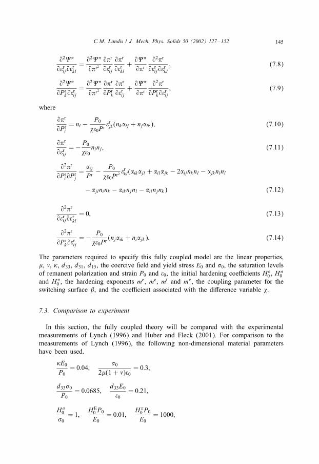
The parameters required to specify this fully coupled model are the linear properties,', (, �, d33, d31, d15, the coercive 4eld and yield stress E0 and �0, the saturation levelsof remanent polarization and strain P0 and �0, the initial hardening coeNcients H e

0 , H�0

and H20 , the hardening exponents me, mc, mt and m2, the coupling parameter for the

switching surface �, and the coeNcient associated with the diOerence variable 3.

7.3. Comparison to experiment

In this section, the fully coupled theory will be compared with the experimentalmeasurements of Lynch (1996) and Huber and Fleck (2001). For comparison to themeasurements of Lynch (1996), the following non-dimensional material parametershave been used.

�E0

P0= 0:04;

�0

2'(1 + ()�0= 0:3;

d33�0

P0= 0:0685;

d33E0

�0= 0:21;

H�0

�0= 1;

HE0 P0

E0= 0:01;

H20 P0

E0= 1000;


me = 2; mt = 2:75; mc = 1:5; m2 = 10;

( = 0:25; � = 2:75; 3 = 2:

Note that the piezoelectric coeNcients d31 and d15 are not required to model the uniax-ial electric 4eld—compressive stress experiments of Lynch (1996) or the experimentsof Huber and Fleck (2001) where there is no applied stress. Also note that Eq. (5.5)is not valid for �P since me = 2 has been used, instead �P is a logarithmic functionof Pr .

Figs. 3a–e plot the predicted constitutive behavior of a model ferroelectric with theparameters listed above. Again these parameters have been chosen to mimic the be-havior of the PLZT material that Lynch (1996) used to perform measurements on.Fig. 3a is a plot of the electric displacement versus electric 4eld hysteresis loop, andFig. 3b is the strain versus electric 4eld butter3y hysteresis loop. Fig. 3c is the strainversus electric displacement hysteresis loop that corresponds to the hysteresis and but-ter3y loops from Figs. 3a and b. Figs. 3d and e are the depolarization and stress–straincurves for an initially poled material. To obtain these curves, the material was initiallypoled with an electric 4eld of strength 3E0 and then the electric 4eld was removed.Thereafter, a compressive stress aligned with the polarization direction was appliedto the sample. Figs. 3d and e are the stress versus electric displacement and stressversus strain behavior of the ferroelectric during the application of the compressivestress. Each of these 4gures bears a qualitative, if not quantitative, resemblance to themeasured behavior on PLZT.

The hysteresis and butter3y loops that occur under the application of a constantapplied compressive stress are signi4cant features of ferroelectric constitutive behaviorthat were measured by Lynch (1996). Initially, the material is poled by a strong electric4eld and the 4eld is removed. Next, a compressive stress is applied and held constantat a given level. Finally, the electric 4eld is cycled and the resulting hysteresis andbutter3y loops are measured. The results from the fully coupled theory of Section 7that model these experiments are given in Fig. 4. Notice in Fig. 3e, the points labeledA, B and C. These points correspond to the hysteresis and butter3y loops labeledA, B and C in Fig. 4. Again, the agreement between the theory and experimentsis satisfactory. There is some evidence from the experiments that the wiggles in thehysteresis loops are physically realistic. However, the wiggles in the theoretical loopsare far more exaggerated than any wiggles seen in the experiments. It is possible thatthis feature could be corrected with modi4cations to the diOerence variable or thepotential associated with it.

Finally, the model is compared to the polarization rotation experiments of Huberand Fleck (2001). The experiments of Huber and Fleck (2001) are the only spatiallymulti-axial loading experiments on ferroelectric materials to date. During polarizationrotation experiments an electric 4eld is applied at some angle, /, to the initial polariza-tion direction. The polarization changes from its initial direction towards the directionof the applied electric 4eld. The physical quantities that are measured during the ex-periment are the applied electric 4eld and the change in electric displacement in thedirection of the applied electric 4eld. The predictions of the fully coupled theory withthe parameters used to model PLZT are shown as the bold lines in Fig. 5a. Predictions


Fig. 3. (a) D–E hysteresis loop, (b) �–E butter3y loop, (c) �–D hysteresis, (d) depolarization curve and(e) stress–strain curve derived from the fully coupled theory presented in Section 7.


Fig. 4. D–E hysteresis and �–E butter3y loops derived from the fully coupled theory of Section 7 whenthe material is subjected to a constant compressive stress. The loops labeled A, B and C correspond to thepoints A, B and C in Fig. 3e.


Fig. 5. (a) Predictions of the fully coupled theory of Section 7 and the uncoupled theory of Section 5for polarization rotation. (b) Comparison of the uncoupled theory of Section 5 to the polarization rotationexperiments of Huber and Fleck (2001).

from the uncoupled theory of Section 5 are shown as thin lines in Fig. 5a. Parame-ters for the uncoupled theory were chosen such that the hysteresis loops from the twocases were similar. Both the coupled and uncoupled theories are plotted in Fig. 5a todemonstrate that the predictions for the polarization rotation experiments are similar.This fact is important since a complete set of experiments like those done by Lynch(1996) was not available for the material used by Huber and Fleck (2001). Hence, theuncoupled theory is used to predict the polarization rotation experiments of Huber andFleck (2001) in Fig. 5b. The 4tting parameters listed in Fig. 5b are used to 4t the/ = 0◦ and / = 180◦ experimental data points. The agreement between the theory andthe remaining experiments appears to be satisfactory.

8. Discussion

The constitutive laws presented in this paper are internal variable theories. The inter-nal variables that de4ne the state of the material are the remanent polarization vectorand the second-order tensor of remanent strain. It is assumed that the internal stateof the material is uniquely de4ned by these variables. Associated with the internalvariables is a Helmholtz free energy potential from which hardening moduli are de-rived. The tensorial nature, i.e. the directional dependence, of the hardening moduli isreadily obtained from the invariants of the internal state variables. The dependence ofthe free energy on the invariants of the internal variables are then determined fromthe physics of the deformation and polarization processes in the material. For example,the free energy associated with the internal state variables increases dramatically as thepolarization or strain saturation conditions are approached.


A signi4cant feature of the constitutive laws derived in this paper is that they aresymmetric. In other words, a Maxwell relation holds for the tensors relating incre-ments of strain and electric displacement to increments of stress and electric 4eld.Speci4cally, the tangent piezoelectric tensor relating increments of strain to incrementsof electric 4eld is identical to the tangent piezoelectric tensor relating increments ofelectric displacement to increments of stress. Consequently, there exists a rate poten-tial from which stress and electric 4eld increments can be derived from strain andelectric displacement increments. This feature is possible due to the fact that the con-tribution to the dissipation rate from changes in material properties during switchingis accounted for. Accordingly, the material property changes must be and are includedin the switching surfaces and the 3ow rules. Constitutive laws that do not includematerial property changes within this type of consistent thermodynamic framework aregenerally not symmetric.

The symmetry of the tangent moduli is of notable importance in the development of4nite element equations used to solve complex boundary value problems. If the tangentmoduli are not symmetric then the 4nite element tangent stiOness matrix derived fromthem is not symmetric either. This is not to say that theories that do not producesymmetric tangent moduli are incorrect. However, computational storage requirementsand matrix inversion times are about a factor of two greater than the correspondingspace and time requirements for symmetric matrices.

Finally, and most importantly, the fully coupled constitutive law presented in Section7 has been shown to be in reasonable agreement with a wide range of experimental ob-servations on ferroelectric ceramics. Future experiments that may elucidate the shape ofthe switching surface or the functional form of the free energy potential will be helpfulin re4ning the features of the constitutive law. It is possible that other invariants thatcombine the strain and polarization, i.e. diOerence variables, may be more successfulthan 2r at describing a broader range of observations. This should not be interpretedas a de4ciency of the theory. On the contrary, the fact that alternative descriptionscan be used is a strength of the theory. There exists a degree of 3exibility within thethermodynamically consistent framework that can be used to re4ne and improve thedetails of the constitutive law.

Acknowledgements

I would like to thank Dr. John Huber for supplying the experimental data used inFig. 5b. I would also like to thank Professor Robert McMeeking for the manydiscussions that helped to shape this work.

Appendix: rate dependence

Rate dependence of the deformation and polarization response of ferroelectrics isconsidered in this appendix for two reasons. First, a rate-dependent constitutive lawin some cases more appropriately describes the physical behavior of ferroelectrics.


Second, it is simpler to numerically implement rate-dependent constitutive laws thantheir rate-independent counterparts. Fortunately, rate dependence 4ts directly into thethermodynamic framework already described. In the main body of this work, a su-perposed dot represents an in4nitesimal increment of the given quantity. However, inthis appendix, the superposed dot will now represent the time rate of change of thequantity.

The assumption that the remanent strain and remanent polarization characterize theinternal state of the material still holds for this excursion into rate dependence. Hence,Eqs. (3.1)–(3.13) remain valid. However, in place of Eqs. (3.14)–(3.16), the remanentstrain and polarization rates are now derived from a 3ow potential "(�ij ; Ei; �r

ij ; Pri ).

�rij =

9"9�ij

; (A.1)

Pri =

9"9Ei

: (A.2)

Unlike the " de4ned in the main body that had no restrictions on its dimensionality,the " used in Eqs. (A.1) and (A.2) must have dimensions of energy density rate.Then the strain and electric displacement rates remain as Eqs. (3.34) and (3.35), andthe constitutive law is complete. The consistency condition and the determination ofthe plastic multiplier are no longer required to complete the constitutive law. TheA-tensors are still de4ned by Eqs. (3.21)–(3.24), and the back stress, back electric4eld and hardening tensors are de4ned by Eqs. (3.9), (3.10) and (3.25)–(3.27). Notethat the 4nite element formulation required to implement the rate-dependent case willdiOer from Eq. (2.11).

Eqs. (3.34) and (3.35) may be written in another form. In a fashion similar to otherworks, e.g. Rice (1971), the strain and electric displacement rates can be split into“elastic” and “inelastic” parts, such that

�ij = �eij + �i

ij = sEijkl�kl + dkijEk + �i

ij ; (A.3)

Di = Dei + D

ii = dikl�kl + ��

ijEj + Dii ; (A.4)

where the inelastic strain rate, �iij, and inelastic electric displacement rate, D

ii can be

shown to be

�iij = �r

ij + A��ijkl�

rkl + A�P

kijPrk =

9"9�ij

; (A.5)

Dii = P

ri + AP�

ikl�rkl + APP

ij Prj =

9"9Ei

: (A.6)

Hence, the inelastic strain and electric displacement rates are normal to the 3owpotential in standard stress and electric 4eld space. This feature also holds for therate-independent case.


A simple example of the 3ow potential would be for a power law “visco-remanent”material where " is de4ned as

" = "0

(EiEi

E20

+3sij sij2�2

0+

�EiPrj sij

E0P0�0

)m

(A.7)

with this description of the 3ow potential, the rate-dependent case described here isidentical to the rate-independent form of Section 7 as the rate exponent, m → ∞.

References

Bassiouny, E., Ghaleb, A.F., Maugin, G.A., 1988a. Thermodynamical formulation for coupledelectromechanical hysteresis eOects—I. Basic equations. Int. J. Eng. Sci. 26, 1279–1295.

Bassiouny, E., Ghaleb, A.F., Maugin, G.A., 1988b. Thermodynamical formulation for coupledelectromechanical hysteresis eOects—II. Poling of ceramics. Int. J. Eng. Sci. 26, 1297–1306.

Bassiouny, E., Maugin, G.A., 1989a. Thermodynamical formulation for coupled electromechanical hysteresiseOects—III. Parameter identi4cation. Int. J. Eng. Sci. 27, 975–987.

Bassiouny, E., Maugin, G.A., 1989b. Thermodynamical formulation for coupled electromechanical hysteresiseOects—IV. Combined electromechanical loading. Int. J. Eng. Sci. 27, 989–1000.

Cocks, A.C.F., McMeeking, R.M., 1999. A phenomenological constitutive law for the behavior of ferroelectricceramics. Ferroelectrics 228, 219–228.

Drucker, D.C., 1952. A more fundamental approach to plastic stress–strain relations. Proceeding of the FirstU.S. Congress on Applied Mechanics, ASME, New York, pp. 487–491.

Fett, T., Muller, S., Munz, G., Thun, G., 1998. Nonsymmetry in the deformation behavior of PZT. J. Mat.Sci. Lett. 17, 261–265.

Huber, J.E., Fleck, N.A., 2001. Multi-axial electrical switching of a ferroelectric: theory versus experiment.J. Mech. Phys. Solids 49, 785–811.

Huber, J.E., Fleck, N.A., Landis, C.M., McMeeking, R.M., 1999. A constitutive model for ferroelectricpolycrystals. J. Mech. Phys. Solids 47, 1663–1697.

Kamlah, M., Tsakmakis, C., 1999. Phenomenological modeling of the non-linear electromechanical couplingin ferroelectrics. Int. J. Solids Struct. 36, 669–695.

Landis, C.M., 1999. Self-consistent and phenomenological constitutive models for ferroelectric ceramics.Ph.D. Thesis, University of California.

Landis, C.M., McMeeking, R.M., 1999. A phenomenological constitutive law for ferroelastic switching anda resulting asymptotic crack tip solution. J. Intelligent Mater. Systems Struct. 10, 155–163.

Lynch, C.S., 1996. The eOect of uniaxial stress on the electro-mechanical response of 8=65=35 PLZT. ActaMaterialia 44, 4137–4148.

McMeeking, R.M., 2000. Phenomenological constitutive models for ferroelectric ceramics. Presentation tothe SPIE, Newport Beach, CA.

Rice, J.R., 1971. Inelastic constitutive relations for solids: an internal-variable theory and its application tometal plasticity. J. Mech. Phys. Solids 19, 433–455.

Schneider, G.A., Heyer, V., 1999. In3uence of the electric 4eld on Vickers indentation crack growth inBaTiO3. J. European Ceramic Soc. 19, 1299–1306.

Fully coupled, multi-axial, symmetric constitutive laws ...

Documents

Transcript of Fully coupled, multi-axial, symmetric constitutive laws ...