Sensors 2013, 13, 3776-3798; doi:10.3390/s130303776

sensors ISSN 1424-8220

www.mdpi.com/journal/sensors

Article

Identifying Rhodamine Dye Plume Sources in Near-Shore

Oceanic Environments by Integration of Chemical and

Visual Sensors

Yu Tian 1, Xiaodong Kang

1, Yunyi Li

2, Wei Li

1,2,*, Aiqun Zhang

1, Jiangchen Yu

1 and

Yiping Li 1

1 State Key Laboratory of Robotics, Shenyang Institute of Automation, Chinese Academy of Sciences,

Shenyang 110016, China; E-Mails: tiany@sia.cn (Y.T.); kangxdcsu@163.com (X.K.);

zaq@sia.cn (A.Z.); yjc@sia.cn (J.Y.); lyp@sia.cn (Y.L.) 2

Department of Computer & Electrical Engineering and Computer Science,

California State University, Bakersfield, CA 93311, USA; E-Mail: yl180@duke.edu

* Author to whom correspondence should be addressed; E-Mail: wli@csub.edu;

Tel.: +1-661-654-6747; Fax: +1-661-654-6960.

Received: 3 February 2013; in revised form: 24 February 2013 / Accepted: 11 March 2013 /

Published: 18 March 2013

Abstract: This article presents a strategy for identifying the source location of a chemical

plume in near-shore oceanic environments where the plume is developed under the

influence of turbulence, tides and waves. This strategy includes two modules: source

declaration (or identification) and source verification embedded in a subsumption

architecture. Algorithms for source identification are derived from the moth-inspired plume

tracing strategies based on a chemical sensor. The in-water test missions, conducted in

November 2002 at San Clemente Island (California, USA) in June 2003 in Duck (North

Carolina, USA) and in October 2010 at Dalian Bay (China), successfully identified the

source locations after autonomous underwater vehicles tracked the rhodamine dye plumes

with a significant meander over 100 meters. The objective of the verification module is to

verify the declared plume source using a visual sensor. Because images taken in near shore

oceanic environments are very vague and colors in the images are not well-defined, we

adopt a fuzzy color extractor to segment the color components and recognize the chemical

plume and its source by measuring color similarity. The source verification module is

tested by images taken during the CPT missions.

OPEN ACCESS

Sensors 2013, 13 3777

Keywords: insect-inspired robots; chemical plume tracing; autonomous underwater vehicle;

odor source identification; fuzzy color segmentation

1. Introduction

Autonomous underwater vehicles (AUVs) with chemical plume tracing (CPT) capabilities would be

valuable in searching for deep sea hydrothermal vents, finding unexploded ordnance in near-shore oceanic

environments, and monitoring pollutants or localizing sources of hazardous chemicals in a harbor.

Factors that complicate CPT in natural environments (near-shore ocean conditions) include significant

filament intermittency and chemical plume meander, and flow variations with both location and time.

Over the last decade there has been interest in developing bio-inspired strategies for CPT in natural

environments. Belanger and Willis presented plume tracing strategies, including counter-turning strategies,

intended to mimic moth behavior and analyzed the performance in a computer simulation [1]. Li et al.

evaluated and optimized the moth-inspired plume tracing strategies using a simulated plume with

significant meander and intermittency of plume puffs [2]. Grasso and Basil presented biomimetic

strategies, inspired by lobsters, crayfishes, and crab, and used a lobster-inspired robot for locating an

odor source [3]. Minagawa et al. presented a crayfish robot employing flow induced by waving to

locate a chemical source [4]. Lochmatter and Martinoli tested the bio-inspired algorithms for tracking

odor plumes in a laminar wind field [5]. Swarm-based CPT algorithms inspired by insects, such as a

group of moths or an ant colony, are discussed in [6–8]. Most engineering-oriented algorithms for CPT

are comprehensively reviewed in [9].

Most of the existing studies have mainly focused on the plume tracing issue and validated their

algorithms in a small operation area in a range of centimeters to a few meters or in a simulated

environment, but they lacked detailed reports of CPT experiments in natural environments on a large

scale. The tracking of a chemical plume in the natural environment, such as near-shore oceanic

conditions, where the plume is developed under the influence of turbulence, tides and waves,

challenges CPT algorithms on how to cope with the intermittency of filaments and significant plume

meander. The lack of correlation between the fluid flow direction and the plume long axis often causes

an AUV to lose contact with the plume because the instantaneous fluid flow direction within a plume

with significant meander is not always aligned with the plume’s long axis [10]. Conducting CPT

missions in near-shore ocean environments on a large scale has to consider the full spectrum of field

behavior that include plume finding, plume following, maneuvers to recontact a lost plume, and

declaration that the source has been found [2]. Li et al. proposed a subsumption architecture for CPT

missions [11], consisting of these four fundamental behaviors: finding the plume, maintaining the

plume, reacquiring the plume, and declaring the source location or identifying the source location.

Our research mainly focuses on the plume source identification issue in real world scenarios. The

strategy discussed herein includes two modules: Source declaration (or identification) and source

verification. This article presents the experimental results on identifying rhodamine dye plume sources

in near-shore oceanic environments to validate two variations of the source identification algorithms

SIZ_T and SIZ_F described in [12]. For the in-water tests, the SIZ_T algorithm was implemented on a

Sensors 2013, 13 3778

REMUS vehicle, developed by the Oceanographic Systems Laboratory at the Woods Hole

Oceanographic Institute [11,13], as shown in Figure 1. In order to validate the SIZ_F algorithm [14],

Shenyang Institute of Automation (SIA), Chinese Academy of Sciences, developed a new AUV plume

tracer and an alternative strategy for generating a rhodamine dye plume in near-ocean environment.

Figure 2 shows the mission MSN171639 conducted at Dalai Bay (China) in October 2010.

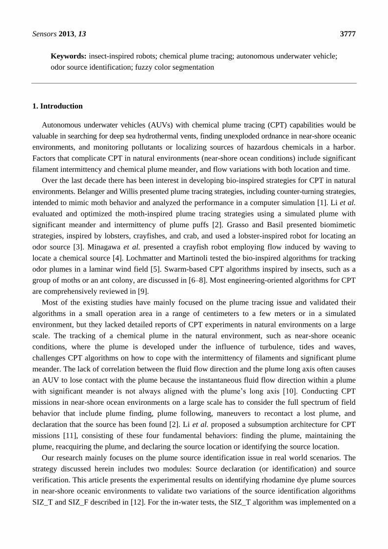
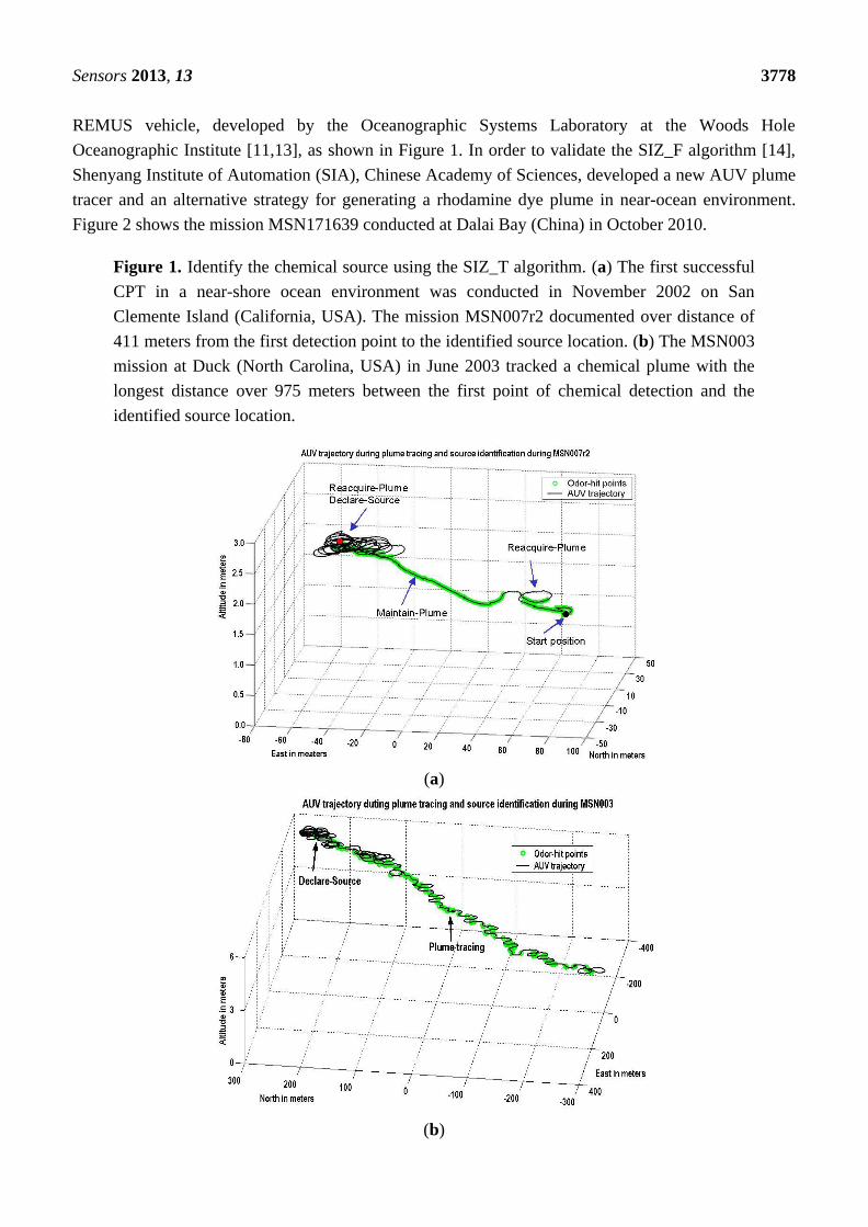
Figure 1. Identify the chemical source using the SIZ_T algorithm. (a) The first successful

CPT in a near-shore ocean environment was conducted in November 2002 on San

Clemente Island (California, USA). The mission MSN007r2 documented over distance of

411 meters from the first detection point to the identified source location. (b) The MSN003

mission at Duck (North Carolina, USA) in June 2003 tracked a chemical plume with the

longest distance over 975 meters between the first point of chemical detection and the

identified source location.

(a)

(b)

Sensors 2013, 13 3779

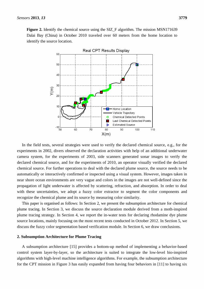
Figure 2. Identify the chemical source using the SIZ_F algorithm. The mission MSN171639

Dalai Bay (China) in October 2010 traveled over 60 meters from the home location to

identify the source location.

In the field tests, several strategies were used to verify the declared chemical source, e.g., for the

experiments in 2002, divers observed the declaration activities with help of an additional underwater

camera system, for the experiments of 2003, side scanners generated sonar images to verify the

declared chemical source, and for the experiments of 2010, an operator visually verified the declared

chemical source. For further operations to deal with the declared plume source, the source needs to be

automatically or interactively confirmed or inspected using a visual system. However, images taken in

near shore ocean environments are very vague and colors in the images are not well-defined since the

propagation of light underwater is affected by scattering, refraction, and absorption. In order to deal

with these uncertainties, we adopt a fuzzy color extractor to segment the color components and

recognize the chemical plume and its source by measuring color similarity.

This paper is organised as follows: In Section 2, we present the subsumption architecture for chemical

plume tracing. In Section 3, we discuss the source declaration module derived from a moth-inspired

plume tracing strategy. In Section 4, we report the in-water tests for declaring rhodamine dye plume

source locations, mainly focusing on the most recent tests conducted in October 2012. In Section 5, we

discuss the fuzzy color segmentation based verification module. In Section 6, we draw conclusions.

2. Subsumption Architecture for Plume Tracing

A subsumption architecture [15] provides a bottom-up method of implementing a behavior-based

control system layer-by-layer, so the architecture is suited to integrate the low-level bio-inspired

algorithms with high-level machine intelligence algorithms. For example, the subsumption architecture

for the CPT mission in Figure 3 has easily expanded from having four behaviors in [11] to having six

Sensors 2013, 13 3780

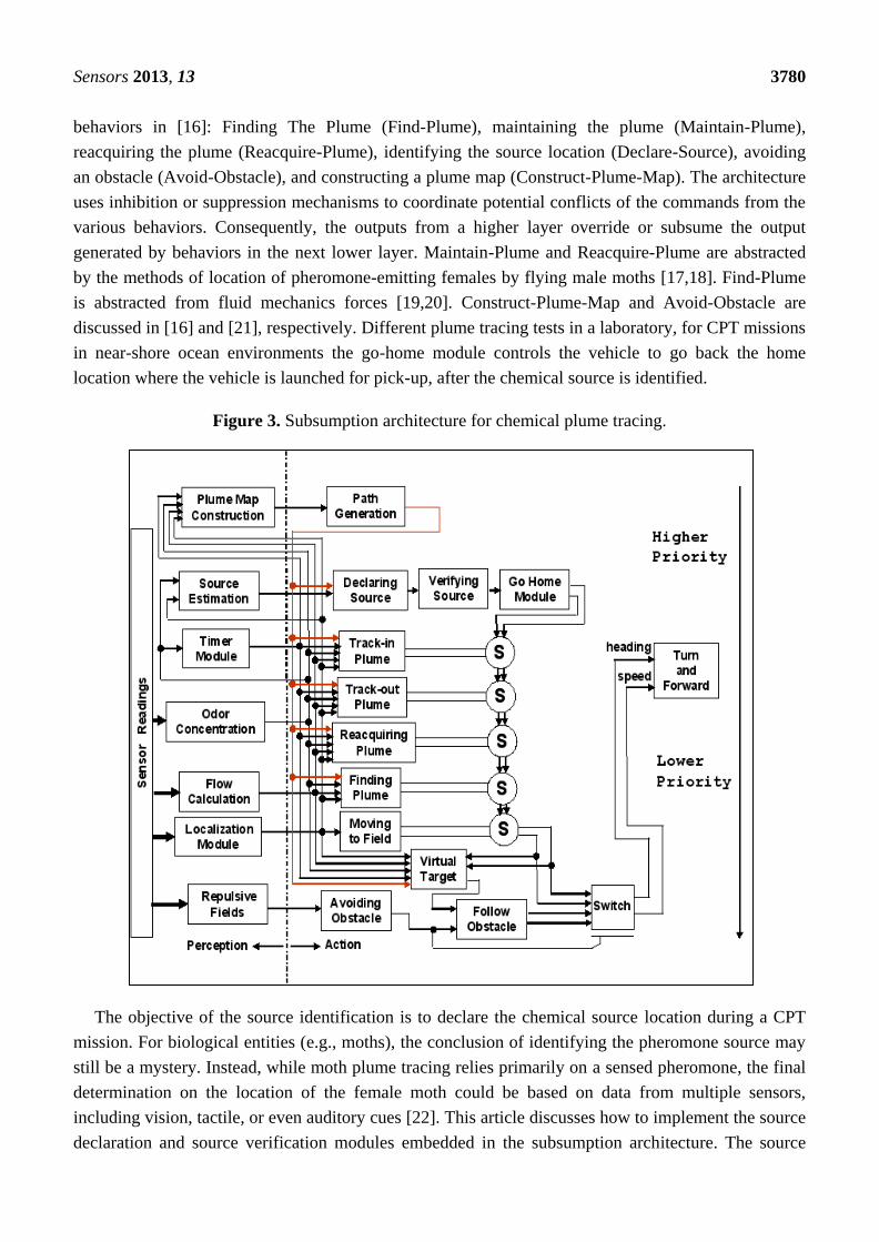
behaviors in [16]: Finding The Plume (Find-Plume), maintaining the plume (Maintain-Plume),

reacquiring the plume (Reacquire-Plume), identifying the source location (Declare-Source), avoiding

an obstacle (Avoid-Obstacle), and constructing a plume map (Construct-Plume-Map). The architecture

uses inhibition or suppression mechanisms to coordinate potential conflicts of the commands from the

various behaviors. Consequently, the outputs from a higher layer override or subsume the output

generated by behaviors in the next lower layer. Maintain-Plume and Reacquire-Plume are abstracted

by the methods of location of pheromone-emitting females by flying male moths [17,18]. Find-Plume

is abstracted from fluid mechanics forces [19,20]. Construct-Plume-Map and Avoid-Obstacle are

discussed in [16] and [21], respectively. Different plume tracing tests in a laboratory, for CPT missions

in near-shore ocean environments the go-home module controls the vehicle to go back the home

location where the vehicle is launched for pick-up, after the chemical source is identified.

Figure 3. Subsumption architecture for chemical plume tracing.

The objective of the source identification is to declare the chemical source location during a CPT

mission. For biological entities (e.g., moths), the conclusion of identifying the pheromone source may

still be a mystery. Instead, while moth plume tracing relies primarily on a sensed pheromone, the final

determination on the location of the female moth could be based on data from multiple sensors,

including vision, tactile, or even auditory cues [22]. This article discusses how to implement the source

declaration and source verification modules embedded in the subsumption architecture. The source

Sensors 2013, 13 3781

declaration module uses plume events detected by a chemical sensor, in combination with measured

AUV locations and fluid flow directions, to identify the plume source location, while the source

verification module uses fuzzy color segmentation algorithms to recognize the chemical plume and its

source in an image taken when the source is declared.

3. Source Declaration Module

This section briefly presents the source identification algorithms derived from the two

moth-inspired behaviors: Maintain-Plume and Reacquire-Plume. Maintain-Plume is broken down into

Track-In and Track-Out activities due to intermittency of a chemical plume transported in a fluid flow

environment [12]. An AUV alternatively utilizes Maintain-Plume and Reacquire-Plume in making

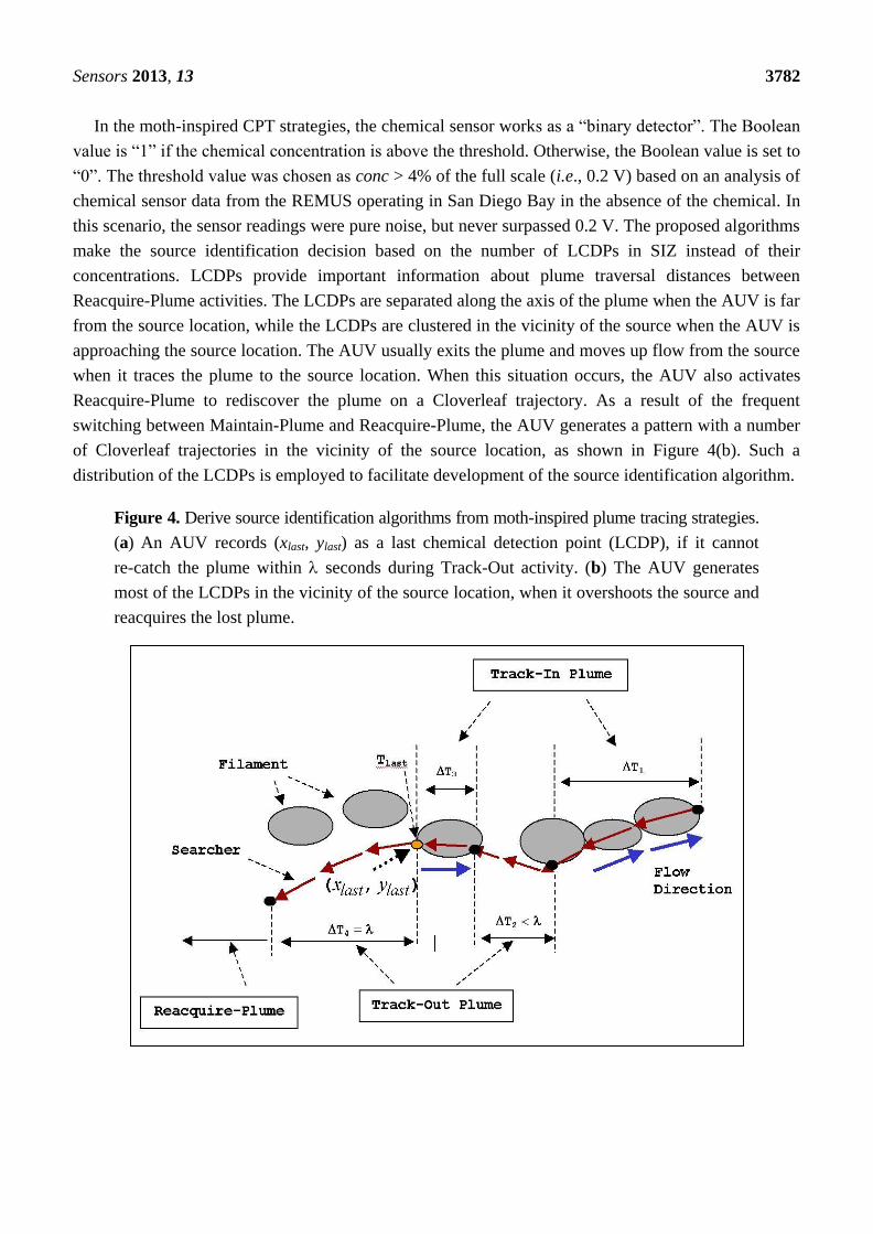
progress towards the source location in the up-flow direction. In a typical scenario of plume tracing,

the AUV activates Track-In once it detects the chemical, e.g., the activities during and in

Figure 4(a). It continues Track-Out when it loses contact with the chemical within λ seconds, e.g., the

activity during in Figure 4(a). After λ seconds, it switches to Reacquire-Plume for casting the

plume, e.g., the activity after in Figure 4(a).

A chemical detection point at which the AUV loses contact with the chemical plume for λ seconds

is defined as a LCDP, e.g., point (xlast, ylast) at in Figure 4(a). In our applications, the coordinates

of (xlast, ylast) are specified in a coordinate system with the origin defined by the center of an operation

area. We use a Cloverleaf trajectory with the center (xlast, ylast) to implement the Reacquire-Plume

behavior, as shown in Figure 4(b). Note that one leaf is aligned with the down-flow direction for the

AUV to rediscover the chemical when it has passed the source location. During a Reacquire-Plume

activity, the AUV either detects the chemical or completes the Cloverleaf trajectory Nre times

(Nre = 2 or 3 for the in-waters). The length of each leaf of the Cloverleaf trajectory is constrained to be

larger than the AUV turning radius about 15 meters. If Nre repetitions are completed without a

chemical detection, the AUV reverts to Find-Plume. Here, we define a LCDP node by:

struct LCDP_Node

{

double , , ;

double conc, , ;

double ,

};

where Tlast is the time when the LCDP is detected, (xlast, ylast) are the coordinates of the AUV at Tlast,

conc is the chemical concentration at (xlast, ylast) and Tlast, (fdir,fmag) are the flow direction and

magnitude at (xlast, ylast) and Tlast, and (xflow, yflow) are the coordinates in a new coordinate system

defined according to the current flow direction. For convenience, we also use (xlast, ylast) to represent

the LCDP in the following discussion.

lastT

lastT lastx lasty

dirf magf

flowx flowy

Sensors 2013, 13 3782

In the moth-inspired CPT strategies, the chemical sensor works as a “binary detector”. The Boolean

value is “1” if the chemical concentration is above the threshold. Otherwise, the Boolean value is set to

“0”. The threshold value was chosen as conc > 4% of the full scale (i.e., 0.2 V) based on an analysis of

chemical sensor data from the REMUS operating in San Diego Bay in the absence of the chemical. In

this scenario, the sensor readings were pure noise, but never surpassed 0.2 V. The proposed algorithms

make the source identification decision based on the number of LCDPs in SIZ instead of their

concentrations. LCDPs provide important information about plume traversal distances between

Reacquire-Plume activities. The LCDPs are separated along the axis of the plume when the AUV is far

from the source location, while the LCDPs are clustered in the vicinity of the source when the AUV is

approaching the source location. The AUV usually exits the plume and moves up flow from the source

when it traces the plume to the source location. When this situation occurs, the AUV also activates

Reacquire-Plume to rediscover the plume on a Cloverleaf trajectory. As a result of the frequent

switching between Maintain-Plume and Reacquire-Plume, the AUV generates a pattern with a number

of Cloverleaf trajectories in the vicinity of the source location, as shown in Figure 4(b). Such a

distribution of the LCDPs is employed to facilitate development of the source identification algorithm.

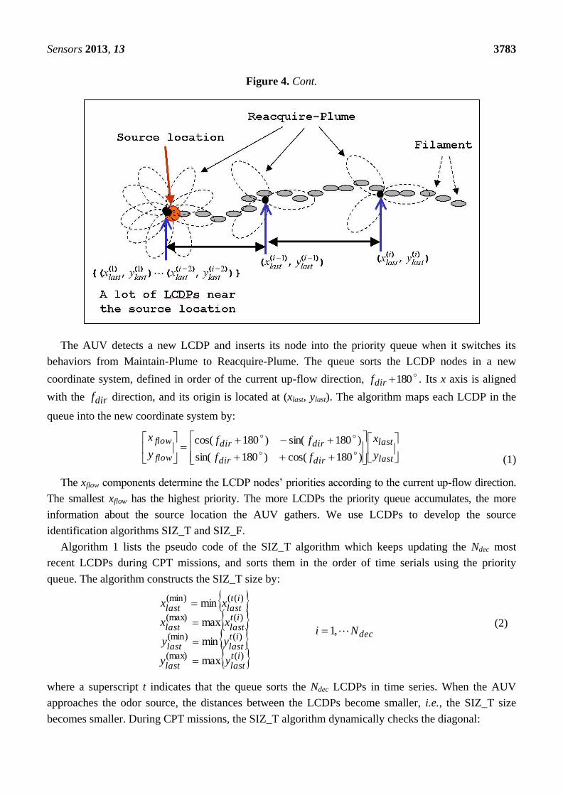
Figure 4. Derive source identification algorithms from moth-inspired plume tracing strategies.

(a) An AUV records (xlast, ylast) as a last chemical detection point (LCDP), if it cannot

re-catch the plume within seconds during Track-Out activity. (b) The AUV generates

most of the LCDPs in the vicinity of the source location, when it overshoots the source and

reacquires the lost plume.

Sensors 2013, 13 3783

Figure 4. Cont.

The AUV detects a new LCDP and inserts its node into the priority queue when it switches its

behaviors from Maintain-Plume to Reacquire-Plume. The queue sorts the LCDP nodes in a new

coordinate system, defined in order of the current up-flow direction, 180dirf . Its x axis is aligned

with the dirf direction, and its origin is located at (xlast, ylast). The algorithm maps each LCDP in the

queue into the new coordinate system by:

(1)

The xflow components determine the LCDP nodes’ priorities according to the current up-flow direction.

The smallest xflow has the highest priority. The more LCDPs the priority queue accumulates, the more

information about the source location the AUV gathers. We use LCDPs to develop the source

identification algorithms SIZ_T and SIZ_F.

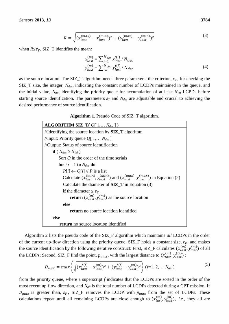
Algorithm 1 lists the pseudo code of the SIZ_T algorithm which keeps updating the Ndec most

recent LCDPs during CPT missions, and sorts them in the order of time serials using the priority

queue. The algorithm constructs the SIZ_T size by:

(2)

where a superscript t indicates that the queue sorts the Ndec LCDPs in time series. When the AUV

approaches the odor source, the distances between the LCDPs become smaller, i.e., the SIZ_T size

becomes smaller. During CPT missions, the SIZ_T algorithm dynamically checks the diagonal:

last

last

dirdir

dirdir

flow

flow

y

x

ff

ff

y

x

)180cos()180sin(

)180sin()180cos(

dec

itlastlast

itlastlast

itlastlast

itlastlast

Ni

yy

yy

xx

xx

,1

max

min

max

min

)((max)

)((min)

)((max)

)(((min)

Sensors 2013, 13 3784

(3)

when R , SIZ_T identifies the mean:

(4)

as the source location. The SIZ_T algorithm needs three parameters: the criterion, , for checking the

SIZ_T size, the integer, Ndec, indicating the constant number of LCDPs maintained in the queue, and

the initial value, Nini, identifying the priority queue for accumulation of at least Nini LCPDs before

starting source identification. The parameters and Ndec are adjustable and crucial to achieving the

desired performance of source identification.

Algorithm 1. Pseudo Code of SIZ_T algorithm.

ALGORITHM SIZ_T( Q[ 1,… Ndec ] )

//Identifying the source location by SIZ_T algorithm

//Input: Priority queue Q[ 1,… Ndec ]

//Output: Status of source identification

if ( Ndec Nini )

Sort Q in the order of the time serials

for i 1 to Ndec do

P[i] Q[i] // P is a list

Calculate

and

in Equation (2)

Calculate the diameter of SIZ_T in Equation (3)

if the diameter

return

as the source location

else

return no source location identified

else

return no source location identified

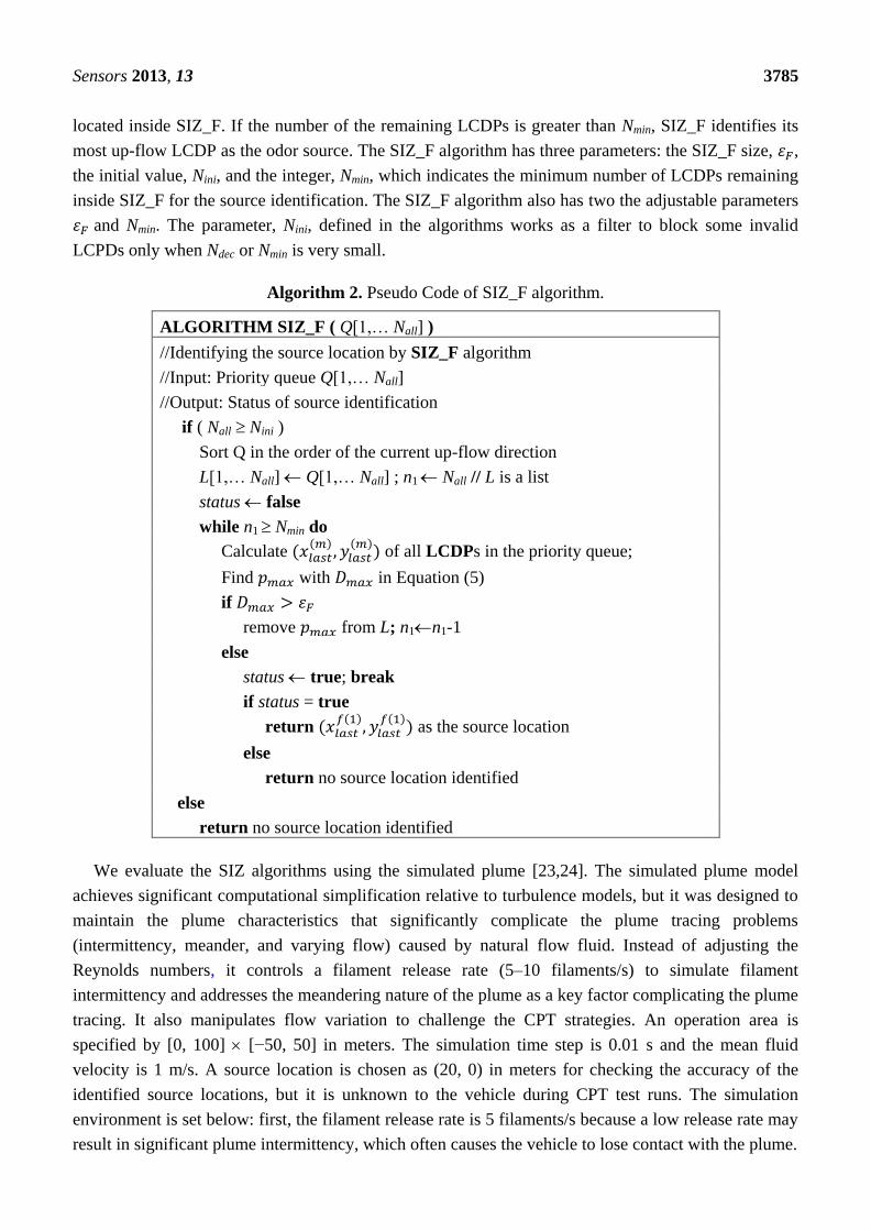
Algorithm 2 lists the pseudo code of the SIZ_F algorithm which maintains all LCDPs in the order

of the current up-flow direction using the priority queue. SIZ_F holds a constant size, , and makes

the source identification by the following iterative construct: First, SIZ_F calculates

of all

the LCDPs; Second, SIZ_F find the point, , with the largest distance to

:

1, 2, (5)

from the priority queue, where a superscript f indicates that the LCDPs are sorted in the order of the

most recent up-flow direction, and Nall is the total number of LCDPs detected during a CPT mission. If

is greater than, , SIZ_F removes the LCDP with from the set of LCDPs. These

calculations repeat until all remaining LCDPs are close enough to

, i.e., they all are

decN

i

itlast

mlast

decN

i

itlast

mlast

Nyy

Nxx

dec

dec

/

/

1

)()(1

)()(

Sensors 2013, 13 3785

located inside SIZ_F. If the number of the remaining LCDPs is greater than Nmin, SIZ_F identifies its

most up-flow LCDP as the odor source. The SIZ_F algorithm has three parameters: the SIZ_F size, ,

the initial value, Nini, and the integer, Nmin, which indicates the minimum number of LCDPs remaining

inside SIZ_F for the source identification. The SIZ_F algorithm also has two the adjustable parameters

and Nmin. The parameter, Nini, defined in the algorithms works as a filter to block some invalid

LCPDs only when Ndec or Nmin is very small.

Algorithm 2. Pseudo Code of SIZ_F algorithm.

ALGORITHM SIZ_F ( Q[1,… Nall] )

//Identifying the source location by SIZ_F algorithm

//Input: Priority queue Q[1,… Nall]

//Output: Status of source identification

if ( Nall Nini )

Sort Q in the order of the current up-flow direction

L[1,… Nall] Q[1,… Nall] ; n1 Nall // L is a list

status false

while n1 Nmin do

Calculate

of all LCDPs in the priority queue;

Find with in Equation (5)

if

remove from L; n1n1-1

else

status true; break

if status = true

return

as the source location

else

return no source location identified

else

return no source location identified

We evaluate the SIZ algorithms using the simulated plume [23,24]. The simulated plume model

achieves significant computational simplification relative to turbulence models, but it was designed to

maintain the plume characteristics that significantly complicate the plume tracing problems

(intermittency, meander, and varying flow) caused by natural flow fluid. Instead of adjusting the

Reynolds numbers, it controls a filament release rate (5–10 filaments/s) to simulate filament

intermittency and addresses the meandering nature of the plume as a key factor complicating the plume

tracing. It also manipulates flow variation to challenge the CPT strategies. An operation area is

specified by [0, 100] [−50, 50] in meters. The simulation time step is 0.01 s and the mean fluid

velocity is 1 m/s. A source location is chosen as (20, 0) in meters for checking the accuracy of the

identified source locations, but it is unknown to the vehicle during CPT test runs. The simulation

environment is set below: first, the filament release rate is 5 filaments/s because a low release rate may

result in significant plume intermittency, which often causes the vehicle to lose contact with the plume.

Sensors 2013, 13 3786

The SIZ_T condition is stronger than the SIZ_F condition as SIZ_T requires the AUV to generate a

few of the most recent LCDPs close enough in the vicinity of the odor source. However, it is not

always true because the AUV may exit both sides of plumes in the vicinity of the source location due

to the width of chemical plumes, the variation of flow directions, the intermittency of filaments, or the

vehicle’s mechanical restrains. For source declaration, SIZ_F needs a few of the most up-flow LCDPs

close enough so it is suggested to use SIZ_F to identify a static plume source since the odor source

located in the up-flow direction always makes the AUV progress up-flow.

4. In-Water Tests for Declaring Rhodamine Dye Plume Sources

A type of SIZ_T algorithms is implemented on the REMUS vehicle for the CPT missions. The

initial values of SIZ_T were chosen and Ndec = 3 prior to the 2002 CPT missions. Eight of the

first ten runs aborted due to vehicle issues, including start-up problems, incorrect time settings,

equipment failure, etc. The other two test runs performed plume tracing well, but source declaration

did not occur as both and Ndec were too small. We empirically changed to and Ndec = 6

(our Monte Carlo evaluations in [25] show this set of parameters has a success rate of 96.8%). These

settings successfully declared the source locations of rhodamine dye plumes, as shown in Figure 5, for

the last seven test runs at the San Clemente Island (California, USA) in November 2002 labeled as

MSN007r2–MSN010r3. Figure 1(a) shows the mission MSN007r2 that documented over a distance of

411 meters from the first detection point to the identified source location. In the in-water tests in April

2003 at San Clemente Island, the same settings successfully identified the source location on seven of

eight experiments. The experiments included ground truth confirmation of identified source locations

via sidescan sonar with 8–17 m accuracy. These settings were also successfully used for the in-water

tests conducted in June 2003 in Duck (North Carolina, USA) in an operation area of

367 × 1,094 m (bigger than 60 football fields). Two types of missions were of interest during this set

of experiments. The first mission type involved a single chemical source in the operation area. The

second mission type may contain a few chemical sources in the operation area. The two types of CPT

mission successfully identified the source locations with ground truth confirmation via sidescan sonar

with 6–31 m accuracy [13]. Figure 1(b) shows the MSN003 mission at Duck in June 2003. This

mission tracked the chemical plume for 976 m between the first detection point and the declared

source location, with 13 m accuracy.

The most recent in-water tests for identifying rhodamine dye plume sources were conducted in

October 2010 at Dalian Bay (China). For this set of field tests, we implemented the SIZ_F algorithm

on the AUV developed by SIA. The parameters and Nmin= 6 in SIZ_F are optimized in [12]

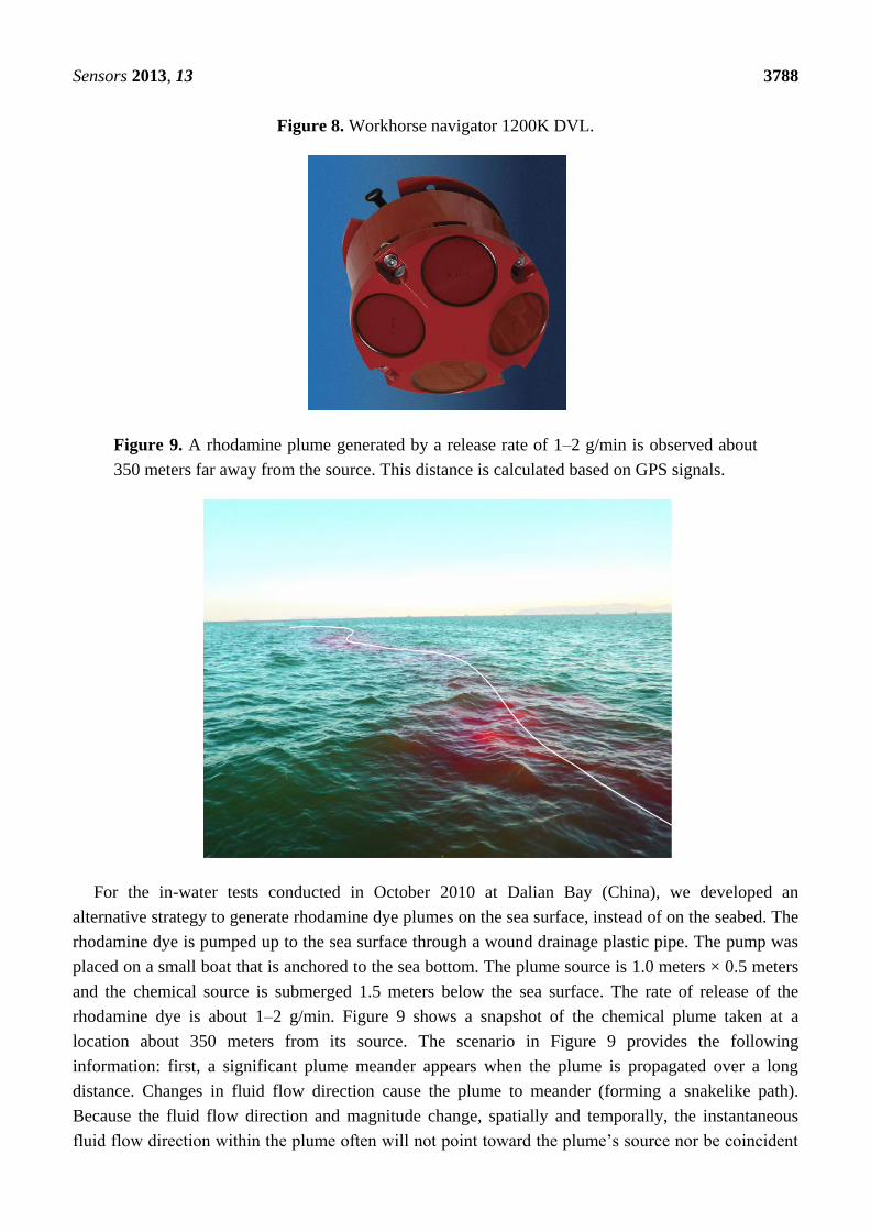
prior to the 2012 CPT missions. The AUV shown in Figure 6 is equipped with multiple sensors,

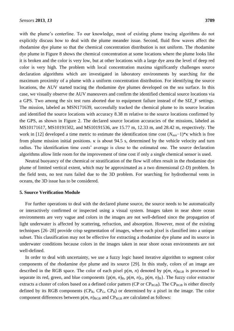
including a depth sensor, an underwater fluorometer, and a Doppler Velocity Log (DVL), etc. Figure 7

shows the fluorometer Cyclops-7 produced by Turner Designs, Inc. (Sunnyvale, CA, USA). Its

technical specifications can be found at http://www.turnerdesigns.com/products/ submersible/cyclops-

7. The AUV uses the fluorometer to detect rhodamine dye plume concentration. For the in-water tests,

we set the sampling rate of the fluorometer as 10 Hz and choose the 0–10 ug/L measurement scale in

which the fluorometer outputs 5 VDC corresponding to a rhodamine dye concentration of 10 μg/L.

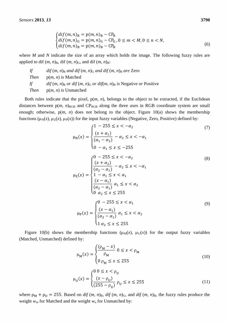
Figure 8 shows the workhorse navigator 1200K DVL produced by Teledyne RD Instruments (Poway,

Sensors 2013, 13 3787

CA, USA), and its technical specifications can be found at http://www.rdinstruments.com/pdfs/

wh_navigator_ds_lr.pdf. The DVL measures the AUV speed relative to the sea bottom based on which

we use the dead reckoning method to estimate AUV positions as well as fluid speed and orientation.

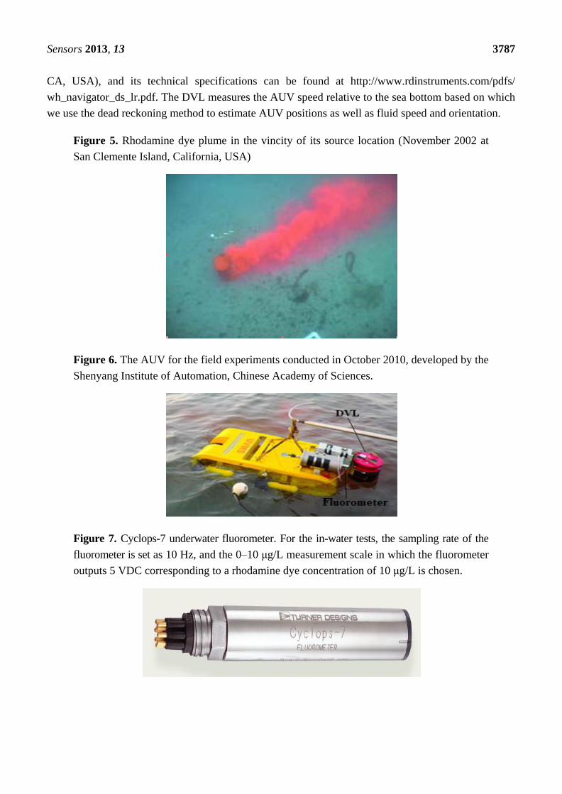
Figure 5. Rhodamine dye plume in the vincity of its source location (November 2002 at

San Clemente Island, California, USA)

Figure 6. The AUV for the field experiments conducted in October 2010, developed by the

Shenyang Institute of Automation, Chinese Academy of Sciences.

Figure 7. Cyclops-7 underwater fluorometer. For the in-water tests, the sampling rate of the

fluorometer is set as 10 Hz, and the 0–10 μg/L measurement scale in which the fluorometer

outputs 5 VDC corresponding to a rhodamine dye concentration of 10 μg/L is chosen.

Sensors 2013, 13 3788

Figure 8. Workhorse navigator 1200K DVL.

Figure 9. A rhodamine plume generated by a release rate of 1–2 g/min is observed about

350 meters far away from the source. This distance is calculated based on GPS signals.

For the in-water tests conducted in October 2010 at Dalian Bay (China), we developed an

alternative strategy to generate rhodamine dye plumes on the sea surface, instead of on the seabed. The

rhodamine dye is pumped up to the sea surface through a wound drainage plastic pipe. The pump was

placed on a small boat that is anchored to the sea bottom. The plume source is 1.0 meters × 0.5 meters

and the chemical source is submerged 1.5 meters below the sea surface. The rate of release of the

rhodamine dye is about 1–2 g/min. Figure 9 shows a snapshot of the chemical plume taken at a

location about 350 meters from its source. The scenario in Figure 9 provides the following

information: first, a significant plume meander appears when the plume is propagated over a long

distance. Changes in fluid flow direction cause the plume to meander (forming a snakelike path).

Because the fluid flow direction and magnitude change, spatially and temporally, the instantaneous

fluid flow direction within the plume often will not point toward the plume’s source nor be coincident

Sensors 2013, 13 3789

with the plume’s centerline. To our knowledge, most of existing plume tracing algorithms do not

explicitly discuss how to deal with the plume meander issue. Second, fluid flow waves affect the

rhodamine dye plume so that the chemical concentration distribution is not uniform. The rhodamine

dye plume in Figure 8 shows the chemical concentration at some locations where the plume looks like

it is broken and the color is very low, but at other locations with a large dye area the level of deep red

color is very high. The problem with local concentration maxima significantly challenges source

declaration algorithms which are investigated in laboratory environments by searching for the

maximum proximity of a plume with a uniform concentration distribution. For identifying the source

locations, the AUV started tracing the rhodamine dye plumes developed on the sea surface. In this

case, we visually observe the AUV maneuvers and confirm the identified chemical source locations via

a GPS. Two among the six test runs aborted due to equipment failure instead of the SIZ_F settings.

The mission, labeled as MSN171639, successfully tracked the chemical plume to its source location

and identified the source locations with accuracy 8.38 m relative to the source locations confirmed by

the GPS, as shown in Figure 2. The declared source location accuracies of the missions, labeled as

MS10171617, MS10191502, and MS10191536, are 15.77 m, 12.33 m, and 28.42 m, respectively. The

work in [12] developed a time metric to estimate the identification time cost (Nmin−1)*κ which is free

from plume mission initial positions. κ is about 94.5 s, determined by the vehicle velocity and turn

radius. The identification time costs’ average is close to the estimated one. The source declaration

algorithms allow little room for the improvement of time cost if only a single chemical sensor is used.

Neutral buoyancy of the chemical or stratification of the flow will often result in the rhodamine dye

plume of limited vertical extent, which may be approximated as a two dimensional (2-D) problem. In

the field tests, no test runs failed due to the 3D problem. For searching for hydrothermal vents in

oceans, the 3D issue has to be considered.

5. Source Verification Module

For further operations to deal with the declared plume source, the source needs to be automatically

or interactively confirmed or inspected using a visual system. Images taken in near shore ocean

environments are very vague and colors in the images are not well-defined since the propagation of

light underwater is affected by scattering, refraction, and absorption. However, most of the existing

techniques [26–28] provide crisp segmentation of images, where each pixel is classified into a unique

subset. This classification may not be effective for extracting a rhodamine dye plume and its source in

underwater conditions because colors in the images taken in near shore ocean environments are not

well-defined.

In order to deal with uncertainty, we use a fuzzy logic based iterative algorithm to segment color

components of the rhodamine dye plume and its source [29]. In this study, colors of an image are

described in the RGB space. The color of each pixel p(m, n) denoted by p(m, n)RGB is processed to

separate its red, green, and blue components {p(m, n)R, p(m, n)G, p(m, n)B}. The fuzzy color extractor

extracts a cluster of colors based on a defined color pattern (CP or CPRGB). The CPRGB is either directly

defined by its RGB components (CPR, CPG, CPB) or determined by a pixel in the image. The color

component differences between p(m, n)RGB and CPRGB are calculated as follows:

Sensors 2013, 13 3790

(6)

where M and N indicate the size of an array which holds the image. The following fuzzy rules are

applied to dif (m, n)R, dif (m, n)G, and dif (m, n)B:

If dif (m, n)R and dif (m, n)G and dif (m, n)B are Zero

Then p(m, n) is Matched

If dif (m, n)R or dif (m, n)G or dif(m, n)B is Negative or Positive

Then p(m, n) is Unmatched

Both rules indicate that the pixel, p(m, n), belongs to the object to be extracted, if the Euclidean

distances between p(m, n)RGB and CPRGB along the three axes in RGB coordinate system are small

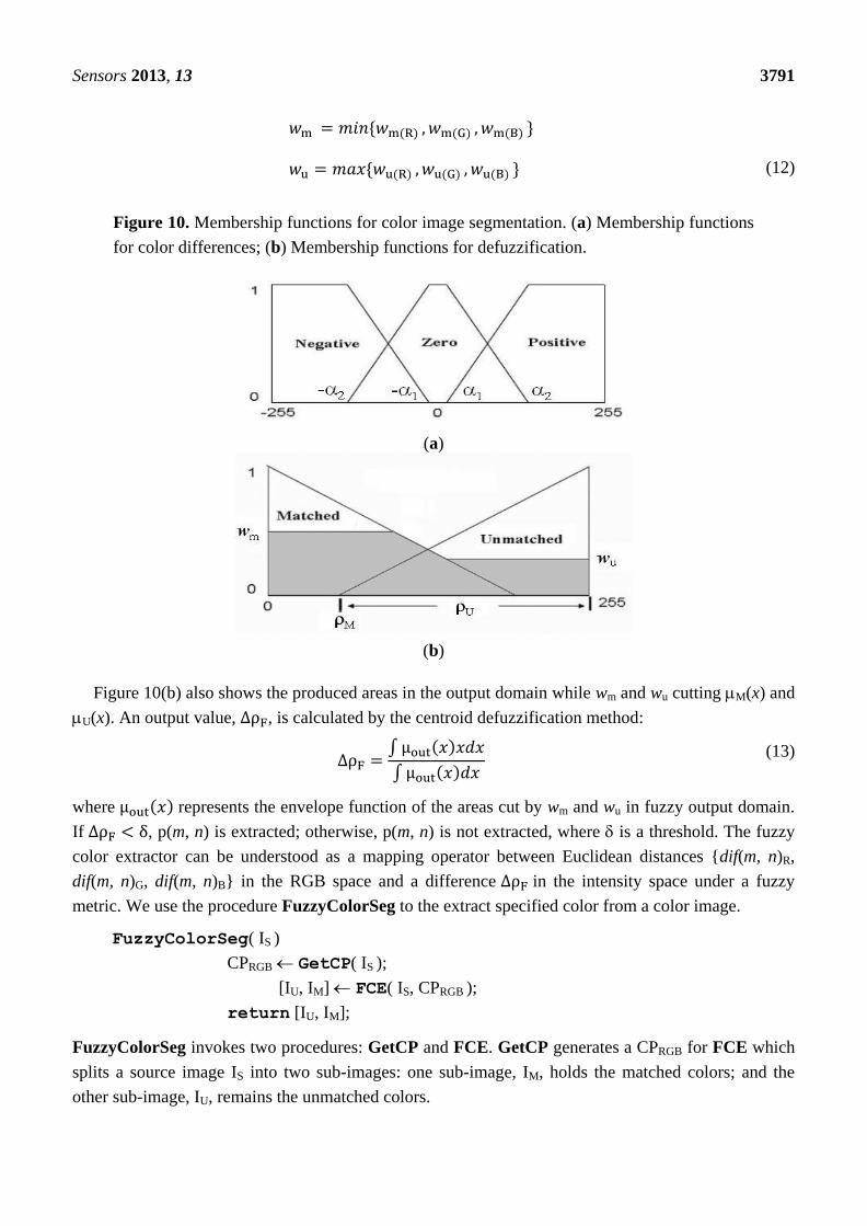
enough; otherwise, p(m, n) does not belong to the object. Figure 10(a) shows the membership

functions (N(x), Z(x), P(x)) for the input fuzzy variables (Negative, Zero, Positive) defined by:

(7)

(8)

(9)

Figure 10(b) shows the membership functions (M(x), U(x)) for the output fuzzy variables

(Matched, Unmatched) defined by:

μ

(10)

μ

(11)

where . Based on dif (m, n)R, dif (m, n)G, and dif (m, n)B, the fuzzy rules produce the

weight wm for Matched and the weight wu for Unmatched by:

Sensors 2013, 13 3791

(12)

Figure 10. Membership functions for color image segmentation. (a) Membership functions

for color differences; (b) Membership functions for defuzzification.

(a)

(b)

Figure 10(b) also shows the produced areas in the output domain while wm and wu cutting M(x) and

U(x). An output value, , is calculated by the centroid defuzzification method:

(13)

where represents the envelope function of the areas cut by wm and wu in fuzzy output domain.

If , p(m, n) is extracted; otherwise, p(m, n) is not extracted, where is a threshold. The fuzzy

color extractor can be understood as a mapping operator between Euclidean distances {dif(m, n)R,

dif(m, n)G, dif(m, n)B} in the RGB space and a difference in the intensity space under a fuzzy

metric. We use the procedure FuzzyColorSeg to the extract specified color from a color image.

FuzzyColorSeg( IS )

CPRGB GetCP( IS );

[IU, IM] FCE( IS, CPRGB );

return [IU, IM];

FuzzyColorSeg invokes two procedures: GetCP and FCE. GetCP generates a CPRGB for FCE which

splits a source image IS into two sub-images: one sub-image, IM, holds the matched colors; and the

other sub-image, IU, remains the unmatched colors.

Sensors 2013, 13 3792

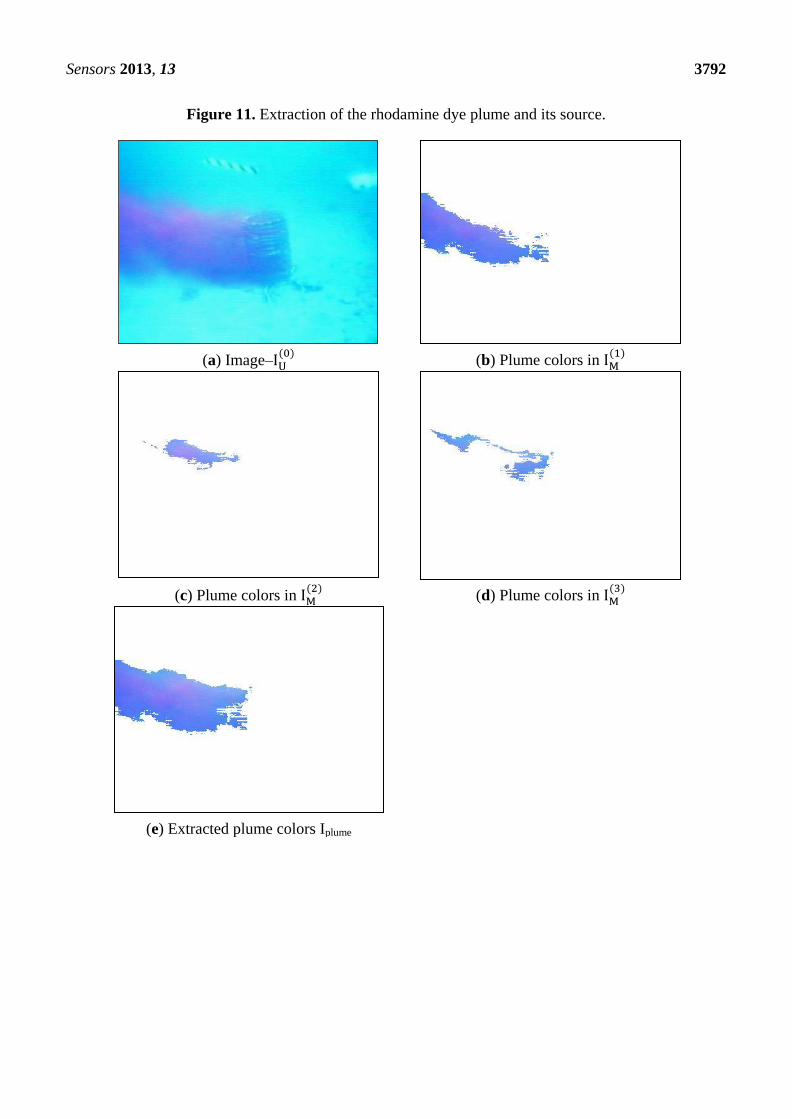
Figure 11. Extraction of the rhodamine dye plume and its source.

(a) Image–

(b) Plume colors in

(c) Plume colors in

(d) Plume colors in

(e) Extracted plume colors Iplume

Sensors 2013, 13 3793

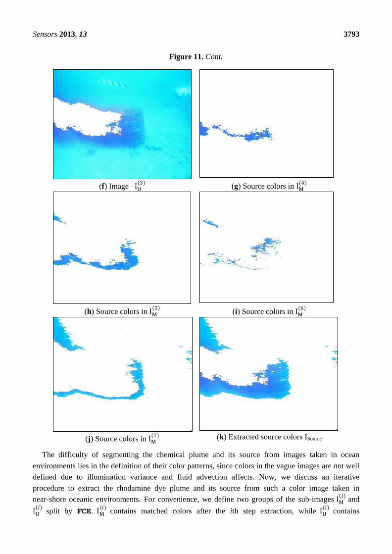
Figure 11. Cont.

(f) Image –

(g) Source colors in

(h) Source colors in

(i) Source colors in

(j) Source colors in

(k) Extracted source colors ISource

The difficulty of segmenting the chemical plume and its source from images taken in ocean

environments lies in the definition of their color patterns, since colors in the vague images are not well

defined due to illumination variance and fluid advection affects. Now, we discuss an iterative

procedure to extract the rhodamine dye plume and its source from such a color image taken in

near-shore oceanic environments. For convenience, we define two groups of the sub-images

and

split by FCE.

contains matched colors after the ith step extraction, while

contains

Sensors 2013, 13 3794

unmatched colors. The original image

is the initial source image to the procedure, and

is the

source image for the (i + 1)th step segmentation. We have the relationship

. In our

application, a default color is defined as white with (255, 255, 255) in the RGB space. FCE generates

by moving the matched pixels from the source image to an image initialized by white color, and

generates

by setting the extracted pixels in the source image to white color. Obviously, selecting

color patterns becomes the key issue of extracting desired objects from an image. We employ some

well-defined colors as reference colors to generate CPs. To our knowledge, the color components of

the rhodamine dye plume are close to the red color, and those of the chemical source are dark and

close to the blue color. Therefore, we define the two reference colors: REDRGB with (255, 0, 0) and

DARK-BLUERGB with (BLACKRGB+BLUERGB)/2 = (0, 0, 128) to generate color patterns by using

GetCP( Is ):

RefColor REDRGB or DARK-BLUERGB;

||CPRGB|| ∞;

for m 0 to M-1 do

for n 0 to N-1 do

Dis ||RefColor - p(m, n)RGB||

if Dis < ||CPRGB||

CPRGB p(m, n)RGB;

return CPRGB;

where Is is an original image to be processed, M and N determine the size of Is. In order to extract color

components of the chemical plume, REDRGB is assigned to RefColor, and the procedure returns a

CPRGB that holds the color components of the pixel in the image with the shortest Euclidean distance to

the reference color – REDRGB.

is the original image–“odor”, as shown in Figure 11(a), and

is

initialized as an empty image with white. FuzzyColorSeg takes

as an input and passes

to

GetCP. GetCP defines REDRGB as RefColor and returns a CPRGB (106, 106, 231) for

. FCE uses

the CPRGB to split

–“odor” into two sub-images

and

.

is produced by moving the

extracted pixels from

to the empty image and holds color components closely matching to the

CPRGB.

is produced by setting the extracted pixels to white in

.

is the first

segmented image for the chemical plume, as shown in Figure 11(b). The chemical plume in the image

is not completely extracted since the rhodamine dye colors are distorted due to environmental

illumination variation and fluid advection affects. The further segmentation needs

as a new source

image for the next step segmentation. FuzzyColorSeg takes

as its input, and GetCP gets a new

CPRGB with (156, 136, 243) for

. FCE uses the updated CPRGB to split the image

into two

sub-images

and

. Similarly,

is produced by moving the extracted pixels from

to an

empty image and holds the color components closely matching to the updated CPRGB.

represents

the second segmented image for the chemical plume, as shown in Figure 11(c).

is generated by

setting the extracted pixels from

to white. At the ith step, FuzzyColorSeg split

into

and

. Figure 11(d) displays the segmented image

at the third step. The union operation

Iplume=

generates the segmented chemical plume, as shown in Figure 11(e).

Sensors 2013, 13 3795

Similarly, we use FuzzyColorSeg to extract the color components of the chemical source from the

image. In this case, DARK-BLUERGB is assigned to RefColor to generate a CPRGB. FCE uses this

CPRGB split

into two sub-images

and

, as shown in Figure 11(f). This procedure continues

four steps to extract the color components of the chemical source, as shown in Figure 11(f–j). The union

operation Isource=

generates the extracted color components of the chemical source

shown in Figure 11(k).

The extracted colors in

can be understood as a fuzzy color cluster under the given membership

function. For segmenting colors in the images in Figure 11, we choose the parameters of the

membership functions as follows: 1 = 35, 2 = 200, M = 20, U = 235, and = 80. In this study, we

consider two criteria for clustering the colors extracted by FCE [30]: The first is based on the

distances of the CPs to their associated reference color, and the second based on the relative distances

between the CPs. For the first criterion, we take the CPRGB with the shortest distance to the given

reference color as a pivot. Then, we calculate the differences between distances of the pivot and any

other CPs in this group: 1 = ||CPRGB||−||PivotRGB||. If 1 > 1, its corresponding CPRGB is excluded

from this group. For the second criterion, we construct a graph based on the distances between the CPs

in terms of the given reference color. Then, we start with the pivot in the graph to calculate the shortest

distances using Floyd’s algorithms. The CPRGB is removed from this graph, if its shortest distance is

greater than 2. Both the criteria ensure that the CPs in each group are close to their pivot enough. In

this study, we select 1 and as 40 and 45.

6. Conclusions

This article discusses a strategy for identifying a chemical source in a near-shore and ocean environment

by integration of chemical and visual sensors. The two source identification algorithms SIZ_T and SIZ_F

are abstracted from the moth-inspired plume tracing strategies presented in [2]. While animal plume tracing

relies primarily on sensed pheromones, the final determination of the plume source location could be based

on data from multiple sensors, including vision, tactile or even auditory cues [22]. Typically,

olfactory-based mechanisms proposed for biological entities combine a large-scale orientation

behavior based in part on olfaction with a multisensor local search in the vicinity of the source.

Extracting the chemical plume and its source from an image taken in underwater conditions is

difficult since the color images taken in near-shore oceanic environments are very vague and the

objects’ colors in the image are significantly distorted from their natural colors due to dim illumination

conditions and flow fluid influence. In order to deal with uncertainty, segmenting color components of

the chemical plume and its source is based on the fuzzy color extractor. The fuzzy color extractor is

directly extended from the fuzzy gray-level extractor, which was applied to recognize while line

landmarks on roads for autonomous vehicle navigation [31,32]. The verification module was used to

test five images captured from the video made during the in-water of 2002 and accomplished the

plume source extraction. Evaluations of the module in different environment conditions are planned to

test its robustness and effectiveness further. The autonomous underwater vehicle for our ongoing

project on searching for hydrothermal vents in oceans will carry an underwater camera and a lightning

system to get images during operation. An alternative sensor, e.g., sidescan sonar, can be used to

confirm the declared source location if an image of the source is unavailable during CPT missions.

Sensors 2013, 13 3796

For the in-water tests, the CPT algorithm has to be able cope with significant plume meander. The

simulation studies show that the moth-inspired CPT strategy is effective for tracing the plume with

significant meander so we selected it for implementation. By considering time-consumption and cost

of the field tests, no other algorithms are selected for the in-water tests.

The source identification performance can be improved if the visual sensor based source

identification model checks each LDCP. This visual sensor based system has a number of potential

applications in our on-going project, e.g., it will guide a manipulator to get samples at thermal vents.

We will investigate the fuzzy color segmentation algorithm by considering location and texture

information. In our further research, we will also improve the source declaration performance by

adaptively calculating the parameters of SIZ algorithms and consider the algorithms for tracking of the

plume in 3D environment.

Acknowledgments

The work of this article is in part supported by National Natural Science foundation under grants

61075085 and 41106085, and State Key Laboratory of Robotics at Shenyang Institute of Automation

under grant 2009-Z03.

References

1. Belanger, J.H.; Willis, M.A. Biologically-Inspired Search Algorithms for Locating Unseen Odor

Sources. In Proceedings of the IEEE International Symposium on Intelligent Control (ISIC), Held

Jointly with IEEE International Symposium on Computational Intelligence in Robotics and

Automation (CIRA), Intelligent Systems and Semiotics (ISAS), Gaithersburg, MD, USA, 14–17

September 1998; pp. 265–270.

2. Li, W.; Farrell, J.A.; Cardé, R.T. Tracking of fluid-advected chemical plumes: Strategies inspired

by insect orientation to pheromone. Adapt. Behav. 2001, 9, 143–170.

3. Grasso, F.W.; Basil, J. How lobsters, crayfishes, and crabs locate sources of odor: Current

perspectives and future directions. Curr. Opin. Neurobiol. 2002, 12, 721–727.

4. Minagawa, Y.; Myoren, Y.; Ishida, H. Crayfish Robot Employing Flow Induced by Waving to

Locate a Chemical Source. In Proceedings of Seventh International Conference on Machine

Learning and Applications, San Diego, CA, USA, 11–13 December 2008; pp. 482–488.

5. Lochmatter, T.; Martinoli, A. Tracking odor plumes in a laminar wind field with bio-inspired

algorithms. Spr. Tract. Adv. Rob. 2009, 54, 473–482.

6. Hayes, A.T.; Martinoli, A.; Goodman, R.M. Swarm robotic odor localization: Off-line

optimization and validation with real robots. Robotica 2003, 21, 427–441.

7. Kang, X.D.; Li, W. Moth-inspired plume tracing via multiple autonomous vehicles under

formation control. Adapt. Behav. 2012, 20, 131–142.

8. Meng, Q.H.; Yang, W.X.; Wang, Y.; Li, F.; Zeng, M. Adapting an ant colony metaphor for

multi-robot chemical plume tracing. Sensors 2012, 12, 4737–4763.

9. Kowadlo, G.; Russell, R.A. Robot odor localization: A taxonomy and survey. Int. J. Rob. Res.

2008, 27, 869–894.

Sensors 2013, 13 3797

10. Cardé, R.T.; Willis, M.A. Navigational strategies used by insects to find distant, wind-borne

sources of odor. J. Chem. Ecol. 2008, 34, 854–866.

11. Li, W.; Farrell, J.A.; Pang, S.; Arrieta, R.M. Moth-inspired chemical plume tracing on an

autonomous underwater vehicle. IEEE Trans. Rob. 2006, 22, 292–307.

12. Li, W. Identifying an odour source in fluid-advected environments, algorithms abstracted from

moth-inspired plume tracing strategies. Appl. Bionic. Biomech. 2010, 7, 3–17.

13. Farrell, J.A.; Pang, S.; Li, W. Chemical plume tracing via an autonomous underwater vehicle.

IEEE J. Ocean Eng. 2005, 30, 428–442.

14. Kang, X.D.; Li, W.; Xu, H.L.; Feng, X.S.; Li, Y.P. Validation of An Odor Source Identification

Algorithm via An Underwater Vehicle. In Proceedings of Second International Conference on

Intelligent System Design and Engineering Application, Sanya, China, 6–7 January 2012;

pp. 740–743.

15. Brooks, R.A. A robust layered control system for a mobile robot. IEEE J. Rob. Autom. 1986, 2,

14–23.

16. Li, W.; Carter, D. Subsumption Architecture for Fluid-Advected Chemical Plume Tracing with

Soft Obstacle Avoidance. In Proceedings of Ocean 2006 Marine Technology and Ocean Science

Conference, Boston, MA, USA, 18–21 September 2006; pp. 1–6.

17. Elkinton, J.S.; Schal, C.; Ono, T.; Cardé, R.T. Pheromone puff trajectory and upwind flight of

male gypsy moths in a forest. Physiol. Entomol. 1987, 12, 399–406.

18. Kuenen, L.P.S.; Cardé, R.T. Strategies for recontacting a lost pheromone plume: Casting and

upwind flight in the male gypsy moth. Physiol. Entomol. 1994, 19, 15–29.

19. Sabelis, M.W.; Schippers, P. Variable wind directions and anemotactic strategies of searching for

an odour plume. Oecologia 1984, 63, 225–228.

20. Dusenbery, D.B. Optimal search direction for an animal flying or swimming in a wind or current.

J. Chem. Ecol. 1989, 15, 2511–2519.

21. Farrell, J.A.; Pang, S.; Li, W. Plume mapping via hidden markov methods. IEEE Trans. Syst. Man

Cybern. 2003, 33, 850–863.

22. Tang, S.M.; Guo, A.K. Choice behavior of drosophila facing contradictory visual cues. Science

2001, 294, 1543–1547.

23. Farrell, J.A.; Murlis, J.; Long, X.; Li, W.; Cardé, R.T. Filament Based atmospheric dispersion

model to achieve short time scale structure of chemical plumes. Environ. Fluid Mech. 2002, 2,

143–169.

24. Sutton, J.; Li, W. Development of CPT_M3D for Multiple Chemical Plume Tracing and Source

Identification. In Proceedings of Seventh International Conference on Machine Learning and

Applications, San Diego, CA, USA, 11–13 December 2008; pp. 470–475.

25. Li, W. Moth Plume-Tracing Derived Algorithm for Identifying Chemical Source in Near-Shore

Ocean Environments. In Proceedings of 2007 IEEE/RSJ International Conference on Intelligent

Robots and Systems, San Diego, CA, USA, 29 October–2 November 2007; pp. 2162–2167.

26. Cheng, H.D.; Jiang, X.H.; Sun, Y; Wang, J.L. Color image segmentation: Advances and

prospects. Patt. Recogn. 2001, 34, 2257–2281.

27. Fu, K.S.; Mui, J.K. A survey on image segmentation. Patt. Recogn. 1981, 13, 3–16.

28. Pal, S.K.; Pal, N.R. A review on image segmentation techniques. Patt. Recogn. 1993, 29, 1277–1294.

Sensors 2013, 13 3798

29. Li, W. An Iterative Fuzzy Segmentation Algorithm for Recognizing an Odor Source in Near

Shore Ocean Environments. In Proceedings of the International Symposium on Computational

Intelligence in Robotics and Automation, Jacksonville, FI, USA, 20–23 June 2007; pp. 101–106.

30. Li, W.; Li, Y.Y.; Zhang, J.W. Fuzzy Color Extractor based Algorithm for Segmenting an Odor

Source in Near Shore Ocean Conditions. In Proceedings of IEEE International Conference on

Fuzzy Systems (IEEE World Congress on Computational Intelligence), Hong Kong, China, 1–6

June 2008; pp. 2256–2261.

31. Li, W.; Lu, G.T; Wang, Y.Q. Recognizing white line markings for vision-guided vehicle

navigation by fuzzy reasoning. Patt. Recogn. Lett. 1997, 18, 771–780.

32. Li, W.; Jiang, X.J. Road recognition for navigation of an autonomous vehicle by fuzzy reasoning.

Fuzzy Sets Syst. 1998, 93, 275–280.

© 2013 by the authors; licensee MDPI, Basel, Switzerland. This article is an open access article

distributed under the terms and conditions of the Creative Commons Attribution license

(http://creativecommons.org/licenses/by/3.0/).