Full Resolution Image Compression with

Recurrent Neural NetworksG Toderici, D Vincent, N Johnston, etc.

Zhiyi Su presents on NDEL group presentation on 09/30/2016

Motivation

Motivation/Objectives• Further reduce the size of media materials and hence

enable more massive storage and reduce the transmission time required.

• Provide a neural network which is competitive across compression rates on images of arbitrary sizes. • Image compression is an area that neural networks were

suspected to be good at.

• Previous study showed it is possible to achieve better compression rate, but limited to 32×32 images.

• Standard image compression focuses on large images but ignores (or even harms) low resolution images. But this actually becomes popular and a demand. E.g. thumbnail preview images on the internet.

General image compression

Source

image

Source

encoderQuantizer

Entropy

Encoder

Compressed

signal

Usually break into

small blocks.

E.g. JPEG uses 8×8

pixel blocks

JPEG: Joint Photographic Experts

Group

Transfer the signal

into frequency

domain.

E.g. Discrete

Fourier Transform

(DFT), Discrete

Cosine Transform

(DCT), Discrete

Wavelet Transform

(DWT)* .

This step is lossless.

*The transforms mentioned here are all orthogonal transforms, at least in the given interval. But this is not necessarily required. The compressive sensing theory

states that if signals are sparse in some basis, then they will be recovered form a small number of random linear measurements via attractable convex optimization

techniques. For reference: http://airccse.org/journal/jma/7115ijma01.pdf** For reference of entropy coding: http://www.math.tau.ac.il/~dcor/Graphics/adv-slides/entropy.pdf

Drop the high

frequency

components.

This step is lossy.

Represent the signal

with the smallest

number of bits

possible, based on

the knowledge of

probability of each

symbol occurs**.

This most common

model is Huffman

coding.

This step is lossless.

01010010001001010

10101010101010010

10101010101010001

010011110010101…

General image compression

Source

image

Source

encoderQuantizer

Entropy

Encoder

Compressed

signal

Usually break into

small blocks.

E.g. JPEG uses 8×8

pixel blocks

JPEG: Joint Photographic Experts

Group

Transfer the signal

into frequency

domain.

E.g. Discrete

Fourier Transform

(DFT), Discrete

Cosine Transform

(DCT), Discrete

Wavelet Transform

(DWT)*

*The transforms mentioned here are all orthogonal transforms, at least in the given interval. But this is not necessarily required. The compressive sensing theory

states that if signals are sparse in some basis, then they will be recovered form a small number of random linear measurements via attractable convex optimization

techniques. For reference: http://airccse.org/journal/jma/7115ijma01.pdf

Image compression with neural networks

• A few things to be noticed:

• RNN: Recurrent Neural Network

• Progressive method. The network can generate better and better results over iterations (but also gives larger file size)

Source image

(32×32×3) Encoder Binarizer DecoderReconstructed

image

Residue

(to be minimized)

Output

compressed

signal, 128 bits

Et : encoder at step t

B: binarizer

Dt: decoder at step t

rt: residue at step t

Recurrent Neural Network

Recurrent neural

networks have loops!

A unrolled recurrent

neural network

�xt is the input at time step t.

�ht is the hidden state at time step t. ht = f (U xt+W ht-1).

�ot is the output at time step t, which is not depicted in the figure above. ot is also a function of xt

and ht, ot = g(xt , ht).

A few things to be noticed:

� hi can be think of the memory of the network.

� The kernels/parameters f, g, U, W of the network are unchanged across all steps/iterations. This

greatly reduce the number of parameters we have to learn.

RNNs are currently under active studied in language modeling, machine translation, speech

recognition, etc. For a more thorough introduction of FNNs:

http://www.wildml.com/2015/09/recurrent-neural-networks-tutorial-part-1-introduction-to-rnns/

Unrolled structure of image compression model

Source image

(32×32×3) Encoder Binarizer DecoderReconstructed

imageResidue

Encoder Binarizer DecoderPredicted

residueResidue’

(h0)

(h1)

(h0)

(h1)

Encoder Binarizer DecoderPredicted

residue’Residue’’

(h2) (h2)

……

Output compressed signal, 128×M bits.

M being the number of steps.

This method could produce compressed

files with an increment of 128 bits.

This forms a progressive method in terms

of bit rate (unit: bpp, bit per pixel)

Final

reconstruction

Types of recurrent units

• LSTM (Long Short-Term Memory)

• Associated LSTM

• GRU (Gated Recurrent Units)

For reference of these methods, please see the original paper: http://arxiv.org/abs/1608.05148

As well a link of very good explanation: http://colah.github.io/posts/2015-08-Understanding-

LSTMs/

1 iteration � 128 bits

128 bits/(32×32 pixels) = 0.125 bpp

4 iterations � 512 bits

512 bits/(32×32 pixels) = 0.5 bpp

…

16 iterations � 2 bpp

Reconstruction framework

• “One shot”: γ =0. The output of each iteration represents a complete reconstruction.

• Additive: γ =1. The final image reconstruction is the sum of the outputs of all iterations.

• Residual scaling: similar to additive, but residue is scaled before going to the next iteration.

Et : encoder at step t

B: binarizer

Dt: decoder at step t

rt: residue at step t

x : the input image

xt: the estimate of x at step t

bt: the output compressed stream

at step t

gt: the scaling/gain factor at step t

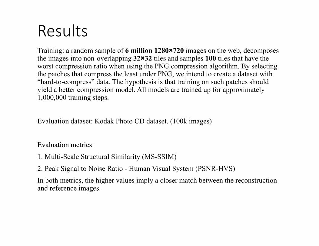
ResultsTraining: a random sample of 6 million 1280×720 images on the web, decomposes the images into non-overlapping 32×32 tiles and samples 100 tiles that have the worst compression ratio when using the PNG compression algorithm. By selecting the patches that compress the least under PNG, we intend to create a dataset with “hard-to-compress” data. The hypothesis is that training on such patches should yield a better compression model. All models are trained up for approximately 1,000,000 training steps.

Evaluation dataset: Kodak Photo CD dataset. (100k images)

Evaluation metrics:

1. Multi-Scale Structural Similarity (MS-SSIM)

2. Peak Signal to Noise Ratio - Human Visual System (PSNR-HVS)

In both metrics, the higher values imply a closer match between the reconstruction and reference images.

ResultsLSTM: Long Short-Term Memory network

GRU: Gated Recurrent Units

MS-SSIM: Multi-Scale Structural Similarity

PSNR-HVS: Peak Signal to Noise Ratio - Human Visual System

AUC: Area Under the rate-distortion Curve

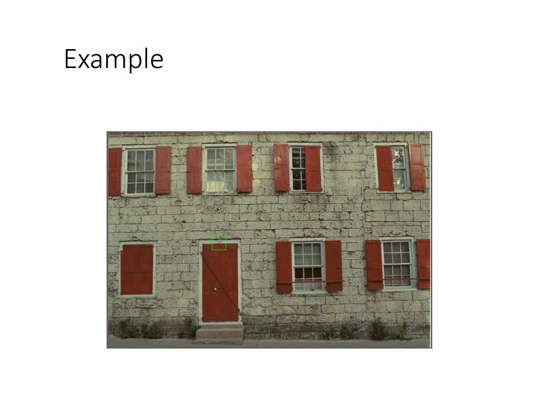
Example

Example

bpp: bits per pixel. Smaller values imply a higher compress ratio.

Example

Original

JPEG420 at 0.5 bpp

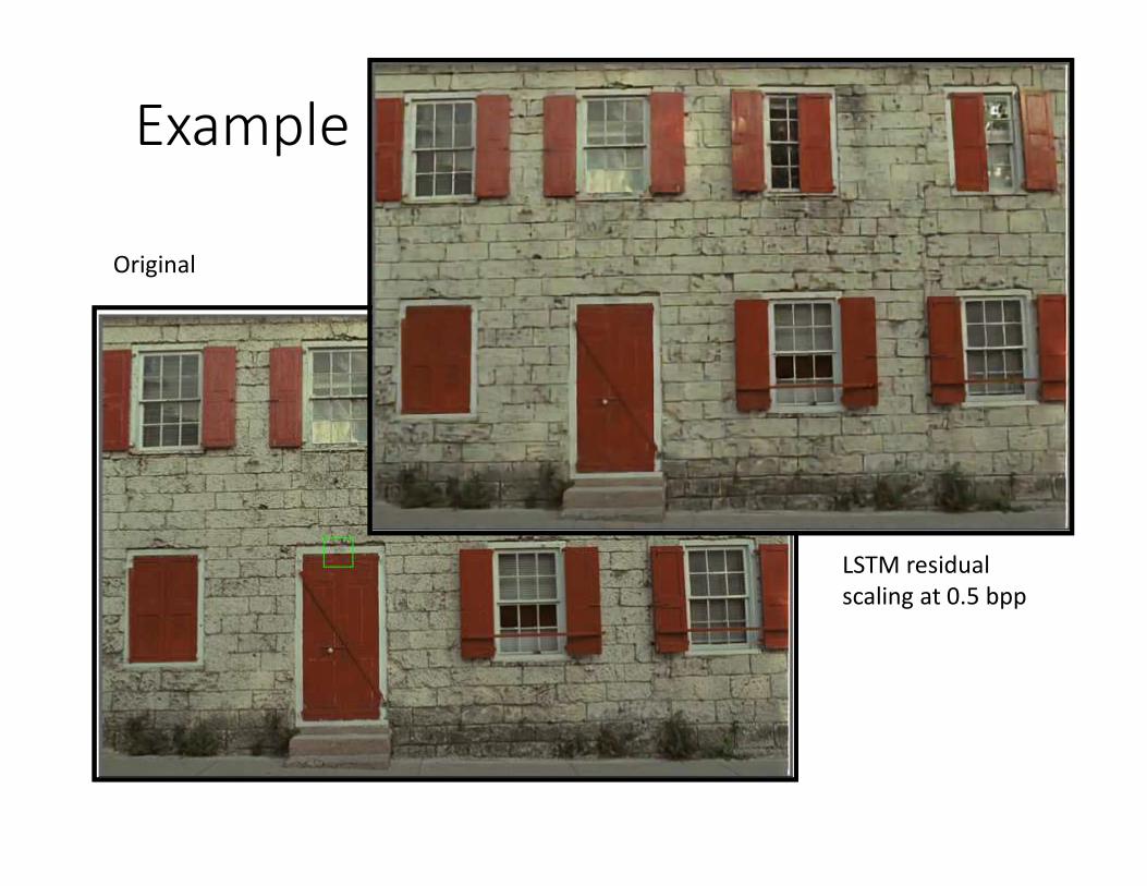
Example

Original

LSTM residual

scaling at 0.5 bpp

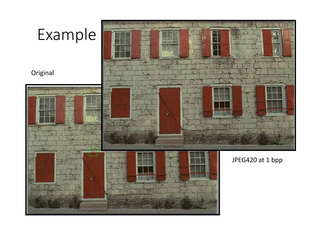
Example

Original

JPEG420 at 1 bpp

Example

Original

LSTM residual

scaling at 1 bpp

Example

Original

JPEG420 at 2 bpp

Example

Original

LSTM residual

scaling at 2 bpp

�Conclusions:

• Presented a RNN based image compression based network.

• This network on average achieve better than JPEG performance over all image size and compression rate.

• Exceptionally good performance on low bit rate compressions.

�Future works:

• Test this method on video compression

• The domain of perceptual difference is still very much in active development. If there is a metric capable of correlating with human raters for all types of distortions, we could incorporate it directly into our loss function, and optimize directly for it.

Thanks for your attention!

• Any questions or comments?

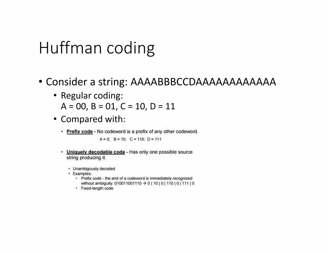
Huffman coding

• Consider a string: AAAABBBCCDAAAAAAAAAAAA

• Regular coding:A = 00, B = 01, C = 10, D = 11

• Compared with:

Convolutional neural network

• Most commonly seen pattern recognition and classification.

• For reference, see: http://cs231n.github.io/convolutional-networks/