FULL REPORT consolidation.docx
35
TITLE : CONSOLIDATION TEST 1.0 INTRODUCTION Consolidation is a process by which soils decrease in volume. According to Karl Terzaghi consolidation is any process which involves decrease in water content of a saturated soil without replacement of water by air. In general it is the process in which reduction in volume takes place by expulsion of water under long term static loads. It occurs when stress is applied to a soil that causes the soil particles to pack together more tightly, therefore reducing its bulk volume. When this occurs in a soil that is saturated with water, water will be squeezed out of the soil. The magnitude of consolidation can be predicted by many different methods. In the Classical Method, developed by Karl von Terzaghi, soils are tested with an odometer test to determine their compression index. This can be used to predict the amount of consolidation. When stress is removed from a consolidated soil, the soil will rebound, regaining some of the volume it had lost in the consolidation process. If the stress is reapplied, the soil will consolidate again along a recompression curve, defined by the recompression index. The soil which had its
-
Upload
fatin-nabihah -
Category
Documents
-
view
1.004 -
download
3
description
report
Transcript of FULL REPORT consolidation.docx

TITLE : CONSOLIDATION TEST
1.0 INTRODUCTION
Consolidation is a process by which soils decrease in volume. According to Karl
Terzaghi consolidation is any process which involves decrease in water content of a
saturated soil without replacement of water by air. In general it is the process in which
reduction in volume takes place by expulsion of water under long term static loads. It
occurs when stress is applied to a soil that causes the soil particles to pack together
more tightly, therefore reducing its bulk volume. When this occurs in a soil that is
saturated with water, water will be squeezed out of the soil. The magnitude of
consolidation can be predicted by many different methods. In the Classical Method,
developed by Karl von Terzaghi, soils are tested with an odometer test to determine
their compression index. This can be used to predict the amount of consolidation.
When stress is removed from a consolidated soil, the soil will rebound, regaining some
of the volume it had lost in the consolidation process. If the stress is reapplied, the soil
will consolidate again along a recompression curve, defined by the recompression index.
The soil which had its load removed is considered to be over consolidated. This is the
case for soils which have previously had glaciers on them. The highest stress that it has
been subjected to is termed the preconsolidation stress. The over consolidation ratio or
OCR is defined as the highest stress experienced divided by the current stress. A soil
which is currently experiencing its highest stress is said to be normally consolidated and
to have an OCR of one. A soil could be considered under consolidated immediately after
a new load is applied but before the excess pore water pressure has had time to
dissipate.

Consolidation is defined as the reduction of the volume of a soil due to the expulsion of
water. This will be accompanied by the dissipation of pore water pressures. A laboratory
consolidation test is performed on an undisturbed sample of a cohesive soil to
determine its compressibility characteristics. The soil sample is assumed to be
representing a soil layer in the ground. A conventional consolidation test is conducted
over a number of load increments. The number of load increments should cover the
stress range from the initial stress state of the soil to the final stress state the soil layer
is expected to experience due to the proposed construction. Increments in a
conventional consolidation test are generally of 24 hr duration and the load is doubled
in the successive increment. In this practical class one load increment of a multi
increment consolidation test is conducted and the data will be analysis to obtain the
compressibility characteristics of the soil.
The compressibility characteristics of the soil are;
(a). Parameters needed to estimate the amount of consolidation settlement
(b). Parameters needed to estimate the rate of consolidation settlement in the field.
Using the data from a single load increment of the test, only the coefficient of volume
compressibility mv can be estimated. Data from all the load increments should be
combined to draw the e vs log σ graph and to obtain the compression index Cc - the
other parameter used to estimate the consolidation settlement. The rate of
consolidation settlement is estimated using the Coefficient of consolidation Cv. This
parameter is determined for each load increment in the test. In this laboratory
assignment, the coefficient of consolidation should be estimated using two methods -
the root time method (Taylor's method) and the log (time) method - Casagrande's
method.

2.0 OBJECTIVE
To determine the consolidation characteristics of soils of low permeability

3.0 THEORY
When a fully saturated soil is subjected to a compressive stress, its volume tends to decrease. The decreasing of its volume is due to compression of the solid grains and escape of water from the voids. In a free drainage soil such as saturated sand the escape of water can take place rapidly. But in clay, due to low permeability, the movement of water occurs very much slowly and therefore, considerable time may be required for excess water to be squeezed out to permeable boundaries.
Settlement is the direct result of the decrease in soil volume and consolidation is the rate of volume decrease with time. The consolidation test is use to estimate the amount of settlement and time of consolidation. From this test some consolidation parameters such as coefficient of consolidation (cv), coefficient of volume compressibility (mv), compression index (Cc), preconsolidation pressure (Pc) can be determined.
There are two methods for determining the coefficient of consolidation:
(i) Casagrande or log (time) or 50% consolidation(ii) Taylor or √ time or 90% consolidation
The coefficient of consolidation can be determined by this equation,
cv=T vH
2
t
Where,
cv = coefficient of consolidation (m2/year)
Tv = Time factor
H = Maximum length of drainage path (m)
t = Time to achieve 50% or 90% consolidation (year or minute)
Figure : Settlement versus log Time
0
5
10
15
20
25
30
0 5 10 15 20 25 30 35 40
Square Root Time (minute)
Set
tlem
ent
(mm
)
x
1.15x
√t90
12

Figure : Settlement versus square root time
4.0 TEST EQUIPMENTS
1. Consolidation apparatus
- Consolidation ring
- Corrossion-resistant porous plate
- Consolidation cell
- Dial Gauge
- Loading device
2. Balance readable to 0.1g
3. Vernier caliper
4. Stop-clock readable to 1 s
0
20
40
60
80
100
120
140
160
0.1 1 10 100 1000 10000
Time (minute)
Set
tlem
ent
(mm
)
100% consolidation line
A
B = 4A
δδ
0% consolidation line
50% consolidation line
t50

5.0 PROCEDURES
1. The internal diameter (D) and the height of the ring was measured by using internal vernier calipers.
2. The ring was weighed to the nearest 0.01g (mR).3. The specimen was cut and was trim into ring.4. The initial moisture content from trimming soil are determined.5. The weight of ring and specimen (m1) are determined.6. The mass of bulk specimen (m) to the nearest 0.01 g was determined using this
equation
m = m1 – mR
7. The consolidation ring and specimen (cutting edge uppermost) was placed centrally on the porous disc.
8. Fit the ring retainer and cell body was fitted and then the upper porous disc was placed centrally on top of the specimen.
9. The consolidation cell was placed centrally in position on the platform of the machine base.
10. The end of the beam are lifted to allow the loading yoke to be raised to the vertical position and the loading stem was adjusted by screwing it downwards until the end engages closely in the recess on the top of the loading cap
11. The compression dial gauge was attached to the arm on the support post.12. Weight (2.5 kg) was added carefully to the load hanger13. Water was added at room temperature to the cell and make sure that the
specimen and upper porous disc are completely submerged. 14. Wind down the beam support and at the same time start the clock. 15. The compression gauge readings and the clock was observed, and the readings
was recorded on a consolidation test form at the selected time intervals.16. The readings of the compression against time to a logarithmic scale and against
square-root-time are plotted.

7.0 RESULTS AND CALCULATION
Date started: 17/2/2011 Sample No: 1
Soil Type: Clay Load: 2.5kg / 50kN/m2
BEFORE TEST
Moisture content for trimming : 60.76 % S.G (Assumed) : 2.7
Weight of ring: 121.0 g Diameter of ring: 75.0 mm
Weight of sample + ring: 265.7 g Area of ring: 4417mm2
Weight of sample: 144.7 g Thickness of ring: 16 mm
Weight of dry sample: 102.6 g Volume of ring : 70672 mm3
Weight of initial moisture: 42.1 g Density, p : 2.05 Mg/m3
Dry density d: 1.45 Mg/m3
Initial void ratio, Gs -1 = 0.862
d
SETTLEMENT READINGS

Elapsed Time
Time (min)
√time
Clock
time
(pm)
Gauge
Reading
Cumulative Compression Hr Min Sec
0 0 0 12.00 0 0
10 0.17 0.41 112 0.22
20 0.33 0.57 120 0.24
30 0.50 0.71 280 0.56
40 0.67 0.82 285 0.57
50 0.83 0.91 300 0.60
1 1 1 12.11 325 0.65
2 2 1.41 12.12 380 0.76
4 4 2 12.14 440 0.88
8 8 2.83 12.18 464 0.92
15 15 3.87 12.25 580 1.16
30 30 5.48 12.40 716 1.43
1 60 7.75 1.10 780 1.56
CALCULATION

Weight of sample = Weight of sample + ring - Weight of ring
= 265.7g – 121.0g
= 144.7g
Weight of initial moisture = Weight of sample - Weight of dry sample
= 144.7g – 102.6 g
= 42.1 g
Initial moisture contents = Weight of initial moisture / Weight of dry sample
= 42.1/102.6
= 0,41 x 100%
= 41%
Area of ring = πD2/4
= π (75.0) 2/4
= 4417 mm 2
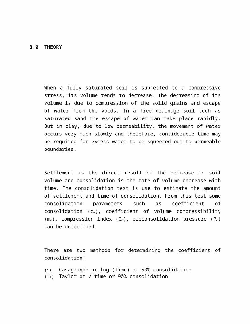
Volume of ring = Area of ring x Thickness of ring
= 4417 x 16
= 70672 mm 3
Density, = Weight of sample (ring)
Volume of ring

= 144.7 x 10 -6 (Mg)
70672 x 10 -9(m3)
= 2.05 (Mg/m 3 )
Dry density, d = Weight of dry sample
Volume of ring
= 102.6 x 10 -6 (Mg)
70672 x 10 -9 (m3)
= 1.45 (Mg/m 3 )
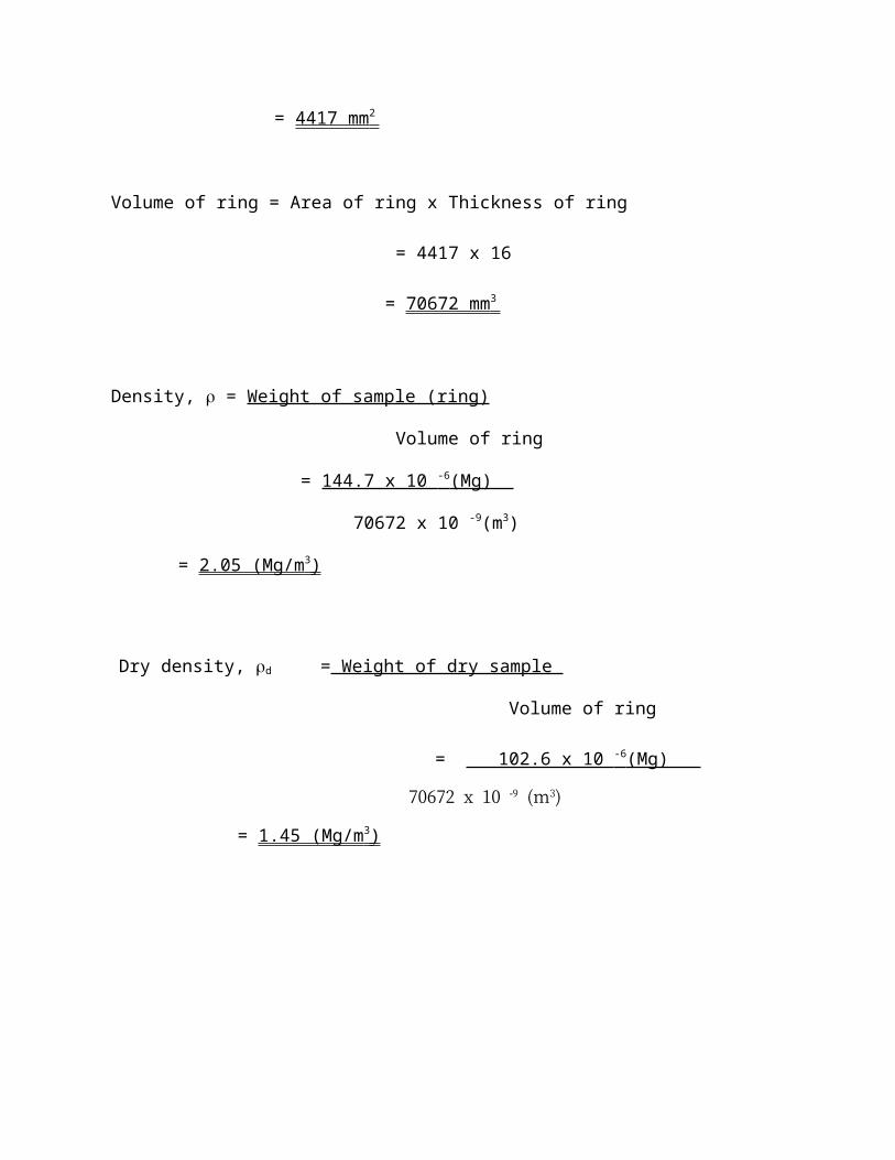
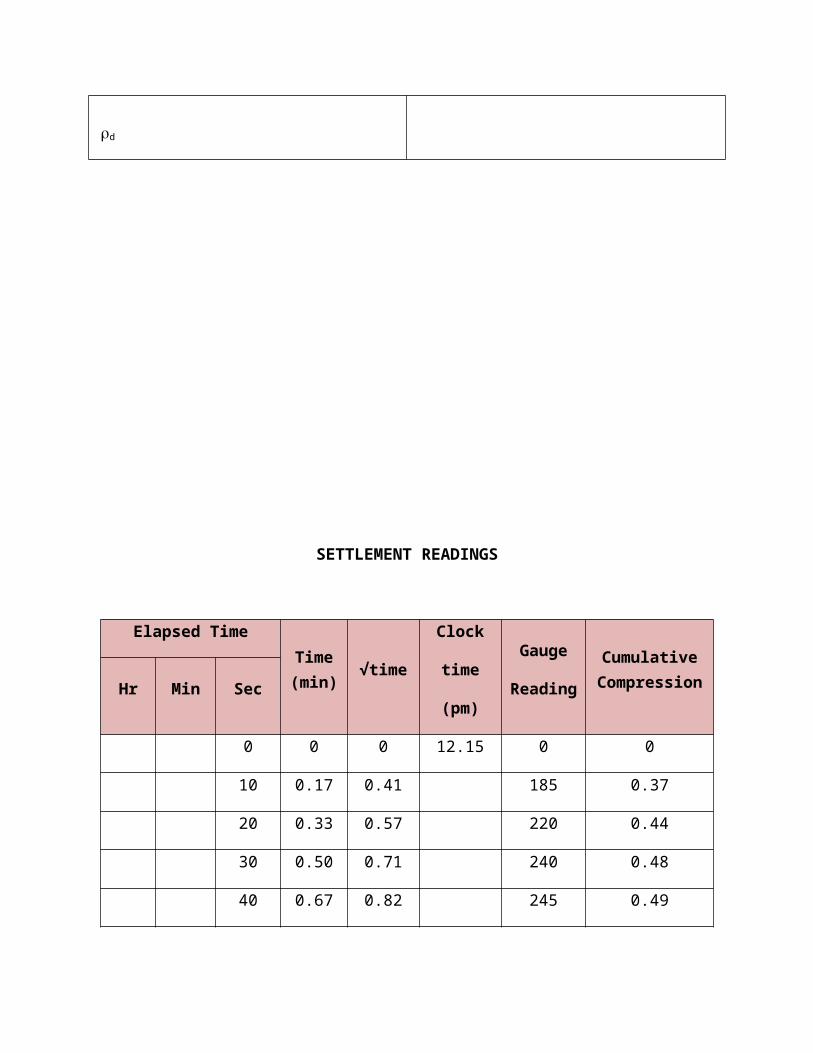
Date started: 17/2/2011 Sample No: 2
Soil Type: Clay Load: 5.0 kg / 100 kN/m2

BEFORE TEST
Moisture content for trimming : 60.76 % S.G (Assumed) : 2.7
Weight of ring: 108.6 g Diameter of ring: 75.0 mm
Weight of sample + ring: 254.0 g Area of ring: 4417mm2
Weight of sample: 145.4 g Thickness of ring: 16 mm
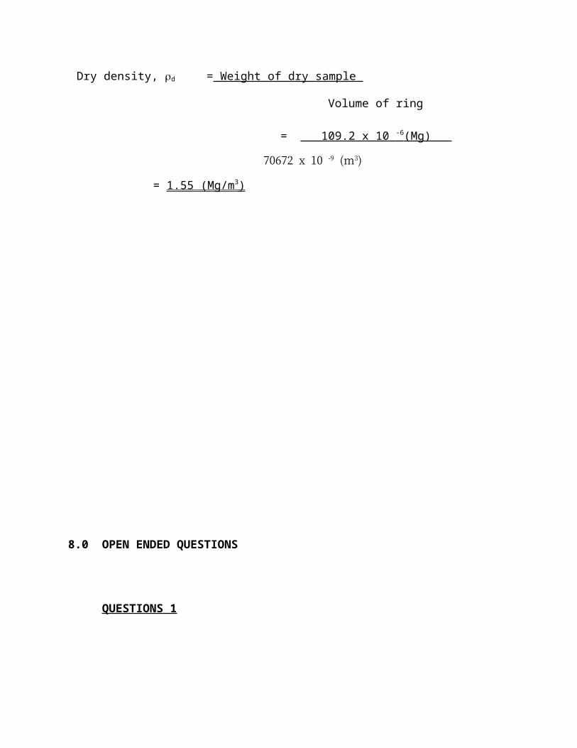
Weight of dry sample: 109.2 g Volume of ring : 70672 mm3
Weight of initial moisture: 36.2 g Density, p : 2.06 Mg/m3
Dry density d: 1.55 Mg/m3
Initial void ratio, Gs -1 = 0.742
d
SETTLEMENT READINGS
Elapsed Time
Time (min)
√time
Clock
time
(pm)
Gauge
Reading
Cumulative Compression Hr Min Sec
0 0 0 12.15 0 0
10 0.17 0.41 185 0.37
20 0.33 0.57 220 0.44
30 0.50 0.71 240 0.48
40 0.67 0.82 245 0.49
50 0.83 0.91 275 0.55
1 1 1 12.16 285 0.57
2 2 1.41 12.17 315 0.63
4 4 2 12.19 403 0.806
8 8 2.83 12.22 521 1.042
15 15 3.87 12.30 656 1.312
30 30 5.48 12.45 666 1.332
1 60 7.75 1.15 682 1.364
CALCULATION
Weight of sample = Weight of sample + ring - Weight of ring
= 254.0g – 108.6g
= 145.4 g
Weight of initial moisture = Weight of sample - Weight of dry sample
= 145.4 g – 109.2 g
= 36.2 g
Initial moisture contents = Weight of initial moisture / Weight of dry sample
= 36.2 /109.2
= 0.331 x 100%
= 33.1%
Area of ring = πD2/4
= π (75.0) 2/4
= 4417 mm 2
Volume of ring = Area of ring x Thickness of ring
= 4417 x 16
= 70672 mm 3
Density, = Weight of sample (ring)
Volume of ring
= 145.4 x 10 -6 (Mg)
70672 x 10 -9(m3)
= 2.06 (Mg/m3)
Dry density, d = Weight of dry sample
Volume of ring
= 109.2 x 10 -6 (Mg)
70672 x 10 -9 (m3)
= 1.55 (Mg/m 3 )
8.0 OPEN ENDED QUESTIONS
QUESTIONS 1

From your experimental data, determine the coefficient of consolidation, cv (m2/year) using Casagrande Method. Please comment your answer.
Sample 1 : Load 2.5 kg (clay soil)
1 10 1000
0.2
0.4
0.6
0.8
1
1.2
1.4
1.6
1.8
Graph settlement versus log time
Time (minute)
Sett
lem
ent (
mm
)
Cv = 0.197 H²
t50
= 0.197 (0.005)²mm

2min
= 4.925 x 10 -6
2
= 2.463 x 10 -6 mm 2 /min
Cv = 2.463 x 10⁻¹³ ( )
= 1.294 x 10 -6 m 2 /year
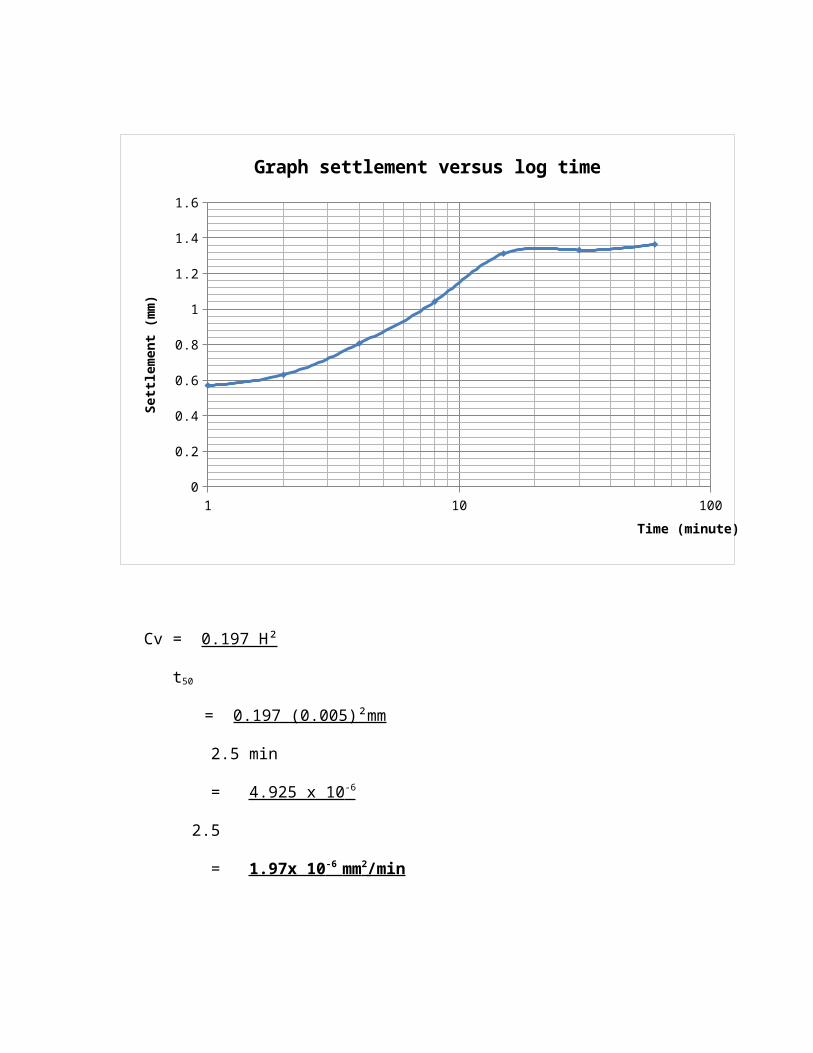
Sample 2 : Load 5.0 kg (clay soil)
1 10 1000
0.2
0.4
0.6
0.8
1
1.2
1.4
1.6
Graph settlement versus log time
Time (minute)
Sett
lem
ent (
mm
)
Cv = 0.197 H²
t50
= 0.197 (0.005)²mm
2.5 min
= 4.925 x 10 -6
2.5
= 1.97x 10 -6 mm 2 /min
Cv = 1.97 x 10⁻¹² ( )

void ratio againts effective stress
0
0.1
0.2
0.3
0.4
0.5
0.6
0.7
0.8
0.9
1
1 10
effective stress , kN/m2
void
ratio
= 1.01 x 10 -6 m 2 /year
2.) Clay samples collected from 5 metres deep in Batu Pahat has a unit weight () of 18
kN/m3. The following data were recorded during an oedometer test.
Effective Stress (kN/m2) 25 50 100 200 400 800 200 50
Void ratio (e) 0.85 0.82 0.71 0.57 0.43 0.3 0.4 0.5
(i) Plot the graph of void ratio against effective stress on semi-log graph and determine the compression index (Cc), Preconsolidation pressure (Pc) and coefficient of volume compressibility (mv)
Cc = slope of the graph = 0.82 – 0.53
The compression index (Cc) is the slope of the graph

log(800/200) = 0.482
From graph, we obtained: Preconsolidation pressure, Pc=150kN/m2
Coefficient of volume compressibility, mv
=
Δe
Δσ '1
1+eavg
Δe
Δσ '=
slope of the graph
eavg=
e1+es2 = (0.85 + 0.5 ) / 2
= 0.675
mv =
Δe
Δσ '1
1+eavg = (0.482) (1/ 1 + 0.675) = 0.288
(ii) Define whether the soil is normally consolidated or over consolidated.
D = 10m
P0= γ×d = 18 ¿ 10 D = 10m = 180kN/m 2
Overconsolidation, OCR=
PcP0
= 150/180 = 0.83 < 1 The soil is over consolidated , OCR<1 . It means that the stress had been applied to the sample of soil previously is less than the stress applied during that test.
QUESTIONS 2
1) From the experimental data , determine the coefficient of consolidation, cv (m2/year)
using Taylor Method. Please comment your answer.
Sample 1 : Load 2.5 kg (clay soil)
1 10 1000
0.2
0.4
0.6
0.8
1
1.2
1.4
1.6
1.8
Cummulative compression VS square root time
Square root ime (minute)
Cum
mul
ative
com
pres
sion
(mm
)
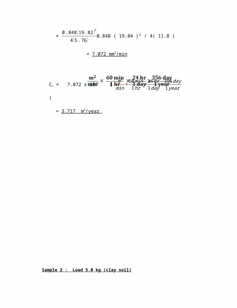
t90 = 11.8

Cv =
= 0.848 ( 19.84 )² / 4( 11.8 )
= 7.072 mm 2 /min
Cv = 7.072 x 10⁻⁶ ( )
= 3.717 m 2 /year
Sample 2 : Load 5.0 kg (clay soil)

1 10 1000
0.2
0.4
0.6
0.8
1
1.2
1.4
1.6
Cummulative compression VS square root time
Square root ime (minute)
Cum
mul
ative
com
pres
sion
(mm
)
t90 = 10.1
Cv =
= 0.848 ( 19.84 )² / 4( 10.1 )
= 8.262 mm 2 /min
Cv = 8.262 x 10⁻⁶ ( )
= 4.343 m 2 /year

2) Clay samples collected from 10 metres deep in Parit Raja has a unit weight () of 20 kN/m3. The following data were recorded during an oedometer test.
Effective Stress (kN/m2) 50 100 200 400 800 1600 400 100
Void ratio (e) 0.95 0.92 0.81 0.67 0.53 0.4 0.5 0.6
(i) Plot the graph of void ratio against effective stress on semi-log graph and determine the compression index (Cc), Preconsolidation pressure (Pc) and coefficient of volume
compressibility (mv).
void ratio againts effective stress
0
0.1
0.2
0.3
0.4
0.5
0.6
0.7
0.8
0.9
1
1 10
effective stress , kN/m2
void
ratio
Cc = slope of the graph
= 0.92 – 0.53

log(800/100)
= 0.408
From graph, we obtained:
Preconsolidation pressure, Pc=150kN/m2
Coefficient of volume compressibility, mv
=
Δe
Δσ '1
1+eavg
Δe
Δσ '=
slope of the graph
eavg=
e1+es2
=0.95+0.62
=0.775
Mv =
Δe
Δσ '1
1+eavg
=(0 .465)( 1
1+0 .775 ) =0.262
(ii) Define whether the soil is normally consolidated or over consolidated.
D = 10m
P0= γ×d
= 20 ¿ 10 D = 10m
= 200kN/m 2
Overconsolidation, OCR=
PcP0
=
150200
= 0.75 < 1
The soil is over consolidated, OCR<1 . It means that the stress had been applied to the
sample of soil previously is less than the stress applied during that test.
9.0 DISCUSSION

Consolidation is a process by which soils decrease in volume. According to Karl
Terzaghi, consolidation is any process which involves decrease in water content of a
saturated soil without replacement of water by air. In general it is the process in which
reduction in volume takes place by expulsion of water under long term static loads. It
occurs when stress is applied to a soil that causes the soil particles to pack together
more tightly, therefore reducing its bulk volume. When this occurs in a soil that is
saturated with water, water will be squeezed out of the soil. The magnitude of
consolidation can be predicted by many different methods. In the Classical Method,
developed by Terzaghi, soils are tested with an oedometer test to determine their
compression index. This can be used to predict the amount of consolidation.
From the experiment that we have done, we have achieved the objective of the
experiment that to determine the consolidation characteristic of soils of flow
permeability. In this experiment we used 2 different weight of slity clay soil which
weighed 2.5 kg for sample 1 and 5.o kg for sample 2.
From the graph settlement versus log time and graph settlement versus square
root time, we get a curve shape for the both sample. From the graph we can find the
value of t50 t90 and other value that is need to calculate the value coefficient of
consolidation, Cv. from the calculation we can see that the value of value coefficient of
consolidation, Cv will increase when the load that we applied to the peat soil ins
increase.

10.0 CONCLUSION
Based on the experiment that we have done, we have determined the consolidation
characteristic of soils of flow permeability through the data that we get after
experiment has finished. Moisture content supply sample silty clay soil is 60.76%. The
coefficient of consolidation, Cv using Casagrande method for Sample 1 is 1.294 x 10⁻⁶
m2/year.
And sample 2 is 1.01 x 10⁻⁶ m2/year. Cv using Taylor method for sample peat soil is 3.717
m2/year and sample clay soil is 4.343 m2/year. Based on the experimental data obtained
in the laboratory, dry density and specific gravity values of tropical peat correlate well.
When large loads such as embankments are applied to the surface, cohesive sub soils
will consolidate, such as settle over time, through a combination of the rearrangement
of the individual particles and the squeezing out of water. The amount and rate of
settlement is of great importance in construction of such structure on a curtain soil area.
For example, an embankment may settle until a gap exists between an approach and a
bridge abutment. The calculation of settlement involves many factors, including the
magnitude of the load, the effect of the load at the depth at which compressible soils
exist, the water table, and characteristics of the soil itself.
11.0 REFERENCES
1. A study on consolidation, shear strength and bearing capacity of soft soil improved by
vertical drain / Farhan Mohammad Ab Latif
2. The study of slag-lime stabilization on consolidation behaviour of Batu Pahat soft clay /
Hemawathy Sathasivam