FULL EMPLOYMENT: ARE WE THERE YET? - Levy ... Bard College Levy Economics Institute Levy Economics...

of Bard College

Levy EconomicsInstitute

Levy Economics Institute of Bard College

Public Policy BriefNo. 142, 2017

FULL EMPLOYMENT: ARE WE THERE YET? flavia dantas and l. randall wray

The Levy Economics Institute of Bard College, founded in 1986, is an autonomous research organization. It is nonpartisan, open to the

examination of diverse points of view, and dedicated to public service.

The Institute is publishing this research with the conviction that it is a constructive and positive contribution to discussions and debates on

relevant policy issues. Neither the Institute’s Board of Governors nor its advisers necessarily endorse any proposal made by the authors.

The Institute believes in the potential for the study of economics to improve the human condition. Through scholarship and research it

generates viable, effective public policy responses to important economic problems that profoundly affect the quality of life in the United

States and abroad.

The present research agenda includes such issues as financial instability, poverty, employment, gender, problems associated with the

distribution of income and wealth, and international trade and competitiveness. In all its endeavors, the Institute places heavy emphasis on

the values of personal freedom and justice.

Editor: Michael Stephens

Text Editor: Barbara Ross

The Public Policy Brief Series is a publication of the Levy Economics Institute of Bard College, Blithewood, PO Box 5000,

Annandale-on-Hudson, NY 12504-5000.

For information about the Levy Institute, call 845-758-7700 or 202-887-8464 (in Washington, D.C.), e-mail [email protected], or visit the Levy

Institute website at www.levy.org.

The Public Policy Brief Series is produced by the Bard Publications Office.

Copyright © 2017 by the Levy Economics Institute. All rights reserved. No part of this publication may be reproduced or transmitted in

any form or by any means, electronic or mechanical, including photocopying, recording, or any information-retrieval system, without

permission in writing from the publisher.

ISSN 1063-5297

ISBN 978-1-936192-54-0

Contents

3 Preface

Jan Kregel

4 Full Employment: Are We There Yet?

Flavia Dantas and L. Randall Wray

21 About the Authors

Levy Economics Institute of Bard College 3

Almost a decade after the Great Recession began, and with

unemployment now at 4.7 percent, many policymakers and

commentators are beginning to lean toward the view that we

have finally reached “full employment”; that any further sig-

nificant improvement in the unemployment rate would lead

to unacceptable increases in inflation. The Federal Reserve has

signaled its resolve to continue tightening monetary policy

through a series of interest rate hikes, and although the new

partisan alignment of Congress and the White House has raised

expectations that fiscal policy might finally be coming off the

sidelines, there is an emerging conventional wisdom that tells

us it is nevertheless “too late” for expansionary federal budgets.

In this policy brief, Flavia Dantas and L. Randall Wray

argue that it is a mistake—and a costly one for society—to

believe that this is what full employment looks like for the US

economy. They contend that we are not even close to the target:

Dantas and Wray estimate we are still roughly 20 million jobs

short of the mark, and that reaching full employment would

require, on average, gains in payroll employment of 420,000

jobs per month for the next four years—or triple the monthly

average we have witnessed since the recovery began.

There are indications that the unemployment rate is over-

stating the health of the labor market. The slow rate of wage

growth and labor compensation in general is indicative of how

far we are from a tight labor market. And while the employment-

to-population ratio has finally been showing signs of modest

improvement, the authors point out that it has increased only 2

percentage points since the recovery began—leaving it well below

its prerecessionary level. This continues an asymmetric trend on

display since 2000, in which the employment ratio declines rap-

idly during recessions and grows much more slowly during recov-

eries, failing to recover prerecession peaks or to match the pace

of the improvement in the U-3 unemployment rate. Recessions

in this millennium have become occasions in which greater and

greater numbers of the population disappear from the labor mar-

ket, “more or less permanently,” the authors observe.

It has become common to attribute this trend to the effect

of demographic or structural forces, such as the aging of the

workforce or a shift in preferences in favor of leisure over labor

(or unpaid household work over paid work). However, Dantas

and Wray point out that these explanations do not adequately

account for the continued erosion of the labor force participa-

tion rate among prime-age workers (ages 25–54). A significant

part of this worrisome trend has been the dramatic erosion

of male prime-age participation rates, but the authors note

that in the current cycle, even female prime-age participation

rates have not recovered their prerecession peaks. The popular

demographic narrative is overstated, they conclude, and has not

been the most important driver of the long-term idling of the

population.

The authors maintain that stagnating incomes and fall-

ing prime-age participation rates are symptoms of a structural

inadequacy of aggregate demand—a problem of insufficient job

creation that has plagued the US economy for some time. It is a

problem, Dantas and Wray emphasize, that conventional public

policy remedies are unable to address.

Their solution to secular stagnation calls for targeted job

creation. Keynesian pump priming, while necessary, is never-

theless too diffuse and not sufficient to counteract the deeper

forces preventing the economy from generating full employ-

ment. A program in which the federal government funds direct

job creation at a uniform minimum wage for all who are willing

and able to work creates the right kind of jobs for the segments

of the population that have been excluded from the labor mar-

ket in recent economic recoveries, while minimizing inflation-

ary pressures.

At this moment, more skepticism is required with regard to

the conventional understanding of full employment, and more

ambition and innovation are needed in devising policies that

ameliorate the lives of those left behind with each successive

economic cycle.

As always, I welcome your comments.

Jan Kregel, Director of Research

February 2017

Preface

Public Policy Brief, No. 142 4

Introduction: Is This as Good as It Gets?

Labor force participation in the United States has declined

continuously since reaching its historical peak in 2000. The

Great Recession accelerated this downward trend as discour-

aged, underemployed, and underpaid workers dropped out

of the labor force. While the employment-to-population ratio

showed some signs of improvement from mid-2015 through

mid-2016, it has recently stagnated. Nonetheless, the Federal

Reserve, much of the media’s pundits, and most policymakers

seem to agree that labor markets have recovered. Official unem-

ployment rates have reached the level that is conventionally

believed to be the lowest that should be pursued, and falling

participation has been widely attributed primarily to structural

forces like age demographics and changing characteristics of the

American labor force. There is no evidence that inflation has

begun to raise its ugly head, but economists inside and outside

the Fed generally agree that interest rates should continue to

rise—to nip price pressures in the bud. In mid-December, the

Fed finally resumed its tightening, and many project four more

hikes over the next year.

While naysayers are in the minority, there is contrary evi-

dence that troubles at least some observers. Most workers have

not seen significant wage increases. And while structural shifts

have partially contributed to the falling participation rate, they

cannot easily explain why participation among prime-age

workers remains significantly below prerecessionary levels. In

particular, there is growing concern that prime-age male labor

force participation is continuing a stubborn long-term down-

ward trend. Further, a few—including Paul Krugman and Larry

Summers—have warned that the nation faces secular stagna-

tion. This is believed to be compounded by growing numbers

of prime-age men who are counted as neither employed nor

unemployed, but as out of the labor force. In addition, growth

of labor productivity has generally been disappointing through-

out the recovery.

To be sure, the two views can be reconciled to produce an

even more dismal prospective future. Our society is aging—

with those at the tip of the baby-boomer iceberg already leav-

ing the labor force as they retire. If we add to that declining

participation in the labor force by the generations currently

of prime age, we face an insufficient supply of workers to pro-

duce the goods and services we need. To some extent, robots

are replacing humans (although it is somewhat puzzling why, if

that were happening on as large a scale as commonly believed,

productivity is not booming). Redundancy of human labor

keeps wage growth low—which further encourages workers to

voluntarily leave the labor market. Hence, we face what looks

like a slack labor market, but one that is tighter than it appears.

Given a constrained labor supply plus slow growth of produc-

tivity, secular stagnation is inevitable.

Some have proposed a basic income guarantee as a solu-

tion to current labor market dynamics: just provide income to

workers who have been displaced by robots, or who do not have

the skills and training required in today’s knowledge economy.

However, that would raise aggregate demand beyond our lim-

ited ability to grow supply-constrained output. The result will

be stagnation and inflation—with the specter of a late-1970s-

style stagflation.

Hence, the conclusion is that this is “as good as it gets.” Even

the current pace of jobs growth is probably too high. It is time to

slow the economy down.

In this policy brief we challenge these views. We will argue

that the slow “recovery” of labor markets, and especially of the

labor force participation rate is due to a combination of insuf-

ficient job creation as well as stagnant wages. The problem is

not really displacement by robots; nor is it a utility-maximizing

choice made by prime-age men to leave the labor force on a

quest for more desirable pursuits; nor is the answer more wel-

fare in the form of a basic income guarantee.

While we do need more aggregate demand, we will argue

that this needs to take the form of targeted job creation as well

as growth of wages at the bottom of the wage ladder. Our rec-

ommendation will follow Hyman Minsky’s “employer of last

resort” proposal that he developed in the 1960s. This would

bring workers back into the labor force without fueling the infla-

tion that would be generated by either the basic income guaran-

tee or the old “Keynesian” reliance on “pump priming”—even

in its modern Trumpian guise of incentivizing infrastructure

investment.

We first provide an overview of recovery of the labor mar-

ket and then turn to longer-term trends. We focus on labor mar-

ket participation, especially of prime-age workers. While female

participation rates had been rising until the early 2000s, partici-

pation by prime-age workers has exhibited a long-term falling

trend. Recessions cause the participation rates of all groups to

fall. In recent expansions, however, the recovery of participation

rates has been attenuated—and in the expansion following the

global financial crisis (GFC), even rates of prime-age females


have not fully recovered. We then turn to a critique of common

explanations of these trends. In that regard, President Obama’s

office released a June 2016 report1 that effectively counters most

of the popular views. We supplement the critique with addi-

tional data and then turn to policy solutions. While the report

offers some helpful suggestions, we find them to be inadequate.

Overview of the Current State of Recovery of

Labor Markets

On December 14, 2016, the Federal Open Market Committee

(FOMC)—the Federal Reserve Bank’s policymaking body—

voted to raise the target range for the federal funds rate from 0.5

percent to 0.75 percent, resuming the “normalization” course

for the Fed funds initiated the previous December. The consen-

sus among FOMC participants is that the US economy is nearly

at full employment, as the official unemployment rate has fallen

below the “normal” levels expected to prevail in the long-run

(some sort of policymakers’ NAIRU—the so-called nonacceler-

ating inflation rate of unemployment).2

Indeed, by important measures there has been substantial

improvement in labor market conditions. A total of 14 million

jobs have been created since the end of the recession. The offi-

cial unemployment rate is now at its lowest level since the GFC,

reaching 4.6 percent in November 2016. Unemployment rates

across different age and demographic groups continue to fall

back toward prerecessionary levels (as can be seen in Figure 1).

And the employment–population ratio that had declined pre-

cipitously after the recession, and has remained unresponsive to

the falling unemployment rate for most of the recovery period,

is finally showing signs of modest improvement (see Figure 2).

While all these developments are welcome, a granular look

at labor markets leads to some caveats to policymakers’ belief

that we’ve achieved full employment. Most importantly, Figure 2

shows that the employment–population ratio is nowhere near

its prerecessionary levels. In the six-and-a-half years since the

ratio stopped falling, it has risen by only 2 percentage points.

At this pace of recovery, it would need more than an addi-

tional dozen years to regain its prerecession peak—an unlikely

scenario.

In fact, since 1990 the pace of recovery of the employment

ratio has been painfully slow after each recession. Perhaps most

concerning is an increasingly asymmetric response of the unem-

ployment rate and the employment ratio over the course of the

cycle: in a downturn the sharp rise of the unemployment rate

is associated with a rapid decline of the employment ratio, but

the relatively sharp fall of unemployment in the recovery is not Figure 1 Unemployment Rates across DifferentDemographic Groups, January 1980 – November 2016

Sources: Bureau of Labor Statistics (BLS); FRED database, Federal ReserveBank of St. Louis

Perc

ent

0

10

20

30

40

50

60

2001

-09

2012

-07

1996

-04

1985

-06

1990

-11

2007

-02

2017

-12

1980

-01

U-3: 16–19 Years of Age, Black

U-3: 16–19 Years of Age, White

U-3: Black

U-3: 20 Years of Age and Older, Black

U-3: Hispanic or Latino

U-3: White

Source: BLS

Perc

ent

3

5

7

9

11

Unemployment Rate (left scale)

Employment–Population Ratio (right scale)

Figure 2 Unemployment Rate and Employment–PopulationRatio, 1989–2016

2001

-01

2007

-01

1998

-01

1992

-01

1995

-01

2004

-01

2013

-01

2010

-01

1989

-01

56

58

60

62

66

64

2016

-01


matched by a quick restoration to a higher employment ratio.

All else equal, a falling unemployment rate should increase the

employment–population ratio as those searching for jobs are

finding them with greater success. As Figure 2 shows, however,

recovery of the employment ratio is increasingly difficult. This is

because a greater proportion of the unemployed are leaving the

labor force rather than finding jobs, as was the case before 1990.

When a smaller percentage of the working-age civilian popula-

tion is participating in the labor market, falling unemployment

does not necessarily increase the employment–population ratio.

Figure 2 shows that while the unemployment rate has fallen by

5 percentage points over the recent recovery, the employment

rate has risen by only 2 percentage points. By contrast, in the

recovery of the early 1990s, the unemployment rate fell by about

3.5 percentage points, while the employment rate rose by about

the same number of percentage points.

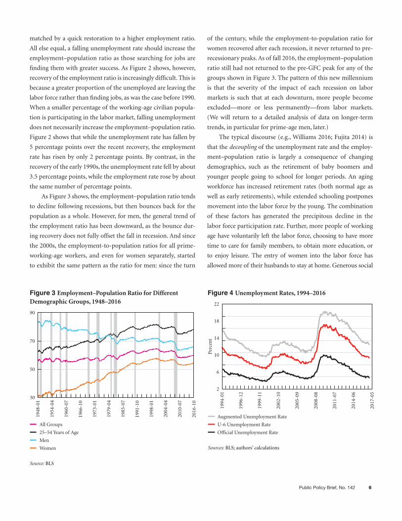
As Figure 3 shows, the employment–population ratio tends

to decline following recessions, but then bounces back for the

population as a whole. However, for men, the general trend of

the employment ratio has been downward, as the bounce dur-

ing recovery does not fully offset the fall in recession. And since

the 2000s, the employment-to-population ratios for all prime-

working-age workers, and even for women separately, started

to exhibit the same pattern as the ratio for men: since the turn

of the century, while the employment-to-population ratio for

women recovered after each recession, it never returned to pre-

recessionary peaks. As of fall 2016, the employment–population

ratio still had not returned to the pre-GFC peak for any of the

groups shown in Figure 3. The pattern of this new millennium

is that the severity of the impact of each recession on labor

markets is such that at each downturn, more people become

excluded—more or less permanently—from labor markets.

(We will return to a detailed analysis of data on longer-term

trends, in particular for prime-age men, later.)

The typical discourse (e.g., Williams 2016; Fujita 2014) is

that the decoupling of the unemployment rate and the employ-

ment–population ratio is largely a consequence of changing

demographics, such as the retirement of baby boomers and

younger people going to school for longer periods. An aging

workforce has increased retirement rates (both normal age as

well as early retirements), while extended schooling postpones

movement into the labor force by the young. The combination

of these factors has generated the precipitous decline in the

labor force participation rate. Further, more people of working

age have voluntarily left the labor force, choosing to have more

time to care for family members, to obtain more education, or

to enjoy leisure. The entry of women into the labor force has

allowed more of their husbands to stay at home. Generous social

Figure 3 Employment–Population Ratio for DifferentDemographic Groups, 1948–2016

Source: BLS

30

50

70

All Groups

25–54 Years of Age

Men

Women

1973

-01

1985

-07

1966

-10

1954

-04

1960

-07

1979

-04

1998

-01

1991

-10

1948

-01

90

2004

-04

2016

-10

2010

-07

Figure 4 Unemployment Rates, 1994–2016

Sources: BLS; authors’ calculations

Perc

ent

2

6

10

14

18

22

Augmented Unemployment Rate

U-6 Unemployment Rate

Official Unemployment Rate

1996

-12

2011

-07

2002

-10

2008

-08

2005

-09

1994

-01

2017

-05

2014

-06

1999

-11


safety nets reduce the costs of exit from the labor force. Skills mis-

match make such exits by prime-age men more appealing than

taking a job that requires little skill and pays much lower wages.

Figure 4 plots the official unemployment rate against the

“unofficial” U-6 measure provided by the Bureau of Labor

Statistics (BLS),3 which includes not only those who are mar-

ginally attached4 to the labor force but also those who are

employed part time for economic reasons (i.e., cannot find full-

time employment). As of November 2016, the U-6 unemploy-

ment rate was 9.3 percent. There were still 7.4 million people

unemployed, 5.5 million people employed part time for eco-

nomic reasons, and 1.9 million people marginally attached to

the labor force. Only 228,000 were marginally attached due to

school or training, and only 176,000 were marginally attached

due to illness or disability. The vast majority of the marginally

attached were discouraged (could not find a job) or out of the

labor force for other factors that made participation prohibi-

tive, including childcare and transportation difficulties.5 This is

not surprising, given the difficulty of accessing affordable, avail-

able, and adequate childcare6 and public transportation.

However, even the U-6 measure of unemployment is likely

to understate the challenges we still face today, because the BLS

statistics consider “marginally attached” only those who have

searched for employment in the previous year. In November

2016, according to the BLS, there were 5.9 million people out-

side of the labor force who reported wanting a job now,7 3.4

million of whom had not searched for work in the previous

year. Taking these people into account, a more comprehensive

measure boosts the unemployment rate to 12 percent, a mea-

sure labeled Augmented Unemployment8 in Figure 4.

Adding the number of people who were unemployed in

November 2016 to the number of those who were employed

part time for economic reasons, plus those not in the labor force

who want a job now, minus those who are not available to work

now (ill, disabled, or in school), provides an estimate of 20 mil-

lion potential workers who are at least partially idled.

The US economy created on average 180,000 jobs per

month from January to November 2016. This represents a

slowdown from the monthly average of 225,000 in 2015, and

248,000 in 2014. To achieve the same employment–popu-

lation ratio that prevailed before the recession, Carnevale,

Jayasundera, and Gulish (2015) estimate that the US economy

would need to create on average 204,000 jobs per month over

the next four years. To accommodate all those who are part of

the U-6 measure of labor underutilization, the required aver-

age job creation per month jumps to 309,000 for the next four

years. And finally, to accommodate all those included in our

Augmented Unemployment figure, a total of 420,000 jobs per

month over the next four years would be necessary.

In sum, almost a decade after the United States’ worst down-

turn since the Great Depression, we still have not fully recovered.

The costs to individuals and society of labor underutilization

(unemployment plus underemployment) come in the form

of huge net income and output losses that may be permanent.

The social costs are even larger, and include: poverty, social

isolation, and crime; regional deterioration; health issues,

family breakdown, and school dropouts; social, political, and

economic instability; promotion of violence, ethnic hostility,

and even terrorism; and loss of human capital.

Many of these problems combine to push workers out of

the labor market. Further, there are hysteresis effects, as the

long-term unemployed (as well as those who are out of the

labor force for extended periods) become unemployable—at

least in the eyes of potential employers.

On the other hand, full employment provides a large num-

ber of benefits, including: production of goods and services;

on-the-job training and skills development; poverty alleviation;

community building and social networking; intergenerational

stability; and social, political, and economic stability.

As Sen (1999) argues, full employment generates multiplier

effects, as positive feedbacks and reinforcing dynamics cre-

ate a virtuous cycle of socioeconomic benefits. We thus con-

tinue to incur huge costs and fail to achieve the benefits of full

employment.

As we will argue in the next section, longer-term trends

have made it much more difficult to achieve anything close to

full employment.

Longer-term Trends in Labor Force Participation

Rates

Falling Participation by Prime-age Men: Demographic

Reasons

As workers who still want jobs leave the labor force (stop actively

searching for employment in the previous four weeks), the

labor force participation rate (LFPR)9 is depressed. The LFPR

(and also the employment–population ratio) has been declin-

ing since it reached its historical peak in 2000. By 2015, the ratio


reached its lowest level since 1977—62.4 percent. The recession

accelerated the downward trend as discouraged and underem-

ployed workers dropped out of the labor force, but it cannot

easily explain why this ratio has been falling since the start of

the new millennium.

The typical explanation for declining labor force participa-

tion is age demographics, combined with changing character-

istics of the American labor force and other structural forces

(see, e.g., Aaronson et al. 2006; Eberstadt 2016). For example, as

the American population gets older, all else equal, overall labor

force participation naturally declines, pulled by the lower par-

ticipation rate for those aged 55 and older, at the same time that

their share of the population increases. Similarly, as the percent-

age of the population of prime working age (typically an age

group with a higher LFPR) declines, so does overall labor force

participation.

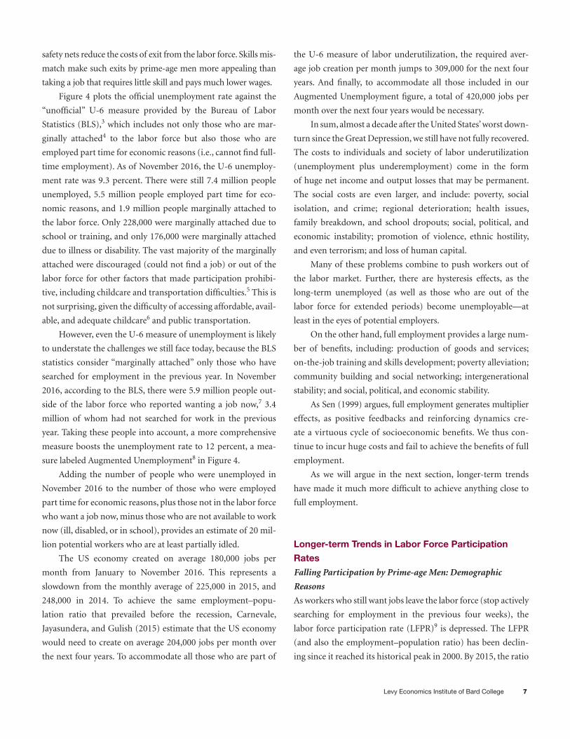
However, as can be seen in Figure 5, labor force participa-

tion for those 55 and older has actually been rising (although

the rate might have leveled off in the past few years), partially

counteracting the negative impact of an aging population on

the overall LFPR.10 A puzzling trend is that labor force partici-

pation has been declining since 2000 for those of prime working

age, that is, those between 25 and 54 years of age.11 Participation

rates have also fallen for younger age groups.

Figure 6 shows the weighted contribution of prime-age

workers and older workers as a percentage of the overall LFPR.

As can be seen below, the relative importance of workers aged

55 and older in the total LFPR has been increasing, while the

relative importance of the prime-age group to the total LFPR

has actually declined.

While many attribute the falling participation rate to aging

of the population (as the average age of workers rises, the

Figure 5 LFPRs for Different Age Groups, 1980–2016

Source: BLS

Perc

ent

55

30

40

50

60

70

80

90

16–19 (right scale)

20–24 (left scale)

25–54 (left scale)

55 and Older (right scale)

2001

-01

2011

-07

1995

-10

1985

-04

1990

-07

2006

-04

2016

-10

1980

-01

Perc

ent

20

60

65

75

85


Perc

ent

-25

0

25

50

75

100

Percent Decline: Age Demographics

Percent Decline: Non-age-related Factors

2010

-07

2008

-01

2009

-04

Figure 7 Decomposing Causes of the Decline in the LFPR,January 2008 – October 2016

2014

-02

2011

-10

2013

-01

2016

-10

2015

-07


Perc

ent

16

18

20

22

24

Relative Importance: 25–54 (right scale)

Relative Importance: 55 and Older (left scale)

Figure 6 Weighted Contribution for Selected Age Groups(as a percentage of the overall LFPR), December 2007 – October 2016

2013

-12

2016

-12

2012

-06

2007

-12

2010

-12

2015

-06

2009

-06

Perc

ent

63

65

67

69


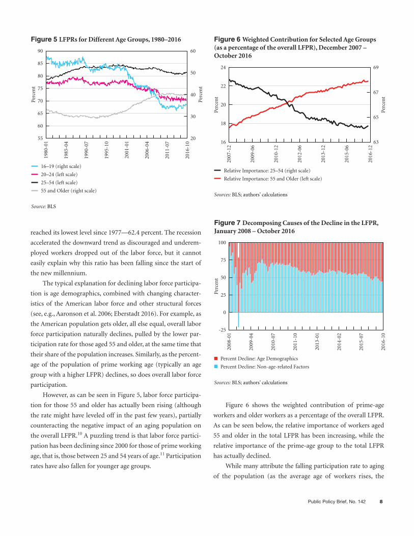
participation rate falls), that effect is overstated. Following

Mitchell (2014), a simple exercise can provide a rough estimate

of the percentage of the decline in the overall LFPR over the

period January 2008 to October 2016 that can be attributed to

aging. The results are plotted in Figure 7. Briefly, the time series

is constructed by holding constant the proportion of the differ-

ent age groups in the CNIP (civilian noninstitutional popula-

tion) as of January 2008 (the month following the official start

of the recession), and allowing the LFPR for each age group to

vary over time. As the population ages, the overall LFPR tends to

fall because of the increase in the relative weight of the CNIP of

workers above 55 (who have a lower LFPR). Keeping the CNIP

constant allows one to estimate what the LFPR would have been

had age demographics not changed over that time period.

Using the constructed time series, Figure 7 shows the per-

cent of the cumulative decline in the LFPR from January 2008

that was due to changes in age demographics (red bars) and to

all other factors (blue bars). For example, in October 2016 the

actual LFPR was 62.8 percent, representing a total decline of

3.4 percentage points from January 2008, when the LFPR was

66.2. Our constructed LFPR series tells us that in the absence

of changing age demographics, the LFPR would have been 64.7

percent. In other words, 44 percent of the total decline in the

labor force from January 2008 was due to non-age-related fac-

tors. This represents a decline of 3.8 million people in the labor

force for non-age-related reasons. From the official end of the

recession (June 2009) to today, the non-age-related decline in

labor force participation explains on average around 60 percent

of the decline in the LFPR. Our estimation is in line with other

studies.12

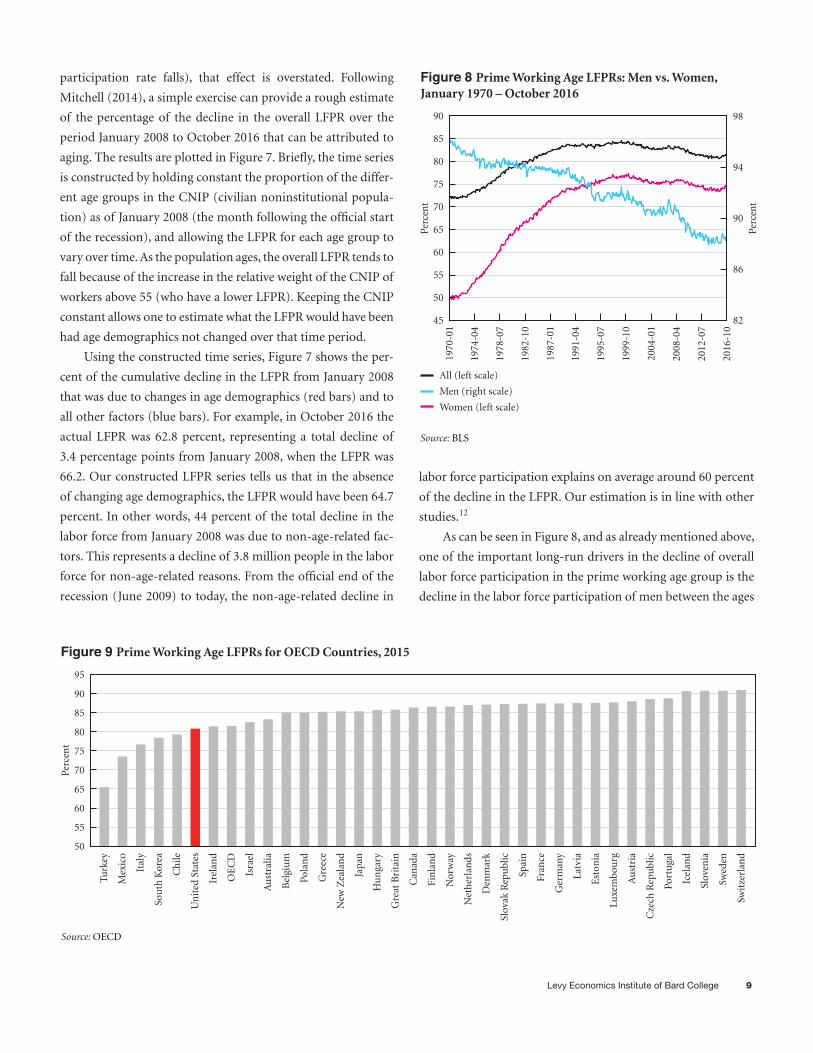
As can be seen in Figure 8, and as already mentioned above,

one of the important long-run drivers in the decline of overall

labor force participation in the prime working age group is the

decline in the labor force participation of men between the ages

Source: BLSPe

rcen

t

45

50

55

60

65

70

85

90

All (left scale)

Men (right scale)

Women (left scale)

Figure 8 Prime Working Age LFPRs: Men vs. Women,January 1970 – October 2016

1987

-01

1995

-07

1982

-10

1974

-04

1978

-07

1991

-04

2004

-01

1999

-10

1970

-01

Perc

ent

82

86

90

94

98

75

80

2008

-04

2016

-10

2012

-07

Figure 9 Prime Working Age LFPRs for OECD Countries, 2015

Source: OECD

Perc

ent

60

65

70

75

80

85

90

95

Bel

giu

m

Irel

and

Sou

th K

orea

Mex

ico

Ital

y

Isra

el

Ch

ile

Un

ited

Sta

tes

Turk

ey

50

55

Nor

way

Can

ada

Japa

n

Gre

ece

New

Zea

lan

d

Fin

lan

d

Hu

nga

ry

Gre

at B

rita

in

Pola

nd

Spai

n

Den

mar

k

Slov

ak R

epu

blic

Net

her

lan

ds

Icel

and

Cze

ch R

epu

blic

Est

onia

Ger

man

y

Lat

via

Port

uga

l

Luxe

mbo

urg

Au

stri

a

Fran

ce

Swit

zerl

and

Slov

enia

Swed

en

Au

stra

lia

OE

CD


of 25 and 54. The erosion of labor force participation for men of

prime working age has been steady in the US economy since the

mid-1960s. Eberstadt (2016), for example, calculates that today,

“a monthly average of nearly one in six prime-age men [has] no

paying job of any kind” (Eberstadt 2016, 213). If current trends

continue, in 40 years, one out of four men of prime working age

will be out of the labor force (Summers 2016). Labor force par-

ticipation rates have declined across the board for men of prime

age, but the fall has been steeper for black men, those convicted of

crimes, those with a high school degree or less, and those without

dependents or children (CEA 2016; Eberstadt 2016).

The United States does not fare well in international

comparisons: in 2015 it had one of the lowest labor force

participation rates among OECD (Organisation for Economic

Co-operation and Development) countries, as can be seen in

Figure 9. It is hard to make the argument that excessive labor

market regulation or a generous social safety net is the reason

for the lower participation rates in the United States compared

with OECD countries, since those countries generally have

labor markets that are more regulated, as well as social safety net

schemes that are more extensive and comprehensive. Further,

since the US Congress passed the Personal Responsibility and

Work Opportunity Reconciliation Act in 1996—which cur-

tailed or imposed time limits on government assistance to those

in need in order to promote private sector work over govern-

ment dependency of the able-bodied—the participation rate

has actually declined, in contrast to other OECD countries, as

can be seen in Figure 10. The United States is among only a

handful of countries with a falling participation rate.

Falling Participation of Prime-age Men: Labor Market

Supply-Side Explanations

Some have attributed the decline of labor force participation

to “social shifts” such as changes in personal preferences, lead-

ing more people to trade “a second paycheck for spending more

time at home, whether it’s for child care, leisure, or simply that

it’s a better lifestyle fit,” according to Williams (2016, 3), or

to seek higher educational achievement. While the decline of

labor force participation for those between the ages of 16 and

24 reflects the fact that Americans are spending more years in

school, it cannot explain why Americans of prime working age

have simply withdrawn from the labor market.

While the social shifts explanation sounds plausible, it is

unlikely that a large number of Americans are voluntarily leav-

ing the labor force for personal preferences. In fact, the number

of those not in the labor force who report not wanting a job now

has declined for age groups 16–24 and 25–54.13 Further, the his-

torical trend for married couples with children under 18 shows

a significant increase in the percentage of families in which both

parents are employed—from 25 percent in the 1960s to almost

61 percent in May 2016. Neither of these trends is obviously

consistent with the “lifestyle changes” argument.

The number of men of prime working age who are neither

employed nor looking for a job has more than doubled over the

Sources: OECD; authors’ calculations

Figure 10 Change in Prime Working Age LFPRs for OECD Countries, 1990–2015

Perc

ent

0

5

10

15

20

Bel

giu

m

Irel

and

Sou

th K

orea

Ital

y

Isra

el

Un

ited

Sta

tes

Turk

ey

-5

Nor

way

Can

ada

Japa

n

Gre

ece

New

Zea

lan

d

Gre

at B

rita

in

Den

mar

k

Net

her

lan

ds

Ger

man

y

Port

uga

l

Luxe

mbo

urg

Fran

ce

Swed

en

Au

stra

lia

OE

CD

Fin

lan

d

Spai

n

Est

onia


past 50 years (Eberstadt 2016). According to the president’s June

2016 report, adverse labor supply conditions explain very little

of this decline—fewer than 25 percent of prime-age people who

are not participating in the labor force have a working spouse,

and nearly 36 percent of them were living in poverty (CEA

2016). The report also shows that “prime-age males without

children saw a larger decline of 9.4 percentage points since 1968

compared to 4.9 percentage points among prime-age males

with children” (CEA 2016, 14). That runs counter to the belief

that the “supply side” choice to leave the labor force to take care

of children can explain much of the movement of prime-age

men out of the labor force. Only a quarter of prime-age men

who are not in the labor force are parents, falling from 40 per-

cent in 1968 (CEA 2016).

Further, the falling participation rate of prime-age men

is limited to native-born Americans—participation rates of

immigrants have risen since 1994 (CEA 2016). And the chal-

lenges military veterans face in the labor market cannot explain

much of it either, because the share of prime-age men out of the

labor force who are veterans has been declining. Some of those

who are out of the labor force participate in under-the-table

work, but there’s no evidence that the “shadow” economy has

increased in recent years relative to the economic activity from

which reported data draw.

The data also cast doubt on the argument that prime-age

men are leaving the labor force to collect generous social benefits

such as welfare and disability pay.14 In the 1970s, “cash welfare

income was the largest source of income, on average, for house-

holds with prime-age men not participating in the workforce,”

but with reductions of the social safety net, welfare has become

relatively unimportant (CEA 2016, 19). Social Security is the

biggest source of government-provided income (almost a quar-

ter of prime-age men out of the labor force receive some), with

Supplemental Security Income15 payments going to 15 percent

of such men. Disability insurance (SSDI) now goes to about 3

percent of prime-age men (triple the percentage in 1967), but

that is not nearly enough to explain the falling participation

rates. The president’s report estimates it might explain 0.3–0.5

percentage points of the 7.5 percentage point decline since 1967

(CEA 2016, 20). So while some types of government income

supports (Social Security, SSI, SSDI) have seen increasing use,

this has been largely offset by a decline in the use of “welfare”

(today, Temporary Assistance for Needy Families, or TANF) and

food stamps (now called SNAP—the Supplemental Nutrition

Assistance Program). It is true that prime-age men who are out

of the labor force make greater use of these programs than those

who are working, but the important point is that restrictions

have reduced the benefits paid through these programs—which

is hardly an explanation for increasing rates of nonparticipation

in the labor force. Note also that wealthy OECD nations—with

better social safety nets—have not seen participation rates fall.

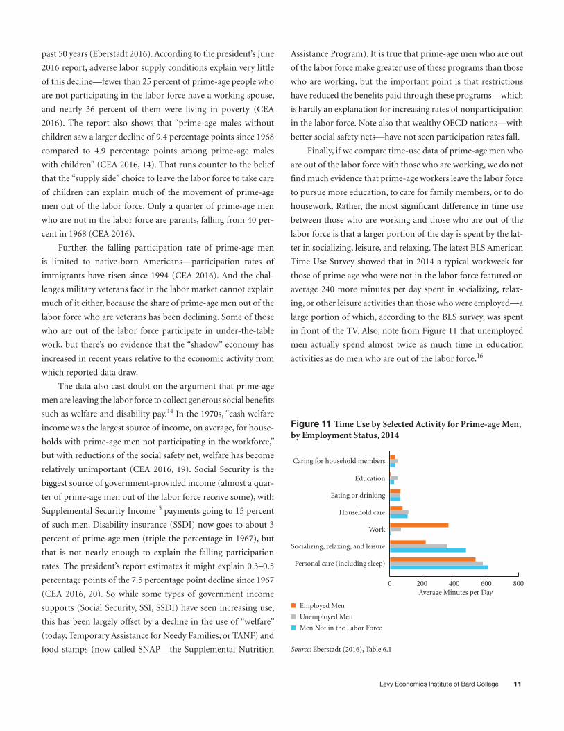
Finally, if we compare time-use data of prime-age men who

are out of the labor force with those who are working, we do not

find much evidence that prime-age workers leave the labor force

to pursue more education, to care for family members, or to do

housework. Rather, the most significant difference in time use

between those who are working and those who are out of the

labor force is that a larger portion of the day is spent by the lat-

ter in socializing, leisure, and relaxing. The latest BLS American

Time Use Survey showed that in 2014 a typical workweek for

those of prime age who were not in the labor force featured on

average 240 more minutes per day spent in socializing, relax-

ing, or other leisure activities than those who were employed—a

large portion of which, according to the BLS survey, was spent

in front of the TV. Also, note from Figure 11 that unemployed

men actually spend almost twice as much time in education

activities as do men who are out of the labor force.16

Source: Eberstadt (2016), Table 6.1

0

Personal care (including sleep)

Socializing, relaxing, and leisure

Work

Household care

Eating or drinking

Education

Caring for household members

Average Minutes per Day

Figure 11 Time Use by Selected Activity for Prime-age Men,by Employment Status, 2014

800400 600200

Employed Men

Unemployed Men

Men Not in the Labor Force


Falling Participation Rates: Demand-side and

Institutional Factors

The president’s report credits demand-driven and institutional

factors for much of the decline in the participation rate of

prime-age men. The additional reasons for falling participation

rates examined in the report are:

Falling demand for middle- and low-skilled workers:

Unsurprisingly, participation has fallen steeply for

less-educated men at the same time that the demand-

driven wage differential between more educated and

less-educated men has increased. Using wage pres-

sure as a proxy for demand, and educational achieve-

ment as proxy for skills, the report finds that lack of

demand for middle- and low-skilled workers has been

an important driver of falling participation.

Lack of jobs at decent wages: Related to the falling

demand argument above is the relative decline in

wages for low-skilled workers. As wage and income

inequality increase, labor force participation for those

at the bottom of the income distribution declines. In

fact, state-level data used by the President’s Council

of Economic Advisers (CEA) suggest that the corre-

lation between labor force participation and relative

wages is the strongest for this group. According to their

estimates, “at the 10th percentile, a $1,000 increase in

annual wages, or a roughly $0.50 increase in hourly

wages for a full-time, full-year worker, is associated

with a 0.13 percentage-point increase in the State par-

ticipation rate for prime-age men” (CEA 2016, 3).

While we find many of these supply-side, demand-side, and

institutional factors important, we believe that the president’s

report, as well as most other analyses, is deficient. None have

placed sufficient emphasis on overall economic performance, as

they generally presume that we have, indeed, “recovered.” We

disagree, as we think that the economy remains far from full

employment. Let us turn to an alternative explanation. We will

argue that the main problem is insufficient demand, and that

the solution to rising long-term unemployment and labor force

exit is targeted job creation.

How Close Are We to Full Employment? Evidence

from Wage Pressures

Labor Incomes

Perhaps the clearest evidence that the US economy is far from

full employment is the slow rate of growth of wages and over-

all labor compensation. In a healthy economy, full employment

should translate into higher real wage growth as labor becomes

relatively scarce, assuming everything else remains constant. As

Figure 12 shows, however, nonfarm nominal average hourly

earnings have not yet returned to precrisis levels. In the post-

recession period, nominal hourly earnings have increased on

average 2.11 percent per year. And despite low unemployment

rates, earnings increased at an annualized average of 2.45 per-

cent in November 2016, which is low when taking into account

productivity growth plus inflation.

It is now widely known that growth in real hourly com-

pensation has significantly lagged behind labor productivity

(this phenomenon is known to conventional economists as

the productivity puzzle). Standard economic theory suggests

that real wages over time tend to increase with labor produc-

tivity—the assumption is that under full employment, work-

ers and employers approach the bargaining process with more

equal power so that each walks away from the production pro-

cess fairly compensated for their contribution. In fact, this is the

assumption behind the models used by the Fed to predict future

labor trends.

Sources: BLS; National Bureau of Economic Research (NBER)

Perc

ent

Incr

ease

0

2

4

6

8

10

All Nonfarm Employees

Production/Nonsupervisory Workers

2000

-01

1995

-01

1990

-01

1980

-01

1985

-01

2005

-01

Figure 12 Nonfarm Private Sector Nominal Hourly WageGrowth, 1980–2016 (year-on-year)

2010

-01

2015

-01


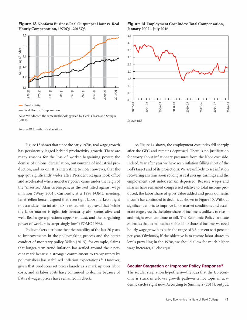
Figure 13 shows that since the early 1970s, real wage growth

has persistently lagged behind productivity growth. There are

many reasons for the loss of worker bargaining power: the

demise of unions, deregulation, outsourcing of industrial pro-

duction, and so on. It is interesting to note, however, that the

gap got significantly wider after President Reagan took office

and accelerated when monetary policy came under the reign of

the “maestro,” Alan Greenspan, as the Fed tilted against wage

inflation (Wray 2004). Curiously, at a 1996 FOMC meeting,

Janet Yellen herself argued that even tight labor markets might

not translate into inflation. She noted with approval that “while

the labor market is tight, job insecurity also seems alive and

well. Real wage aspirations appear modest, and the bargaining

power of workers is surprisingly low” (FOMC 1996).

Policymakers attribute the price stability of the last 20 years

to improvements in the policymaking process and the better

conduct of monetary policy. Yellen (2015), for example, claims

that longer-term trend inflation has settled around the 2 per-

cent mark because a stronger commitment to transparency by

policymakers has stabilized inflation expectations.17 However,

given that producers set prices largely as a mark up over labor

costs, and as labor costs have continued to decline because of

flat real wages, prices have remained in check.

As Figure 14 shows, the employment cost index fell sharply

after the GFC and remains depressed. There is no justification

for worry about inflationary pressures from the labor cost side.

Indeed, year after year we have seen inflation falling short of the

Fed’s target and of its projections. We are unlikely to see inflation

recovering anytime soon so long as real average earnings and the

employment cost index remain depressed. Because wages and

salaries have remained compressed relative to total income pro-

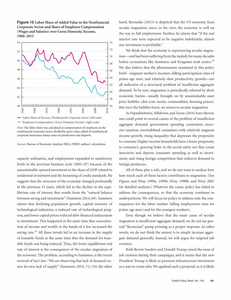
duced, the labor share of gross value added and gross domestic

income has continued to decline, as shown in Figure 15. Without

significant efforts to improve labor market conditions and accel-

erate wage growth, the labor share of income is unlikely to rise—

and might even continue to fall. The Economic Policy Institute

estimates that to maintain a stable labor share of income, we need

hourly wage growth to be in the range of 3.5 percent to 4 percent

per year. Obviously, if the objective is to restore labor shares to

levels prevailing in the 1970s, we should allow for much higher

wage increases, all else equal.

Secular Stagnation or Improper Policy Response?

The secular stagnation hypothesis—the idea that the US econ-

omy is stuck in a lower growth path—is a hot topic in aca-

demic circles right now. According to Summers (2014), output,

Source: BLS

0.0

1.5

2.0

2.5

3.0

3.5

4.0

4.5

2010

-05

2008

-04

2006

-03

2002

-01

2004

-02

2012

-06

Figure 14 Employment Cost Index: Total Compensation,January 2002 – July 2016

0.5

1.0

2014

-07

2016

-08


Nat

ura

l Log

of

Inde

x

4.5

4.7

4.9

5.1

5.3

5.5

Productivity

Real Hourly Compensation

1992

Q1

1986

Q3

1981

Q1

1970

Q1

1975

Q3

1997

Q3

Figure 13 Nonfarm Business Real Output per Hour vs. RealHourly Compensation, 1970Q1–2015Q3

Note: We adopted the same methodology used by Fleck, Glaser, and Sprague(2011).

2003

Q1

2008

Q3

2014

Q1


capacity utilization, and employment expanded to satisfactory

levels in the previous business cycle (2001–07) because of the

unsustainable upward movement in the share of GDP related to

residential investment and the loosening of credit standards. He

suggests that the structure of the economy changed profoundly

in the previous 15 years, which led to the decline in the equi-

librium rate of interest that results from the “natural balance

between saving and investment” (Summers 2014, 69). Summers

claims that declining population growth, capital intensity of

technological industries, a reduced rate of technological prog-

ress, and lower capital prices reduced debt-financed inducement

to investment. This happened at the same time that concentra-

tion of income and wealth in the hands of a few increased the

saving rate.18 All these trends led to an increase in the supply

of loanable funds at the same time that the demand for loan-

able funds was being reduced. Thus, the lower equilibrium real

rate of interest is the consequence of the secular stagnation of

the economy. The problem, according to Summers, is the recent

reversal of Say’s law: “We are observing that lack of demand cre-

ates its own lack of supply” (Summers 2014, 71). On the other

hand, Bernanke (2015) is skeptical that the US economy faces

secular stagnation, since, in his view, the economy is well on

the way to full employment. Further, he claims that “if the real

interest rate were expected to be negative indefinitely, almost

any investment is profitable.”

We think that the economy is experiencing secular stagna-

tion—and had been suffering from the malady for many decades

before economists like Summers and Krugman took notice.19

We also believe that the phenomenon examined in this policy

brief—stagnant worker’s incomes, falling participation rates of

prime-age men, and relatively slow productivity growth—are

all indicative of a structural problem of insufficient aggregate

demand. To be sure, stagnation is periodically relieved by short

economic bursts—usually brought on by unsustainable asset

price bubbles (dot-com stocks, commodities, housing prices).

But once the bubbles burst, we return to secular stagnation.

As Papadimitriou, Nikiforos, and Zezza (2016) have shown,

one could point to several causes of the problem of insufficient

aggregate demand: government spending constraints; exces-

sive taxation; overindebted consumers with relatively stagnant

income growth; rising inequality that depresses the propensity

to consume (higher income households have a lower propensity

to consume); growing holes in the social safety net that create

insecurity and depress consumer spending as well as invest-

ment; and rising foreign competition that redirects demand to

foreign producers.

All of these play a role, and we do not want to analyze here

how much each of these factors contributes to stagnation. (See

Pigeon and Wray 1999a, 1999b; Wray 1998b; and Wray 2007

for detailed analyses.) Whatever the cause, policy has failed to

address the consequences, so that the economy continues to

underperform. We will focus on policy to address only the con-

sequences for the labor market: falling employment rates for

prime-age men (and for the youngest workers).

Even though we believe that the main cause of secular

stagnation is insufficient aggregate demand, we do not see gen-

eral “Keynesian” pump priming as a proper response. In other

words, we do not think the answer is to simply increase aggre-

gate demand generally. Instead, we will argue for targeted job

creation.

Both Bernie Sanders and Donald Trump raised the issue of

job creation during their campaigns, and it seems that the new

President Trump is likely to promote infrastructure investment

as a way to create jobs. We applaud such a proposal, as it is likely

Sources: Bureau of Economic Analysis (BEA); FRED; authors’ calculations

40

42

44

46

48

50

52

54

Labor Share of Income, Nonfinancial Corporate Sector (left scale)

Employee Compensation / Gross Domestic Income (right scale)

Figure 15 Labor Share of Added Value in the NonfinancialCorporate Sector and Share of Employee Compensation (Wages and Salaries) over Gross Domestic Income, 1960–2015

Note: The labor share was calculated as compensation of employees in thenonfinancial corporate sector divided by gross value added of nonfinancial corporate businesses minus taxes on production and imports.

1992

2008

1984

1968

1976

2000

2016

1960

56

58

60

62

64

66

68

70

72

74


to create a lot of jobs while also promoting rising productivity.

This could play a positive role in bringing some prime-age men

back into the labor force, and might help to push up wages for

skilled blue-collar labor. Both of these are desirable goals.

There are several caveats, however. First, we do not know

how big the scale will be, nor do we know how long such a

spending program would last. If budget deficit fears dominate

congressional discussion (as they have in the past), the spending

will be limited in scale and duration. While economists in recent

years have revived the notion of positive government spending

multipliers, it is not likely that these will be large enough to cre-

ate a sufficient supply of the kinds of jobs needed by those who

will otherwise remain unemployed or outside the labor force—

including less-skilled workers, women, and workers considered

too old (or too young, or too unhealthy) for the construction

sector. Second, it is possible that if the program is big, it will

spark inflation as wages of construction workers begin to rise

and feed through to other wages. There is ultimately a limited

supply of such workers—which could be made worse if the new

president carries through on his threat to deport millions of

immigrants. And, third, once the infrastructure boom winds

down, secular stagnation is likely to return if we are correct in

our assessment that the problem is insufficient demand. (Note

that building more capacity would actually help to ameliorate

the problem of secular stagnation only if the supply-side argu-

ment that our problem is insufficient productivity were true.)

In the final section we will examine policy recommenda-

tions to improve the employment picture. We will first look

at the near-term situation, which requires higher aggregate

demand to spur recovery; we will then turn to policy to sustain

full employment.

Policy Recommendations

Policy to Promote Full Recovery

As we have argued, the US economy—and labor markets in par-

ticular—still has not fully recovered. The problem is largely one

of a demand gap created by falling private sector production, as

well as layoffs by government due to belt-tightening. Indeed, the

federal budgetary stance did not relax enough in the first few years

of the recession, and then tightened too quickly, creating strong

headwinds that weakened the recovery. State and local budgets

had to tighten even more as tax revenue took a hit. As a result, this

has been by far the weakest postwar recovery on record.

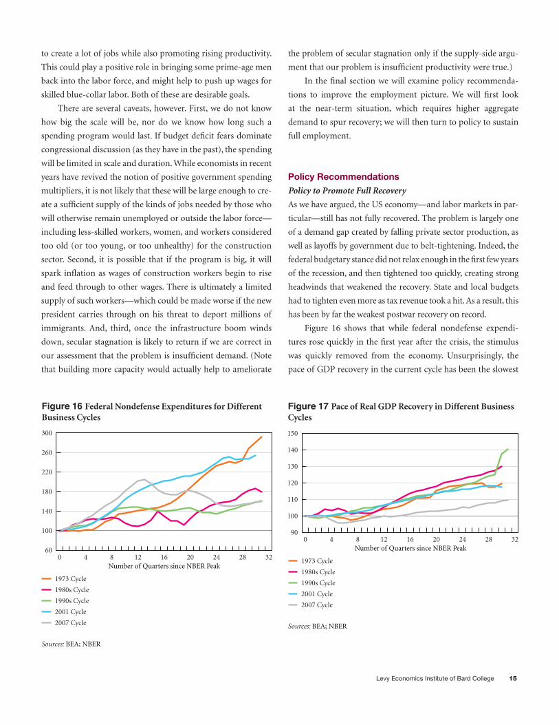
Figure 16 shows that while federal nondefense expendi-

tures rose quickly in the first year after the crisis, the stimulus

was quickly removed from the economy. Unsurprisingly, the

pace of GDP recovery in the current cycle has been the slowest

Sources: BEA; NBER

60

100

140

180

220

260

300

1973 Cycle

1980s Cycle

1990s Cycle

2001 Cycle

2007 Cycle

40

Figure 16 Federal Nondefense Expenditures for DifferentBusiness Cycles

Number of Quarters since NBER Peak128 16 2420 28 32

90

100

110

120

130

140

Figure 17 Pace of Real GDP Recovery in Different BusinessCycles

Sources: BEA; NBER

1973 Cycle

1980s Cycle

1990s Cycle

2001 Cycle

2007 Cycle

40Number of Quarters since NBER Peak

128 16 2420 28

Hand drawn data lines.not quite right compared to excel �les or

Word doc but can’t match because tick marks are absent

32

150


of any cycle in the last 40 years (Figure 17). The real GDP gap is

still sizable, at $250 billion according to real GDP data provided

by the Bureau of Economic Analysis, and according to the latest

real potential GDP data estimated by the Congressional Budget

Office (CBO 2014) (both expressed in 2009 chained dollars).

Since 2007, the CBO has significantly revised down its estimates

for potential GDP, as it lowered its expectations (much as esti-

mates of the NAIRU have traditionally been raised when unem-

ployment outcomes embarrass those making the estimates).

Rather than trying to ramp up federal spending, Congress has

begun to accept lower growth as the new normal. Figure 18

shows that the real GDP gap would currently be at $1.32 tril-

lion if we used the CBO’s 2008 potential GDP estimates (also

expressed in 2009 chained dollars).

By revising its estimate of “potential,” the CBO is willing

to give up nearly $1.3 trillion of output annually. These down-

ward revisions of potential GDP are related to more pessimistic

assumptions of potential employment and investment, as can

be seen in Table 1. In other words, the pessimism is largely due

to the CBO’s expectations of a continuing depression of aggre-

gate demand conditions.

Our calculations show that we are still 20 million jobs short

of being able to declare full employment. It would take, on aver-

age, an increase in payroll employment of 420,000 per month

over the course of the next four years before the economy

would be close to full employment. However, since October

2009, when the unemployment rate peaked at 10 percent, job

creation has averaged around 140,000 jobs per month. The best

year for employment creation since the official end of the reces-

sion was 2014, when job creation averaged around 248,000 jobs

per month. And yet, we have long had persistent calls for Fed

tightening. Until we get to full employment, tightening mon-

etary policy on the basis of the dual mandate is completely

unjustified.

The Way Forward: A Permanent New Deal–style Job

Guarantee

During the stagnation of the Great Depression, Roosevelt’s

New Deal created 13 million jobs in its various direct employ-

ment programs. The biggest program was the Works Progress

Administration, which employed a total of about 8 million

workers—many of them in infrastructure investment of the

type we now sorely need. The creation of a new New Deal pro-

gram could provide the workers we need for many of the infra-

structure projects that Trump and others want, but would go

well beyond this by creating jobs for anyone who is ready and

willing to work. It would be an open-ended job guarantee—not

limited by the labor requirements of any single project—since

it aims to achieve true full employment on a permanent basis.

The federal government would take responsibility to provide

the funding for a base wage to be paid to anyone who works in

the program.20

Table 1 Contributions to the Revision of the CBO’s Projection of Potential Output for 2017 between 2007 and 2014

Decline Contribution to Decline (percentage points) (in percent)

Nonfarm business sector Potential labor hours –2.7 37.7 Capital services –2.4 33.5 Potential total factor productivity –1.4 19.2

Other sectors –0.7 9.6

Total –7.3 100.0

Sources: CBO; authors’ calculations

Figure 18 GDP Gap after the CBO’s Revisions to Potential GDP

Sources: BEA; CBO; authors’ calculations

Trill

ion

s of

US

Dol

lars

10

12

14

16

18

20

Actual Real GDP

Potential GDP Projection, 2008



2015

Q1

2011

Q2

2007

Q3

2000

Q1

2003

Q4

2018

Q4


Roosevelt’s New Deal jobs programs were highly central-

ized, which was appropriate for an economy experiencing a

severe crisis and with large sections of the country underdevel-

oped. If we were to adopt a nationwide job guarantee (paying a

uniform minimum wage) in a new New Deal, however, it would

make sense to decentralize and thereby increase involvement

by state and local government as well as community groups.

Jobs would be directed where they are needed. Projects would

be designed to meet the needs of the community. Proposals

would be submitted by local governments and not-for-profits,

and would go through several layers of approval: local, regional,

state, and federal. Management of the projects would be local,

but evaluated by regional, state, and federal committees.

Wages of program workers would be paid by the federal

government (directly to bank accounts associated with Social

Security numbers), with limited federal funding of additional

project expenses (perhaps limited to 25 percent of the wage bill,

to cover materials and administrative costs). Continued federal

support would depend on evaluation of the success of the proj-

ects. Assessment would include benefits to participants as well

as to the community. In a program of this kind workers would

receive not only income but also a range of other benefits,

including enhanced feelings of self-worth and social inclusion.

Society would benefit from their productive labor and there

would be important macroeconomic effects as well, because

employment in such a program (and hence public spending)

would be strongly countercyclical—helping to stabilize income

and aggregate demand. The labor pool in the program would

also reduce hiring costs for private firms as participants build

a work history.

By targeting those who need jobs, the program would

minimize the inflationary impacts of full employment.21 Unlike

“pump priming”—which does not directly target the unem-

ployed but relies on “trickle-down” and multiplier impacts to

create jobs where they are actually needed—New Deal–style

direct job creation efficiently creates jobs where they are needed.

Further, since the program would pay a uniform base wage, it

would not bid up private sector wages. It would essentially oper-

ate like a floor-price buffer-stock program, much like the agri-

cultural price support programs that also formed part of the

original New Deal program.

The program’s wage (and benefits package) would become

the nation’s minimum wage—preventing other wages from fall-

ing below the floor “price.” If that were initially set above the

prevailing wage, it would lead to a one-time jump, but so long

as it was not increased, the program would dampen wage infla-

tion rather than promote it. This is because the program labor

pool—a “reserve army” of the employed—acts like a buffer

stock of commodities in an agricultural price support program.

When private sector employment and wages begin to climb,

workers are recruited out of the program. Wage increases in the

program become a policy variable and should rise with overall

labor productivity—which will push up private sector wages.

In this manner, the “productivity gap” can be closed directly

through policy.

The program would be phased in as quickly as projects

are approved and begun. Applications by job seekers would be

forwarded to project directors; employment might initially be

assigned by lottery—until a sufficient supply of jobs has been

created. If there are an insufficient number of jobs, the call for

project proposals can be extended to state and federal govern-

ments—until the number of job openings exceeds the number

of job seekers (the measure of full employment indicated by the

20th-century British economist William Beveridge). The pro-

gram would be permanent—through the thick and thin of the

business cycle—hiring more workers in downturns and releas-

ing them to the private sector in expansions. Some projects

would also be more or less permanent, while others would sit

on the shelf awaiting recessions to hire the workers shed by the

private sector. In this manner, program employment as well as

the federal government’s spending on the program would be, as

noted, highly countercyclical.

Note that this job guarantee program tackles both short-

and long-term labor market problems. In a downturn, those

who lose their jobs have the choice of working in the program

rather than becoming unemployed or leaving the labor mar-

ket. By reducing long-term unemployment, the program helps

workers to maintain their skills and attachment to the labor

force. Minsky argued that skills upgrading should be a goal of

all the jobs in the program. The program would take workers “as

they are, where they are,” and improve their employability. No

matter how long workers have been out of the labor force, the

program would offer them an opportunity to work.

While the job guarantee program will not resolve all the

problems that today’s workers face, it would make a major dif-

ference in the lives of those now facing the biggest obstacles to

working. Over time, the program would reduce idleness and

involuntary part-time work, and could be used to gradually


increase wages and benefits at the bottom (as program wages

and benefits rise, private employers would have to increase the

remuneration they provide in order to compete). This would

reduce labor market inequality from the bottom up, as Minsky

recommended—an alternative to the supply-side and demand-

side “trickle-down” policies that have failed us.

Notes

1. The report (CEA 2016) is entitled The Long-Term Decline

in Prime-age Male Labor Force Participation.

2. The unemployment rate in November 2016 was 4.6 percent.

According to the FOMC’s summary of economic projec-

tions published in December 2016, the median longer-run

projection for the unemployment rate was 4.7 percent. The

central tendency was between 4.7 and 5.0 percent, and the

range was 4.5–5.0 percent. See FOMC (2016).

3. The U-6 unemployment rate is calculated as the ratio of

unemployed workers plus employed part time for eco-

nomic reasons plus marginally attached to the labor force,

over the civilian labor force plus the number of marginally

attached workers.

4. Those who want and are available to work, looked for work

in the past year, but did not actively search in the previous

month.

5. See Labor Force Statistics from the Current Population

Survey, table A-38, available at bls.gov.

6. Blau and Khan (2013), for example, point out that in 1990,

the United States had the sixth-highest female labor force

participation among OECD countries, and that by 2010 its

rank had fallen to 17th. According to them, one-third of

this relative decline can be explained by the lack of “fam-

ily friendly” policies, including parental leave and public

expenditures on childcare. Also, see Schulte and Durana

(2016), who show that the average cost of full-time care for

children aged 0–4 is now higher than the average cost of

in-state college tuition.

7. See series ID number LNS15026639 of the Current

Population Survey, available at bls.gov.

8. The Augmented Unemployment rate is the ratio of the

unemployed plus those employed part time for economic

reasons plus those in the labor force who want a job now,

over the civilian labor force plus those not in the labor force

who want a job now.

9. The labor force participation rate (LFPR) is the ratio of

those who are employed or looking for jobs (i.e., those in

the labor force) over the civilian noninstitutional popu-

lation (those 16 years of age or older who are not in the

military). Note that the noninstitutionalized population

excludes those who are incarcerated, most of whom are

of working age. Hence, this lowers the denominator of the

ratio, so that a rising rate of incarceration increases the

LFPR, unless those who become incarcerated have had a

higher-than-average labor force participation rate. That

appears unlikely. On the other hand, upon reentry, they

face a lifetime of stigma and lower job prospects, and a

higher likelihood of dropping out of the labor force, in

which case the overall LFPR would decline. Although data

to test which effect is likely to prevail are not available, the

increasing fraction of the population that has been formally

incarcerated is likely to reinforce the long-term decline in

the LFPR.

10. Historically, the labor force participation rates for the age

groups 20–24 and 25–54 are higher than for other age

groups. If the percentage of the population in prime work-

ing age (who have a significantly higher labor participation

rates) is declining relative to the percentage of the civilian

population older than 55, which is the case in the United

States, we would expect, all else equal, the shift in age

demographics to exert downward pressure on the overall

labor force participation rate, as it has. However, the fact

that the LFPR for the 55-and-older age group has increased

by 24 percent since April 2000 means that it has slowed

down the pace of the fall in the overall LFPR that naturally

results from an aging population. Add to that the fact that

the LFPR has fallen for all other age groups (33 percent for

age group 16–19, 10 percent for age group 20–24, and 5

percent for age group 24–55), we can conclude that aging is

a less important factor in the fall of the LFPR than it other-

wise would be.

11. In the period 2006–15, labor force participation for those

older than 55 increased at an average of 0.27 percentage

points per year over the period, while labor force partici-

pation for the group 25–54 declined at an average of 0.11

percentage points per year.

12. For example, for the time period 2009–11, our estimates

show that 64 percent of the decline in the LFPR was due to

non-age-related demographic factors. Similarly, Shierholz


(2012) finds that more than two-thirds of the decline in

the LFPR in that time period was cyclical; Van Zandweghe

(2012) estimates 58 percent; while the CEA (2014) finds

that half of the decline in the LFPR over the same time

period was cyclical.

13. See Labor Force Statistics of the Current Population Survey,

table A-38, available at bls.gov.

14. Disability is the focus of a common supply-side argument.

See, for example, Fujita (2014) and Eberstadt (2016). Fujita

(2014) makes the argument that disability explained 45

percent of the cumulative decline in participation rates

over the period 2000–11.

15. SSI supports blind, elderly, and disabled individuals with-

out a work history.

16. Along those lines, a disturbing trend is that nearly 31 percent

of the prime-age men not in the labor force self-reported

illegal drug use according to a 2004 survey presented by

Eberstadt (2016, 817). This number is staggering, particu-

larly when compared to only 8 percent for those who are

employed and 22 percent for those who are unemployed.

17. Robert Lucas and Thomas Sargent first explored the link

between inflation expectations and actual inflation in their

formulation of the aggregate supply hypothesis. The idea

was that economic agents are forward-looking when for-

mulating expectations about the future—they make use

of all past and current relevant information to forecast

future economic data. The important point is that agents

can never be systematically wrong—so, on average, their

expectations are always correct. Price stability and mone-

tary policy effectiveness require that the public “play along”

and trust the Fed. Unannounced, unanticipated monetary

shocks will cause the “sacrifice ratio” to be high and adjust-

ments to be costly; they also hurt the feelings of the private

sector, which will turn uncooperative on a game-theory

framework, causing economic instability and monetary

policy ineffectiveness.

18. According to Summers, there has been a reduction in the

demand for loanable funds by corporations due to higher

retained earnings, and lower capital equipment prices, at

the same time the supply of loanable funds has increased

due to the increased rate of saving that results from con-

centration of income and wealth in the hands of the top 1

percent.

19. Our view is in line with Papadimitriou et al. (2014, 2015)

and Papadimitriou, Nikiforos, and Zezza (2016).

20. For more analysis of the job guarantee program, see Minsky

(2013), Tcherneva (2012, 2014), and Wray (1998a, 2012).

21. See Minsky (2013) for a detailed argument that the

employer-of-last-resort program would help to stabilize

inflation. Minsky claimed that while moving to inflation

could cause wages and prices to rise, maintaining full

employment through a job guarantee would not cause

them to continue to rise.

References

Aaronson, S., B. Fallick, A. Figura, J. Pingle, and W.

Wascher. 2006. “The Recent Decline in the Labor Force

Participation Rate and Its Implications for Potential

Labor Supply.” Brookings Institution, Brookings Papers on

Economic Activity (Spring): 69–154.

Bernanke, B. 2015. “Why Are Interest Rates So Low, Part 2:

Secular Stagnation.” Brookings Blog, March 31.

Blau, F., and L. Kahn. 2013. “Female Labor Supply: Why Is the

US Falling Behind?” Discussion Paper No. 7140. Bonn:

Institute for the Study of Labor.

Carnevale, A. P., T. Jayasundera, and A. Gulish. 2015. “Six

Million Missing Jobs: The Lingering Pain of the Great

Recession.” Washington, D.C.: The Georgetown University

Center on Education and the Workforce.

CEA (Council of Economic Advisers). 2014. The Labor

Force Participation Rate Since 2007: Causes and Policy

Implications. Report of the Executive Office of the

President of the United States. Washington, D.C.:

Government Printing Office. July. Available at: obam-

awhitehouse.archives.gov/sites/default/files/docs/labor_

force_participation_report.pdf.

———. 2016. The Long-Term Decline in Prime-age Male

Labor Force Participation. Report of the Executive Office

of the President of the United States. Washington,

D.C.: Government Printing Office. June. Available at:

obamawhitehouse.archives.gov/sites/default/files/page/

files/20160620_primeage_male_lfp_cea.pdf.

CBO (Congressional Budget Office). 2014. Revisions to CBO’s

Projection of Potential Output since 2007. Washington,

D.C.: CBO. February 28.


Eberstadt, N. 2016. Men without Work: America’s Invisible

Crisis. West Conshohocken: Templeton Press. Kindle

Edition.

Fleck, S., J. Glaser, and S. Sprague. 2011. “The Compensation–

Productivity Gap: A Visual Essay.” Bureau of Labor

Statistics, Monthly Labor Review (January).

FOMC (Federal Open Market Committee). 1996. “Meeting

of the Federal Open Market Committee, September 24,

1996.” Transcript.

———. 2016. “Minutes of the Federal Open Market

Committee, December 13–14, 2016: Summary of

Economic Projections.”

Fujita, S. 2014. On the Causes of Declines in the Labor Force

Participation Rate. Research Rap Special Report. Federal

Reserve Bank of Philadelphia. February 6.

Minsky, H. P. 2013. Ending Poverty: Jobs, Not Welfare.

Annandale-on-Hudson: Levy Economics Institute of Bard

College.

Mitchell, B. 2014. “Decomposing the Decline in the US

Participation Rate for Ageing.” Billy Blog, July 22.

Papadimitriou, D. B., G. Hannsgen, M. Nikiforos, and G.

Zezza. 2015. Fiscal Austerity, Dollar Appreciation, and

Maldistribution Will Derail the US Economy. Strategic

Analysis. Annandale-on-Hudson: Levy Economics

Institute of Bard College. May.

Papadimitriou, D. B., M. Nikiforos, and G. Zezza. 2016.

Destabilizing an Unstable Economy. Strategic Analysis.


College. March.

Papadimitriou, D. B., M. Nikiforos, G. Zezza, and G. Hannsgen.

2014. Is Rising Inequality a Hindrance to the US Economic

Recovery? Strategic Analysis. Annandale-on-Hudson: Levy

Economics Institute of Bard College. April.

Pigeon, M. A., and L. R. Wray. 1999a. “Demand Constraints

and Economic Growth.” Working Paper No. 269.


College. May.

———. 1999b. Down and Out in the United States: An Inside

Look at the Out of Labor Force Population. Public Policy

Brief Highlights No. 54. Annandale-on-Hudson: Levy

Economics Institute of Bard College. July.

Schulte, B., and A. Durana. 2016. The Care Report. Washington,

D.C.: New America.

Sen, A. K. 1999. Development as Freedom. Oxford: Oxford

University Press.

Summers, L. 2014. “U.S. Economic Prospects: Secular

Stagnation, Hysteresis, and the Zero Lower Bound.”

Business Economics 49(2): 65–73.

———. 2016. “Men Not at Work.” Financial Times,

September 23.

Tcherneva, P. 2012. Full Employment through Social

Entrepreneurship: The Nonprofit Model for Implementing

a Job Guarantee. Policy Note 2012/2. Annandale-on-

Hudson: Levy Economics Institute of Bard College. March.

———. 2014. “Full Employment: The Road Not Taken.”

Working Paper No. 789. Annandale-on-Hudson: Levy

Economics Institute of Bard College. March.

Van Zandweghe, W. 2012. “Interpreting the Recent Decline

in Labor Force Participation.” Federal Reserve Bank of

Kansas City, Economic Review (First Quarter): 5–34.

Williams, J. 2016. “After the First Rate Hike.” Presentation to the

California Bankers Association, Santa Barbara, January 8.

Wray, L. R. 1998a. Understanding Modern Money: The Key

to Full Employment and Price Stability. Northampton:

Edward Elgar.

———. 1998b. Did the Clinton Rising Tide Raise All Boats?

Job Opportunity for the Less Skilled. Public Policy Brief

Highlights No. 45A. Annandale-on-Hudson: Levy

Economics Institute of Bard College. October.

———. 2004. The Fed and the New Monetary Consensus: The

Case for Rate Hikes, Part Two. Public Policy Brief No. 80.


College. December.

———. 2007. “Demand Constraints and Big Government.”

Working Paper No. 488. Annandale-on-Hudson: Levy

Economics Institute of Bard College. January.

———. 2012. Modern Money Theory: A Primer on

Macroeconomics for Sovereign Monetary Systems. New

York: Palgrave Macmillan.

Yellen, J. 2015. “Inflation Dynamics and Monetary Policy.”

Philip Gamble Memorial Lecture, University of

Massachusetts Amherst, September 24.


About the Authors

flavia dantas is assistant professor of economics at the State University of New York at Cortland,

where she teaches classes in mathematical economics, public policy, macroeconomics, and mon-

etary theory and policy. Her current research focuses on different aspects of domestic and interna-

tional liquidity creation and their implication for monetary policy and financial stability. She also

conducts research in the fields of full employment policy, and modern money theory and fiscal

policy. Dantas received her Ph.D. from the University of Missouri–Kansas City in 2013.

Senior Scholar l. randall wray is a professor of economics at Bard College. His current research

focuses on providing a critique of orthodox monetary theory and policy, and the development

of an alternative approach. He also publishes extensively in the areas of full employment pol-

icy and, more generally, fiscal policy. With President Dimitri B. Papadimitriou, he is working to

publish, or republish, the work of the late financial economist Hyman P. Minsky, and is using

Minsky’s approach to analyze the current global financial crisis. Wray’s most recent book is Why

Minsky Matters: An Introduction to the Work of a Maverick Economist (Princeton University Press,

2016). He is also the author of Money and Credit in Capitalist Economies: The Endogenous Money

Approach (Edward Elgar, 1990), Understanding Modern Money: The Key to Full Employment and

Price Stability (Edward Elgar, 1998), The Rise and Fall of Money Manager Capitalism: Minsky’s

Half Century from World War Two to the Great Recession (with É. Tymoigne; Routledge, 2013),

and Modern Money Theory: A Primer on Macroeconomics for Sovereign Monetary Systems (Palgrave

Macmillan, 2012; 2nd rev. ed., 2015). He is coeditor of, and a contributor to, Money, Financial

Instability, and Stabilization Policy (Edward Elgar, 2006) and Keynes for the 21st Century: The

Continuing Relevance of The General Theory (Palgrave Macmillan, 2008). Wray taught at the

University of Denver from 1987 to 1999 and at the University of Missouri–Kansas City from 1999

to 2016, and has been a visiting professor at the Universities of Paris and Rome (La Sapienza). He

holds a BA from the University of the Pacific and an MA and a Ph.D. from Washington University,

where he was a student of Minsky.

FULL EMPLOYMENT: ARE WE THERE YET? - Levy ... Bard College Levy Economics Institute Levy Economics...

Documents

Transcript of FULL EMPLOYMENT: ARE WE THERE YET? - Levy ... Bard College Levy Economics Institute Levy Economics...