FULL AC NETWORK INTEGRATED CORE SOLVER : SUPEROPF ...

FULL AC NETWORK INTEGRATED CORE SOLVER : SUPEROPF FRAMEWORK

Hsiao-Dong Chiang, Bin Wang and Patrick Causgrove

Bigwood Systems, Inc.

Ithaca, New York

Bigwood Systems Inc., 2012 2

Issues with Current Generation of Optimal Power Flow

• Current solvers are still not sufficiently robust • Current solvers still can not correctly handle

stability constraints • Optimal power flow solution is NOT a global

optimal solution • Solvers only compute one (local) optimal

solution while there are multiple local optimal solutions

• Each OPF solution corresponds to one location marginal pricing (which OPF solution is the right one ?)

Phase I: Robust AC OPF Solvers

1.(support industrial model) A commercial-grade core SuperOPF software supporting various industrial-grade power system models such as

(i) CIM-compliance; and (ii) PSS/E data format 2. A multi-stage OPF solver with adaptive homotopy-based Interior Point Method for large-scale power systems (14,000-bus data)


Adaptive Homotopy-guided, Active-Set-Assisted Primal-Dual Interior Point OPF

Solver (Patent pending, 2014) 1. Homotopy-based Methodology (continuation

method + adaptive step-size) 2. Domain-knowledge-based 3. Active-set assisted 4. IPM method (core solver)

• 118-bus system

• 3120-bus system

SuperOPF, PSSE & MATPOWER tests results (2014)

Solver MIPS FMINCON KNITRO IPOPT Success Rate 69/101 101/101 101/101 101/101

Solver TRANLM PSSE SuperOPF Success Rate 101/101 1001/1001 1001/1001

Solver MIPS FMINCON KNITRO IPOPT Success Rate 1/101 1/101 36/101 1/101

Solver TRANLM PSSE SuperOPF Success Rate 1/101 0/1001 1001/1001


Results: Efficiency and Robustness (Analytical Jacobian matrices)

Loading Condition

One-Staged Scheme

Multi-Staged Scheme

1 Succeeded Succeeded 2 Succeeded Succeeded 3 Succeeded Succeeded 4 Succeeded Succeeded 5 Failed Succeeded 6 Failed Succeeded 7 Failed Succeeded 8 Failed Succeeded 9 Failed Succeeded

10 Failed Succeeded

Base case

Without constraint analysis • Converged in 217 iterations • CPU time: 177 seconds • OPF loss: 3251.284MW

With constraint analysis • Converged in 191 iterations • CPU time: 143 seconds • OPF loss: 3251.353MW

Effects of constraint analysis Robustness of our method

Stage I: OPF Constraint Analyzer

Stage II: Simple OPF w/o

Thermal Limits

Stage III: Homotopy OPF w/ Active Thermal Limits

Stage IV: Sensitivity Analyzer

for Discretization

Input Data OPF Result

OPF without thermal constraints OPF with active thermal constraints

Sensitivity based adjustment

Super-OPF (continuous and discrete variables)

Super-OPF Method

Super-OPF Dimensions

Stage I: OPF Constraint Analyzer

Stage II: Simple OPF w/o

Thermal Limits

Stage III: Homotopy OPF w/ Active Thermal Limits

Stage IV: Sensitivity Analyzer

for Discretization

Input Data OPF Result

System: Buses: 13183 Loads: 9691 Generators: 2304 Branches: 18168 Transformers: 1410 Switched shunts: 1404

OPF Dimensions: Dimension of x: 31134 Nonlinear equality constraints: 26366 Nonlinear inequality constraints: 0 Total equality constraints: 26367 Total inequality constraints: 35902

OPF Dimensions: Dimension of x: 31134 Nonlinear equality constraints: 26366 Nonlinear inequality constraints: varying (<100) Total equality constraints: 26367 Total inequality constraints: >35902 (varying)

System: Continuous variables: 28320 Discrete variables: 2814

13183-Bus System

2014/8/7

Challenges: Problem Formulations and Solvers

min ( )C x

Subject to: ( ) 0( ) 0

h xg x

=≤

( ) 0h x =

x x x≤ ≤

However, security-constrained OPF can not be expressed as the above analytical form: i. Power balance equations:

ii. Voltage limit constraints:

iii. Thermal limit constraints:

iv. Transient-stability constraints:

v. Voltage stability constraints:

( ) 0g x ≤

???

???

2014/8/7

Implications: (i) It is not possible to represent

them in explcit forms. (ii) approximations are subject

to incorrect stability assessment. ( ) 0( ) 0

h xg x

=≤

i. Transient-stability constraints:

ii. Voltage stability constraints:

Stability Constraints Can not be explicitly dealt with

Making several recently proposed methods not applicable, such as • J.Lavaei and S.Low, “Zero Duality Gap in Optimal Power Flow

Problem,” IEEE Transactions on Power Systems, vol.27, no.1, pp. 92–107, February 2012.

• D.K. Molzahn, J.T. Holzer, and B.C. Lesieutre, and C.L. DeMarco, “Implementation of a Large-Scale Optimal Power Flow Solver Based on Semidefinite Programming,” IEEE Transactions on Power Systems, vol. 28, no. 4, pp. 3987-3998, November 2013.


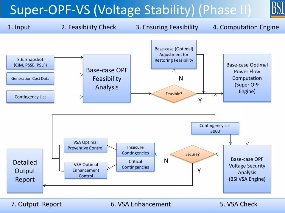
Super-OPF-VS (Voltage Stability) (Phase II)

Base-case Simulation

Generation Cost Data

S.E. Snapshot (CIM, PSSE, PSLF)

Contingency List Feasible?

Base-case Optimal Power Flow

Computation (Super OPF

Engine)

Y

Base-case (Optimal) Adjustment for

Restoring Feasibility

N Base-case OPF

Feasibility Analysis

Base-case OPF Voltage Security

Analysis (BSI VSA Engine)

Secure? Insecure

Contingencies

Critical Contingencies

N

VSA Optimal Preventive Control

VSA Optimal Enhancement

Control

Detailed Output Report

Y

Contingency List 3000

1. Input 2. Feasibility Check 3. Ensuring Feasibility 4. Computation Engine

7. Output Report 6. VSA Enhancement 5. VSA Check

Feedback Comments

• “explicitly include voltage stability constraints

which would allow the solutions to more fully utilize existing capacity throughout electric power networks. This feature alone could be extremely valuable. “

NSA (Newton Power Flow)

ILCT

MILP (Unit Commitment)

BSI VSA (to generate on-line

VS constraint)

Replaced by

Off-line study to generate voltage stability (VS) constraints (updated infrequently)

AC Power flow

NYISO

Super-OPF Contingency Analysis

BSI VSA Preventive Control

Initial Power Flow from State Estimator

Super-OPF Solution

1062 N-1 Contingencies

A practical 6534-Bus System

0 0 3010.028 -20.088 0 3010.028 1 21 -0.305 -0.305 3 0.000 2 34 -0.218 -0.218 6 0.000 3 691 -0.100 -0.100 17 0.000 4 8 -0.066 -0.066 1 0.000 5 35 -0.060 -0.060 5 0.000 6 24 -0.056 -0.056 2 0.000 7 36 -0.015 -0.015 4 0.000 8 639 1353.153 -9.031 12 2347.311 9 281 1884.894 -12.579 10 1397.252 10 282 1884.894 -12.579 11 1397.252 11 491 2715.639 -18.123 14 2481.276 12 492 2715.639 -18.123 13 2481.276 13 561 2716.463 -18.129 15 2485.825 14 521 2730.695 -18.224 16 2503.604 15 572 2789.834 -18.619 41 2789.834 16 864 2791.814 -18.632 42 2791.814 17 863 2791.814 -18.632 43 2791.814 18 628 2805.778 -18.725 44 2805.778 19 690 2807.721 -18.738 18 2619.026 20 684 2822.604 -18.837 47 2822.604

Load margin: 3010MW Objective (loss): 2793.6MW 7 insecure contingencies

0 0 4840.000 -32.301 0 4840.000 1 21 -0.285 -0.285 3 0.000 2 34 -0.253 -0.253 5 0.000 3 35 -0.071 -0.071 4 0.000 4 8 -0.050 -0.050 1 0.000 5 24 -0.042 -0.042 2 0.000 6 561 4373.778 -29.189 16 4304.356 7 491 4386.839 -29.276 15 4284.000 8 492 4386.839 -29.276 14 4284.000 9 691 4404.315 -29.393 20 4404.315 10 521 4407.446 -29.414 17 4316.588 11 690 4437.187 -29.612 23 4437.187 12 281 4494.606 -29.996 18 4381.087 13 282 4494.606 -29.996 19 4381.087 14 639 4508.597 -30.089 21 4413.366 15 428 4544.092 -30.326 25 4483.436 16 432 4544.092 -30.326 26 4483.436 17 431 4544.092 -30.326 27 4483.436 18 430 4544.092 -30.326 28 4483.436 19 429 4544.092 -30.326 29 4483.436 20 501 4555.107 -30.399 30 4511.405

Load margin: 4840MW Objective (loss): 1642.8MW 5 insecure contingencies

0 0 4840.161 -32.302 0 4840.161 1 561 4376.021 -29.204 23 4303.308 2 492 4389.094 -29.291 22 4282.792 3 491 4389.094 -29.291 21 4282.792 4 521 4409.681 -29.429 24 4315.462 5 690 4436.558 -29.608 25 4436.558 6 691 4509.283 -30.094 6 2244.418 7 431 4546.083 -30.339 26 4482.817 8 430 4546.083 -30.339 27 4482.817 9 429 4546.083 -30.339 28 4482.817 10 428 4546.083 -30.339 29 4482.817 11 432 4546.083 -30.339 30 4482.817 12 501 4556.994 -30.412 31 4510.822 13 509 4564.158 -30.460 32 4514.185 14 281 4571.971 -30.512 14 2416.908 15 282 4571.971 -30.512 15 2416.908 16 506 4577.873 -30.551 33 4534.745 17 662 4580.186 -30.567 38 4550.269 18 663 4580.186 -30.567 39 4550.269 19 456 4585.097 -30.599 34 4536.546 20 455 4585.097 -30.599 35 4536.546

Load margin: 4840MW Objective (loss): 1674.6MW No insecure contingency

Phase III was focused on the following enhancements

(i) deal with multiple base-cases (i.e., co-optimize multiple base-cases)

(iii) deal with uncertainties of wind generations and other renewables

Topicss Enhancements

Co-optimization over multiple scenario(functions)

(ii) deal with thermal limits and voltage limits under AC power flow models of a large set of contingencies.

Commercial-grade packages (applications)

Renewables (uncertainties)

This phase is focused on the following enhancements

(vii) Engage utility companies to provide their assessment of and interest in adopting SuperOPF.

(viiii) Co-optimized SuperOPF- Static + renewables + contingency package

Topics Enhancements

Co-optimization over multiple scenario(functions)

(viii) Engage utility companies to assist the development of SuperOPF.

Commercial-grade packages (applications)

Uncertainties in contingencies

• Objective: minimizing the expected cost across all the scenarios

𝑚𝑚𝑖𝑖𝑖𝑖

𝑠𝑠. 𝑡𝑡.

𝑓𝑓 𝑥𝑥 = 𝑓𝑓0 𝑥𝑥0 + �𝑝𝑝𝑘𝑘[𝑓𝑓𝑘𝑘 𝑥𝑥𝑘𝑘 + 𝑐𝑐𝑘𝑘 𝑥𝑥𝑘𝑘 − 𝑥𝑥0 ]𝐾𝐾

𝑘𝑘=1ℎ0 𝑥𝑥 = 0𝑔𝑔0 𝑥𝑥 ≤ 0… …ℎ𝐾𝐾 𝑥𝑥 = 0𝑔𝑔𝐾𝐾 𝑥𝑥 ≤ 0

𝑓𝑓0 𝑥𝑥0 : base case cost

𝑐𝑐𝑘𝑘 𝑥𝑥𝑘𝑘 − 𝑥𝑥0 : cost of scenario-induced deviations (from base-case)

𝑝𝑝𝑘𝑘: probability for k-th scenario

𝑓𝑓𝑘𝑘 𝑥𝑥𝑘𝑘 : k-th base cost (reserves, load shedding, etc)

SuperOPF Co-optimization

𝑥𝑥 = 𝑥𝑥0, 𝑥𝑥1,⋯ , 𝑥𝑥𝐾𝐾 : optimization variables

𝑥𝑥𝑖𝑖 = (Θ𝑘𝑘 ,𝑉𝑉𝑘𝑘 ,𝑇𝑇𝑘𝑘 , 𝑆𝑆𝑘𝑘 ,𝐵𝐵𝑘𝑘 ,𝑃𝑃𝐺𝐺𝑘𝑘 ,𝑄𝑄𝐺𝐺𝑘𝑘): variables of the k-th scenario (0: base case)


Type-2 scenario: Base case + contingency 𝑚𝑚𝑖𝑖𝑖𝑖 𝑓𝑓(𝑥𝑥)𝑠𝑠. 𝑡𝑡. 𝑃𝑃𝑖𝑖 𝑥𝑥 + 𝑃𝑃𝐷𝐷𝑖𝑖 − 𝑃𝑃𝐺𝐺𝑖𝑖 = 0 1 ≤ 𝑖𝑖 ≤ 𝑖𝑖𝐵𝐵

𝑄𝑄𝑖𝑖 𝑥𝑥 + 𝑄𝑄𝐷𝐷𝑖𝑖 − 𝑄𝑄𝐺𝐺𝑖𝑖 = 0

𝑆𝑆𝑘𝑘 = 𝑃𝑃𝑖𝑖𝑖𝑖2 𝑥𝑥 + 𝑄𝑄𝑖𝑖𝑖𝑖2 (𝑥𝑥) ≤ 𝑆𝑆𝑘𝑘𝑚𝑚𝑚𝑚𝑚𝑚

𝑥𝑥𝑚𝑚𝑖𝑖𝑚𝑚 ≤ 𝑥𝑥 ≤ 𝑥𝑥𝑚𝑚𝑚𝑚𝑚𝑚𝑖𝑖, 𝑗𝑗 ∈ 𝐿𝐿�

𝐿𝐿�: L excludes contingent branches

Type 4 scenario: Base case + renewable energy + contingency

𝑚𝑚𝑖𝑖𝑖𝑖 𝑓𝑓(𝑥𝑥)𝑠𝑠. 𝑡𝑡. 𝑃𝑃𝑖𝑖 𝑥𝑥 + 𝑃𝑃�𝐷𝐷𝑖𝑖 − 𝑃𝑃𝐺𝐺𝑖𝑖 = 0 1 ≤ 𝑖𝑖 ≤ 𝑖𝑖𝐵𝐵

𝑄𝑄𝑖𝑖 𝑥𝑥 + 𝑄𝑄�𝐷𝐷𝑖𝑖 − 𝑄𝑄𝐺𝐺𝑖𝑖 = 0


𝑥𝑥𝑚𝑚𝑖𝑖𝑚𝑚 ≤ 𝑥𝑥 ≤ 𝑥𝑥𝑚𝑚𝑚𝑚𝑚𝑚

𝑖𝑖, 𝑗𝑗 ∈ 𝐿𝐿�

Type-1 scenario: Base case 𝑚𝑚𝑖𝑖𝑖𝑖 𝑓𝑓(𝑥𝑥)

𝑠𝑠. 𝑡𝑡. 𝑃𝑃𝑖𝑖 𝑥𝑥 + 𝑃𝑃𝐷𝐷𝑖𝑖 − 𝑃𝑃𝐺𝐺𝑖𝑖 = 0 1 ≤ 𝑖𝑖 ≤ 𝑖𝑖𝐵𝐵𝑄𝑄𝑖𝑖 𝑥𝑥 + 𝑄𝑄𝐷𝐷𝑖𝑖 − 𝑄𝑄𝐺𝐺𝑖𝑖 = 0


𝑥𝑥𝑚𝑚𝑖𝑖𝑚𝑚 ≤ 𝑥𝑥 ≤ 𝑥𝑥𝑚𝑚𝑚𝑚𝑚𝑚𝑖𝑖, 𝑗𝑗 ∈ 𝐿𝐿

𝑖𝑖𝐵𝐵: the number of buses 𝐿𝐿: the set of branches Type 3 scenario: Base case + renewable energy 𝑚𝑚𝑖𝑖𝑖𝑖 𝑓𝑓(𝑥𝑥)𝑠𝑠. 𝑡𝑡. 𝑃𝑃𝑖𝑖 𝑥𝑥 + 𝑃𝑃�𝐷𝐷𝑖𝑖 − 𝑃𝑃𝐺𝐺𝑖𝑖 = 0 1 ≤ 𝑖𝑖 ≤ 𝑖𝑖𝐵𝐵

𝑄𝑄𝑖𝑖 𝑥𝑥 + 𝑄𝑄�𝐷𝐷𝑖𝑖 − 𝑄𝑄𝐺𝐺𝑖𝑖 = 0


𝑥𝑥𝑚𝑚𝑖𝑖𝑚𝑚 ≤ 𝑥𝑥 ≤ 𝑥𝑥𝑚𝑚𝑚𝑚𝑚𝑚

𝑖𝑖, 𝑗𝑗 ∈ 𝐿𝐿

𝑃𝑃�𝐷𝐷,𝑄𝑄�𝐷𝐷: equivalent loads with renewable energies

Four types of scenarios

Internal Models

Input Scenarios

Base-case Data

Contingency List

Renewable Forecasts

Master NLP

Sub NLP #1

Sub NLP #2 SuperOPF

Cooptimization Solver

Base-case Contingent scenario Renewable scenario

Problem Constructor

A tree-like structure

Sub NLP #N

……


Contingent + renewable scenario

Base Case

Contingencies +

Renewable Energy Forecasts

Internal Combinatorial

Scenarios K=(M+1)*(N+1)


𝑚𝑚𝑖𝑖𝑖𝑖

𝑠𝑠. 𝑡𝑡.

𝑓𝑓 𝑥𝑥 = 𝑓𝑓0 𝑥𝑥0 + �𝑝𝑝𝑘𝑘[𝑓𝑓𝑘𝑘 𝑥𝑥𝑘𝑘 + 𝑐𝑐𝑘𝑘 𝑥𝑥𝑘𝑘 − 𝑥𝑥0 ]𝐾𝐾

𝑘𝑘=1ℎ0 𝑥𝑥 = 0𝑔𝑔0 𝑥𝑥 ≤ 0… …ℎ𝐾𝐾 𝑥𝑥 = 0𝑔𝑔𝐾𝐾 𝑥𝑥 ≤ 0


𝑚𝑚𝑖𝑖𝑖𝑖𝑠𝑠. 𝑡𝑡

𝑓𝑓0 𝑃𝑃0ℎ0 𝑥𝑥 = 0𝑔𝑔0 𝑥𝑥 ≤ 0

M: # of

contingencies N: # of

renewable energy forecasts

Phase 1

Solve the type-1 base case OPF

Multi-phase Approach

Phase 2

Solve M type-2 and N type-

3 scenario OPFs

Phase 3

Solve M×N type-4 scenario OPFs

Phase 4

Solve the whole co-optimization OPF

• A multi-phase scheme is developed in which base case OPF solutions are used as initial points for solving scenario problems. A combination of all sub-problem solutions is used as the initial point for the entire co-optimization problem.

Base-case scenario Contingent scenario Renewable scenario Contingent + renewable scenario

• Two practical large-scale systems • a 6534-bus system • A 13183-bus system

• Simulation environment: • 2.6GHz quad-core Intel i7-3720QM processor

(Turbo boost to 3.6GHz), 16GB 1600MHz DDR3 RAM, Mac OSX 10.8.4, GCC 4.8.1

Numerical Simulations

Base Case

Contingencies +

Renewable Energy Forecasts

Internal Combinatorial

Scenarios SuperOPF Co-optimization

Co-optimization Results on a 6500-bus System

# of internal scenarios: 15

# of contingencies: 2 # of renewable

forecasts: 4 • # of optimization variables:

226,215; • # of constraints: 287,360

(equality: 181,260; inequality: 106,100);

• # of Hessian non-zeros: 3 190 566

System: Buses: 6534 Loads: 2901 Generators: 1903 Branches: 8295 Transformers: 294 Switchable shunts: 520

Sub-problem Scenario p F(x) # of

Iters CPU Time

(sec) Sub-

problem Scenario p F(x) # of Iters

CPU Time (sec)

Initial PF 80.418985 9 Base case +

Renewable 2 + Contingency 2

0.573% 21.076384 79 10.38

1 Base case 21.085284 80 10.48 10 Base case + Renewable 3 1.28% 21.089217 77 10.11

2 Base case + Contingency 1 10% 21.106819 79 10.52 11

Base case + Renewable 3 + Contingency 1

0.128% 21.110689 74 9.70

3 Base case + Contingency 2 10% 21.085464 78 10.32 12


0.128% 21.089421 77 10.09

4 Base case + Renewable 1 3.04% 21.172620 79 10.46 13 Base case +

Renewable 4 5.60% 21.218402 75 9.88

5 Base case +


0.304% 21.194469 80 10.43 14


0.560% 21.240219 78 10.31

6 Base case +


0.304% 21.173087 80 10.58 15


0.560% 21.218608 76 10.26

7 Base case + Renewable 2 5.73% 21. 076129 83 10.92

Cooptimization problem 21.129602 310 2281.02 (i.e. 38 min.

8 Base case +


0.573% 21. 097419 82 10.85

Co-optimization Results on CAISO System

Proposed Requirements for Scenario Reduction Schemes

(speed and robust measure) It should be fast and robust to operating conditions

(efficiency measure) the retain important information with the least number of scenarios.

(reliability measure) identify all representative scenarios that properly maintain important information of stochastic variables.

Scenario Reduction Techniques

• Forward selection and backward reduction are the most used scenario reduction technique. • These methods all focus on : “distance” between the selected scenario set and the original scenario set. They are problem-independent.

Our Proposed Scenario Reduction Scheme for Voltage Stability

• Problem-dependent

Stage II: Screening and Ranking Scheme (effect, output space)

Stage I: Cluster Scheme (input space)

Stage III: Detailed Analysis (effect, output space)

Voltage Stability Analysis Under a large number of scenarios

Application-Oriented Scheme

Voltage Stability Analysis Under Uncertainty (Cluster + Screening + ranking + detailed analysis)

In comparison with Monte Carlo method (Scenario : 5000)

IEEE 118-bus Test System

(Renewables at 1, 7, 40, 78, 117) Weibull distribution

Reduction Ratio Accuracy(%) Missing

Scenarios

99.08% 100% 0

Scenarios 5000

Stage I & II Reduce to 46 scenarios

Stage III Reduce to 17 scenarios

Voltage Stability Analysis Under Uncertainty (Cluster + Screening + ranking + detailed analysis)

Poland 3120-bus

(23, 68, 69, 70, 261, 263, 1393, 1395, 1398, 3100, 3101, and 3102)

Weibull distribution

Reduction Ratio Accuracy(%)

Critical Missing

Scenarios

98.52% 100% 0

Scenarios 5000

Stage I & II Reduce to 74 scenarios

Stage III Reduce to 29 scenarios

Scenario Reduction Scheme for OPF (a challenging one)

• Problem-dependent

Stage II: Screening and Ranking Scheme (effect, output space)

Stage I: Cluster Scheme (input space)

Stage III: Detailed Analysis (effect, output space)

Under a large number of scenarios

Application-Oriented Scheme

CO

NC

LUSI

ON

SuperOPF is an advanced & comprehensive ACOPF solver needed by modern power systems.

Innovation prevails!

Commercialization of the SuperOPF Framework:

Comments on SuperOPF from Targeted Early Adopters in the Electric Utility Industry


Industry Participation Component of Phase 3 Work

• Convince ISOs, Balancing Authorities and Transmission Owners that the way to characterize operational risk is to move to the SuperOPF stochastic co-optimize

Objective

Convince RTOs/ISOs, Reliability Coordinators, Balancing Authorities and Transmission Owners that the way to characterize operational risk is to move to the SuperOPF stochastic co-optimization formulation

1. • Identify Industry partner

organizations and key individuals in each that will support this technology transition and the role they are willing to play

2. • Identify applications,

functionality, hurdles to overcome and the best path forward.


TVA Contacts

Josh Shultz Operations

Tom Cain Planning

Key Contacts


TVA Observations

Planning

General

Operations

Static stability constraints with contingency Setting voltage schedules Minimizing number of controls for

reliability Co-optimizing transfer capability and

generation dispatch to provide proven cost-benefit

Help limit exposure to weak adjoining networks (500kv/161kv transition)

Currently in discussions with TVA, regarding Voltage Scheduling Study using SuperOPF

Help addressing NERC requirements

Dynamic stability constraints with contingency

Co-optimization of MW and MVAR is a unique and valuable capability

Scenario co-optimization Peak Load Reduction


PJM Contacts

Jianzhong Tong Operations

Biagio Pinto Outage Analysis Technology

Jeremy Lin Interregional Planning

Byoungkon Choi Transmission Planning

Key Contacts


PJM Observations

• Look-ahead (short–term up to 4 hours) for renewables using co-optimization

• Application to the day-ahead to address renewable intermittency and pre-planning of reserve generation

Power Market & Operations

• Static & Dynamic stability constraints with contingency

Operations & Planning


ISO-NE Contacts

Eugene Litvinov Director-Business Architecture and Technology

Xiaochuan Luo

Tongxin Zheng

Key Contacts


ISO-NE Observations

Operations

General

Power Market

Control actions should be accounted for in the optimization

Setting transfer limits based on margins to limits (thermal, voltage, stability)

Cost of operating the market under SuperOPF must be considered and compared to DC-OPF

This SuperOPF AC formulation is the most accurate

Operation of the system with huge margins may change in future; there is opportunity for Super OPF, if results are high quality, accurate, and the solver is robust

A proven SuperOPF would serve as an industry benchmark for markets

ISO-NE would like to see a study done to assess SuperOPF the impact on the operation of the market

ISO-NE is currently co-funding a study with BSI to compare SuperOPF to ISO-NE Production Software


CAISO Contacts

Mark Rothleder Vice President of Market Quality and Renewable Integration

Khaled Abdul-Rahman Director, Power Systems and Smart Grid Technology Development

Key Contacts


CAISO Observations OPERATIONS

POWER MARKET & OPERATIONS

PLANNING & OPERATIONS

GENERAL

Non-linear OPF needed for the CAISO power market

SuperOPF with handling voltage stability as a constraint is of value to the power market

Ramp Constraints in model Co-optimization of worst scenarios

especially with renewables, Inclusion of AGC response into

SuperOPF to deal with renewable integration

Require good real-time performance

State Estimation Improvements

Static & Dynamic stability constraints with contingency

Operational Reserve requirements with renewables

Innovation prevails!

2014 Project Title: Study of Co-optimization Stochastic

SuperOPF Applications in the CAISO System

Theme: Co-optimization Stochastic SuperOPF-renewables


Project Overview

Study the impact of co-optimization in improving key challenges in the CAISO system using the commercial-grade SuperOPF tool

CAISO is our partner for the project offering in-kind services including: Technical expertise Data analysis Testing Results review Evaluations of the work and overall concepts


Study at CAISO: Primary Objectives

Co-optimize the objective function and the updated worst scenario for voltage stability

Co-optimize the objective function, operational reserve and renewable energy. In addition, the ramp rate of renewable energy should be included


Study at CAISO: Secondary Objectives

Handle the ramp constraints of generation

Handle constraints needed for LMP calculations and required outputs for the power market


Project Deliverables

Demonstration using CAISO data – SuperOPF software which can co-optimize the objective function and the updated worst scenario for voltage stability

Demonstration using CAISO data – SuperOPF software which can co-optimize the objective function, operational reserve and the renewable energies with the inclusion the ramp rate of renewable energy.

Demonstration using CAISO data – SuperOPF software equipped with the ramp constraints of generations

Demonstration using CAISO data – Super-OPF software which can handle constraints needed for LMP calculations and outputs required for the power market


Project Deliverables (2)

Regular meetings with CAISO (including 2 face-to-face meetings)

Quarterly Progress Reports Compiled reports of CAISO feedback Users’ manual for the commercial-grade

Co-optimization SuperOPF software. Design manual for the commercial-grade

Co-optimization SuperOPF software Project final report


Thank you

FULL AC NETWORK INTEGRATED CORE SOLVER : SUPEROPF ...

Documents

Transcript of FULL AC NETWORK INTEGRATED CORE SOLVER : SUPEROPF ...