Fuel Economy and Annual Travel for Passenger Cars and ...
253
US. Department of Transportation National Highway Traffic Safety Administration DOT HS 806 971 May 1986 NHTSA Technical Report Fuel Economy and Annual Travel for Passenger Cars and Light Trucks: National On-Road Survey This document is available to the public from the National Technical Information Service, Springfield, Virginia 22161.
Transcript of Fuel Economy and Annual Travel for Passenger Cars and ...

US. Departmentof Transportation
National HighwayTraffic SafetyAdministration
DOT HS 806 971 May 1986
NHTSA Technical Report
Fuel Economy and Annual Travelfor Passenger Cars and Light Trucks:National On-Road Survey
This document is available to the public from the National Technical Information Service, Springfield, Virginia 22161.
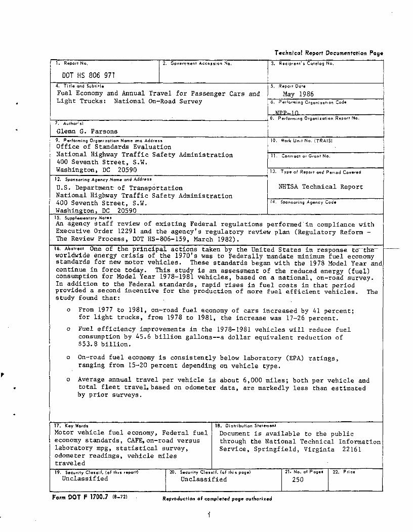
Technical Report Documentation Page
1. Report No.
DOT HS 806 971
2. Government Accession No, 3. Recipient's Catalog No,
4. T i t l e and Subtitle
Fuel Economy and Annual Travel for Passenger Cars andLight Trucks: National On-Road Survey
5, Report Date
May 19866. Performing Organization Code
WPP-1 0
7. Author's)
Glenn G. Parsons
8. Performing Orgoniiotion Report No.
9. Performing Organization Nome and Address
Office of Standards EvaluationNational Highway Traffic Safety Administration400 Seventh Street, S.W.Washington, DC 20590
10. Work Unit No. (TRAIS)
11. Controct or Grant No.
12. Sponsoring Agency Name and Address
U.S. Department of TransportationNational Highway Traffic Safety Administration400 Seventh Street, S.W.Washington, DC 20590
13. Type of Report and Period Covered
NHTSA Technical Report
14. Sponsoring Agency Code
IS. Supplementary NotesAn agency staff review of existing Federal regulations performed'in compliance withExecutive Order 12291 and the agency's regulatory review plan (Regulatory Reform -The Review Process, DOT HS-806-159, March 1982).
16. Abstroet One of the principal actions taken by the United States in response tcr~tfte~worldwide energy crisis of the 1970's was to Federally mandate minimum fuel economystandards for new motor vehicles. These standards began with the 1978 Model Year andcontinue in force today. This study is an assessment of the reduced energy (fuel)consumption for Model Year 1978-1981 vehicles, based on a national, on-road survey.In addition to the Federal standards, rapid rises in fuel costs in that periodprovided a second incentive for the production of more fuel efficient vehicles. Thestudy found that:
o From 1977 to 1981, on-road fuel economy of cars increased by 41 percent;for light trucks, from 1978 to 1981, the increase was 17-26 percent.
o Fuel efficiency improvements in the 1978-1981 vehicles will reduce fuelconsumption by 45.6 billion gallons—a dollar equivalent reduction of$53.8 billion.
o On-road fuel economy is consistently below laboratory (EPA) ratings,ranging from 15-20 percent depending on vehicle type.
o Average annual travel per vehicle is about 6,000 miles; both per vehicle andtotal fleet travel, based on odometer data, are markedly less than estimatedby prior surveys.
17. Key Words
Motor vehicle fuel economy, Federal fueleconomy standards, CAFE, on-road versuslaboratory mpg, statistical survey,odometer readings, vehicle milestraveled
18, Distribution Statement
Document is available to the publicthrough the National Technical InformationService, Springfield, Virginia 22161
19. Security Classif. (of this report)Unclassified
20. Security Classif . (of this page)
Unclassified21* No. of Pages
25022. Price
Form DOT F 1700.7 (8-72) Reproduction of completed page authorized
i


TABLE OF CONTENTS
Acknowledgments. xi
Executive Summary xiii
CHAPTER 1 INTRODUCTION 1
CHAPTER 2 ANALYSIS OF SURVEY RESULTS OF FUEL ECONOMY AND ESTIMATION
OF REDUCED ENERGY CONSUMPTION AND EQUIVALENT DOLLAR VALUE....10
2.1 Passenger Cars: On Road Fuel Economy 11
2.1.1 Reliability of On-Road Fuel Economy Estimates.... 15
2.1.2 On-Road Fuel Economy Versus CAFE ...182.1.3 On-Road Fuel Economy Compared to the
Federal Standards 202.1.4 On-Road Fuel Economy by Size Class 212.1.5 On-Road Fuel Economy by Manufacturer 21
2.2 Light Trucks - Two-Wheel Drive:On-Road Fuel Economy 30
2.2.1 On-Road Fuel Economy Compared to EPA CAFE 342.2.2 On-Road Fuel Economy Compared to
Federal Standard 36
2.3 Light Trucks - Four-Wheel Drive: On-Road
Fuel Economy 37
2.4 Light Truck On-Road Fuel Economy by Size Class .39
2.5 Diesel izat ion 42
2.5.1 Effect of Dieselization on Fuel Economy 422.5.2 Diesel On-Road Fuel Economy Versus EPA
Laboratory Estimates 45
2.6 Seasonal Effect on Fuel Economy 48
2.7 Comparison of ORFES Results with Prior Studies ofon-Road Fuel Economy 52
2.7.1 Department of Energy Studies .522.7.2 Environmental Protection Agency Study 542.7.3 General Motors Study 552.7.4 Ford Motor Company Studies 572.7.5 Summary of ORFES Comparison with Other
On-Road Fuel Economy Studies 59
iii

2.8 Estimated Reduction in Fuel Consumption andEquivalent Dollar Value 59
2.8.1 Reduced Fuel Consumption for Passenger Cars 602.8.2 Reduced Fuel Consumption for Light Trucks 692.8.3 Reduced Fuel Consumption, Light Vehicle Fleet....732.8.4 Discussion of Reduced Fuel Consumption
and Dollar Equivalent Estimates ....75
CHAPTER 3 ANALYSIS OF SURVEY RESULTS OF VEHICLE MILES TRAVELED 78
3.1 Methodology for Estimating Vehicle Miles Traveled 79
3.2 Vehicle Miles Traveled Estimates 83
3.2.1 Overall Estimates by Model Year and
Vehicle Type 833.2.2 Estimates by Size Class 903.2.3 Estimates by Type of Fuel 943.2.4 Annual VMT Estimates 973.2.5 Comparison of ORFES VMT Estimates with
Other Survey Estimates 108
CHAPTER 4 SURVEY METHODOLOGY AND DATA COLLECTION 115
4.1 Survey Design 116
4.1.1 Target Population and Sampling Frame 1164.1.2 Sample Selection, Stratification, and
Division into Replicates 119
4.2 Questionnaire Design and Data Collection Methodology... 123
4.3 Data Collection, Processing, and StatisticalEstimation ....128
4.3.1 Receipt Control 1284.3.2 Data Processing 1304.3.3 Statistical Estimation 133
4.4 Survey Response and Nonresponse Issues 136
4.5 Potential Sources of Error in ORFES Statistics 140
4.5.1 Sampling Error 1404.5.2 Nonsampling Error 141
iv

CHAPTER 5 PRINCIPAL SURVEY FINDINGS AND RESULTS 148
5.1 On-Road Fuel Economy Results - Passenger Cars 148
5.2 On-Road Fuel Economy Results - Light Trucks 149
5.3 On-Road Fuel Economy Compared to CAFE 151
5.4 On-Road Fuel Economy Compared to Federal Standards..... 152
5.5 Estimated Reduction in Energy Consumption andEquivalent Dollar Value of More Fuel-EfficientVehicles 153
5.6 Estimates of Vehicle Miles Traveled 153
REFERENCES 157
APPENDIX A Listing of Vehicle Make Models Sampled in ORFES 160
APPENDIX B Estimation of Average Vehicle Age .< 202
APPENDIX C Survey Support Materials 205
(Prenotification Letter - NHTSA) 206(Prenotification Letter - Survey Contractor) 207(Questionnaire Transmittal Letter - First Wave). 208(Incentive Log Booklet) 209(Decals) 210(Reminder Postcards) 211(Questionnaire Transmittal Letter - Second Wave) 212(Telephone Questionnaire) 213(Questionnaire Transmittal Letter - Telephone Followup)... .217
APPENDIX D Methodology and Data for Estimating Reduced EnergyConsumption and Equivalent Dollar Value 228
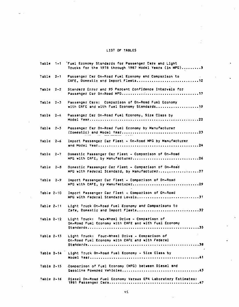
LIST OF TABLES
Table 1-1 "Fuel Economy Standards for Passenger Cars and LightTrucks for the 1978 through 1987 Model Years (in MPG) 3
Table 2-1 Passenger Car On-Road Fuel Economy and Comparison toCAFE, Domestic and Import Fleets 12
Table 2-2 Standard Error and 95 Percent Confidence Intervals forPassenger Car On-Road MPG .' 17
Table 2-3 Passenger Cars: Comparison of On-R-oad Fuel Economywith CAFE and with Fuel Economy Standards 19
Table 2-4 Passenger Car On-Road Fuel Economy, Size Class byModel Year 22
Table 2-5 Passenger Car On-Road Fuel Economy by Manufacturer(Domestic) and Model Year.. 23
Table 2-6 Import Passenger Car Fleet - On-Road MPG by Manufacturerand Model Year 24
Table 2-7 Domestic Passenger Car Fleet - Comparison of On-RoadMPG with CAFE, by Manufacturer 26
Table 2-8 Domestic Passenger Car Fleet - Comparison of On-RoadMPG with Federal Standard, by Manufacturer..... 27
Table 2-9 Import Passenger Car Fleet - Comparison of On-RoadMPG with CAFE, by Manufacturer 29
Table 2-10 Import Passenger Car Fleet -. Comparison of On-RoadMPG with Federal Standard Levels 31
Table 2-11 Light Truck On-Road Fuel Economy and Comparisons toCafe, Domestic and Import Fleets 32
Table 2-12 Light Truck: Two-Wheel Drive - Comparison ofOn-Road Fuel Economy with CAFE and with Fuel EconomyStandards 35
Table 2-13 Light Truck: Four-Wheel Drive - Comparison ofOn-Road Fuel Economy with CAFE and with FederalStandards 38
Table 2-14 Light Truck On-Road Fuel Economy - Size Class byModel Year 41
Table 2-15 Comparison of Fuel Economy (MPG) between Diesel andGasoline Powered Vehicles 43
Table 2-16 Diesel On-Road Fuel Economy Versus EPA Laboratory Estimates:1981 Passenger Cars 47
vi

Table 2-17 On-Road Fuel Economy by Season of Year (Passenger Cars
Plus Light Trucks) 50
Table 2-18 Calendar Year Sales of Light Trucks, Model Years 1979-1981...69
Table 2-19(a) Total Reduction in Fuel Consumption and Dollar EquivalentValue - Passenger Cars and Light Trucks, 74
Table 2-19(b) Per Vehicle Reduction in Fuel Consumption and DollarEquivalent Value - Passenger Cars and Light Trucks 74
Table 3-1 Total Average Vehicle Miles Traveled, as of July 1, 1983,
by Type of Vehicle and Model Year 83
Table 3-2 Standard Deviation and Standard Errors for VMT Estimates 85
Table 3-3 Ninety-five Percent Confidence Limits and Tolerance
Limits on VMT by Vehicle Model Year 88
Table 3-4 Total Vehicle Miles Traveled, Passenger Cars by Size Class....91
Table 3-5 Total Vehicle Miles Traveled, Light Trucks by Size Class 92
Table 3-6 Average VMT Rank by Size Class, Passenger Cars 93
Table 3-7 Vehicle Miles Traveled - Passenger Cars, GasolineVersus Diesel 95
Table 3-8 Total Vehicle Miles Traveled, Gasoline Versus Diesel,
Light Trucks 96
Table 3-9 Comparison of Observed and Predicted VMT 102
Table 3-10 Cumulative and Annual VMT Estimates Based on FittedLogarithmic Curve 105
Table 3-11 Data for Computation of Average Annual VMT, EntireU.S. Fleet of Passenger Cars and Light Trucks 107
Table 3-12 Comparative Estimates of Average Annual Miles Traveled
Per Automobile by Age of Automobile 109
Table 4-1 States Not Sampled (Excluded from Sampling Frame) 119
Table 4-2 Sample Allocation Scheme, Cars and Station Wagons 122
Table 4-3 Sample Allocation Scheme, Trucks 123
Table 4-4 Locator File Disposition1 Codes 129
Table 4-5 Disposition Codes for Returned Questionnaires 130
Table 4-6 Final Dispositions for Total Sample (Based on MailReturns Only) 136
vii

Table D-1 Estimated Vehicle Miles, Lifetime, Passenger Cars 221
Table D-2 Estimated Vehicle Miles, Lifetime, Light Trucks 222
Table D-3 Estimated Average Price of Unleaded Gasoline, 1984 Dollars....226
Table D-4 Disount Factors for Estimating Present Value (1984 Dollars)of Future Reduction in Fuel Consumption 227
viii

LIST OF FIGURES
Figure 2-1 Passenger Car On-Road Fuel Economy Versus CAFE andFederal Standard 13
Figure 2-2 Light Truck (Two-Wheel Drive), On-Road Fuel EconomyVersus CAFE and Federal Standard 33
Figure 2-3 Light Truck (Four-Wheel Drive), On-Road Fuel Economy
Versus CAFE and Federal Standard 40
Figure 2-4 Seasonal Effect on Fuel Economy 51
Figure 3-1 ORFES Vehicle Miles Traveled by Model Year 98
Figure 3-2 Vehicle Miles Traveled Versus Vehicle Age, On-RoadFuel Economy Survey, January-December 1983 100
Figure 4-1 Geographical Distribution of States Not Sampled
(Excluded from Sampling Frame) ". 120
Figure 4-2a On-The-Road Fuel Mileage Log (Questionnaire) 125
Figure 4-2b Reverse Side of Questionnaire 126
ix

ACKNOWLEDGMENTS
The author would like to express his appreciation to the staff at the
National Opinion Research Center (NORC) in Chicago and New York who worked
on the year-long data collection project with its complex schedule of
operations. Special acknowledgment goes to Jean Atkinson, on leave from the
British Office of Population Censuses and Surveys, who guided the NHTSA
survey project from Its initial design phase through most of the data
collection phase.
The author extends, a special note of gratitude to Alleyne Monkman of NHTSA's
Office of Standards Evaluation for her (typical) diligent and faithful
efforts in typing the manuscript.


EXECUTIVE SUMMARY
Over a decade has passed since the 1973 Arab oil embargo which presaged
a worldwide energy crisis. This initial shock was followed by several years
of tight fuel supplies and steadily rising energy prices which had major
impact on the U.S. economy as well as the economies of most other world
countries.
One of the actions taken in response to this energy problem in the
United States was the enactment of the Energy Policy and Conservation Act
(EPCA) in 1975 by the Congress. Among other steps taken by this Act, one
was aimed at energy conservation in the transportation sector through the
establishment of Federal Corporate Average Fuel Economy Standards for new
passenger cars and light trucks. Responsibility for administering this motor
vehicle fuel economy program was assigned to the Secretary of Transportation
who, in turn, delegated it to the Administrator of the National Highway
Traffic Safety Administration (NHTSA). Thus motor vehicle fuel economy
joined motor vehicle safety and other Federal regulatory programs
administered by NHTSA.
Fuel Economy Standards for passenger cars for the first three years
(1978-1980) and for 1985 and thereafter were originally set by the Congress
in the 1975 Energy Policy and Conservation Act. More recently, NHTSA, by
virtue of the statutory authority provided in the 1975 Act, amended the
passenger car standard for Model Year 1986. Also a notice of proposed
rulemaking (NPRM) has been issued concerning revision of the passenger car
standards for Model Years 1987 and 1988. Standards for light trucks have
been established for Model Year 1979 through Model Year 1988. All light
x i i i

truck standards have been set by NHTSA. Chapter 1, (Table 1-1) of this
report lists the individual fuel economy levels, in terms of miles per
gallon, as currently set by the standards.
This study is an assessment of the actual fuesl economy levels, and
reduction in energy consumption of the new, more fuel-efficient vehicles
produced from Model Year 1978 through 1981. It should be noted that, in
addition to the fuel economy standards (which took effect for passenger cars
in Model Year 1978 and for light trucks in Model Year 1979), consumer demand
and other market forces provided incentives for greater fuel economy during
that time period. This study does not attempt to determine what portion of
the improved fuel economy is attributable to the Federal standards.
A second major portion of this study develops estimates of annual
vehicle miles traveled (VMT) by age and type of vehicle (passenger car and
light truck) using vehicle odometer readings. It is believed that this is
the first time that estimates of VMT have been developed using actual
odometer readings from a large-scale national sample of the U.S. vehicle
fleet.
The study was conducted to comply both with Executive Order 12291
concerning the review of Federal regulations, and with NHTSA's regulatory
review plan published in March 1982 (Regulatory Reform - The Review
Process).
xiv

As with most of NHTSA's evaluation studies, data reflecting
"real-world" or "on-road" experience are used. The data come from a
specially conducted survey, using probability sampling methods, of the
Nation's fleet of privately owned and operated passenger cars and light
trucks. Vehicle owner/drivers provided fuel-mileage logs or diaries for
approximately 9,000 vehicles. Each log contained data on fuel purchases and
odometer readings for approximately a one-month period. The sample was
fielded in twelve monthly replicates throughout an entire one year period
in order to account for seasonal effects on fuel economy and on vehicle
travel.
This study is not an evaluation or assessment of official compliance
with the Federal fuel economy standards. The process by which official
compliance is determined was established via statute as part of the Energy
Policy and Conservation Act of 1975 which authorized the standards. For
each manufacturer, the Environmental Protection Agency (EPA) computes an
overall average fuel economy for each model year. This overall average fuel
economy (or miles per gallon) is based on laboratory measurements generated
by the EPA during its testing of vehicles for emissions levels and for
determining compliance with Federal emissions standards. Fuel economy
measurements are made for each basic vehicle type for each manufacturer and
a harmonically weighted average figure is calculated based on the number of
vehicles of each basic type sold by each manufacturer within each model
year. This overall fuel economy is thus a sales-weighted average and is
commonly referred to as the corporate average fuel economy, or "CAFE." It
is this CAFE which determines official compliance with the Federal fuel
economy standards.
-XV

While the laboratory results generated by the EPA provide a
standardized controllable, repeatable, convenient, and economical (i.e., the
production of fuel economy data as a byproduct of emissions testing was
already in place prior to enactment of the ECPA in 1975) method of assessing
manufacturer progress vis-a-vis the Federal standards, it has nonetheless
been well established by several prior studies1 that laboratory tests do not
necessarily reflect fuel economy under typical, everyday driving conditions;
laboratory results are typically higher than actual on-road fuel economy.2
Also as has been noted previously, it has been the policy of NHTSA to
utilize data reflecting actual "on-road" experience, wherever feasible in
its studies of the effects of its programs and motor vehicle regulations.
The general objectives of this study are to:
(1) Estimate the on-road fuel economy improvements for passenger
cars and light trucks produced from the beginning of fuel
economy standards through Model Year 1981.
(2) Compare the on-road fuel economy with the respective
laboratory-based, or corporate average fuel economy (CAFE)
levels as computed by the Environmental Protection Agency
and as specified in the Energy Policy and Conservation Act of
1975.
1 These studies have been done'both by other Federal agencies and by companieswithin the motor vehicle industry. The results of these studies arediscussed later in this report.
2 Largely as a consequence of this situation, the EPA has recently begundiscounting its laboratory data on fuel economy which are displayed on"window stickers" of new motor vehicles and which are published in the EPAannual consumer booklet, "Gas Mileage Guide."
xvi
(3) Compare the on-road fuel economy with the levels set by the
respective Federal Fuel Economy Standards. ..-••
(4) Estimate the reduction in energy (fuel) consumption, and
dollar equivalent value, for vehicles produced from Model
Year 1978 through Model Year 1981.
(5) Estimate annual vehicle miles traveled by the U.S. fleets of
passenger cars and light trucks, by age of the vehicle and
overall average per vehicle.
FINDINGS AND CONCLUSIONS
Following are the principal findings and conclusions reached in this
study:
(1) On-Road Fuel Economy of Passenger Cars
a. From Model Year 1978 through 1981, the on-road
fuel economy of the U.S. fleet of passenger cars
increased by 41 percent, rising from 15.2 mpg in Model
Year 1977 to 21.4 mpg in Model Year 1981.
b. The greater portion of this gain in fuel economy is
attributed to the domestic fleet (39 percent gain)
compared to the import fleet (13 percent gain). This
is to be expected considering the large differences in
the original size and fuel economy of the two fleets
xvi i

prior to promulgation of the standards, and prior to
the significant increase in fuel prices following the
"second oil shock" of 1979.
c. Among domestic manufacturers, overall fuel economy
gains for the four model year period ranged from a low
of 25 percent for American Motors to a high of 70
percent for Chrysler, which had a large jump of nearly
6 mpg from Model Year 1980 to Model Year 1981.
d. Gains among foreign manufacturers were modest except
for Volkswagen's 30 percent increase, from the 1977 to
1981 models, attributable to a large penetration of
diesel vehicles.
(2) On-Road Fuel Economy of Light Trucks
a. From Model Year 1979 through 1981, on-road fuel
economy increased by 26 percent (13.4 mpg to 16.9 mpg)
for 2-wheel drive vehicles; for 4-wheel drive trucks,
the increase was 17 percent (12.3 mpg to 14.4 mpg).
xviii

b. As was true for passenger cars, fuel economy gains
were greater for domestic vehicles. The relative
gains from 1978 to 1981 model fleets were:
2-wheel drive Change in MPG
domestic trucks: +21% mpg
import trucks: +9* mpg
4-wheel drive
domestic trucks: +9% mpg
import trucks: +495 mpg'
(3) On-Road Fuel Economy Compared to Laboratory-based (EPA) CAFE*
a. For the model years surveyed, on-roa'd fuel
economy is consistently below laboratory-based CAFE
levels. For passenger cars the difference is 15
percent; for 2-wheel drive trucks, 16 percent; for
4-wheel drive trucks, almost 20 percent.
3 1980 to 1981 increase4 It should be noted that the EPA recently issued a final rule (50 FR 27172,
July 1, 1985) adjusting its fuel economy measurements for Model Year 1980and later, to account for test procedure changes. While this informationwas not available at the time this study was written, the effect of this EPAadjustment is to increase somewhat the differences between EPA CAFE valuesand on-road fuel economy, as estimated in this study, for Model Years 1980and 1981.
xix

b. Except for 4-wheel drive trucks, domestic vehicles
exhibited a somewhat greater difference than import
vehicles.
c. The CAFE to on-road difference among domestic
manufacturers was approximately the same with AMC and
Chrysler showing slightly less difference than GM and
Ford.
d. Among import vehicles, the greatest CAFE to on-road
difference was noted for the captive imports of Ford
and Chrysler. Only one manufacturer, Volkswagen, had
an on-road mpg consistently at or above its CAFE.
e. This finding that on-road fuel economy is consistently
below laboratory-based CAFE is not new. It has been
shown in several prior studies although the data
bases used and the magnitudes of the CAFE to on-road
differences found have differed somewhat from those in
this study. This study is believed to be the first
which develops on-road fuel economy estimates from a
nationwide, large-scale probability sample.of the
total national population of privately-owned vehicles.
XX

(4) On-Road Fuel Economy Compared to Federal Fuel EconomyStandards
a. For the three categories of vehicles, passenger cars,
two-wheel drive trucks, and four-wheel drive trucks,
the on-road fuel economy ranges from 8 to 9 percent
below the Federal standard levels for Model Years
1978-1979; for 1980-1981, on-road mpg is much closer
to the standard levels and in some instances, slightly
above.
b. Domestic vehicle on-road mpg is approximately 10
percent below the Federal standards; import vehicle
on-road mpg ranges from 20 to 45 percent above the
Federal standards. As stated earlier, this is
primarily due to the smaller average size of import
vehicles compared to the average size of domestic
vehicles. Relative fuel economy gains were greater
for domestics than for imports.
(It should be noted, as previously stated, that
compliance with the Federal standards is determined
through laboratory testing by the Environmental
Protection Agency. All vehicles, both import and
domestic, complied with the Federal Standards during
the study period).
XXI

(5) Estimated Reduction in Energy Consumption and Dollar
Equivalent Value
a. Estimated, vehicle lifetime, reduction in energy
consumption and dollar equivalent value (in 1984
dollars) for all vehicles (cars and trucks)
manufactured under the Federal standards through Model
Year 1981 are:
Reduced FuelConsumption Dollar Value
Total 45.6 billion gallons $53.8 billion(All vehicles) (1.1 billion barrels)
PerVehicle 974 gallons $1,146
The baseline periods for these estimates are Model
Year 1977, for passenger cars, and Model Year 1978,
for light trucks.
Costs of implementing the Federal fuel economy
standards were not estimated for reasons described in
the report.
xxn
6. Vehicle Miles Traveled
An analysis of odometer readings for the approximately 9,000
vehicles covered in the survey gave the following estimates
concerning vehicle miles of travel by the Nation's population
of privately owned vehicles:
a. Average annual miles of travel for passenger cars and
light trucks is essentially the same — approximately
6,000 miles per year for the average vehicle.
b. Average annual miles of travel show little differences
of a practical nature between classes of vehicle
(e.g., small versus large car; 2-wheel drive versus
4-wheel drive truck, etc.).
c. Average annual miles of travel per vehicle shows a
sharp decline with vehicle age. First year travel is
estimated at 14,000 miles, but by the fifth year of
age, travel drops to less than half, or about 6,500
miles.
d. Total miles traveled was found to be considerably
higher for diesel vehicles than for conventionally
powered gasoline vehicles. This difference was more
pronounced for passenger cars than for light trucks.
Also, in contrast to the finding for the overall
fleet, vehicle size appeared to be an important factor
xx i i i

here as well, with small diesel powered vehicles
showing a greater increase in miles driven over their
gasoline powered counterparts, than large diesel
powered vehicles.
e. Average annual travel estimates from the On-Road
Survey are similar to estimates of other prior
surveys for the initial few years of vehicle life.
For later years, however, the On-Road results show a
much greater rate of decline in average annual travel
than prior surveys.
f. Results from the On-Road Survey indicate that average
annual travel per passenger car or light truck, and
total travel for all vehicles may be substantially
lower than heretofore estimated. Although fleet and
business use vehicles were not Included in the survey,
travel by this class of vehicles does not appear to be
of sufficient magnitude to account for the lower VMT
(vehicle miles traveled) findings in this study.
This is believed to be the first study to develop VMT
estimates from odometer readings of a large national
probability sample of the Nation's population of privately
owned passenger cars and light trucks.
XXIV

CHAPTER 1
INTRODUCTION
This is one of the continuing series of studies that have been
conducted by the National Highway Traffic Safety Administration (NHTSA) to
review and evaluate the effects of existing Federal regulations and programs
for which the Agency is responsible. Following the issuance of Executive
Order 12291 on February 17, 1981, the NHTSA developed and published a
regulatory review plan1 which contained a description of those regulations
selected for review together with a schedule for the conduct of the
individual reviews. The Automotive Fuel Economy Program was listed in that
review plan under the category of "moderate to high" priority.
The purpose of the Automotive Fuel Economy Regulations was to conserve
petroleum energy through the production of more fuel efficient motor
vehicles. These regulations were authorized under the Energy Policy and
Conservation Act of 19752 which grew out of the Arab oil embargo of late
1973. The fuel economy regulations, along with other parts of the Energy
Policy and Conservation Act, were part of a concerted National effort to
reduce energy consumption in the face of suddenly scarce petroleum supplies
and skyrocketing prices which grew out of the Arab oil embargo.
^ "Regulatory Reform - The Review Process," U.S. Department of Transportation,National Highway Traffic Safety Administration, March 1982 (DOT HS-806-159).
2 Public Law 94-163, Title III, "Improving Energy Efficiency." This sectionof the legislation amended the existing Motor Vehicle Information and CostSavings Act through the addition of Title V, "Improving AutomobileEfficiency. It is this latter portion of legislation which authorized thedevelopment and implementation of a multi-year program (i.e., thepromulgation of Federal fuel economy standards) to improve the fuel economyor passenger cars and light trucks sold in the United States.

The Energy Policy and Conservation Act assigned the responsibility for
administering the fuel economy program to the Secretary of Transportation,
who, in turn, delegated this responsibility to the Administrator of the
National Highway Traffic Safety Administration on June 22, 1976 (A1 F.R.
25015).
NHTSA's responsibilities, under the Act, include:
(1) establishing average fuel economy standards for manufacturers
of passenger automobiles and light trucks,
(2) promulgating .regulations concerning procedures, definitions,
and reports necessary to support the "fuel economy standards,
(3) considering petitions for exemption from established fuel
economy standards by low-volume manufacturers (e.g., those
whose total production is less than 10,000 vehicles
annually), and establishing alternative standards for these
manufacturers,
(A) reporting annually to Congress on the progress of the fuel
economy program,
(5) enforcing the fuel economy standards and regulations, and
(6) responding to petitions concerning domestic production by
foreign manufacturers and other matters.

The fuel economy standards that have been established through 1986appear in Table 1-1.
TABLE 1-1
Fuel Economy Standards for Passenger Cars and Light Trucksfor the 1978 through 1987 Model Years (in MPG)
ModelYear
19781979d
1980e
1981*198219831984198519861987
PassengerCars - MPG
18.0c
19.0c
20.0c
22.024.026.027.027.5C
26.0f
27.5C> 9
Two-WheelDrive
17.216.016.718.019.520.319.720.521 .0
Light Trucksa
MPGFour-Wheel
Drive-Not Establlshed-
15.814.015.016.017.518.518.919.519.5
Composite13
17.2
17.519.020.019.520.020.5
a - Standards for 1979 model year light trucks were established for vehicleswith a gross vehicle weight rating (GVWR) of 6000 lbs. or less. Standardsfor MY's 1980 through 1985 are for light trucks with a GVWR of up to 8,500lbs.
b - For model years 1982-1986 manufacturers may comply with the two-wheel andfour-wheel drive standards or may combine their two-wheel and four-wheeldrive light trucks and comply with the combined standard.
c - Established by Congress in the Energy Policy and Conservation Act of 1975.
d - For MY 1979, light truck manufacturers may comply separately with standardsfor four-wheel drive, general utility vehicles and all other light trucks,or combine their trucks into a single fleet and comply with the 17.2 mpgstandard.
e - Light trucks manufactured by a manufacturer whose fleet is poweredexclusively by basic engines which are not also used in passenger auto-mobiles, must meet standards of 14 mpg and 14.5 mpg in model years 1980 and1981, respectively.
f - The Energy Policy and Conservation Act of 1975 originally established astandard of 27.5 mpg for 1985 and subsequent years, but also provided theDepartment of Transportation with authority to amend that standard. InOctober 1985, NHTSA issued a final rule which changed the 1986 standard to26.0 mpg.
g - For Model Year 1987 and subsequent years. (Rulemaking action is presentlypending which would revise the standards for Model Years 1987 and 1988).
Sources: "Automotive Fuel Economy Program, Seventh Annual Report toCongress," U.S. Department of Transportation, National HighwayTraffic Safety Administration, January 1983.
"49 FR 41250," October 22, 1984

It should be noted that the standards began in 1978 for passenger cars and
in 1979 for light trucks; also to be noted is that certain standard levels
for passenger cars were "pre-established" by the Congress as part of the
authorizing legislation of 1975, whereas all remaining standard levels for
passenger cars and all standards for light trucks were the responsibility of
the Department of Transportation (DOT). Within certain guidelines, the Act
also provided the DOT with the authority to revise pre-set standard levels
for future model years, should such revision be deemed appropriate.
This study addresses the actual, on-road reduction energy, or fuel,
consumption for the U.S. fleet of passenger cars and light trucks produced
from the beginning years (1978 for passenger cars; 1979 for light trucks) of
the fuel economy standards through 1981. The study deviates, somewhat, from
the typical NHTSA evaluation study, or review, of a major regulation or
safety program where the primary focus is to estimate the effectiveness, or
benefits, attributable to that program and to compare these benefits to the
costs of Implementing the program. There are two reasons why the
conventional approach to program evaluation was not employed in this study.
First, although original plans called for estimation of costs of
implementing the Federal fuel economy regulations, subsequent budgetary and
program changes precluded the execution of this part of the evaluation
effort. In addition, it was recognized that the pervasive scope and complex
nature of the changes made within the motor vehicle industry in the drive
for greater fuel efficiency would make the estimation of the costs of
implementing the regulations difficult indeed. In addition to specific
technological developments such as diesel engines and improved

.transmissions, essentially all major domestic carline's were redesigned and
"downsized"; the use of front-wheel drive became widespread. It would have
been extremely difficult to attribute, objectively, the cost of such
comprehensive changes to the goal of increased fuel economy, vis-a-vis other
goals such as styling changes, improvements in vehicle quality and
reliability, etc. It is not difficult, therefore, to see that the isolation
of the costs of implementing the fuel economy regulations would be a task of
emminently greater complexity than the estimation of costs for motor vehicle
safety'standards such as side door beams, energy absorbing steering
assemblies, or fuel system integrity improvements, whose costs have been
estimated as parts of prior NHTSA evaluation studies.
A second reason complicating the traditional benefits versus costs3
approach to this study was that it would be difficult to attribute the
reduced fuel consumption of the vehicles produced subsequent to the
effective dates of the fuel economy standards to the standards themselves.
In addition to the Federal requirements to manufacture vehicles with better
fuel economy, there was also a second incentive in the form of increased
market or consumer demand for such vehicles, since gasoline prices had
increased dramatically during the 1970's and early 1980's.
While the cost effectiveness of the CAFE standards per se have not beenevaluated, NHTSA, as part of its Regulatory Impact Analysis of each CAFEstandard promulgated, has analyzed the cost effectiveness of the fuelefficiency improvements available at that time to the manufacturers. Thecost effectiveness of fuel efficiency improvements is defined as theestimated retail price increase to consumers, of the vehicle changes, versusthe present discounted value of fuel saved over the vehicle's lifetime.These analyses showed that cost-effective fuel efficiency improvements wereavailable.
These analyses were "before the fact" (i.e., conducted prior to the actualproduction and sale of the vehicle) whereas the analysis in this study isafter the fact, covering vehicles that are on the road and that havegenerated real-world experience.

As is true for most NHTSA evaluation studies,.emphasis is placed on
assessing the effects of agency regulations, in this case, fuel economy
regulations, through the collection and analysis of real-world data. The
data for this study was gathered through a nationwide, on-the-road survey of
the fuel economy experienced by the U.S. fleet of Model Year 1977 through
1981 passenger cars and light trucks. The target population was also
defined as those vehicles manufactured by the four major domestic companies
and the four major foreign companies (Datsun/Nlssan, Honda, Toyota, and
Volkswagen) and was restricted to vehicles owned by private individuals
(i.e., fleet vehicles excluded). The survey was based on a national
probability sample with the sampling frame being the national vehicle
registration files maintained by the R. L. Polk Company. The sample was
stratified by model year of vehicle, vehicle type (passenger car, light
truck) vehicle size class (subcompact, compact, midsize, etc.), fuel type
(gasoline, diesel), and, for light trucks only, the number of drive wheels
(two-wheel drive, four-wheel drive). The final sample included 100 strata.
Allocation of the sample among strata for each model year and vehicle type
was made on a proportional basis with oversampling employed in a few
instances for rare strata in order to obtain reasonable subsample sizes in
the final sample. Allocation of the sample, within each stratum was also
made on a proportional basis among all of the individual vehicle make model
combinations comprising each stratum. Over 800 different vehicle make
models (i.e., 1961 Oldsmobile Cutlass diesel, 1981 Ford Escort, etc.) appear
in the final respondent sample (see Appendix A). The total sample was
subdivided into twelve equal replicates with one replicate being fielded for
each month of the data collection period, Calendar Year 1983. This

distribution over a 12-month period provided control over the seasonal
effect on fuel economy and vehicle miles traveled. Each vehicle stratum was
distributed equally within each of the 12 replicates.
The methodology for carrying out the survey consisted of mailing a
request to owners of sampled vehicles to maintain a record or diary4, of
their fuel purchases and respective odometer readings over a specified,
1-month period. To enhance survey response, the record-keeping request was
preceded by an advance notification letter, and accompanied by a small
incentive in the form of a log-booklet for the respondents' personal use
plus "reminder decals." Two follow-up "reminder" postcards were also sent,
one shortly after the mailing of the log-questionnaire and the second at the
end of the survey month to remind the respondent to return the completed
survey log. A second wave of mailings, including the questionnaire letter
and reminder postcards, were sent to all sampled owners who failed to
respond to the initial survey wave. Finally, telephone followup samples
were taken to investigate the potential effect of nonresponse and to assess
the potential for the telephone to enhance basic survey response. A more
detailed discussion of the survey methodology is given in Chapter 4.
The data collection and data automation phases of the On-Road Fuel
Economy Survey (ORFES) were conducted for NHTSA by a survey contractor.*
The contractor also provided certain computations and tabulations from the
data as well as completing a report on potential effects of survey
nonresponse.
* See Chapter A for a specimen of the survey instrument and Appendix Cfor other survey materials.
5 "On-the-Road Fuel Economy Survey - Final Data Collection Report", submittedto NHTSA, Office of Program Evaluation, by National Opinion Research Center,October 1984.

The initial total sample of vehicles selected from the "Polk" sampling
frame was 46,000. Out of this, a total of 8,914 vehicles were represented
on the final survey analysis data file for a conservatively estimated
response rate of 21 percent. However, when the results of the two telephone
samples are considered together with the definition of eligible respondents
as agreed upon by the Council of American Survey Research Organizations6,
the effective response rate is in the vicinity of 35-40 percent. Survey
response as well as explanations of the data automation procedures, quality
control, etc., are also presented in Chapter 4.
Although the original primary objective of the ORFES was to estimate
on-road fuel economy, it was recognized that the survey would provide a
large sample of actual vehicle odometer readings from which estimates of
vehicle miles traveled could be developed. Data on vehicle miles traveled
are also of considerable interest to NHTSA, as well as several other
agencies. Thus a second important area covered in this report is the esti-
mation of annual vehicle miles of travel by age of vehicle, by passenger car
and light truck, and by vehicle size class. These estimates are compared
with vehicle miles traveled estimates from prior known surveys and studies.
This report is presented in the four chapters which follow. Chapter 2
contains the results on fuel economy as measured in the on-road survey. In
this chapter, comparisons are also made between the on-road fuel economy and
6 See Chapter 4, Section 4.4.
respective EPA CAFE7 numbers and between on-road fuel economy and the
Federal standards. Also in Chapter 2, the effect of seasonallty and certai.fl
vehicle technologies on in-use fuel economy are analyzed. Thirdly, this
chapter contains a comparison of the ORFES on-road results with several
prior studies of on-road fuel economy. Chapter 2 concludes with an analysis
of the reduction in energy (fuel) consumption, and dollar equivalent value
for the vehicle fleet produced subsequent to enactment of the Federal
standards up through Model Year 1981. Chapter 3 contains the results of the
vehicle miles traveled estimates as developed from the survey data on
odometers and compares the ORFES estimates with those of prior studies and
surveys of vehicle miles traveled. Chapter 4 describes the survey design
data collection, data automation, survey response and nonresponse analysis.
Chapter 5 summarizes the primary findings and results from an analysis of
the survey data as it relates to fuel economy and vehicle miles traveled.
7 CAFE or Corporate Average Fuel Economy as defined in the Energy Policy andConservation Act of 1975, is that number which is used to determine eachmanufacturer's compliance, for a given model year, with the Federal fueleconomy standard for that year. The CAFE is a number which is thesales-weighted harmonic mean of the fuel economy (mpg) of all individualbasic vehicle types produced by a manufacturer in a given model year and Iscomputed by the Environmental Protection Agency based on its laboratorytests of new vehicles for purposes of determining compliance with Federalemissions standards.

CHAPTER 2
ANALYSIS OF SURVEY RESULTS OF FUEL ECONOMY AND ESTIMATIONOF REDUCED ENERGY CONSUMPTION AND EQUIVALENT DOLLAR VALUE
2.0 INTRODUCTION
This chapter contains the analysis and summary of the fuel economy
results as reported by vehicle owners/drivers in the nationwide On-The-Road
Survey. Chapters 1 and A contain descriptions of the survey design and
methodology, survey Instrument and materials, data collection, data
automation and quality control, survey response, and nonresponse/noncoverage
effects.
All fuel economy estimates presented In this chapter, except where
otherwise noted, are harmonically weighted means1 using, as the weights,
actual nationwide counts of vehicles on the road as compiled,from national
vehicle registration files.2 These estimates are analogous to the
harmonically weighted means using sales data, as specified in the Energy
Policy and Conservation Act of 1975, which established the Federal Fuel
Economy Standards Program for passenger cars and light trucks.
1 See Chapter 1, footnote 7.2 Vehicle counts are taken from the files compiled by the R. L. Polk Company
as of July 1, 1962, the latest data available when the analyses of data wereinitiated.
10
The on-road fuel economy results are presented by type of vehicle
(passenger car, light truck); vehicle origin of manufacture (domestic,
import); vehicle manufacturer3; and vehicle size class (essentially
corresponding to EPA size class). Data are also presented to compare fuel
economy between gasoline and diesel powered vehicles.
Secondly, comparisons are made between on-road fuel economy and
laboratory based (EPA) corporate average fuel economy (CAFE) levels, and
between on-road fuel economy and the applicable Federal standard levels.
~ Third, and lastly, estimates of the total reduction in energy
(fuel) consumption are made for the vehicles represented in the survey, both
on an overall vehicle lifetime basis, and on a per vehicle (lifetime) basis.
Estimated dollar equivalent values of the reduced consumption are also
developed.
2.1 PASSENGER CARS: ON-ROAD FUEL ECONOMY
Table 2-1 displays the on-road fuel economy for passenger cars for
the 5 model years covered by the survey. Data are shown for both the
Domestic'Fleet, the Import Fleet and the overall or combined U.S. Fleet.
Also presented are the respective EPA CAFE's and the Federal Fuel Economy
Standards for the 4 years, 1978 through 1981. Figure 2-1 displays the trend
in on-road, EPA CAFE, and standard values by model year.
The survey included all four major domestic manufacturers (including theircaptive imports, as appropriate), plus the four major foreign manufacturers(Datsun/Nissan, Honda, Toyota and Volkswagen).
11

TABLE 2-1
PASSENGER CAR ON ROAD FUEL ECONOMYAND COMPARISON TO EPA CAFE
- DOMESTIC AND IMPORT FLEETS -
FLEETMiles per Gallon for Model Year:
1977 1978 1979 1980 1981
DomesticOn-RoadEPA CAFE
ImportEPA On-Road
CAFE4
Overall On-RoadOverall EPA CAFE5
Fuel EconomyStandard
U.5N/A
23.7N/A
15.218.6
N/A
15.718,7
24.628.7
16.619.9
16.0
16.519.3
25.027.2
17.320.3
19.0
18.621. B
26.729.7
20.023.4
20.0
20.223.6
26.731.4
21.425.2
22.0
NOTE 1: Sample sizes (i.e., number of vehicles reporting in the nationalsurvey) ranged from 109 to 1,527 for each of the ten subgroups inthe above table.
NOTE 2: The above EPA CAFE values were correct at the time this study waswritten. However, it should be noted that the EPA recently Issueda final rule (50 FR 27171, July 1, 1965) which adjusted (upward)its fuel economy measurements for Model Year 1980 and later, toaccount for changes in test procedures. The effect of this EPArevision Is to increase, somewhat, the above CAFE's for Model Years1980 and 1981, and thereby increasing the amounts of CAFE toon-road differences as estimated in this study.
CAFE for six import manufacturers included in survey: Datsun/Nissan, Honda,Toyota, Volkswagen, and two captive import groups, Chrysler and Ford.CAFE for all import manufacturers, Including captive imports for Chryslerand Ford.
12

As the table shows, the overall (i.e., total fleet) on-road fuel
economy shows a steady improvement over the base 1977 Model Year from 15.2
miles per gallon (mpg), to 21.4 mpg for the 1961 Model Year. This repre-
sents a total increase in fuel economy of 6.2 mpg or 41 percent over four
model years. The yearly, average increase amounts to approximately 10
percent or 1.55 mpg. The major portion of this increase can be attributed
to vehicles produced in the U.S. which saw an overall increase in fuel
economy of approximately 40 percent, compared to an increase of 13 percent
for the imports. Of course, it must be remembered that prior to enactment
of the fuel economy regulations, the mpg was considerably higher for the
imports than for domestically manufactured cars; import fleet mpg for the
base year was nearly 60 percent higher than domestic fleet mpg. Conse-
quently, the impetus for import manufacturers to raise mpg was less since
their base year mpg was already higher than the fuel economy regulations
called for, even as late as 1981.
One qualifying comment should be noted in the above discussion of
the fuel economy improvements. Nineteen seventy-eight was the initial year
of the Federal Fuel Economy Regulations, and therefore, 1977 is taken as the
base year on which to compute fuel economy gains. However, the first
significant step to increase passenger car fuel efficiency came in the 1977
model year when General Motors downsized its standard-sized cars and
standard-sized station wagons. Based on registration data, the GM standard
size cars accounted for approximately 20 percent of the U.S. domestic fleet
of 1977 passenger cars. Therefore, it may be stated that the above
estimates of total fuel efficiency gains are somewhat conservative since
they do not include that portion of the gain resulting from the downsizing

of the 1977 GM standard size cars. As noted previously, Model Year 1977 was
the earliest year covered by the survey and thus the actual Incremental
savings attributable to the downsized GM standard vehicles cannot be
measured with the available data.
2.1.1 RELIABILITY OF ON-ROAD FUEL ECONOMY ESTIMATES
In statistical surveys such as the On-Road Fuel Economy Survey, it
is typically of Interest to estimate not only the mean values for certain
population parameters — in this case, on-road fuel economy or mpg—but also
to evaluate the reliability of these estimates. Reliability here is defined
as the degree of precision which can be attached to the various mean
estimates.
The standard method of measurement of precision in statistical
surveys is the standard error which in the simple case'is the sample
standard deviation, s, divided by the square root of the sample size, or n.
Table 2-2 contains standard error estimates for each of the overall model
year (e.g., domestic plus import) estimates of on-road mpg as given in Table
2-1. The standard errors for each model year are estimated from the
formula:
SE(Model Year) =
15

where,
SEn = s/S/n s standard error for each stratum in the sample or
each vehicle size class within a given model
year.
and Wh c weighting factor corresponding to the proportion of the
total vehicle population in the stratum/size class
relative to the total vehicle population for the given
model year.
Also given in the table are the 95 percent confidence intervals
for the mean estimates for each model year. The interpretation for each of
these intervals is that in repeated sample surveys such as this, 95 percent
of intervals so constructed would contain the true population mean or the
true on-road mpg for the particular model year.
16

TABLE 2-2
STANDARD ERROR AND 95 PERCENT CONFIDENCE INTERVALSFOR PASSENGER CAR ON-ROAD MPG
ModelYear
1977
1978
1979
I960
1981
SampleSize
B55
1, 129
1,380
1,570
2.1U
On-RoadMPG (Mean)
15.2
16.6
17.3
20.0
21.A
StandardError (MPG)*
0.157
0.U5
0.184
0.132
0.120
RelativeStandardError (%)
1.0
0.9
1.1
0.7
0.6
95 PercentConfidenceInterval (MPG)»
14.9 - 15.5
16.3 - 16.9
16.9 - 17.7
19.7 - 20.3
21.2 - 21.6
•It will be recalled that the mean mpg has been calculated using theharmonic formula since this was the method specified in the Energy Policyand Conservation Act which established the CAFE standards. The standarderrors in the above table however, have been computed on the basis of aregular arithmetic mean due to the general lack of computerized statis-tical algorithms to handle standard errors for harmonic means. (It hasfor years been nearly universal in the fields of analytical and surveystatistics to utilize the arithmetic mean rather than the harmonic meanas a measure of central tendency.) Since it can be shown that theharmonic mean, in the general case, is slightly less than the arithmeticmean, it follows that an "arithmetic standard error" will be slightlyless than a "harmonic standard error." This is due to the fact that thestandard error is a function of > **^ - x ) 2 , or the sum of squaresof the deviations of the sample mean from each individual sampleobservation. Also confidence intervals constructed from arithmeticstandard errors will be slightly more narrow than similar intervals basedon harmonic standard errors. However, the magnitude of such differenceswill be quite small for the data collected in the On-Road Survey andhence the estimates given in the above table will be very close to thevalues that would be obtained based on "harmonic standard errors."
17

It can be seen that the magnitude of the standard error does not
differ appreciably among the five model years, ranging from 0.12 to 0.18.
Relative to the mean however, it is seen that the error does tend to
decrease with the later model years.
2.1.2 ON-ROAO FUEL ECONOMY VERSUS EPA CAFE
Table 2-3 compares the results from the On-Road Survey with the
CAFE (as based on EPA test data) and with the Federal Fuel Economy Standards
for the years 1978-1981.
For the domestic cars, the on-road experience is consistently
below respective EPA CAFE levels by about 15 percent. On an absolute, or
mpg basis, the difference is somewhat larger in 1981 than in the period
1978-1980, rising to 3.4 mpg from about 3.0 mpg. This is to be expected if
the relative difference is essentially constant over the 4 years since both
the on-road and EPA CAFE levels show continual increases.
For imported cars, the on-road fuel economy is closer to the EPA
CAFE than for the domestic vehicles. No clear trend Is evident here,
however, since the on-road mpg is 14 to 15 percent lower-than the EPA CAFE
for Model Years 1978 and 1981, but only 8 to 10 percent, for the intervening
years 1979 and 1978. On an absolute basis, import on-road mpg is below the
EPA CAFE, ranging from approximately 2 to 5 mpg less. Again no distinct
trend is evident.
18

TABLE 2-3
PASSENGER CARS:COMPARISON OF ON-ROAD FUEL ECONOMY WITH EPA CAFE
AND WITH FUEL ECONOMY STANDARDS
COMPARISON 1978 1979 1980 1981
.. MPG PERCENT MPG PERCENT MPG PERCENT MPG PERCENT
Domestic vs.
EPA CAFE [3.0] [16.0] [2.B] [14.5] [3.2] [14.7] [3.4] [14.4]
Import Fleet vs.EPA CAFE [4.1] [14.3] [2.2] [8.1] [3.0] [10.1] [4.7] [15.0]
Overall Fleet vsEPA CAFE [3.3] [16.6] [3.0] [14.8] [3.4] [14.5] [3.8] [15.1]
Domestic vs.Standard [2.3] [12.8] [2.5] [13.2] [1.4] [7.0] [1.8] [8.2]
Import vs.Standard 6.6 36.7 6.0 31.6 6.7 33.5 4.7 21.4
Overall Fleet vs.Standard [1.4] [7.8] [1.7] [8.9] 0.0 0 [0.6] [2.7]
NOTE: Bracketed entries represent negative values (i.e., on-road valuesless than respective EPA CAFE or standard values).
On a relative overall fleet (e.g., both domestic and import
vehicles combined) basis, the on-road mpg is below the respective EPA CAFE
by about 15 percent or 3-4 mpg. These differences are quite close to the
differences noted for the domestic vehicles and, again, are to be expected
since domestic vehicles comprise the major portion of the U.S. passenger car
fleet.
19

2.1.3 ON-ROAD FUEL ECONOMY COMPARED TO THE FEDERAL STANDARDS
Table 2-3 also compares the on-road mpg with the Federal Standards
for the 4 model years, 1978-1981. As shown, the domestic fleet Is below the
Standard for each of the 4 years, by an average of 10.3 percent, or 2.0
miles per gallon. There is some indication that this difference may be
declining for the later model years (e.g., 1980-1961).
Imports, on the other hand, show an on-road mpg considerably above
the Federal standards, ranging from 21 to 37 percent (5-7 mpg) above the
standard levels. As pointed out earlier, however, the imports average
on-road mpg was originally (i.e., prior to enactment of the Federal
standards) at a level considerably above the level required by the
standards, as those vehicles have been, and remain, predominately small
cars.
On an overall fleet basis, the difference between on-road mpg and
the Federal standard levels appears to be narrowing, with the 1980-81
difference being about 1.5 percent compared to 8-9 percent in 1978-79. On
an mpg basis, this difference for 1980-81 averages less than one-half mile
per gallon, with the on-road average for 1980 exactly equaling the standard
level of 20.0 miles per gallon.
20

2.1.4 ON-ROAD FUEL ECONOMY BY VEHICLE SIZE CLASS
Table 2-4 displays the on-road fuel economy by vehicle size
class.6 From 1977 through 1981, consistent year-to-year gains were made for
most size classes. Over the full 4-year period, the average increase in mpg
per size class was 35 percent. The largest gain (79 percent) was registered
for the compact class, while the mini class had the lowest increase at 7
percent.
2.1.5 ON-ROAD FUEL ECONOMY BY MANUFACTURER
Tables 2-5 and 2-6 display the on-road fuel economy (MPG) by model
year for the domestic manufacturers and the import manufacturers,
respectively. The import table also includes "Ford" and "Chrysler" which
refer to the captive imports for these two manufacturers. These are broken
out since captive imports are to be treated separately (i.e., not combined
with vehicles manufacturer domestically) in accordance with the legislative
6 The size classes here essentially correspond to the EPA size classes asdefined In the annual "Gas Mileage Guide" publications for the respectivemodel years covered by the survey. One exception is the "mini" class whichincludes not. only vehicles classified as "mini", but also vehiclesclassified as "two-seaters."
21

TABLE 2-4
PASSENGER CAR ON-ROADFUEL ECONOMY
SIZE CLASS BY MODEL YEAR
Miles per Gallon for Model Years:
Size Class
Mini
Sub-Compact
Compact
Midsize
Large
Small StationWagon
Midsize StationWagon
Large StationWagon
1977
22.9
17.4
14.5
14.3
13.6
1976
21.0
21.2
16.4
15.2
14.5
1979
22.3
21.3
16.2
16.0
15.4
1980
23.4
23.3
19.1
1S.2
16.4
1981
24.5
24.3
25.9
19.6
17.6
19.2
13.9
21.0 21.5 24.0 25.4
15.7 16.2 17.2 19.7
13.0 14.3 14.0 15.8 16.5
NOTE: Sample sizes range from 19 to 491 vehicles for each of the 40 Size
Class-Model Year categories.
22

TABLE 2-5
PASSENGER CAR ON-ROAD FUEL ECONOMY BY MANUFACTURER (DOMESTIC)AND-MODEL YEAR
MODELYEAR
1977
GEN.
14
MOTORS
.6
- Miles Per
FORD
13.9
Gallon -
CHRYSLER
U.O
AMC
15.4
1976 15.9 (19.0) 15.1 (18.4) 16.4 (18.4) 15.9 (18.6)
1979 16.4 (19.1) 16.1 (19.1) 17.4 (20.4) 17.B (19.9)
1980 18.7 (21.6) 16.8 (22.0) 17.9 (21.3) 18.0 (21.5)
1981 19.7 (23.2) 20.3 (23.3) 23.8 (26.4) 19.3 (22.5)
NOTE: Numbers in parentheses are the respective EPA CAFE levels.
Sample sizes range from 15 to 997 vehicles for each of the 20manufacturer-model year categories.
23

TABLE 2-6
IMPORT PASSENGER CAR FLEET - ON-ROAO MPGBY MANUFACTURER AND MOOEL YEAR
to
MODELYEAR
1977
1978
1979
1980
1981
DATSUN/NISSAN
23.4
22.6
26.8
26.9
25.7
(26
(26
(31
(30
• 8)
.7)
.5)
.9)
HONDA
28.3
28.5
27.5
27.5
27.7
(33.7)
(29.8)
(30.0)
(31.0)
TOYOTA
21.4
22.4
21.6
24.1
25.5
(26.8)
(24
(27
(31
*)
.*)
0)
26.1
27.4
30.4
33.8
34.0
VW
(27.
(28.
(30.
(33.
2)
5)
8)
5)
30
22
25
19
FORD
.2 (37.3)
.5 (32.2)
.5 (29.9)
.6* (34.8)
CHRYSLER
24.
24.
22.
25.
29.
2*
2
..
4
3
(30.
(30.
(30.
(31.
6)
1)
7)
9)
NOTE: Numbers in parentheses are the respective EPA CAFE numbers.
•Sample size (i.e., number of vehicles in survey) less than 10;remaining categories range in sample size from 10 to 215 vehicles.

stipulations for computing CAFE and determining compliance with Federal
Standards. Captive imports for years represented in the survey included:
Ford: Fiesta, CapriChrysler: Plymouth Arrow, Dodge Colt, Plymouth Champ,
Dodge Challenger, Plymouth Sapporo
2.1.5.1 DOMESTIC MANUFACTURERS
For the domestic companies (Table 2-5), the on-road mpg shows a
continuous improvement from Model Year 1977 through Model Year 1981. The
magnitude of these increases is reasonably consistent for all four manu-
facturers except for Chrysler in 1981 which showed a much larger than
average Jump of nearly six mpg. A major contributor to this large increase
for Chrysler was the introduction of the "K-cars" (i.e., Plymouth Reliant
and Dodge Aries), all new front-wheel drive cars which not only obtained
considerably higher mpg than models which they replaced (Volare and Aspen)
but also comprised a large portion of Chrysler sales for 1981.
Tables 2-7 and 2-8 summarize comparisons of the domestic
manufacturer on-road results with EPA CAFE's and Federal Standard levels,
respectively. Overall, on-road mpg remains below the EPA CAFE by a rather
consistent margin of 14-15 percent, or about three mpg and while no trends
are evident, Chrysler's 1981 mpg comes closest to the EPA CAFE level, being
below by less than 10 percent. The comparison against Federal Standard
levels yields similar results in that no trends are apparent. On-road mpg
25

TABLE 2-7
DOMESTIC PASSENGER CAR FLEET - COMPARISONOf ON-ROAD MPG WITH EPA CAFE
BYMANUFACTURER
MODELYEAR GENERAL MOTORS FORD CHRYSLER AMC
MPG PERCENT MPG PERCENT MPG PERCENT MPG PERCENT
1978 [3.1] [16.3] [3.3] [17.9] [2.0] [10.9] [2.7] [14.5]
1979 [2.7] [14.1] [3.0] [15.7] [3.0] [14.7] [2.1] [10.1]
1980 [3.1] [14.2] [3.2] [14.5] [3.4] [16.0] [3.5] [16.3]
.1961 [3.5] [15.1] [3.0] [12.9] [2.6] [9.8] [3.2] [14.2]
AVG. [3.1] [14.9] [3.1] [15.3] [2.8] [12.9] [2.9] [13.B]
NOTE: Brackets indicate negative values (i.e., on-road mpg less than EPACAFE).
26

TABLE 2-8
DOMESTIC PASSENGER CAR FLEET - COMPARISONOF ON-ROAD MPG WITH FEDERAL STANDARD
BYMANUFACTURER
MODELYEAR
1978
GENERAL MOTORS FORD CHRYSLER AMC
MPG PERCENT MPG PERCENT MPG PERCENT MPG PERCENT
[2.1] [11.7] [2.9] [16.1] [1.6] [8.9] [2.1] [11-7]
1979 [2.6] [13.7] [2.9] [15.3] [1.6] [8.A] [1.2] [6.3]
1980 [1.3] [6.5] [1.2] [6.0] [2.1] [10.5] [2.0] [10.0]
1981 [2.3] [10.5] [1.7] [7.7] 1.8 8.2 [2.7] [12.3]
AVG. [2.1] [10.6] [2.2] [11.3] [0.9] [4.5] [2.0] [10.1]
NOTE: Brackets indicate negative values (i.e., on-road mpg less thanFederal Standards).
27

lags the standard levels by about 10 percent or 2.0 mpg for General Motors,
Ford, and American Motors. Chrysler's overall decrease is less than 5
percent or approximately 1 mpg with the 1981 on-road figure being the only
instance where on-road mpg exceeds the Federal Standard.
2.1.5.2 FOREIGN MANUFACTURERS
The on-road mpg for the foreign manufacturers (or import vehicles)
was shown in Table 2-6. As stated earlier, the two domestic companies, Ford
and Chrysler, represent captive import categories, which for purposes of EPA
CAFE computation are classed as import vehicles. Volkswagen shows the
largest increase in on-road mpg among the six manufacturers. This is
attributed to the increasingly large penetration of diesel powered vehicles,
principally vw Rabbits, which occurred over the 1979-1981 period. Diesel
vehicles achieve substantially higher fuel economy than comparable vehicles
powered by gasoline engines (see Section 2.5). Among the other manu-
facturers, Oatsun/Nissan and Toyota show modest increases in on-road mpg for
the latest two-to-three model years. The other three manufacturers, Honda,
Ford, and Chrysler show no trends of mpg increases, with Honda's average
on-road mpg remaining essentially constant over the entire 5-year period. It
should also be noted in the case of these latter two manufacturers that the
sample sizes are rather small for some model years.
•Table 2-9 shows the import manufacturers on-road mpg versus EPA
CAFE comparison. Overall, no trends are evident. For all except one
manufacturer, VW, on-road mpg shows an essentially consistent decrease
28

TABLE 2-9
IMPORT PASSENGER CAR FLEET - COMPARISON OFON-ROAD MPG WITH EPA CAFE BY MANUFACTURER
MODELYEAR OATSUN/NISSAN HONDA TOYOTA VW FORD CHRYSLER
PERCENT MPG PERCENT MPG PERCENT MPG PERCENT MPG PERCENT MPG PERCENT
1978 I [4.2] [15.7] | [5.2] [15.4] | [4.4] [16.4] | 0.2I I I 1
1979 I 0.1 0.4 |[2.3] [7.7] | [2.8] [11.5]I I I
1980 |[4.6] [14.6] I£2.5] [8.3] | [2.7] [9.9]I I I
1981 |[5.2] [16.8] |[3.3] [10.6]| [5.5] [21.6]I I
1.9
3.0
0.5
0.7
6.7
9.7
[7.3] [19.6]
[9.7] [30.1]
[4.5] [15.1]
1.5 l[15.2] [43.7]
[6.A] [20.9]
[7.7f [25.5]
[5.3] ,[17.3]
[2.6] [8.2]
I I IAVG |[4.0] [11.7] |[3.3] [10.5]| [3.9] [14.9]
I1.4 4.7 | [9.2] [27.1] [5.5] [18.0]
NOTE: Brackets i n d i c a t e nega t i ve va lues ( i . e . , on-road mpg less than EPA CAFE),
7 Sanple size less than 10
29

relative to EPA CAFE, with Ford showing the greatest disparity (again, small
sample sizes in some cases mean Individual model year estimates are subject
to greater variability). Volkswagen's on-road mpg in all instances is
slightly above the EPA CAFE level; this is believed primarily due to its
high proportion of diesel powered vehicles.
The comparison of import on-road mpg with the Federal standards is
displayed in Table 2-10. As would be expected from the results discussed
above, on-road mpg exceeds the Federally required level in nearly every
instance. The degree to which the on-road mpg exceeds the Federal levels is
typically quite large, ranging from a low of approximately 19 percent (for
Toyota) to a high of nearly 60 percent (for VW).
2.2 LIGHT TRUCKS - TWO WHEEL DRIVE: ON-ROAD FUEL ECONOMY
On-road fuel economy for light trucks is shown in Table 2-11 for
both domestic and import manufacturers, along with the respective EPA CAFE
for each Model Year 1978-1981. The data are divided by two-wheel and
four-wheel drive configurations corresponding to the manner in which the
Federal Regulations were set for this class of vehicles. Figure 2-2
displays graphically the data in Table 2-11 , showing the trend by model
year.
It should be noted that fuel economy regulations for light trucks
began in 1979, 1 year later than for passenger cars. Therefore, the base
year for estimating fuel economy improvement for light trucks is Model Year
1978.
30

TABLE 2-10
IMPORT PASSENGER CAR FLEET - COMPARISON OFON-ROAD MPG WITH FEDERAL STANDARD LEVELS
MODEL
YEAR
1978
1979
1980
1981
AVG
DATSUN /NISSAN
MPG
4.6
7.8
6.9
3.7
5.8
PERCENT
25.5
41.1
34.5
16.8
29.5
HONDA
MPG
10.5
8.5
7.5
5.7
10.6
PERCENT
58.3
44.7
37.5
25.9
41.6
TOYOTA
MPG
4.4
2.6
4.1
3.5
3.7
PERCENT| MPG
24.4
13.7
20.5
15.9
18.6
I 9.4i11 11.4i
11 13.8i
11 12.0III 11.7
VWPERCENT
52.2
60.0
69.0
54.5
58.9
FORD
MPG PERCENT
12.2
3.5
5.5
[2.4«]
5.9
67.6
18.4
27.5
[10.9]
28.1
CHRYSLER
MPG
6.2
3.4«
5.4
7.3
5.6
PERCENT
34.4
17.9
27.0
33.2
28.1
NOTE: Brackets Indicate negative values
* Sanple size less than 10
31

TABLE 2-11
LIGHT TRUCK ON-ROAD FUEL ECONOMY, ANDCOMPARISONS TO EPA CAFE
- DOMESTIC AND IMPORT FLEETS -
Miles Per Gallon
FLEET
DomesticOn-RoadEPA CAFE
ImportOn-RoadEPA CAFE
Overall On-RoadOverall EPA CAFE
1978
12.38
(N/A)-
22.39
(N/A)
13.41°(N/A)
Two-Wheel1979
15.217.9
20.520.9
15.718.4
Drive1980
1417
2125
1619
75
.30
.43
1981
14.918.6
24.328.0
16.920.7
1978
12.3(N/A)
--(N/A)
12.31(N/A)
Four-Wheel Drive1979
12.916.5
_-25.6
1 12.916.6
1980
1215
1821
13.16
.9
.2
.5
.8
6.1
1981
13.417.1
19.324.3
14.418.6
Fuel EconomyStandard (N/A) 17.2 16.0
I16.7 | (N/A) 15.8 14.0 15.0
NOTE 1: For Model Year 1979, the l i gh t truck fuel economy standards appliedonly to those l i gh t trucks having a gross vehicle weight rat ing (GVWR) of6,000 pounds or less. In Model Year 1980, the standards were broadened toapply to a l l l i gh t trucks having a GVWR of 8,500 pounds or less.
NOTE 2: For 1979, domestic manufacturers were permitted to include captiveimport trucks in thei r overal l EPA CAFE f igures, whereas beginning withModel Year 1980, captive imports had to be separated as a special class.
NOTE 3: Sample sizes for each of the 16 base categories range from 27 to244 vehicles.
NOTE 4: While the above EPA CAFE'S are correct as of th is wr i t i ng ,rulemaking action in process may adjust upward the above CAFE'S for ModelYear 1980 and later (see Note 2, Table 2-1).
8 Includes vehicles with GVWR £ 8,500 lbs.; excluding vehicles >_ 6,000lbs., but less than 8,500 lbs., GVWR, and including captive imports,the figure is 14.1 mpg..
9 Includes captive imports.1 0 Excluding vehicles > 6,000 lbs., figure is 15.2 mpg.1 1 Excluding vehicles > 6,000 lbs., figure is 13.7 mpg.
32


Standards for trucks began a year later (Model Year 1979 instead of
Model Year 1976) than for passenger cars, and the year-to-year progression
in standard levels was less than for passenger cars. It should be noted
that beginning with 1980, the light trucks regulations included vehicles up
to 8,500 lbs. Gross Vehicle Weight Rating (GVwR), whereas the 1979 standard
only included vehicles up to 6,000 lbs. GVWR. Also for 1979, the domestic
manufacturers were permitted to include captive import trucks in the overall
EPA CAFE computation, whereas in 1980 and later captive import trucks had to
be excluded as a separate segment for the domestic companies.
2.2.1 ON-ROAD FUEL ECONOMY COMPARED TO EPA CAFE
Comparing on-road fuel economy for two-wheel drive light trucks
with CAFE levels (as computed from EPA laboratory tests), the following
observations are made (see Table 2-12):
(1) The on-road mpg for the overall fleet is below the
EPA CAFE mpg by an average of 16 percent per each year,
1979 through 1981. On a miles per gallon basis, this
difference increases from 2.7 in 1979 to 3.8 in 1981.
(2) For domestic vehicles, there is a slight trend that the
difference between on-road mpg 8nd the EPA CAFE may be
increasing, on both a relative, or percent, and an absolute,
or mpg basis.
34

TABLE 2-12
LIGHT TRUCK: TWO-WHEEL DRIVE -COMPARISON OF ON-ROAD FUEL ECONOMY
WITHEPA CAFE AND WITH FUEL ECONOMY STANDARDS
COMPARISON 1979-MODEL YEAR-
1980
MPG PERCENT MPG PERCENT
Domestic withEPA CAFE [2.8] [15.6] [2.8] [16.0]
Import withEPA CAFE [ 0 . 4 ] [ 1 . 9 ] [ 3 . 7 ] [U.8]
Overall FleetWith EPA CAFE [2.7] [14.7] [2.9] [15.0]
1981
MPG PERCENT
[3.7] [19.9]
[3.7] [13.2]
[3.8] [18.4]
Domestic withStandard [2.1] [13.2]
Import withStandard 3.3 19.2"
Overall Fleetwith Standard [1.5] [8.7]
[1.3] [8.1] [1.8] [10.8]
5.3
0.4
33.1
2.5
7.6 45.5
0.2 1.2
NOTE: Brackets indicate negative values, i.e., on-road values less thanstandard values.
35

(3) Tor import trucks, the on-road fuel economy remains below
the EPA CAFE values for 1980 and 1981 by approximately
14 percent or 3.7 mile per gallon. This contrasts with
1979 which saw import trucks on-road mpg only slightly
less (1.9 percent) than the EPA CAFE.
(4) Overall, the EPA CAFE figures for light trucks exceed
on-road experience by amounts similar to those noted for
passenger cars—approximately 16 percent per year, or
from 3 to 4 miles per gallon.
2.2.2 ON-ROAD FUEL ECONOMY COMPARED TO FEDERAL STANDARD
Comparing on-road experience of two-wheel drive light trucks with
the Federal Standard levels yields the following observations:
(1) On an overall (fleet) basis, the on-road results are quite
close to the standard levels. In fact for the latest 2
years, I960 and 1981, the on-road mpg actually exceeds the
standards slightly (by 1 to 2 percent).
(2) The primary reason for this close correspondence between
overall fleet mpg and the Federal Standards is the wide
margin by which the import trucks exceed the respective
standards. For the 3 model years 1979 to 1981, import trucks
increasingly exceed the standards, ranging from 19.2 percent
36

in 1979, to 45.5 percent In 1981. Conversely, the on-road
mpg of domestic trucks is below the standards for each of the
3 model years by an average of 10.7 percent. Again, however,
as was the case for passenger cars, import trucks had a much
higher on-road mpg prior to enactment of the Federal
Standards than did domestic trucks. The original (Model Year
1978) mpg for the imports was even higher than the ultimate
standard level for 1981. Therefore the impetus for fuel
economy improvement was much greater for the manufacturers of
domestic trucks than for the manufacturers of import trucks
and, as was the case for passenger cars, the relative
increase in on-road mpg-was.-greater- for domestic trucks than
for import trucks.
2.3 LIGHT TRUCKS - FOUR-WHEEL DRIVE: ON-ROAD FUEL ECONOMY
Survey data for four-wheel drive trucks were not as complete as
for two-wheel drive vehicles. The survey results for these vehicles along
with respective EPA CAFE's and Federal Standards are shown in Table 2-13.
For domestic trucks with respect to EPA CAFE, it .is seen that the
on-road experience again falls below EPA CAFE levels by an amount ranging
from 15 to 22 percent. Compared to the Fuel Economy Standards, the on-road
decrease is not as large, ranging from 18 percent in 1979 to 11 percent In
1961.
37

TABLE 2-13
LIGHT TRUCK: FOUR-WHEEL DRIVE -COMPARISON OF ON-ROAD FUEL ECONOMY
WITHEPA CAFE AND WITH FEDERAL STANDAROS
- MODEL YEAR -COMPARISON 1979 1980 1981
MPG PERCENT MPG PERCENT MPG PERCENT
Domestic withEPA CAFE [3.6] [21.8] [2.3] [15.1] [3.7] [21.6]
Import withEPA CAFE -- — [3.3] [15.1] [5.0] [20.6]
Overall Fleetwith EPA CAFE — — [2.5] [15.5] [4.2] [22.6]
Domestic withStandard [2.9] [18.4] [1.1] [7.9] [1.6] [10.7]
Import withStandard — — 4.5 32.1 4.3 28.7
Overall Fleetwith Standard — — [0.4] [2.9] [0.6] [4.0]
NOTE: Brackets indicate negative values (i.e., on-road values less than theStandard.
38

For the 2 years for which comparisons may be made for import
trucks, Table 2-13 shows that on-road mpg Is lower than EPA CAFE levels by
15-21 percent, differences similar to those noted for the domestic two-wheel
drive trucks, with respect to the Fuel Economy Standards, as was the case
for passenger cars, there is a marked difference in the opposite
direction—on^road mpg exceeds the Federal Standards by a considerable
margin. For 1980, on-road mpg exceeds the Federal Standard of 14.0 mpg by
32 percent; for 1981, on-road mpg is 29 percent higher.
For the overall fleet of four-wheel drive trucks, the 1980 and
1981 on-road fuel economy is lower than the EPA CAFE by 15 to 23 percent.
Relative to the Federal Standards, the on-road mpg is quite close, trailing
by only 3 to A percent. Once again, this close agreement is primarily due
to the import trucks which, although representing a minor portion of the
total truck fleet, exhibit a much higher on-road fuel economy level.
Figure 2-3 is a graphic display of the data for four-wheel drive
trucks, taken from Table 2-11.
2.4 LIGHT TRUCK ON-ROAD FUEL ECONOMY BY SIZE CLASS
Table 2-14 summarizes the light truck on-road results by vehicle
size class. It shows that the gains made by light trucks over the 3-year
period of the standards were generally small, compared to the gains made in
the passenger car sector. In a few instances, certain size classes show an
on-road reversal (e.g., decrease in mpg), rather than an increase.
39


TABLE 2-14
LIGHT TRUCK ON-ROADFUEL ECONOMY -
SI2E CLASS BY MODEL YEAR
SIZECLASS2WD
Small Pickup
Standard Pickup
Vans
Special Purpose
4WD
Small Pickup
Standard Pickup
Special Purpose
1978
22.8
11.9
13.3
13.0
—
—
12.3
MODEL
1979
20.8
13.0
13.1
13.9
—
—
11.5
YEAR1980
21.5
15.7
13.4
10.1
18.5
12.1
14.0
1981
24.6
15.4
13.7
12.9*
19.4
13.9
14.1
•Sample size less than 10 vehicles.
Sample sizes for remaining cagetories vary from 18 to 170 vehicles,
41

2.5 DIESELIZATION
One of the primary technological developments made in the drive
for better fuel economy was the diesel engine. For the Model Year period
covered in the survey, the two manufacturers with significant numbers of
diesel powered vehicles were Volkswagen (VW) and General Motors (GM).
During the 1980-1981 period, diesel Rabbits comprised a major share of that
carline for vw and diesel engines were also offered in VW's small pickup
truck. Although GM's diesel penetration never grew to a significant
proportion of its total yearly sales, it nevertheless sold considerable
numbers of diesel vehicles. These diesel vehicles were confined to certain
makes of GM's midsize and large (or standard) size carlines with a high
concentration in the Oldsmobile Division (Cutlass Supreme, Cutlass Cruiser,
Delta 88, 98, and Custom Cruiser). GM also offered the diesel option in its
standard size pickup trucks (Chevrolet and GM). Since diesel vehicles were
a very small proportion of the total number of fleet vehicles registered for
each year, they were oversampled in order to assure that reasonable numbers
appeared in the final survey sample.
2.5.1 EFFECT OF DIESELIZATION ON FUEL ECONOMY
While it is generally well known that diesel vehicles obtain
better fuel economy than comparable vehicles with gasoline engines, the
survey provides a basis for estimating the extent of the diesel's fuel
economy advantage in typical, everyday driving throughout the Nation. Table
2-15 summarizes the results of this comparison for the 6 vehicle classes
discussed above. The data indicate a substantial fuel economy advantage for
42

TABLE 2-15
COMPARISON OF FUEL ECONOMY (MPG) BETWEEN DIESEL ANDGASOLINE POWERED VEHICLES
Vehicle Class/Fuel Type 1978
— MODEL YEAR —1979 1980 1961
Subcompact (VW Rabbit)
Gasoline
Diesel
Diesel Pet. Increase,
25.
44.
75.
60
99
756
28.
41.
46.
56
94
8X
26.
42.
60.
39
35
5X
27
42
52
.64
.07
.2X
Midsize Sdn (GM)
Gasoline
Diesel
Diesel Pet. Increase
N/A
16.
23.
44.
26
45
2*
16.
22.
35.
33
11
4X
17
23
37
.42
.96
.5X
Midsize St. Wgn. (GM)
Gasoline
Diesel
Diesel Pet. Increase
N/A
16.
22.
30.
89
09
6X
15.
21.
38.
45
44
8X
17
24
38
.65
.39
.2%
Large Sdn (GM)
Gasoline
Diesel
Diesel Pet. Increase
14
21
47
.34
.18
.7X
15.
21.
39.
58
71
3X
15
21
37
.92
.81
.OX
16.
23.
40.
74
49
3X
A3

TABLE 2-15 (Continued)
Vehicle Class/Fuel Type
Large St. Wgn. (GM)
Gasoline
Diesel
Diesel Pet. Increase
— MODEL YEAR —1978
14.61
20.45
40.0%
1979 1980
14.51 14.35
20.18 21.11
39.1% 32.OX
1981
15.42
20.86
35.3%
Small Pickup (Vw)
Gasoline
""01 e se 1
Diesel Pet. Increase
N/A
26.
N/A 37.
39.
76
23
1%
28.
38.
33.
72
34
5%
Standard Pickup (GM)
Gasoline 12.74
Diesel 17.54
Diesel Pet. Incr-ease 37.7X
14.25 14.79
19.33 18.30
35.6% 23.7%
16.69
18.28
9.5X
44
the diesel engine over a generically similar vehicle equipped with a
gasoline engine. While little difference is noted among model years within
vehicle classes or between sedans.and station wagons within the same size
class, the extent of the advantage for diesel vehicles does appear to be
related to vehicle size/weight and also to vehicle type (car or truck). The
average increase, per model year, in fuel economy for diesels is highest at
almost 59 percent for the subcompact class (VW) compared to an average
advantage of 38 percent for the combined midsize/large class, both sedans
and station wagons (GM). for trucks the same trend holds, but with a smaller
advantage for the diesel and a smaller advantage than for passenger cars.
The average increase for diesels in small trucks (VW) is 36 percent compared
to about 27 percent for standard size pickups (GM). Two probable reasons
for the lower diesel advantage in trucks versus cars are the higher
gearing/axle ratios for trucks and the heavier usage environment experienced
by trucks (e.g., heavier loads, less highway driving, etc.).
2.5.2 DIESEL ON-ROAD FUEL ECONOMY VERSUS EPA LABORATORY ESTIMATES
In addition to the fuel economy advantage over gasoline engines, a
second topic of interest relative to the diesel engine is whether diesels
exhibit the same relationship between on-road fuel economy and laboratory
(or EPA) fuel economy as do gasoline engines. In Section 2.1.2 of this

chapter it was found that for all model years studied, and for all passenger
cars, the on-road fuel economy was approximately IS percent less than the
laboratory tests (or EPA CAFE) for generically similar vehicles.
In order to evaluate the laboratory to on-road relationship for
diesel engines, the on-road results for the sample of diesel powered
passenger cars for the 1981 model year was compared with the respective EPA
figure, or rating. The 1981 models represent the most recent model year
available in the survey and a total of 286 vehicles were available
representing the two major manufacturers of diesel power passenger cars for
that period, General Motors and Volkswagen. General Motors vehicles in the
sample were comprised of midsize passenger cars and midsize station wagons;
and standard or large size passenger cars and large station wagons. All GM
cars were powered by the eight-cylinder, 350 cubic inch diesel engine
manufactured by Oldsmobile. The Rabbit represented Volkswagen's diesel car
in the sample and all had the standard four cylinder engine displacing 97
cubic Inches.
Table 2-16 contains the data for the nine make models in the
sample. The EPA MPG figures are the EPA "combined" numbers which are
harmonically weighted averages of "city" and "highway" numbers in the ratio
of 55 percent city and 45 percent highway. The "percent decrease" column is
the amount by which the on-road MPG falls below the EPA combined MPG.
46

TABLE 2-16
DIESEL ON-ROAO FUEL ECONOMY VERSUS EPA LABORATORYESTIMATES; 1981 PASSENGER CARS
VehicleMake/Model
vw Rabbit
OldsmobileCutlass Supreme
Oldsmobile 88
Pontiac Bonneville
Oldsmobile 98
Oldsmobile Cutlass
Oldsmobile CutlassCruiser
Oldsmobile CustomCruiser
Chevrolet CapriceWagon
No.in
VehiclesSamples
On-RoadMPG (Avq.)
EPAMPG
Avg. PercentDecrease - EPAto On-Road
74
34
46
21
15
21
21
27
27
42.07
24.66
23.92
23.94
23.13
24.64
24.39
21.79
20.69
46
27
26
26
26
27
27
23
23
8.6
8.7
8.0
8.0
11.0
8.7
8.7
5.5
9.2
Average pet. decrease, EPA - to on-road (weighted) = 8.4
47

As the table shows, on-road mpg is consistently lower than
laboratory tested mpg with the overall weighted average showing on-road mpg
for diesel cars being 8.A percent lower. This is only slightly more than
one-half the decrease of approximately 15 percent noted earlier for the
entire fleet of cars, the large majority of which are gasoline powered.
Thus it appears that laboratory results more accurately reflect the fuel
economy achieved by owners of diesel cars than it does the fuel economy
achieved by owners of typical gasoline powered cars.
2.6 SEASONAL EFFECT ON FUEL ECONOMY
Several factors influence the fuel economy of a vehicle in the
real world driving environment. In addition to the characteristics peculiar
to the vehicle itself (size/weight of vehicle, engine size, type of
transmission, type of fuel, axle ratio, aerodynamics, air- conditioning,
etc.), other factors pertaining to the driver, the way in which the vehicle
is used (load/cargo carried, highway versus "off-road" usage, etc.), and the
environment in which the vehicle operates, all can have an impact on on-road
fuel economy.
Under the area of environment, one of the primary factors
affecting fuel economy is the "seasonal" effect. This seasonal effect might
also be referred to as the "winter-summer" effect, and is, in turn, composed
of two principal subfactors, the ambient temperature of the environment In
which the vehicle operates, and the way in which the vehicle is used. Under
cold temperature conditions, as opposed to warm/hot temperatures, the engine

must operate on a richer fuel-air mixture (e.g., choke engaged) until the
engine reaches a certain operating temperature. Additionally, "winter"
driving typically involves more short trip driving than "summer" driving.due
to most vacation/recreation travel being in the warmer seasons of the year.
Short trip driving typically results in poorer fuel economy since engine
temperatures often fall to reach maximum operating levels where best fuel
economy is obtained.
Since the On-Road Survey was conducted throughout an entire
12-month period, it provides a method of estimating the seasonal effect on
fuel economy. Table 2-17 summarizes the fuel economy results by the four
seasons in which the data were collected. The winter period is defined as
January 1983 through March 1983, the summer period as April 1983 through
June 1983, etc. The data have been combined for all vehicles in the survey,
including passenger cars as well as light trucks, in order to obtain more
stable statistical estimates of the seasonal effect. The data, as well as
the plot in Figure 2-4, show a very consistent seasonal effect, for both the
individual model years represented in the survey and for the overall results
of the five model years. If we define "winter" as January through March
plus October through December, and "summer" as April through September, the
overall seasonal effect on fuel economy is estimated to be 18.90 -17.83 •
1.07 mile per gallon, or approximately one mile per gallon. This result is
similar to that found in other studies.1^
12 "Passenger Car Fuel Economy: EPA and Road," J. D. Murrell, EPA460/3-80-010,January 1980.
"In-Use Fuel Economy of 1980 Passenger Cars." R. W. Schneider, B. W. Lipka,and F. K. Miller, General Motors Corporation, SAE Paper #810384,February 23-27, 1981, meeting in Detroit, Michigan.

TABLE 2-17
ON-ROAD FUEL ECONOMY BY SEASON OF YEAR(PASSENGER CARS PLUS LIGHT TRUCKS)
MODELYEAR
1977
1978
1979
1980
1981
OVERALL
WINTER
n
250
362
424
493
635
2164
(Jan.-Mar.)
"x
15.19
16.46
17.34
19.97
21.46
17.93
SPRING
n
291
419
468
507
721
2406
(Apr.-June)
"x
16.33
17.95
18.27
20.96
22.53
18.95
SUJtCR
n
267
333
405
461
636
2102
(July-Sept)
X
15.91
17.31
18.55
21.27
22.34
18.84
FALL
n
253
331
396
475
602
2057
(Oct.-Oec.)
X
14.66
16.27
17.25
20.10
21.40
17.72
WINTER/FALL: n = 4221, X = 17.83
SPRING/SUMMER n = 4506, X = 18.90
n • no. vehicles in sample
X s mean fuel economy
NOTE: estimates are weighted arithmetic means
50


2.7 COMPARISON OF ORFES RESULTS WITH PRIOR STUDIES OF ON-ROAO FUELECONOMY
As has been stated earlier in this report, several prior studies
of on-road fuel economy have been made together with comparisons and
analyses of on-road results with laboratory fuel economy measurements as
developed by the Environmental Protection Agency. This section compares the
results of these earlier studies with the results obtained in the ORFES.
Four primary studies have been selected representing efforts by the
Department of Energy, the Environmental Protection Agency, General Motors,
and Ford Motor Company.
2.7.1 DEPARTMENT OF ENERGY STUDIES
Some of the earliest studies of on-road fuel economy were made by
the Department of Energy (DOE). Studies13 by McNutt et. al., were among the
first to document the existence of a decrease between laboratory (EPA) fuel
economy and on-road fuel economy. These earlier studies were based on
passenger car Model Years through 1978 and used on-road data primarily from
fleet operated, domestically produced (i.e., data on import vehicles was
essentially absent) vehicles. In addition to the lower on-road finding,
these DOE studies also concluded that the magnitude of this difference was
increasing with later Model Year vehicles and with higher-mpg vehicles. The
"A Comparison of Fuel Economy Results from EPA Tests and Actual In-gseExperience, 1974-1977 Model Year Cars", by Barry D.Mc Nutt, Diane Pirkey,U.S. Dept. of Energy and Robert Dulla, Craig Miller, Energy and Environ-mental Analysis, Inc., February 1978.
"On-Road Fuel Economy Trends and Impacts" by Barry D. McNutt, U.S. Dept. ofEnergy and Robert Dulla, Energy and Environmental Analysis, Inc., February1979.
"Statement of Barry D. McNutt, Senior Technical Advisor, Office ofConservation Policy and Evaluation, U.S. Dept. of Energy before theSub-committee on Environment, Energy, and Natural Resources of the Committeeon Government Operations", January 29,1980.
52

EPA to on-roatj decrease was estimated at 21 percent for Model Year 1978. In
contrast to these findings, the ORFES data show a decrease in the EPA to
on-road difference from Model Year 1977 to Model Year 1978 (18.3 percent to
16.6 percent). Additionally, ORFES estimates of on-road fuel economy are
consistently higher than those found in the DOE studies. It is believed
that the difference between the ORFES and DOE findings could largely be due
to the representativeness of the data bases used. Use of primarily fleet
data by DOE together with the absence of data on import cars could well
produce lower fuel economy estimates than ORFES, which was a national
probability sample of the entire population of privately owned vehicles,
Including both domestic and import vehicle. It is also arguable that fleet
vehicles, by nature of the environment in which they are operated and
maintained, could achieve lower fuel economy than privately bwneoT vehicles.
A later study1* by DOE covering vehicles through Model Year 1981 and
incorporating additional data on private vehicles(from "postcard" surveys by
General Motors and Ford) showed a reversal in the earlier, trend of
increasing gap—the 1979-1980 Models showed less difference between EPA and
on-road than 1978 and earlier years. This reversal was attributed to
changes in 1979 test procedures by the EPA and to new vehicle technologies
(i.e., diesels, front-wheel drive, fuel injection, and manual transmissions)
which were concluded to show a lower EPA to on-road gap than conventional
technology vehicles (gasoline engine, rear wheel drive, carburetted,
u "Comparison of EPA and On-Road Fuel Economy for 1975-1980 Cars," by B.McNutt, Dept. of Energy; R. Dulla and R. Crawford, Energy and EnvironmentalAnalysis, Inc., and H.T. McAdams, Falcon Research and Development Co.,February 1981 (Copies of slides from Society of Automotive Engineerspresentation).
53

automatic transmission). The ORFES results showed a similar drop in the EPA
to on-road mpg for 1979-1980 vehicles (14.5 to 14.8 percent) over 1977-1978
vehicles (16.6 to 18.3 percent).
Still a third DOE study15 compared on-road fuel economy and EPA
measured fuel economy for the (then) relatively new diesel power passenger
cars. This study concluded that: (1) diesel vehicles average 45 percent
better on-road fuel economy than comparable gasoline vehicles, and (2)
diesel vehicles exhibit significantly less EPA-to-on-road difference than do
gasoline vehicles, from 5 percent to 11 percent, at 20 (EPA) mpg and 40
(EPA) mpg, respectively. The ORFES results (Section 2.5.1 and 2.5.2)
showed: (1) diesel on-road advantage was 38 percent to 59 percent,
depending on car/engine size, and (2) diesel decrease, EPA to on-road, of
only 8.4 percent or only slightly more than one-half the decrease noted for
the fleet as a whole. Thus the ORFES and DOE findings regarding diesel
vehicles are generally similar.
2.7.2 ENVIRONMENTAL PROTECTION AGENCY STUDY
As a consequence of the emerging concern over differences in EPA
fuel economy and consumer-achieved fuel economy, the Congress authorized the
EPA to conduct a special study to evaluate this issue and to prepare a
detailed report on the degree to which laboratory fuel economy data provide
realistic estimates of the fuel economy likely to be achieved by the driving
15 "Comparison of Gasoline and Diesel Automobile Fuel Economy as Seen by theConsumer," by Bairy 0. McNutt, U.S. Dept of Energy, paper for SAE AnnualMeeting, December 1980 (meeting February 1981).
54

public. The EPA study16 often referred to as the "404 Study," responding to
this statutory action produced on-road fuel economy estimates which were
lower and EPA to on-road estimates which were higher than those found in
ORFES. For the years 1977 through 1979, the 404 study estimated on-road fuel
economy to range from 14.7 mpg to 16.9 mpg compared to 15.2 mpg to 17.3 mpg
for ORFES. Estimates of EPA to on-road decrease ranged from 19.7 percent to
15.9 for the same years, compared to a range of 18.3 percent to 14.8 percent
for ORFES. Much of the data used in the 404 study was the same data used in
the DOE studies, discussed above, and hence the reasons for the divergence
from the ORFES data are believed to be the same as previously cited, namely,
the predominance of fleet data and lack of data on import vehicles for the
404 Study, thereby likely biasing the data insofar as national
representativeness was concerned. The EPA did acknowledge in the 404 Report
these two shortcomings of the data which could hinder representativeness tnd
therefore Introduce a potential bias into the subsequent analysis and
conclusions reached in the study.
2.7.3 GENERAL MOTORS STUDY
Schneider17 et.al., in 1980-1981 conducted an on-road survey
utilizing a methodology which closely paralleled the methodology used in
NHTSA's ORFES. The survey was confined to 1980 passenger cars, but used a
stratified random sample from the R.L. Polk registration files, the same
frame used for ORFES. Sample allocation in the GM survey was on a quota
16 "Passenger Car Fuel Economy. EPA and Road, A Report to the Congress," InResponse to the National Energy Conservation Policy Act of 1978, Public Law95-619, Title IV, Part 1, Section 404, Environmental Protection Agency,September 1980.
17 "In-Use Fuel Economy of 1980 Passenger Cars", R.W. Schneider, B.w. Lipka,and F.K. Miller, General Motors Corporation, SAE Paper #810384, February23-27, 1981 meeting In Detroit, Michigan.
55

basis relative to each car line (make-model), whereas ORFES used basically a
proportional allocation within model years. Both surveys sampled domestic
as well as import cars. The GM survey did not cover light trucks. The data
collection instrument was also similar to that used in ORFES, consisting of
a diary record of fuel purchases and odometer readings. One principal area
where the GM survey differed from ORFES was the collection period. The GM
data represented only 6 months, August 1980 through January 1981, with over
90 percent of the returns representing only a 3-month driving period,October
1980 through Oecember 1980. ORFES, as previously stated, was conducted
tnroughout an entire 12-month period, January through December of 1983. The
response rate was much lower in the GM survey with the diaries constituting
the final data base representing only 9.2 percent of the total number
(52,770) of diaries originally mailed.
The GM survey found the average on-road fuel economy for the 1980
Model Year passenger fleet to be 19.9 mpg, which is surprisingly close to
the ORFES estimate of 20.0 mpg. However, closer inspection reveals that
the true GM estimate is probably higher than the ORFES estimate. Since the
GM survey was heavily concentrated in 3-month period (over 90 percent in
October - Oecember 1980), the seasonal effect on fuel economy was not
accounted for. The ORFES survey (Section 2.6 of this chapter) indicates
that for the October-December period, overall average fuel economy is lower
by approximately one mile per gallon than for the "summer" months (April -
September). Therefore, approximately 0.5 mpg would have to be added to the
GM, October - December estimates in order to compensate for the seasonal
effect on fuel economy. This gives 19.9 • 0.5 x 24.A18 mpg as the seasonally
18 Tnls adjustment assumes that there was no significant difference between theseasonal effect of comparable periods of 1980, when the GM survey wasconducted, and 1983, when ORFES was conducted.
56

adjusted GM estimate which is still reasonably close to the ORFES estimate
of 20.0 mpg. It should be noted that Schneider et al did recognize this
seasonal bias in their data and discussed adjustment factors which were of
the same general magnitude as those discussed above, drawn from the NHTSA
survey.
2.7.4 FORD MOTOR COMPANY STUDY
The fourth and final study to be compared with the ORFES study was
one done by South19 of Ford Motor Company. This study utilized data from
only Ford vehicles operated under lease fleet conditions by Ford employees.
Passenger car data for 1978 through 1980 models were presented together with
limited results for 1980 light trucks.
The Ford study estimated the (Ford) on-road fuel economy for
passenger cars at 14.7 mpg, 16.6 mpg, and 18.7 mpg, for Model Years 1978,
1979 and 1980 respectively. These corresponded to EPA to on-road decreases
of 20X, 13X, and 15%, respectively. Corresponding ORFES results for Ford
cars (Table 2-5) were I5.1mpg, 16.1 mpg, and 18.8 mpg. These are higher
than the South estimates except for 1979, which is lower. For EPA to
on-road decrease, ORFES estimates are 17.9%, 15.7X, and 14.5X. ORFES data
show lower EPA to on-road difference for 1978 and 1980, and greater EPA
on-road difference for 1979.
19 ni97e to 1980 Ford On-Road Fuel Economy," Neil South, draft of SAE Paper No.810383 for presentation at 1981 SAE International Congress and Exposition onFebruary 26,1981.
57

For 1980 light trucks, the limited data of the Ford study
estimated on-road fuel economy at 13.9 mpg and 11.6 mpg for two-wheel and
four-wheel drive trucks respectively. These corresponded to EPA to on-ro«d
differences of 20X for each type (i.e., drive) of truck. Due to smaller
sample sizes for light trucks relative to passenger cars, this report does
not break out estimates by manufacturer for light trucks. However, for 1980
domestically-produced light trucks, ORFES estimates for on-road fuel economy
are:
Two-wheel drive: 14.7 mpg
Four-wheel drive 12.9 mpg
Corresponding ORFES estimates for EPA to on-road differences are:
Two-wheel drive: 16%
Four-wheel drive: 15.IX
For trucks, ORFES on-road estimates are higher than the Ford Fleet
estimates and therefore the decreases,.EPA to on-road, for ORFES are-lower
than the Ford fleet estimates.
Summarily, ORFES estimates, for both cars and trucks, generally
show higher on-road fuel economy and lower EPA to on-road difference than
the Ford study. As with the earlier studies discussed in this Section, the
reason for these differences is believed likely due to the difference in
representativeness of the data sources employed. It should be noted,
58

however, that the Ford study did find that the amount of EPA to on-road
difference remained essentially constant over the model years estimated—a
finding which is in agreement with the ORFES study.
2.7.5 SUMMARY OF ORFES COMPARISON WITH OTHER ON-ROAD FUEL ECONOMYSTUDIES
It is concluded, from the above comparison of ORFES with other
in-use fuel economy studies that the representativeness of the data is the
primary factor affecting the on-road fuel economy estimates. Use of
primarily fleet data and data which excludes smaller (import) vehicles
generally produces lower on-road estimates, and correspondingly, greater
laboratory to on-road differences than data representing the general
population of American drivers of all vehicles, of all size classes and of
both domestic and import manufacture. The General Motors study, which used
a sampling methodology most closely approximating that used in ORFES gave
on-road estimates closest to those results obtained in ORFES. Aside from
these issues, however, several of the other findings and trends were
reasonably similar between the prior studies and ORFES.
2.8 ESTIMATED REDUCTION IN FUEL CONSUMPTION AND EQUIVALENT DOLLARVALUE
This Section estimates the reduced energy consumption and
equivalent market value of that reduction resulting from the more fuel
efficient vehicles introduced following promulgation of the Federal Fuel
Economy Standards. The following paragraphs derive the reductions in energy
consumption and dollar equivalents for passenger cars and for light trucks
based on the on-road fuel economy achieved by the Nation's motorists and as
59

measured in the On-Road Survey. Estimates are made for the total fleet for
the model years studied, and also on a per vehicle basis. For passenger
cars, reduced fuel consumption and dollar value estimates are extended to
cover Model Years 1982 through 1985.
2.8.1 REDUCED FUEL CONSUMPTION FOR PASSENGER CARS
Federal fuel economy standards for passenger cars began with the
1978 Model Year. Therefore Model Year 1977 is taken as the base year on
which to compute estimates of reduced fuel usage.^ a For purposes of esti-
mating these reductions, the following criteria and simplifying assumptions
are used:
(1) The mean total miles traveled (i.e., lifetime vehicle miles)
per passenger car is 85,730; this includes mileage of fleet
and business use vehicles which were not sampled in the ORFES
survey. The lifetime mileage is also a function of the
average vehicle miles traveled for a given vehicle age, x,
times the probability of survival of the vehicle to age x.
(This incorporates the "scrappage rate" of vehicles over
time). The basis for this lifetime estimate of per vehicle
miles traveled is given in Appendix D.20
As previously stated in this report, fuel economy increases may resultfrom market forces as well as from CAFE standards.
2 0 The estimate of 85,730 miles, per average passenger car, lifetime, isconsiderably less than most all prior studies and surveys have assumed. Theprimary basis for this lower estimate is the odometer data collected in theORFES survey and as analyzed in Chapter 3 and Appendix D.
60

(2) The age distribution of the passenger car fleet ranges from
zero to twenty years, with the survival probability for a
given vehicle being a decreasing function of its age.^1
(3) The total U.S. sales of passenger cars (including both
domestic and import vehicles) for a given model year is
approximately equal to the total U.S. sales of passenger cars
for that.same calendar year.22
Using these assumptions and the data from Table 2-1, the reduction in energy
(fuel) consumption is computed as follows:
For Model Year 1978, the reduction in fuel use per vehicle,
compared to the 1977 Model Year, is merely the decrease in fuel consumption
rate per mile (the reciprocal of mpg) for the newer vehicle times the miles
the average vehicle will travel in its lifetime, or:
gal. - gal. x 25,730 ml. * 475 gal.15.2 mi. 16.6 mi. vehicle . vehicle
The total reduction in fuel consumed for Model Year 1978 is then the product
of the per vehicle reduction and the total number of vehicles in the
original (i.e., new) Model Year 1978 fleet. This is:
11,261,569 vehicles x 475 gal. = 5.346 x 10⁹ gallonsvehicle
s 5.35 billion gallons
21 See Appendix D.22 Sales by calendar year have been used. Sales figures used are taken from
"Wards Automotive Yearbook," 1978 through 1982 editions. Total U.S.passenger car sales, domestic and import, for the five Model Years1977-1981, respectively, are: 11,168,708; 11,261,569; 10,647,442;9,976,535; 8,504,686. '
61

Similar computations for Model Years 1979, 1980, and 1981 yield
the following estimates of reduced energy consumption. All estimates are
based on Model Year 1977 as the base year:
1979 Model Year: total reduction = 7.29 billion gallons
per vehicle reduction = 685 gallons
1980 Model Year: total reduction » 13.51 billion gallons
per vehicle reduction = 1354 gallons
1981 Model Year; total reduction s 13.81 billion gallons
per vehicle reduction = 1624 gallons
The cumulative reduction in fuel consumption, both fleet total and
per vehicle average, for the four model years covered by the on-road survey
are:
Total reduction for four model years = 39.96 billion gallons
Average per vehicle reduction = 989 gallons
The cost equivalent of the above reductions in fuel use can be
estimated by assigning an average cost per gallon of fuel conserved and
aggregating these costs over the average lifetime vehicle miles. Since
annual vehicle miles traveled vary with vehicle age (more specifically the
odometer data in Chapter 3 show that yearly vehicle miles decrease rather
markedly with vehicle age, especially after the first few years of vehicle
life) and since the real price of gasoline is projected to increase over
62

time, it is therefore necessary to estimate reduced fuel costs per each year
of vehicle life. Finally since a portion of the reduced fuel consumption
will occur in the future, it is customary to discount such costs to arrive
at their present value.
For each vehicle of a given model year, the following formula was
used to determine the estimated, lifetime dollar equivalent value of the
reduction in fuel used:
20
Dollar value (per vehicle) = ) (.WT)i PCS^ FS Ci Dj (1)
Where,
= average annual vehicle miles traveled for a vehicle of age
i, where 20 years is considered the maximum age that a
vehicle can attain
- probability that a vehicle will survive to age i
FS = per vehicle reduced fuel consumption in gallons per mile
driven
Ci = estimated cost, in dollars, per gallon of fuel for year i
D| = discount factor for year i
63

The total dollar equivalent for a given model year (J) is then merely the
per vehicle dollar value, as estimated from the above equation, times the
total number vehicles sold in that model year or
20
Dollar value (Model Year) = Nj ) (VMDj P(S)i FS Cj Dj (2)
Where,
NA = total number of vehicles sold in Model Year j and the remaining
factors are as defined in (1) above.
A 10 percent discount rate23 has been used and all estimates are
expressed in terms of 1984 dollars. Appendix D contains further data and
information on the computation of the dollar equivalent estimates, including
references for pertinent data sources such as the Department of Energy for
price projections of gasoline, and the Department of Commerce for data on
fleet trucks.
2 3 OMB Circular No. A-94, March 27, 1972.
64

Applying the above methodology for estimating the dollar value of
reduced fuel consumption yields the following estimates for each of the four
model years for the reduced fuel consumption values computed in the
preceding section:
1978 Model Year: total dollar value = $6.63 billionper vehicle dollar value = $606
1979 Model Year: total dollar value » $9.33 billionper vehicle dollar value = $876
1980 Model Year: total dollar value = $16.30 billionper vehicle dollar value = $1,634
1981 Model Year: total dollar value * $15.30 billionper vehicle dollar value • $1,799
Aggregating the above estimates, the total dollar value due to
increased fuel efficiency for the four model years is:
$47.76 billion, or $1,182 per vehicle
Estimates of reduced fuel consumption and dollar equivalents to
this point are lifetime vehicle estimates for the first four model years of
passenger cars subject to the Federal fuel economy regulations. Estimates
have been restricted to this portion of the fleet since the survey only
included Model Year 1977 through 1981 vehicles. However, since the present
fuel economy standards extend to 1985 and beyond, and the standard levels
for each remaining year are known, the present survey provides complementary
information (in the form of on-road fuel economy vis-a-vis CAFE levels)
which can be used to project similar estimates beyond the Model Year
1978-1981 fleet.
65

The following calculations project reduced fuel consumption and
dollar equivalent through model year 1985. Assumptions used in these
projections-are the same as those used in the preceding calculations, plus
the following additional assumptions:
(1) An average annual sales volume of 10 million vehicles.
(2) The total U.S. passenger car fleet (both domestic and Import
vehicles) CAFE will average 26.0 mpg for each Model Year,
1982 through 1985.24
(3) Actual on-road fuel economy will continue to remain below
CAFE levels by approximately 15 percent, the same as the
average noted in the Model Year 1978 through Model Year 1981
vehicles covered in this survey.
The rationale for this assumption is as follows: The overall fleet CAFE,for Model Year 1982 was 26.1 mpg. For Model Year 1983, it fell slightly to25.9. Certain large manufacturers have had to rely on carry-forward/carry-back credits in order to meet 1983 CAFE standard levels. Without thesecredits manufacturer CAFE's would have been low by as much as 2.2-2.5 mpg.More recent trends are for customers to purchase increasing numbers oflarger vehicles which are less fuel efficient. NHTSA has recently (October1985) amended the level of the 1986 model year standard for passenger carsfrom 27.5 mpg to 26.0 mpg. Sales of diesel-powered vehicles (which showmarked improvement in fuel economy over generically similar gasoline enginevehicles) have greatly diminished from their peak sales period in 1981.General Motors recently dropped the diesel engine option from essentiallyall of its passenger car lines. Petroleum supplies continue to remainabundant with prices also remaining relatively stable. Collectively, thesefactors are believed to offer strong support that overall fleet CAFE levelswill not exceed 26.0 mpg, average, per year, 1982 through 1985.
66

Using these assumptions, the reduction in fuel consumption, per each year,
1982-1985, is computed as follows:
1977 fleet fuel consumption, per mile per vehicle = .065789 gal.
(from earlier calculations).
1982-1985 fleet fuel consumption, per mile per
vehicle = 1
26.0 ml. x .85gal.
= .0452488 gal./mi.
Per vehicle reduction, 1982-1985 fleet over 1977 fleet a
.065789 gal. -.0452488 gal.mi. mi.
= .0205402 gal./mi.
Reduction in fuel usage, lifetime, 1982-1985 vehicle =
.0205402 gal, x 85,730 mi.mi. vehicle
= 1,761 gal.vehicle
Reduction in fuel usage, lifetime, Model Year 1982-1985 fleet
1,761 gal, x 4 x 10⁷ vehiclesvehicle
7044 x 1O7 gallons
70.44 billion gallons
67

The cost equivalents of these reductions in fuel consumed, computed as
before for 1978-1981 models are:
1982 Model Year: total dollar value = $17.64 billionper vehicle dollar value * $1,784
1983 Model Year: total dollar value = $16.21 billionper vehicle dollar value = $1,621
1984 Model Year: total dollar value s $14.61 billionper vehicle dollar value » $1,461
1985 Model Year: total dollar value - $13.48 billionper vehicle dollar value = $1,348
Total dollar value, total 1982-1985 fleet = $62.14 billion
Finally, by adding to these totals the reductions in fuel consumption and
dollar equivalents previously computed for the 1978-1981 fleets, it can be
stated that the estimated reductions in fuel consumption and dollar
equivalents, lifetime, for all Model Years 1978-1985 of passenger cars,
subject to Federal Fuel Economy Standards are:
a
Per Vehicle:
Reduced fuel consumption = 1,373 gal.
Dollar value = $1,367
Total Fleet (Model Years 1978-1985):
Reduced fuel consumption = 110.40 billion gallons
Dollar value = $109.90 billion
68

2.8.2 REDUCED FUEL CONSUMPTION FOR LIGHT TRUCKS
Federal standards for light trucks took effect in 1979, one year
later than for passenger cars. Therefore, Model Year 1978 is taken as the
base year from which to compute estimated reductions in fuel use. The same
criteria and assumptions used for passenger cars are used here for light
trucks with one minor exception, the average lifetime miles for trucks (see
Appendix D) is slightly less at 85,427. Calendar year vehicle sales were
taken from Wards Automotive Yearbooks.25 The sales data on trucks were not
as detailed as those for passenger cars. Therefore, certain minor
adjustments had to be made. The resulting numbers are shown in Table 2-18.
TABLE 2-18
CALENDAR YEAR SALES OF LIGHT TRUCKS, MODEL YEARS 1979-1981
MODEL YEARDriveConfiguration 1979 1980 1981
Two-Wheel Drive 1,484,802 1,994,363 1,823,977
Four-Wheel Drive 255,934 450,267 369,495
For Model Year 1979, the sales figures are for trucks with GVWR of
6,000 pounds or less, while for 1980-1981, the figures are for trucks with
GVWR up to 8,500 pounds.
25 Footnote 26, Op. Cit.
69

Using data from Tables 2-11 and 2-18, the fuel reductions and
dollar equivalents are estimated in the following computations. Estimates
are made separately for two-wheel drive and four-wheel drive configurations,
with computation procedures similar to those used for passenger car fuel
reductions and dollar equivalent estimates.
2.8.2.1 REDUCED CONSUMPTION FOR TWO-WHEEL DRIVE TRUCKS
For Model Year 1979, the reduced fuel consumption per vehicle,
compared to the 1978 base year, is given by:
gal. - gal. x 85.A27 mi. • 179 gal.15.2 mi. 15.7 mi. vehicle vehicle
The total reduction for the 1979 fleet over the 1978 fleet is
therefore:
1,484,802 vehicles x 179 gal. * 0.2658 x 10⁹ gallonsvehicle
s 0.27 billion gallons
Similar computations for Model Years 1980 and 1981 yield the
following estimates of energy reduction, based on Model Year 1978 as the
base year.
1980 Model Year: total reduction = 2.31 billion gallons
per vehicle reduction - 1,159 gallons
1981 Model Year: total reduction = 2.41 billion gallons
per vehicle reduction = 1,321 gallons
70

Aggregating the above estimates, the lifetime reduction in fuel
consumption for two-wheel drive light trucks for Model Years 1979 through
1981 is found to be:
Total fleet reduction = 4.99 billion gallons
Per vehicle fuel reduction = 940 gallons
Converting the above two estimates to dollar equivalents, using
the same criteria and assumptions as for passenger car yields:
Total fleet value = $5.41 billion
Per vehicle average value = $1,020
2.6.2.2 REDUCED CONSUMPTION FOR FOUR-WHEEL DRIVE TRUCKS
For Model Year 1979, the fuel reduction per vehicle compared to
the 1978 base year, is given by:
gal. - gal. x 85,427 ml. * -387 gal.13.7 mi. 12.9 mi. vehicle vehicle
71

Since the estimate for the 1979 fleet is negative, relative to the 1978
fleet, no reduction is estimated for the 1979 four-wheel drive light truck
fleet. Rather there is an estimated decrement of:
(255,934 vehicles x (-387 gal. ) = -0.10 billion gallonsvehicle
Using the same procedures, fuel reductions for the 1980 Model and
the 1981 Model Year four-wheel drive light truck fleets are computed to be:
1980 Model Year: total reduction = 0.30 billion gallons
per vehicle reduction = 664 gallons
1981 Model Year: total reduction s 0.41 billion gallons
per vehicle reduction = 1,108 gal.
Accumulating the above model year estimates the total reduction in fuel use
for four-wheel drive light trucks for Model Years 1979 through 1981 is:
Total reduction = 0.61 billion gallons
Per vehicle reduction = 566 gal.
72

In dollar equivalent values, the estimates are:
Total dollar value * $0.66 billion26
Per vehicle value = $610
2.8.3 REDUCED FUEL CONSUMPTION, LIGHT VEHICLE FLEET
By aggregating results from the previous sections on passenger
cars and light trucks, total estimates for the entire light vehicle fleet
are obtained. These are the total estimated reductions in energy
consumption and dollar equivalent values (vehicle lifetime) resulting from
the more energy-efficient passenger cars and light trucks produced from the
beginning of the Federal Fuel Economy Standards (Model Year 1978 for
passenger cars; Model Year 1979 for light trucks) through the 1961 Model
Year. The base year for these estimates is Model Year 1977. These
estimates are summarized in the following tables:
26 These estimates may be conservative since the on-road survey did not produceestimates for import four-wheel drive trucks for Model Year 1979. Thesevehicles due to their considerably higher fuel economy would raise theoverall (domestic plus import) fleet average above that of the domesticvehicles used in the estimate. On the other hand, the estimates are likelyoverstated for 1980-81 due to the fact that the baseline period isrepresentative of only domestic vehicles, whereas the 1980-81 periodsinclude both domestic and import vehicles.
73

TABLE 2-19 (a)
TOTAL REDUCTION IN FUEL CONSUMPTION ANDEQUIVALENT DOLLAR VALUE--PASSENGER CARS AND LIGHT TRUCKS
REDUCED FUEL DOLLAR
VEHICLE TYPE CONSUMPTION (billion gals.) VALUE (billions)
Passenger Car 39.96 $47.76
Light Trucks:
Two-wheel DrivFour-wheel Drve
TOTAL SAVINGS 45.56 $53.83
TABLE 2-19 (b)
PER VEHICLE REDUCTION IN FUEL CONSUMPTION AND EQUIVALENTDOLLAR VALUE - PASSENGER CARS AND LIGHT TRUCKS
REDUCED FUEL DOLLAR
VEHICLE TYPE CONSUMPTION (gals) VALUE (dollars)
Passenger Cars 989 $1,182
Light Trucks:
Two-wheel Drive 940 1,020Four-wheel Drive 566 6_H3
Overall Average 974 $1,146
74

2.6.4 DISCUSSION OF REDUCED FUEL CONSUMPTION AND DOLLAR EQUIVALENTESTIMATES
It is customary in the Agency's typical evaluation studies of its
major regulations to estimate the benefits attributable to such regulations
together with the costs of implementing the regulations. This provides a
basis for comparing the costs and benefits or a basis for assessing
cost-effectiveness of the given regulation.
Due to the pervasive scope and complex nature of the motor vehicle
changes made in the drive for greater fuel efficiency, cost estimates of
these changes were not made. In addition to technological changes such as
diesel engines and improved transmissions, essentially all major domestic
carlines were redesigned and "downsized". While specific cost i stimates
have not been made, the impact and effect of the changes can be said to be
large indeed, perhaps one of the greatest changes in the history of the
automotive industry and one whose costs have variously been said to be in
the several billions of dollars.
As to the crediting of the reduced fuel consumption (i.e.,
benefits) estimated in this report to the Federal fuel economy regulations,
this is also not a straightforward exercise. The fuel economy regulations
took effect in Model Year 1976 (calendar year 1977) for cars and Model Year
1979 (calendar year 1978) for light trucks. During the mid-1970's, however,
following the Arab oil embargo, a shift in market demand for more
fuel-efficient vehicles emerged. The "second oil shock" of 1979 increased
the importance of this factor.
75

The following statements are quoted from the Secretary of Commerce's annual
report27 to Congress on the Chrysler Corporation Loan Guarantee Act of 1979
(Section 126, P.L. 96-185):
"These trends (i.e., a fundamental shift in consumer
demand toward smaller, more fuel-efficient vehicles,
etc.) emerged in the mid 1970s, but did not present
serious challenges to U.S. auto manufacturers until a
second round of oil price shocks in 1979 fundamentally
altered the competitive environment in the world motor
vehicle industry."
"In the United States in particular, gasoline prices
rose sharply from 1979 to 1961 and led to a dramatic
shift in consumer demand in favor of smaller, more
fuel-efficient automobiles "
"Virtually overnight, the small car share of the U.S.
market Jumped from 27 percent in 1979 and increased to
61.5 percent in 1981."
2 7 "The U.S. Automobile Industry, 1983, Report to the Congress from theSecretary of Commerce, December 1984.
76

While no meaningful cost versus benefit comparison28 can be made of
the CAFE Standards per se, the estimates of the reduction in energy consumed
and dollar equivalent value derived in this study (45.6 billion gallons of
fuel; $53.8 billion) are considered conservative for the following reasons:
(1) The estimates only include vehicle model years through 1981; design and
technological changes implemented through 1981 have been carried forward in
many instances to subsequent years which means that additional benefits will
accrue as a result of those changes. (2) The estimates begin with the 1978
model year; they, therefore, exclude the 1977 full-sized GM cars which
represented the first portion of the fleet to be "downsized" in the drive
for greater fuel economy.
28 While the usual cost versus benefits comparisons for the CAFE standards perse cannot be made, NHTSA, as part of its Regulatory Impact Analysis of eachCAFE standard promulgated, has analyzed the cost effectiveness of fuelefficiency improvements available at that time to the manufacturers. Thecost effectiveness of fuel efficiency improvements is defined as theestimated retail price increase to consumers, of the vehicle modifications,versus the present discounted value of fuel saved over the vehicle'slifetime. These analyses showed that cost-effective fuel efficiencyimprovements were available.
These analyses were "before the fact" (i.e., conducted prior to the actualproduction and sale of the vehicle) whereas the analysis in the study is"after the fact," covering vehicles after they have been introduced into theNation's fleet and have accumulated real-world experience.
77

CHAPTER 3
ANALYSIS OF SURVEY RESULTS OF VEHICLE MILES TRAVELED
3.0 INTRODUCTION
The original design of the On-Road Fuel Economy Survey (ORFES) did
not have as one of its primary objectives the estimation of vehicle miles
traveled (VMT). The major emphasis was on the estimation of on-road fuel
economy. However, it was recognized early in the project that the
collection of actual odometer readings on a large, national probability
sample of vehicles would also provide a basis for estimating vehicle miles
of travel, and that such information could be a second important use of the
survey data. Travel data are also of considerable interest to NHTSA as well
as to several other agencies. While there have been prior studies and
surveys of the average and yearly travel of motor vehicles, as far as is
known, none have been based on actual vehicle odometer readings. These
former studies have relied primarily on data in the form of subjective
estimates by vehicle owner/drivers as to the total miles a given vehicle was
driven in a particular period, typically a year.
It will be recalled that the questionnaire design, a fuel-mileage
log, requested respondent reporting for a one-month period, of not only the
amounts of fuel purchased and other data, but also the actual odometer
readings, for the sampled vehicle, at each such fuel purchase. These
odometer readings, which were necessary to accurately develop fuel economy
estimates, are used in this chapter to estimate vehicle miles of travel,
78

both on an annual basis, by the age of the vehicle, and on a total, or
overall, vehicle lifetime basis, for the given model year (or vehicle age)
groups represented in the on-road survey.
3.1 METHODOLOGY FOR ESTIMATING VEHICLE MILES TRAVELED
The methodology used to develop the VMT estimates was as follows:
(1) The respondent-reported odometer readings of each vehicle were
assumed to represent the total accumulated (i.e., lifetime)
miles traveled for that vehicle as of the dates the vehicle
was sampled in the survey. The specific odometer reading used
for each vehicle in estimating VMT was the average odometer
reading for the one-month (nominal) period during which the
fuel-mileage diary record was kept for that vehicle. The
average here was defined as the arithmetic mean of the lowest
and highest odometer readings for the reporting, or diary
period for each vehicle. Symbolically,
(D
79
where,
Oi « average odometer reading for ith vehicle insurvey
1 * initial odometer reading for sample period(typically one month) for ith vehicle
f - final odometer reading for sample period forith vehicle
(2) For each model year, or age group of vehicles, the overall
average odometer reading was simply the weighted arithmetic
mean of the odometer readings as defined in (1) above, using
as weights the actual numbers of registered vehicles1 in the
population as described in the previous chapter on fuel
economy. ___
The formula for computing the average odometer reading for a
given model year (or age group) stratum is given by:
K
0 age (j) - \ W h On (2)
• h - 1
1 As previously stated in the Chapter on Fuel Economy, the number ofvehicles in the national fleet, or populations, were taken from theannual registration files maintained by R. L. Polk Company.
80

where,
0 age {j) - overall average odometer reading for Jthmodel year group,
Oh « average odometer reading for nthstratum
Wn • proportion of vehicles in stratum h,relative to the total number ofvehicleB in the overall (jth)group.
In the above formula (2), 0^ is given by:
°h
where 0^ is given by (1) and n is the number of sample
vehicles in substratum j. The Wj are weights corresponding
to the proportion of vehicles in each substratum relative to
the total number of vehicles in stratum h.
(3) Since the vehicles were sampled throughout the entire twelve
months (January through December) of Calendar Year 1983, the
average odometer reading for each model year group, as defined
in formula (2), above, was assumed to represent total lifetime
vehicle miles traveled as of July 1, 1983, or the midpoint of
the calendar year in which the data were collected.
(4) The average age of a given model year group of vehicles is
estimated by assuming that sales of vehicles of each model
• year begin on October 1 of the previous calendar year and
continue for approximately 14 months. Sales typically extend
over more than a 1 year or 12-month period due to year-end
81

sales of "left-over" or previous aodel year vehicles at the
beginning of a new model year. Sales data indicate that
vehicle sales per month over this 14-month period are
distributed somewhat unevenly. The method of estimating
average vehicle age as of the July 1, 1963, mid-point of the
survey was to compute a weighted average age using monthly
vehicle sales data. Model year 1977 sales were chosen as
typical and data together with computation methods are shown
in Appendix B.
Using the above assumptions, average odometer readings were
computed for each of the 5 model year/age groups of vehicles. Computations
were made by vehicle type (car, truck), size class, fuel type (gasoline,
diesel), and number of drive wheels (trucks only). M l computations are
weighted arithmetic means using actual counts of registered vehicles as
described in the above paragraphs. As stated above, the odometer reading of
each vehicle at the point at which the vehicle is sampled, in the survey is
assumed to represent the total miles traveled by that vehicle at that point
in the life of the vehicle. Therefore, the computations of odometer
readings presented and discussed in the following sections of this chapter
will be referred to as vehicle miles traveled or simply VMT.lt should be
remembered that the survey only included privately-owned vehicles, and did
not include passenger car fleets, i.e., rental, business, etc. Odometer
readings from approximately 9,000 total vehicles were analyzed. Sample sizes
for each of the five model years (including both cars and trucks) ranged
from 1,084 for 1977 models to 2,662 for 1981 models.
82

3.2 VEHICLE MILES TRAVELS? ESTIMATES
3.2.1 OVERALL ESTIMATES BY MODEL YEAR AND VEHICLE TYPE
Table 3-1 displays the average (i.e., per vehicle) total vehicle
miles traveled, as of the July 1, 1983, midyear point of the survey as
discussed above. Estimates are shown for passenger cars and for light
trucks for each of the 5 model years represented in the survey.
Of special interest is the extremely close correspondence in miles
traveled between the 2 vehicle types. So close is this agreement that the
question of whether any statistically significant difference exists between
the VMT for cars and light trucks is essentially a moot point. Certainly,
no practical significance exists. The two vehicle types can be considered
as one general class and overall estimates for this combined group are shown
in the third column of the table.
TABLE 3-1
TOTAL VEHICLE MILES TRAVELED, AS OF JULY 1, 1983,BY TYPE OP VEHICLE AND MODEL YEAR
ModelYear
1981
1980
1979
1978
1977
PassengerCars
28,
38,
46,
53,
59,
776
579
838
212
034
LightTrucks
28,573
39,607
48,050
54,073
57,689
Overall
28,739
38,759
47,080
53,378
58,782
83

3.2.1.1 VARIABILITY OF OVERALL VMT ESTIMATES
The estimates of VMT given in Table 3-1 are Beans, or averages.
In a statistical survey of this type, it is also of interest to know
something about the reliability of the (mean) estimates, or something about
the variability of the data. Variability estimates can be developed for
surveys such as ORFES which are carried out according to probability
sampling methods.
Two generally accepted measures of variability are the sample
standard deviation and the standard error. The standard deviation is a
measure of the variability of all the individual observations that comprise
the sample, or, in this case, an indication of the vehicle-to-vehicle
variability in VMT. The standard error, on the other hand, is an indication
of the reliability, or precision, of the sample mean, or the average VMT.
Table 3-2 lists the sample standard deviation and the standard
error for each of the five Model Years for the combined (cars plus trucks)
vehicle classes of Table 3-1. Looking first at the standard deviation
column, it is seen that there is considerable variation in VMT among the
individual vehicles comprising each Model Year group. This variation ranges
from 14,109 miles for the 1981 vehicles to 23,784 miles for the 1977, or
oldest vehicles. In terms of differences in miles driven, these numbers
appear quite large, indeed.
84

•DXBLE 3 - 2
09 •
STWEftRD DiVIATICN AND SWOVRD ERRCK5 PCR VWTESTOWTES EK VEHICLE MCDHL YBAR
MxlelYear
1977
1978
1979
1980
1981
SampleSize (n)
1,084
1,471
1,722
1,975
2,662
Moan\WT (x)
58,782
53,378
47,080
38,759
28,739
StandardVDeviation (s)
23,894
23,116
19,487
18,379
14,109
StanaardJ^yError (S.E.)
841
631
549
430
301
Coeff icientof \feuriation (c .o .v . )
.405
.433
.414
.474
.491
Relative Stri.Bror (R.S.E.) %
1.43
1.18
1.17
2.34
2.13
* Weighted, pooled standard deviation from individual stratum variances.•* Weighted standard error from individual stratum standard errors.

A second way of viewing the variation among samples is via the
coefficient of variation (c.o.v.), which is defined as (*/£), and therefor*
is a measure of the degree of variation in VMT among the individual vehicles
relative to the mean VMT for that age group. Column 5 of Table 3-2 lists
the c.o.v.'s. Again, it is observed that the variation and VMT is quite
large, ranging from approximately 40 percent to nearly 50 percent, relative
to the mean VMT. While the actual magnitude of the variation in VMT appears
to increase with vehicle age, the opposite is true for the relative
variation, with the youngest vehicles showing the greatest variation,
relative to the mean VMT.
The standard errors for the mean VMT estimates of the five Model
Year groups are also shown in Table 3-2, column 7. The standard error gives
an indication of the variability of the sample mean. As the table shows,
the standard errors are quite small; relative to the mean, the standard
errors range from approximately 1 to 2 percent. Similar to the trends noted
for the standard deviation, it is seen that the magnitude of the standard
error increases for older vehicles whereas on a relative basis, the error is
larger for the newer vehicles. Since the standard error is inversely
related to the square root of the sample size, part of the reason for the
smaller standard errors for later model years is that larger sample sizes
were taken for newer vehicles.
86
Using data from Table 3-2, two additional statistics are presented
which provide additional information on the variability of the ORFES VMT
estimates. These statistics are: (1) the 95 percent confidence interval on
the mean VMT, and (2) the 95 percent x 95 percent tolerance limits on VMT
for individual vehicles in each of the model year groups. Both of these
statistics assume a normal distribution for the population VMT parameter,
and are shown in Table .3-3.
The 95 percent confidence limits from column 3 of the table
indicate that the mean estimates for VMT are quite precise. The width of
the intervals ranges from a low of approximately 1,200 miles (for 1981
vehicles) to a high of approximately 3,300 miles (for 1977 vehicles). The
interpretation of these intervals is that, in repeated samplings of
vehicles, such as conducted in ORFES, 95 percent of the intervals
constructed from the sample data would contain the true mean VMT for the
entire fleet population represented (e.g., 1978 vehicle fleet, 1979 vehicle
fleet, etc.).
87

TABLE 3-3
NINETY-FIVE PERCENT CONFIDENCE LIMITS AND TOLERANCELIMITS ON VMT BY VEHICLE MODEL YEAR
ModelYear
1977
1978
1979
1980
1981
Mean VMT(X)
56,782
53,378
47,080
38,759
28,739
95% ConfidenceInterval
57,134-60,430
52,141-54,615
46,004-48,156
37,536-39,602
28,149-29,329
95% x 95%Tolerance Limits
10,263-107,301
6,221-100,535
7,327-86,833
1,266-76,252
-43*-57,521
* Considered a minor anomaly (VMT c a n ' t be negat ive)
88

Ninety-five x ninety-five percent tolerance limits on individual
vehicle VMT are listed in the last column of Table 3-3. Tolerance limits
refer to the VMT for each individual vehicle in the population as contrasted
with the confidence limits which refer to the mean VMT for all vehicles in
the population. The interpretation of tolerance intervals is that in
repeated survey samples of vehicles, such as conducted in ORFES, the 95
percent of the intervals constructed from the sample data would encompass
the VMT for 95 percent of the total vehicles in the population.
Once again, the great variation in VMT among vehicles within the
same age group is apparent. For example, the VMT among individual 1977
model year vehicles is seen to range over nearly 100,000 milesl Nineteen
seventy-seven vehicles were approximately 6.2 years old at the time of the
on-road survey. The other model year groups show similar wide ranges for the
VMT among individual vehicles. These data indicate that within each vehicle
age group there are a small percentage of vehicles which have accumulated
very high VMT, and also a small percentage which have been driven very few
miles.
The principal point that stands out in the above statistics is
that for each age group, the variability in VMT per vehicle is very large.
VMT per vehicle does not cluster around the mean VMT for a given age group,
but rather exhibits wide dispersion around the mean. The method used in
allocating the sample among strata (i.e., oversampling a few small strata in
order to increase the precision of the estimates for these strata) has the
89

effect of increasing the magnitude of the variance estimates. However this
effect is considered minor relative to the magnitude of the variance
estimates for VMT, as shown above.
3.2.2 ESTIMATES BY SIZE CLASS
Estimates of total miles traveled by vehicle size class are shown
in Tables 3-4 and 3-5 for passenger cars and light trucks respectively. A
general perusal of these tables indicates that little difference of a
practical nature exists due to vehicle size class for either cars or
trucks. Furthermore, this finding is true between two-wheel drive and
four-wheel drive trucks. For trucks, there is some indication of slightly
higher travel by vans, but the magnitude is not considered of practical
significance. For passenger cars, large station wagons appear to
accumulate somewhat higher mileage than other car classes, while compacts
and midsize cars seem to have been driven the least.
For the passenger car size classes an average rank order for the
five model years was computed. A "1" was assigned to the highest VMT within
each model year and an "8" to the lowest VMT. The average ranks appear in
Table 3-6.
90

TABLE 3 - 4
TOTAL VEHICLE MILES TRAVELEDPASSENGER CARS BY SIZE CLASS
SizeClass 1981 1980
-MODEL YEAR-1979 1978 1977
Mini 31,805 45,271 47,201 50,212 65,748
Subcompact 30,114 38,784 50,449 57,641 59,330
Compact 29,832 35,530 45,976 49,336 56,981
Midsize 26,558 37,394 44,004 50,419 55,693
Large 29,082 37,825 46,069 54,323 61,254
Small St.Wagon 29,725 45,635 46,008 60,677 62,417
Midsize St.Wagon 30,157 39,138 49,620 56,442 60,124
Large St.Wagon 31,847 45,651 49,265 59,847 66,616
NOTE: Sample s izes range from 24 to 569 for each of the above year-sizeclass categories.
91

TABLE 3-5
TOTAL VEHICLE MILES TRAVELEDLIGHT TRUCKS BY SIZE CLASS
SizeClass
2-Wheel Drive
1981
MODEL YEAR
1980 1979 1978
Small Pickup 33,128Standard Pickup 28,648Special Purpose 27,127
Overall4-Wheel Drive 29,362 37,862 43,592 51 ,952
1977
Small PickupStandard PickupVanSpecial Purpose
Overall2-Wheel Drive
4-Wheel Drive
31,26,31,29,
28,
469069045483*
393
34,41,43,55,
40,
766475953702*
197
47,418 •47,80951,85753,062*
48,767.
54,16951,99759,32240,243*
54,380
61,47755,75061,01467,435*
58,242
40,35,38,
225969981
• ** *
43,592
* ** *
51,9525752
**,788*,102
52,535
Sample s ize for each of the individual year-size c lass groups ranges from 20to 170.
*Very small sample s ize (< 10)
**Not sampled
92

TABLE 3-6
AVERAGE VMT RANK BY SIZE CLASS, PASSENGER CARS
Size Class
Mini
Subcompact
Compact
Midsize
Large
Small Station Wagon
Midsize Station Wagon
Large Station Wagon
Average Rank
(All Model Years
3.6
3.B
7.0
7.4
5.4
3.6
3.6
1.6
93

This table does indicate, as previously stated, that large station
wagons tend to accumulate higher mileage while compacts and midsize cars
accumulate lower mileage. Statistical tests on the data for the 1977 Model
Year indicate that the only significant differences in VMT are between the
large station wagon/mini classes and the compact/midsize classes.
Practically speaking, however, it is doubtful whether such differences are
meaningful. The difference noted for the 1*977 vehicles are for the total
VMT accumulated over the life of the vehicles which are slightly more than
six years old on the average. On a per year basis, the difference in VMT
would be much less.
3.2.3 ESTIMATES BY TYPE OF FUEL
Since fuel costs vary appreciably between gasoline and diesel
vehicles, it was considered of interest to investigate whether type of fuel
was associated with the amount of miles traveled. Tables 3-7 and 3-8
summarize a comparison of total VMT for the common vehicle classes (e.g.,
classes where both diesel and gasoline engines were represented) and for
both cars and trucks. This comparison reveals that, indeed, a difference
exists due to fuel type. Diesel vehicles show consistently higher mileage
than vehicles powered by conventional gasoline engines and this difference
is considerably greater for passenger cars than for light trucks. It also
appears that within cars, size class may be a factor as well with small
94

subcompact cars showing greater excess of travel diesel versus gasoline,
than for midsize and large cars. The reason(s) for the higher travel for
diesel vehicles is believed most likely due to the lower fuel cost per mile
driven for diesel vehicles, although other factors such as purpose /type of
driving could also be involved. Chapter 2.0, Section 2.5 showed estimates
of the on-road advantage in fuel efficiency for diesel vehicles over
gasoline vehicles.
SIZE
TABLE 3-7
VEHICLE MILES TRAVELED - PASSENGER CARSGASOLINE VERSUS DIESEL
- MODEL YEAR -CLASS
Diesel-Subcompact
Gas-Subcompact
Diesel(Midsize, LargeMidsize/LargeStation Wagon)
Gas (Midsize,Large, Midsize/Large Station Wagon
1981
41,390
29,543
34,998
26,941
1980
55,707
37,962
45,298
37,385
1979
64,073
50,117
54,863
45,239
1978
*
*
62,682
54,899
•Insufficient sample size
95

TABLE 3-8
TOTAL VEHICLE MILES TRAVELEDGASOLINE VERSUS DIESEL
LIGHT TRUCKS
SIZECLASS
D i e s e lSmall
GasSmall
Pickup
Pickup
19B1
34,445
30,911
MODEL
1980
53,043*
34,117
YEAR
1979
No D
. -
1978
No Diesels Available
DieselStandard Pickup 33,625 43,383 48,446 56,327
GasStandard Pickup 25,930 41,360 47,789 51,195
Sample s izes range from 21 to 146 for each year-size class group
•Sample size < 10
96

3.2.4 ANNUAL VMT ESTIMATES
Using the survey estimates of vehicle travel given in the previous
sections, estimates can be made of the annual VMT as a function of the age of
the vehicle. The overall estimates (i.e., Column 4) given in Table 3-1 are
chosen as the basis for estimation of annual VMT. These data are selected
since the individual estimates for passenger cars and trucks are extremely
similar, and also since the total sample size for each age category will be
the largest, thereby decreasing the statistical variability of the estimates.
The annual VMT estimates thus developed will apply to the total U.S. Fleet of
light vehicles including both passenger cars and light trucks.
As a first step in the estimation process, the data from Table 3-1
were plotted to give a visual picture of the relationship between VMT and
vehicle age. This is done in Figure 3-1 with VMT as the ordinate and vehicle
age as the abscissa. The average ages of the model year groups of vehicles
at the July 1, 1983, mid-year point (the point for which the average model
year odometer readings are computed are:
Average Vehicle AgeModel Year on July .1,,, 1983
1981 2.2 years1980 3.2 years1979 4.2 years1978 5.2 years'1977 6.2 years
(NOTE: see Appendix B for explanation of average age computation)
97


Note from Figure 3-1 that the five average odometer readings as computed
from the survey data form a very smooth function. A curve can be drawn
through the five points with essentially rui discernable dispersion, or
scatter, of any point from the curve. The function is definitely
curvilinear with a declining slope which indicates a decline in annual VMT
with the age of the vehicle.
The curvilinear plot of the data suggest that a logarithmic
function might fit the points reasonably well (i. e., be used to explain the
relationship between VMT and vehicle age). The following function was
fitted:
y = a + b log x
where y represents VMT in miles as indicated by the vehicle odometer
readings),
x represents vehicle age in years, and a and b are constants to
be determined.
Resulting computations showed that indeed, the logarithmic
function fits the data quite well. Figure 3-2 displays the fitted function
which is:
y (miles) = 5,445 + 66,996 log x (age)
99

The fitted curve is plotted in Figure 3-2 for the vehicle age
range 2.2 years through 19 years. The coefficient of determination
(r2Xy) and the standard error of the estimate (Sy.x) for the fitted
equation are:
r2xy = .99945,
Sy.x = 302.25 miles
These statistics indicate a very close f i t for the VMT curve.
Over 99.9 percent of the variation in the dependent variable, y, or VMT,
is explained by the function. Computing 2-standard error limits
(equivalent to 95 percent confidence limits) for y give +_ 590.45 miles,
a very small range of error.
A second view of the close f i t of the equation is afforded by
Table 3-9 which compares the dispersion between the observed and
predicted values of VMT.
101

TABLE 3 - 9
COMPARISON OF OBSERVED AND PREDICTED VMT
VMT
x (yrs.)
2 . 2
3 . 2
4 . 2
5 . 2
6 . 2
Observed
28,739
38,759
47,080
53,378
58,782
Predicted
28,386
39,288
47,200
53,414
58,532
Difference(Obs.-Pred.)
353
-529
-120
- 36
250
PercentDifference
1.2
-1.4 '
-0.3
-0.07
0 . 4
Again, the high degree of fit is demonstrated with the relative
difference between the observed VMT and predicted VMT from less than 1/10 of
one percent to 1.4 percent. The actual data points were not plotted on
Figure 3-2 (as is often done in typical curve-fitting analyses) because they
would be virtually indistinguishable from the line itself.
Finally, 95 percent confidence intervals for VMT were computed for
each of the five sampled vehicle age points. These are shown on Figure 3-2.
The width for each of these intervals, from vehicle age 2.2 years to 6.2
years respectively, are: 2,136 miles, 802 miles, 349 miles, 1,041 miles,
and 1,664 miles.
NOTEs The very good fit of the above function may, in some respect, bedue to the fact that the five VMT data points represented meansof reasonably large samples rather than individual VMT readings.Nevertheless, the near-collinearity of the observed points apartfrom the fitted equation is considered surprising, if notremarkable.
102

The logarithmic function in Figure 3-2 is plotted over the vehicle age
range of 2.2 years (the newest vehicles covered in ORFES) to a vehicle age
of 19 years. While the survey only included vehicles up to 6.2 years of
age, it is considered reasonable to extend the curve2 for the following
reasons:
(1 ) The statistical fit of the curve is very good, as
confirmed by the above measures of goodness of fit.
(2) The actual data points, apart from a curve-fit, are so
well defined that a curve can be simply hand-fitted
through them with essentially no discernable dispersion,
or scatter (see Figure 3-1).
(3) The form of the VMT-age function appears to be definitely
curvilinear, with a continuously declining slope. This
implies that VMT decreases as the age of the vehicle
increases. This decreasing rate of VMT with vehicle age
is reasonable, and in accord with intuition. Vehicles
wear out—not only due to mileage, but also simply due to
environmental degradation and decay (i.e., rust,
corrosion, hardening/cracking of rubberized and plastic
components) which in general affects all systems and
Extension of the VMT-Age curve is made with full recognition of thelong-standing general statistical caution against extrapolation beyondthe bounds of the sample data. One of the reasons for this caution isthat typically little or no a_ priori information is availableconcerning the relationship of the fitted variables, beyond the range ofthe empirical data. We have considerable a_ priori knowledge hereabout the nature of the underlying process operating to define thefunction, namely, that VMT decreases, in general, with vehicle age.
103

components of the vehicle. Thus, as vehicles age, it
seems quite logical that they are driven less due to
decreased vehicle reliability and increased cost of
operation.
That vehicles are driven less as they become older is generally
supported by other VMT surveys which are discussed later in this chapter.
Therefore, there is strong support for a VMT-vehicle age function
which has a declining slope.
An extension of the logarithmic function vehicles newer than 2.2
years does not fit well, since at a vehicle age of slightly less than one
year, the curve would intersect the x-axis. This indicates a VMT of zero,
and realistically for an average vehicle, zero mileage should coincide with
zero age. A visual review of Figure 3-2 indicates that the form of the true
function between age 2.2 years and zero years should be essentially linear,
since the extension of the function from 2.2 years must pass through the
origin. In keeping with the curvilinear relationship of the statistically
fitted function, it is considered reasonable to hand-fit the remaining
portion of the function over this short (zero-to-2.2 years) span such that a
slight degree of curvature is maintained. This has been done and appears as
the "dotted" portion in Figure 3-2.
104

3 . 2 . 4 . 1 . CUMULATIVE AND ANNUAL VMT, ESTIMATES BY VEHICLE AGE
Table 3-10 displays cumulative and annual VMT estimates based on
the f i t t e d curve in Figure 3-2. The cumulative miles are computed d i r e c t l y
from the logarithmic equation for x = 2.2 years and g rea te r , while for x <
2.2 years , the cumulative miles are read d i r e c t l y from the graph. The
annual est imates are merely the r e s u l t of subtract ion ( i . e . , annual VMT for
year "x" - cumulative VMT for year "x" minus cumulative VMT for year "x-1".)
To be noted i s the continuous decrease in annual VMT with vehicle age. The
average 15-year-old vehicle has been driven approximately 85,000 mi les .
TABLE 3-10
CUMULATIVE AND ANNUAL VMT ESTIMATES BASED ONFITTED LOGARITHMIC CURVE
Age in CUMULATIVE ANNUAL
Years . VMT . VMT .
0 0 '1 14,000 14,0002 26,000 12,0003 37,410 11,4104 45,781 8,3715 52,273 6,4926 57,578 5,3057 62,063 4,4858 65,948 3,8859 69,375 3,427
10 72,441 3,06611 75,214 2,77312 77,746 2,53213 80,075 2,32914 82,231 2,15615 84,238 2,00716 86,116 1,87817 87,880 1,76418 89,543 1,66319 91,116 1,573
105
3.2.4.2 AVERAGE ANNUAL VMT ESTIMATE FOR TOTAL VEHICLE FLEET (ALLAGES
Table 3-11 contains the data for estimating the average annual VMT
for the total vehicle fleet, all age groups of vehicles. The estimates are
derived from a weighted average (arithmetic) of the annual miles traveled,
by vehicle age as shown in column 4 of the table with the weights being the
number of total vehicles registered nationally, for each age group, as of
July 1, 1982, and as compiled by the R. L. Polk Company. The age groups
have been changed slightly to conform to the date on which the Polk figures
are compiled and to incorporate all vehicles in the U.S. fleet which are
less than 2 years of age. Again, the estimates are for all light vehicles
which includes both cars and light trucks. The estimated average annual
miles traveled for all vehicles (i.e., all vehicle age groups) appears at
the bottom of column 4 and is:
average annual VMT (all vehicles on-road) = 6,025 miles-
This estimate as well as the marked decline in VMT with vehicle
age shown in Table 3-11 and Figure 3-2 differ considerably from prior
estimates of VMT as developed in various surveys and studies. A discussion
of these differences is given in the following section.
106

TABLE 3-11
DATA FOR COMPUTATION OF AVERAGE ANNUAL VMT, ENTIREU.S. FLEET OF PASSENGER CARS AND LIGHT TRUCKS
Age inyears
. 21 .22 . 23 . 24 . 25.26 . 27 . 28 . 29 . 2
10.211.212.213.214.2 andolder*
OVERALLTOTALS
No. o f V e h s . a
Registered
5,494,680 .9,989,001
10,621,00613,380,75413,294,21812,520,03110,809,6478,264,068
10,560,8599,605,9627,587,7985,357,8354,583,6693,841,661
13,393,061
138,440,546
Pet. Totala
Registered
.0397
.0720. 0767.0967.0960
. .0904.0781.0597.0763.0694.0548.0387.0331.0277.0967
1.0060
Annual VMT
1,50013,50013,38610,9027,9126,2145,1184,3513,7843,3483,0022,7212,4892,2922,125
6,025
•Includes small number of unknown ages
a Sources R. L. Polk and Oanpany, NVPP F i l e , July 1, 1982, FURTHER REPRODOCTIDN PRCHIBTrEO
tor

3.2.5 COMPARISON OF ORFES VMT ESTIMATES WITH OTHER SURVEYESTIMATED
Table 3-12 is a comparison of the VMT estimates from the On-Road
Fuel Economy Survey with VMT estimates from other past surveys. Note that
for the first two-to-three years, the surveys do not differ greatly as to
the VMT by age. However, beginning with the fourth year, the ORFES esti-
mates begin to show considerable departure from the other survey estimates,
and generally show a marked decrease in annual VMT compared to the other
surveys, together with a much more pronounced rate of VMT decline with
vehicle age. Additionally, the average annual VMT for all vehicles for
ORFES is considerably lower at 6,025 miles, than the other surveys which
range from 10,000 to 11,000 miles.
As to possible reasons for this difference between ORFES and the other
surveys, perhaps the most likely candidate is the method of estimating
travel for each individual vehicle in the survey. As far as is known, the
method used in all prior surveys was to ask individual members of a sampled
household, "About how many miles did your household drive vehicle "A" in the
last year?" ORFES estimates, on the other hand, are based on the actual
odometer readings as recorded by survey respondents over a 1-month period
during which they kept a log of their fuel purchases. In the former case,
we have data which must be considered subjective, the degree of accuracy of
which is unknown. Odometer readings, in contrast, must be considered
objective in nature and, as far as is known, ORFES is the first instance
where odometer readings have been sampled on a nationally representative
basis. ORFES also used the national population of vehicles (privately
owned) as a sampling frame whereas the other surveys are based on a sample
from the Nation's households. The target population for both ORFES and the
108

TABLE 3 -12
COMPARATIVE ESTIMATES OP AVERAGE ANNUAL MILESPER AUrOOBILE 3 BY AGE OF AUDOMDBIIE
Age i nyears
123456789
10111212141516
A l l , mi les
1969 NETS
17,60016,20013,20011,50011,70010,00010,4008,700
10,9008,0006,6003
11,600
1975 WCMS
13,56514,80511,11511,mo11,0549,8699,5708,8629,3617,3O5c
10,626
1977 NPIS
11,79413,39613,38012,10711,30710,69410,5179,5328,6588,8127 , i32 d
10,307
1978 CambridgeSystematics
10,36012,91012,7209,910
12,5309,390
10,2309,3008,5708,6706,770^
10,100
1983 NHTSACRFE3b
14,00012,00011,4108,3716,4925,3054,4853,8353,4273,0662,7732,5322,3292,1562,0071,878
6,025
%ovBehold autos only.includes light truckscInclu3es vehicles 10 years old and older.^Includes vehicles 11 years old and older.
Secondary Source: Transportation Energy Data Book, Sixth EditionU.S. Department of Energy
Original Sources: 1969 - U.S. Department of Transportation, Federal HighwayAdministration, Nationwide Personal Transportation Study:Annual Miles of Autanobile Travel, Report No. 2,Washington, D.C., April 1972, p . 14.
1975 - Washington Ctenter for Metropolitan Studies, Lifestyles andHousehold Energy Data, Washington, D.C., 1977.
1978 - Cambridge Systematics Inc., Cambridge, Mass., NationalTravel Survey 1978, magnetic tape, prepared by theNational Science Foundation, 1979.
1977 - J . R. Kuanyak, QOMSIS Corp., 1977 Nationwide PersonalTransportation Study, Report 5: Household VehicleUtilization, U. S. Department of Transportation, FederalHighway Administration, Washingtm, D.C., April 1981.
109

other surveys shown in Table 3-12 was the same—all privately-owned
vehicles. This fact perhaps accentuates even more the question of why the
results are so different.
One area that could cause travel estimates based on odometer readings
to be biased low is where odometer readings have been turned back or
otherwise tampered with. While available information does not allow an
estimate of the magnitude of bias due to this phenomenon, it is believed
that it would not be sufficient to explain a signficant amount of the
difference in VMT estimates between ORFES and the prior surveys.
In terms of comparisons of ORFES results with other data, one
other area is to be noted. As a part of its many highway-related
statistics, the Federal Highway Administration (FHWA) annually publishes
estimates of VMT. For 1983, the FHWA gives the following estimates3 for
passenger cars and light trucks:
passenger cars - 9,641 miles
light (single unit) trucks - 9,705 miles
The definition of light trucks differs between FHWA and the light
trucks samples in ORFES, so that a meaningful comparison is not possible.
However, for passenger cars, a comparison can be made.
3 "Highway Statistics", 1983, published by Federal Highway Administration,U.S. Department of Transportation.
110

In making this comparison, it must be remembered that the ORFES
sampling, frame included only privately-owned vehicles, thereby excluding
fleet vehicles (business, rental, police, government, taxi, etc.). The FHWA
estimate is for all passenger cars, fleets included. The impact on VMT of
fleet vehicles, it seems, would have to be large, indeed, in order to offset
the large difference in the two estimates, of 6,025 miles for ORFES and
9,641 miles for FHWA.
One way to investigate the impact of fleets on average annual VMT is
to calculate the average annual VMT necessary for fleet vehicles.in order to
have the overall U.S. fleet (e.g., both private and fleet) VMT equal to the
FHWA estimate, or 9,641 miles per annum.
In order to do this, the simplifying assumption is made that all
fleet vehicles are 6.2 years of age, or younger. We next construct the
following equation:
.5496 (x) +.4504 (2,552 miles) = 9,641 miles
Here x is the average annual VMT for all U.S. fleet vehicles 6.2
years of age and younger. The proportion of total fleet vehicles in this
age bracket is .5496 as computed from column 3 of Table 3-11j .4504 is the
remaining portion of the total fleet or that portion over 6.2 years of age,
and 2,552 is the average annual VMT for this latter portion of vehicles as
computed from columns 3 and 4 of Table 3-11 (e.g., the population weighted
average VMT).
Ill

Solving the above equation gives:
x = 15,450 miles
Comparing 15,450 with the On-Road Survey estimate of 8,7804 implies
that the non-privately owned vehicles, assuming they comprise 17 percent^ of
all vehicles aged 6.2 years and younger, would have an average annual VMT, y,
given by:
.17y + (1 -.17) 8,780 miles = 15,450 miles
or
y • 48,015
4 The population weighted average annual VMT for vehicles aged 6.2 years andyounger, computed from columns 3 and 4 of Table 3-11.
5 p e r Transportation Energy Data Book, Edition 7, Oak Ridge National Laboratory,ORNL-6050, issued June 1984, total fleet vehicles in 1982 numberedapproximately 10 million vehicles. This is approximately 17 percent of totalU.S. registered passenger cars aged 6.2 years and younger, based on R. L. Polkdata. Passenger cars are subsetted from all vehicles in column 2 of Table 3-11in order to compute this fraction.
112

Thus, under the assumptions made above, fleet vehicle annual
travel would have to be 48,015 miles in order for the FHWA estimate of 9,641
miles annually for all vehicles to hold. This is five to six times the
average VMT (8,780) for privately owned vehicles of the same age as
estimated from the On-Road Survey. It is also twice the average annual
travel of 24,000 miles per fleet/business vehicle as given by Shonka6. The
estimate of 48,015 miles further implies that all fleet vehicles would have
to travel a total of 48,015 x 6.2 or nearly 300,000 miles average, during
their fleet lifetime! This would appear to be quite unrealistic.
Furthermore, available data on fleet vehicles also indicate that
the average age of fleet cars at time of trade-in or replacement by fleet
owners is only 2 to 2 1/2 years.7 At an average annual VMT of nearly 48,015
miles, as computed above, the average fleet vehicle at time of trade-in
would have been driven 120,000 miles! Again this is considered highly
unlikely due to the low remaining useful life and low resale value such
vehicles would possess. In all likelihood such vehicles have considerably
lower mileage at the time they are traded in.
6 Transportation Energy Data Book, Edition 7, cited in footnote 5/ to thischapter. Secondary source: Annual Travel and Size of Fleet - D.B. Shonka,"Characteristics of Automotive Fleets in the United States, 1966-1977,"ORNL/TM-6449.
7 "Characteristics of Automobile Fleets in the United States, 1966-1977,"D.B. Shonka, ORNL/TM-6449, September, 1978.
"The Use of Weighted Vehicle Miles Traveled in Estimates of CorporateAverage Fuel Economy", Internal Report by J. Thornton, NHTSA, July 1981.(Data on vehicle age obtained from National Association of FleetAdministrators, 1980).
113

Collectively, the above numbers offer rather strong support that
annual VMT for the U.S. fleet of passenger cars and light trucks both on a per
vehicle and overall fleet basis, are considerably lower than previously
indicated by existing prior surveys and studies.
114

CHAPTER 4
SURVEY METHODOLOGY AND DATA COLLECTIOH
4.0 INTRODUCTION
This chapter describes the methodology and data collection aspects
of the national survey which provided the data to support this evaluation,
study. As stated earlier in this report, the original primary objective of
the survey was to produce valid national estimates of the actual on-road
fuel economy for motor vehicles produced under the early years of the
Federal Fuel Economy Standards. Early in the survey implementation period,
the purpose of the survey was broadened to also include the estimation of
annual vehicle miles traveled (VMT). Survey issues discussed in the
following sections include: (1) The design of the survey, (2) The survey
instrument (questionnaire), (3) Data collection, (4) Data reduction and data
processing, and (5) Survey response and nonresponse topics, and (6)
Potential sources of error.
Actual implementation of the survey, including final design
aspects, sample selection, development of mean miles per gallon estimates
including weighting, and data reduction and processing was performed by a
national survey firm under contract to the National Highway Traffic Safety
Administration. The contractor also conducted an analysis of potential
nonresponse effects. The results of the survey implementation are
documented in a contractor final report to NHTSA.1
"On-the-Road Fuel Economy Survey: FINAL DATA COLLECTION REPORT," Submittedto: National Highway Traffic Safety Administration, Office of ProgramEvaluation by the National Opinion Research Center, 6030 South Ellis Avenue,Chicago, IL 60637, University of Chicago, October 1984.
115

4.1 SURVEY DESIGN
The design of the survey was based primarily on the results of an
in-house pilot test conducted by NHTSA in 1979 which evaluated the question-
naire format and the effect of various other factors on the enhancement of
survey response. Prior to arriving at the final design, reviews were made
of two other major surveys designed to collect similar information on the
fuel consumption of motor vehicles.2 These reviews included both documen-
tation concerning the two surveys, plus on-site discussions with officials
of the two sponsoring agencies. Minor modifications were made in the final
survey design as a result of recommendations of the winning proposal to the
competitive bidding action to obtain a survey contractor.
4.1.1 TARGET POPULATION AND SAMPLING FRAME
The vehicle population for which on-road fuel economy inferences
were desired was defined as all privately-owned passenger' cars and light
trucks of the 5 Model Years 1977 through 1981 in the United States. The
vehicle population was further defined as those vehicles produced by the 4
major domestic and 4 major foreign manufacturers: American Motors, Chrysler,
Ford, General Motors, Datsun/Nissan, Honda, Toyota and Volkswagen. The
population of interest excluded vehicles in fleets because it was deemed
operationally infeasible to obtain nationally representative fuel economy
data on these vehicles at the level of detail desired. This assessment was
2 "The Fuel Consumption Survey," Statistics Canada, Special Surveys Division,3C-3 Jean Talon Bldg., Ottawa, Ontario.
"Residential Energy Consumption Survey," Energy Information Administration,Office of Energy Markets and End Use, U.S. Department of Energy, Washington,D.C.
116

made upon review of prior attempts to survey fleets for fuel economy. The
sub-population of import vehicles was confined to the four major companies
to simplify the sample selection and allocation and since these four
companies represent the large majority (approximately 75 percent) of the
total import vehicle fleets for the model years of interest.
The sampling frame chosen for the On-Road Survey was the U.S.
vehicle registration files maintained by the R. L. Polk Company. The choice
of a sampling frame for most large scale national probability surveys is
often one of the major decisions that must be made in carrying out the
survey. Factors such as completeness (e.g., extent to which the frame
coincides with or covers, the target population), availability, ease of
access, cost, type of sampling identifier information contained, current-
ness, and accuracy of information are some of the typical items which must
be weighed in choosing a frame. A consideration of these factors together
with the major objectives of the survey led to the choice of the Polk files
as the sampling frame for the On-Road Survey. The primary advantages of the
Polk data were: (1) its reasonable availability3 (2) it was a national
file of vehicles, (3) it contained good vehicle identifier information for
stratification of the sample according to desired characteristics, (5) the
fact that vehicle owner name and address were available along with specific
vehicle identifiers, and (6) reasonable cost to access.
The prime contractor for the survey had to enter into a subcontract with theR. L. Polk Company to furnish a specific sample of vehicles for the survey.
117

The primary disadvantages of the Polk frame were that it excluded
vehicles registered in 14 States,4 or approximately 25 percent of the
vehicle population of interest, and that it would not always provide current
or up-to-date information. This latter problem would arise due to vehicle
resale/owner residence changes as continuous functions over time together
with the elapsed time required for Polk to merge registration files from
individual States into a national file, given that States differ as to the
frequency of updating their own registration files and as to the dates they
provide their respective files to R. L. Polk. This issue of out of date
information was heightened somewhat in implementing the sample for the
On-Road Survey due to a 6 to 8 month period between selection of the sample
from the Polk files and the beginning of actual survey reporting. Some
additional "aging" of the sample, once selected, occurred due to the
implementation of the survey over a 1-year period.
Of the two disadvantages of using the Polk files as the frame,
currentness is judged to be of greater impact since survey experience showed
very little success in following sold vehicles or in following owners who
had moved from their original address (e.g., the one listed on Folk's
4 These States were excluded because the States themselves had placedrestrictions on the use of their vehicle data for surveys such as theOn-Road Survey. Although NHTSA could have pursued release of files forthese 14 States, on an individual appeal basis, such action was notconsidered worthwhile in view of the effort required, the potential timedelay in survey implementation that might ensue, and the judgment thatexclusion of the States would, in all likelihood, not cause serious bias.
118

files). Generally this meant that sampled vehicle/owners were not
contacted. Relative to the "excluded States" issue, their omission is not
believed to have significant impact on survey estimates. Table 4-1 lists
the excluded States and Figure 4-1 gives a geographical view of their
distribution, along with those 36 States which were represented in the
survey sample. Since the excluded States are distributed rather evenly
throughout the U.S., and since there is no reason to suspect that the basic
vehicle (year, type, make/model, etc.) distribution differs significantly
between these 14 States and the 36 which were sampled, omission of the 14
States from the sample frame (i.e., a "noncoverage" issue in statistical
sample survey terms) is not believed to constitute a significant concern
insofar as it might cause a bias in the survey estimates.
TABLE 4-1
STATES NOT SURVEYED(EXCLUDED FROM SAMPLING FRAME)
1. Alaska 8. New Mexico2. Arkansas 9. Oklahoma3. Connecticut 10. Pennsylvania4. Hawaii 11. South Dakota5. Indiana 12. Virginia6. Nevada 13. Washington7. New Jersey 14. Wyoming
These States represent approximately 25 percent of the total U.S. populationof passenger cars and light trucks, per the R. L. Polk Co.
4.1.2 SAMPLE SELECTION, STRATIFICATION, AND DIVISION INTO REPLICATES
Sample sizes were originally derived to provide estimates of
specified precision for the two major vehicle classes (passenger cars and
light trucks) and five model years of interest. The total sample size was
46,000 vehicles—33,500 passenger cars and 12,500 light trucks. Subsequent
119


sample sizes for these 10 vehicle classes, or strata, were altered somewhat
to provide more precise estimates for newer vehicles (e.g., newer model
years were oversampled) keeping the total sample sizes constant at 46,000
total, 33,500 for cars, and 12,500 for trucks.
In order to increase the efficiency of the estimates and to
provide estimates for certain vehicle classes of interest, the vehicle
type/model year strata were further stratified by number of drive wheels
(2-wheel drive, 4-wheei drive) for light trucks, by vehicle size class, and
by type of fuel used, gasoline or diesel. The vehicle size classes
essentially corresponded to those classifications employed, for each model
year, by the Environmental Protection Agency in its laboratory testing of
new vehicles for compliance with Federal emissions standards and for
estimation of vehicle fuel economy or miles per gallon. Within each vehicle
type and year, the sample was allocated proportionately among size classes
except for a few instances where oversampling was employed in order to
obtain reasonable sample sizes for certain rare substrata of interest which
included station wagons, vans, special purpose vehicles, and diesel powered
vehicles.
Tables 4-2 and 4-3 present the allocation scheme of the total
sample among the various strata for passenger cars and trucks, respectively.
In selecting the actual sample of vehicles from the Polk registration files,
one further allocation scheme was employed. The total sample size for each
size class within each higher order stratum was allocated proportionately
among ali the make model combinations shown on the Polk files for that
121

particular size class. This assured representation of each make model on a
basis portional to that make model's representation in the total population
of vehicles in that size class.
The final sample for which data were received and input to the
final data analysis file contained more than 800 different make model
combinations (Examples: 1980 Chevrolet Chevette, 1980 GMC G25 van, 1981
Honda Civic, 1980 Oldsmobile Cutlass Supreme diesel, 1981 Ford Escort, 1979
Ford Bronco 4WD, 1978 Dodge Diplomat, 1977 Toyota Corolla Wagon, etc.)
Prior to implementing the selected sample of 46,000 vehicles, it
was distributed equally among 12 subsamples, or replicates, so that 1/12 of
the total sample could be implemented over each month of a consecutive
12-month period. This step was taken in order to account, or control for,
the seasonal effect on fuel economy. Distribution of the sample was made so
that each vehicle stratum and substratum were equally represented among the
12 replicates.
TABLE 4-2
SAMPLE ALLOCATION SCHEMECars and S t a t i o n Wagons, N = 33 ,500
STRATUM
GasCarsStation
DieselCarsStation
Total N •
Wagons
Wagons
E
1977
4,100925
K/AN/A
5,025
41
6
1978
,379,048
479124
,030
MODEL1
4,1.
6 ,
979
684011
845160
700
YEAR
5
7
1980
,551713
794312
,370
61
8
1981
,079,040
931325
,375
Source: Survey contractor final report, previously cited
122

TABLE 4-3
SAMPLE ALLOCATION SCHEMETrucks, N • 12,500
STRATUM
GasTwo-Wheel DrivePickupsVansSpecial Purpose
Four-wheel DrivePickupsVansSpecial Purpose
DieselTwo-Wheel DrivePickupsVansSpecial Purpose
Four-Wheel DrivePickupsVansSpecial Purpose
1977
60095221
15N/A287
N/AN/AN/A
N/AN/AN/A
1978
75082420
0N/A431
225N/AN/A
N/AN/AN/A
MODEL YEAR1 979
77281817
0N/A518
375N/AN/A
N/AN/AN/A
1980
85629828
85N/A340
413N/AN/A
N/AN/AN/A
1981
1,12239938
799N/A298
469N/AN/A
N/AN/AN/A
TOTAL 1,875 2,250 2,500 2,750 3,125
Source: Survey contractor Final Report, previously cited.
4.2 QUESTIONNAIRE DESIGN AND DATA COLLECTION METHODOLOGY
As stated earlier, the survey instrument and method of data
collection were based primarily on the results of a NHTSA pilot test. The
survey was conducted by mail. The initial step in the data collection
method was to mail a "prenotification" letter to the owner of each vehicle
123

selected in the sample. Actually, the prenotification mailing contained 2
letters, one from NHTSA, and one from the survey contractor. This was
followed in approximately 2 weeks by the survey questionnaire which was
accompanied by a brief letter of instruction, a small incentive in the form
of a personal fuel mileage booklet, and two decals, one to serve as an
in-vehicle reminder to fill in the log at each fuel purchase, and the second
for use in sealing the completed log for mailing. The log-questionnaire
(see Figure 4-2a) was preprinted with the vehicle make, model, and model
year information: the owner's name, address, and survey identification
number; and, on the opposite side, with address and franking data for
returning the questionnaire (see Figure 4-2b). The questionnaire requested
a few items characterizing the sampled vehicle (Section A) and brief
.information at each fuel purchase during a specified 1-month period (Section
B). The format of the questionnaire was designed to permit data reduction
of returns via optical scan equipment.
Three-to-four days after the questionnaire was mailed, a reminder
card was sent. A second card was sent shortly before the end of the survey
month as a reminder to send in the log. A second wave of mailings,
exclusive of the prenotification letter were sent to all sampled vehicle
owners who did not respond to the initial wave. Samples of all the
materials used to supplement the survey questionnaire are included in
Appendix B.
The impact on survey response of the prenotification letter, the
personal log-booklet (incentive), and reminder postcards were evaluated in
the NHTSA pilot test, as mentioned before, and each of these items was shown
to have a positive effect on survey response. The use of more valuable gift
124


items or direct monetary payments as further inducements for survey
participation were not considered since these were generally against agency
policy and also since an evaluation of the impact of monetary incentives
used or tested in other surveys did not provide convincing evidence that the
use of such incentives would be at all cost-effective.
Use of the telephone, however, was evaluated as to its effect on
increasing survey response. The original design methodology called for a
telephone followup to a random sample of nonrespondents to the first and
seventh replicates of the main survey. The basic objective of these
telephone followups was to investigate potential nonresponse effects on the
primary variable to be measured in the survey—fuel economy. The plan
called for converting a sufficient number of nonrespondents, through
telephone contact, and persuading them to complete the 1-month fuel-mileage
log. The data on fuel economy thus obtained would then be compared with the
fuel economy data obtained from the main (mail) survey to see if any
significant nonrespondent effect existed.
The results of the telephone followup for Replicate 1 did not
provide sufficient data for making a direct comparison of fuel economy, but
did provide supplementary data from the nonrespondents which was used,
together with other survey return information, to conduct an analysis of
potential nonresponse bias effects on the primary survey objective—the
measurement of on-road fuel economy. Since the telephone followup results
for Replicate 1 did not result in a sufficient number of completed logs the
telephone followup originally planned for Replicate 7 was not performed. The
telephone was further evaluated, however, as to its potential for enhancing
response to the basic mail survey. ' For Replicate 5, instead of sending the
12J.

mail followup wave to all nonrespondents, a portion were contacted via
telephone. Once again, however, use of the phone did not prove significant
in increasing response over that obtained solely from the mail contracts.
One additional significant finding from the telephone followup
experiments was that the rate of vehicle/owner noncontacts was appreciably
higher than that computed merely from mail returns themselves. This
information was used to adjust the survey response/nonresponse rates, which
are discussed in the last section of this chapter.
4.3 DATA COLLECTION, PROCESSING, AND STATISTICAL ESTIMATION
4.3.1 RECEIPT CONTROL
To maintain control over the large volumes of mailings and
receipts in the On-Road Survey, the survey contractor utilized two automated
receipt control files. One file, called the "locator file," was used to
track the location of sampled vehicle owners and the status of their
vehicles. Table 4-4 is a summary of the different designators, or
disposition codes, used to maintain control over the 46,000 vehicles sampled
during the 1-year period of the survey. The second control file used
throughout the survey was to maintain an accounting of the survey
questionnaires, or logs, as to the disposition of each one. Table 4-5
summarizes the codes used by this tracking system.
128


TABLE 4-5
DISPOSITION CODES. FOR RETURNED QUESTIONNAIRES
32 (Second Wave)/42 (First Wave)Complete (Usable) Log (Section B of log has specified amountof information)
31 (Second Wave)/41 (First Wave)Incomplete Log (Vehicle owner attempted to complete the log,but the information was insufficient)
33 (Second Wave)/43 (First Wave)Wrong Month (Log filled in for out-of-scope month. Out ofscope falls outsides prior to two months to record-keepingmonth, and/or two months after record-keeping month)
38 (Second Wave)/48 (First Wave) .Inadequate Information (Information not usable because offormat; e.g., owner writes in "10 miles per gallon; what alemon1")
Source: Survey contractor final report, previously cited.
4.3.2 DATA PROCESSING
The data reduction and processing function for all returned
questionnaires included a manual review, or edit, keypunching-* the data
reported on the questionnaires, and subjecting the keypunched information to
a machine edit. The manual review served to separate good or complete logs
from incomplete ones and to correct any obvious ambiquities in respondent
reported information.6 Keypunching of questionnaires which passed the
manual edit was performed under subcontract to the survey firm. Data entry
specifications included 100 percent verification of key items such as
odometer reading, fuel amount and certain administrative identification
5 It was not possible to use optical scan equipment, as originally planned, tocapture the data reported on the questionnaires; hence, the questionnaireswere keypunched.
6 The survey contractor final report, previously cited, contains additionaldetail on the manual edit of returned questionnaires.
130

items. A periodic random check was made of the keypunched data by the
survey contractor who reported the average error rate at less than one-tenth
of one percent.
The third stage of the data processing function was a machine edit
or "cleaning" program which had as its overall objective the preservation of
a maximum number of completed survey logs subject to certain quality control
specifications. Among the functions carried out by the machine edit are the
following steps:7
(1) verification of individual case/questionnaire identification
number
(2) selection and printing of a random sample of each batch of
keypunched logs for purposes of checking keypunch accuracy
(3) conversion of certain reported data to standard categories
used for processing and data analysis
(4) overriding certain illegal respondent answers with a single
response according to predetermined rules
(5) sorting/merging of survey logs with corresponding data from
the Polk sampling frame data for purposes of inputing
certain information if missing on survey log
Survey contractor report, previously cited.
131
(6) imposing range checks on certain data items:
(a) MPG range for gasoline vehicle: 5-40
MPG range for diesel vehicle: 15-50
(b) Engine displacement: 40-500 cu. in.
(c) Period for which log kept:
waves 1 and 2: _+ 2 mo. from target mo.
wave 3: + 4 10. from target mo.
(wave 3 applies only to Replicates 1 and 5 and
refer to telephone experiments)
(d) Odometer reading: > 1,000 miles
(e) Fuel purchase amount: < 40 gal.
(f) Miles driven between successive log entries: < 500
miles
These ranges provide a check on respondent reported errors
concerning the vehicle, the fuel purchase or odometer (such
as reporting trip odometer readings). The range of months
serves to retain some "early" or "late" logs while still
preserving a general seasonality factor in the data. The
ranges also serve to check on possible omission of fuel
purchase amounts during the recordkeeping period.
(7) to calculate MPG according to an algorithm based on "valid
segments." (see following section on Statistical
Estimation).
(8) to produce an error listing of the data by type of error
(e.g., suspected trip odometer, out-of-range date,
backwards odometer, invalid fuel type, etc.
4.3.3 STATISTICAL ESTIMATION
In order to have reliable estimates of fuel economy, a method of
computation was developed by the sample survey contractor which computes
miles per gallon for each surveyed vehicle based on the concept of "valid
segments." This concept was developed in order to salvage as much data as
possible from each survey log, considering that respondents might
occasionally fail to complete each line of Section B of the log correctly at
each and every fuel purchase during the survey period (e.g., a fuel purchase
might be omitted, numbers transposed/recorded incorrectly, etc.).
133-

A valid segment is defined as the minimum distance over which fuel
economy estimates can be computed. It consists of a minimum of two rows of
information on fuel purchases, from Section B of the questionnaire, in
ascending order, which satisfy the following criteria**:
(1) valid segments are bounded by fuel purchases amounts
designated as "fillups"
(2) valid segments cannot begin or end with an odometer reading
less than 1,000 miles (such as a. trip odometer reading), an
out-of-range date, a descending odometer reading and/or a
descending date. Rows of data within segments, on the other
hand, may have these problems if they have in-range fuel
amounts, since the number of miles driven comes from the
difference between the two segment boundary odometer readings
and because the total fuel used during the segment is the sum
of fuel purchases during the segment. Valid segments do not
have to begin with an in-range fuel amount, since the fuel
amount recorded at the start of the segment does not
constitute fuel consumed during the segment, but rather
reflects consumption during the prior segment, a period of
driving.
(3) segments must finally pass machine edit specifications in
order to be considered valid. These include a specified
range for computed miles per gallon (see preceding section).
Survey contractor final report, previously cited.

Vehicle estimates of mpg are the averages of the more detailed
segment estimates and both are subjected to the mpg range check described in
the preceding section. The formula for calculating mpg for a given vehicle
is the ratio of the total miles driven for all valid segments to the total
fuel purchased for all valid segments, or,
sample
total miles driven forall valid segments' • • • " " • " • • • • • •sample
vehicle total fuel purchased forall valid segments
The average mpg for a given stratum (e.g. such as the model
year—vehicle type—fuel type—make model group) is a weighted mean across
all vehicles in that particular stratum or,
Mean mpg s t r a t u m i = •>,
D wi
where MPG^j is the miles per gallon for vehicle j in stratum i,
and Wj_ is the population based weighting factor given by:
where N^ is the number of vehicles in the population of stratum i and
n^ is the number of sample vehicles in stratum i. The population weights
are the actual counts of U.S. registered vehicles as provided from the
national files of the R. L. Polk Company, as discussed earlier in this
report. Population-based weighting procedures improve the accuracy of
survey estimates by correcting for departures of the sample distribution
from the population distribution by stratum. Such departures arise because
of oversampling, used for certain strata and because of differences across
strata in the response rates.
135

4.4 SURVEY RESPONSE AND NONRESPONSE ISSUES
Of the total sample of 46,000 vehicles (actually 46,001 vehicles
were selected for the On-Road Survey), returned logs were received for
10,871 or 23.6 percent of the original sample. Approximately 9.6 percent of
the returned cases or 1,039 logs were not sufficiently complete to keypunch
(i.e., insufficient lines completed for log section of the questionnaire,
log completed for the wrong vehicle, etc). Of the remaining 9,832 logs
which were keypunched, 918 or 9.3 percent did not meet the criteria set
forth in the machine edit program, and as described in Section 4.3.3, above.
This left 8,914 cases which met all editing/cleaning criteria and are
included on the final survey analysis file. The following table (Table 4-6)
gives the final breakdown, or disposition of the total sample as reported by
the survey contractor.
TABLE 4-6
FINAL DISPOSITIONS FOR TOTAL SAMPLE(Based on Mail Returns Only)
Number Number Percent
Fielded Cases (Gross Sample) 46,001
Returned Ine l ig ib les (Out of Scope) 1,921
Net Sample
Completed Cases (Logs passing machine edit)Completed Cases (Logs failing machine edit)Completed Cases (Not Keypunched)RefusedPursuableNot-pursuableUndeliverableNot Returned
Source: Survey contractor final report, previously cited.
136
e edi t )e edi t )
44,0808,914
9181,039
6002,4093,7286,592
19,880
100.0%20.2%
2.1%2.4%1.4%5.5%8.5%
15.0%45.1%

In most surveys, the response rate is defined as the ratio of
completed questionnaires to the number of "eligible" units in the total,
fielded sample, or
_ Completed CasesR e s p o n s e r a t e = _• ' • • •• y • . _ . * • ' •_ • •., ,- •, • • • • • •"
Total Fielded Cases - Ineligible Cases
Ineligible cases, as defined in Table 4-6 are defined as: (1) owner had no
knowledge of vehicle, (2) make, model, model year incorrect, (3) fleet car,®
(4) fuel not measurable, (5) vehicle not driven in assigned month, (6)
vehicle junked or stolen, (7) vehicle repossessed. Furthermore, these
designations of ineligibility are based solely on mail returns. If this
basis is accepted for computing survey response rate, and "completed cases"
are defined as only those passing final machine edit, the response rate for
the On-Road Survey is 20.2 percent, as shown in Table 4-6.
However, the above method of computing survey response is
considered overly conservative in view of additional usable information
obtained in the two telephone experiments mentioned earlier in this chapter,
and also in view of alternate ways to define ineligible cases. In the
On-Road Survey a sizeable proportion of the cases resulted in failure to
locate the sample vehicle, either because the owner had moved (with no
forwarding address), the vehicle had been sold (with new owner address
unavailable), or through other problems such as incorrect information from
the sample frame (vehicle registration files). The category "not-pursuable"
in Table 4-6 includes cases of no forwarding addresses and also cases where
9 The sample was designed to exclude fleet vehicles, as previously stated.However, a handful of returns were classed as fleet vehicles. These, ofcourse, were considered extraneous and ineligible for the survey.
137

vehicles were sold to car dealers. It was not possible to follow vehicles
that had been sold to dealers. According to a report of a special task force
authorized by the Council of American Survey Research Organizations (CASRO)
in May 1983, for the expressed purpose of developing standardized
definitions of survey response rates, the above cases of noncontact can be
considered as ineligible. The following quote is taken from the Task
Force's report:
"For mail surveys where the frame is not up to date, nonresponse
may occur because the intended recipient of the questionnaire is
no longer at the given address. These cannot be considered as
non-eligible cases unless definite proof is available through
Post Office returns, through personal visits to the address, or
through information from some other source."
In the On-Road Survey, proof that the intended recipient (owner of
sampled vehicle) was no longer at the given address was available through
Post Office returns. All survey mailings were imprinted with "Address
Correction Requested" to assure more thorough treatment of incorrect
addresses, movers, etc., and to improve identification/disposition of the
implemented sample. Cases of "sold vehicles" (unknown, unfollowable
address) fall into the same category because the "intended recipient" (i.e.,
the current vehicle owner) is not at the address to which the questionnaire
was mailed. Again, there is "proof through survey returns."
138

The second element of information for computing an alternate
survey response rate comes from the two telephone experiments. These
experiments were conducted at two different times during the main survey and
utilized random samples of sample vehicles unaccounted for after both waves
of mailing (first telephone test), and vehicles unaccounted for after the
first wave of mailing (second telephone test). These two telephone efforts
were based on reasonably large sample sizes of 1,000 and 776 vehicles,
respectively, for the first and second experiment. The results of these two
telephone efforts showed that an additional 33 percent of the original
sample fell into the categories of "sold vehicle", "no knowledge of
vehicle", "junked/stolen", etc., - all cases that can be considered as
ineligible according to the CASRO study.10
If the additional information obtained from the telephone tests is
utilized along with the definition of ineligibility as developed by the
CASRO Task Force, the following estimates are obtained for response rates to
the On-Road Survey:
Response Rate
(logs passing machine edit) = 33.7 percent
Response Rate
(all completed logs returned) = 41.1 percent
1 0 It is believed that this finding indicates that many people who had"unavailable vehicles," for whatever reason, did not make the effort toconvey the vehicle status by mail, whereas, such information was obtainedwhen these individuals were contacted by phone. It takes extra effort toreply by mail and, no doubt, many people felt a reply was not necessarysince the requested vehicle would not be available for the survey anyway.
139

It is felt that these rates are a more realistic indication of the
response to the On-Road Survey. Considering the fact that the survey
instrument was a diary-type questionnaire of unusually long duration (one
month), and the fact that the survey was conducted essentially by mail,
these response rates are considered to be quite high indeed, compared to
response rates for typical mail surveys.
4.5 POTENTIAL SOURCES OF ERROR IN THE OR.F.ES. STATISTICS
Sample surveys such as ORFES are subject to various sources of
error which can effect the statistics derived and hence the inferences or
conclusions drawn from the survey. This section discusses some of the more
common sources of error and gives an assessment of each relative to the
ORFES statistics. Two major sources of error exist—those due to sampling,
or sampling error and those due to sources other than sampling, or
nonsampling error.
4.5.1 SAMPLING ERROR
Sampling error arises due to the fact that samples (i.e.,
portions) are drawn from populations, as opposed to the populations being
subjected to complete enumeration. Sampling error is based on the theory of
mathematical probability and specific values for these errors can be
computed from surveys conducted according to probability sampling
procedures. Sampling errors cannot be computed for samples selected
140
according to other methods such as subjective or purposive sampling (i.e.,
quota samples are typically of this type). Sampling errors can assist in
the interpretation of survey statistics, such as means, by providing a
measure of how closely the sample statistic estimates the true population
statistic and with what degree of confidence or assurance. Sampling errors
are included in this report along with the mean-estimates relating to the
two primary population parameters of interest, on-road fuel economy and VMT.
4.5.2 NONSAMPLING ERROR
The second type of error which can occur in surveys consists of
several subcategories, usually referred to as (1) data collection,
(2) noncoverage, and (3) nonresponse.
4.5.2.1 DATA COLLECTION
Data collection errors are those that can occur anywhere in the
actual data collection or data automation process. This includes errors v
made by respondents on the original questionnaire; errors made in the
process of editing, coding, and preparing the data for machine processing;
and errors made in the process of transferring original or intermediate
source document information to a machine readable medium such as card, tape,
or disk. Extensive procedures (described earlier in this chapter) as
applied to large scale surveys were taken to assure the quality of the ORPES
data, including both manual and machine edit, with documented steps and
1A1

definitions, and 100 percent verification of key data items. The keypunch
error rate was less than 1/10 of one percent, based on periodic random
checks of this data automation task by an independent observer.
4.5.2.2 NONCOVERA.GE
Noncoverage refers to the failure to include in the sampling frame
all elements in the target population (i.e., the population or universe
about which inferences are desired based on the sample results).
Approximately 25 percent of the target population of vehicles were excluded
from the ORFES frame due to restrictions imposed by certain of the States on
the use of their vehicle registration files.
Noncoverage effects generally have less effect on sample means
than on simple totals11. In this report, we are concerned exclusively with
mean estimates as opposed to totals. Additionally, weighting of sample data
with population totals, where available, can reduce the effect of
noncoverage. Such population data are often unavailable for large-scale
surveys, but for ORFES, they were available in the form of national vehicle
registration counts and have been used to weight the survey data, as
described at various points throughout the report. Finally, the noncoverage
proportion of approximately 25 percent could introduce a bias if there were
reason to believe that the vehicles in the 14 restricted States differed
significantly, or were driven differently, or in an environment different
from those vehicles in the 36 included States. Since the 14 States were
rather evenly distributed, geographically, there is little reason to suspect
11 "Survey Sampling", Leslie Kish, John Wiley and Sons, Inc., Copyright 1965.
1*2

that these States represent a general driving/vehicle usage environment
different from the 36 states comprising the sampling frame. Neither is
there reason to suspect that the vehicle population itself (i.e., the
distribution of vehicles by type, size class, engine size, etc.) in the
restricted States is significantly different from the vehicle population in
the surveyed States. Even if slight differences did exist in these vehicle
characteristics, they would be compensated for by the inclusion of the
population weights in the formulae used for computing the various
statistical estimates.-
4.5.2.3 NONRESPONSE EFFECTS
Nonresponse effects in surveys can arise if the characteristics of
the target population being sampled differ between that group which reports
in the sample (respondents) and that group for which no reports are received
(nonrespondents). Statistically the nonresponse effect can be shown to be
proportional to the magnitude of the nonresponse and the magnitude of the
difference between the means of the characteristic being measured in the two
groups. Symbolically, this can be represented by:
RB (X, ) = P2 U i " X 2 ?
12 "Kish", Op. Cit.
143
where PB (Xi) denotes the relative bias in the mean estimate (X^ )
as fuel economy; P2 is the proportion of nonrespondents in the original
sample; X2 is the mean estimate for the nonrespondent group; and X is the
true, or overall population mean. In order for the nonresponse bias to be
important, the above equation implies that a large nonresponse must be
accompanied by a large difference between the two subpopulation means.
In order to gain insight into whether nonresponse may induce bias
into survey statistics, some method to obtain this information on the
nonrespondents must be developed. Two ways of estimating the effect of
nonresponse are to: (1) obtain additional information, preferably on the
direct variable of interest, via intensive followup with a subsample of the
nonrespondents; or (2) use other, a priori information or analysis. In
ORFES which was conducted basically by mail, telephone followup tasks were
an integral part of the original survey design in order to seek such
nonresponse information. Unfortunately, while the telephone followup did
provide information to better define sample disposition and
response/nonresponse rates, and on vehicle and driver characteristics (see
Section 4.4), an insufficient number of nonrespondents were converted to
provide a reliable estimate of fuel economy for that group.
As an alternate method of estimating any nonresponse effect, an
analysis was performed which evaluated certain vehicle and driver
characteristics between the respondent and nonrespondent group as to their
possible effect on the mean variable of interest, fuel economy. A first
part of this analysis looked at differences between responders and
nonresponders for vehicle factors known to be associated with fuel economy
HA
(i.e., engine size, transmission, presence of air conditioning, etc.).
Also, differences in response rates were evaluated for other vehicle factors
such as size class, type of fuel, and number of drive wheels (trucks).
Overall, few differences of a practical nature were noted for these vehicle
factors between the respondents and nonrespondents. Furthermore, even where
certain' small, statistically significant differences were found, these
should be compensated for by the population weighting scheme employed (i.e.,
actual population counts by size class, type of fuel, and make model which
should also be highly correlated with finer vehicle characteristics such as
engine size, transmission type, etc.)
The analysis of driver related factors between the respondent and
nonrespondent groups covered five additional items obtained on the original
questionnaire or in the telephone followup. These were:
(1) Tune-up in last 3 months? (Yes/No)
(2) Wheel alignment in last 3 months? (Yes/No)
(3) Tire pressure check in last 3 months? (Yes/No)
(4) Proportion of city-highway driving
(5) Heavy usage? (off-road, snow, etc.) (Yes/No)
Only one of the five factors, tire pressure check, was found to be
significantly different between respondents and nonrespondents.
Seventy-three percent of nonrespondents reported a pressure check within the
last 3 months compared to 85 percent for the respondent group. Although
this difference was statistically significant, the small relative magnitude
145

of the difference together with the small fuel economy effect expected due
to more frequent tire pressure checks imply that the difference is not of
practical significance.
The overall finding from the nonrespohse analysis was that the
effect of any bias on the estimates of on-road fuel economy appeared small.
Although the nonresponse portion of the sample was near 60 percent, little
evidence was found to indicate that the mean fuel economy differed between
the respondent and nonrespondent groups. If any bias did exist, it would
likely be positive (i.e., survey estimates would tend to overstate slightly,
true on-road fuel economy). Based on an examination of all information
available, any bias effect due to nonresponse in the survey is believed to
be negligible.
Since the original primary objective of the survey was to estimate
on-road fuel economy, the nonresponse analysis was focused on this
parameter. No separate analyses were attempted with respect to VMT.
Considering the two components of nonresponse bias discussed above, the
primary concern relative to possible bias in VMT centers on the question,
"Is there reason to suspect that nonrespondent vehicles tend to have higher
or lower VMT than respondent vehicles?"
To the extent that vehicle characteristics such as size class,
fuel type, etc., are related to VMT, these have essentially been taken care
of in the sample stratifications and allocations and in the weighting of the
statistical estimates. To the extent that any of the driver characteristics
discussed above (tune-up frequency, frequency of checking tire measure,
proportion city versus highway driving, etc.) are related to VMT, there was
146
little difference found for these factors between the respondent group and
the nonrespondent group. The sample, being nationally representative, gave
equal probability of selection of all vehicles, be they low VMT, high VMT,
or whatever characteristics they possessed.
Perhaps the issue can only be evaluated further on a subjective or
speculative basis. It is possible to postulate that high mileage drivers
might be less apt to participate in a survey such as ORFES due to the
time/effort required to complete the log since these drivers would be more
occupied with the driving task and other purposes relative to their reasons
for driving.13 on the other hand, it is possible to speculate that those who
drive very little (such as elderly drivers) would be less apt to participate
in ORFES since the primary objective was to measure fuel economy and such
drivers could assume that their experience would not be sufficient to give a
reliable estimate of mpg.
From the standpoint of estimates of VMT from prior surveys and
studies, which are characteristically higher than the ORFES estimates (see
Chapter 3.0), greater interest would lie in showing whether there might be a
low bias. However, from an objective standpoint, the possibility of a bias
in the other (high) direction must be given equal emphasis. In summary, at
this juncture at least, no plausible argument is apparent that could
indicate a nonresponse bias in the VMT estimates, either low or high.
13 To the extent that "high mileage" could be associated with "vacation perioddriving", one might look for lower response rates in the summer monthsrelative to the other months. Response rates for these months did notevidence any unusual patterns in ORFES.
147

CHAPTER 5
PRINCIPAL SURVEY FINDINGS AND RESULTS
This Chapter summarizes the primary findings and results of the On-Road
Fuel Economy Survey. These findings are based on analyses of the data
collected in the survey as it relates to two primary topics: (1) the actual
fuel economy achieved in normal, everyday driving by the Nation's late model
vehicle owners, and (2) the average annual vehicles miles traveled by age of
the vehicle. The findings are presented under the following subtopics: (1)
on-road fuel economy for passenger cars, (2) on-road fuel economy for light
trucks, (3) comparison of on-road fuel economy with corporate average fuel
economy, (4) comparison of on-road fuel economy with Federal standards, (5)
estimated reduction in energy consumption and equivalent dollar value of
more fuel-efficient vehicles, and (6) annual vehicle miles traveled-.
5.1 ON-ROAD FUEL ECONOMY RESULTS - PASSENGER CARS
(1) During the first 4 years of the Federal fuel economy
regulations (i.e., Model Years 1978 through 1981), the on-road fuel economy
of the U.S. passenger car fleet increased by 41 percent compared to the fuel
economy of the 1977 Model Year fleet, the year immediately prior to
commencement of the regulations.^ In terms of miles per gallon (mpg), the
fleet average rose from 15.2 in 1977 to 21.4 in 1981.
As stated previously in this study, fuel economy increases may result frommarket forces as well as from CAFE standards.
148
(2) The greater portion of this gain in fuel economy is
attributed to the domestic fleet (e.g., vehicles manufactured by domestic
manufacturers) which saw its national average mpg climb from 14.5 in 1977 to
20.2 in 1981, a gain of 39 percent. That portion of the U.S. passenger car
fleet comprised of import vehicles experienced an increase from 23.7 mpg to
26.7 mpg, or about 13 percent. (It should be noted that the domestic
passenger car fleet was originally composed of predominately larger
vehicles, relative to the import fleet, and therefore the incentive to
Improve fuel efficiency was much greater on the part of domestic
manufacturers than foreign manufacturers).
(3) Fuel economy gains of 25 percent to 40 percent were noted for
most size classes of passenger cars, with the highest gain for compacts at
almost 80 percent and the lowest gain for the mini class at only 6.5
percent.
(4) Among domestic manufacturers, fuel economy gains over the
4-year period ranged from a low of 25 percent for American Motors to a high
of 70 percent for Chrysler which in the last year (1980-1981) showed a much
larger than average jump of nearly 6 mpg.
(5) Among foreign manufacturers, fuel economy gains were modest
except for a 30 percent increase (1977 to 1981) for Volkswagen resulting
from a large penetration of diesel sales in the 1979-1981 period.
149
5.2 ON-ROAD FUEL ECONOMY RESULTS - LIGHT TRUCKS
(1) During the 3-year period from 1978 to 1981, the on-road fuel
economy for the U.S. fleet of 2-wheel drive light trucks increased by 26
percent (from 13.A mpg to 16.9 mpg). The fuel economy for 4-wheel drive
light trucks increased by slightly less, 17 percent (from 12.3 mpg to 14.4
mpg). Fuel economy improvements for light trucks, measured by percentage
improvement, were less than those for passenger cars.2
(2) As was the case for passenger cars, greater fuel economy
improvement was made for domestic light trucks than for import light trucks.
The relative increases for the two groups were:
2-wheel drive
domestic trucks, +21% mpg
import trucks, +9% mpg
4-wheel drive
domestic trucks, +9% mpg
import trucks, +4% mpg3
Again, as was true for passenger cars, the domestic light truck fleet was
composed of mainly larger vehicles than the import fleet and hence the
greater incentive for domestic manufacturers to increase mpg.
^ As stated previously in this study, fuel economy increases may result frommarket prices as well as from CAFE standards.
3 1980 to 1981 increase only.
150

5.3 ON-ROAO FUEL ECONOMY COMPARED TO CAFE4
(1) On-road fuel economy consistently fell below corresponding
corporate average fuel economy (CAFE) levels for the 4 model years of
vehicles studied in the survey. For passenger cars, this difference
remained essentially constant with on-road mpg being approximately 15
percent below the respective CAFE level for each year. For 2-wheel drive
light trucks, the- EPA to on-road difference was slightly greater than for
cars at an average of about 16 percent per year, and, there was also some
indication that this difference could be increasing with the 1981 vehicles
showing a difference greater than 18 percent.
That laboratory testing overstates actual, on-road fuel economy
has been known for several years. However, some prior studies have indi-
cated that this difference was increasing whereas other studies have
indicated a decrease in this difference for passenger cars. This study
shows no trend in either direction, but rather that the difference has
remained essentially constant, particularly since 1979.
(2) For 4-wheel drive trucks, on-road difference relative to CAFE
was highest of all vehicle classes, averaging nearly 20 percent for the
period 1979-1981 with the difference being nearly 23 percent for 1981.
4 Recent rulemaking action (50 FR 27172, July 1, 1985) by the EPA, adjustedupward the EPA CAFE values used in this study for Model Year 1980 and 1981due to test procedure changes. While this information was not available atthe time this study was written, thee effect of this EPA revision is toincrease somewhat, the amounts of the EPA CAFE to on-road differences forModel Years' 1980 and 1981, as found in this study.
151

(3) Except for 4-wheel drive trucks, domestic vehicles showed
somewhat greater CAFE to on-road difference than did import vehicles.
(4) Among domestic manufacturers of passenger cars, the difference
between CAFE and on-road experience was reasonably consistent with Chrysler
and AMC showing slightly less difference than Ford and GM.
(5) For import passenger cars, the greatest CAFE to on-road
decrease was noted for the captive imports of Ford and Chrysler. Among the
6 foreign manufacturers represented in the survey, Volkswagen was the only
one whose on-road mpg consistently (i.e., for all model years) equalled or
exceeded its respective CAFE numbers. Although not specifically
investigated in this study, one reason for Volkswagen's equaling or
exceeding CAFE levels is believed to be its large proportion of
diesel-powered vehicles for the years studied together with'the finding that
diesel-powered vehicles exhibit less mpg difference, laboratory tests versus
on-road, than conventional gasoline fueled vehicles.
5.4 ON-ROAD FUEL ECONOMY COMPARED TO FEDERAL STANDARDS
(1) For all 3 categories of vehicles, passenger cars, 2-wheel
drive light trucks, and 4-wheel drive light trucks, the on-road fuel economy
ranges from 8-9 percent below the Federal standard levels for Model Years
1978-1979; for 1980-1981, on-road mpg is much closer to the standard levels.
Although the differences are small, on-road mpg is above the standard
levels in several instances.
152

(2) A comparison of domestic and import manufacturers shows that
domestic vehicles are below the Federal standard levels by about 10 percent
for each model year while import vehicles considerably exceed the standard
levels with the on-road mpg ranging from 20 percent to 45 percent above the
respective standard. As has been noted previously, the fuel economy of the
import fleet, being composed of small vehicles, was not only considerably
higher than the fuel economy of the larger and heavier domestic fleet, prior
to enactment by the first Federal standards, but in most cases, exceeded the
standard levels, even as late as 1981.
5.5 ESTIMATED REDUCTION IN ENERGY CONSUMPTION AND EQUIVALENT DOLLARVALUE OF MORE FUEL-EFFICIENT VEHICLES
(1) Based on the actual fuel economy as estimated from the On-Road
Fuel Economy Survey and compared with the fleet of Model Year 1977 vehicles,
it is estimated that the total U.S. fleet of passenger cars and light trucks
manufactured from the beginning of the Federal Fuel Economy Standards
through Model Year 1981 will consume a total of 45.6 billion gallons (1
billion, 86 million barrels) less fuel over their expected lifespan. This
is equivalent to 974 fewer gallons per each vehicle. These energy
reductions translate to a dollar value, in 1984 dollars, of $53.8 billion
total, or $1,146 per vehicle.
5.6 ESTIMATES OF VEHICLE MILES TRAVELED
An analysis of vehicle odometer readings for the approximately
9,000 vehicles reporting in the On-Road Survey resulted in the following
findings concerning vehicle miles of travel:
153

(1) The average annual miles traveled, per vehicle, is essentially
the same for both passenger cars and light trucks—about 6,000 miles per
year. This finding is believed to indicate that the usage environments
(length of trip, trip purpose, etc.) are similar for cars and light trucks.
(2) Average annual miles traveled shows little practical variation
among size classes of vehicles for both cars and trucks, or between 2-wheel
drive and 4-wheel drive light trucks.
(3) Average annual miles per vehicle shows a distinct decline with
vehicle age. In the first year of vehicle life, average miles traveled is
estimated at 14,000. However, by the 5th year by age, average travel per
vehicle drops to 6,500 miles, or less than half the travel during the first
year. The data strongly indicate that this declining trend of travel with
vehicle age continues throughout the life of the vehicle.
(4) Vehicle travel was found to be considerably higher for diesel
vehicles than for vehicles powered by conventional gasoline engines. This
difference was larger for passenger cars than for light trucks.
Additionally and in contrast to the finding for the overall fleet, vehicle
size appeared to be a significant factor as well, with small diesel vehicles
showing a greater increase in miles driven over their gasoline counterparts,
than large diesel vehicles.
Although other factors may be involved, it is believed that the
most likely reason behind the greater travel by diesel vehicles is the lower
fuel cost per mile for diesel vehicles over gasoline-powered vehicles.
154
(5) The findings for average annual vehicle travel from the
On-Road Fuel Economy Survey are in general agreement with those of most
earlier travel surveys for the first few years of a vehicle's life.
However, beginning with the 5th to 6th years of vehicle life, the On-Road
Survey shows a markedly greater rate of decline in average annual travel
than all earlier known surveys.
(6) Average annual travel per vehicle, both passenger cars and
light trucks, for all age vehicles (e.g., for the total U.S. fleet of cars
and light trucks) on the road is estimated at 6,025 miles. This contrasts
with estimates of 9,000 to 11,000 miles based on other known travel surveys
or studies.
(7) The implications of the findings on vehicle miles of travel
from the On-Road Survey are that both per vehicle and total'(all vehicles)
annual miles traveled for passenger cars and light trucks are substantially
lower than heretofore generally believed, based on prior known travel
surveys, or on other estimates of vehicle miles of travel. Fleet vehicles
were not included in the survey. However, travel by fleet vehicles does not
appear to be of sufficient magnitude to account for the lower VMT findings
found in this study.
(8) While average and total annual travel per vehicle is lower
than most prior studies have found, the variation travel among vehicles of
the same age is very large indeed. For example, for 1977 vehicles, which
had been driven an average of 59,000 miles at the time of the survey, it is
estimated that in the total population of 1977 models, the total, per
155

vehicle mileage could range as low as 10,000 or as high as 107,000! Other
model year vehicles showed similar large variations in mileage. This is
believed to primarily reflect the vehicle owner/usage characteristics. A
few owners (such as certain elderly persons,for example) may drive only a
few hundred miles per year. On the other hand, certain persons, due to the
occupation, avocation, etc., may drive tens of thousands of miles per year.
156

REFERENCES
(1) "Annual Energy Outlook, 1984," Energy Information Administration,U.S. Department of Energy, DOE/EIA-0383 (84), January 1985.
(2) Atkinson, Jean, et. al. "On-tne-Road Fuel Economy Survey, Final DataCollection Report," NORC, Chicago, IL, October 1984.
(3) Automotive Fuel Economy Program, Seventh Annual Report to Congress,"U.S. Department of Transportation, National Highway Traffic SafetyAdministration, January 1983.
(4) Automotive News, 1976-1978 (various weekly publications).
(5) Census (1972) of Transportation, Vol. II, Truck Inventory and UseSurvey, U.S. Department of Commerce, March 1974.
(6) Draft Notice of Proposed Rulemaking, Fuel Economy of Motor Vehicles,Revisions to Improve Fuel Economy Labeling and the Fuel Economy DataBase," 40 CFR Part 600, Environmental Protection Agency, March 1980.
(7) Duncan, Acheson J. "Quality Control and Industrial Statistics,"Revised Edition, 1959, Richard D. Irwin, Inc.
(8) Economic Report of the President, Transmitted to the Congress,February 1985.
(9) "Energy Projections to the Year 2010, A Technical Report in Support ofthe National Energy Policy Plan," draft report, U.S. Department ofEnergy, April 2, 1985.
(10) Ezekiel, M., and Fox, K.A. "Methods of Correlation and RegressionAnalysis," Third Edition, Copyright 1959, John Wiley and Sons, Inc.
(11) "Gas Mileage Guide," Environmental Protection Agency, Years1977-1981.
(12) Hald, A. "Statistical Theory with Engineering Applications,"Copyright 1952, John Wiley and Sons, Inc.
(13) "Highway Statistics," 1983, Federal Highway Administration, U.S.Department of Transportation.
(14) Hu, Patricia. "Scrappage Rates of Passenger Cars and Trucks in1970-1982," Transportation Energy Group, Oak Ridge NationalLaboratory, August 10, 1983.
(15) "Improving Energy Efficiency," Title V, Motor Vehicle Information andCost Savings Act (15 U.S.C. 1901 et seq.)
(16) Kish, Leslie. "Survey Sampling," Copyright 1965, John Wiley and Sons,Inc.
157

(17) Kuzmyak, J.R. COMSIS Corp., "1977 National Personal TransportationStudy, Report No. 5: Household Vehicle Utilization, U.S. Departmentof Transportation, Federal Highway Administration, April 1981.
(18) "Lifestyles and Household Energy Data," Washington Center forMetropolitan Studies, 1977.
(19) "Light Truck Fuel Economy Standards for 1985," U.S. Department ofTransportation, National Highway Traffic Safety Administration, 49 FR41250, October 1984.
(20) McNutt, B. D. and Pirkey. U.S. Department of Energy; Dulla, R. andMiller C. Energy and Environmental Analysis, Inc., "A Comparison ofFuel Economy Results from EPA Tests and Actual In-Use Experience,1974-1977 Model Year Cars," February 1978.
(21) McNutt, B. D., U.S. Department of Energy; Dulla R., Energy andEnvironmental Analysis, Inc. "On-Road Fuel Economy Trends andImpacts," February 1979.
(22) McNutt, B. D. "Statement of B. D. McNutt, Senior Technical Advisor,Office of Conservation Policy and Evaluation, U.S. Department ofEnergy, before the Sub-Committee on Environment, Energy, and Natural
' Resources of the Committee on Government Operations,"January 29, 1980.
(23) McNutt, B. D., U.S. Department of Energy; Dulla, R. and Crawford, R.,Energy and Environmental Analysts, Inc.; McAdams, H.T., FalconResearch and Development Company. "Comparison of EPA and On-Road FuelEconomy for 1975-1980 Cars," (from copies of slides from presentationat Society of Automotive Engineers).
(24) McNutt, B. D. U.S. Department of Energy, "Comparison of Gasoline andDiesel Automotive Fuel Economy as Seen by the Consumer," paper for SAEAnnual Meeting, December 1980.
(25) Murrell, D. (principal author). Environmental Protection Agency,"Passenger Car Fuel Economy: EPA and Road, A Report to the Congress,"in Response to the National Energy Conservation Policy Act of 1978,Public Law 95-619, Title IV, Part I, Section 404.
(26) "National Travel Survey 197B," Cambridge Systematics, Inc., magnetictape prepared by the National Science Foundation, 1979.
(27) "Nationwide Personal Transportation Study: Annual Miles of AutomobileTravel, Report No. 2," Federal Highway Administration, U.S. Departmentof Transportation, April 1972.
(28) "National Vehicle Population Profile, Passenger Cars, Light Trucks,"R. L. Polk Co., July 1, 1982.
(29) OMB Circular No. A-94, March 27, 1972.
(30) "Projection of Light Truck Population to Year 2025," Oak RidgeNational Laboratory, ORNL/Sub-78/14285/1 Special, October 1978.
158

(31) "Regulatory Reform - The Review Process," U.S. Department ofTransportation, National Highway Traffic Safety Administration, March1982, (D0T-HS-B06-159).
(32) "Residential Energy Consumption Survey," Energy InformationAdministration, Office of Energy Markets and End Use, U.S. Departmentof Energy, (various documents).
(33) Schneider, et. al. General Motors Corporation, "In-Use Fuel Economyof 1980 Passenger Cars," SAE Paper No. 810384, February 23-27, 1981(meeting).
(34) Shonka, D. B., "Characteristics of Automotive Fleets in the UnitedStates, 1966-1977," Oak Ridge National Laboratory, ORNL/TM-6449Special, September 1978.
(35) South, Neil. "1978 to 1980 Ford On-Road Fuel Economy," draft of SAEPaper No, 810383'for presentation at 1981 SAE International Congressand Exposition on February 26, 1981.
(36) "The Fuel Consumption Survey," Statistics Canada, Special SurveysDivision, 3C-3 Jean Talon Bldg., Ottawa, Ontario (various documents).
(37) The U.S. Automobile Industry, 1983 - Report to the Congress from theSecretary of Commerce, December 1984.
(38) Thornton, J. National Highway Traffic Safety Administration, "The Useof Weighted Vehicle Miles Traveled in Estimates of Corporate AverageFuel Economy," Internal Report, NHTSA, July 1981.
(39) "Transportation Energy Data Book," Sixth Edition, U.S. Department ofEnergy.
(40) "Transportation Energy Data Book," Edition 7, Oak Ridge NationalLaboratory, ORNL-6050, June 1984.
(41) Ward's Automotive Year Book, 1978 through 1982 edition.
159

APPENDIX A
LISTING OF VEHICLE MAKE MODELS
(I.E., SUBSTRATA)
SAMPLED IN ORFES
160

ALL
cr>
STRATA
MINI
SUB-COMPACT
TftBtfi 3AM) K m
CAHYEAR. 1977
ICAR MAKE AND MODEL
CHEVROLET CORVETTE (2-SEATER)
OATSUN B-210
DATSUN 28OZ (2-SEATER)
DODGE COLT
HONDA CIVIC
HONDA CIVIC CVCC
PLYMOUTH ARROW
TOYOTA CELICA
VOLKSWAGON BEETLE
3|
AMC GREMLIN
BUICK SKYHAWK
CHEVROLET CAMARO
CHEVROLET CHEVETTE
CHEVROLET VEGA
OATSUN F-1O
DATSUN 81O
FORO MAVERICK
FORD MUSTANG II
FORD PINTO
HONDA ACCORD CVCC
LINCOLN-MERCURY BOBCAT
LINCOLN-MERCURY COMET
PONTIAC FIREBIRD
11111111I11111
3|
3|
1O|
<H
1|
1|
Hi
61
7|
9
3
1
4

•OSOE 3MAKE AID MODELCAKfERRs 1977
ALL
t-Z
STRATA
SUB-COMPACT
COMPACT
MIDSIZE
CAR MAKE AND MODEL
PONTIAC SUNBIROTOYOTA COROLLA
TOYOTA CORONA
VOLKSWAGON DASHER
VOLKSWAGON RABBIT
VOLKSWAGON SCtROCCO
BUICK SKYLARK
CADILLAC SEVILLE
CHEVROLET MONTE CARLti
CHEVROLET NOVA
DODGE ASPEN
FORO GRANADA
FCfeO THUNDCRBIRO
LtNGOLN-MERCUdY MONARCH
LINCOLN-MERCURY VERSAILLES
OLDSMOBILE OMEGA
PLYMOUTH VOLARE
PONTIAC GRAND PRIX
PONTIAC VENTURA
BUICK CENTURY
BUICK REGAL
CADILLAC ELDORADO
CHEVROLET MALIBU
N 1
3|
1i|
2\
2|
u|'I• 1
261
«*!
U.~ - H1 '{
12|
17]
1 s|B|
i|
1 "1
(CONTINUED)

TP8LE 3MAKE MOHXIEZ.CMWEAR= 1977
ALL
STRATA
MIDSIZE
LARGE
CAR MAKE AND MODEL
CHRYSLER CORDOBA
CHRYSLER LEBARON
DODGE CHARGER SE
FORD LTO II
LINCOLN-MERCURY CONTINENTALMARK V
LINCOLN-MERCURY COUGAR
LINCOLN-MERCURY COUGAR XR-7
OLDSMOBILE CUTLASS
OLDSMOBILE CUTLASS SUPREME
PLYMOUTH FURY
PONTIAC LEMANS
DODGE DIPLOMAT
AMC MATADOR
BUICK ELECTRA
BUICK LESABRE
CADILLAC DEVILLE
CHEVROLET CAPRICE
CHEVROLET IMPALA
CHRYSLER NEWPORT
CHRYSLER NEW YORKER
DODGE ROYAL MONACO
FORD LTD
11111
11111111111111111
Ml3|
3|
101
,|
4|
4|
•1281
4|
•12|
H |
321
261
a|4|
341
(CONTINUED)
TWOJE 3
H1977
ALL
STRATA
LARGE
SMALL STN WAGON
MIDSIZE WAGON
CAR MAKE AND MODEL
LINCOLN-MERCURY LINCOLNCONTINENTAL
LINCOLN-MERCURY MERCURYMARQUIS
OLDSMOBILE DELTA 88
N I
6
11
8|
OLDSMOBILE 98 | 1i|
PLYMOUTH GRAN FURY | i|
PONTIAC BONNEVILLE 12|
PONTIAC CATALINA | 5|
AMC HORNET WAGON
AMC PACER WAGON
OATSUN F-1O WAGON
DATSUN 81O WAGON
FORO PINTO WAGON
HONDA CIVIC CVCC WAGON
PONTIAC ASTRE SAFARI WAGON
TOYOTA COROLLA WAGON
TOYOTA CORONA WAGON
VOLKSWAGON DASHER WAGON
BUICK CENTURY WAGON
CHEVROLET MALIBU WAGON
4|
4
1|
5|
i *9|
; 5|
•I
! 6Ij '•
4|
4|
161
DODGE ASPEN WAGON | 29|
DODGE MONACO WAGON
FORD LTO It WAGON
4|
1|
(CONTtNUED)

TRBt£ 3CE *N0 H t
CRKVEAft* 1977
ALL
STRATA |CAR MAKE AND MODEL
MIDSIZE WAGON
LARGE WAGON
OLDSMOBILE VISTA CRUISER WAGON
PLYMOUTH FURY WAGON
PLYMOUTH VOLARE WAGON
PONTIAC LEMANS SAFARI WAGON
AMC MATADOR WAGON
BUICK ESTATE WAGON
CHEVROLET CAPRICE WAGON
CHEVROLET IMPALA WAGON
CHRYSLER TOWN & COUNTRY WAGON
LINCOLN-MERCURY MARQUIS WAGON
OLDSMOBILE CUSTOM CRUISERWAGON
PLYMOUTH GRAN FURY SUBURBANWAGON
PONTIAC SAFARI WAGON
SUBCOMPACT DIES |VOLKSWAGON RABBIT
SMALL PICKUP-GAS
STD PICKUP-GAS
N
8
2|
1 361
5|
4
n9|
121
2|
4|
«l1
6
«lCHEVROLET LUV PICKUP | J|
DATSUN PICKUP
FORD COURIER PICKUP
TOYOTA HILUX PICKUP
CHEVROLET C-1O PICKUP
Hi
1|
5|
15|
CHEVROLET C-2O PICKUP | 5|
CHEVROLET EL CAMINO | 4|
DODGE D-1OO PICKUP | 4|
(CONTINUED)

ALL
o»
STRATA
STO PICKUP-GAS
VAN-GAS
SPECIAL USE-GAS
STO PICKUP 4W0
SPECIAL USE 4W0
TABt£ 3MPXE N O MODEL
1977
(CAR MAKE AND MODEL
DODGE D-2OO PICKUP
FORD F-15O PICKUP
FORO F-JOO PICKUP
FORO RANCHERO
CHEVROLET SPORTVAN
CHEVROLET UTILITY VAN
DODGE SPORTSMAN
DODGE UTILITY VAN
FORD ECONOLINE VAN
FORD CLUB WAGON VAN
GMC RALLVE WAGON
PLYMOUTH VOYAGER VAN
VOLKSWAGON BUS
GMC SUBURBAN
CHEVROLET SUBURBAN
DODGE RAMCHARGER
|GMC JIMMY
|JEEP PICKUP 25
- - • •
2|
" I.--4.
33|
n
3|
•I-4-
t|
HDODGE RAMCHARGER
GMC JIMMY
CHEVROLET BLAZER
FORO BRONCO
JEEP CHEROKEE
11111
2|
2|
13|
9|
3|
(CONTINUED)

ALL
TABU; 3MAKE AM) KXELCW«EM*= 1977
N ISTRATA
SPECIAL USE 4HD
|CAR MAKE AND MODEL«._----—•___»_ - .
JEEP CJ-5
JEEP CJ-7
JEEP WAGONEER
PLVMOUTH TRAILOUSTER
41— • -
3|

Alt) MQCELCMHEAR= 1978
ALL
STRATA
MINI
00
|CAR MAKE AND MODEL
CHEVROLET CORVETTE (2-SEATER)
OATSUN B-210
OATSUN 280Z (2-SEATER)
DODGE CHALLENGER
DODGE COLT
FORO MUSTANG II
FORD PINTO
HONDA CIVIC
LINCOLN-MERCURY BOBCAT
PLYMOUTH ARROW
31
" I.--•
2|.-._•
3|6|--*6|--•--•
2|.-•
3|«•
H--•
31— •
'I
SUB-COMPACT AMC GREMLIN
BUtCK OPEL
CHEVROLET CAMARO
CHEVROLET CHEVETTE
CHEVROLET MONZA
OATSUN F-1O
DATSUN 51O
FORO FIESTA
HONDA CIVIC CVCC
HONDA ACCORD
OLOSMOBILE STARFIRE
PONTIAC FIREBIRD
PONTIAC SUNBIRO
22|
---•
-IHi
«l--•
'I—-•
H

TM02 3MAKE AND MODELC 1978
ALL
STRATA
SUB-COMPACT
COMPACT
MIDSIZE
CAR MAKE AND MODEL
TOYOTA CELICA
TOYOTA COROLLA
TOYOTA CORONA
VOLKSWAGON DASHER
VOLKSWAGON RABBIT
VOLKSWAGON SCIROCCO
DODGE OMNI
PLYMOUTH HORIZON
AMC CONCORD
AMC PACER
BUICK SKYLARK
CAOILLAC SEVILLE
CHEVROLET NOVA
DODGE ASPEN
FORD GRANADA
LINCOLN-MERCURY MONARCH
LINCOLN-MERCURY VERSAILLES
OLDSMOBILE OMEGA
PLYMOUTH VOLARE
PONTIAC PHOENIX
AMC MATADOR COUPE
BUICK CENTURY
BUICK REGAL
N
11
3|
3|
ia|
3|
6|
14|
5|
1 H
3|
1 22|
15|
1 2O|
i n1 21
1 611 13|
I *lI H
ao|
(CONTINUED)

TAHl£ 3MAKE M B MODELCUOEAR* 1978
ALL
STRATA
MIDSIZE
LARGE
CAR MAKE AND MODEL
CHEVROLET MALIBU
CHEVROLET MONTE CARLO
CHRYSLER CORDOBA
CHRYSLER LEBARON
CHRYSLER MAGNUM $E (DODGE)
DODGE DIPLOMAT
DODGE MONACO
FORD FAIRMONT
FORD LTD II
FORD THUNDERBIRD
LINCOLN-MERCURY CONTINENTALMARK V
LINCOLN-MERCURY COUGAR
LINCOLN-MERCURY COUGAR XR-7
LINCOLN-MERCURY ZEPHYR
OLOSMOBILE CUTLASS
OLDSMOBILE CUTLASS CALAIS
OLOSMOBILE CUTLASS SUPREME
PLYMOUTH FURY
PONTIAC GRAND PRIX
PONTIAC LEMANS
BUICK ELECTRA
BU1CK LESABRE
11I
1111111111
111111111111
M I
26
251
el"1s|
2|
251
6|
21|
3
3|
12|
111
3|
291
H15112|
•123|
(CONTINUED)

TABU 3MKKE M O MODELCAK¥EAR» 1978
• L I
STRATA ICAR MAKE AND MODEL
LARGE
SMALL STN WAGON
BU1CK RIVIERA
CAOILLAC DEVILLE
CADILLAC FLEETWODO
CHEVROLET CAPRICE
N I
3 j
2|
271
CHEVROLET IMPALA | 2O|
CHRYSLER NEWPORT
FORD LTD
LINCOLN-MERCURY LINCOLNCONTINENTAL
3|
22|
-ILINCOLN-MERCURY MARQUIS | B|
OLDSMOBILE DELTA 88 | 271
OLDSMOBILE 98 | 14|
PONTIAC BONNEVILLE 151
PONTIAC CATAL1NA | 6|
AMC CONCORD WAGON | 3|
AMC PACER WAGON | i|
OATSUN F-1O WAGON | 4|
OATSUN 510 WAGON | 8|
DATSUN 81O WAGON | 1|
FORD PINTO WAGON | 4|
HONDA CIVIC WAGON | 8|
LINCOLN-MERCURY BOBCAT WAGON | 2|
PONTIAC SUNBIRO SAFARI WAGON | 2|
(CONTINUED)
MRKEM© MODELCAKH5ftR» 1978
ALL
N)
STRATA {CAR WAKE AND MODEL
SMALL STN WAGON
MIDSIZE WAGON
LARGE WAGON
TOYOTA COROLLA WAGON
N ]
8|
TOYOTA CORONA WAGON | i|
TOYOTA CRESSIOA WAGON | i|
VOLKSWAGON DASHER WAGON | i|
BUICK CENTURY WAGON | 6|
CHEVROLET MALI8U WAGON | 1S|
CHRYSLER LEBARON WAGON \ i\
DODGE ASPEN WAGON | 15|
DODGE DIPLOMAT WAGON I 1|
DODGE MONACO WAGON | i|
FORD FAIRMONT WAGON | 27|
LINCOLN-MERCURY ZEPHYR WAGON | 13|
OLOSMOBILE CUTLASS CRUISERWAGON
PLYMOUTH FURY WAGON
.1PLYMOUTH VOLARE WAGON - | 181
PONT1AC LEMANS SAFARI WAGON | 9|
AMC MATADOR WAGON HBUICK ESTATE WAGON | »|
CHEVROLET CAPRICE WAGON | 141
CHEVROLET IMPALA WAGON | 121
FORO LTD WAGON | 11|
LINCOLN-MERCURY MARQUIS WAGON 3|
(CONTINUED)

ALL
TABU! 3M&KE MO MODEL
1978
STRATA
LARGE WAGON
SMALL PICKUP-GAS
______•________-_._______________•______________.___.__-___•_•-_•-______»
|CAR MAKE AND MODEL
OLOSMOB1LE CUSTOM CRUISERWAGON
SUBCOMPACT DIES
LARGE DIESEL
LG WAGON-DIES
PONTIAC CATALINA SAFARI WAGON
VOLKSWAGON RABBIT
OLDSMOBILE 98
OLOSMOBILE 88
OLDSMOBILE CUSTOM CRUISERWAGON
4|
241
681
.1CHEVROLET LUV PICKUP
DATSUN PICKUP
FORD COURIER PICKUP
TOYOTA HILUX
1111
4|
7|
3|
STD PICKUP-GAS CHEVROLET EL CAMINO
CHEVROLET C-1O
CHEVROLET C-2O
DODGE D-15O
DODGE D-2OO
FORD F-1OO
FORD F-15O
FORD F-250
FORD RANCHERO
GMC C15OO
GMC C2S00
|CHEVROLET G-1O
29|
3|
"2O|*.*—- + -
— • -
31--•-
VAN-GAS
(CONTINUED)

TABU: 3MAKE AtC KEEL
1978
ALL
•-*
*-
STRATA
VAN-GAS
SPECIAL USE-GAS
SPECIAL USE 4W0
CAR MAKE AND MODEL
CHEVROLET G-2O
DODGE B-1OO
OOOGE B-20O
FORD E-tOO
FORD E-15O
N I
20
3|
9l
M321
GMC G-15OO | 2|
GMC G-25O0
PLYMOUTH VOYAGER VAN
VOLKSWAGON BUS(WAGON.KOMBI.CAMPMOBILE)
FORD CLUB WAGON
DODGE SPORTSMAN
CHEVROLET SPORTVAN
CHEVROLET SUBURBAN
GMC RALLY
GMC SUBURBAN
CHEVROLET BLAZER
GMC JIMMY
CHEVROLET SUBURBAN
CHEVROLET BLAZER
GMC JIMMY
DODGE RAMCHARGER
FORD BRONCO
2|
3|
•ol1 1«l
5|
9|
1 "14|
1 2|
1 2|
19|
5|
(CONTINUED)

ALL
TABt£ 3WKE MO MODELOW3fEftR= 1978
STRATA
SPECIAL USE 4 W
STO PKUP DIE 2WO
CAR MAKE AND MODEL
JEEP CHEROKEE
JEEP CJ-1
N I
5|
5|
JEEP CJ-S | 3|
JEEP WAGONEER 6|
PLYMOUTH TRAIL DUSTER | 1|
CHEVROLET C-1O
CMC C-1SOO
18|
3|

TKBt£ 3MKKE M O MODELCAIOEAR= 1979
ALL
-
STRATA
MINI
SUB-COMPACT
CAR MAKE AND MODEL
CHEVROLET CORVETTE (2-SEATER)
DODGE COLT
FORO PINTO
HONDA CIVIC
LINCOLN-MERCURY BOBCAT
VOLKSWAGON BEETLE CONVERTIBLE
HONDA PRELUDE
BUICK OPEL
CHEVROLET CAMARO
CHEVROLET CHEVETTE
CHEVROLET MONZA
DATSUN 21O
OATSUN 31O
DATSUN S1O
OOOGE CHALLENGER
DOOGE COLT HATCHBACK
DODGE OMNI
FORD FIESTA
FORO MUSTANG
HONDA ACCORD
LINCOLN-MERCURY CAPRI
OLDSMOBILE STARFIRE
PLYMOUTH HORIZON
N I
2
1|
1 io|
1 T|
1 2|
1 M1 '11 U1 '8|
371
1 " 11 "|1 «t1 2|
1 1|
1 «l1 U|
1 8|
1 211
1 1»l
1 io|
1 2|
1 »»l

ALL
TftBLE 3KEEL1979
N
STRATA
SUB-COMPACT
|CAR MAKE AND MODEL
PLYMOUTH SAPPORO
PONTIAC FIREBIRD
PONTIAC SUNBIRO
TOYOTA CELICA
TOYOTA CELICA SUPRA
TOYOTA COROLLA
TOYOTA CORONA
TOYOTA CRESSIDA
VOLKSWAGON RABBIT
VOLKSWAGON SCIROCCO
5|
2O|.-.- +
II
- - •
- - •COMPACT AMC CONCORD
BUICK SKYLARK
CADILLAC SEVILLE
CHEVROLET NOVA
FORD GRANADA
LINCOLN-MERCURV MONARCH
LINCOLN-MERCURY VERSAILLES
OLDSMOBILE OMEGA-•
3|
MIDSIZE BUICK CENTURY
BUICK REGAL
BUICK RIVIERA
CADILLAC ELDORADO
CHEVROLET MALIBU
11111
a|291
«l31
(CONTINUED)

ALL
TABLE 3MAKE MOMCOELCMttEMt* 1979
STRATA
MIDSIZE
00
|CAR MAKE AND MODEL
CHEVROLET MONTE CARLO
CHRYSLER CORDOBA
CHRYSLER LEBARON
DODGE ASPEN
DODGE DIPLOMAT
DODGE MAGNUM
FORD FAIRMONT
FORD LTD II
FORO THUNOERBIRO
LINCOLN-MERCURY CONTINENTALMARK V
PONTIAC GRAND AM
MERCURY COUGAR XR7
- - •
7|
" I
3|
- - •
31
•ILINCOLN-MERCURY ZEPHYR
OLDSMOBILE CUTLASS
OLDSMOBILE CUTLASS CALAIS
OLDSMOBILE CUTLASS SUPREME
OLDSMOBILE TORONADO
PLYMOUTH VOLARE
PONT1AC GRAND PRIX
PONTIAC LEMANS
11111111
6|
21
471
3|
1*1
2O|
12|
n
LARGE IBUICK ELECTRA
JBUICK LESABRE "aol*
(CONTINUED)

ALL
MSKEM© JctELCAKHWt* 1979
STRATA
LARGE
VO
ICAR MAKE AND MODEL
CADILLAC DEVILLE
CADILLAC FLEETWOOD
CHEVROLET CAPRICE
CHEVROLET IMPALA
CHRYSLER NEWPORT
CHRYSLER NEW YORKER
DODGE ST. REGIS
FORD LTO
LINCOLN-MERCURV LINCOLNCONTINENTAL
LINCOLN-MERCURV MARQUIS
OLOSMOBILE DELTA 88
OLDSMOBILE NINETY-EIGHT
PONTIAC BONNEVILLE
PONTIAC CATALINA
161
- - •
5|•
"ao|---•
SMALL STN WAGON AMC CONCORD WAGON
AMC PACER WAGON
DATSUN 210 WAGON
OATSUN S1O WAGON
DATSUN 8tO WAGON
FORD PINTO WAGON
HONDA CIVIC CVCC WAGON
LtNCOLN-MERCURV BOBCAT WAGON
— •
- - •
3|
(CONTINUED)

ALL
THESE 3MRKE W B K I E LOVKYERft* 1979
STRATA
SMALL STN WAGON
|CAR MAKE AND MODEL
PONTIAC SUNBIRO SAFARI WAGON
TOVOTA COROLLA WAGON
TOYOTA CORONA WAGON
VOLKSWAGON DASHER WAGON
2|
MIDSIZE WAGON
00
o
BUICK CENTURY WAGON
CHEVROLET MALIBU WAGON
CHRYSLER LEBARON WAGON
DODGE ASPEN WAGON
OODGE DIPLOMAT WAGON
FORD FAIRMONT WAGON ILINCOLN-MERCURY ZEPHYR WAGON |- - . - _ - _ — — _ _ — - _ - — _ _ - - - _ — - - • -
OLDSMOBILE CUTLASS WAGON |
PLYMOUTH VOLARE WAGON
PONTIAC LEMANS SAFARI WAGON
5|
2*1
- - •
4|
3|
241
ao|
LARGE WAGON CHEVROLET CAPRICE
CHEVROLET IMPALA
BUICK ESTATE WAGON
FORD LTD WAGON
LINCOLN-MERCURY MARQUIS WAGON |- _ _ _ - - _ _ _ - _ _ _ _ - _ - _ _ _ _ _ . - . - _ _ _ _ •
OLDSMOBILE CUSTOM CRUISERWAGON
PONTIAC BONNEVILLE SAFARIWAGON
PONTIAC CATALINA SAFARI WAGON |
is]3|
I .1I 'I
3|
(CONTINUED)

ALL
TfiBLE 3MAKE M © MODELCARffiRR= 1979
STRATA
SUBCOMPACT DIES
(CAR MAKE AND MODEL
|VOLKSWAGON RABBIT— •
4|COMPACT DIESEL
MIDSIZE DIESEL
|CADILLAC SEVILLE• _ _ _ _ _ _ _ _ • _ _ _ _--
CADILLAC ELDORADO
OLDSMOBILE CUTLASS
OLDSMOBILE CUTLASS SUPREME
OLDSMOBILE TORONADO
OLDSMOBILE 88
271
LARGE DIESEL.
IOLDSMO8ILE 98
371
MID WAGON-DIES
LG WAGON-DIES
lOLOSMOBILE CUTLASS CRUISER[WAGON 21
lOLDSMOBILE CUSTOM CRUISERIWAGON
SMALL PICKUP-GAS
STD PICKUP-GAS
• _ _ _ _ _ _ _ _ _ — _ _ — _ _ _ _ _ _ _
CHEVROLET LUV PICKUP
DATSUN PICKUP
DOOGE D5O PICKUP
FORD COURIER PICKUP
TOYOTA HILUX
CHEVROLET C-1O
CHEVROLET C-2O
CHEVROLET EL CAMINO
DOOGE O1OO
DODGE 0 150
DOOGE 0 2OO
FORD F-IOO
___-_»____
111111111111
5|
4\
3|
«l2|
341
3|
5|
»l2|
1|
(CONTINUED)

ALL
TMOX. 3HBKE AND K E E LOVtOGAR- 1979
STRATA
STO PICKUP-GAS
(CAR MAKE AND MODEL
FORD F ISO
FORD F 2SO
FORO RANCHERO
GMC CABALLERO
CMC C15OO
2O
5|--•
--•
3|--•
VAN-GAS
ooto
CHEVROLET GtO
CHEVROLET G2O
DODGE B1OO
DODGE B2OO
FORO E-1OO
FORO E-tSO
GMC G1SOO
GMC G-2SOO
VOLKSWAGON BUS(WAGON.KOMBI.CAMPMOBILE)
FORD CLUB WAGON
DODGE SPORTSMAN
CHEVROLET SPORT VAN
CHEVROLET SUBURBAN
GMC RALLY
GMC SUBURBAN
11I11111
111111t
9|
<3|
M
3|
2O|
U«l
si"I5|
HI5|
3|
SPECIAL USE-GAS |CHEVROLET BLAZER
SPECIAL USE 4W0
(CONTINUED)
|CHEVROLET BLAZER

ALL
TftBLE 3MAKE AND MODELCAHXEAR= I 9 7 9
STRATA
SPECIAL USE 4W0
STO PKUP DIE 2VD
CAR MAKE AND MOOEL
DODGE RAMCHARGER
FORD BRONCO
GMC JIMMY
JEEP CHEROKEE
N i
19l
10]
JEEP CJ-S . | 41
JEEP CJ-7
JEEP WAGONEER
CHEVROLET C-1O
14
«l321
GMC C-1S 1 7|
00

TRBUB 3EM©HOEH
OUWEAR- 1980
ALL
STRATA |CAR MAKE AND MODEL
MINI
SUB-COMPACT
CHEVROLET CORVETTE (2-SEATER)
FORO PINTO
HONDA CIVIC
HONDA PRELUDE
LINCOLN-MERCURY BOBCAT
PLYMOUTH ARROW
AMC EAGLE
AMC SPIRIT
CHEVROLET CAMARO
CHEVROLET CHEVETTE
CHEVROLET MONZA
DATSUN 200 SX
DATSUN 210
OATSUN 310
OATSUN 910
DODGE CHALLENGER
DODGE COLT
DODGE OMNI
FORO FIESTA
FORO MUSTANG
HONDA ACCORD
LINCOLN-MERCURY CAPRI
OLDSMOBILE STARFIRE
1j
I
11111111111111111111111
N
1
111
"15|
al2|
s
nio|
461
I'Mio|
" I
6|
1|
13|
35|
3*1
t|

3«ND MOnet,RR 1980
ALL
oo
STRATA
SUB-COMPACT
COMPACT
MIDSIZE
CAR MAKE AND MODEL
PLYMOUTH CHAMP
PLYMOUTH HORIZON
PLYMOUTH SAPPORO
PONTIAC FIREBIRD
PONT1AC SUNBIRD
TOYOTA CELICA
TOYOTA CELICA SUPRA
TOYOTA COROLLA
TOYOTA COROLLA TERCEL
TOYOTA CORONA
TOYOTA CRESSIOA
VOLKSWAGON JETTA
VOLKSWAGON RABBIT
VOLKSWAGON RABBIT CONVERTIBLE
VOLKSWAGON SCIROCCO
AMC CONCORD
AMC PACER
BUICK SKYLARK
FORD GRANADA
LINCOLN-MERCURY MONARCH
OLDSMOBILE OMEGA
BUICK CENTURY
BUICK REGAL
1111111111111111111111111
N
8
18|
'1
2O|
18|
H42|
23|
511|
1|
161
2|
4|
12|
1|
3|
26|
23|
441
(CONTINUED)

ALL
DMXBCRRStEBft. 1980
STRATA
MIDSIZE
oo
|CAR MAKE AND MODEL• - - _ - — — - — - . _ _ - — -
BUICK RIVIERA
CADILLAC ELDORADO
CADILLAC SEVILLE
CHEVROLET CITATION
CHEVROLET MALIBU
CHEVROLET MONTE CARLO
CHRYSLER CORDOBA
CHRYSLER LEBARON
DODGE ASPEN
DODGE DIPLOMAT
OQOGE MIRADA
FORD FAIRMONT
FORD THUNDERBIRD
LINCOLN-MERCURY COUGAR XR7
LINCOLN-MERCURY ZEPHYR
OLDSMOBILE CUTLASS
OLOSMOBILE CUTLASS CALAIS
OLDSMOBILE CUTLASS SUPREME
OLDSMOBILE TORONADO
PLYMOUTH VOLARE
PONTIAC GRAND PRIX
PONTIAC LEMANS
I1111
1||
1
11
II
1|
12O|
351
361
5|
"1"It|
521
4|
"11O|
PONTIAC PHOENIX
(CONTINUED)

TRBtZ 3WWE MB KCEL
1980
ALL
00•v l
STRATA
LARGE
SMALL STN WAGON
CAR MAKE AND MODEL
BUICK ELECTRA
BUICK LESABRE
CADILLAC DEVILLE
CADILLAC FLEETWOOD
CHEVROLET CAPRICE
CHEVROLET IMPALA
CHRYSLER NEWPORT
CHRYSLER NEW YORKER
DODGE ST. REGIS
FORD LTO
LINCOLN-MERCURY CONTINENTAL
LINCOLN-MERCURV CONTINENTALMARK VI
LINCOLN-MERCURY MARQUIS
OLDSMOBILE DELTA 88
OLOSM08ILE NINETY-EIGHT
PONTIAC BONNEVILLE
PONTIAC CATALINA
AMC CONCORD WAGON
DATSUN 31O WAGON
DATSUN 510 WAGON
DATSUN 810 WAGON
DODGE COLT WAGON
1111
1111111111
11111111111
N I
4|
• 1
4|
3|
"112|
'121
"1
n
4|
5|
•1n
3|
(CONTINUED)

ALL
"BHtB 3NKKE AID MODELCWHEBR- 1980
oo
STRATA
SMALL STN WAGON
MIDSIZE WAGON
LARGE WAGON
SUBCOMPACT DIES
(CONTINUED)
|CAR MAKE AND MODEL
FORD PINTO WAGON
HONDA CIVIC WAGON
LINCOLN-MERCURY BOBCAT WAGON |
TOYOTA COROLLA WAGON
TOYOTA CRESSIDA WAGON
VOLKSWAGON DASHER WAGON
IVOLKSWAGON RABBIT
ial"2|
BUICK CENTURY WAGON
CHEVROLET MALIBU WAGON
CHRYSLER LEBARON WAGON
DODGE ASPEN WAGON
FORD FAIRMONT WAGON
LINCOLN-MERCURY ZEPHYR WAGON
OLOSMOBILE CUTLASS WAGON
PLYMOUTH VOLARE WAGON
PONTIAC LEMANS SAFARI WAGON
11I1t1111
6|
211
2|
5|
28|
•1<2|
«l41
BUtCK ESTATE WAGON
CHEVROLET CAPRICE WAGON
CHEVROLET IMPALA WAGON
FORD LTD WAGON
OLOSMOBILE CUSTOM CRUISERWAGON
PONT1AC CATALINA SAFARI WAGON
1111
|
1
2|
31
31
4|
•1

TABIE 3MAKE M O MODELCAISEAR- 1980
ALL
STRATA
MIDSIZE DIESEL
LARGE DIESEL
SMALL WAGON-DIES
MID WAGON-DIES
LG WAGON-DtES
SMALL PICKUP-GAS
CAR MAKE AND MODEL
CADILLAC ELDDRADO
CADILLAC SEVILLE
OLDSMOBILE CUTLASS
OLDSMOBILE CUTLASS CALAIS
OLOSMOBILE CUTLASS SUPREME
OLDSMOBILE TORONADO
BUICK ELECTRA
BUICK LESABRE
CADILLAC DEVILLE
CADILLAC FLEETWOOO
PONTIAC BONNEVILLE
OLDSMOBILE 88
OLOSMOBILE 98
VOLKSWAGON DASHER
OLOSMOBILE CUTLASS CRUISERWAGON
CHEVROLET CAPRICE WAGON
CHEVROLET IMPALA WAGON
OLOSMOBILE CUSTOM CRUISERWAGON
BUICK ELECTRA ESTATE WAGON
PONTIAC BONNEVILLE WAGON
CHEVROLET LUV PICKUP 2WD
DATSUN PICKUP 2WO
111111111111111
111
11111
N I
4
5|
3|
431
6
7|
1O|
8
2|
161
3O|
5|
18
28|
el
11
ITJ
(CONTINUED)
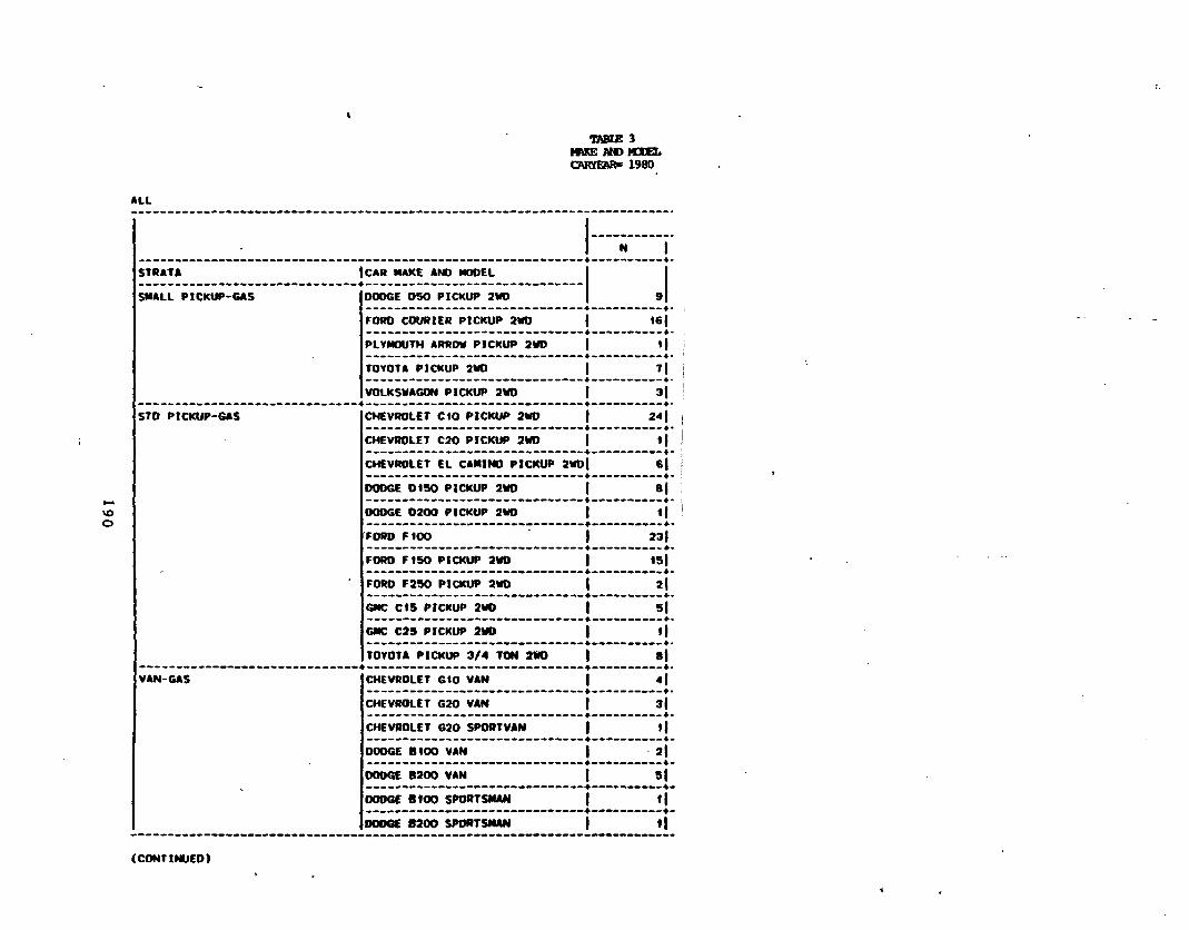
TRBtB 3WKEMOHXELCAIOEftR- 1980
ALL
VOO
STRATA |CAR MAKE AND MODEL
SMALL PICKUP-GAS
STD PICKUP-GAS
VAN-GAS
DODGE D5O PICKUP 2ND
FORD COURIER PICKUP 2W0
PLYMOUTH ARROW PICKUP 2WD
TOYOTA PICKUP 2WD
VOLKSWAGON PICKUP 2V0
CHEVROLET CIO PICKUP 2W0
CHEVROLET C20 PICKUP 2W0
N
9
1 «M»l7|
3|
1 24|
'1CHEVROLET EL CAMINO PICKUP 2W0| 6|
DODGE D1S0 PICKUP 2W0
DODGE O2OO PICKUP 2HD
FORD F100
FORD F15O PICKUP 2WD
FORD F250 PICKUP 2WD
GMC CIS PICKUP 2WO
GMC C25 PICKUP 2WO
TOYOTA PICKUP 3/4 TON 2WD
CHEVROLET GtO VAN
CHEVROLET G20 VAN
CHEVROLET G20 SPORTVAN
DODGE 8100 VAN
DODGE 8200 VAN
DODGE 8100 SPORTSMAN
DODGE 8200 SPORTSMAN
8|
1 '11 231
1S|
i 2 |
1 s|1 *l1 8|
1 4|
1 3|
1 '11 ' 2|
| 1|
(CONTINUED)

TABUS 3MAKE N © K E E LCMWERR= 1 9 8 0
ALL
STRATA
VAN-GAS
SPtClAL USE-GAS
SMALL PICKUP 4W0
STD PICKUP 4M0
SPECIAL USE 4WO
CAR MAKE AND MODEL
DODGE B3OO SPORTSMAN
FORO E 100 CLUB WAGON
FORO E ISO CLUB WAGON
GMC G2S VAN
PLYMOUTH PB1OO VOYAGER
VOLKSWAGON VANAGON
CHEVROLET CIO BLAZER
CHEVROLET CIO SUBURBAN
CHEVROLET C2O SUBURBAN
CHEVROLET LUV
TOYOTA PICKUP
CHEVROLET K-1O
CHEVROLET K-20
DODGE DtSO
DODGE W2OO
FORO F15O
FORO F25O
GMC K15
JEEP J10
CHEVROLET K10 BLAZER
CHEVROLET KtO SUBURBAN
DODGE AW100 RAMCHARGER
FORO BRONCO
111
11111111111111111111111
N I
2
4|
«4|
1
M
U2|
1
2O|
241
15|
"12|
H241
11|
4
2|
4|
1|
2|
19|
(CONTINUED)

3M1980
ALL
STRATA
SPECIAL USE 4W0
SML PKUP DIE 2WJ
SID PKUP DIE 2ND
-_-•._-«—..——•__,»•«»«_••«<»•_..——•.—_.•_—..—_.••..•__..—_—...•.—.._—«_.._——•..*+».—«—«-»...•_«.
| CAR MAKE AND MOOEL
GMC K1S JIMMY
GMC K1S SUBURBAN
JEEP CHEROKEE
JEEP CJ-S
JEEP CJ-7-.-—-.------_._---_-.-—----.«--—_..-__JEEP tfAGONEER
PLYMOUTH PW1OO TRAIL OUSTER
|VOLKSWAGON
3|-•
1|
to ICHEVROLET C-IOGMC CIS

•raaue 3MAKE MID MXEt.
1981
ALL
voCO
STRATA
MINI
SUB-COMPACT
CAR MAKE AND MODEL
CHEVROLET CORVETTE (2-SEATER)
DATSUN 28OZX (2-SEATER)
HONDA CIVIC
HONDA PRELUDE
TOYOTA STARLET
N
3
5
46
2O
12
AMC EAGLE | 1
AMC EAGLE KAMMBACK SX4
AMC SPIRIT
3
7
CHEVROLET CAMARO | 12
CHEVROLET CHEVETTE
DATSUN 2OOSX
1O5
10
DATSUN 21O | 29
DATSUN 28OZX 2*2
DATSUN 3 to
DATSUN S1O
2
6
5
OATSUN 810 | 1
DODGE CHALLENGER
DODGE COLT
DODGE O24
FORD MUSTANG
HONDA ACCORD
LINCOLN-MERCURY CAPRI
2
B
21
S2
PLYMOUTH CHAMP | 1O

TABIB 3HAKE MID MODELCATOEftR" 1 9 8 1
ALL
vO
STRATA
SUB-COMPACT
•
CAR MAKE AND MODEL
PLYMOUTH SAPPORO
PLYMOUTH TC3
PONTIAC FIREBIRD
TOYOTA CELICA
TOYOTA CELICA SUPRA
TOYOTA COROLLA
TOYOTA COROLLA TERCEL
TOYOTA CORONA
TOYOTA CRESSIOA
VOLKSWAGON RABBIT
VOLKSWAGON SCIROCCO
111111111111
6
1G|
G|
35|
2|
661
43|
6
8|
•1H
COMPACT
MIDSIZE
AMC CONCORD
BUICK SKYLARK
DODGE OMNI
FORD ESCORT
LINCOLN-MERCURY LYNX
OLDSMOBILE OMEGA
PLYMOUTH HORIZON
BUICK CENTURY
BUICK REGAL
BUICK RIVIERA
CAOILLAC ELDORADO
CADILLAC SEVILLE
11I1|I
|111
2|
«3|
321
321
3S|
4|
a|
(CONTINUED)

AND MODELCMOfEftft. 1981
ALL
vx>
STRATA
MIDSIZE
CAR MAKE AND MODEL
CHEVROLET CITATION
N I
77
CHEVROLET MALIBU | 19|
CHEVROLET MONTE CARLO
CHRYSLER CORDOBA
CHRYSLER IMPERIAL
CHRYSLER LEBARON
291
4|
2|
«lDODGE ARIES | 31|
DODGE OIPLOMAT | i|
DODGE MIRADA
FORD FAIRMONT
FORD GRANADA
FORD THUNDERSIRD
LINCOLN-MERCURY COUGAR
LINCOLN-MERCURY XR7
LINCOLN-MERCURY ZEPHYR
OLDSMOBILE CUTLASS
OLOSMOBILE CUTLASS CALAIS
OLDSMOBILE CUTLASS SALON
OLOSMOBILE CUTLASS SUPREME
PLYMOUTH RELIANT
PONTIAC GRAND PRIX
PONTtAC LEMANS
PONTIAC PHOENIX
*l19|
19|
«l1|
3|
5|
22|
el"I41|
341
371
1O|
371
(CONTINUED)

CDELCMttEAR= 1981
ALL
STRATA
LARGE
|CAR MAKE AND MODEL
BUICK ELECTRA
BUICK LESA8RE
CADILLAC DEVILLE
CADILLAC FLEETWOOD
CHEVROLET CAPRICE
CHEVROLET IMPALA
CHRYSLER NEWPORT
CHRYSLER NEW YORKER
FORD LTD
LINCOLN-MERCURY MARQUIS
OLOSMOBILE DELTA 88
OLDSMOBILE NINETY-EIGHT
PONT I AC BONNE V R L E
PONTIAC CATALINA
LINCOLN MARK VI
11111i11111111
io|
t|
1*1
s|i|
1|
7|
8|
" |
«l13|
1|
5|
LINCOLN CONTINENTAL TOWN ftCOUNTRY .ol
SMALL STN WAGON AMC EAGLE WAGON
AMC CONCORD WAGON
OATSUN 21O WAGON
OATSUN 51O WAGON
OATSUN 81O WAGON
HONDA CIVIC WAGON
S|
"aij"
(CONTINUED)

TABLE 3JWDHDDEL
CRBYERR. 1 9 8 1
ALL
vo
STRATA
SMALL STN WAGON
MIDSIZE WAGON
LARGE WAGON
CAR MAKE AND MODEL
TOYOTA COROLLA WAGON
TOYOTA CORONA WAGON
TOYOTA CRESSIDA WAGON
BUICK CENTURY WAGON
CHEVROLET MALIBU WAGON
CHRYSLER LEBARON WAGON
DODGE ARIES WAGON
FORD FAIRMONT WAGON
LINCOLN-MERCURY ZEPHYR WAGON
OLDSMOBILE CUTLASS WAGON
PLYMOUTH RELIANT WAGON
N I
361
5|
2|
21|
2|
381
ia|
t|
101
«lPONTIAC LEMANS SAFARI WAGON | 1O|
CHEVROLET CAPRICE 4|
CHEVROLET IMPALA | 6|
BUICK ELECTRA ESTATE WAGON | 1|
FORD LTD WAGON «lLINCOLN-MERCURY MARQUIS WAGON | 3|
OLDSMOBILE CUSTOM CRUISER I IWAGON I 31
PONTIAC BONNEVILLE SAFARI 1 1WAGON 1 _|
SUBCOMPACT DIES |VOLKSWAGON RABBIT | 741
MIDSIZE DIESEL CADILLAC ELDORADO | 3|
OLDSMOBILE CUTLASS ail
(CONTINUED)

MAKE ANDHXEt.C7VFKERR. 1981
ALL
00
STRATA |CAR MAKE AND MODEL
MIDSIZE DIESEL
LARGE DIESEL
SMALL WAGON-DIES
MID WAGON-DIES
LG WAGON-DIES
SMALL PICKUP-GAS
OLDSMOBILE CUTLASS CALAIS
OLDSMOBILE CUTLASS SUPREME
PONTIAC GRAND PRIX
OLDSMOBILE TORONAOO
BUICK ELECTRA
BUtCK LESABRE
CADILLAC DEVILLE
CADILLAC FLEETWOOD
CHEVROLET CAPRICE
CHEVROLET IMPALA
PONTIAC BONNEVtLLE
OLDSMOBILE 88
OLDSMOBILE 98
VOLKSWAGON DASHER
OLDSMOBILE CUTLASS CRUISERWAGON
BUICK ELECTRA ESTATE WAGON
OLOSMOBILE CUSTOM CRUISERWAGON
CHEVROLET CAPRICE WAGON
PONTIAC BONNEVILLE WAGON
CHEVROLET LUV PICKUP
DATSUN PICKUP
DODGE RAMSO PICKUP
M 1" 1
1el341
61
4|
3|
ail
"II 2|
1 «l
1 2O|
(CONTINUED)

3
1981
ALL
STRATA
SMALL PICKUP-GAS
|CAR MAKE AND MOOEL
FOOD COURIER PICKUP
PLYMOUTH ARROW PICKUP
TOYOTA TRUCK
VOLKSWAGON PICKUP
1|
121
STD PICKUP-GAS CHEVROLET CIO PICKUP
CHEVROLET C2O PICKUP
CHEVROLET EL CAMINO PICKUP
DOOGE O1SO PICKUP
DODGE D25O PICKUP
FORO F1OO
FORD F1SO PICKUP
FORD F2SO PtCKUP
GMC C49 PICKUP
GMC C2S PICKUP
TOYOTA PtCKUP 3/4 TON
CHEVROLET G2O VAN
<M
H26|
VAN-GAS
CHEVROLET G1O SPORTVAN
CHEVROLET G2O SPORTVAN
DOOGE B15O VAN
DODGE B2SO VAN
DODGE B«5O SPORTVAN
DODGE 8230 SPORTSMAN
FORO E10O ECONOLINE
I-•-
I-•-
I
21
31
(CONTINUED)

TRBI£ 3E AND MOtEL
1981
ALL
oo
STRATA
VAN-GAS
SPECIAL USE-GAS
SMALL PICKUP 4MD
STD PICKUP 4WD
CAR MAKE AND MODEL
FORD E15O ECONOLINE
FORD E25O ECONOLINE
GMC G15 VAN
GMC G2S VAN
GMC G25 SPORTVAN .
PLYMOUTH PB15O VOYAGER
VOLKSWAGON VANAGON
CHEVROLET CIO BLAZER
CHEVROLET CIO SUBURBAN
CHEVROLET C2O SUBURBAN
GMC C15 SUBURBAN
CHEVROLET LUV
DATSUN
TOYOTA PICKUP
CHEVROLET K-1O
CHEVROLET K-2O
DODGE W15O
DODGE W2SO
FORD F150
FORO F25O
N I
•1
2|
3|
1|
a|4|
3|
4|
1 H
s|1 "1
23|
1|
4O|
1 f\GMC K1S | 1|
GMC K25
JEEP «I1O
«lal
(CONTINUED)

TABIE 3AND HXEL
1981
ALL
STRATA
STO PICKUP 4WD
|CAR MAKE AND HOOEL
|JEEP 020
to
SPECIAL USE 4W0 CHEVROLET K1O BLAZER
DODGE AV1OO RAMCHARGER
FORD BRONCO
GMC K15 SUBURBAN
JEEP CJ-5
JEEP CJ-7
JEEP CJ-B (SCRAMBLER)
JEEP WAGONEER
TOYOTA LAND CRUISER WAGON
111111111
7I3|
13|
3|
5|
H"sal"45l
SML PKUP DIE 2WD ITOYOTA
IVOLKSWAGON
STO PKUP OIE 2WD ICHEVROLET C-1OGMC CIS

APPENDIX B
ESTIMATION OF AVERAGE VEHICLE AGE
202

Month (Yr)
October '76
November '76
December '76
January '77
February '77
March '77
April '77
May '77
June '77
July '77
August '77
September '77
October '77
November '77
December '77
VehicleSales'*
730,216
720,772
694,457
601,325
665,978
895,319
B21.969
833,333
919,142
731,033
726,422
656,600
869,920
737,362
645,991
ESTIMATION OF AVERAGEFROM
VEHICLE SALES
Proportion ofMonthly SalesAssumed to BeModel Yr 1977
2/3
3/4
ALL
•t
n
•i
n
n
ii
•I
• «i
II
1/3
1/4
None
VEHICLE AGE
DATA
S Salesby Month,Model Yr1977
5.36
6.40
7.64
6.62
7.33
9.85
9.04
9.17
10.11
8.04
7.99
7.23
3.19
2.03
0
AverageVehicle Age,in months
as of1 July 1978
20.5
19.5
18.5
17.5
16.5
15.5
14.5
13.5
12.5
11.5
10.5
9.5
8.5
7.5
Source: a - Automotive News, various weekly publications for 1976 - 1978.
203
The average vehicle age for the 1977 Model Year fleet, as of 1 Duly 1978,is computed from the above table by taking the sales-weighted average ofthe individual monthly ages of the vehicles (e.g., the sum of the productsof the numbers in columns 4 and 5 of the table). This number turns out tobe:
14.34 months = 1.195 years
or approximately 1.2 years.
Thus on 1 Duly 1983, the midpoint of the 1983 On-Road Survey, Model Year1977 vehicles would be approximately 1.2 • 5 or 6.2 years old.
Note in column 3 of the table that all vehicle sales from December 1976through September 1977 are considered to be 1977 Model Year vintage,whereas only portions of the sales for months October and November 1976,and October and November 1977 are considered to be Model Year 1977vehicles. This is done to account for the sale of carry-over model yearvehicles into the beginning of the subsequent model year.
The year 1977 has been assumed as typical insofar as portraying thedistribution of vehicle sales by month, and hence the computation ofaverage vehicle age, as used in Chapter 3 of the report.
20A

APPENDIX C
SURVEY SUPPORT MATERIALS
205

O.H.B. No. 2127-0037Explra* 9/30/84
US Department 400 s**nth St., s.w.Of TtanspOftatiOn Washington, D.C. 20590
NcrHoool HJflhwoyltofflc SafetyAdmW8tratten PRENOTtFICA TION
LETTER ~ NHTSA
Dear Driver:
We need your help . . .
Your name has been selected at random from among all owners oflate model cars and light trucks to participate 1n a nationwidesurvey.
The National Highway Traffic Safety Administration, an Agency ofthe U.S. Department of Transportation, 1s sponsoring the surveyto measure the gas mileage performance of late model vehicles.Information obtained 1n the survey will tell us how much the Nation1s saving as a result of the more fuel-efficient vehicles produced1n the last few years, and will help determine future directions1n energy conservation efforts.
The National Opinion Research Center, an experienced survey firm,will conduct the study for us. Within the next few days, theywill be sending you a copy of a simple fuel-mileage log. Completionof the log will require only a few minutes of your time; TheInformation, of course, will be vital to our study but we believeyou will find 1t personally useful as well.
We want to assure you that while your participation 1n this survey1s entirely voluntary, your response 1s very Important to ensurethe accuracy of the results. The survey complies with all Federalregulations concerning privacy and confidentiality and the resultswill be used only 1n statistical summaries.
We look forward to your cooperation In this Important undertaking.
Sincerely,
ZL,Barry FelriceAssoc1ateAdm1n1strator for
Plans /nd Programs
206

J/JO/M
tear
I f you are l ike most of us, you have become very aware of the high cost ofgasoline 1n today's family budget. "M11es-per-gal1on" Is the f i r s t thingmost of us think of when we shop for a new or used car or truck.
In order to meet the problems of fuel conservation and cost, automobilecompanies have been manufacturing smaller and l ighter vehicles 1n recentyears.
We have been asked by the National Highway Traff ic Safety Administration(see le t ter enclosed] to find out just how ef f ic ient these new vehicleshave become. To do t h i s , we are conducting a nationwide survey of vehicleowners l ike yourself who have purchased these late models.
How can you help us? By keeping a simple record of your gas purchases overthe next month for the vehicle l isted below.
In a few days, we wi l l send you a small fuel-mileage log. Completion of thelog wi l l take only a few minutes of your time. In the event you no longerown the vehicle, or wi l l not be operating I t next month, please detach theform below and return 1t to us as soon as possible.
We look forward to your participation In this Important study.
Sincerely,
Jean AttuJean AtkinsonSenior Survey Director
Conducted by: NUIonal Opinion feMircnConMr • tMO South till* • CMcago. 1110637UnWnltyolCnlMQO
! PLEAVEDETACH THIS FOnM'AMDHlwnNmTHBPoifAQYiMDyNvYLO
1 VIHICU: HAKE MODEL YIAW I I I I 1 I I I
I to «M* talk** |mM t
I :Tft*NhMtlMitMMM I | | N«IOlM|lMtomiMMiri*««ft*«»«nan»wliMilii
BipCod»)_
207

O.H.B. No. 2127-0037Enplrtt 9/30/84
USDepartment - • 400 8 M » * st., s.w.of TrnnsDortotion WMhmgton. DC. 20590
National Highway
ON TH€ RORD FU€L €COHOMV SURV6V
QU£STIONNAIR£ TRANSMITTAL LETTERDear Driver: /7/?57 W4V£" "~A few days ago we wrote that you had been chosen to participate 1n anational On The Road Fuel Economy Survey.
Enclosed 1s a Fuel Mileage Log and two decais for this U.S. Department ofTransportation study. The Log should be kept 1n some convenient spot Insideyour vehicle next month for ready access at "fill-up" time. One of thedecals can be placed on the dash near the fuel gauge, as a reminder to you,or anyone else who drives, to record each gas purchase for the month. Thedecal can be easily removed after the survey, and will leave no residue onyour vehicle.
Before placing the Log 1n your vehicle, please complete the description ofyour vehicle In Section A. Then, each time you buy gas next month, simply fill1n one line of Section B, the Gas Mileage Log.
Please try to fill the tank completely, at least for the first and lastpurchases of the month, to enable us to make good estimates of your mileage.
At the end of the month, please return the Log to us. Simply fold the Log asIndicated, seal with (second) decal or tape, and drop 1t In the mall. Nopostage 1s needed.
Because we believe you may find a record of your fuel mileage personallyuseful, we have enclosed a handy booklet which you may keep for yourself.You may also find the booklet a convenient place to keep the Log during thesurvey month.
The Information you supply will be an Important aid 1n determining futureenergy needs of our country, and we are looking forward to your participation1n our study.
Thank you for your help.
Sincerely,
Jean AtkinsonSenior Survey Director
Enclosures
Conducted t>y *'*t'on*l Opinion Rwsejfch Center • 6030 South E'lis • Chicago, IL 60837l C ••„:>
208


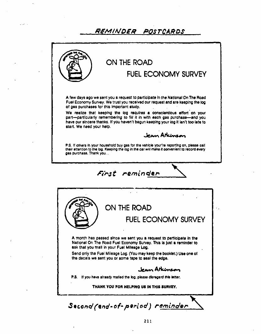
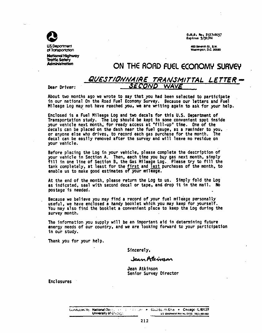
O.M.B. No. 2127^-0037Explrtt 5/30/8*
U S Deportment 400 swmtn si., s.w.of Transportation wainmgton, D,C. 20500
National Highwaytattle Safety
Administration r\M TU£ RQRD FU€L 6COROMV SURV€V
TRANSMITTAL LETTER -Dear Driver: SECOND WAVEAbout two months ago we wrote to say that you had been selected to participatein our national On the Road Fuel Economy Survey. Because our letters and FuelMileage Log may not have reached you* we are writing again to ask for your help.
Enclosed 1s a Fuel Mileage Log and two decals for this U.S. Department ofTransportation study. The Log should be kept 1n some convenient spot Insideyour vehicle next month, for ready access at "f1ll-up" time. One of thedecals can be placed on the dash near the fuel gauge, as a reminder to you,or anyone else who drives, to record each gas purchase for the month. Thedecal can be easily removed after the survey and will leave no residue onyour vehicle.
Before placing the Log in your vehicle, please complete the description ofyour vehicle in Section A. Then, each time you buy gas next month, simplyfill in one line of Section B, the Gas Mileage Log. Please try to fill thetank completely, at least for the first and last purchases of the month, toenable us to make good estimates of your mileage.
At the end of the month, please return the Log to us. Simply fold the Logas Indicated, seal with second decal or tape, and drop 1t in the mall. Nopostage 1s needed.
Because we believe you may find a record of your fuel mileage personallyuseful, we have enclosed a handy booklet which you may keep for yourself.You may also find the booklet a convenient place to keep the Log during thesurvey month.
The Information you supply will be an important aid in determining futureenergy needs of our country, and we are looking forward to your participationIn our study.
Thank you for your help.
Sincerely,
Jean AtkinsonSenior Survey Director
Enclosures
National Oe> •... •• ; • : • ..'•• • &'jijfec.*fitn.s • CmctgcH.ttoe37University of Cue;-;,•. us wwmiw mvm:. cwci
212

TELEPHONE Qt/ES TIQNNAIREFORM APPROVED THRU 9/ jO/B*O.H.B. NO. 2127-0037
ON THE ROAD NONRESPONSE FOLLOVUP
TELEPHONE QUESTIONNAIRE
THE SALUTATION AND CLOSING OF THE INTERVIEWER'S MESSAGE WILL BE AS FOLLOWS:
Salutation - "Hello (name). This is (INTERVIEWER'S NAME) from the NationalOpinion Research Center of the University of Chicago. I as calling to checkwhether you received any of the letters we have sent to you In the pastsonth(s) about the national On The Road Survey we are conducting for theDepartment of Transportation." (On to Questionnaire Item 1)
IF RESPONDENT VOLUNTEERS THAT HE OR SHE HAS RECEIVED NO INFORMATIONINTERVIEWER WILL EXPLAIN, "We have been asked by the National Highway TrafficAdministration to find out just how efficient new vehicles have become inmiles per gallon for the average motorist. To do this, we are conducting anationwide survey of late model vehicles* and we understand that you ownone.* (On to Questionnaire Item 2)
Closing - IF THE RESPONDENT IS RELUCTANT TO PARTICIPATE THE CALL WILL BEPOLITELY TERMINATED WITH THE INTERVIEWER EXPRESSING GRATITUDE FOR HIS OR HERCOOPERATION IN RECEIVING THE CALL.
- IF THE RESPONDENT AGREES TO ACCEPT LOG THE INTERVIEWER WILL SAY
"Thank you for agreeing to help us in this survey, the informationyou supply will be an important aid in the development of more fuel*efficient vehicles in this country*
Within a few days you will receive a fuel mileage log and acomplimentary booklet from the Department of Transportation.Recording your gas purchases will be simple if you keep the log Inyour vehicle. Thank you again."
213

Phan* yuisiiohrAJr* - -2-
Telephone Interview
(See introduction page)
1. Did you receive any of our recent letters about this survey?
No I 2
2. Have you ever owned(READ Label Below)
Make:
IF YES
Do you
Model: Year:
TO 2:
still own this vehicle?
What became of the vehicle?It was
It was
Other
Yes
No
Yes
No
sold
junked
specify*
CD1—I
1—1(—i
I—ii—iI—i
i
2
1
2
1
2
3
ASK 3
GO TO 5B ANDEND
ASK
ASK
ASK
INTERVIEW
6
4
5
5. A. Do you have the name and address of the person to whom it was sold?
(Name)
(Address)
(Town) (Zip)
B. THANK RESPONDENT AND TERMINATE INTERVIEW IF RESPONDENT NO LONGER OWNSCAR.
•INTERVIEWER INSTRUCTION—CONTINUE INTERVIEW IF CAR IS STILL OWNED/USED BYPERSON(S) IN RESPONDENT'S HOUSEHOLD.
214

PhonQ qaBstlonn&tre - -3-
6. He are trying to Improve our survey procedures and I would like to askyou a few questions about why you were unable to participate in the Onthe Road Survey* This should take only a few minutes of your tine.
why were you unable to complete the fuel mileage log?
Did not drive the vehicle .......
Did not wish to participate »••••
Too busy ..««....«.««««««..«.<«•.
Object to surveys(Probe "Why is that?")
Did not understand about thesurvey or task (Probe:"What was it you didn'tunderstand?")
Other reason (SPECIFY)
1 ASK 7
2'
3
ASK 8
7. Is the car now back on the road?
Yes
No
1 I 1 GO TO 8
2 GO TO 5B ENDINTERVIEW
8. I have a few questions about your vehicle.
INTERVIEWER COMPLETE FACSIMILE OF CAR MILEAGE LOG NEXT PAGE AND CHECKBELOW.
Section A & B completed I 1 1Not completed (give reason) ... 1 I 2
215
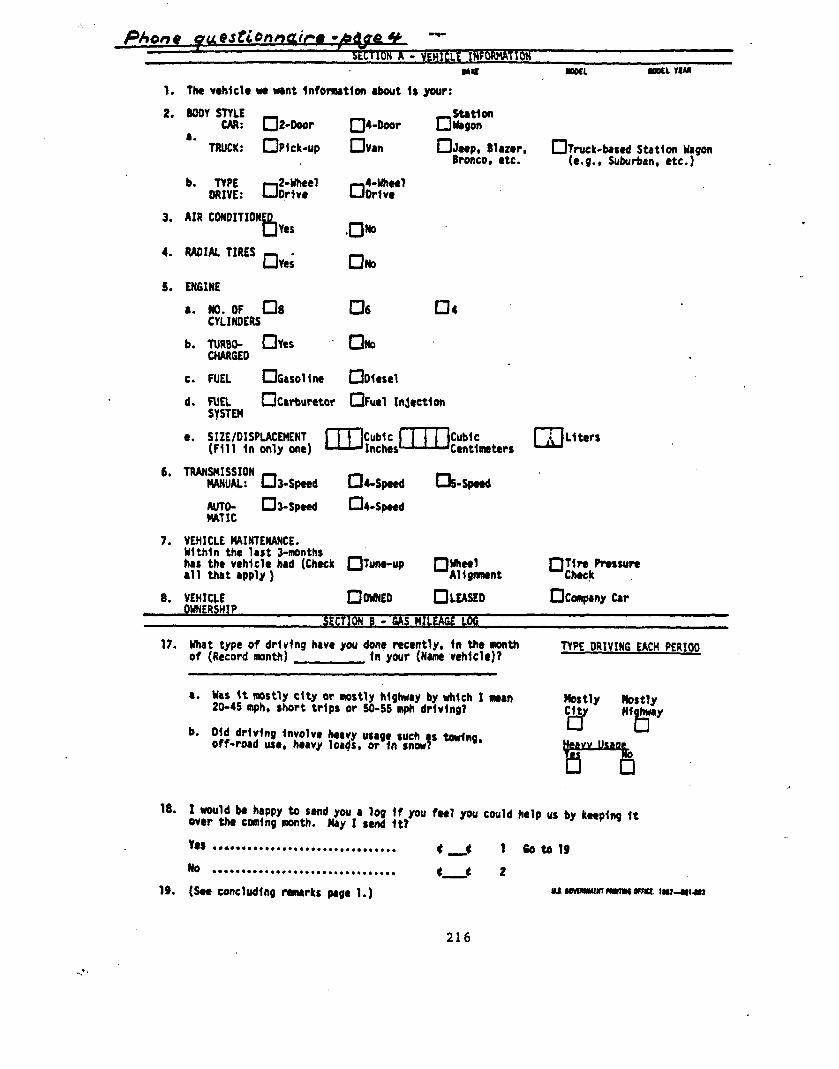
PAoot? questionnaire5ECTHW A - VEHICLE IWrOwnATIOH
MtC
1. The vehicle we want Information about 1s your:
2.
3.
4.
S.
BODY STYLECAR:
a .TRUCK:
b. TYPEDRIVE:
AIR CONDITI
D2-0oor
OP1ck-up
1-,2-WheelLJDrive
ONED
RADIAL TIRES —. ••Yes
ENGINE
a. NO. OF D aCYLINDERS
b. TURBO-CHARGEO
c. FUEL
d. FUELSYSTEM
DY«
OGasoline
Ocarburetor
•4-0oor
Dvan
,-,4-WheelLJOrivc
DNO
De
DNO
Ddesel
—StationDragon
Djeep, BBronco,
D4
DFUCI Injection
e. SIZE/DISPLACEMENT I I \ jCubic I 1 I I ICubic( F i l l 1n only one) • •' ^ I n c h e s ' 1 '• ' L JCent1weters
Ds-Spttd6. TRANSMISSION _ _ .
MANUAL: U 3-Speed U 4 - S p e e d
AUTO- D3-Spee<t D4-SpeedMAT1C
7 . VEHICLE MAINTENANCE.Within the last 3-months mm'has the vehicle had (Check MTune-upall that apply )
8. VEHICLEOWNERSHIP
DOWNEDAlignment
DLEASED
•ML HKL T(M
DTruck-based Station Wagon(e.g.. Suburban, etc.)
Liters
•T1re PressureCheck
Dcompany Car
SECTION B - SAS MILEAGE LOG
17. What type of driving have you done recently, 1n the monthof (Record month) In your (Name vehicle)?
TYPE DRIVING EACH PERIOD
a. Was 1t mostly dty or mostly highway by which I mean20-45 mph, short trips or 50-55 moh driving?
b. Old driving Involve heavy usage such as towing,off-road use, heavy loads, or In snow? w " i n B »
Mostly MostlyCity Highway
ivv Usage
Yes
Mo
19. (See concluding remarks page 1.)
t t 1 6o to 19
t t 2
216

O.N.B. No. 2127-0037Explr** 3/30/84
US Department 400 swtnth St., s.w.of lansponation wuhtyton, DJC. 20500
National M g h w a yTtwfflc Sofsty
ON TH€ RORD FU€L €COnOMV SURV€VGLi/ZSTIONNAlRE TRANSM1TTAL LETTER-
Dear Driver:
Thank you for agreeing to participate 1n our Important survey of OnThe Road Fuel Economy.
Enclosed Is a Fuel Mileage Log and two decals for this U.S. Departmentof Transportation study. The Log should be kept 1n some convenient spotInside your vehicle next month, for ready access at "fill-up" time. Oneof the decals can be placed on the dash near the fuel gauge, as areminder to you, or anyone else who drives, to record each gas purchasefor the month. The decal can be easily removed after the survey and willleave no residue on your vehicle.
Before placing the Log 1n your vehicle, please complete the descriptionof your vehicle 1n Section A. Then, each time you buy gas next month,simply fill in one line of Section B, the Gas Mileage Log. Please tryto fill the tank completely, at least for the first and last purchasesof the month, to enable us to make good estimates of your mileage.
At the end of the month, please return the Log to us. Simply fold theLog as Indicated, seal with second decal or tape, and drop 1t in themall. No postage 1s needed.
Because we believe you may find a record of your fuel mileage personallyuseful, we have enclosed a handy booklet which you may keep for yourself.You may also find the booklet a convenient place to keep the Log duringthe survey month.
The Information you supply will be an Important aid 1n determining futureenergy needs of our country, and we are looking forward to yourparticipation in our study.
Thank you for your help.
Sincerely,
Jean AtkinsonSenior Survey Director
Enclosures
National Opinion ..»«,en i^mer • fc&Sb*'inUti» • Covcaeo, I t 60637Unlyrttty of Chicago
217

APPENDIX D
METHODOLOGY AND DATA FOR ESTIMATING REDUCED ENERGYCONSUMPTION AND EQUIVALENT DOLLAR VALUE
218

ANNUAL AND LIFETIME MILEAGE ESTIMATES, AVERAGE PASSENGER CARAND LIGHT TRUCK
In order to estimate total lifetime reduction in energy
consumption and dollar equivalent values for the vehicles studied in the
On-the-Road Fuel Economy Survey, it is necessary to have an estimate of the
total miles that an average vehicle will travel in its lifetime and also an
estimate of how this mileage is distributed by the age of the vehicle.
In Chapter 3, Table 3-10, estimates were developed for the average
vehicle miles per vehicle age for the U.S. population of privately^ owned
passenger cars and light trucks. These estimates constitute the principal
basis for estimating lifetime and yearly miles traveled for the average
vehicle. Two adjustments must be made to these data, however, before they
can be used to estimate total lifetime reductions in energy consumption and
dollar equivalent values.
First, an adjustment must be made to account for the miles driven
by fleet vehicles, which were not sampled in the survey. Fleet vehicles are
known to be newer, in general, and also to be driven, on a per vehicle
basis, more miles annually than the average vehicle in the U.S. population.
Secondly, the miles per year data in Table 3-10 represent travel by vehicles
which are still on the road at age x. In order to get miles per year for
1 The ORFES sampling frame included only vehicles owned and operated byprivate individuals. Fleet vehicles such as business fleets, rental fleets,police fleets, taxi fleets, government fleets, etc., were not sampled due tothe operational constraints of collecting reliable data on these vehicles,as explained in the report.
219

the average vehicle in the U.S. population, these numbers must be
multiplied by the probability than a given vehicle will still be on the
road, or survive to, age x.
Tables D-1 and D-2 contain the vehicle travel data adjusted as
described above, that were used to develop the estimates of energy reduction
and dollar equivalent values in this report, for cars and trucks,
respectively. The second columns of each table are a reproduction of the
last column of Table 3-10 from Chapter 3 with the following two exceptions:
(1) Rows 1-6 of Table D-1 have been revised to incorporate
annual travel by fleet vehicles. The bases for these
estimates are that fleet vehicles number about 10,000,0002,3
travel an average of 24,000 miles per vehicle, per year; and
have a total life-span of approximately six years.A
2 "Transportation Energy Data Book," Edition 7, Op. Cit.3 "Characteristics of Automotive Fleets in the United States, Shonka, Op. Cit,4 Shonka, Op. Cit., gives 2.5 years as the average age of fleet cars at the
time they are resold. Since some vehicles will be replaced earlier thanthis, and some later, 6 years is taken as the maximum time a fleet car willremain in a fleet status.
220

TABLE D-1
ESTIMATED VEHICLE MILES, LIFETIME PASSENGER CARS
VehicleAgeYears
123456789
1011121314151617181920
VehicleMilesTraveled!./
15,700• 14,040
13,55011,0289,4688,4834,4853,8853,4273,0662,7732,5322,3292,1562,0071,8781,7641,6631,5731,493
VehicleSurvivalProbability**/
1.000.993.982.964.935.892.831.753.662.568.476.394.323.263.213.172.139.112.090.073
Vehicle MilesTraveled, Lifetime,Average Vehicle
15,70013,94213,30610,6318,8537,5673,7272,9252,2691,7411 ,320
998752567427323245186142109
TOTAL 85,730
—/ From Table 3-10 of Chapter 3, adjusted to incorporate fleet vehicletravel, as described in accompanying text.
b/ Source: "Scrappage and Survival Rates of Passenger Cars and Trucks in1970-1982 ," P. Hu", Transportation Energy Group, Oak Ridge NationalLaboratory, August 10, 1983.
221
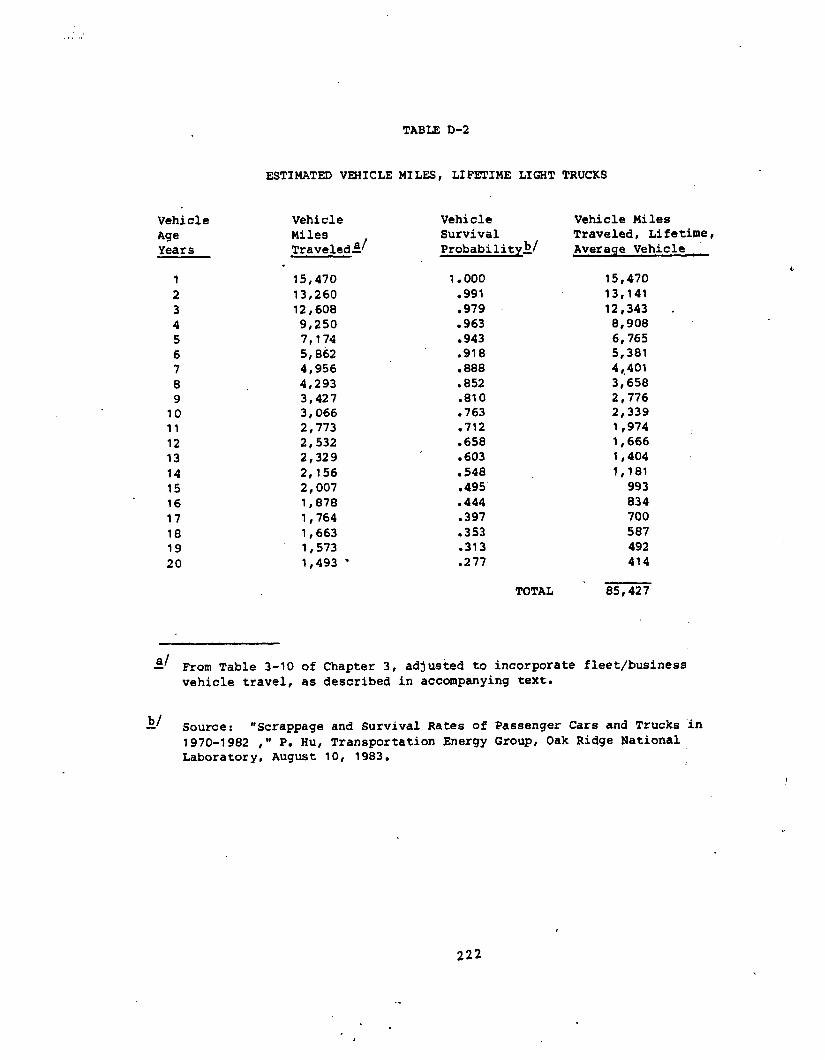
TABLE D-2
ESTIMATED VEHICLE MILES, LIFETIME LIGHT TRUCKS
VehicleAgeYears
123456789
1011121314151617181920
VehicleMilesTraveled^'
15,47013,26012,6089,2507,1745,8624,9564,2933,4273,0662,7732,5322,3292,1562,0071,8781,7641,6631,5731,493 *
VehicleSurvivalProbability*5/
1.000.991.979.963.943.918.888.852.810.763.712.658.603.548.495.444.397.353.313.277
Vehicle MilesTraveled, Lifetime,Average Vehicle
15,47013,14112,3438,9086,7655,3814,4013,6582,7762,3391,9741,6661,4041,181
993834700587492414
TOTAL 85,427
— From Table 3-10 of Chapter 3, adjusted to incorporate fleet/businessvehicle travel, as described in accompanying text.
— Source: "Scrappage and Survival Rates of Passenger Cars and Trucks in1970-1982 ," P. Hu, Transportation Energy Group, Oak Ridge NationalLaboratory, August 10, 1983.
222

(2) Rows 1-8 of Table D-2 have been revised to incorporate annual
travel for light trucks operating in a fleet environment or
read for business purposes. The bases for these estimates
are that fleet/business5 trucks represent approximately
one-half of the total light truck population6; travel
approximately 21 percent more miles annually, than
private-use trucks, and have a total lifespan of
approximately 8 years.'
The third columns of Tables D-1 and 0-2 contain the vehicle
survival probability estimates.^ The last column of each table is the
estimated yearly travel for the average vehicle and is merely the product of
the annual miles traveled (column 2) and the probability that the vehicle
will survive to age x (column 3). The sum of column 4 represents the
estimated total lifetime travel for the average vehicle, 85,730 miles, and
85,427 miles, for cars and trucks respectively.
5 49.1 percent of total pickup trucks are classified as having vehicle andoperational characteristics other than for personal transportation (i.e.,mining, construction, utilities, etc.) Sources: 1972 Census ofTransportation, Volume II, Truck Inventory and Use Survey, U.S. Departmentof Commerce, issued March 1974; "Projection of Light Truck Population Year2025," Oak Ridge National Laboratory, ORNL/Sub-78/14285/1 Special, October1978.
6 Average annual mileage for pickup trucks used for fleet business purpose= 11,945 versus 9,900 for pickup trucks used for personal transportation((11,945-9,90O)/9,900 = 21 percent). Source: 1972 Census ofTransportation, Op. Cit.
7 Available data on survival rates show trucks to have a somewhat longerlifespan than cars; hence 8 years is taken as the maximum time a truck willremain in a fleet/business status. Source: "Scrappage and Survival Ratesin Passenger Cars and Truck in 1970-1972, P. Hu, Transportation EnergyGroup, Oak Ridge National Laboratory, August 10, 1983.
8 "Scrappage and Survival Rates in Passenger Cars and Trucks in 1970-1982,"Op. Cit.
223

FUEL REDUCTION ESTIMATES
In order to estimate per vehicle lifetime reduction in fuel use
for a given model year, say 1978 passenger cars, it is merely necessary to
take the product of the total estimated lifetime mileage (from column 4,
Table D-1) and the per vehicle reduction in fuel use, in gallons of fuel per
mile driven versus the 1977 models (as computed in Chapter 2). For total
model year reduction (i.e., all vehicles sold), the per vehicle reduction is
simply multiplied by the total number of vehicles sold in the given model
year.
EQUIVALENT DOLLAR VALUE OF REDUCTION IN ENERGY USE
In order to estimate dollar equivalent value of the reduced fuel
consumption, it is necessary to have estimates of the cost of gasoline in
addition to the estimates of vehicle miles traveled and the per vehicle
reduction in fuel consumption in fuel per unit of travel for the study
vehicle over the baseline vehicle.
Since annual vehicle travel varies with vehicle age (specifically,
the survey data from Chapter 3 shows a distinct decline in the rate of
travel as vehicle age increases, with a large proportion of total lifetime
travel occurring in the early years of vehicle life), and since the real
price of gasoline is projected to increase over time, it is therefore
necessary to estimate dollar value per each year of vehicle life. Finally,
224

since a portion of the reduction in fuel use will occur in future years, it
is customary to discount such values to arrive at their present estimated
value.
For each vehicle of a given model year, the following formula was
used to determine the estimated, lifetime dollar equivalent of reduced fuel
consumption:
20
\ \D(vehlcle)j - > [(VMDi P(S)j FSj CL D^ (1)
i = 1
where,
(VMT)^ a average annual vehicle miles traveled for avehicle of age i,
from columns of Tables D-1 and D-2. Twenty years is taken
as the maximum age that a vehicle can attain.9
P(S)i = probability that a vehicle will survive to age i, from
column 3, Tables D-1 and D-2.
9 P. Hu, "Scrappage and Survival Rates in Passenger Cars and Trucks in1970-1982," Op. Cit.
225
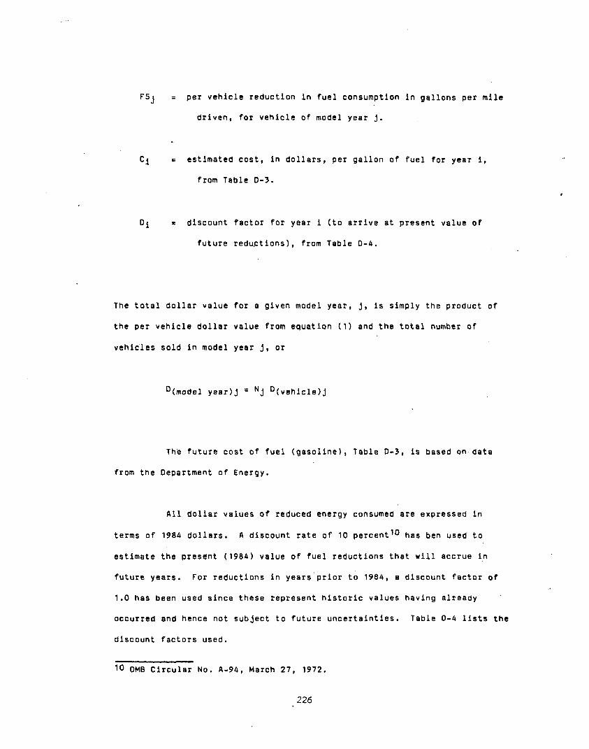
per vehicle reduction in fuel consumption in gallons per mile
driven, for vehicle of model year j.
estimated cost, in dollars, per gallon of fuel for year i,
from Table D-3.
discount factor for year i (to arrive at present value of
future reductions), from Table 0-4.
The total dollar value for a given model year, j, is simply the product of
the per vehicle dollar value from equation (1) and the total number of
vehicles sold in model year j, or
D(model year)j = Nj D(vehicle)j
The future cost of fuel (gasoline), Table D-3, is based on data
from the Department of Energy.
All dollar values of reduced energy consumed are expressed in
terms of 1984 dollars. A discount rate of 10 percent10 has ben used to
estimate the present (1984) value of fuel reductions that will accrue in
future years. For reductions in years prior to 1984, a discount factor of
1.0 has been used since these represent historic values having already
occurred and hence not subject to future uncertainties. Table D-4 lists the
discount factors used.
10 OMB Circular No. A-94, March 27, 1972.
226

TABLE D-3
ESTIMATED AVERAGE PRICE OF UNLEADED GASOLINE, 1984 DOLLARS
Year
19791980198119821983198419851986198719881989199019911992199319941995199619971998199920002001
Price(Dollars/Gallon)
$1,234.558.574.396.33.25 :,191,
1.161.161.191.211.231.291.351.411.471.521.561.601.641.681.731.77
Sources: "Transportation Energy Data Book: Edition 7, Oak RidgeLaboratory, ORNL-6050, Date of Issue - June 1984." (Source ofdata on current year price of unleaded gasoline for years1978-1982.)
"Economic Report of the President, Transmitted to the Congress,February 1985." (Source of price deflator data for adjusting1978-1982 gasoline prices to constant 1984 dollars).
Price data for 1983-1984 adapted from estimates made by NHTSA foruse in regulatory impact analyses of the 1986 CAFE standards.Projections for 1985-1984 were adapted from the U.S. Departmentof Energy (DOE) Middle World Oil Price Case, Gasoline Price Pro-jections for the Transportation Section in "Annual Energy Out-look, 1984," Energy Information Administration, D0E/EIA-9383(84),January 1985. Projections for 1995-2001 are DOE's "referencecase projections," in "Energy Projections to the Year 2010, ATechnical Report in Support of the National Energy Policy Plan,"draft report, April 2, 1985. NHTSA adjusted the projectionsslightly to include only the price of unleaded gasoline; somevalues were interpolated.
227
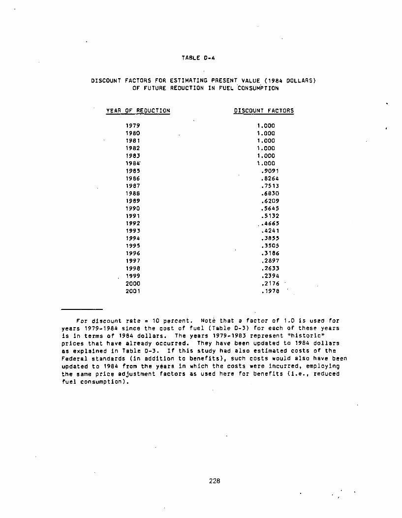
TABLE D-4
DISCOUNT FACTORS FOR ESTIMATING PRESENT VALUE (1984 DOLLARS)OF FUTURE REDUCTION IN FUEL CONSUMPTION
YEAR OF REDUCTION
197919801981198219831984'19851986198719881989199019911992199319941995199619971998
, 199920002001
DISCOUNT FACTORS
111111
.000
.000
.000
.000
.000
.000
.9091
.8264
.7513
.6830
.6209
.5645
.5132
.4665
.4241
.3855
.3505
.3186
.2897
.2633
.2394
.2176 '
.1978 '
For discount rate = 10 percent. Note that a factor of 1.0 is used foryears 1979-1984 since the cost of fuel (Table D-3) for each of these yearsis in terms of 1984 dollars. The years 1979-1983 represent "historic"prices that have already occurred. They have been updated to 1984 dollarsas explained in Table D-3. If this study had also estimated costs of theFederal standards (in addition to benefits), such costs would also have beenupdated to 1984 from the years in which the costs were incurred, employingthe same price adjustment factors as used here for benefits (i.e., reducedfuel consumption).
228