FRP COMPOSITES CHARACTERIZATION BY FTIR-IMAGINGethesis.nitrkl.ac.in/4255/1/...by_ftirimaging.pdf ·...

FRP COMPOSITES CHARACTERIZATION BY

FTIR-IMAGING

A THESIS SUBMITTED IN PARTIAL FULFILMENT OF THE REQUIREMENT FOR THE DEGREE OF

Bachelor of Technology in

Metallurgical and Materials Engineering

By

JITENDRA KUMAR BEHERA

Department of Metallurgical and Materials Engineering

National Institute of Technology

Rourkela

2007

FRP COMPOSITES CHARACTERIZATION BY FTIR-IMAGING

A THESIS SUBMITTED IN PARTIAL FULFILMENT OF THE REQUIREMENT FOR THE DEGREE OF

Bachelor of Technology in

Metallurgical and Materials Engineering

By


Under the Guidance of

Prof. B.C.RAY

Department of Metallurgical and Materials Engineering

National Institute of Technology

Rourkela

2007

National Institute of Technology Rourkela

CERTIFICATE

This is to certify that the thesis entitle, “FRP COMPOSITES CHARACTERIZATION BY FTIR-

IMAGING” submitted by Mr. JITENDRA KUMAR BEHERA in partial fulfillment of the

requirements for the award of Bachelor of Technology Degree in Metallurgical and Materials

Engineering at the National Institute of Technology, Rourkela (Deemed University) is an

authentic work carried out by him under my supervision and guidance.

To the best of my knowledge, the matter embodied in the thesis has not been submitted to any

other University / Institute for the any Degree or Diploma.

Date:

Prof. B.C.RAY Dept. of Metallurgical and Materials Engineering

National Institute of Technology Rourkela-769008

ACKNOWLEDGEMENT

I avail this opportunity to extend my hearty indebtedness to my guide Professor B. C. Ray,

Metallurgical & Materials Engineering Department, for his valuable guidance, constant

encouragement and kind help at different stages for the execution of this dissertation work.

I also express my sincere gratitude to Professor G. S. Agrawal, Head of the Department,

Metallurgical & Materials Engineering, for providing valuable departmental facilities.

I am also grateful to Mr. Samir Pradhan and Mr. Rajesh Pattnaik, Metallurgical & Materials

Engineering Department, for their help in carrying out this work.

I am also grateful to Ms Neeti Sharma and Mr. Surendra Kumar M. for their help in

understanding the various things related to my project.

Last but not least I thank technical assistants of metallurgical Dept. and my friends to help me

directly or indirectly to complete this project successfully.


B.Tech Metallurgical and Materials Engineering

Contents

Abstract………………………………………………………………………………..............i List of Figures…………………………………………………………………………………iii List of Tables…………………………………………………………………………………..iv CHAPTER 1: Introduction………………………………………………….......…..1 CHAPTER 2: LITERATURE SURVEY……………………………..…………....4

2.1 Composites ………………………………………………………………..........5 2.2 Fiber Reinforced Polymer Composites…………….……………………..…….5

2.2.1 Types of Fibers Used in FRP Composites…………………………………........7 2.2.2 Epoxy Resin…………………………………………………………..………..11 2.2.3 Advantages of Composites over Metals……………………………..………....11

2.3 Hygrothermal Diffusion……..……………………………………………...….11 2.3.1 Theory of Moisture Absorption…………………………………………….….12 2.3.2 Effect of Moisture Absorption on FRP’s Properties…………………………..13

2.4 3-Point Bend Test ….………………………………………………………….14 2.5 FTIR Imaging …..…………………………………………………….........….15 2.6 Scanning Electron Microscope………………………………………………...16 2.7 Work done by various persons on interphase study………………………………….18

CHAPTER 3: EXPERIMENTAL PROCEDURE……………………………….20

3.1 Fabrication and Cutting of the Composite……………………….………….…21 3.2 Hygrothermal Treatment …………………………………………………........21 3.3 3-Point Bend Test……………………………………………………………....22 3.4 Characterization by FTIR-Imaging…………………………………………….23 3.5 SEM of the Fractured Surface………………………………………………….24

CHAPTER 4: RESULTS AND DISCUSSION………..………………...25

4.1 Moisture Absorption…………………………………………………………………..26 4.2 Effect of Rate of Loading on ILSS……………………………………………………29 4.3 Effect of Moisture Content on ILSS…………………………………………………..35 4.4 FTIR-Imaging Characterization Results………………………………………………36 4.5 Scanning Electron Microscope Results……………………………………………….42

CHAPTER 5: CONCLUSION………………..………..…………………44 REFERENCES .……………………………………………………….…46

ABSTRACT

It is well known that the high-performance properties of glass-fiber-reinforced polymer

composite materials are not simply the sum of the properties of their constituents. The properties

of composites depend on the ability of the interface to transfer stress from the matrix to the

reinforcement. In fact, it is at the interfacial region where stress concentrations develop because

of differences in the thermal expansion coefficients between the reinforcement and the matrix

phase due to loads applied to the structure, cure shrinkage (in thermosetting matrices), and

crystallization (in some thermoplastic matrices). Coupling agents have two different

functionalities that are designed to chemically bond with the reinforcement at one end and the

organic matrix at the other. The most commonly used coupling agents are bifunctional

organosilicon compounds named silanes. The silane coupling agents of most commercial glass

fibers have three hydrolyzable alkoxy functional groups. These groups allow the silanes to react

with each other and with the glass to form a multilayer network on the glass surface.

In order to study the effect of moisture absorption by the glass-fiber surface to the bulk epoxy,

we used FTIR imaging to investigate this problem. Furthermore, to the best of our knowledge,

there are no studies of the epoxy/glass fiber interface using the “FTIR imaging” technique. This

technique uses a focal-plane array detector (FPA) coupled with a step scan interferometer to

improve FTIR microscopic measurements, yielding spatially resolved spectroscopic information

in the infrared region. In addition, this technique allows one to obtain consecutive IR images of

the microscopic region of interest in intervals of time less than 5 min. For this reason, the FTIR

imaging can be used to study the evolution of several components at the same time in specific

sites in the sample. The composite was fabricated using the conventional HAND LAYOUT

method. The materials used are E-Glass Fiber and Epoxy resin (araldite LY556). The hardener

used is HY951. A sixteen layered structure was formed as per the ASTM standards. The fiber

and the matrix were taken in the ratio of 50:50. The sample was left for drying for 24 Hrs after

the fabrication so that the matrix completely seeps in and become dry. The samples after cutting

and oven drying were divided into 3 parts. One part is kept as such and was wrapped in

Aluminium foil and stored in the Dessicator after weighing all the samples. Second and third part

were first weighed and then given a hygrothermal treatment by placing the samples in the

humidity chamber for 50 Hrs and 100 Hrs respectively at 50°C and 95% humidity. After

i

the Hygrothermal treatment, the dimensions of all the samples were measured

and then they were being tested for 3-Point Bend Test. Then the samples were

characterized using FTIR-Imaging and he fractured surface was studied by SEM.

The ILSS value increases with initial moisture absorption due to the relief of residual stresses but

after a certain stage it decreases due to the loss of adhesion between matrix and fiber. The ILSS

value increases with the strain rate but after a certain stage it decreases because the matrix is

unable to transfer load properly i.e. ILSS value is low at low strain rate as well as high strain rate

as at low strain the load is applied for more time and thus the specimen fails at low stress value

and at high strain rate, the time available for transfer of load is insufficient and the load acts as an

impact and thus specimen fails at low stress. Thus the rate of loading should be optimum. The

FTIR-IMAGING Results Shows that the moisture absorption is more at the interface in low Hrs

treatment as the components of composites have the property to absorb moisture and then

moisture absorption is more in matrix due to more debonding leading to creation of voids at the

interface and thus the water diffuses in easily through the interface to matrix. The SEM Images

of the fractured surfaces shows that the initial moisture absorption results in the increase in the

bond strength as the matrix gets squeezed but after a saturation stage, the moisture absorption

results in the debonding of the matrix-interface bond and also matrix-matrix bond and thus ILSS

value initially increases and then decreases.

ii

List of Figures

Page No.

Fig 2.1 Schematic diagram of FRP Composite 5 Fig 2.2 Effect of Fiber Orientation on the strength of FRP Composites 6 Fig 2.3 Comparison of Loading type on Strength and Modulus of

Elasticity 7

Fig 2.4 Moisture absorption Kinetics 12 Fig 2.5 3-Point Bending Test Setup 14 Fig 2.6 FTIR-Imaging Principle 15 Fig 2.7 FTIR spectrum of bisphenol-A-based epoxy resin cured with

tetraethylenepentamine 17

Fig 2.8 Evolution of the FTIR spectra for the epoxy–amine mixture as a function of the curing process.

19

Fig 2.9 FTIR spectrum of the model poly (aminopropylsiloxane) 19 Fig 3.1 Composite sample after the final treatment 21 Fig 3.2 Humidity Chamber 22 Fig 3.3 FTIR-Imaging working 23 Fig 3.4 Scanning Electron Microscope 24 Fig 4.1 Graph between average moisture absorbed and square root of

time 28

Fig 4.2 . Variation of Average ILSS Value with Crosshead Velocity for Dry sample

30

Fig 4.3 Variation of Average ILSS Value with Crosshead Velocity for 50 Hrs Hygrothermally Treated Sample

32

Fig 4.4 Variation of Average ILSS Value with Crosshead Velocity for 100 Hrs Hygrothermally treated sample

34

Fig 4.5 Variation of ILSS value with the moisture absorption (No. of Hrs of Hygrothermal Treatment)

35

Fig 4.6 FTIR-Image for Dry Sample 36 Fig 4.7 Absorbance vs. Wave number Graph for Dry Sample 36 Fig 4.8 FTIR-Image for 50 Hrs Hygrothermally treated sample 37 Fig 4.9 Absorbance vs. Wave number Graph for 50Hrs

Hygrothermally treated Sample 37

Fig 4.10 FTIR-Image for 100 Hrs Hygrothermally treated sample 38 Fig 4.11 Absorbance vs. Wave number Graph for 100Hrs

Hygrothermally treated Sample 39

Fig 4.12 Absorbance vs. Wave number Graph for interface behavior of the different samples

40

Fig 4.13 Absorbance vs. Wave number Graph for matrix behavior of the different samples

41

Fig 4.14 SEM Images of the fractured surface of Dry sample 42 Fig 4.15 SEM Images of the fractured surface of 50 Hrs

Hygrothermally treated sample 42

Fig 4.16 SEM Images of the fractured surface of 100 Hrs Hygrothermally treated Sample.

43

iii

List of Tables Page No.

Table 2.1 Composition of E-Glass 8

Table 2.2 Comparison of Properties of Glass Fiber 8 Table 2.3 Grades of Carbon Fiber 10 Table 2.4 Comparison of properties of carbon fibers 10

Table 4.1 & 4.2 Moisture Absorption in Case of Dry Samples 26 Table 4.3 & 4.4 Moisture Absorption in case of 50 Hrs Hygrothermal

Treated Samples 26

Table 4.5 & 4.6 Moisture Absorption in case of 100 Hrs Hygrothermal Treated Samples

27

Table 4.7 Average moisture absorbed 27 Table 4.8 ILSS calculation for Dry Sample at different loading

rates. 29

Table 4.9 ILSS calculation for 50 Hrs Hygrothermally treated sample at different loading rates

31

Table 4.10 ILSS calculation for 100 Hrs Hygrothermally treated sample at different loading rates

33

iv

CHAPTER 1

INTRODUCTION

1

1. INTRODUCTIONIt is well known that the high-performance properties of glass-fiber-reinforced polymer

composite materials are not simply the sum of the properties of their constituents. The final

performance of a fiber-reinforced composite depends on the fiber properties and architecture, the

extent of resin cure and resultant matrix properties, the quality of the mold filling, and the nature

of the fiber/polymer matrix interface (the region between the fiber and the matrix). The

properties of composite materials are strongly influenced by the type of adhesion between the

reinforcement and the matrix. In many cases failure occurs in the interface region due to

chemical reactions or plasticizing when impurities (commonly water) penetrate the interface. The

properties of composites depend on the ability of the interface to transfer stress from the matrix

to the reinforcement. In fact, it is at the interfacial region where stress concentrations develop

because of differences in the thermal expansion coefficients between the reinforcement and the

matrix phase due to loads applied to the structure, cure shrinkage (in thermosetting matrices),

and crystallization (in some thermoplastic matrices).

The important effects of the interface on the properties of glass-fiber-reinforced composites have

led to considerable efforts to understand, control, and specifically modify it. Surface treatments

of fiber and particle reinforcements are common methods to improve the general adhesion

properties by increasing electrostatic interactions and/or facilitating chemical bonding between

the constituents. Coupling agents have an effect on the interface structure and properties.

Coupling agents have two different functionalities that are designed to chemically bond with the

reinforcement at one end and the organic matrix at the other. The most commonly used coupling

agents are bifunctional organosilicon compounds named silanes. The silane coupling agents of

most commercial glass fibers have three hydrolyzable alkoxy functional groups. These groups

allow the silanes to react with each other and with the glass to form a multilayer network on the

glass surface. These are used to treat glass fibers to promote adhesion and covalent bonding

between the fibers and the polymeric matrix. It was reported that the silane coupling agents

deposit on the glass surface as three fractional layers, with the molecules connected through

siloxane bonds. Three types of bonding between the coupling agent and matrix resin have been

reported: chemical bondmg, hydrogen bondmg, and interpenetrating polymer network. The

performance of polymeric composites is a function of the interfacial properties. The chemical

bonds formed between the fiberglass and polymeric resin, through the use of a silane coupllng

agent, improves the mechanical strength of composites. Most sigmficantly, the wet strength is

2

improved under moist conditions and the dry strength properties return after dehydration.

Apparently, the hydrolysis of some bonds in the silane/glass interphase is a reversible process.

Hydrolytic attack on glass-reinforced plastic composites has been studied extensively by FTIR

spectroscopy over the past ten years. However, this technique has yielded only a FTIR spectrum

that is a combination of the bulk and interphase of the composites. Since the development of

FTIR micro spectroscopy, detailed analyses of the spatial distribution of chemical species in the

composite have been obtained. This is achieved by utilizing a spatial resolution of ten

micrometers.

In order to study the effect of moisture absorption by the glass-fiber surface to the bulk epoxy,

we used FTIR imaging to investigate this problem. Furthermore, to the best of our knowledge,

there are no studies of the epoxy/glass fiber interface using the “FTIR imaging” technique. This

technique uses a focal-plane array detector (FPA) coupled with a stepscan interferometer to

improve FTIR microscopic measurements, yielding spatially resolved spectroscopic information

in the infrared region. In addition, this technique allows one to obtain consecutive IR images of

the microscopic region of interest in intervals of time less than 5 min. For this reason, the FTIR

imaging can be used to study the evolution of several components at the same time in specific

sites in the sample. The multicomponent detection capability and good temporal resolution were

demonstrated in studies of polymer dissolution, polymer curing, and diffusion processes. In this

work it is proposed to study the effect of moisture absorption on an epoxy system at the interface

formed with a glass fiber and also in the bulk of the matrix.

3

CHAPTER 2

LITERATURE SURVEY

4

2. LITERATURE SURVEY

2.1. Composites

A composite is combination of two materials in which one of the materials, called the reinforcing

phase, is in the form of fibers, sheets, or particles, and is embedded in the other materials called

the matrix phase. The reinforcing material and the matrix material can be metal, ceramic, or

polymer. Composites are used because overall properties of the composites are superior to those

of the individual components. For example: polymer/ceramic composites have a greater modulus

than the polymer component, but aren't as brittle as ceramics. The following are some of the

reasons why composites are selected for certain applications:

High strength to weight ratio (low density high tensile strength)

High creep resistance

High tensile strength at elevated temperatures

High toughness

Three types of composites are:

Particle-reinforced composites

Fiber-reinforced composites

Structural composites

2.2. Fiber-Reinforced Composites:

Reinforcing fibers can be made of metals, ceramics, glasses, or polymers that have been turned

into graphite and known as carbon fibers. Fibers increase the modulus of the matrix material.

The strong covalent bond along the fiber’s length gives them a very high modulus in this

direction because to break or extend the fiber the bonds must also be broken or moved. Fibers are

difficult to process into composites which makes fiber-reinforced composites relatively

expensive. Fiber-reinforced composites are used in some of the most advanced, and therefore

most expensive, sports equipment, such as a time-trial racing bicycle frame which consists of

carbon fibers in a thermoset polymer matrix. Body parts of race cars and some automobiles are

composites made of glass fibers (or fiberglass) in a thermoset matrix.

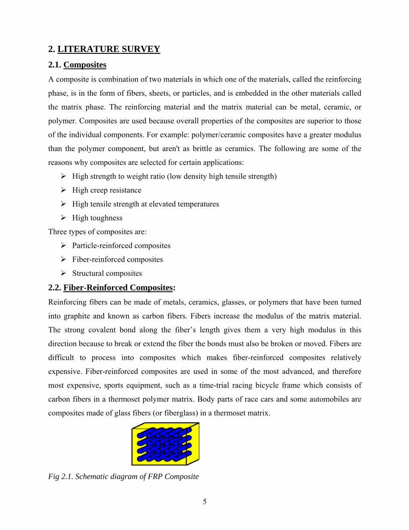
Fig 2.1. Schematic diagram of FRP Composite

5

INFLUENCE OF FIBER LENGTH:

The mechanical characteristics of a fiber reinforced composites depend not only on the

properties of the fiber, but also on the degree to which an applied load is transmitted to the fibers

by the matrix phase. Important to the extent of this load transmittance is the magnitude of the

interfacial bond between the fiber and matrix phases. Some critical fiber length is necessary for

effective strengthening and stiffening of the composite material. This critical length lc is

dependent on the fiber diameter d and its ultimate (or tensile) strength σf*, and on the fiber

matrix bond strength (or shear yield strength of the matrix, whichever is smaller) τc according to

lc = σf*/ 2 τc

for a number of glass and carbon fiber –matrix combinations, this critical length is of the order of

1mm, which ranges between 20 and 150 times the fiber diameter. When a stress equal to σf* is

applied to a fiber having just this critical length maximum fiber load is achieved only at the axial

center of the fiber. Fibers for which l>> lc (normally l> 15lc) are termed continuous;

discontinuous or short fibers have lengths shorter than this. For discontinuous fibers lengths

significantly less than lc, the matrix deforms around the fiber such that there is virtually no stress

transference and little reinforcement by the fiber. To affect a significant improvement in strength

of the composite, the fibers must be continuous.

INFLUENCE OF FIBER ORIENTATION:

Fig 2.2. Effect of Fiber Orientation on the strength of FRP Composites

6

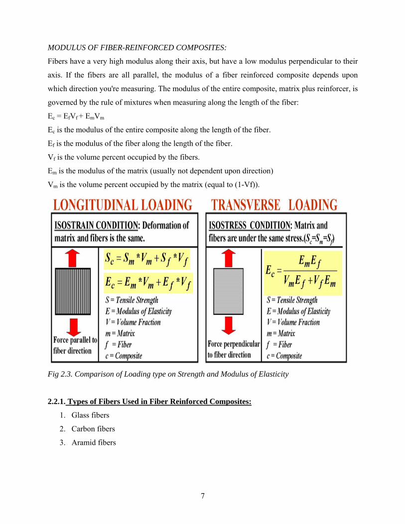
MODULUS OF FIBER-REINFORCED COMPOSITES:

Fibers have a very high modulus along their axis, but have a low modulus perpendicular to their

axis. If the fibers are all parallel, the modulus of a fiber reinforced composite depends upon

which direction you're measuring. The modulus of the entire composite, matrix plus reinforcer, is

governed by the rule of mixtures when measuring along the length of the fiber:

Ec = EfVf + EmVm

Ec is the modulus of the entire composite along the length of the fiber.

Ef is the modulus of the fiber along the length of the fiber.

Vf is the volume percent occupied by the fibers.

Em is the modulus of the matrix (usually not dependent upon direction)

Vm is the volume percent occupied by the matrix (equal to (1-Vf)).

Fig 2.3. Comparison of Loading type on Strength and Modulus of Elasticity

2.2.1. Types of Fibers Used in Fiber Reinforced Composites:

1. Glass fibers

2. Carbon fibers

3. Aramid fibers

7

Glass Fibers

The most common reinforcement for the polymer matrix composites is a glass fiber. Most of the

fibers are based on silica (SiO2), with addition of oxides of Ca, B, Na, Fe, and Al. The glass

fibers are divided into three classes -- E-glass, S-glass and C-glass. The E-glass is designated for

electrical use and the S-glass for high strength. The C-glass is for high corrosion resistance, and

it is uncommon for civil engineering application. Of the three fibers, the E-glass is the most

common reinforcement material used in civil structures. It is produced from lime-alumina-

borosilicate which can be easily obtained from abundance of raw materials like sand. The glass

fiber strength and modulus can degrade with increasing temperature. The fiber itself is regarded

as an isotropic material and has a lower thermal expansion coefficient than that of steel.

1. E-glass (electrical)

Family of glassed with a calcium aluminum borosilicate composition and a maximum

alkali composition of 2%. These are used when strength and high electrical resistivity are required.

2. S-glass (tensile strength)

Fibers have a magnesium aluminosilicate composition, which demonstrates high strength

and used in application where very high tensile strength required.

3. C-glass (chemical)

It has a soda lime borosilicate composition that is used for its chemical stability in corrosive

environment. It is often used on composites that contain or contact acidic materials.

Typical Properties E-Glass S-Glass

Density (g/cm3) 2.60 2.50

Young's Modulus (GPa) 72 87

Tensile Strength (GPa) 1.72 2.53

Tensile Elongation (%) 2.4 2.9

Constituent Weight percentage

SiO2 54

Al203 14

CaO+MgO 12

B2O3 10

Na2O+K2O Less than 2

Impurities Traces

Table 2.1. Composition of E-Glass Table2.2 Comparison of Properties of Glass Fiber

8

Carbon Fibers:

Carbon fiber is the most expensive of the more common reinforcements, but in space

applications the combination of excellent performance characteristics coupled with light weight

make it indispensable reinforcement with cost being of secondary importance Carbon fibers

consist of small crystallite of turbostratic graphite. These resemble graphite single crystals except

that the layer planes are not packed in a regular fashion along the c-axis direction. In a graphite

single crystal the carbon atoms in a basal plane are arranged in hexagonal arrays and held

together by strong covalent bonds. Between the basal planes only weak Vander-waal forces

exist. Therefore the single crystals are highly anisotropic with the plane moduli of the order of

100 GPa whereas the molecules perpendicular to the basal plane are only about 75 GPa. It is thus

evident that to produce high modulus and high strength fibers, the basal planes of the graphite

must be parallel to the fiber axis. They have lower thermal expansion coefficients than both the

glass and aramid fibers. The carbon fiber is an anisotropic material, and its transverse modulus is

an order of magnitude less than its longitudinal modulus. The material has a very high fatigue

and creep resistance. Since its tensile strength decreases with increasing modulus, its strain at

rupture will also be much lower. Because of the material brittleness at higher modulus, it

becomes critical in joint and connection details, which can have high stress concentrations. As a

result of this phenomenon, carbon composite laminates are more effective with adhesive bonding

that eliminates mechanical fasteners.

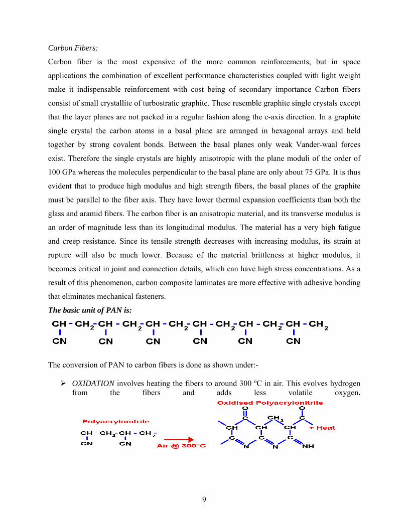
The basic unit of PAN is:

The conversion of PAN to carbon fibers is done as shown under:-

OXIDATION involves heating the fibers to around 300 ºC in air. This evolves hydrogen from the fibers and adds less volatile oxygen.

9

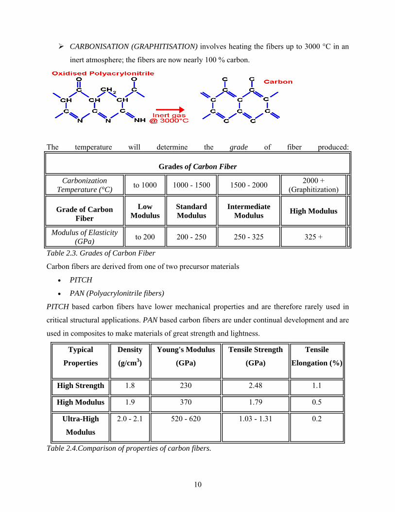
CARBONISATION (GRAPHITISATION) involves heating the fibers up to 3000 °C in an

inert atmosphere; the fibers are now nearly 100 % carbon.

The temperature will determine the grade of fiber produced:

Grades of Carbon Fiber

Carbonization Temperature (°C) to 1000 1000 - 1500 1500 - 2000 2000 +

(Graphitization)

Grade of Carbon Fiber

Low Modulus

Standard Modulus

Intermediate Modulus High Modulus

Modulus of Elasticity (GPa) to 200 200 - 250 250 - 325 325 +

Table 2.3. Grades of Carbon Fiber

Carbon fibers are derived from one of two precursor materials

• PITCH

• PAN (Polyacrylonitrile fibers)

PITCH based carbon fibers have lower mechanical properties and are therefore rarely used in

critical structural applications. PAN based carbon fibers are under continual development and are

used in composites to make materials of great strength and lightness.

Typical

Properties

Density

(g/cm3)

Young's Modulus

(GPa)

Tensile Strength

(GPa)

Tensile

Elongation (%)

High Strength 1.8 230 2.48 1.1

High Modulus 1.9 370 1.79 0.5

Ultra-High

Modulus

2.0 - 2.1 520 - 620 1.03 - 1.31 0.2

Table 2.4.Comparison of properties of carbon fibers.

10

2.2.2. Epoxy Resin

Epoxy or polyepoxide is a thermosetting epoxide polymer that cures (polymerizes and

crosslinks) when mixed with a catalyzing agent or "hardener". Most common epoxy resins are

produced from a reaction between epichlorohydrin and bisphenol-A. The applications for epoxy

based materials are extensive and include coatings, adhesives and composite materials such as

those using carbon fiber and fiberglass reinforcements, (although polyester, vinyl ester, and other

thermosetting resins are also used for glass-reinforced plastic). The chemistry of epoxies and the

range of commercially available variations allows cure polymers to be produced with a very

broad range of properties. In general, epoxies are known for their excellent adhesion, chemical

and heat resistance, good to excellent mechanical properties and very good electrical insulating

properties, but almost any property can be modified (for example silver-filled epoxies with good

electrical conductivity are widely available even though epoxies are typically electrically

insulating).

2.2.3. Advantages of Composites over Metals

1. Fewer components involved because complex shapes can be manufactured in single

molding operations.

2. Freedom of shape because of the manufacture processes available.

3. Inexpensive prototypes because trial fabrication can be done with cheap machine tools.

2.3. Hygrothermal Diffusion

Hygrothermal Diffusion usually takes place in presence of thermal and moisture gradients. In

many cases water absorption obeys Fick’s Law and diffusion is driven by the moisture

concentration gradient between the environment and material producing continuous absorption

until saturation is reached. The atoms migrate from region of higher concentration to that of

lower concentration. The rate of diffusion increases rapidly with the rise in temperature. The

concentration gradient of moisture is developed due to the non-uniform distribution of moisture.

The presence of imperfections and internal stresses also accelerates the process of diffusion.

Epoxy resin absorbs water from the atmosphere from the surface layer reaching equilibrium with

the surrounding environment very quickly followed by diffusion of water into all the material.

The water absorbed is not usually in liquid form but consists of molecules or group of molecules

11

http://en.wikipedia.org/wiki/Thermosetting_plastic

linked by hydrogen bonds to the polymer. In addition water can be absorbed by capillary action

along any crack which may be present or along the fiber-matrix interface.

The Fickian diffusion process is influenced mainly by two factors:

(a) The internal (fiber volume fraction and its orientation)

(b) The external (relative humidity and temperature).

2.3.1. Theory of Moisture Absorption: Percentage weight gain was determined as: (Weight of specimen – Weight of dry specimen) M = x 100 (Weight of dry specimen)

Fig 2.4 Moisture absorption Kinetics

Description of the different stages in moisture absorption kinetics:

Stage 1: Moisture absorption is Fickian.

Stage 2: There is a deviation from linearity with the time axis (reaching saturation, so

decrease in slope).

12

Stage 3: Total non-Fickian pattern (there is a development of micro cracks which enable

rapid moisture diffusion, so rapid increase in percentage of moisture). Non-Fickian behavior:

Fickian behavior is observed in the rubbery state of polymers but often fails to diffusion behavior

in glassy polymers. The deviation from Fickian behavior occurs when:-

(a) Cracks or delamination develops.

(b) Moisture diffusion takes place along the fiber matrix interface.

(c) Presence of voids in the matrix.

The nature of diffusion behavior whether Fickian or non Fickian depends on the relative rate at

which the polymer structure and the moisture distributions change. When the diffusion rates are

much slower than the rate of relaxation, the diffusion has to be Fickian. Non Fickian behavior

pertains to the situations when the relaxation processes progress at a rate comparable to the

diffusion process. Hygrothermal diffusion in polymeric composites is mostly Fickian type, but

non-Fickian behavior is also common for glass/epoxy composite. Absorbed moisture in the

composite certainly deteriorates the matrix dominated properties but he effect is more

pronounced at higher temperatures and at lower strain rates. The ILSS values are the worst

affected property due to this moisture absorption.

2.3.2. Effect of moisture absorption on FRP’s properties:

It is now well known that the exposure of polymeric composites in moist environments, under

both normal and sub-zero conditions, leads to certain degradation of its mechanical properties

which necessitates proper understanding of the correlation between the moist environment and

the structural integrity. It is well known that there is a degradation of material property during its

service life, as it is often subjected to environments with high temperature and humidity or

having a sharp rise and fall of temperature (thermal spikes The absorption of moisture can be

attributed largely to the affinity for moisture of specific functional groups of a highly polar

nature in the cured resin. The absorption of moisture causes plasticization of the resin to occur

with a concurrent swelling and lowering the glass transition temperature of the resin. This

adversely affects the fiber-matrix adhesion properties, resulting debonding at fiber/matrix

interfaces, micro-cracking in the matrix, fiber fragmentations, continuous cracks and several

other phenomena that actually degrades the mechanical property of the composites.

13

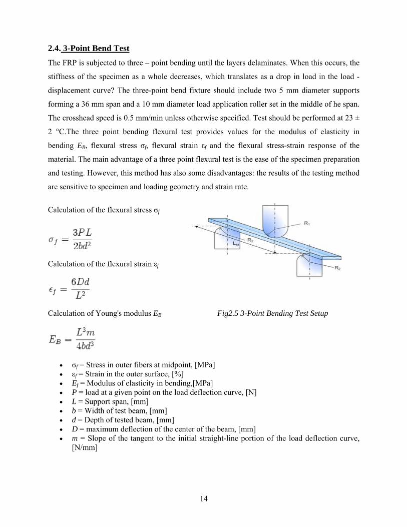
2.4. 3-Point Bend Test

The FRP is subjected to three – point bending until the layers delaminates. When this occurs, the

stiffness of the specimen as a whole decreases, which translates as a drop in load in the load -

displacement curve? The three-point bend fixture should include two 5 mm diameter supports

forming a 36 mm span and a 10 mm diameter load application roller set in the middle of he span.

The crosshead speed is 0.5 mm/min unless otherwise specified. Test should be performed at 23 ±

2 °C.The three point bending flexural test provides values for the modulus of elasticity in

bending EB, flexural stress σB f, flexural strain εf and the flexural stress-strain response of the

material. The main advantage of a three point flexural test is the ease of the specimen preparation

and testing. However, this method has also some disadvantages: the results of the testing method

are sensitive to specimen and loading geometry and strain rate.

Calculation of the flexural stress σf

Calculation of the flexural strain εf

Calculation of Young's modulus EB Fig2.5 3-Point Bending Test Setup

• σf = Stress in outer fibers at midpoint, [MPa] • εf = Strain in the outer surface, [%] • Ef = Modulus of elasticity in bending,[MPa] • P = load at a given point on the load deflection curve, [N] • L = Support span, [mm] • b = Width of test beam, [mm] • d = Depth of tested beam, [mm] • D = maximum deflection of the center of the beam, [mm] • m = Slope of the tangent to the initial straight-line portion of the load deflection curve,

[N/mm]

14

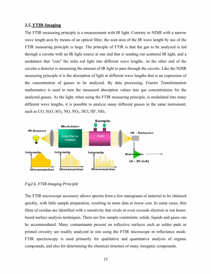
2.5. FTIR-Imaging

The FTIR measuring principle is a measurement with IR light. Contrary to NDIR with a narrow

wave length area by means of an optical filter, the scan area of the IR wave length by use of the

FTIR measuring principle is large. The principle of FTIR is that the gas to be analyzed is led

through a cuvette with an IR light source at one end that is sending out scattered IR light, and a

modulator that "cuts" the infra red light into different wave lengths. At the other end of the

cuvette a detector is measuring the amount of IR light to pass through the cuvette. Like the NDIR

measuring principle it is the absorption of light at different wave lengths that is an expression of

the concentration of gasses to be analyzed. By data processing, Fourier Transformation

mathematics is used to turn the measured absorption values into gas concentrations for the

analyzed gasses. As the light, when using the FTIR measuring principle, is modulated into many

different wave lengths, it is possible to analyze many different gasses in the same instrument;

such as CO, H2O, SO2, NO, NO2, HCl, HF, NH3.

Fig2.6. FTIR-Imaging Principle

The FTIR microscope accessory allows spectra from a few nanograms of material to be obtained

quickly, with little sample preparation, resulting in more data at lower cost. In some cases, thin

films of residue are identified with a sensitivity that rivals or even exceeds electron or ion beam-

based surface analysis techniques. There are few sample constraints; solids, liquids and gases can

be accommodated. Many contaminants present on reflective surfaces such as solder pads or

printed circuitry are readily analyzed in situ using the FTIR microscope in reflectance mode.

FTIR spectroscopy is used primarily for qualitative and quantitative analysis of organic

compounds, and also for determining the chemical structure of many inorganic compounds.

15

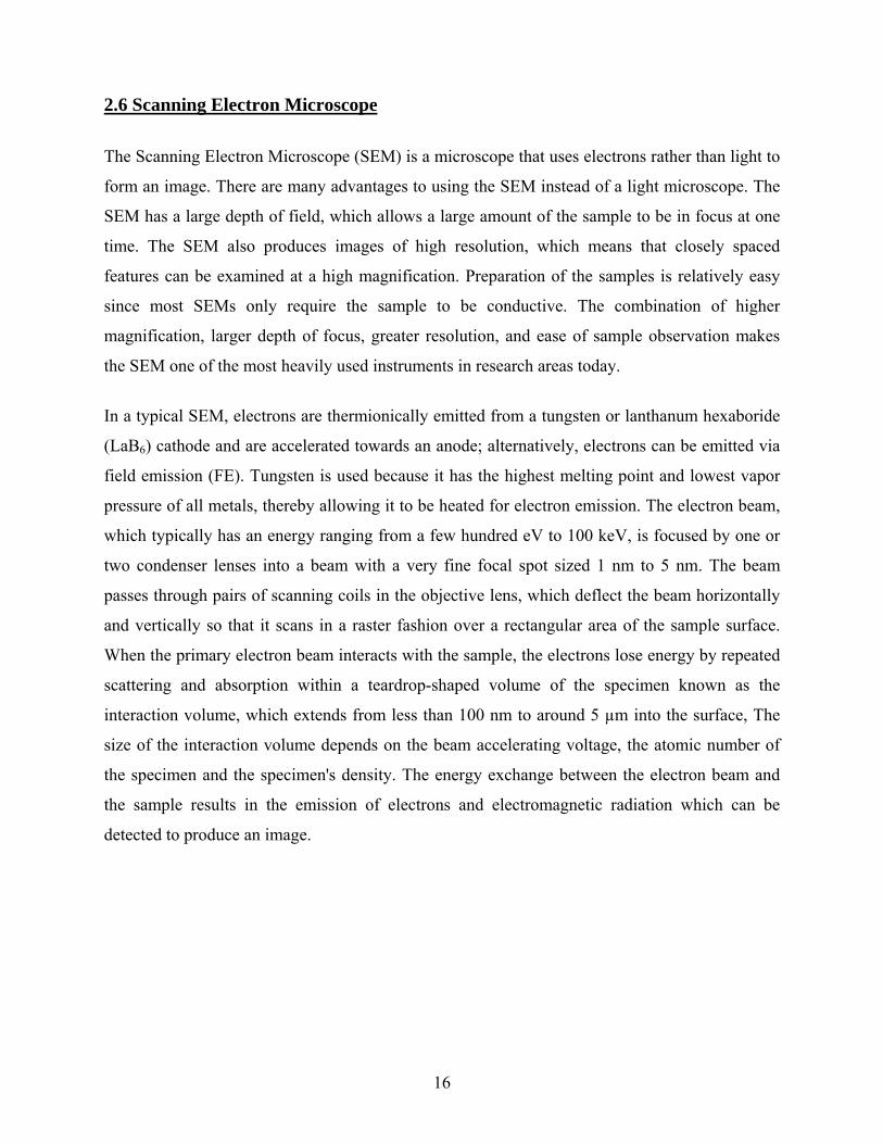
2.6 Scanning Electron Microscope

The Scanning Electron Microscope (SEM) is a microscope that uses electrons rather than light to

form an image. There are many advantages to using the SEM instead of a light microscope. The

SEM has a large depth of field, which allows a large amount of the sample to be in focus at one

time. The SEM also produces images of high resolution, which means that closely spaced

features can be examined at a high magnification. Preparation of the samples is relatively easy

since most SEMs only require the sample to be conductive. The combination of higher

magnification, larger depth of focus, greater resolution, and ease of sample observation makes

the SEM one of the most heavily used instruments in research areas today.

In a typical SEM, electrons are thermionically emitted from a tungsten or lanthanum hexaboride

(LaB6) cathode and are accelerated towards an anode; alternatively, electrons can be emitted via

field emission (FE). Tungsten is used because it has the highest melting point and lowest vapor

pressure of all metals, thereby allowing it to be heated for electron emission. The electron beam,

which typically has an energy ranging from a few hundred eV to 100 keV, is focused by one or

two condenser lenses into a beam with a very fine focal spot sized 1 nm to 5 nm. The beam

passes through pairs of scanning coils in the objective lens, which deflect the beam horizontally

and vertically so that it scans in a raster fashion over a rectangular area of the sample surface.

When the primary electron beam interacts with the sample, the electrons lose energy by repeated

scattering and absorption within a teardrop-shaped volume of the specimen known as the

interaction volume, which extends from less than 100 nm to around 5 µm into the surface, The

size of the interaction volume depends on the beam accelerating voltage, the atomic number of

the specimen and the specimen's density. The energy exchange between the electron beam and

the sample results in the emission of electrons and electromagnetic radiation which can be

detected to produce an image.

16

2.7. Work done by various persons on interphase study:

1. Interfacial Behavior of Epoxy/E-Glass Fiber Composites under Wet-Dry Cycles by FTIR

Micro spectroscopy by W. NOOBUT and J. L. KOENIG, Department of Macromolecular

Science Case, Western Reserve University Cleveland, Ohio 44 106

The interfacial behavior of epoxy/glass fiber micro-composites under cycles of wet and dry

environment change was investigated by Fourier Transform Infrared (FTIR) micro spectroscopy.

The adsorbed water content in the epoxy/fiber interphase under moist conditions is reduced by

treating the glass fibers with a silane coupling agent, -y-aminopropyltriethoxysilane. This results

in a significant decrease in the ring-opening polymerization of epoxy in the epoxy/fiber

interphase. It is also found that the wet-dry cycles cause the significant variation of the residual

adsorbed water in the interphase regions. There is an indication that the debonding in the

epoxy/silane-treated fiber interphase is slower than the epoxy/heat-cleaned fiber interphase.

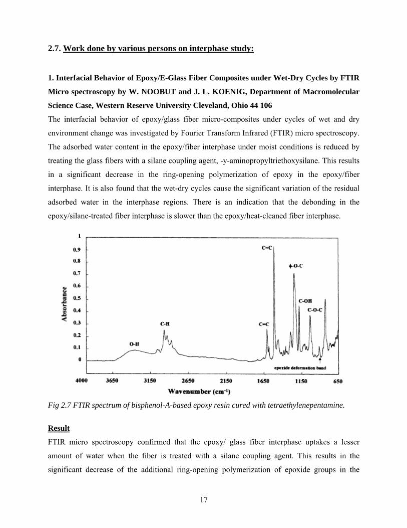
Fig 2.7 FTIR spectrum of bisphenol-A-based epoxy resin cured with tetraethylenepentamine.

Result

FTIR micro spectroscopy confirmed that the epoxy/ glass fiber interphase uptakes a lesser

amount of water when the fiber is treated with a silane coupling agent. This results in the

significant decrease of the additional ring-opening polymerization of epoxide groups in the

17

interphase. There was indication of slow debonding in the epoxy/APS-treated and epoxy/as-

received glass fiber interphases relative to that of the epoxy/heat-cleaned fiber interphase. The

rapid degradation of the interfacial properties of the composites is probably caused by the

significant variation of the residual adsorbed water in the interphase region.

2. The nature of the structural gradient in epoxy curing at a glass fiber/epoxy matrix

interface using FTIR imaging by J. Gonzalez-Benito, Department of Materials Science and

Metallurgic Engineering, Universidad Carlos III de Madrid, Avda. Universidad 30, 28911

Leganes, Madrid, Spain

The curing process of an epoxide system was studied at the interface formed between a silane-

coated glass fiber and an epoxy matrix. The gradient in the structure of the epoxy resin as a result

of the cure process at the fiber/matrix interfacial region was monitored by FTIR imaging. For

comparison, the epoxy curing at the interface formed between the epoxy resin and (a) an

uncoated glass fiber and (b) a polyorganosiloxane (obtained from the silane used for the glass-

fiber coating) were also monitored. Chemically specific images of the OH and the H–N–H

groups near the interface region were obtained. These images suggest that there is a chemical

gradient in the structure of the matrix from the fiber surface to the polymer bulk due to different

conversions. The basis of the different kinetics of the curing reactions is a result of amino group

inactivation at the interface. This deactivation translates into an off-stoichiometry of the reaction

mixture, which is a function of the distance from the surface of the glass fiber.

Result

The curing process of an epoxy system at the interface formed with a silane coated glass fiber

was studied by using FTIR imaging. Chemically specific images for OH and H–N–H within the

system were obtained. The analysis of these images suggests that there is a variation in the

chemical structure of the matrix from the fiber to the polymer bulk due to different conversions

arising from a gradient in the initial composition. Furthermore, it was observed that the rate of

the curing reaction changed depending on the distance to the glass fiber and this change was also

associated to changes in the stoichiometry.

18

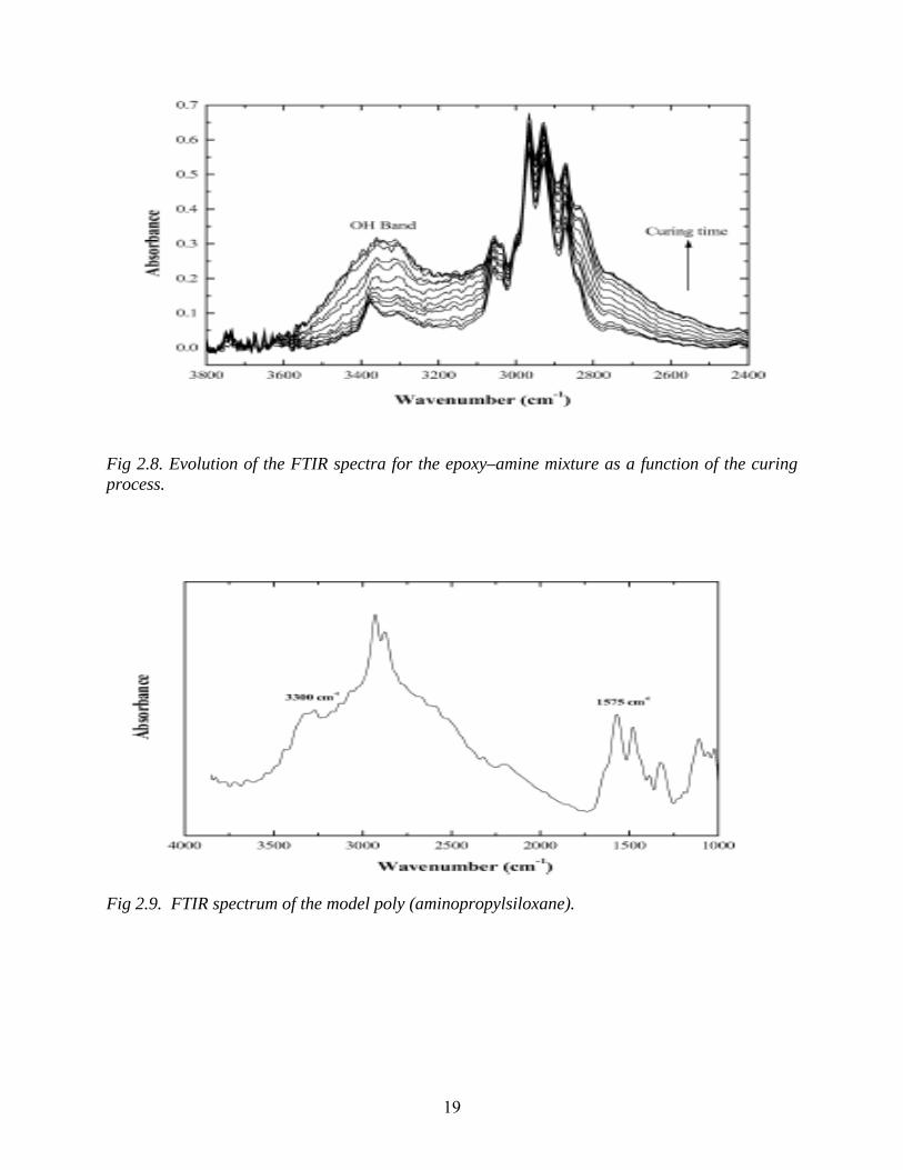
Fig 2.8. Evolution of the FTIR spectra for the epoxy–amine mixture as a function of the curing process.

Fig 2.9. FTIR spectrum of the model poly (aminopropylsiloxane).

19

CHAPTER 3

EXPERIMENTAL PROCEDURE

20

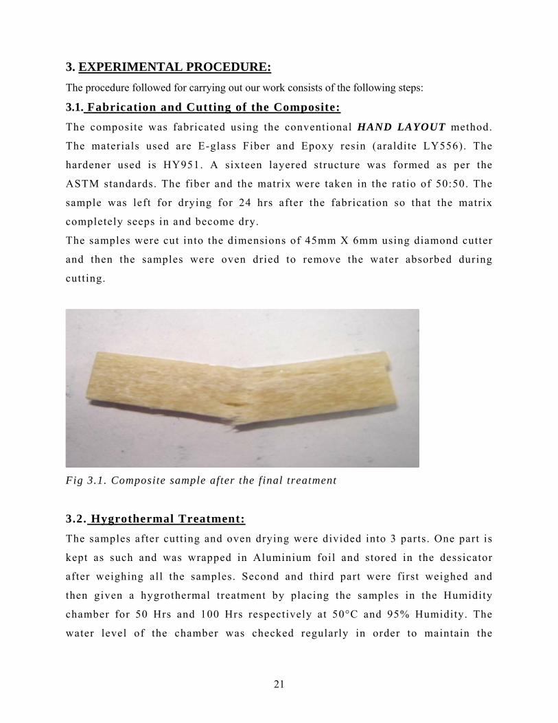
3. EXPERIMENTAL PROCEDURE: The procedure followed for carrying out our work consists of the following steps:

3.1. Fabrication and Cutting of the Composite:

The composite was fabricated using the conventional HAND LAYOUT method.

The materials used are E-glass Fiber and Epoxy resin (araldite LY556). The

hardener used is HY951. A sixteen layered structure was formed as per the

ASTM standards. The fiber and the matrix were taken in the ratio of 50:50. The

sample was left for drying for 24 hrs after the fabrication so that the matrix

completely seeps in and become dry.

The samples were cut into the dimensions of 45mm X 6mm using diamond cutter

and then the samples were oven dried to remove the water absorbed during

cutting.

Fig 3.1. Composite sample after the final treatment

3.2. Hygrothermal Treatment:

The samples after cutting and oven drying were divided into 3 parts. One part is

kept as such and was wrapped in Aluminium foil and stored in the dessicator

after weighing all the samples. Second and third part were first weighed and

then given a hygrothermal treatment by placing the samples in the Humidity

chamber for 50 Hrs and 100 Hrs respectively at 50°C and 95% Humidity. The

water level of the chamber was checked regularly in order to maintain the

21

humidity level. After the treatment is over, the samples were weighed again to

calculate the amount of moisture absorbed.

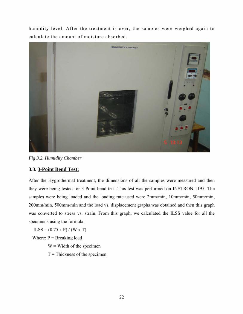
Fig 3.2. Humidity Chamber 3.3. 3-Point Bend Test: After the Hygrothermal treatment, the dimensions of all the samples were measured and then

they were being tested for 3-Point bend test. This test was performed on INSTRON-1195. The

samples were being loaded and the loading rate used were 2mm/min, 10mm/min, 50mm/min,

200mm/min, 500mm/min and the load vs. displacement graphs was obtained and then this graph

was converted to stress vs. strain. From this graph, we calculated the ILSS value for all the

specimens using the formula:

ILSS = (0.75 x P) / (W x T)

Where: P = Breaking load

W = Width of the specimen

T = Thickness of the specimen

22

3.4. Characterization By FTIR-Imaging:

The samples had fractured after 3-Point bend test and then samples were taken for FTIR-Imaging

analysis from these samples. FTIR-Imaging was used to find out the changes that occurred due to

moisture absorption at interface and also in the bulk of the matrix. One sample each of the dry,

50 Hr hygrothermal treatment, 100 Hr hygrothemal treatment were taken and then analyzed

under the FTIR-Imaging machine.

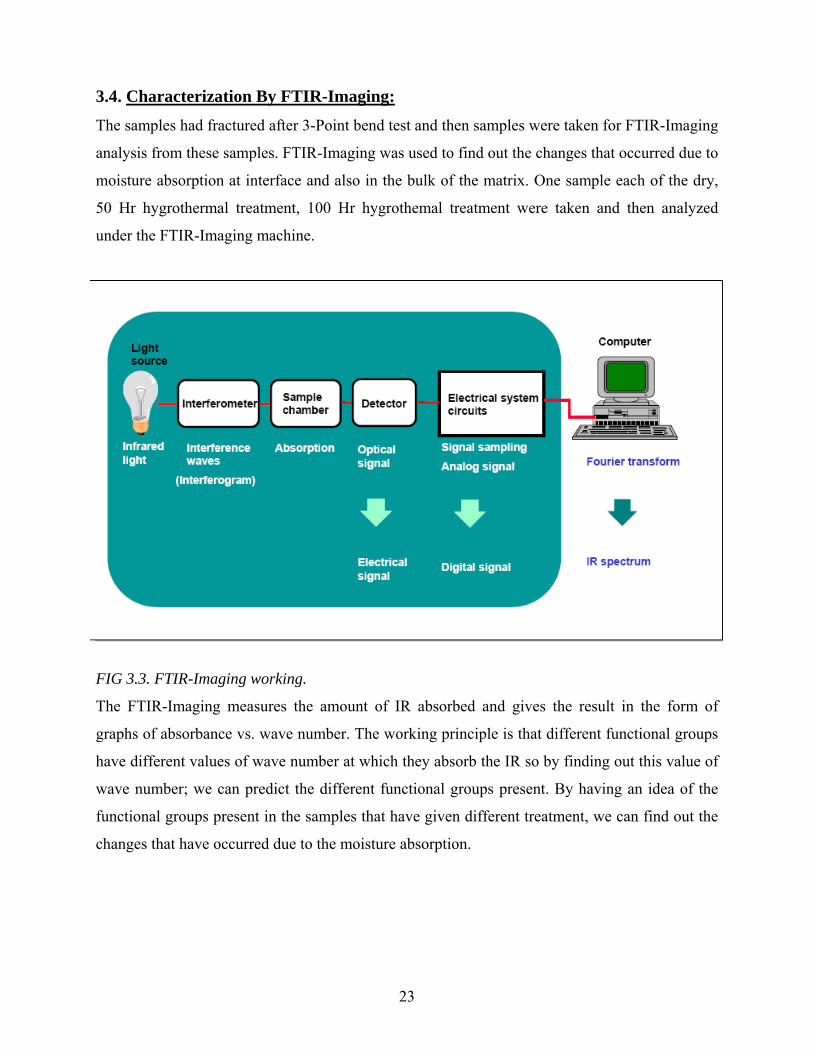
FIG 3.3. FTIR-Imaging working.

The FTIR-Imaging measures the amount of IR absorbed and gives the result in the form of

graphs of absorbance vs. wave number. The working principle is that different functional groups

have different values of wave number at which they absorb the IR so by finding out this value of

wave number; we can predict the different functional groups present. By having an idea of the

functional groups present in the samples that have given different treatment, we can find out the

changes that have occurred due to the moisture absorption.

23

3.5. SEM of the fractured surfaces

To study the fracture surface of the samples being tested above, we carried out the SEM and

these results helped us in the study of the effect of the moisture absorption at different positions.

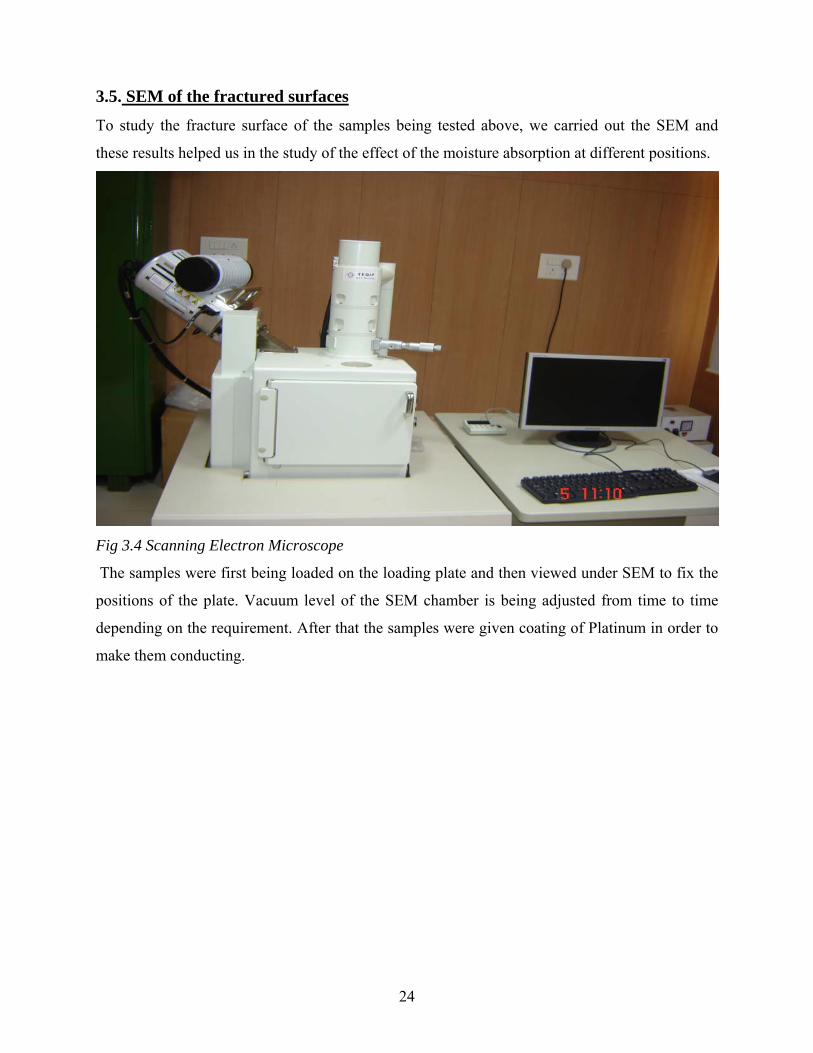
Fig 3.4 Scanning Electron Microscope

The samples were first being loaded on the loading plate and then viewed under SEM to fix the

positions of the plate. Vacuum level of the SEM chamber is being adjusted from time to time

depending on the requirement. After that the samples were given coating of Platinum in order to

make them conducting.

24

CHAPTER 4

RESULTS AND DISCUSSION

25

4. RESULTS AND DISCUSSION 4.1. Moisture Absorption

Sample no:

Initial weight (gms)

Final weight (gm)

% Moisture absorbed

1 3.7632 3.7632 0

2 4.3281 4.3281 0

3 3.6738 3.6738 0

4 4.3017 4.3017 0

5 3.5323 3.5323 0

6 3.5016 3.5016 0

7 3.9112 3.9112 0

8 3.0288 3.0288 0

9 3.3892 3.3892 0

10 3.9215 3.9215 0

Sample no:


Final weight (gm)

% Moisture absorbed

11 4.2998 4.2998 0

12 3.5447 3.5447 0

13 3.5243 3.5243 0

14 4.3713 4.3713 0

15 3.8762 3.8762 0

16 3.3201 3.3201 0

17 3.6752 3.6752 0

18 3.5942 3.5942 0

19 3.5594 3.5594 0

20 3.6591 3.6591 0

Table 4.1 & 4.2. Moisture Absorption in Case of Dry Samples.

Sample no:


Final weight (gm)

% Moisture absorbed

21 2.6657 2.6932 1.031

22 2.9087 2.9408 1.103

23 3.7362 3.7755 1.051

24 3.4543 3.4893 1.103

25 5.1186 5.1642 0.89

26 3.2302 3.2624 0.996

27 3.9903 4.0311 1.02

28 3.3669 3.4031 1.075

29 3.8369 3.8769 1.042

30 3.6393 3.6784 1.074

Sample no:


Final weight (gm)

% Moisture absorbed

31 3.4853 3.5223 1.061

32 3.8057 3.8484 1.122

33 3.6389 3.6776 1.063

34 4.1708 4.2158 1.078

35 3.2235 3.2596 1.119

36 3.8104 3.8492 1.018

37 4.1304 4.1942 1.544

38 4.5596 4.5985 0.853

39 3.3641 3.3964 0.960

40 3.6022 3.6417 1.096

Table 4.3 & 4.4. Moisture Absorption in case of 50 Hrs Hygrothermal Treated Samples

26

Sample no:


Final weight (gm)

% Moisture absorbed

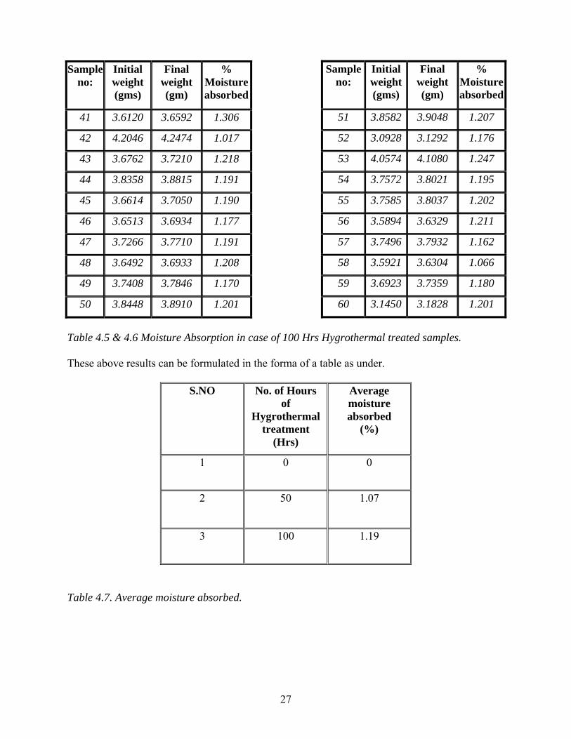
41 3.6120 3.6592 1.306

42 4.2046 4.2474 1.017

43 3.6762 3.7210 1.218

44 3.8358 3.8815 1.191

45 3.6614 3.7050 1.190

46 3.6513 3.6934 1.177

47 3.7266 3.7710 1.191

48 3.6492 3.6933 1.208

49 3.7408 3.7846 1.170

50 3.8448 3.8910 1.201

Sample no:


Final weight (gm)

% Moisture absorbed

51 3.8582 3.9048 1.207

52 3.0928 3.1292 1.176

53 4.0574 4.1080 1.247

54 3.7572 3.8021 1.195

55 3.7585 3.8037 1.202

56 3.5894 3.6329 1.211

57 3.7496 3.7932 1.162

58 3.5921 3.6304 1.066

59 3.6923 3.7359 1.180

60 3.1450 3.1828 1.201

Table 4.5 & 4.6 Moisture Absorption in case of 100 Hrs Hygrothermal treated samples. These above results can be formulated in the forma of a table as under.

S.NO No. of Hours of

Hygrothermal treatment

(Hrs)

Average moisture absorbed

(%)

1 0 0

2 50 1.07

3 100 1.19

Table 4.7. Average moisture absorbed.

27

This table can be represented in the form of a graph and from that graph we can interpret about

the moisture absorption in the treatment given.

% MOISTURE ABSORBED VS SQUARE ROOT OF TIME

0

0.5

1

1.5

0 5 10 15

SQUARE ROOT OF TIME OF HYGROTHERMAL TREATMENT

AV

ER

AGE

%M

OIS

TURE

AB

SORB

ED Fig 4.1 Graph between average moisture absorbed and square root of time Interpretation From the above graph we can interpret the following points.

Initially the rate of moisture absorption is high. This is due to the presence of free spaces

in the composites. The moisture absorption obeys fick’s law i.e. the fickian curve is

obtained.

After a specific time the rate of moisture absorption decreases gradually. This is due to

the saturation of the matrix i.e. the moisture absorbed is sufficient enough to fill the

spaces and very less moisture is required.

So we can conclude that moisture absorption is highest in the beginning and the gradually

goes on decreasing after a specific interval of time due to saturation.

28

4.2. Effect of Rate of Loading on ILSS

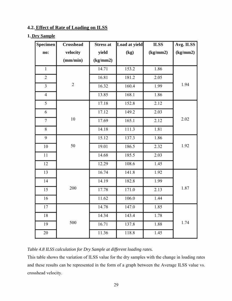
1. Dry Sample

Specimen

no:

Crosshead

velocity

(mm/min)

Stress at

yield

(kg/mm2)

Load at yield

(kg)

ILSS

(kg/mm2)

Avg. ILSS

(kg/mm2)

1 14.71 153.2 1.86

2 16.81 181.2 2.05

3 16.32 160.4 1.99

4

2

13.85 168.1 1.86

1.94

5 17.18 152.8 2.12

6 17.12 149.2 2.03

7 17.69 165.1 2.12

8

10

14.18 111.3 1.81

2.02

9 15.12 137.3 1.86

10 19.01 186.5 2.32

11 14.68 185.5 2.03

12

50

12.29 108.6 1.45

1.92

13 16.74 141.8 1.92

14 14.19 182.8 1.99

15 17.78 171.0 2.13

16

200

11.62 106.0 1.44

1.87

17 14.78 147.0 1.85

18 14.34 143.4 1.78

19 16.71 137.8 1.88

20

500

11.36 118.8 1.45

1.74

Table 4.8 ILSS calculation for Dry Sample at different loading rates.

This table shows the variation of ILSS value for the dry samples with the change in loading rates

and these results can be represented in the form of a graph between the Average ILSS value vs.

crosshead velocity.

29

DRY SAMPLE

1.71.751.8

1.851.9

1.952

2.05

0 100 200 300 400 500 600

CROSSHEAD VELOCITY(mm/min)

ILSS

(mpa

) Fig 4.2. Variation of Average ILSS Value with Crosshead Velocity for Dry sample Interpretation

From the above graph, it is clear that the ILSS value first increases with the increase in

the crosshead velocity and then after 10mm/min, it decreases.

The ILSS value is low at low strain rate as the load applied on the specimen is held for

more time and thus more deterioration will take place and the material will fail at a low

ILSS value

The ILSS value is also low at high rate as very less time is available for the transfer of

load from fiber to matrix and the load applied acts as a impact and thus the material fails

at a low ILSS value.

Thus from above we can conclude that the loading rate should neither be low nor high but

it should be kept optimum so that proper time is available for the transfer of load from

fiber to matrix and also the load is not applied on the material for more time.

Here the optimum loading is found out to be 10mm/min.

30

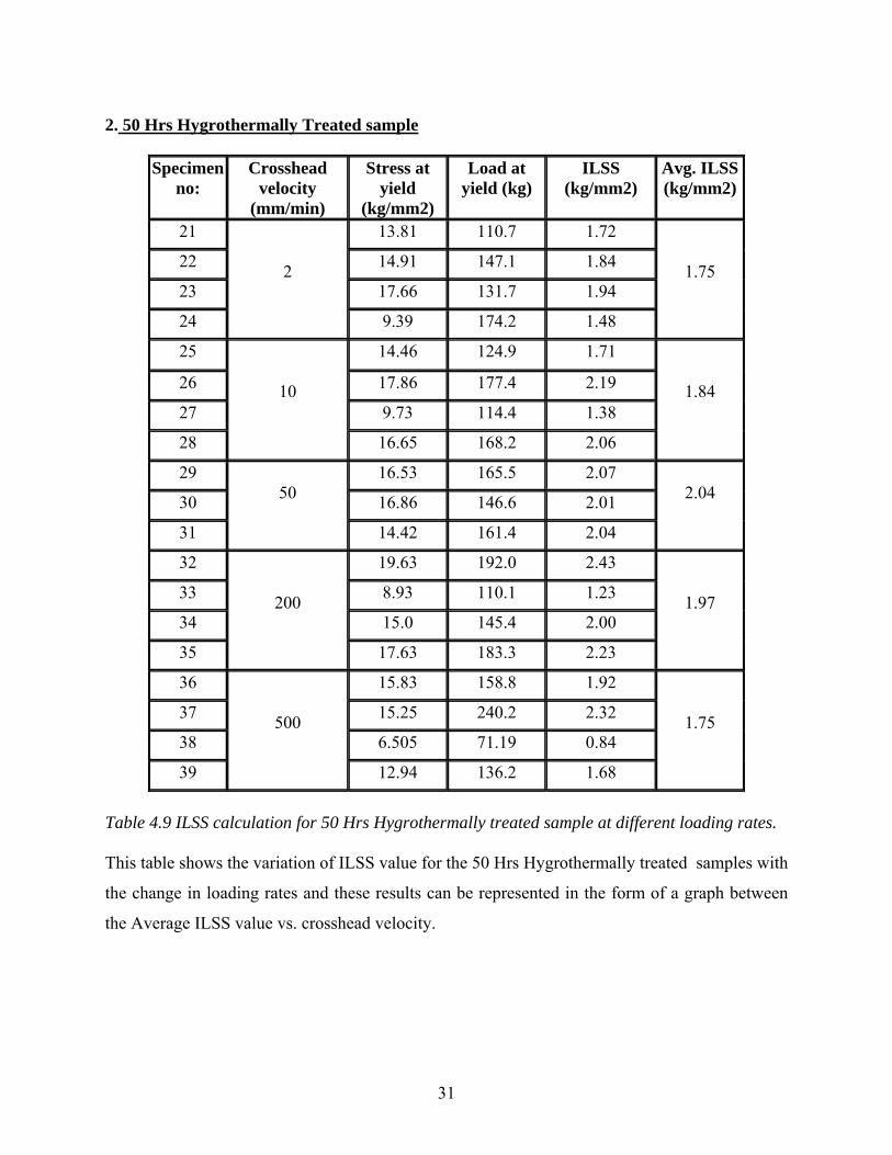
2. 50 Hrs Hygrothermally Treated sample

Specimen no:

Crosshead velocity

(mm/min)

Stress at yield

(kg/mm2)

Load at yield (kg)

ILSS (kg/mm2)

Avg. ILSS (kg/mm2)

21 13.81 110.7 1.72

22 14.91 147.1 1.84

23 17.66 131.7 1.94

24

2

9.39 174.2 1.48

1.75

25 14.46 124.9 1.71

26 17.86 177.4 2.19

27 9.73 114.4 1.38

28

10

16.65 168.2 2.06

1.84

29 16.53 165.5 2.07

30 16.86 146.6 2.01

31

50

14.42 161.4 2.04

2.04

32 19.63 192.0 2.43

33 8.93 110.1 1.23

34 15.0 145.4 2.00

35

200

17.63 183.3 2.23

1.97

36 15.83 158.8 1.92

37 15.25 240.2 2.32

38 6.505 71.19 0.84

39

500

12.94 136.2 1.68

1.75

Table 4.9 ILSS calculation for 50 Hrs Hygrothermally treated sample at different loading rates. This table shows the variation of ILSS value for the 50 Hrs Hygrothermally treated samples with

the change in loading rates and these results can be represented in the form of a graph between

the Average ILSS value vs. crosshead velocity.

31

50 HOURS SAMPLE

1.71.751.8

1.851.9

1.952

2.052.1

0 100 200 300 400 500 600


ILSS

(mpa

) Fig 4.3 Variation of Average ILSS Value with Crosshead Velocity for 50 Hrs Hygrothermally Treated Sample Interpretation





ILSS value








32

3. 100 Hrs Hygrothermally Treated sample

Specimen no:

Crosshead velocity

(mm/min)

Stress at yield

(kg/mm2)

Load at yield (kg)

ILSS (kg/mm2)

Avg. ILSS

(kg/mm2)41 15.14 159.9 1.97 42 12.85 178.9 1.88 43 11.95 137.4 1.65 44

2

15.25 156.3 1.92

1.86

45 18.33 182.0 2.27 46 12.86 142.6 1.68 47 15.46 162.5 1.95 48

10

13.92 153.3 1.90

1.95

49 19.11 194.7 2.40 50 18.76 178.8 2.27 51 19.19 191.6 2.36 52

50

9.34 109.1 1.37

2.10

53 15.25 185.9 2.14 54 16.34 165.9 2.02 55 16.09 155.2 1.97 56

200

16.04 137.2 1.85

2.00

57 14.59 146.5 1.81 58 13.57 108.6 1.46 59 14.13 151.6 1.82 60

500

10.40 105.5 1.37

1.62

Table 4.10 ILSS calculation for 100 Hrs Hygrothermally treated sample at different loading rates. This table shows the variation of ILSS value for the 100 Hrs Hygrothermally treated samples

with the change in loading rates and these results can be represented in the form of a graph

between the Average ILSS value vs. crosshead velocity.

33

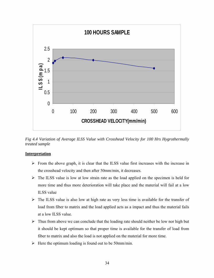
100 HOURS SAMPLE

0

0.5

1

1.5

2

2.5

0 100 200 300 400 500 600


ILSS

(mpa

) Fig 4.4 Variation of Average ILSS Value with Crosshead Velocity for 100 Hrs Hygrothermally treated sample Interpretation





ILSS value








34

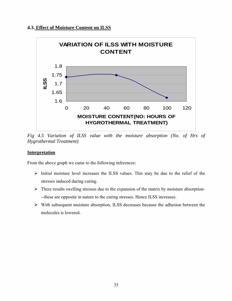
4.3. Effect of Moisture Content on ILSS

VARIATION OF ILSS WITH MOISTURE CONTENT

1.6

1.65

1.7

1.75

1.8

0 20 40 60 80 100 120

MOISTURE CONTENT(NO: HOURS OF HYGROTHERMAL TREATMENT)

ILS

S Fig 4.5 Variation of ILSS value with the moisture absorption (No. of Hrs of Hygrothermal Treatment) Interpretation From the above graph we came to the following inferences:

Initial moisture level increases the ILSS values. This may be due to the relief of the

stresses induced during curing.

There results swelling stresses due to the expansion of the matrix by moisture absorption-

--these are opposite in nature to the curing stresses. Hence ILSS increases.

With subsequent moisture absorption, ILSS decreases because the adhesion between the

molecules is lowered.

35

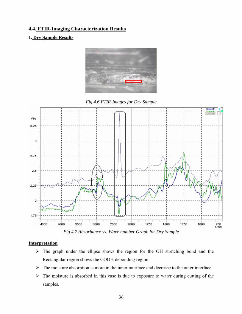
4.4. FTIR-Imaging Characterization Results

1. Dry Sample Results

Fig 4.6 FTIR-Images for Dry Sample

Fig 4.7 Absorbance vs. Wave number Graph for Dry Sample

Interpretation

The graph under the ellipse shows the region for the OH stretching bond and the

Rectangular region shows the COOH debonding region.

The moisture absorption is more in the inner interface and decrease to the outer interface.

The moisture is absorbed in this case is due to exposure to water during cutting of the

samples.

36

The moisture content is more in the inner Interface as the moisture from outer interface

and the matrix is removed when the sample was dried in oven.

The debonding has occurred in the outer interface and the matrix, so the moisture

absorbed is more in the inner interface.

The debonding results in the formation of voids or free surfaces and thus the diffusion of

water becomes easier and it seeps into the inner interface through matrix.

2. 50 Hrs Hygrothermally treated samples results

Fig 4.8 FTIR-Image for 50 Hrs Hygrothermally treated sample

Fig 4.9 Absorbance vs. Wave number Graph for 50Hrs Hygrothermally treated Sample

37

Interpretation



The moisture absorption is more in the outer interface and decrease to the inner interface.

The moisture content is more in the outer interface due to the presence of voids present in

the samples and also the ability of the matrix to absorb moisture is more in the beginning.

The debonding has occurred in the matrix, so the moisture has moved inside the matrix.

Two regions have formed in the matrix and they are differentiated by the amount of the

moisture absorbed.


water becomes easier and it seeps into the inner interface through matrix.

The moisture absorbed is more at the interface and less in the matrix due to the ability of

the interface to absorb moisture as it contains voids and free surfaces.

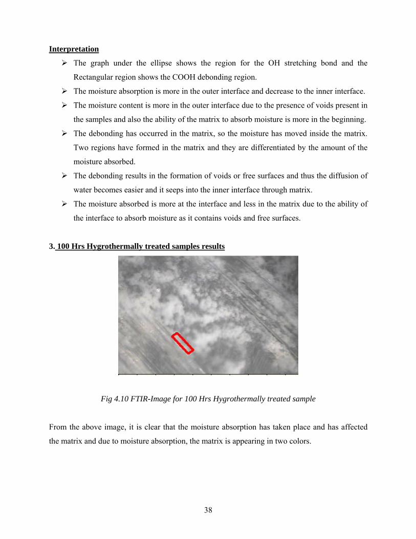
3. 100 Hrs Hygrothermally treated samples results

Fig 4.10 FTIR-Image for 100 Hrs Hygrothermally treated sample

From the above image, it is clear that the moisture absorption has taken place and has affected

the matrix and due to moisture absorption, the matrix is appearing in two colors.

38

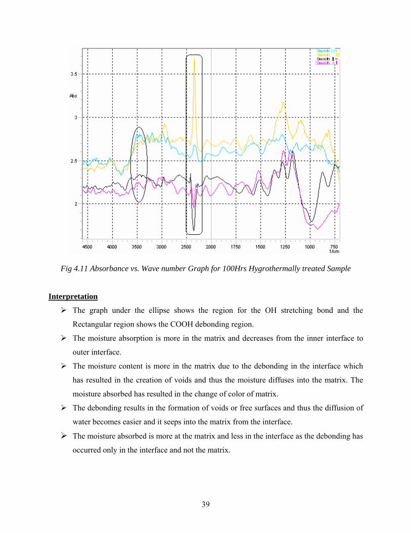
Fig 4.11 Absorbance vs. Wave number Graph for 100Hrs Hygrothermally treated Sample Interpretation



The moisture absorption is more in the matrix and decreases from the inner interface to

outer interface.

The moisture content is more in the matrix due to the debonding in the interface which

has resulted in the creation of voids and thus the moisture diffuses into the matrix. The

moisture absorbed has resulted in the change of color of matrix.


water becomes easier and it seeps into the matrix from the interface.

The moisture absorbed is more at the matrix and less in the interface as the debonding has

occurred only in the interface and not the matrix.

39

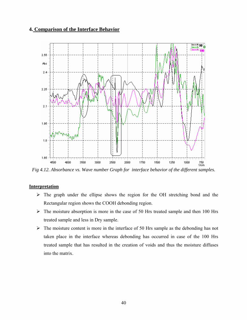
4. Comparison of the Interface Behavior

Fig 4.12. Absorbance vs. Wave number Graph for interface behavior of the different samples.

Interpretation



The moisture absorption is more in the case of 50 Hrs treated sample and then 100 Hrs

treated sample and less in Dry sample.

The moisture content is more in the interface of 50 Hrs sample as the debonding has not

taken place in the interface whereas debonding has occurred in case of the 100 Hrs

treated sample that has resulted in the creation of voids and thus the moisture diffuses

into the matrix.

40

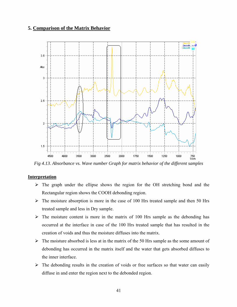
5. Comparison of the Matrix Behavior

Fig 4.13. Absorbance vs. Wave number Graph for matrix behavior of the different samples

Interpretation



The moisture absorption is more in the case of 100 Hrs treated sample and then 50 Hrs

treated sample and less in Dry sample.

The moisture content is more in the matrix of 100 Hrs sample as the debonding has

occurred at the interface in case of the 100 Hrs treated sample that has resulted in the

creation of voids and thus the moisture diffuses into the matrix.

The moisture absorbed is less at in the matrix of the 50 Hrs sample as the some amount of

debonding has occurred in the matrix itself and the water that gets absorbed diffuses to

the inner interface.

The debonding results in the creation of voids or free surfaces so that water can easily

diffuse in and enter the region next to the debonded region.

41

4.5. Scanning Electron Microscope Results

1. Dry Sample

Fig 4.14. SEM Images of the fractured surface of Dry sample.

Interpretation

From the above Images, it is clear that the matrix is strongly bonded to the fibers at

the interface and this result in the increase of strength and fracture is ductile.

Some amount of moisture absorbed during cutting has resulted in the removal of

matrix from the interface and thus decreasing strength at those points.

2. 50 Hrs Hygrothermally treated Sample

Fig 4.15. SEM Images of the fractured surface of 50 Hrs Hygrothermally treated sample.

42

Interpretation

From the above Images, it is clear that the matrix has squeezed due to the moisture

absorption and increases the bonding between fibers and matrix and this result in the

increase of ILSS value and ductile fracture results.

Due to moisture absorption some of the fibers have loosen contact with the matrix

and thus this results in the decrease of strength.

The overall result of the two is increase of the ILSS value.

3. 100 Hrs Hygrothermally treated Sample

Fig 4.16. SEM Images of the fractured surface of 100 Hrs Hygrothermally treated Sample.

Interpretation

From the above Images, it is clear that the matrix has loosen contact with the fiber

due to moisture absorption and this has occurred due to the debonding at the interface

and this results in the decrease of ILSS value.

The fibers have completed lost contact with the other fibers and the matrix. The

matrix-matrix bonding is also diminished.

The above two factors results in the decrease of the ILSS value.

43

CHAPTER 5

CONCLUSION

44

5. CONCLUSION

The ILSS value increases with initial moisture absorption due to the relief of residual

stresses but after a certain stage it decreases due to the loss of adhesion between matrix

and fiber.

The ILSS value increases with the strain rate but after a certain stage it decreases because

the matrix is unable to transfer load properly i.e. ILSS value is low at low strain rate as

well as high strain rate as at low strain the load is applied for more time and thus the

specimen fails at low stress value and at high strain rate, the time available for transfer of

load is insufficient and the load acts as an impact and thus specimen fails at low stress.

Thus the rate of loading should be optimum.

From the FTIR-IMAGING Results, it is clear that the moisture absorption is more at the

interface in low Hrs treatment as the components of composites have the property to

absorb moisture and then moisture absorption is more in matrix due to more debonding

leading to creation of voids at the interface and thus the water diffuses in easily through

the interface to matrix.

From the SEM Images of the fractured surfaces, it is clear that the initial moisture

absorption results in the increase in the bond strength as the matrix gets squeezed but

after a saturation stage, the moisture absorption results in the debonding of the matrix-

interface bond and also matrix-matrix bond and thus ILSS value initially increases and

then decreases.

45

REFERENCES 1. J. Gonzalez-Benito - The nature of the structural gradient in epoxy curing at a glass

fiber/epoxy matrix interface using FTIR imaging, Journal of Colloid and Interface

Science 267 (2003) 326–332.

2. Z.A. Mohd. Ishak, B.N. Yow, H. P. S. A. Khalil, H.D. Rozman - Hygrothermal Aging

and Tensile Behavior of Injection-Molded Rice Husk-Filled Polypropylene Composites,

Journal of Applied Polymer Science, 81(14), 2000, 742-753.

3. B.N. Yow, U.S. Ishiaku, Z.A. Mohd Ishak, J. Karger-Kocsis - Kinetics of Water

Absorption and Hygrothermal Aging Rubber Toughened Poly(Butylene Terephthalate)

With and Without Short Glass Fiber Reinforcement, Composites Science and

Technology, 60(6), 2003, 803-815.

4. B.F. Boukhoulda, E. Adda-Bedia, K. Madani - The Effect of Fiber Orientation Angle in

Composite Materials on Moisture Absorption and Material Degradation After

Hygrothermal Ageing, Journal of Reinforced Plastics and Composites, 74(4), 2006, 406-

418.

5. B.C. Ray - Hydrothermal Fatigue on Interface of Glass-Epoxy Laminates, Journal of

Reinforced Plastics and Composites, 24(10), 2005, 1051-1056

6. Liang Li, ShuYong Zhang, YueHui Chen, MoJun Liu, YiFu Ding, XiaoWen Luo, Zong

Pu, WeiFang Zhou, and Shanjun Li - Water Transportation in Epoxy Resin, Chemistry of

Materials, 17(4), 2005, 839-845.

7. B.C. Ray – Effect of Crosshead Velocity & Subzero Temperature on Mechanical

Behavior of Hygrothermally Conditioned FRPs, Material Science and Engineering A,

379(1-2), 2004, 39-44.

8. S. Pavlidou, C.D. Papaspyrides - The Effect of Hygrothermal History on Water Sorption

and Interlaminar Shear Strength of Glass/Polyester Composites with Different Interfacial

Strength, Composites A, 34(11), 2003, 1117–1124

9. Katya I. Ivanova, Richard A. Pethrick, Stanley Affrossman - Hygrothermal Aging of

Rubber Modified and Mineral Filled Dicyandiamide Cured Digylcidyl Ether of Bisphenol

A Epoxy Resin. I. Diffusion Behavior, Journal of Applied Polymer Science, 82(14),

2001, 3468-3476.

10. B.C. Ray - Loading Rate Effects on Mechanical Properties of Polymer Composites at

Ultra Low Temperatures, Journal of Applied Polymer Science, 100(3), 2006, 2289-2292.

46

11. B.C. Ray – Adhesion of Glass/Epoxy Composites Influenced by Thermal and Cryogenic

Environment, Journal of Applied Polymer Science, 102(2), 2006, 1943-1949.

12. W.Noobut, J.L.Koeing - Interfacial Behavior of Epoxy/E-Glass Fiber Composites under

Wet-Dry Cycles by FTIR Micro spectroscopy.

13. Peiyi Wu, H.W. Siesler- Water diffusion into epoxy resin: a 2D correlation ATR-FTIR

investigation.

14. Hui-Shen Shen, M.Asce - Hygrothermal Effects on the Nonlinear Bending of Shear

Deformable Laminated Plates

15. Sergei G. Kazariana, K.L. Andrew Chana, Veronique Maquetb, Aldo R. Boccaccinic -

Characterization of bioactive and resorbable polylactide/Bioglasss composites by FTIR

spectroscopic imaging.

16. Mikhail V. Motyakin 1, Shulamith Schlick - ESR imaging and FTIR study of thermally

treated poly(acrylonitrile-butadiene-styrene) (ABS) containing a hindered amine

stabilizer: Effect of polymer morphology, and butadiene and stabilizer content.

17. Gang Xu, Wenfang Shi, Ming Gong, Fei Yu and Jianping Feng - Curing behavior and

toughening performance of epoxy resins containing hyper branched polyester Polymer

Advanced Technology 2004; 15: 639–644.

18. Y.C. Lin, Xu Chen - Moisture sorption–desorption–resorption characteristics and its

effect on the mechanical behavior of the epoxy system, Polymer 46 (2005) 11994–12003.

19. B.C. Ray - Temperature Effect During Humid Ageing on Interfaces of Glass and Carbon

Fibers Reinforced Epoxy Composites, Journal of Colloid and Interface Science, 298(1),

2006, 111–117.

20. B.C. Ray - Freeze-thaw Response of Glass-polyester Composites at Different Loading

Rates, Journal of Reinforced Plastics and Composites, 24(16), 2005, 1771-1776

21. B.C. Ray, S. Mula, T. Bera, P.K. Ray – Prior Thermal Spikes and Thermal Shocks on

Mechanical Behavior of Glass Fiber Epoxy Composites, Journal of Reinforced Plastics

and Composites, 25(2), 2006, 197-213

47

FRP COMPOSITES CHARACTERIZATION BY FTIR-IMAGINGethesis.nitrkl.ac.in/4255/1/...by_ftirimaging.pdf ·...

Documents

Transcript of FRP COMPOSITES CHARACTERIZATION BY FTIR-IMAGINGethesis.nitrkl.ac.in/4255/1/...by_ftirimaging.pdf ·...