Frozen Soil Material Testing and Constitutive...

SANDIA REPORTSAND2002-0524Unlimited ReleasePrinted March 2002

Frozen Soil Material Testing andConstitutive Modeling

Moo Y. Lee, Arlo Fossum, Laurence S. Costin and David Bronowski

Prepared bySandia National LaboratoriesAlbuquerque, New Mexico 87185 and Livermore, California 94550

Sandia is a multiprogram laboratory operated by Sandia Corporation,a Lockheed Martin Company, for the United States Department ofEnergy under Contract DE-AC04-94AL85000.

Approved for public release; further dissemination unlimited.

Issued by Sandia National Laboratories, operated for the United States Departmentof Energy by Sandia Corporation.

NOTICE: This report was prepared as an account of work sponsored by an agencyof the United States Government. Neither the United States Government, nor anyagency thereof, nor any of their employees, nor any of their contractors,subcontractors, or their employees, make any warranty, express or implied, orassume any legal liability or responsibility for the accuracy, completeness, orusefulness of any information, apparatus, product, or process disclosed, or representthat its use would not infringe privately owned rights. Reference herein to anyspecific commercial product, process, or service by trade name, trademark,manufacturer, or otherwise, does not necessarily constitute or imply its endorsement,recommendation, or favoring by the United States Government, any agency thereof,or any of their contractors or subcontractors. The views and opinions expressedherein do not necessarily state or reflect those of the United States Government, anyagency thereof, or any of their contractors.

Printed in the United States of America. This report has been reproduced directlyfrom the best available copy.

Available to DOE and DOE contractors fromU.S. Department of EnergyOffice of Scientific and Technical InformationP.O. Box 62Oak Ridge, TN 37831

Telephone: (865)576-8401Facsimile: (865)576-5728E-Mail: [email protected] ordering: http://www.doe.gov/bridge

Available to the public fromU.S. Department of CommerceNational Technical Information Service5285 Port Royal RdSpringfield, VA 22161

Telephone: (800)553-6847Facsimile: (703)605-6900E-Mail: [email protected] order: http://www.ntis.gov/ordering.htm

mailto:[email protected]

mailto:[email protected]

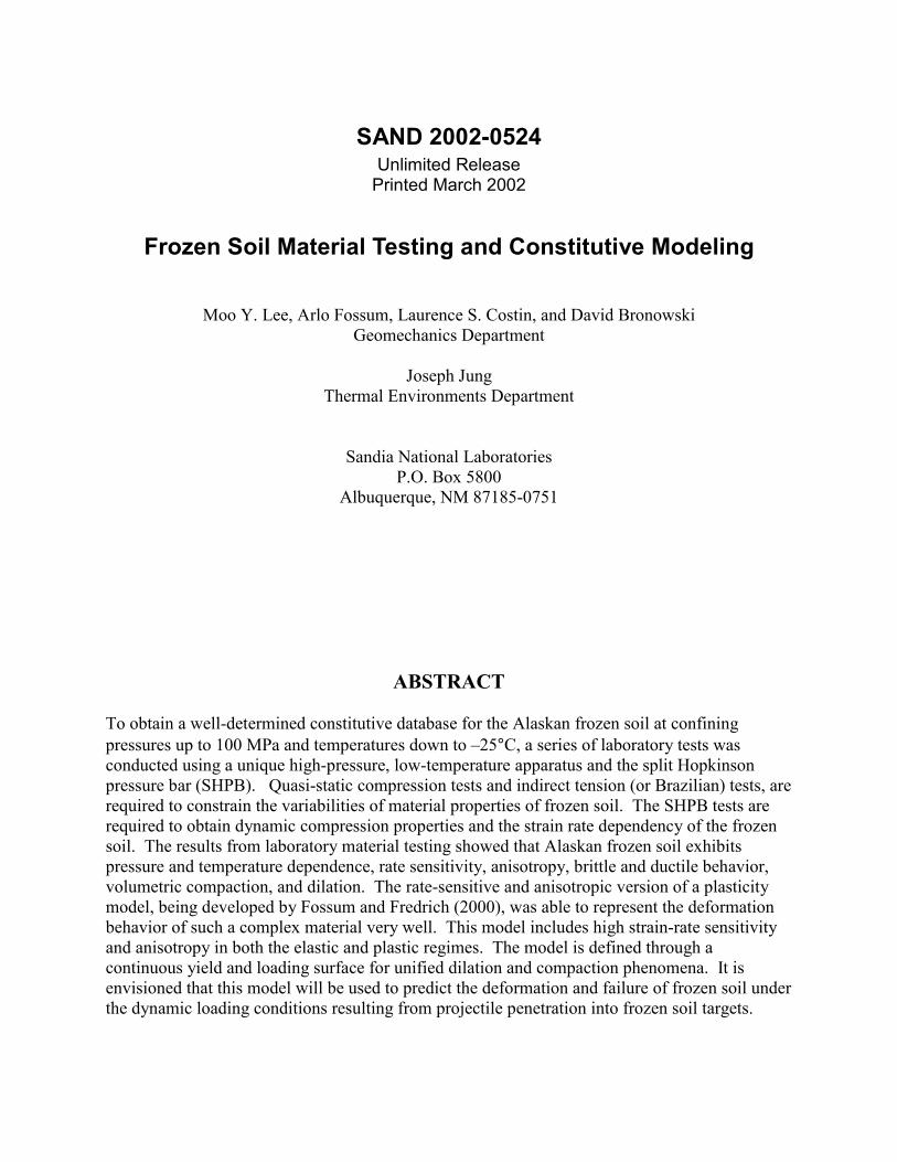
SAND 2002-0524Unlimited Release

Printed March 2002

Frozen Soil Material Testing and Constitutive Modeling

Moo Y. Lee, Arlo Fossum, Laurence S. Costin, and David BronowskiGeomechanics Department

Joseph JungThermal Environments Department

Sandia National LaboratoriesP.O. Box 5800

Albuquerque, NM 87185-0751

ABSTRACT

To obtain a well-determined constitutive database for the Alaskan frozen soil at confiningpressures up to 100 MPa and temperatures down to –25°C, a series of laboratory tests wasconducted using a unique high-pressure, low-temperature apparatus and the split Hopkinsonpressure bar (SHPB). Quasi-static compression tests and indirect tension (or Brazilian) tests, arerequired to constrain the variabilities of material properties of frozen soil. The SHPB tests arerequired to obtain dynamic compression properties and the strain rate dependency of the frozensoil. The results from laboratory material testing showed that Alaskan frozen soil exhibitspressure and temperature dependence, rate sensitivity, anisotropy, brittle and ductile behavior,volumetric compaction, and dilation. The rate-sensitive and anisotropic version of a plasticitymodel, being developed by Fossum and Fredrich (2000), was able to represent the deformationbehavior of such a complex material very well. This model includes high strain-rate sensitivityand anisotropy in both the elastic and plastic regimes. The model is defined through acontinuous yield and loading surface for unified dilation and compaction phenomena. It isenvisioned that this model will be used to predict the deformation and failure of frozen soil underthe dynamic loading conditions resulting from projectile penetration into frozen soil targets.

2

ACKNOWLEDGEMENTS

The authors would like to acknowledge Ned Hansen of Sandia National Laboratories forarranging the sampling activities in the Yukon Test Range at Eielson Air Force Base in Alaska.The authors also appreciate the laboratory assistance of Robert Hardy and Mark Grazier ofSandia National Laboratories. The managerial support received from Jaime L. Moya and JustineE. Johannes are also gratefully appreciated.

3

Table of Contents

1. Introduction ………………………………………………………….......…......…........ 8

2. Sample Preparation and Characterization …………………………...….....…….…..….10

2.1 Sample preparation .....…………………......................…........................….....102.2 Sample characterization...…...................……................................................... 12

3. Development of High Pressure Low Temperature (HPLT) Triaxial Test Cell ..……..... 15

4. Material Testing ………………………………………………..…...........…….……..... 16

4.1 Hydrostatic compression tests ...…………………..…........………………..... 164.2 Brazilian tests……..……………..….............……………………….....…….. 224.3 Unconfined uniaxial compression tests………......…....................................... 264.4 Triaxial compression tests ……….....…………...…...............................…..... 304.5 Quasi-dynamic unconfined uniaxial compression tests..........………........…...334.6 Split Hopkinson pressure bar (SHPB) tests .........…………………………..... 38

5. Constitutive Modeling…………………………………………………..……………… 51

6. Conclusions ……………………………………………………………….….….......... 58

References ………………….……………………..………………………….……............59

APPENDIX…. ……………………………………………………………………………..61

4

Figures

Figure 1. Summary of loading paths used for laboratory testing of frozen soil forconstitutive modeling. I1 is the first invariant of the Cauchy stress tensor andJ2 is the second invariant of the deviatoric stress tensor. Two invariants aredefined as I1 = σ1+σ2+σ3 and J2={(σ1 - σ2)2 + (σ2 - σ3)2 + ( σ3 - σ1)2} / 6 whereσ1, σ2 and σ3 are the maximum, intermediate and minimum principal stresses,respectively……………..……………………………………………………… 9

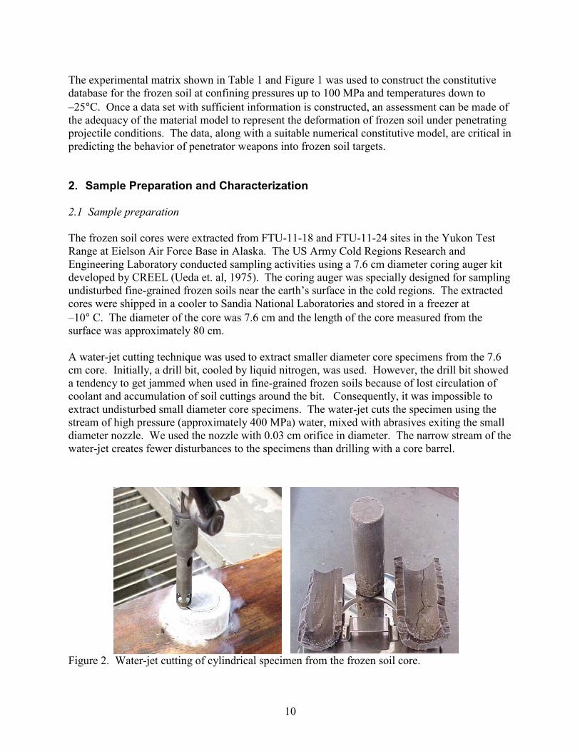
Figure 2. Water-jet cutting of cylindrical specimen from the frozen soil core……………10

Figure 3. Spring-loaded V-block apparatus used to mount the end-caps to the frozen soilspecimen………………………………………………………………………. 11

Figure 4. Alaskan frozen soil specimens extracted from different depths. The specimenon the left represents typical frozen soil found near the surface (within 30 cmin depth) with abundant organic materials. The specimen on the right showsrelatively uniform clay/silt rich frozen soil found below 30 cm in depth………13

Figure 5. Water content of Alaskan frozen soil specimens extracted from differentdepths.………………………………………………………………...……..… 14

Figure 6. Densities of Alaskan frozen soil with respect to depth. The top 30 cm of thesoil is dark-colored with abundant organic material……………………………14

Figure 7. Schematic of the High-Pressure Low-Temperature test cell and aninstrumented frozen soil specimen……………………………….……………..15

Figure 8. External cooling system implemented for the High-Pressure Low-Temperature(HPLT) cell…………………………………………………………………..… 16

Figure 9. Frozen soil specimen mounted between the end-caps for hydrostaticcompression test……………………………………………………………….. 17

Figure 10. Strain vs. hydrostatic pressure recorded during a hydrostatic compressiontesting of a frozen soil specimen………………………………………..………18

Figure 11. Detailed volumetric strain vs. hydrostatic pressure plot showing unloadingand reloading loops for the frozen soil specimen AFS-HS-12. The slope ofthe loop determines the bulk modulus, K……………………………………… 18

Figure 12. Phase diagram for ice under different pressures and temperatures based onDurham et. al. (1983)………………………………………………………...…19

Figure 13. Strain vs. hydrostatic pressure recorded during a hydrostatic compressiontesting of an anisotropic frozen soil specimen………………………………….19

5

Figure 14. Variations of the bulk modulus of Alaskan frozen soil with respect to (a) depth(b) density and (c) temperature.…………………………………………...……21

Figure 15. Brazilian indirect tensile strength test set-up. Shown are the 0.1 MN servo-controlled loading machine, data acquisition system and a failed specimen …..22

Figure 16. Two different types of fracturing behavior of the Alaskan frozen soilsubjected to diametral loading. AFS-BR-17 specimen (a) shows brittle tensilefractures under the low temperature condition (-26°C). AFS-BR-11 specimen(b) shows the network of ductile fractures, with a large amount of plasticdeformation under the high temperature condition (-9°C)…………………….. 23

Figure 17. Typical displacement vs. load record from a Brazilian test conducted for theAlaskan frozen soil at approximately –26°C………………………………..…. 24

Figure 18. Typical displacement vs. load record from a Brazilian test conducted for theAlaskan frozen soil at approximately –10°C. Load was increasedmonotonically without a peak, indicating a ductile deformation without abrittle tensile failure……………………………………………………………. 24

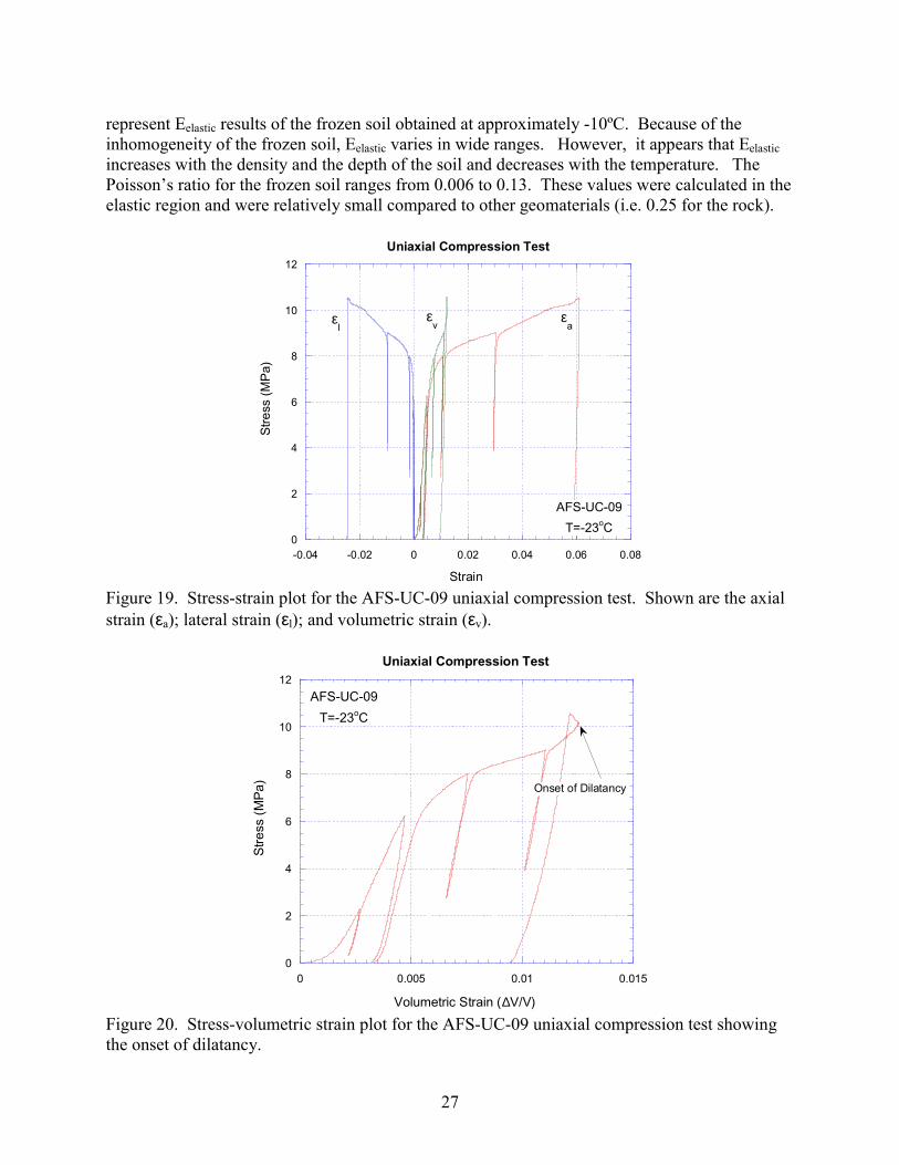
Figure 19. Stress-strain plot for the AFS-UC-09 uniaxial compression test. Shown arethe axial strain (εa); lateral strain (εl); and volumetric strain (εv)………..…….. 27

Figure 20. Stress-volumetric strain plot for the AFS-UC09 uniaxial compression testshowing the onset of dilatancy…………………………………………….……27

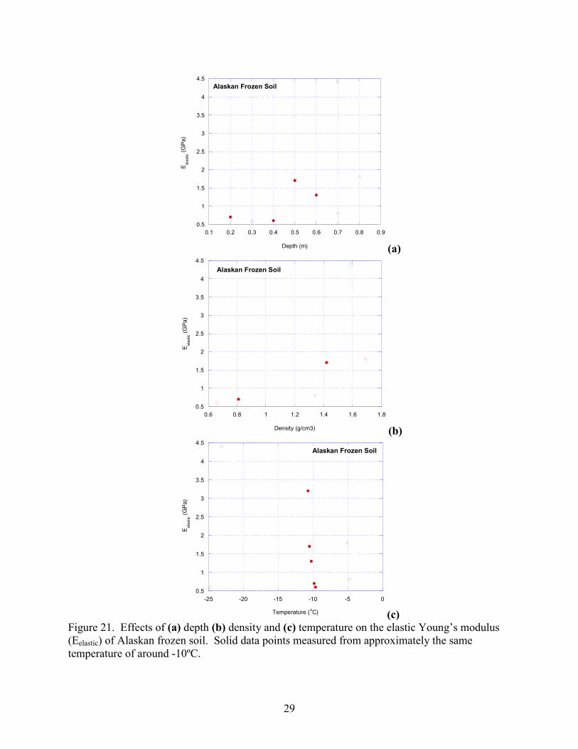
Figure 21. Effects of (a) depth (b) density and (c) temperature on the elastic Young’smodulus (Eelastic) of Alaskan frozen soil. Solid data points measured fromapproximately the same temperature of around -10ºC………………………….29

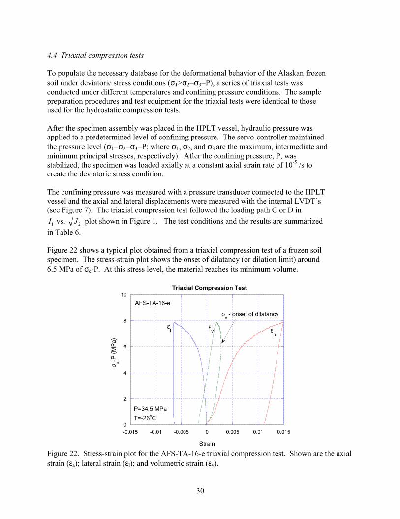
Figure 22. Stress-strain plot for the AFS-TA-16-e triaxial compression test. Shown arethe axial strain (εa); lateral strain (εl); and volumetric strain (εv)………...…… 30

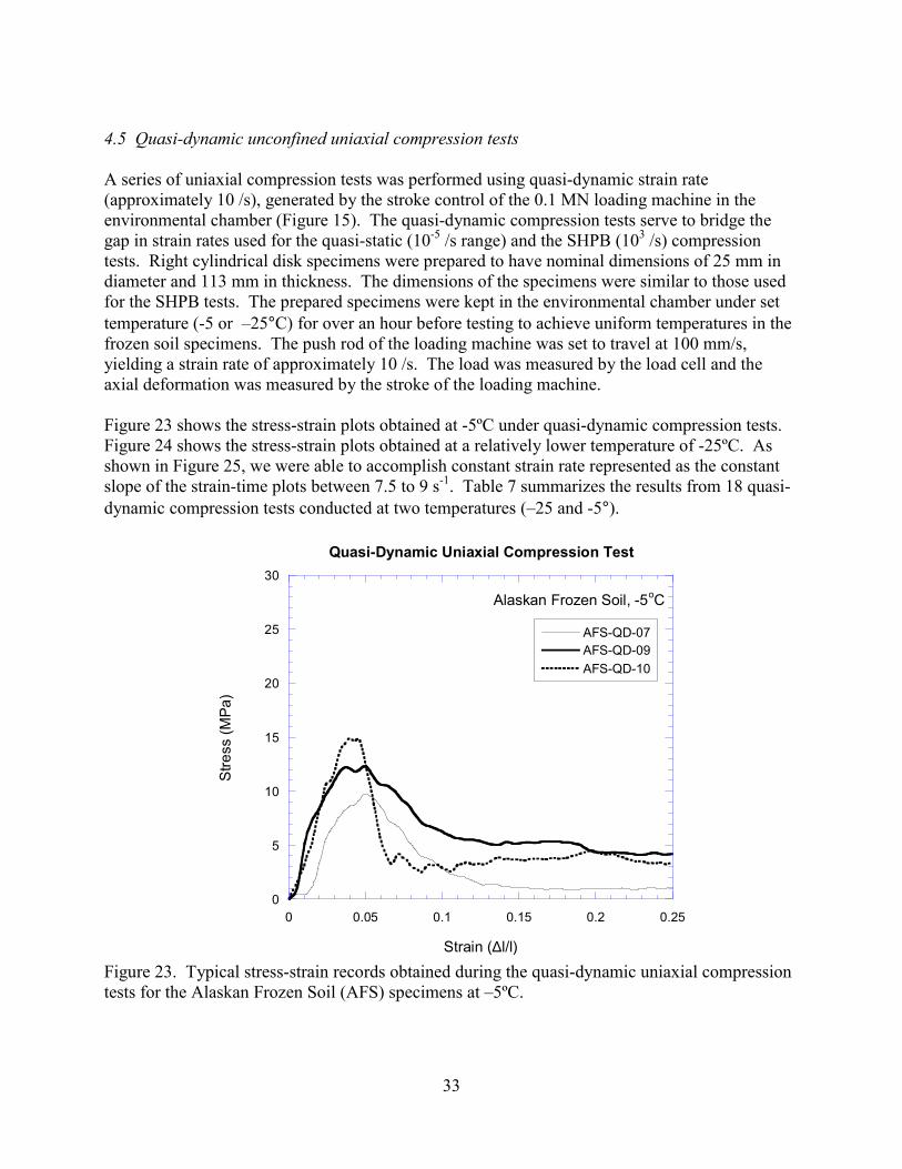
Figure 23. Typical stress-strain records obtained during the quasi-dynamic uniaxialcompression tests for the Alaskan Frozen Soil (AFS) specimens at –5ºC ……. 33

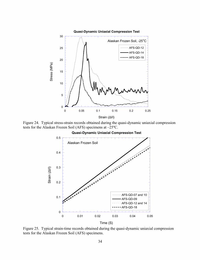
Figure 24. Typical stress-strain records obtained during the quasi-dynamic uniaxialcompression tests for the Alaskan Frozen Soil (AFS) specimens at –25ºC.…... 34

Figure 25. Typical strain-time records obtained during the quasi-dynamic uniaxialcompression tests for the Alaskan Frozen Soil (AFS) specimens……………... 34

Figure 26. Effects of density on (a) the uniaxial compressive strength (C0) and (b) theYoung’s modulus (E) of Alaskan frozen soil………………………………..… 36

6

Figure 27. Effects of temperature on (a) the uniaxial compressive strength (C0) and (b)the Young’s modulus (E) of Alaskan frozen soil……………………………… 37

Figure 28. Schematic of the SHPB system used for testing Alaskan frozen soil……….… 38

Figure 29. The SHPB testing system used for testing Alaskan frozen soil……………….. 39

Figure 30. Felt metal disk, approximately 1 cm in diameter and 0.2 cm in thickness, usedas a pulse shaper……………………………………………………………….. 41

Figure 31. Typical strain-time record obtained during SHPB testing of an Alaskan frozensoil specimen……………………………………………………………………41

Figure 32. Typical stress-time and strain rate-time record obtained during SHPB testingof an Alaskan frozen soil specimen………………………………………...….. 42

Figure 33. Typical stress-strain plot obtained from SHPB testing of an Alaskan frozensoil specimen……………………………………………………..………….... 42

Figure 34. Variations of the strength of the Alaskan frozen soil with respect to density atdifferent temperatures: (a) at -5°C (b) at -10°C and (c) at -25°C…………..… 44

Figure 35. Variations of the Young’s Modulus of the Alaskan frozen soil with respect todensity at different temperatures: (a) at -5°C (b) at -10°C and (c) at -25°C..… 45

Figure 36. Strength of the Alaskan frozen soil plotted against strain rate at two differenttemperatures. Trade-offs between the temperature and strain rate wereobserved for the strength of the Alaskan frozen soil…………………………... 50

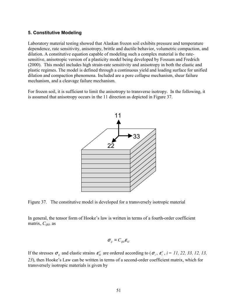
Figure 37. The constitutive model is developed for a transversely isotropic material….… 51

Figure 38. Alaskan frozen soil model versus measured brittle shear-failure data…….….. 54

Figure 39. Alaskan frozen soil model versus measured isotropic hydrostatic compressiondata………………………………………………………………………….…..54

Figure 40. Alaskan frozen soil model versus measured isotropic triaxial compressiondata…………………………………………………………………………..….55

Figure 41. Yield surface and load path followed during a triaxial compression test…..…..56

Figure 42. Comparison of a high-rate model calculation with a quasi-static modelcalculation and a split Hopkinson bar experimental result………………….…. 56

Figure 43. Approximated strain rate used for model calculation…………………………..57

7

Figure 44. Alaskan frozen soil model versus measured quasi-static anisotropichydrostatic compression data…………………………………………………...57

Tables

Table 1. Planned test matrix for the laboratory constitutive testing of Alaskan frozen soil.………………………………………………………………………………….... 9

Table 2. Variations of water content with respect to depth in the Alaskan frozen soil…… 12

Table 3. Summary of hydrostatic compression tests of Alaskan frozen soil……………... 20

Table 4. Summary of Brazilian tensile tests of Alaskan frozen soil under two differenttemperature conditions……………………………………………………………25

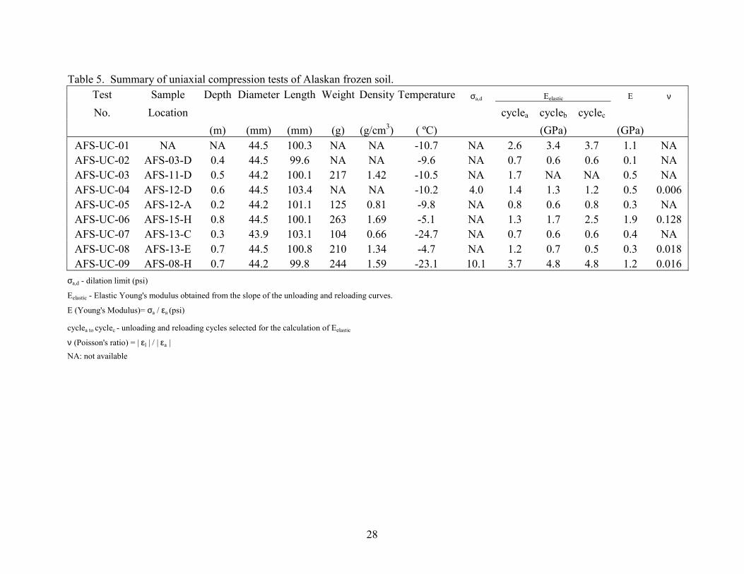
Table 5. Summary of uniaxial compression tests of Alaskan frozen soil……………….....28

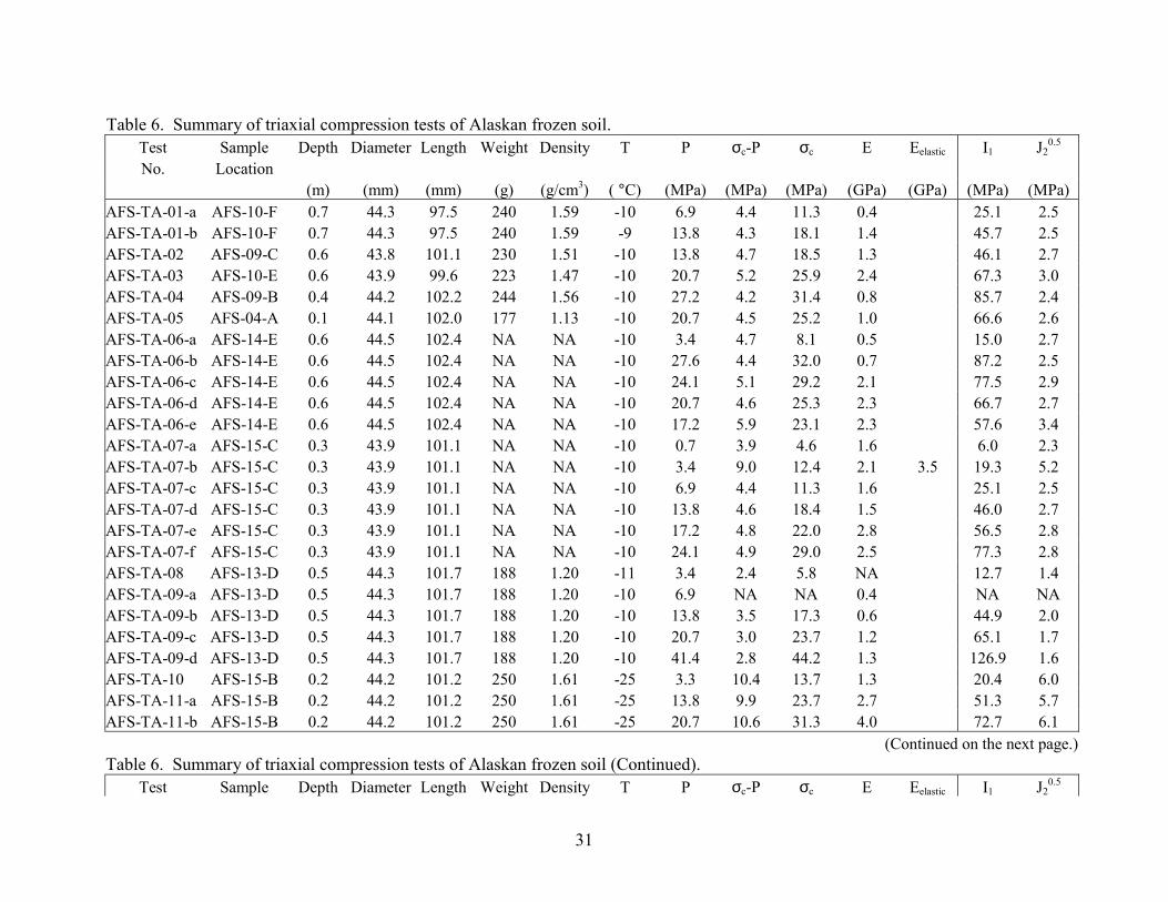
Table 6. Summary of triaxial compression tests of Alaskan frozen soil………………..… 31

Table 7. Summary of quasi-dynamic uniaxial compression tests of Alaskan frozen soil… 35

Table 8. Summary of split Hopkinson pressure bar tests of Alaskan frozen soil…...…….. 46

Table A-1. List of Windows Meta Files (*.wmf) archived in the supplemental CD………62

Table A-2. List of KaleidaGraph (http://www.synergy.com) Files (*.qpc) archived in thesupplemental CD.…….………………………… ………………………….…..63

8

1. Introduction

The current computational model for projectile penetration into frozen soil includes a realisticand general rock and soil materials model (Fossum and Fredrich, 2000). This model is ananisotropic, continuous, three-invariant, single-surface dilation/compaction plasticity model withmixed hardening and limit-state weakening. It is envisioned that this model will be used topredict the deformation and failure of frozen soil under the static and dynamic loading conditionsresulting from projectile penetration. To predict the behavior of the frozen soil based on themodel calculation, the necessary material constants must be estimated from a database populatedfrom laboratory tests, conducted at the requisite conditions on frozen soil specimens.

However, there is little understanding of the mechanics of penetration of frozen soil that areinhomogeneous, highly variable on almost any scale and have large uncertainties associated withbasic material properties. Moreover, only sparse data are available from triaxial compressionexperiments (Gratz and Schulson, 1996; Chamberlain et. al, 1972) conducted at the ColdRegions Research and Engineering Laboratory (CRREL) and Dartmouth College, on artificialfrozen soil samples and on frozen soil obtained from the Yukon Range at Fort Wainwright,Alaska.

The objective of this project was to establish a well-determined set of constitutive data fromquasi-static, quasi-dynamic, and dynamic tests on Alaskan frozen soil. These tests were to beconducted using the unique high-pressure, low-temperature apparatus (Zeuch et. al, 1999) andthe split Hopkinson pressure bar (SHPB).

To estimate the material properties for implementation and validation, several types of quasi-static and dynamic SHPB tests were required. Quasi-static compression tests and indirecttension (or Brazilian) tests, were required to constrain the variabilities of material properties offrozen soil. The SHPB tests were required to obtain dynamic compression properties and thestrain rate dependency of the frozen soil. The experimental program for the Alaskan frozen soilis composed of:

• A suite of quasi-static hydrostatic compression tests to determine the elastic bulkmodulus, K, and the isotropic hardening parameters.

• A set of quasi-static triaxial compression tests to determine the shear modulus, shearfailure properties, and yield surface shape.

• A series of Brazilian tests to determine the appropriate tension cut-off.• A series of SHPB experiments. Deformation of the Alaskan frozen soil at strain rates up

to 103 /s was evaluated at different temperatures. It was postulated that because of thenature of the deformation mechanisms in frozen soils, there would be a direct relationshipbetween the effect of temperature and strain rate on the behavior of the soil. If the trade-off relationship between the temperature and strain rate is established, the behavior offrozen soil under dynamic loading conditions should be well understood by quasi-statictests conducted at a lower temperature.

• A series of quasi-dynamic loading tests that will bridge the gap in loading rates used forthe quasi-static triaxial test at 10-5 /s and the SHPB experiments up to 103 /s.

9

Table 1. Planned test matrix for the laboratory constitutive testing of Alaskan frozen soil.Test Type Temperature

(° C)No. of

Tests PlannedLoading

PathTest Control

Hydrostaticcompression

-25° C 5 A Pressure control0.03 MPa/s

Uniaxialcompression

-25° C-10° C

5 B Strain control10-4 to 10-1

Deviatoriccompression

-25° C 20 C, D Strain control10-4

Indirect tension(Brazilian)

-25° C-10° C

20 E Stroke control10-3 mm/s

Split Hopkinsonbar testing

-25° C-10° C

20 B Up to 103 /sstrain rate

Quasi-dynamiccompression

-25° C-10° C

10 B Up to 10 /sstrain rate

I1

D

A

E

B C

2J

Figure 1. Summary of loading paths used for laboratory testing of frozen soil for constitutivemodeling. I1 is the first invariant of the Cauchy stress tensor and J2 is the second invariant of thedeviatoric stress tensor. Two invariants are defined as I1 = σ1+σ2+σ3 and J2={(σ1 - σ2)2 + (σ2 -

σ3)2 + ( σ3 - σ1)2} / 6 where σ1, σ2 and σ3 are the maximum, intermediate and minimum principalcompressive stresses, respectively.

10

The experimental matrix shown in Table 1 and Figure 1 was used to construct the constitutivedatabase for the frozen soil at confining pressures up to 100 MPa and temperatures down to–25°C. Once a data set with sufficient information is constructed, an assessment can be made ofthe adequacy of the material model to represent the deformation of frozen soil under penetratingprojectile conditions. The data, along with a suitable numerical constitutive model, are critical inpredicting the behavior of penetrator weapons into frozen soil targets.

2. Sample Preparation and Characterization

2.1 Sample preparation

The frozen soil cores were extracted from FTU-11-18 and FTU-11-24 sites in the Yukon TestRange at Eielson Air Force Base in Alaska. The US Army Cold Regions Research andEngineering Laboratory conducted sampling activities using a 7.6 cm diameter coring auger kitdeveloped by CREEL (Ueda et. al, 1975). The coring auger was specially designed for samplingundisturbed fine-grained frozen soils near the earth’s surface in the cold regions. The extractedcores were shipped in a cooler to Sandia National Laboratories and stored in a freezer at–10° C. The diameter of the core was 7.6 cm and the length of the core measured from thesurface was approximately 80 cm.

A water-jet cutting technique was used to extract smaller diameter core specimens from the 7.6cm core. Initially, a drill bit, cooled by liquid nitrogen, was used. However, the drill bit showeda tendency to get jammed when used in fine-grained frozen soils because of lost circulation ofcoolant and accumulation of soil cuttings around the bit. Consequently, it was impossible toextract undisturbed small diameter core specimens. The water-jet cuts the specimen using thestream of high pressure (approximately 400 MPa) water, mixed with abrasives exiting the smalldiameter nozzle. We used the nozzle with 0.03 cm orifice in diameter. The narrow stream of thewater-jet creates fewer disturbances to the specimens than drilling with a core barrel.

Figure 2. Water-jet cutting of cylindrical specimen from the frozen soil core.

11

Figure 2 shows water jet coring used for preparing a cylindrical specimen from frozen soil cores.The extracted specimen was then cut perpendicular to the longitudinal axis of the core, using adiamond saw cooled by liquid nitrogen.

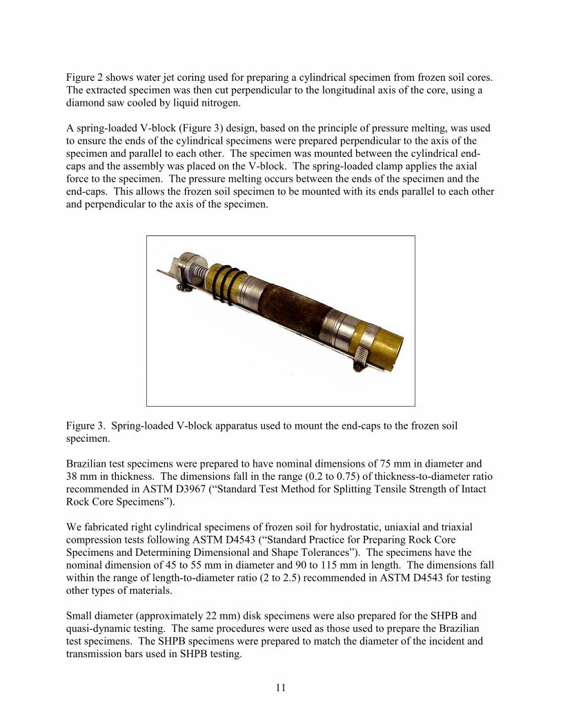
A spring-loaded V-block (Figure 3) design, based on the principle of pressure melting, was usedto ensure the ends of the cylindrical specimens were prepared perpendicular to the axis of thespecimen and parallel to each other. The specimen was mounted between the cylindrical end-caps and the assembly was placed on the V-block. The spring-loaded clamp applies the axialforce to the specimen. The pressure melting occurs between the ends of the specimen and theend-caps. This allows the frozen soil specimen to be mounted with its ends parallel to each otherand perpendicular to the axis of the specimen.

Figure 3. Spring-loaded V-block apparatus used to mount the end-caps to the frozen soilspecimen.

Brazilian test specimens were prepared to have nominal dimensions of 75 mm in diameter and38 mm in thickness. The dimensions fall in the range (0.2 to 0.75) of thickness-to-diameter ratiorecommended in ASTM D3967 (“Standard Test Method for Splitting Tensile Strength of IntactRock Core Specimens”).

We fabricated right cylindrical specimens of frozen soil for hydrostatic, uniaxial and triaxialcompression tests following ASTM D4543 (“Standard Practice for Preparing Rock CoreSpecimens and Determining Dimensional and Shape Tolerances”). The specimens have thenominal dimension of 45 to 55 mm in diameter and 90 to 115 mm in length. The dimensions fallwithin the range of length-to-diameter ratio (2 to 2.5) recommended in ASTM D4543 for testingother types of materials.

Small diameter (approximately 22 mm) disk specimens were also prepared for the SHPB andquasi-dynamic testing. The same procedures were used as those used to prepare the Braziliantest specimens. The SHPB specimens were prepared to match the diameter of the incident andtransmission bars used in SHPB testing.

12

2.2 Sample characterization

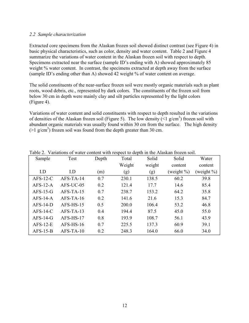
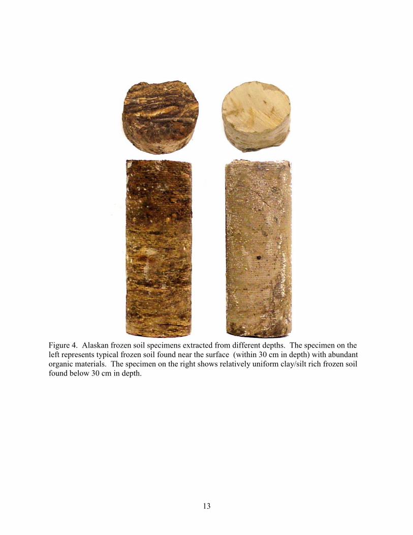
Extracted core specimens from the Alaskan frozen soil showed distinct contrast (see Figure 4) inbasic physical characteristics, such as color, density and water content. Table 2 and Figure 4summarize the variations of water content in the Alaskan frozen soil with respect to depth.Specimens extracted near the surface (sample ID’s ending with A) showed approximately 85weight % water content. In contrast, the specimens extracted at depth away from the surface(sample ID’s ending other than A) showed 42 weight % of water content on average.

The solid constituents of the near-surface frozen soil were mostly organic materials such as plantroots, wood debris, etc., represented by dark colors. The constituents of the frozen soil frombelow 30 cm in depth were mainly clay and silt particles represented by the light colors(Figure 4).

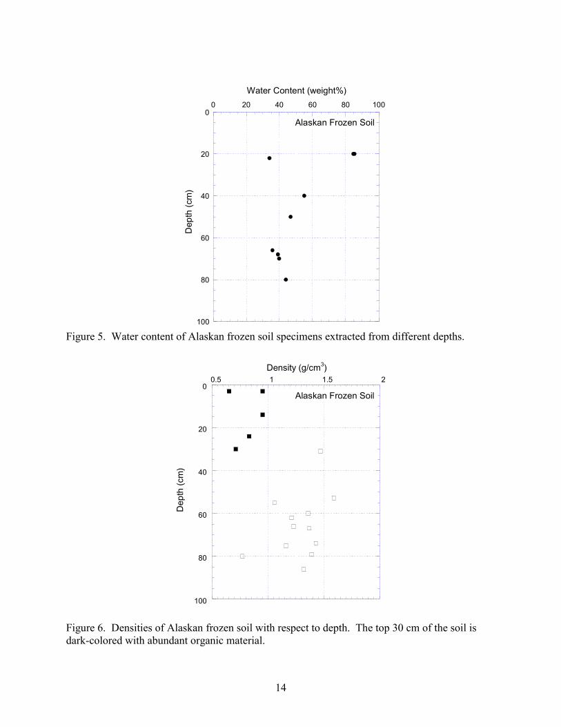
Variations of water content and solid constituents with respect to depth resulted in the variationsof densities of the Alaskan frozen soil (Figure 5). The low density (<1 g/cm3) frozen soil withabundant organic materials was usually found within 30 cm from the surface. The high density(>1 g/cm3) frozen soil was found from the depth greater than 30 cm.

Table 2. Variations of water content with respect to depth in the Alaskan frozen soil.Sample Test Depth Total Solid Solid Water

Weight weight content contentI.D I.D (m) (g) (g) (weight %) (weight %)

AFS-12-C AFS-TA-14 0.7 230.1 138.5 60.2 39.8AFS-12-A AFS-UC-05 0.2 121.4 17.7 14.6 85.4AFS-15-G AFS-TA-15 0.7 238.7 153.2 64.2 35.8AFS-14-A AFS-TA-16 0.2 141.6 21.6 15.3 84.7AFS-14-D AFS-HS-15 0.5 200.0 106.4 53.2 46.8AFS-14-C AFS-TA-13 0.4 194.4 87.5 45.0 55.0AFS-14-G AFS-HS-17 0.8 193.9 108.7 56.1 43.9AFS-12-E AFS-HS-16 0.7 225.5 137.3 60.9 39.1AFS-15-B AFS-TA-10 0.2 248.3 164.0 66.0 34.0

13

Figure 4. Alaskan frozen soil specimens extracted from different depths. The specimen on theleft represents typical frozen soil found near the surface (within 30 cm in depth) with abundantorganic materials. The specimen on the right shows relatively uniform clay/silt rich frozen soilfound below 30 cm in depth.

14

0 20 40 60 80 1000

20

40

60

80

100

Water Content (weight%)

Dep

th (c

m)

Alaskan Frozen Soil

Figure 5. Water content of Alaskan frozen soil specimens extracted from different depths.

0.5 1 1.5 20

20

40

60

80

100

Density (g/cm3)

Dep

th (c

m)

Alaskan Frozen Soil

Figure 6. Densities of Alaskan frozen soil with respect to depth. The top 30 cm of the soil isdark-colored with abundant organic material.

15

3. Development of High-Pressure Low-Temperature (HPLT) Triaxial Test Cell

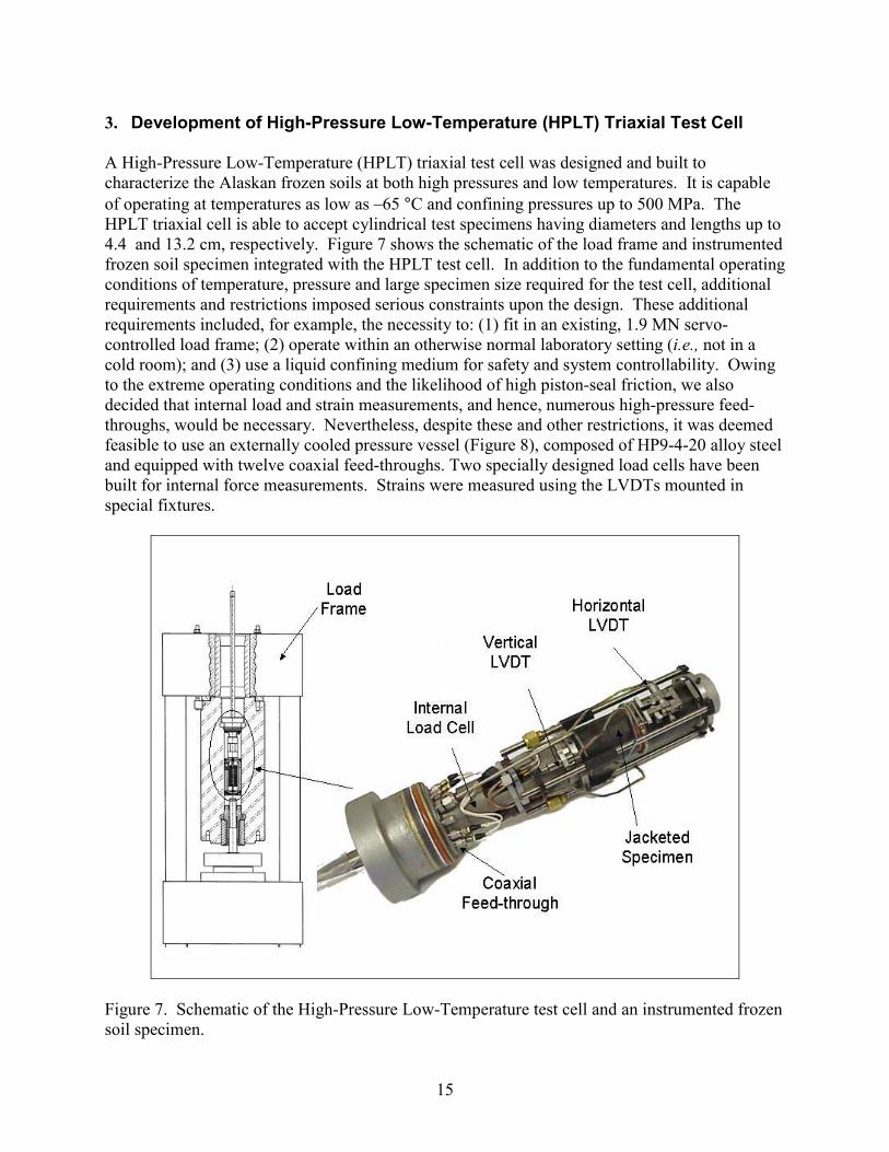
A High-Pressure Low-Temperature (HPLT) triaxial test cell was designed and built tocharacterize the Alaskan frozen soils at both high pressures and low temperatures. It is capableof operating at temperatures as low as –65 °C and confining pressures up to 500 MPa. TheHPLT triaxial cell is able to accept cylindrical test specimens having diameters and lengths up to4.4 and 13.2 cm, respectively. Figure 7 shows the schematic of the load frame and instrumentedfrozen soil specimen integrated with the HPLT test cell. In addition to the fundamental operatingconditions of temperature, pressure and large specimen size required for the test cell, additionalrequirements and restrictions imposed serious constraints upon the design. These additionalrequirements included, for example, the necessity to: (1) fit in an existing, 1.9 MN servo-controlled load frame; (2) operate within an otherwise normal laboratory setting (i.e., not in acold room); and (3) use a liquid confining medium for safety and system controllability. Owingto the extreme operating conditions and the likelihood of high piston-seal friction, we alsodecided that internal load and strain measurements, and hence, numerous high-pressure feed-throughs, would be necessary. Nevertheless, despite these and other restrictions, it was deemedfeasible to use an externally cooled pressure vessel (Figure 8), composed of HP9-4-20 alloy steeland equipped with twelve coaxial feed-throughs. Two specially designed load cells have beenbuilt for internal force measurements. Strains were measured using the LVDTs mounted inspecial fixtures.

Figure 7. Schematic of the High-Pressure Low-Temperature test cell and an instrumented frozensoil specimen.

16

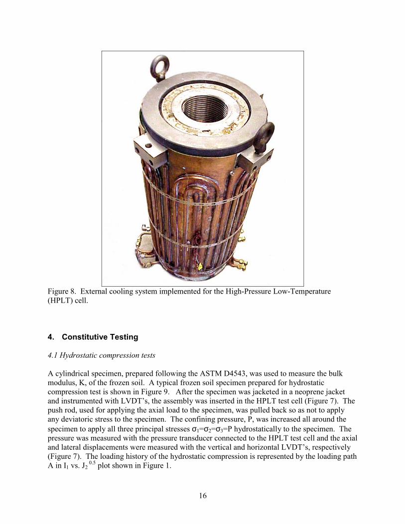
Figure 8. External cooling system implemented for the High-Pressure Low-Temperature(HPLT) cell.

4. Constitutive Testing

4.1 Hydrostatic compression tests

A cylindrical specimen, prepared following the ASTM D4543, was used to measure the bulkmodulus, K, of the frozen soil. A typical frozen soil specimen prepared for hydrostaticcompression test is shown in Figure 9. After the specimen was jacketed in a neoprene jacketand instrumented with LVDT’s, the assembly was inserted in the HPLT test cell (Figure 7). Thepush rod, used for applying the axial load to the specimen, was pulled back so as not to applyany deviatoric stress to the specimen. The confining pressure, P, was increased all around thespecimen to apply all three principal stresses σ1=σ2=σ3=P hydrostatically to the specimen. Thepressure was measured with the pressure transducer connected to the HPLT test cell and the axialand lateral displacements were measured with the vertical and horizontal LVDT’s, respectively(Figure 7). The loading history of the hydrostatic compression is represented by the loading pathA in I1 vs. J2

0.5 plot shown in Figure 1.

17

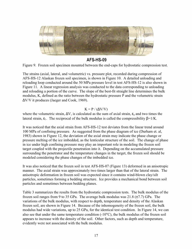
Figure 9. Frozen soil specimen mounted between the end-caps for hydrostatic compression test.

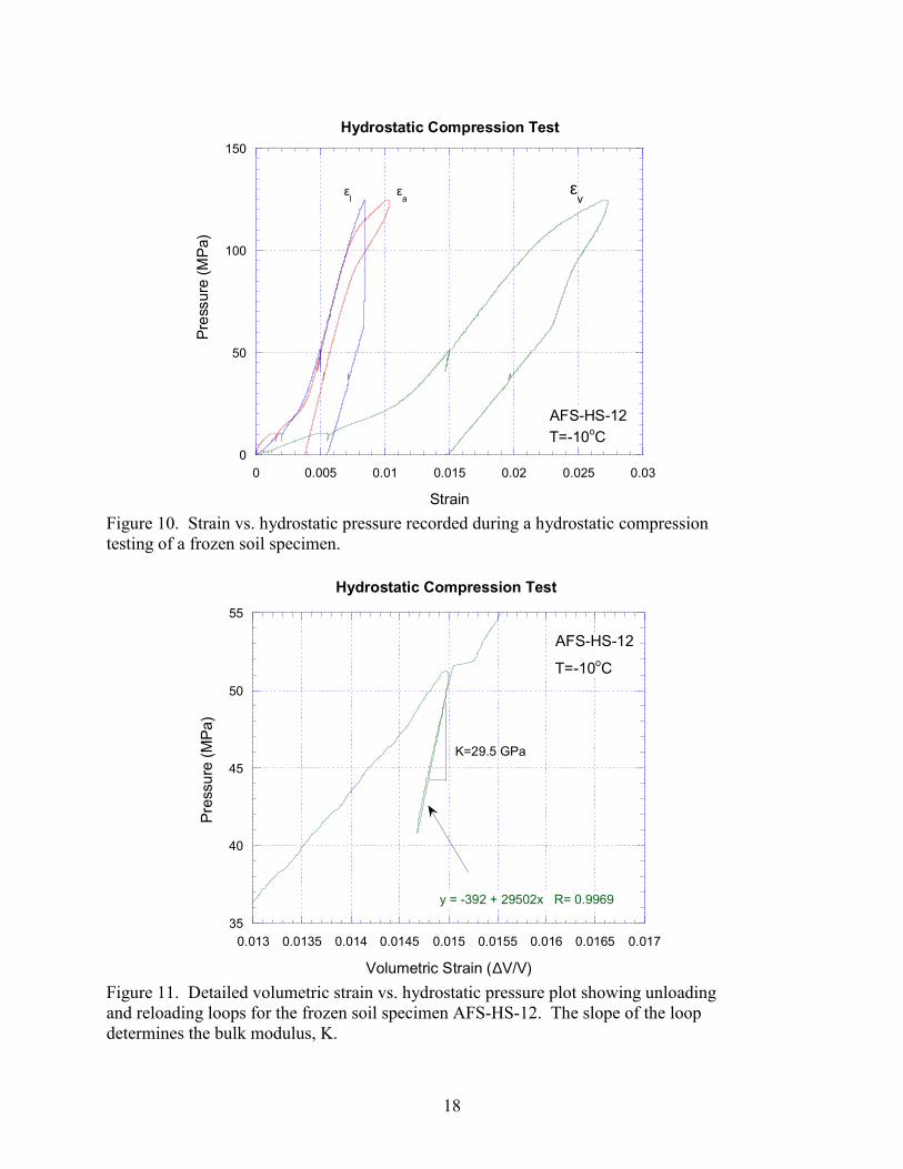
The strains (axial, lateral, and volumetric) vs. pressure plot, recorded during compression ofAFS-HS-12 Alaskan frozen soil specimen, is shown in Figure 10. A detailed unloading andreloading loop conducted around the 50 MPa pressure level in test AFS-HS-12 is also shown inFigure 11. A linear regression analysis was conducted to the data corresponding to unloadingand reloading a portion of the curve. The slope of the best-fit straight line determines the bulkmodulus, K, defined as the ratio between the hydrostatic pressure P and the volumetric strain∆V/V it produces (Jaeger and Cook, 1969).

K = P / (∆V/V)where the volumetric strain, ∆V, is calculated as the sum of axial strain, εa and two times thelateral strain, εl . The reciprocal of the bulk modulus is called the compressibility β=1/K.

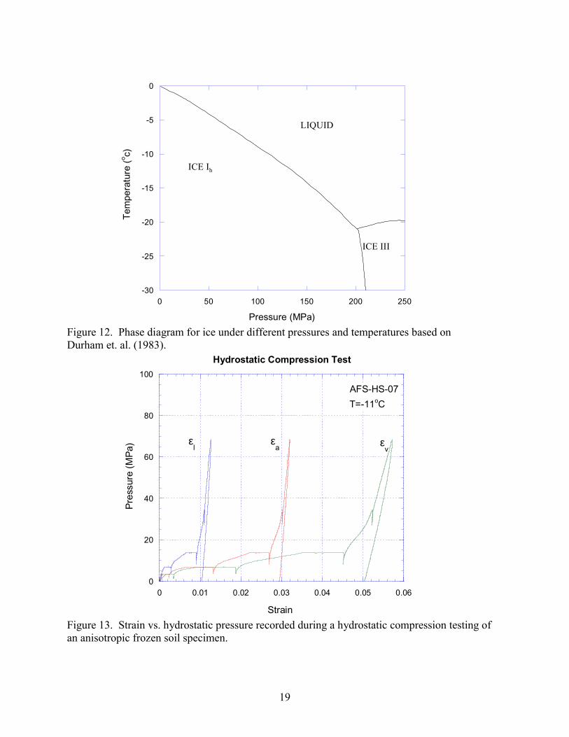
It was noticed that the axial strain from AFS-HS-12 test deviates from the linear trend around100 MPa of confining pressure. As suggested from the phase diagram of ice (Durham et. al,1983) shown in Figure 12, the deviation of the axial strain may indicate the phase change orpressure melting of the ice imbedded, as the lenticular structure of the soil. The change of phasein ice under high confining pressure may play an important role in modeling the frozen soiltarget coupled with the projectile penetration into it. Depending on the accumulated pressuresurrounding the penetrator and the temperature changes in the target, the frozen soil should bemodeled considering the phase changes of the imbedded ice.

It was also noticed that the frozen soil in test AFS-HS-07 (Figure 13) deformed in an anisotropicmanner. The axial strain was approximately two times larger than that of the lateral strain. Theanisotropic deformation in frozen soil was expected since it contains wind-blown clay/siltparticles, sometimes forming a bedding structure. Ice provides a mechanical bond between soilparticles and sometimes between bedding planes.

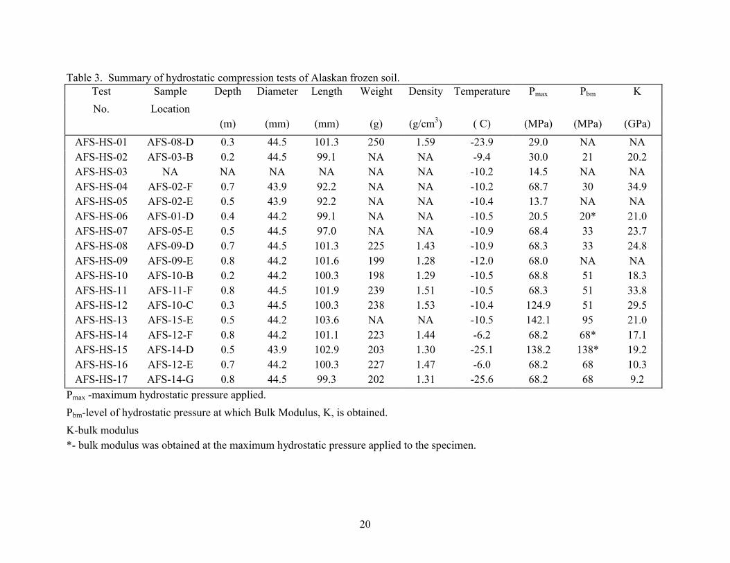
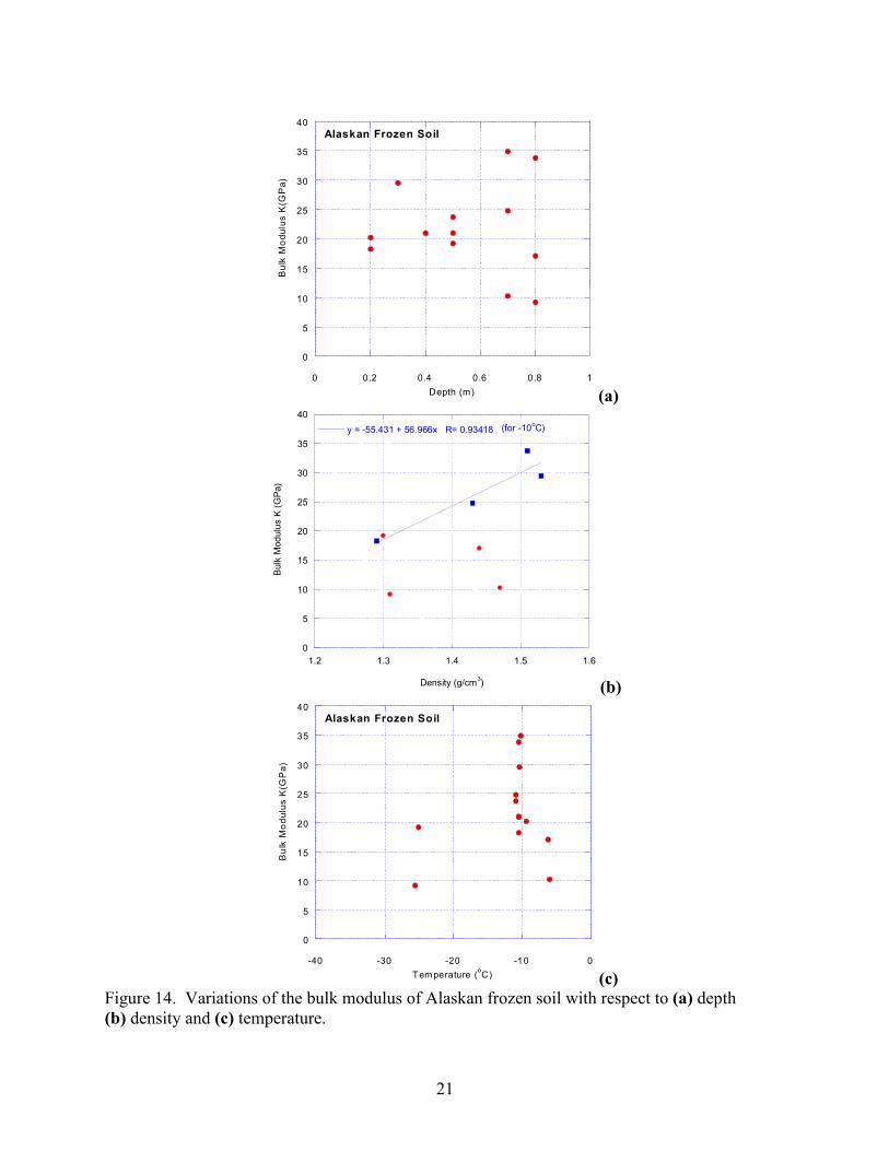
Table 3 summarizes the results from the hydrostatic compression tests. The bulk modulus of thefrozen soil ranges from 9 to 35 GPa. The average bulk modulus was 21.8 (±7.7) GPa. Thevariations of the bulk modulus, with respect to depth, temperature and density of the Alaskanfrozen soil, are shown in Figure 14. Because of the inhomogeneity of the frozen soil, the bulkmodulus had wide variations, up to 25 GPa, for the identical test condition. In Figure 14, we canalso see that under the same temperature condition (-10°C), the bulk modulus of the frozen soilappears to increase with the density of the soil. Other factors, such as depth and temperature,evidently were not associated with the bulk modulus.

18

0

50

100

150

0 0.005 0.01 0.015 0.02 0.025 0.03

AFS-HS-12

Pres

sure

(MPa

)

Strain

εa

εvε

l

Hydrostatic Compression Test

T=-10oC

Figure 10. Strain vs. hydrostatic pressure recorded during a hydrostatic compressiontesting of a frozen soil specimen.

35

40

45

50

55

0.013 0.0135 0.014 0.0145 0.015 0.0155 0.016 0.0165 0.017

AFS-HS-12

Pres

sure

(MPa

)

Volumetric Strain (∆V/V)

y = -392 + 29502x R= 0.9969

K=29.5 GPa


T=-10oC

Figure 11. Detailed volumetric strain vs. hydrostatic pressure plot showing unloadingand reloading loops for the frozen soil specimen AFS-HS-12. The slope of the loopdetermines the bulk modulus, K.

19

-30

-25

-20

-15

-10

-5

0

0 50 100 150 200 250

Tem

pera

ture

(o c)

Pressure (MPa)

LIQUID

ICE Ih

ICE III

Figure 12. Phase diagram for ice under different pressures and temperatures based onDurham et. al. (1983).

0

20

40

60

80

100

0 0.01 0.02 0.03 0.04 0.05 0.06

AFS-HS-07

Pres

sure

(MPa

)

Strain

εa ε

vε

l


T=-11oC

Figure 13. Strain vs. hydrostatic pressure recorded during a hydrostatic compression testing ofan anisotropic frozen soil specimen.

20

Table 3. Summary of hydrostatic compression tests of Alaskan frozen soil.Test Sample Depth Diameter Length Weight Density Temperature Pmax Pbm KNo. Location

(m) (mm) (mm) (g) (g/cm3) ( C) (MPa) (MPa) (GPa)

AFS-HS-01 AFS-08-D 0.3 44.5 101.3 250 1.59 -23.9 29.0 NA NAAFS-HS-02 AFS-03-B 0.2 44.5 99.1 NA NA -9.4 30.0 21 20.2AFS-HS-03 NA NA NA NA NA NA -10.2 14.5 NA NAAFS-HS-04 AFS-02-F 0.7 43.9 92.2 NA NA -10.2 68.7 30 34.9AFS-HS-05 AFS-02-E 0.5 43.9 92.2 NA NA -10.4 13.7 NA NAAFS-HS-06 AFS-01-D 0.4 44.2 99.1 NA NA -10.5 20.5 20* 21.0AFS-HS-07 AFS-05-E 0.5 44.5 97.0 NA NA -10.9 68.4 33 23.7AFS-HS-08 AFS-09-D 0.7 44.5 101.3 225 1.43 -10.9 68.3 33 24.8AFS-HS-09 AFS-09-E 0.8 44.2 101.6 199 1.28 -12.0 68.0 NA NAAFS-HS-10 AFS-10-B 0.2 44.2 100.3 198 1.29 -10.5 68.8 51 18.3AFS-HS-11 AFS-11-F 0.8 44.5 101.9 239 1.51 -10.5 68.3 51 33.8AFS-HS-12 AFS-10-C 0.3 44.5 100.3 238 1.53 -10.4 124.9 51 29.5AFS-HS-13 AFS-15-E 0.5 44.2 103.6 NA NA -10.5 142.1 95 21.0AFS-HS-14 AFS-12-F 0.8 44.2 101.1 223 1.44 -6.2 68.2 68* 17.1AFS-HS-15 AFS-14-D 0.5 43.9 102.9 203 1.30 -25.1 138.2 138* 19.2AFS-HS-16 AFS-12-E 0.7 44.2 100.3 227 1.47 -6.0 68.2 68 10.3AFS-HS-17 AFS-14-G 0.8 44.5 99.3 202 1.31 -25.6 68.2 68 9.2

Pmax -maximum hydrostatic pressure applied.Pbm-level of hydrostatic pressure at which Bulk Modulus, K, is obtained.K-bulk modulus*- bulk modulus was obtained at the maximum hydrostatic pressure applied to the specimen.

21

0

5

10

15

20

25

30

35

40

0 0.2 0.4 0.6 0.8 1

Alaskan Frozen Soil

Bul

k M

odul

us K

(GP

a)

Depth (m) (a)

0

5

10

15

20

25

30

35

40

1.2 1.3 1.4 1.5 1.6

y = -55.431 + 56.966x R= 0.93418

Bulk

Mod

ulus

K (G

Pa)

Density (g/cm3)

(for -10oC)

(b)

0

5

10

15

20

25

30

35

40

-40 -30 -20 -10 0

Alaskan Frozen Soil

Bul

k M

odul

us K

(GP

a)

Temperature (oC) (c)Figure 14. Variations of the bulk modulus of Alaskan frozen soil with respect to (a) depth(b) density and (c) temperature.

22

4.2 Brazilian tests

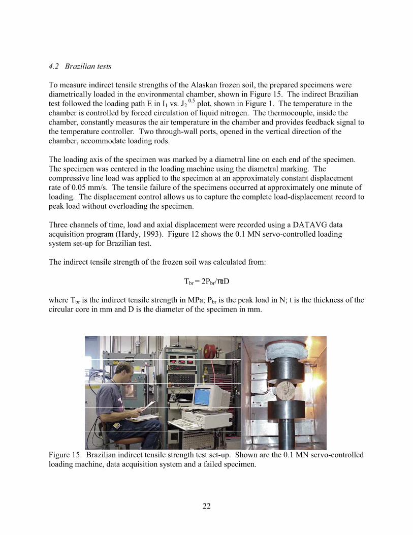
To measure indirect tensile strengths of the Alaskan frozen soil, the prepared specimens werediametrically loaded in the environmental chamber, shown in Figure 15. The indirect Braziliantest followed the loading path E in I1 vs. J2

0.5 plot, shown in Figure 1. The temperature in thechamber is controlled by forced circulation of liquid nitrogen. The thermocouple, inside thechamber, constantly measures the air temperature in the chamber and provides feedback signal tothe temperature controller. Two through-wall ports, opened in the vertical direction of thechamber, accommodate loading rods.

The loading axis of the specimen was marked by a diametral line on each end of the specimen.The specimen was centered in the loading machine using the diametral marking. Thecompressive line load was applied to the specimen at an approximately constant displacementrate of 0.05 mm/s. The tensile failure of the specimens occurred at approximately one minute ofloading. The displacement control allows us to capture the complete load-displacement record topeak load without overloading the specimen.

Three channels of time, load and axial displacement were recorded using a DATAVG dataacquisition program (Hardy, 1993). Figure 12 shows the 0.1 MN servo-controlled loadingsystem set-up for Brazilian test.

The indirect tensile strength of the frozen soil was calculated from:

Tbr = 2Pbr/πtD

where Tbr is the indirect tensile strength in MPa; Pbr is the peak load in N; t is the thickness of thecircular core in mm and D is the diameter of the specimen in mm.

Figure 15. Brazilian indirect tensile strength test set-up. Shown are the 0.1 MN servo-controlledloading machine, data acquisition system and a failed specimen.

23

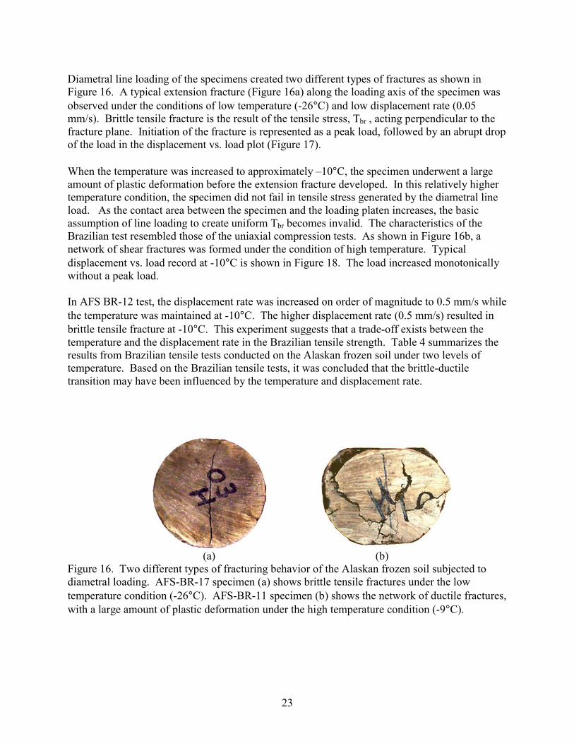
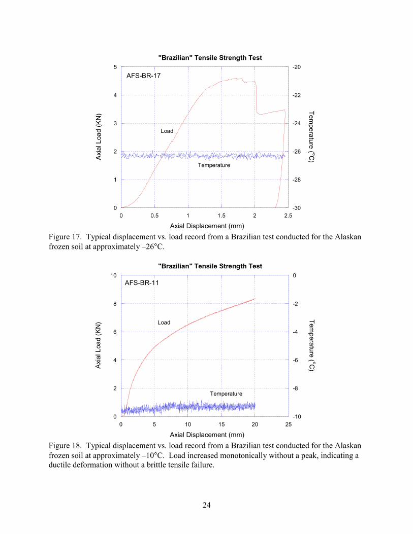
Diametral line loading of the specimens created two different types of fractures as shown inFigure 16. A typical extension fracture (Figure 16a) along the loading axis of the specimen wasobserved under the conditions of low temperature (-26°C) and low displacement rate (0.05mm/s). Brittle tensile fracture is the result of the tensile stress, Tbr , acting perpendicular to thefracture plane. Initiation of the fracture is represented as a peak load, followed by an abrupt dropof the load in the displacement vs. load plot (Figure 17).

When the temperature was increased to approximately –10°C, the specimen underwent a largeamount of plastic deformation before the extension fracture developed. In this relatively highertemperature condition, the specimen did not fail in tensile stress generated by the diametral lineload. As the contact area between the specimen and the loading platen increases, the basicassumption of line loading to create uniform Tbr becomes invalid. The characteristics of theBrazilian test resembled those of the uniaxial compression tests. As shown in Figure 16b, anetwork of shear fractures was formed under the condition of high temperature. Typicaldisplacement vs. load record at -10°C is shown in Figure 18. The load increased monotonicallywithout a peak load.

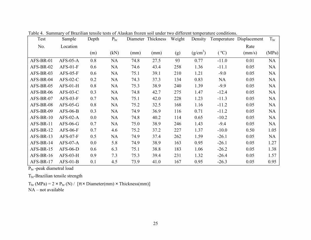
In AFS BR-12 test, the displacement rate was increased on order of magnitude to 0.5 mm/s whilethe temperature was maintained at -10°C. The higher displacement rate (0.5 mm/s) resulted inbrittle tensile fracture at -10°C. This experiment suggests that a trade-off exists between thetemperature and the displacement rate in the Brazilian tensile strength. Table 4 summarizes theresults from Brazilian tensile tests conducted on the Alaskan frozen soil under two levels oftemperature. Based on the Brazilian tensile tests, it was concluded that the brittle-ductiletransition may have been influenced by the temperature and displacement rate.

(a) (b)Figure 16. Two different types of fracturing behavior of the Alaskan frozen soil subjected todiametral loading. AFS-BR-17 specimen (a) shows brittle tensile fractures under the lowtemperature condition (-26°C). AFS-BR-11 specimen (b) shows the network of ductile fractures,with a large amount of plastic deformation under the high temperature condition (-9°C).

24

0

1

2

3

4

5

-30

-28

-26

-24

-22

-20

0 0.5 1 1.5 2 2.5

"Brazilian" Tensile Strength Test

Axi

al L

oad

(KN

)Tem

perature ( oC)

Axial Displacement (mm)

Temperature

Load

AFS-BR-17

Figure 17. Typical displacement vs. load record from a Brazilian test conducted for the Alaskanfrozen soil at approximately –26°C.

0

2

4

6

8

10

-10

-8

-6

-4

-2

0

0 5 10 15 20 25

"Brazilian" Tensile Strength Test

Axia

l Loa

d (K

N)

Temperature ( oC

)

Axial Displacement (mm)

Temperature

Load

AFS-BR-11

Figure 18. Typical displacement vs. load record from a Brazilian test conducted for the Alaskanfrozen soil at approximately –10°C. Load increased monotonically without a peak, indicating aductile deformation without a brittle tensile failure.

25

Table 4. Summary of Brazilian tensile tests of Alaskan frozen soil under two different temperature conditions.Test Sample Depth Pbr Diameter Thickness Weight Density Temperature Displacement Tbr

No. Location Rate(m) (kN) (mm) (mm) (g) (g/cm3) ( ºC) (mm/s) (MPa)

AFS-BR-01 AFS-05-A 0.8 NA 74.8 27.5 93 0.77 -11.0 0.01 NAAFS-BR-02 AFS-01-F 0.6 NA 74.6 43.4 258 1.36 -11.1 0.05 NAAFS-BR-03 AFS-05-F 0.6 NA 75.1 39.1 210 1.21 -9.0 0.05 NAAFS-BR-04 AFS-02-C 0.2 NA 74.3 37.3 134 0.83 NA 0.05 NAAFS-BR-05 AFS-01-H 0.8 NA 75.3 38.9 240 1.39 -9.9 0.05 NAAFS-BR-06 AFS-03-C 0.3 NA 74.8 42.7 275 1.47 -12.4 0.05 NAAFS-BR-07 AFS-03-F 0.7 NA 75.1 42.0 228 1.23 -11.3 0.05 NAAFS-BR-08 AFS-05-G 0.8 NA 75.2 32.5 168 1.16 -11.2 0.05 NAAFS-BR-09 AFS-06-B 0.3 NA 74.9 36.9 116 0.71 -11.2 0.05 NAAFS-BR-10 AFS-02-A 0.0 NA 74.8 40.2 114 0.65 -10.2 0.05 NAAFS-BR-11 AFS-06-G 0.7 NA 75.0 38.9 246 1.43 -9.4 0.05 NAAFS-BR-12 AFS-06-F 0.7 4.6 75.2 37.2 227 1.37 -10.0 0.50 1.05AFS-BR-13 AFS-07-F 0.5 NA 74.9 37.4 262 1.59 -26.1 0.05 NAAFS-BR-14 AFS-07-A 0.0 5.8 74.9 38.9 163 0.95 -26.1 0.05 1.27AFS-BR-15 AFS-06-D 0.6 6.3 75.1 38.8 183 1.06 -26.2 0.05 1.38AFS-BR-16 AFS-03-H 0.9 7.3 75.3 39.4 231 1.32 -26.4 0.05 1.57AFS-BR-17 AFS-01-B 0.1 4.5 73.9 41.0 167 0.95 -26.3 0.05 0.95

Pbr -peak diametral loadTbr-Brazilian tensile strength

Tbr (MPa) = 2 × Pbr (N) / [π × Diameter(mm) × Thickness(mm)]NA – not available

26

4.3 Unconfined uniaxial compression tests

Uniaxial compression tests were conducted in a 0.1 MN servo-controlled loading machine. Theprepared specimens were loaded at a constant displacement rate of 10-3 mm/s which correspondsto a strain rate of 10-5 /s. The axial and lateral deformations were measured from the axial andthe circumferential LVDT’s, respectively. The instrumented specimen was placed between theupper and lower cylindrical end-caps with the same diameter as the specimen. The specimenswere loaded until 5 to 6% of axial strain was reached. Unlike the brittle failure observed in therock, the frozen soil specimens were deformed in a ductile manner, without the peak stress andsignificant stress drop immediately following it. Therefore, the uniaxial compressive strength ofthe frozen soil was not calculated. Instead of the uniaxial compressive strength, dilatancy wasconsidered to be the measure of damage stress for the frozen soil. The dilatancy, defined as thepoint at which the specimen reaches its minimum volume, was based on the volumetic strain, εv,calculated as follows:

εv= εa + 2εlwhere εa and εl are the axial and lateral strains, respectively.

Based on the volumetric strain data, dilatancy was observed in two uniaxial compression tests:(AFS-UC-04 and AFS-UC-09).

The proportional constant between stress and strain in the elastic portion of compression testsdefines the Young’s modulus:

E = σa / εa

where σa is the axial stress and εa is the axial strain. The Young’s modulus was determined byfitting a straight line (or linear regression analysis) to the stress strain data that ranged fromapproximately 10 to 50% of the peak stress. When approximately 50% of the expected peakload P was reached, unloading and reloading cycles were carried out. The elastic Young’smodulus, Eelastic, due only to the elastic deformation of the specimen, was calculated from theslope of the unloading curve. Linear regression analysis was also used to obtain the best-fitstraight line to the unloading curve.

Also, the ratio between the axial (εa) and lateral (εl) strains is defined as the Poisson’s ratio (ν):

ν = |εl | / |εa|

Nine Alaskan frozen soil specimens were tested to obtain elastic constants, E, Eelastic and ν. Theresults are summarized in Table 5. Figure 19 shows the example of unloading and reloadingcycles for the uniaxial compression test. The onset of dilatancy for the same test is shown inFigure 20.

The variations of Eelastic, with respect to the depth, density and temperature of the Alaskan frozensoil are shown in Figure 21. In order to correlate Eelastic to different test variables, we groupedthe test results, with respect to the set temperature, in the frozen soil. Solid symbols in Figure 21

27

represent Eelastic results of the frozen soil obtained at approximately -10ºC. Because of theinhomogeneity of the frozen soil, Eelastic varies in wide ranges. However, it appears that Eelasticincreases with the density and the depth of the soil and decreases with the temperature. ThePoisson’s ratio for the frozen soil ranges from 0.006 to 0.13. These values were calculated in theelastic region and were relatively small compared to other geomaterials (i.e. 0.25 for the rock).

0

2

4

6

8

10

12

-0.04 -0.02 0 0.02 0.04 0.06 0.08

AFS-UC-09T=-23oC

Stre

ss (M

Pa)

Strain

εa

εvε

l

Uniaxial Compression Test

Figure 19. Stress-strain plot for the AFS-UC-09 uniaxial compression test. Shown are the axialstrain (εa); lateral strain (εl); and volumetric strain (εv).

0

2

4

6

8

10

12

0 0.005 0.01 0.015

AFS-UC-09T=-23oC

Stre

ss (M

Pa)

Volumetric Strain (∆V/V)

Onset of Dilatancy

Uniaxial Compression Test

Figure 20. Stress-volumetric strain plot for the AFS-UC-09 uniaxial compression test showingthe onset of dilatancy.

28

Table 5. Summary of uniaxial compression tests of Alaskan frozen soil.Test Sample Depth Diameter Length Weight Density Temperature σa,d Eelastic E ν

No. Location cyclea cycleb cyclec (m) (mm) (mm) (g) (g/cm3) ( ºC) (GPa) (GPa)

AFS-UC-01 NA NA 44.5 100.3 NA NA -10.7 NA 2.6 3.4 3.7 1.1 NAAFS-UC-02 AFS-03-D 0.4 44.5 99.6 NA NA -9.6 NA 0.7 0.6 0.6 0.1 NAAFS-UC-03 AFS-11-D 0.5 44.2 100.1 217 1.42 -10.5 NA 1.7 NA NA 0.5 NAAFS-UC-04 AFS-12-D 0.6 44.5 103.4 NA NA -10.2 4.0 1.4 1.3 1.2 0.5 0.006AFS-UC-05 AFS-12-A 0.2 44.2 101.1 125 0.81 -9.8 NA 0.8 0.6 0.8 0.3 NAAFS-UC-06 AFS-15-H 0.8 44.5 100.1 263 1.69 -5.1 NA 1.3 1.7 2.5 1.9 0.128AFS-UC-07 AFS-13-C 0.3 43.9 103.1 104 0.66 -24.7 NA 0.7 0.6 0.6 0.4 NAAFS-UC-08 AFS-13-E 0.7 44.5 100.8 210 1.34 -4.7 NA 1.2 0.7 0.5 0.3 0.018AFS-UC-09 AFS-08-H 0.7 44.2 99.8 244 1.59 -23.1 10.1 3.7 4.8 4.8 1.2 0.016

σa,d - dilation limit (psi)

Eelastic - Elastic Young's modulus obtained from the slope of the unloading and reloading curves.

E (Young's Modulus)= σa / εa (psi)

cyclea to cyclec - unloading and reloading cycles selected for the calculation of Eelastic

ν (Poisson's ratio) = | εl | / | εa |NA: not available

29

0.5

1

1.5

2

2.5

3

3.5

4

4.5

0.1 0.2 0.3 0.4 0.5 0.6 0.7 0.8 0.9

E elas

tic (G

Pa)

Depth (m)

Alaskan Frozen Soil

(a)

0.5

1

1.5

2

2.5

3

3.5

4

4.5

0.6 0.8 1 1.2 1.4 1.6 1.8

E elas

tic (G

Pa)

Density (g/cm3)

Alaskan Frozen Soil

(b)

0.5

1

1.5

2

2.5

3

3.5

4

4.5

-25 -20 -15 -10 -5 0

E elas

tic (G

Pa)

Temperature (oC)

Alaskan Frozen Soil

(c)Figure 21. Effects of (a) depth (b) density and (c) temperature on the elastic Young’s modulus(Eelastic) of Alaskan frozen soil. Solid data points measured from approximately the sametemperature of around -10ºC.

30

4.4 Triaxial compression tests

To populate the necessary database for the deformational behavior of the Alaskan frozensoil under deviatoric stress conditions (σ1>σ2=σ3=P), a series of triaxial tests wasconducted under different temperatures and confining pressure conditions. The samplepreparation procedures and test equipment for the triaxial tests were identical to thoseused for the hydrostatic compression tests.

After the specimen assembly was placed in the HPLT vessel, hydraulic pressure wasapplied to a predetermined level of confining pressure. The servo-controller maintainedthe pressure level (σ1=σ2=σ3=P; where σ1, σ2, and σ3 are the maximum, intermediate andminimum principal stresses, respectively). After the confining pressure, P, wasstabilized, the specimen was loaded axially at a constant axial strain rate of 10-5 /s tocreate the deviatoric stress condition.

The confining pressure was measured with a pressure transducer connected to the HPLTvessel and the axial and lateral displacements were measured with the internal LVDT’s(see Figure 7). The triaxial compression test followed the loading path C or D in

1I vs. 2J plot shown in Figure 1. The test conditions and the results are summarizedin Table 6.

Figure 22 shows a typical plot obtained from a triaxial compression test of a frozen soilspecimen. The stress-strain plot shows the onset of dilatancy (or dilation limit) around6.5 MPa of σc-P. At this stress level, the material reaches its minimum volume.

0

2

4

6

8

10

-0.015 -0.01 -0.005 0 0.005 0.01 0.015

AFS-TA-16-e

σ a-P (M

Pa)

Strain

εa

εl ε

v

P=34.5 MPaT=-26oC

σc - onset of dilatancy

Triaxial Compression Test

Figure 22. Stress-strain plot for the AFS-TA-16-e triaxial compression test. Shown are the axialstrain (εa); lateral strain (εl); and volumetric strain (εv).

31

Table 6. Summary of triaxial compression tests of Alaskan frozen soil.Test Sample Depth Diameter Length Weight Density T P σc-P σc E Eelastic I1 J2

0.5

No. Location (m) (mm) (mm) (g) (g/cm3) ( °C) (MPa) (MPa) (MPa) (GPa) (GPa) (MPa) (MPa)

AFS-TA-01-a AFS-10-F 0.7 44.3 97.5 240 1.59 -10 6.9 4.4 11.3 0.4 25.1 2.5AFS-TA-01-b AFS-10-F 0.7 44.3 97.5 240 1.59 -9 13.8 4.3 18.1 1.4 45.7 2.5AFS-TA-02 AFS-09-C 0.6 43.8 101.1 230 1.51 -10 13.8 4.7 18.5 1.3 46.1 2.7AFS-TA-03 AFS-10-E 0.6 43.9 99.6 223 1.47 -10 20.7 5.2 25.9 2.4 67.3 3.0AFS-TA-04 AFS-09-B 0.4 44.2 102.2 244 1.56 -10 27.2 4.2 31.4 0.8 85.7 2.4AFS-TA-05 AFS-04-A 0.1 44.1 102.0 177 1.13 -10 20.7 4.5 25.2 1.0 66.6 2.6AFS-TA-06-a AFS-14-E 0.6 44.5 102.4 NA NA -10 3.4 4.7 8.1 0.5 15.0 2.7AFS-TA-06-b AFS-14-E 0.6 44.5 102.4 NA NA -10 27.6 4.4 32.0 0.7 87.2 2.5AFS-TA-06-c AFS-14-E 0.6 44.5 102.4 NA NA -10 24.1 5.1 29.2 2.1 77.5 2.9AFS-TA-06-d AFS-14-E 0.6 44.5 102.4 NA NA -10 20.7 4.6 25.3 2.3 66.7 2.7AFS-TA-06-e AFS-14-E 0.6 44.5 102.4 NA NA -10 17.2 5.9 23.1 2.3 57.6 3.4AFS-TA-07-a AFS-15-C 0.3 43.9 101.1 NA NA -10 0.7 3.9 4.6 1.6 6.0 2.3AFS-TA-07-b AFS-15-C 0.3 43.9 101.1 NA NA -10 3.4 9.0 12.4 2.1 3.5 19.3 5.2AFS-TA-07-c AFS-15-C 0.3 43.9 101.1 NA NA -10 6.9 4.4 11.3 1.6 25.1 2.5AFS-TA-07-d AFS-15-C 0.3 43.9 101.1 NA NA -10 13.8 4.6 18.4 1.5 46.0 2.7AFS-TA-07-e AFS-15-C 0.3 43.9 101.1 NA NA -10 17.2 4.8 22.0 2.8 56.5 2.8AFS-TA-07-f AFS-15-C 0.3 43.9 101.1 NA NA -10 24.1 4.9 29.0 2.5 77.3 2.8AFS-TA-08 AFS-13-D 0.5 44.3 101.7 188 1.20 -11 3.4 2.4 5.8 NA 12.7 1.4AFS-TA-09-a AFS-13-D 0.5 44.3 101.7 188 1.20 -10 6.9 NA NA 0.4 NA NAAFS-TA-09-b AFS-13-D 0.5 44.3 101.7 188 1.20 -10 13.8 3.5 17.3 0.6 44.9 2.0AFS-TA-09-c AFS-13-D 0.5 44.3 101.7 188 1.20 -10 20.7 3.0 23.7 1.2 65.1 1.7AFS-TA-09-d AFS-13-D 0.5 44.3 101.7 188 1.20 -10 41.4 2.8 44.2 1.3 126.9 1.6AFS-TA-10 AFS-15-B 0.2 44.2 101.2 250 1.61 -25 3.3 10.4 13.7 1.3 20.4 6.0AFS-TA-11-a AFS-15-B 0.2 44.2 101.2 250 1.61 -25 13.8 9.9 23.7 2.7 51.3 5.7AFS-TA-11-b AFS-15-B 0.2 44.2 101.2 250 1.61 -25 20.7 10.6 31.3 4.0 72.7 6.1

(Continued on the next page.)Table 6. Summary of triaxial compression tests of Alaskan frozen soil (Continued).

Test Sample Depth Diameter Length Weight Density T P σc-P σc E Eelastic I1 J20.5

32

No. Location (m) (mm) (mm) (g) (g/cm3) ( °C) (MPa) (MPa) (MPa) (GPa) (GPa) (MPa) (MPa)

AFS-TA-11-c AFS-15-B 0.2 44.2 101.2 250 1.61 -25 41.0 10.6 51.6 4.1 133.5 6.1AFS-TA-12 AFS-13-A 0.1 44.3 98.9 111 0.72 -5 3.3 NA NA NA NA NAAFS-TA-13-a AFS-14-C 0.4 44.2 103.1 196 1.24 -6 3.4 NA NA 0.1 NA NAAFS-TA-13-b AFS-14-C 0.4 44.2 103.1 196 1.24 -6 6.9 NA NA 0.3 NA NAAFS-TA-13-c AFS-14-C 0.4 44.2 103.1 196 1.24 -6 13.8 1.2 15.0 0.3 42.6 0.7AFS-TA-13-d AFS-14-C 0.4 44.2 103.1 196 1.24 -6 20.7 NA NA 0.3 NA NAAFS-TA-14-a AFS-12-C 0.4 44.2 102.1 232 1.48 -26 3.4 NA NA 2.0 3.5 NA NAAFS-TA-14-b AFS-12-C 0.4 44.2 102.1 232 1.48 -26 13.8 NA NA 3.1 NA NAAFS-TA-14-c AFS-12-C 0.4 44.2 102.1 232 1.48 -26 20.7 NA NA 3.1 NA NAAFS-TA-14-d AFS-12-C 0.4 44.2 102.1 232 1.48 -26 34.0 8.9 42.9 3.2 110.8 5.1AFS-TA-14-e AFS-12-C 0.4 44.2 102.1 232 1.48 -26 54.6 8.5 63.1 3.7 172.2 4.9AFS-TA-15-a AFS-15-G 0.7 44.2 100.6 240 1.56 -6 1.0 NA NA 0.5 1.3 NA NAAFS-TA-15-b AFS-15-G 0.7 44.2 100.6 240 1.56 -6 3.4 NA NA 0.8 1.5 NA NAAFS-TA-15-c AFS-15-G 0.7 44.2 100.6 240 1.56 -6 6.9 NA NA 0.5 NA NAAFS-TA-15-d AFS-15-G 0.7 44.2 100.6 240 1.56 -6 13.8 1.6 15.4 0.6 43.0 0.9AFS-TA-16-a AFS-14-A 0.2 44.1 100.6 146 0.95 -26 1.6 NA NA 1.1 NA NAAFS-TA-16-b AFS-14-A 0.2 44.1 100.6 146 0.95 -26 3.4 NA NA 1.6 NA NAAFS-TA-16-c AFS-14-A 0.2 44.1 100.6 146 0.95 -26 7.2 NA NA 1.3 NA NAAFS-TA-16-d AFS-14-A 0.2 44.1 100.6 146 0.95 -26 13.8 NA NA 1.2 NA NAAFS-TA-16-e AFS-14-A 0.2 44.1 100.6 146 0.95 -26 34.5 6.5 41.0 1.2 109.9 3.8σc - Critical stress (MPa) obtained at the stress level for dilation limit or 2 % axial strain.Eelastic - Elastic Young's modulus obtained from the slope of the unloading and reloading curves.E (Young's Modulus)= σa / εa ; P-confining pressure ; T-Temperatureν (Poisson's ratio) = | εl | / | εa |Ι1 = σ1+2P ; ; J2

0.5=(σ1-P) / (30.5)NA: not available

33

4.5 Quasi-dynamic unconfined uniaxial compression tests

A series of uniaxial compression tests was performed using quasi-dynamic strain rate(approximately 10 /s), generated by the stroke control of the 0.1 MN loading machine in theenvironmental chamber (Figure 15). The quasi-dynamic compression tests serve to bridge thegap in strain rates used for the quasi-static (10-5 /s range) and the SHPB (103 /s) compressiontests. Right cylindrical disk specimens were prepared to have nominal dimensions of 25 mm indiameter and 113 mm in thickness. The dimensions of the specimens were similar to those usedfor the SHPB tests. The prepared specimens were kept in the environmental chamber under settemperature (-5 or –25°C) for over an hour before testing to achieve uniform temperatures in thefrozen soil specimens. The push rod of the loading machine was set to travel at 100 mm/s,yielding a strain rate of approximately 10 /s. The load was measured by the load cell and theaxial deformation was measured by the stroke of the loading machine.

Figure 23 shows the stress-strain plots obtained at -5ºC under quasi-dynamic compression tests.Figure 24 shows the stress-strain plots obtained at a relatively lower temperature of -25ºC. Asshown in Figure 25, we were able to accomplish constant strain rate represented as the constantslope of the strain-time plots between 7.5 to 9 s-1. Table 7 summarizes the results from 18 quasi-dynamic compression tests conducted at two temperatures (–25 and -5°).

0

5

10

15

20

25

30

0 0.05 0.1 0.15 0.2 0.25

Quasi-Dynamic Uniaxial Compression Test

AFS-QD-07AFS-QD-09AFS-QD-10

Stre

ss (M

Pa)

Strain (∆l/l)

Alaskan Frozen Soil, -5oC

Figure 23. Typical stress-strain records obtained during the quasi-dynamic uniaxial compressiontests for the Alaskan Frozen Soil (AFS) specimens at –5ºC.

34

0

5

10

15

20

25

30

0 0.05 0.1 0.15 0.2 0.25


AFS-QD-12

AFS-QD-14

AFS-QD-18

Stre

ss (M

Pa)

Strain (∆l/l)

Alaskan Frozen Soil, -25oC

Figure 24. Typical stress-strain records obtained during the quasi-dynamic uniaxial compressiontests for the Alaskan Frozen Soil (AFS) specimens at –25ºC.

0

0.1

0.2

0.3

0.4

0.5

0 0.01 0.02 0.03 0.04 0.05


AFS-QD-07 and 10AFS-QD-09AFS-QD-12 and 14AFS-QD-18

Stra

in (∆

l/l)

Time (S)

Alaskan Frozen Soil

Figure 25. Typical strain-time records obtained during the quasi-dynamic uniaxial compressiontests for the Alaskan Frozen Soil (AFS) specimens.

35

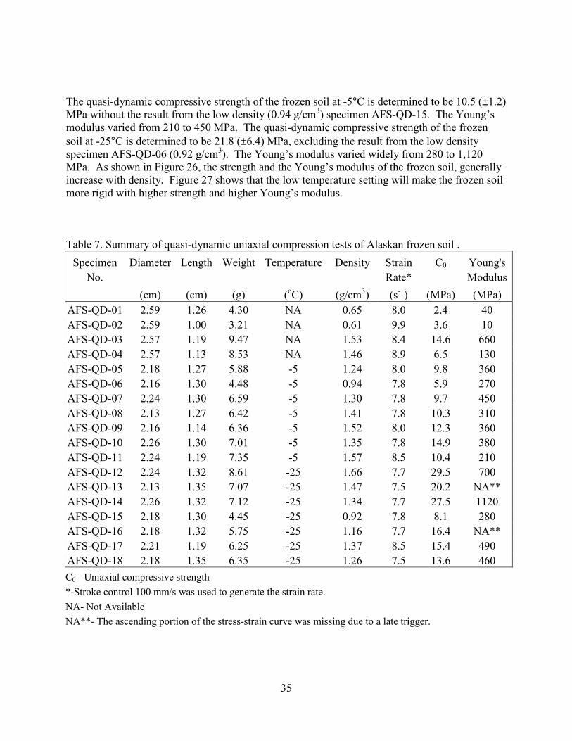
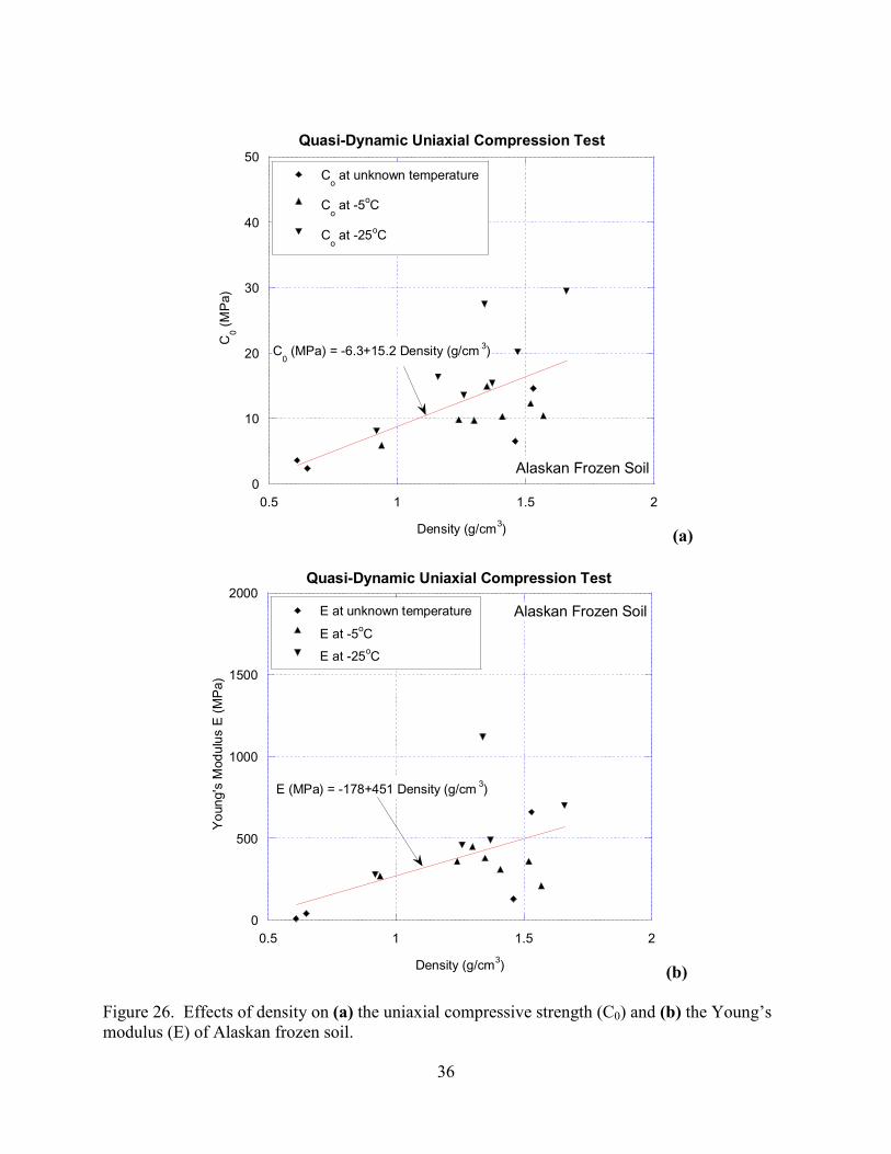
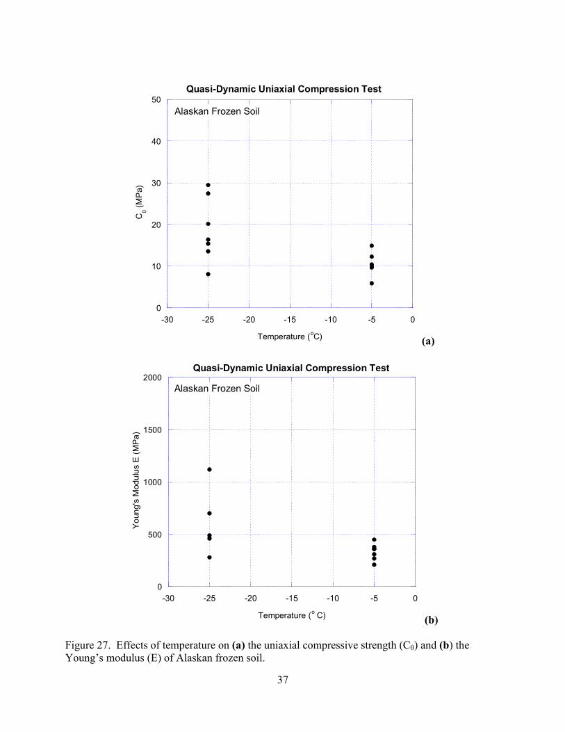
The quasi-dynamic compressive strength of the frozen soil at -5°C is determined to be 10.5 (±1.2)MPa without the result from the low density (0.94 g/cm3) specimen AFS-QD-15. The Young’smodulus varied from 210 to 450 MPa. The quasi-dynamic compressive strength of the frozensoil at -25°C is determined to be 21.8 (±6.4) MPa, excluding the result from the low densityspecimen AFS-QD-06 (0.92 g/cm3). The Young’s modulus varied widely from 280 to 1,120MPa. As shown in Figure 26, the strength and the Young’s modulus of the frozen soil, generallyincrease with density. Figure 27 shows that the low temperature setting will make the frozen soilmore rigid with higher strength and higher Young’s modulus.

Table 7. Summary of quasi-dynamic uniaxial compression tests of Alaskan frozen soil .Specimen Diameter Length Weight Temperature Density Strain C0 Young's

No. Rate* Modulus (cm) (cm) (g) (oC) (g/cm3) (s-1) (MPa) (MPa)

AFS-QD-01 2.59 1.26 4.30 NA 0.65 8.0 2.4 40AFS-QD-02 2.59 1.00 3.21 NA 0.61 9.9 3.6 10AFS-QD-03 2.57 1.19 9.47 NA 1.53 8.4 14.6 660AFS-QD-04 2.57 1.13 8.53 NA 1.46 8.9 6.5 130AFS-QD-05 2.18 1.27 5.88 -5 1.24 8.0 9.8 360AFS-QD-06 2.16 1.30 4.48 -5 0.94 7.8 5.9 270AFS-QD-07 2.24 1.30 6.59 -5 1.30 7.8 9.7 450AFS-QD-08 2.13 1.27 6.42 -5 1.41 7.8 10.3 310AFS-QD-09 2.16 1.14 6.36 -5 1.52 8.0 12.3 360AFS-QD-10 2.26 1.30 7.01 -5 1.35 7.8 14.9 380AFS-QD-11 2.24 1.19 7.35 -5 1.57 8.5 10.4 210AFS-QD-12 2.24 1.32 8.61 -25 1.66 7.7 29.5 700AFS-QD-13 2.13 1.35 7.07 -25 1.47 7.5 20.2 NA**AFS-QD-14 2.26 1.32 7.12 -25 1.34 7.7 27.5 1120AFS-QD-15 2.18 1.30 4.45 -25 0.92 7.8 8.1 280AFS-QD-16 2.18 1.32 5.75 -25 1.16 7.7 16.4 NA**AFS-QD-17 2.21 1.19 6.25 -25 1.37 8.5 15.4 490AFS-QD-18 2.18 1.35 6.35 -25 1.26 7.5 13.6 460C0 - Uniaxial compressive strength*-Stroke control 100 mm/s was used to generate the strain rate.NA- Not AvailableNA**- The ascending portion of the stress-strain curve was missing due to a late trigger.

36

0

10

20

30

40

50

0.5 1 1.5 2

Co at unknown temperature

Co at -5oC

Co at -25oC

C0 (M

Pa)

Density (g/cm3)

Alaskan Frozen Soil

C0 (MPa) = -6.3+15.2 Density (g/cm 3)


(a)

0

500

1000

1500

2000

0.5 1 1.5 2

E at unknown temperature

E at -5oC

E at -25oC

Youn

g's

Mod

ulus

E (M

Pa)

Density (g/cm3)

E (MPa) = -178+451 Density (g/cm 3)


Alaskan Frozen Soil

(b)

Figure 26. Effects of density on (a) the uniaxial compressive strength (C0) and (b) the Young’smodulus (E) of Alaskan frozen soil.

37

0

10

20

30

40

50

-30 -25 -20 -15 -10 -5 0

C0 (M

Pa)

Temperature (oC)

Alaskan Frozen Soil


(a)

0

500

1000

1500

2000

-30 -25 -20 -15 -10 -5 0

Youn

g's

Mod

ulus

E (M

Pa)

Temperature (o C)


Alaskan Frozen Soil

(b)

Figure 27. Effects of temperature on (a) the uniaxial compressive strength (C0) and (b) theYoung’s modulus (E) of Alaskan frozen soil.

38

4.6 Split Hopkinson pressure bar (SHPB) tests

Experimental set-up

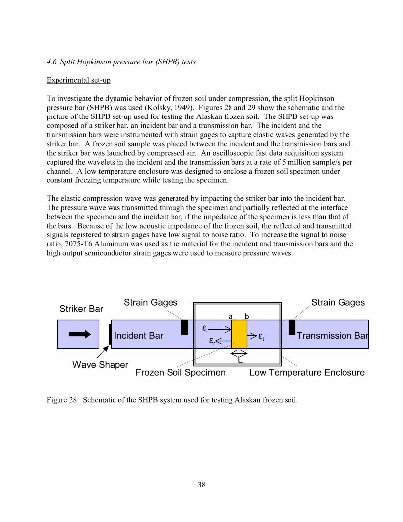
To investigate the dynamic behavior of frozen soil under compression, the split Hopkinsonpressure bar (SHPB) was used (Kolsky, 1949). Figures 28 and 29 show the schematic and thepicture of the SHPB set-up used for testing the Alaskan frozen soil. The SHPB set-up wascomposed of a striker bar, an incident bar and a transmission bar. The incident and thetransmission bars were instrumented with strain gages to capture elastic waves generated by thestriker bar. A frozen soil sample was placed between the incident and the transmission bars andthe striker bar was launched by compressed air. An oscilloscopic fast data acquisition systemcaptured the wavelets in the incident and the transmission bars at a rate of 5 million sample/s perchannel. A low temperature enclosure was designed to enclose a frozen soil specimen underconstant freezing temperature while testing the specimen.

The elastic compression wave was generated by impacting the striker bar into the incident bar.The pressure wave was transmitted through the specimen and partially reflected at the interfacebetween the specimen and the incident bar, if the impedance of the specimen is less than that ofthe bars. Because of the low acoustic impedance of the frozen soil, the reflected and transmittedsignals registered to strain gages have low signal to noise ratio. To increase the signal to noiseratio, 7075-T6 Aluminum was used as the material for the incident and transmission bars and thehigh output semiconductor strain gages were used to measure pressure waves.

Striker Bar

Frozen Soil Specimen

Strain Gages

Wave ShaperLow Temperature Enclosure

a b

L

εiεr

εt Transmission BarIncident Bar

Strain Gages

Figure 28. Schematic of the SHPB system used for testing Alaskan frozen soil.

39

Figure 29. The SHPB testing system used for testing Alaskan frozen soil.

40

Theory of the SHPB testing

When the striker bar impacts the incident bar, an elastic wave is generated and travels through theincident bar. When the elastic wave reached the interface between the incident bar and thespecimen, a fraction of the wave is reflected back into the incident bar due to the impedancemismatch between the sample and the bar. The remainder of the wave travels through thespecimen and reaches the interface between the specimen and the transmission bar. Based on onedimensional theory of elastic wave propagation in a bar and the continuity of displacement andstress equilibrium at the interface, the following equations can be derived to describe stress, strainand strain rate in the specimen (Kolsky, 1949; Lindholm, 1964):

)( ris

a A

AE εεσ +=

)( ts

b A

AE εσ =

rL

C εε 02−=�

tdL

C t

r�=0

02 εε

where σa is the stress in the interface between the sample and the incident bar; σb is the stress inthe interface between the sample and the transmission bar; E is the modulus of the transmissionbar (72 GPa for 7075-T6 Aluminum); A is the cross-sectional area of the transmission bar; As isthe cross-sectional area of the specimen; iε , rε , and tε are the incident, reflected, and transmittedstrains, respectively (see Figure 28); ε� is the strain rate in the specimen; C0 is the longitudinalwave velocity in the incident bar; L is the initial length of the specimen; and t is time.

If the material is very weak, it does not have the stiffness to transmit the high-amplitude loadingon the incident-bar interface through the specimen length effectively. As a result, the portion ofthe specimen near the interface close to the incident bar, gets compacted and pushed quicklytowards the transmitter interface. This compacted section of the specimen experiences large axialacceleration. The stress on the incident-bar interface needs to overcome the inertia induced bythis large acceleration. On the other hand, the transmission bar interface does not "feel" thisacceleration, due to the low strength and low wave speed in the unpacked portion of thespecimen. Therefore, the difference between the two stresses σa and σb will be large for weakmaterials. To achieve an equilibrated stress state and homogeneous deformation throughout the specimen,the load at the incident-bar interface should rise gradually through pulse shaping. Detaileddiscussion on stress equilibrium and homogeneous deformation by pulse shaping can be found inFrew et. al.(2002).

41

Figure 30. Felt metal disk, approximately 1 cm in diameter and 0.2 cm in thickness, used as apulse shaper.

-0.001

-0.0005

0

0.0005

0.001

0 0.0001 0.0002 0.0003 0.0004 0.0005 0.0006

AFS-HB-11

Stra

in (∆

l/l)

Time (s)

Temperature=-5oC

εi - Incident wave

εr - Reflected wave

εt - Transmitted wave

Split Hopkinson Pressure Bar Test

Figure 31. Typical strain-time record obtained during SHPB testing of an Alaskan frozen soilspecimen.

42

0

5

10

15

20

25

0

200

400

600

800

1000

0 5 10-5 0.0001 0.00015 0.0002

AFS-HB-11

Stre

ss (M

Pa)

Strain Rate (s

-1)

Time (s)

Stress

Strain Rate

Temperature=-5oC


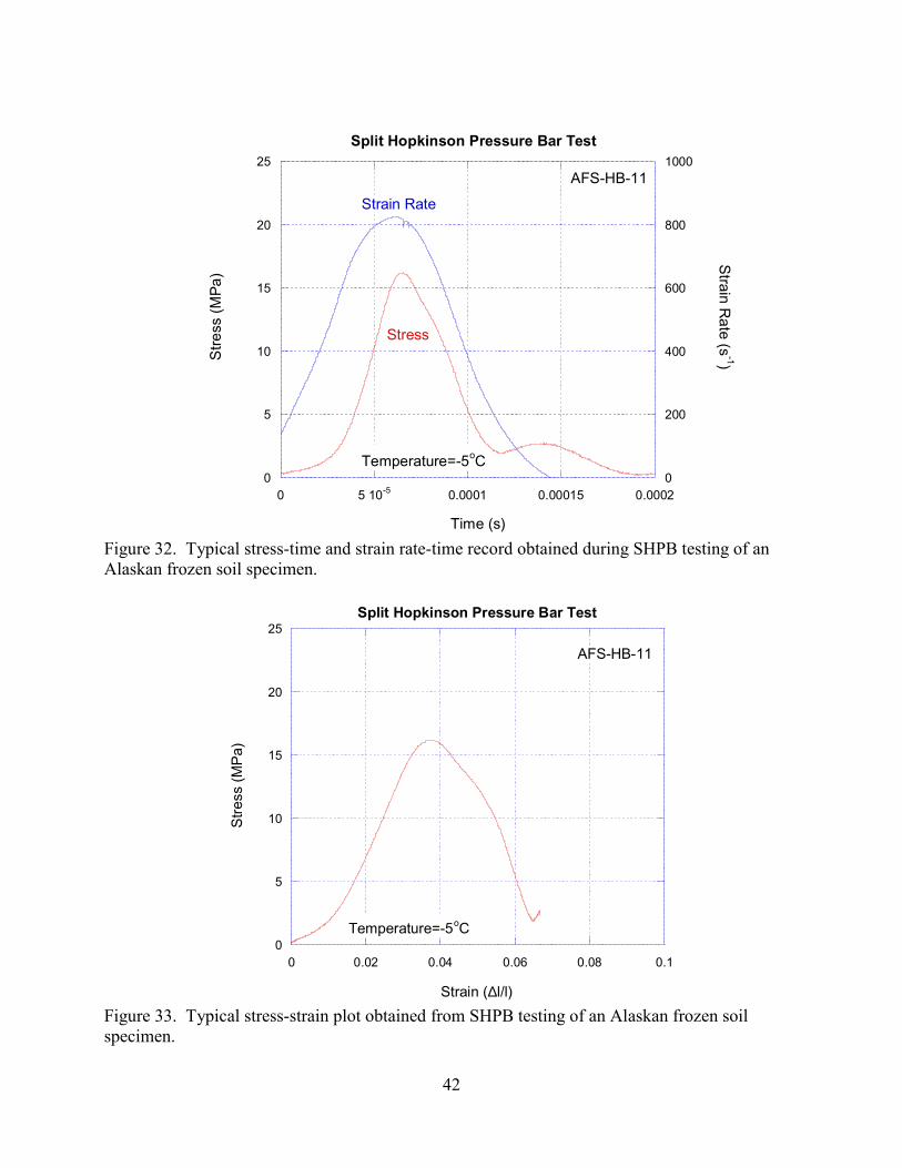
Figure 32. Typical stress-time and strain rate-time record obtained during SHPB testing of anAlaskan frozen soil specimen.

0

5

10

15

20

25

0 0.02 0.04 0.06 0.08 0.1

AFS-HB-11

Stre

ss (M

Pa)

Strain (∆l/l)

Temperature=-5oC


Figure 33. Typical stress-strain plot obtained from SHPB testing of an Alaskan frozen soilspecimen.

43

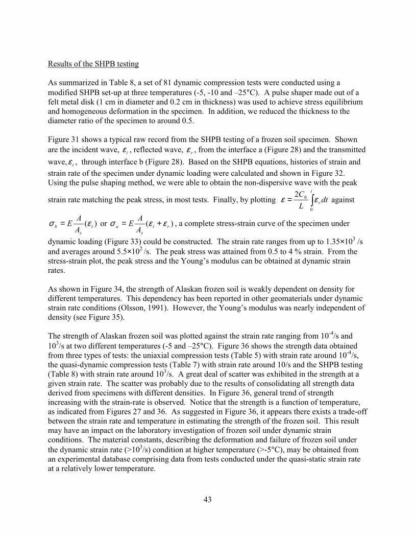
Results of the SHPB testing

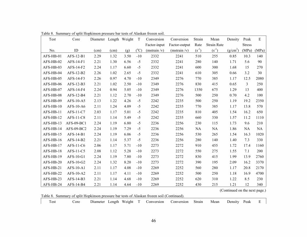
As summarized in Table 8, a set of 81 dynamic compression tests were conducted using amodified SHPB set-up at three temperatures (-5, -10 and –25°C). A pulse shaper made out of afelt metal disk (1 cm in diameter and 0.2 cm in thickness) was used to achieve stress equilibriumand homogeneous deformation in the specimen. In addition, we reduced the thickness to thediameter ratio of the specimen to around 0.5.

Figure 31 shows a typical raw record from the SHPB testing of a frozen soil specimen. Shownare the incident wave, iε , reflected wave, rε , from the interface a (Figure 28) and the transmittedwave, tε , through interface b (Figure 28). Based on the SHPB equations, histories of strain andstrain rate of the specimen under dynamic loading were calculated and shown in Figure 32.Using the pulse shaping method, we were able to obtain the non-dispersive wave with the peak

strain rate matching the peak stress, in most tests. Finally, by plotting tdL

C t

r�=0

02 εε against

)( ts

b A

AE εσ = or )( ri

sa A

AE εεσ += , a complete stress-strain curve of the specimen under

dynamic loading (Figure 33) could be constructed. The strain rate ranges from up to 1.35×103 /sand averages around 5.5×102 /s. The peak stress was attained from 0.5 to 4 % strain. From thestress-strain plot, the peak stress and the Young’s modulus can be obtained at dynamic strainrates.

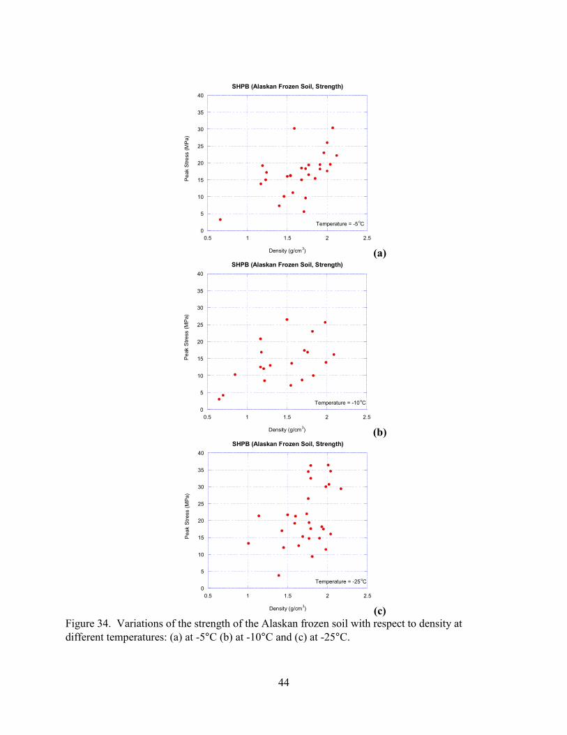
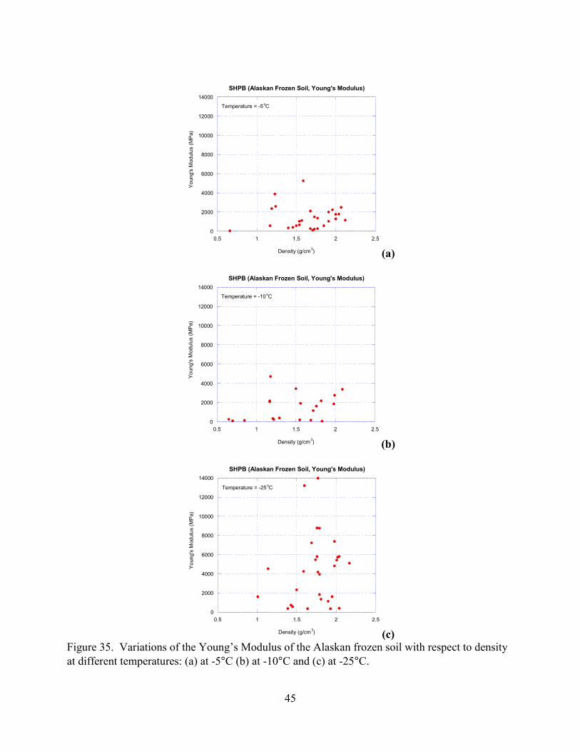
As shown in Figure 34, the strength of Alaskan frozen soil is weakly dependent on density fordifferent temperatures. This dependency has been reported in other geomaterials under dynamicstrain rate conditions (Olsson, 1991). However, the Young’s modulus was nearly independent ofdensity (see Figure 35).

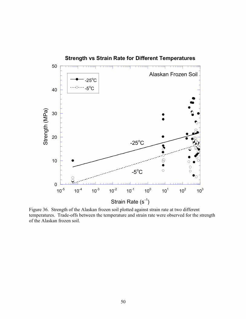
The strength of Alaskan frozen soil was plotted against the strain rate ranging from 10-4/s and103/s at two different temperatures (-5 and –25°C). Figure 36 shows the strength data obtainedfrom three types of tests: the uniaxial compression tests (Table 5) with strain rate around 10-4/s,the quasi-dynamic compression tests (Table 7) with strain rate around 10/s and the SHPB testing(Table 8) with strain rate around 103/s. A great deal of scatter was exhibited in the strength at agiven strain rate. The scatter was probably due to the results of consolidating all strength dataderived from specimens with different densities. In Figure 36, general trend of strengthincreasing with the strain-rate is observed. Notice that the strength is a function of temperature,as indicated from Figures 27 and 36. As suggested in Figure 36, it appears there exists a trade-offbetween the strain rate and temperature in estimating the strength of the frozen soil. This resultmay have an impact on the laboratory investigation of frozen soil under dynamic strainconditions. The material constants, describing the deformation and failure of frozen soil underthe dynamic strain rate (>103/s) condition at higher temperature (>-5°C), may be obtained froman experimental database comprising data from tests conducted under the quasi-static strain rateat a relatively lower temperature.

44

0

5

10

15

20

25

30

35

40

0.5 1 1.5 2 2.5

SHPB (Alaskan Frozen Soil, Strength)

Peak

Stre

ss (M

Pa)

Density (g/cm3)

Temperature = -5oC

(a)

0

5

10

15

20

25

30

35

40

0.5 1 1.5 2 2.5


Peak

Stre

ss (M

Pa)

Density (g/cm3)

Temperature = -10oC

(b)

0

5

10

15

20

25

30

35

40

0.5 1 1.5 2 2.5


Pea

k St

ress

(MPa

)

Density (g/cm3)

Temperature = -25oC

(c)Figure 34. Variations of the strength of the Alaskan frozen soil with respect to density atdifferent temperatures: (a) at -5°C (b) at -10°C and (c) at -25°C.

45

0

2000

4000

6000

8000

10000

12000

14000

0.5 1 1.5 2 2.5

SHPB (Alaskan Frozen Soil, Young's Modulus)

Youn

g's

Mod

ulus

(MP

a)

Density (g/cm3)

Temperature = -5oC

(a)

0

2000

4000

6000

8000

10000

12000

14000

0.5 1 1.5 2 2.5


Youn

g's

Mod

ulus

(MPa

)

Density (g/cm3)

Temperature = -10oC

(b)

0

2000

4000

6000

8000

10000

12000

14000

0.5 1 1.5 2 2.5


Youn

g's

Mod

ulus

(MP

a)

Density (g/cm3)

Temperature = -25oC

(c)Figure 35. Variations of the Young’s Modulus of the Alaskan frozen soil with respect to densityat different temperatures: (a) at -5°C (b) at -10°C and (c) at -25°C.

46

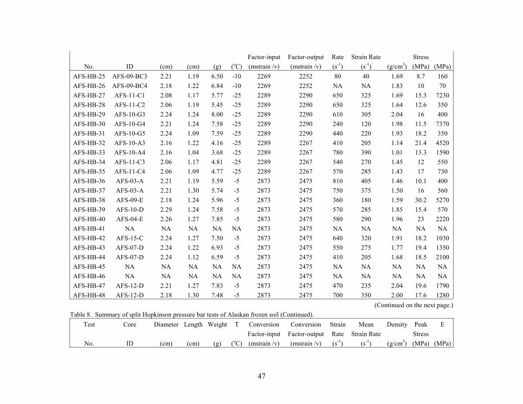
Table 8. Summary of split Hopkinson pressure bar tests of Alaskan frozen soil.Test Core Diameter Length Weight T Conversion Conversion Strain Mean Density Peak E

Factor-input Factor-output Rate Strain Rate Stress No. ID (cm) (cm) (g) (oC) (mstrain /v) (mstrain /v) (s-1) (s-1) (g/cm3) (MPa) (MPa)

AFS-HB-01 AFS-12-B1 2.29 1.32 3.50 -10 2332 2241 510 255 0.85 10.3 140AFS-HB-02 AFS-14-F1 2.21 1.30 6.56 -5 2332 2241 280 140 1.71 5.6 90AFS-HB-03 AFS-14-F2 2.24 1.17 6.60 -5 2332 2241 600 300 1.68 15 270AFS-HB-04 AFS-12-B2 2.26 1.02 2.65 -5 2332 2241 610 305 0.66 3.2 30AFS-HB-05 AFS-14-F3 2.26 0.97 4.70 -10 2349 2276 770 385 1.17 12.5 2080AFS-HB-06 AFS-12-B3 2.21 1.02 2.50 -10 2349 2276 830 415 0.65 3 250AFS-HB-07 AFS-14-F4 2.24 0.94 5.05 -10 2349 2276 1350 675 1.29 13 400AFS-HB-08 AFS-12-B4 2.21 1.12 2.70 -10 2349 2276 500 250 0.70 4.2 100AFS-HB-09 AFS-10-A5 2.13 1.22 4.26 -5 2242 2235 500 250 1.19 19.2 2350AFS-HB-10 AFS-10-A6 2.11 1.24 4.09 -5 2242 2235 770 385 1.17 13.8 570AFS-HB-11 AFS-11-C7 2.03 1.17 5.01 -5 2242 2235 810 405 1.54 16.2 650AFS-HB-12 AFS-11-C8 2.11 1.14 5.49 -5 2242 2235 660 330 1.57 11.2 1110AFS-HB-13 AFS-09-BC1 2.24 1.19 6.80 -5 2236 2256 230 115 1.73 9.6 210AFS-HB-14 AFS-09-BC2 2.24 1.19 7.29 -5 2236 2256 NA NA 1.86 NA NAAFS-HB-15 AFS-14-B1 2.24 1.19 6.06 -5 2236 2256 530 265 1.54 16.3 1020AFS-HB-16 AFS-14-B2 2.21 1.14 5.37 -5 2236 2256 280 140 1.40 7.3 330AFS-HB-17 AFS-11-C6 2.06 1.17 5.71 -10 2273 2272 910 455 1.72 17.4 1160AFS-HB-18 AFS-11-C5 2.08 1.12 5.28 -10 2273 2272 550 275 1.55 7.1 200AFS-HB-19 AFS-10-G1 2.24 1.19 7.80 -10 2273 2272 830 415 1.99 13.9 2760AFS-HB-20 AFS-10-G2 2.24 1.32 8.20 -10 2273 2272 390 195 2.09 16.2 3370AFS-HB-21 AFS-10-A1 2.11 1.17 4.08 -10 2269 2252 560 280 1.17 20.8 2170AFS-HB-22 AFS-10-A2 2.11 1.17 4.11 -10 2269 2252 500 250 1.18 16.9 4700AFS-HB-23 AFS-14-B3 2.21 1.14 4.68 -10 2269 2252 620 310 1.22 8.5 230AFS-HB-24 AFS-14-B4 2.21 1.14 4.64 -10 2269 2252 430 215 1.21 12 340

(Continued on the next page.)Table 8. Summary of split Hopkinson pressure bar tests of Alaskan frozen soil (Continued).

Test Core Diameter Length Weight T Conversion Conversion Strain Mean Density Peak E

47

Factor-input Factor-output Rate Strain Rate Stress No. ID (cm) (cm) (g) (oC) (mstrain /v) (mstrain /v) (s-1) (s-1) (g/cm3) (MPa) (MPa)

AFS-HB-25 AFS-09-BC3 2.21 1.19 6.50 -10 2269 2252 80 40 1.69 8.7 160AFS-HB-26 AFS-09-BC4 2.18 1.22 6.84 -10 2269 2252 NA NA 1.83 10 70AFS-HB-27 AFS-11-C1 2.08 1.17 5.77 -25 2289 2290 650 325 1.69 15.3 7230AFS-HB-28 AFS-11-C2 2.06 1.19 5.45 -25 2289 2290 650 325 1.64 12.6 350AFS-HB-29 AFS-10-G3 2.24 1.24 8.00 -25 2289 2290 610 305 2.04 16 400AFS-HB-30 AFS-10-G4 2.21 1.24 7.58 -25 2289 2290 240 120 1.98 11.5 7370AFS-HB-31 AFS-10-G5 2.24 1.09 7.59 -25 2289 2290 440 220 1.93 18.2 350AFS-HB-32 AFS-10-A3 2.16 1.22 4.16 -25 2289 2267 410 205 1.14 21.4 4520AFS-HB-33 AFS-10-A4 2.16 1.04 3.68 -25 2289 2267 780 390 1.01 13.3 1590AFS-HB-34 AFS-11-C3 2.06 1.17 4.81 -25 2289 2267 540 270 1.45 12 550AFS-HB-35 AFS-11-C4 2.06 1.09 4.77 -25 2289 2267 570 285 1.43 17 730AFS-HB-36 AFS-03-A 2.21 1.19 5.59 -5 2873 2475 810 405 1.46 10.1 400AFS-HB-37 AFS-03-A 2.21 1.30 5.74 -5 2873 2475 750 375 1.50 16 560AFS-HB-38 AFS-09-E 2.18 1.24 5.96 -5 2873 2475 360 180 1.59 30.2 5270AFS-HB-39 AFS-10-D 2.29 1.24 7.58 -5 2873 2475 570 285 1.85 15.4 570AFS-HB-40 AFS-04-E 2.26 1.27 7.85 -5 2873 2475 580 290 1.96 23 2220AFS-HB-41 NA NA NA NA NA 2873 2475 NA NA NA NA NAAFS-HB-42 AFS-15-C 2.24 1.27 7.50 -5 2873 2475 640 320 1.91 18.2 1030AFS-HB-43 AFS-07-D 2.24 1.22 6.93 -5 2873 2475 550 275 1.77 19.4 1350AFS-HB-44 AFS-07-D 2.24 1.12 6.59 -5 2873 2475 410 205 1.68 18.5 2100AFS-HB-45 NA NA NA NA NA 2873 2475 NA NA NA NA NAAFS-HB-46 NA NA NA NA NA 2873 2475 NA NA NA NA NAAFS-HB-47 AFS-12-D 2.21 1.27 7.83 -5 2873 2475 470 235 2.04 19.6 1790AFS-HB-48 AFS-12-D 2.18 1.30 7.48 -5 2873 2475 700 350 2.00 17.6 1280


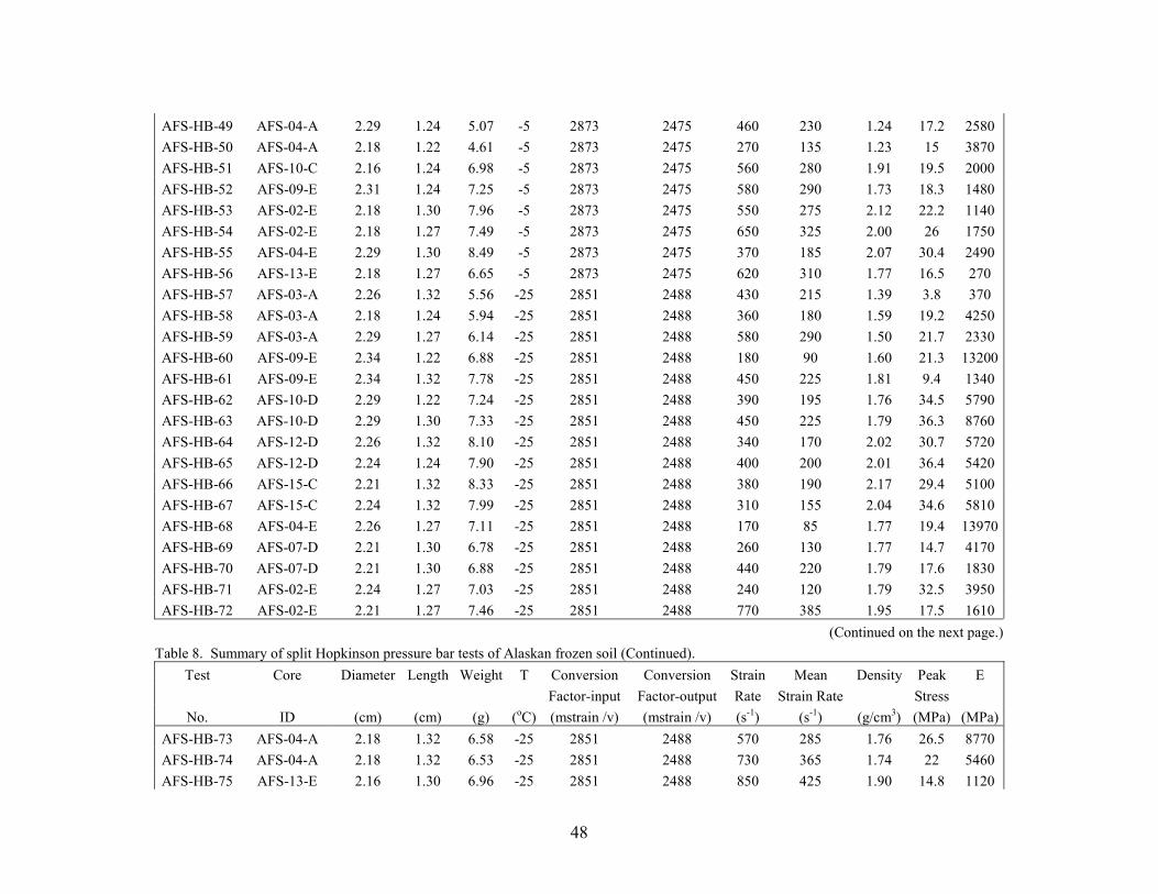
Test Core Diameter Length Weight T Conversion Conversion Strain Mean Density Peak E Factor-input Factor-output Rate Strain Rate Stress

No. ID (cm) (cm) (g) (oC) (mstrain /v) (mstrain /v) (s-1) (s-1) (g/cm3) (MPa) (MPa)

48

AFS-HB-49 AFS-04-A 2.29 1.24 5.07 -5 2873 2475 460 230 1.24 17.2 2580AFS-HB-50 AFS-04-A 2.18 1.22 4.61 -5 2873 2475 270 135 1.23 15 3870AFS-HB-51 AFS-10-C 2.16 1.24 6.98 -5 2873 2475 560 280 1.91 19.5 2000AFS-HB-52 AFS-09-E 2.31 1.24 7.25 -5 2873 2475 580 290 1.73 18.3 1480AFS-HB-53 AFS-02-E 2.18 1.30 7.96 -5 2873 2475 550 275 2.12 22.2 1140AFS-HB-54 AFS-02-E 2.18 1.27 7.49 -5 2873 2475 650 325 2.00 26 1750AFS-HB-55 AFS-04-E 2.29 1.30 8.49 -5 2873 2475 370 185 2.07 30.4 2490AFS-HB-56 AFS-13-E 2.18 1.27 6.65 -5 2873 2475 620 310 1.77 16.5 270AFS-HB-57 AFS-03-A 2.26 1.32 5.56 -25 2851 2488 430 215 1.39 3.8 370AFS-HB-58 AFS-03-A 2.18 1.24 5.94 -25 2851 2488 360 180 1.59 19.2 4250AFS-HB-59 AFS-03-A 2.29 1.27 6.14 -25 2851 2488 580 290 1.50 21.7 2330AFS-HB-60 AFS-09-E 2.34 1.22 6.88 -25 2851 2488 180 90 1.60 21.3 13200AFS-HB-61 AFS-09-E 2.34 1.32 7.78 -25 2851 2488 450 225 1.81 9.4 1340AFS-HB-62 AFS-10-D 2.29 1.22 7.24 -25 2851 2488 390 195 1.76 34.5 5790AFS-HB-63 AFS-10-D 2.29 1.30 7.33 -25 2851 2488 450 225 1.79 36.3 8760AFS-HB-64 AFS-12-D 2.26 1.32 8.10 -25 2851 2488 340 170 2.02 30.7 5720AFS-HB-65 AFS-12-D 2.24 1.24 7.90 -25 2851 2488 400 200 2.01 36.4 5420AFS-HB-66 AFS-15-C 2.21 1.32 8.33 -25 2851 2488 380 190 2.17 29.4 5100AFS-HB-67 AFS-15-C 2.24 1.32 7.99 -25 2851 2488 310 155 2.04 34.6 5810AFS-HB-68 AFS-04-E 2.26 1.27 7.11 -25 2851 2488 170 85 1.77 19.4 13970AFS-HB-69 AFS-07-D 2.21 1.30 6.78 -25 2851 2488 260 130 1.77 14.7 4170AFS-HB-70 AFS-07-D 2.21 1.30 6.88 -25 2851 2488 440 220 1.79 17.6 1830AFS-HB-71 AFS-02-E 2.24 1.27 7.03 -25 2851 2488 240 120 1.79 32.5 3950AFS-HB-72 AFS-02-E 2.21 1.27 7.46 -25 2851 2488 770 385 1.95 17.5 1610


Test Core Diameter Length Weight T Conversion Conversion Strain Mean Density Peak E Factor-input Factor-output Rate Strain Rate Stress

No. ID (cm) (cm) (g) (oC) (mstrain /v) (mstrain /v) (s-1) (s-1) (g/cm3) (MPa) (MPa)AFS-HB-73 AFS-04-A 2.18 1.32 6.58 -25 2851 2488 570 285 1.76 26.5 8770AFS-HB-74 AFS-04-A 2.18 1.32 6.53 -25 2851 2488 730 365 1.74 22 5460AFS-HB-75 AFS-13-E 2.16 1.30 6.96 -25 2851 2488 850 425 1.90 14.8 1120

49

AFS-HB-76 AFS-10-C 2.18 1.27 7.43 -25 2851 2488 800 400 1.98 30 4820AFS-HB-77 AFS-03-A 2.18 1.24 5.85 -10 2873 2475 850 425 1.56 13.6 1910AFS-HB-78 AFS-03-A 2.21 1.27 5.75 -10 2873 2475 720 360 1.50 26.5 3440AFS-HB-79 AFS-12-D 2.26 1.27 7.93 -10 2873 2475 800 400 1.98 25.7 1860AFS-HB-80 AFS-02-E 2.24 1.19 7.16 -10 2873 2475 640 320 1.82 23 2190AFS-HB-81 AFS-07-D 2.18 1.17 6.60 -10 2873 2475 470 235 1.76 16.9 1630

SHPB input and output bar material - Aluminum 7075-T6 extrusionAl. Bar wave velocity = 6.3 km / sAl. Bar Young's modulus = 72 GPaAl. Bar diameter = 2.54 cmE=Young's Modulus; T=TemperatureMean strain rate=0.5*strain rate

50

0

10

20

30

40

50

10-5 10-4 10-3 10-2 10-1 100 101 102 103

Strength vs Strain Rate for Different Temperatures

-25oC

-5oC

Stre

ngth

(MPa

)

Strain Rate (s-1)

Alaskan Frozen Soil

-25oC

-5oC

Figure 36. Strength of the Alaskan frozen soil plotted against strain rate at two differenttemperatures. Trade-offs between the temperature and strain rate were observed for the strengthof the Alaskan frozen soil.

51

5. Constitutive Modeling

Laboratory material testing showed that Alaskan frozen soil exhibits pressure and temperaturedependence, rate sensitivity, anisotropy, brittle and ductile behavior, volumetric compaction, anddilation. A constitutive equation capable of modeling such a complex material is the rate-sensitive, anisotropic version of a plasticity model being developed by Fossum and Fredrich(2000). This model includes high strain-rate sensitivity and anisotropy in both the elastic andplastic regimes. The model is defined through a continuous yield and loading surface for unifieddilation and compaction phenomena. Included are a pore collapse mechanism, shear failuremechanism, and a cleavage failure mechanism.

For frozen soil, it is sufficient to limit the anisotropy to transverse isotropy. In the following, itis assumed that anisotropy occurs in the 11 direction as depicted in Figure 37.

2233

11

Figure 37. The constitutive model is developed for a transversely isotropic material

In general, the tensor form of Hooke’s law is written in terms of a fourth-order coefficientmatrix, Cijkl, as

klijklij C εσ =

If the stresses ijσ and elastic strains eklε are ordered according to ( iσ , e

iε , i = 11, 22, 33, 12, 13,

23), then Hooke’s Law can be written in terms of a second-order coefficient matrix, which fortransversely isotropic materials is given by

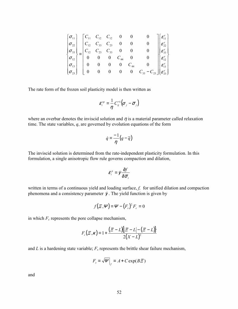
52

The rate form of the frozen soil plasticity model is then written as

( )jjijvpi C σσ

ηε −= −11�

where an overbar denotes the inviscid solution and η is a material parameter called relaxationtime. The state variables, q, are governed by evolution equations of the form

( )qqq −−=η

1�

The inviscid solution is determined from the rate-independent plasticity formulation. In thisformulation, a single anisotropic flow rule governs compaction and dilation,

i

pi

f

σγε

∂∂= ��

written in terms of a continuous yield and loading surface, f, for unified dilation and compactionphenomena and a consistency parameter γ� . The yield function is given by

( ) ( ) 0, 2 =−= cs FFf ΨΨΞ

in which Fc represents the pore collapse mechanism,

( ) ( ) ( ){ }( )22

1,LX

LLLFc −

−−−−+=

ΞΞΞκΞ

and L is a hardening state variable; Fs represents the brittle shear failure mechanism,

)exp( ΞΨ BCAFf

s +==

and

��

�

��

�

�

��

�

��

�

�

��

��

�

−

=

��

�

��

�

�

��

�

��

�

�

e

e

e

e

e

e

CC

C

C

CCC

CCC

CCC

23

13

12

33

22

11

2333

44

44

332312

233312

121211

23

13

12

33

22

11

000000000000000000000000

εεεεεε

σσσσσσ

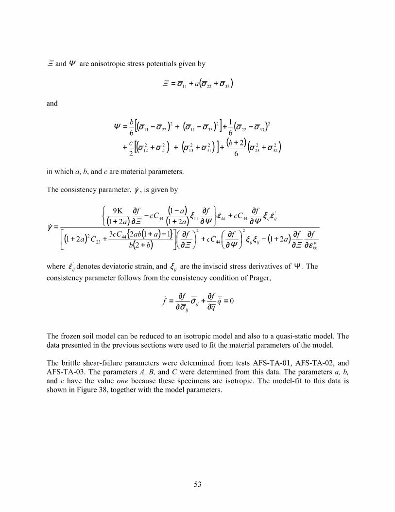
53

ΨΞ and are anisotropic stress potentials given by

( )332211 σσσΞ ++= a

and

( ) ( )[ ] ( )

( ) ( )[ ] ( ) ( )232

223

231

213

221

212

23322

23311

22211

62

2

61

6

σσσσσσ

σσσσσσΨ

+++++++

−+−+−=

bc

b

in which a, b, and c are material parameters.

The consistency parameter, γ� , is given by

( )( )( )

( ) ( ){ }( ) ( )

pkk

ijij

ijijkk

ffa

fcC

f

bb

aabcCCa

fcC

f

a

acC

f

a

εΞξξ

ΨΞ

εξΨ

εΨ

ξΞ

γ

∂∂

∂∂+−�

�

��

�

∂∂+�

�

��

�

∂∂

��

�

�

+−+++

∂∂+

��

��

∂∂

+−−

∂∂

+=

212

112321

211

21K9

2

44

244

232

'441144 ��

�

where 'ijε� denotes deviatoric strain, and ijξ are the inviscid stress derivatives of Ψ . The

consistency parameter follows from the consistency condition of Prager,

0=∂∂+

∂∂= q

q

fff ij

ij

�� σσ

The frozen soil model can be reduced to an isotropic model and also to a quasi-static model. Thedata presented in the previous sections were used to fit the material parameters of the model.

The brittle shear-failure parameters were determined from tests AFS-TA-01, AFS-TA-02, andAFS-TA-03. The parameters A, B, and C were determined from this data. The parameters a, b,and c have the value one because these specimens are isotropic. The model-fit to this data isshown in Figure 38, together with the model parameters.

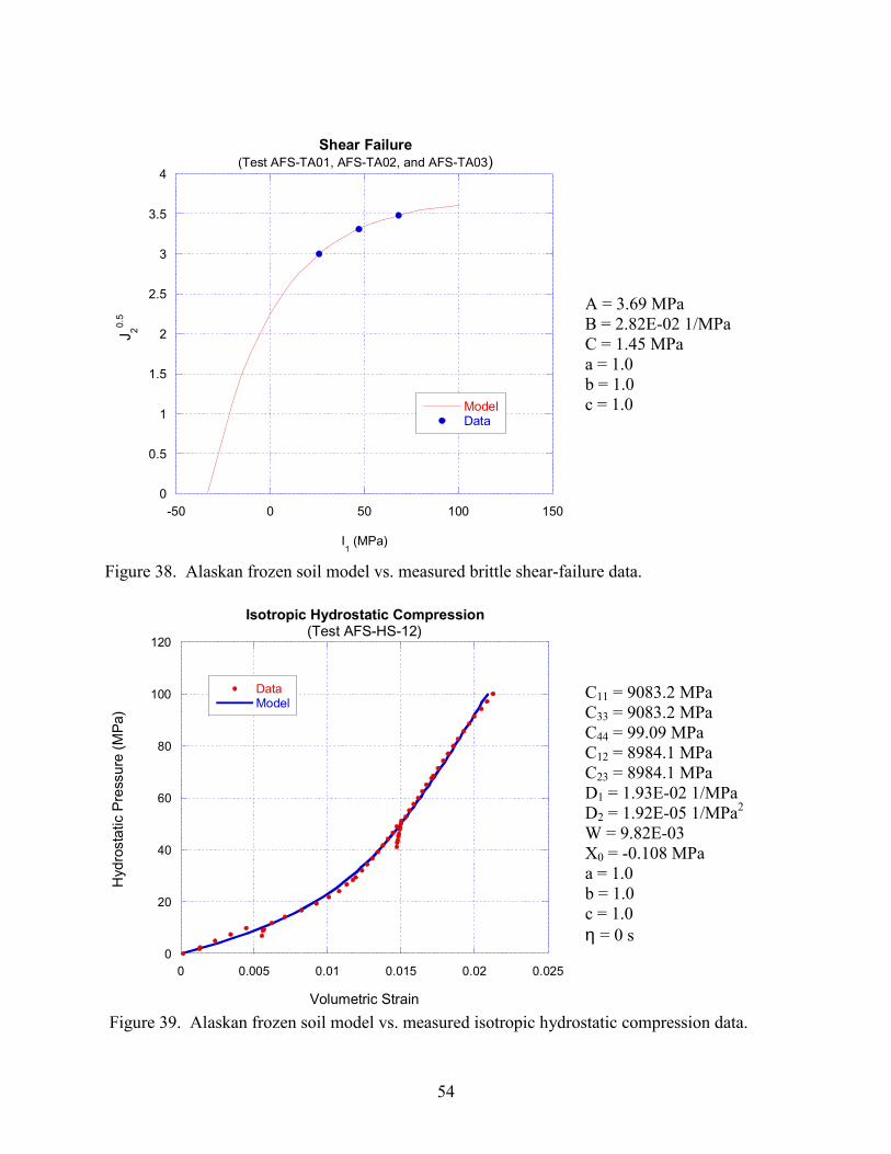
54

0

0.5

1

1.5

2

2.5

3

3.5

4

-50 0 50 100 150

Shear Failure(Test AFS-TA01, AFS-TA02, and AFS-TA03)

ModelData

J 20.5

I1 (MPa)

A = 3.69 MPaB = 2.82E-02 1/MPaC = 1.45 MPaa = 1.0b = 1.0c = 1.0

Figure 38. Alaskan frozen soil model vs. measured brittle shear-failure data.

0

20

40

60

80

100

120

0 0.005 0.01 0.015 0.02 0.025

Isotropic Hydrostatic Compression(Test AFS-HS-12)

DataModel

Hyd

rost

atic

Pre

ssur

e (M

Pa)

Volumetric Strain

C11 = 9083.2 MPaC33 = 9083.2 MPaC44 = 99.09 MPaC12 = 8984.1 MPaC23 = 8984.1 MPaD1 = 1.93E-02 1/MPaD2 = 1.92E-05 1/MPa2

W = 9.82E-03X0 = -0.108 MPaa = 1.0b = 1.0c = 1.0η = 0 s

Figure 39. Alaskan frozen soil model vs. measured isotropic hydrostatic compression data.

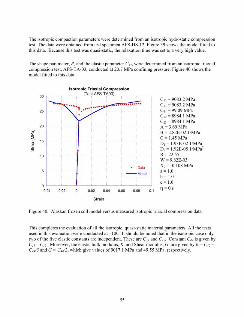
55

The isotropic compaction parameters were determined from an isotropic hydrostatic compressiontest. The data were obtained from test specimen AFS-HS-12. Figure 39 shows the model fitted tothis data. Because this test was quasi-static, the relaxation time was set to a very high value.

The shape parameter, R, and the elastic parameter C44, were determined from an isotropic triaxialcompression test, AFS-TA-03, conducted at 20.7 MPa confining pressure. Figure 40 shows themodel fitted to this data.

0

5

10

15

20

25

30

-0.04 -0.02 0 0.02 0.04 0.06 0.08 0.1

Isotropic Triaxial Compression(Test AFS-TA03)

Data

Model

Stre

a (M

Pa)

Strain

C11 = 9083.2 MPaC33 = 9083.2 MPaC44 = 99.09 MPaC12 = 8984.1 MPaC23 = 8984.1 MPaA = 3.69 MPaB = 2.82E-02 1/MPaC = 1.45 MPaD1 = 1.93E-02 1/MPaD2 = 1.92E-05 1/MPa2

R = 22.55W = 9.82E-03X0 = -0.108 MPaa = 1.0b = 1.0c = 1.0η = 0 s

Figure 40. Alaskan frozen soil model versus measured isotropic triaxial compression data.

This completes the evaluation of all the isotropic, quasi-static material parameters. All the testsused in this evaluation were conducted at –10C. It should be noted that in the isotropic case onlytwo of the five elastic constants are independent. These are C11 and C12. Constant C44 is given byC11 – C12. Moreover, the elastic bulk modulus, K, and Shear modulus, G, are given by K = C12 +C44/3 and G = C44/2, which give values of 9017.1 MPa and 49.55 MPa, respectively.

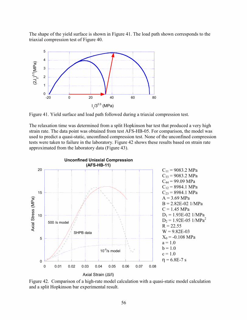
56

The shape of the yield surface is shown in Figure 41. The load path shown corresponds to thetriaxial compression test of Figure 40.

0

1

2

3

4

5

-20 0 20 40 60 80

(2J 2)0.

5 (MPa

)

I1/30.5 (MPa)

Figure 41. Yield surface and load path followed during a triaxial compression test.

The relaxation time was determined from a split Hopkinson bar test that produced a very highstrain rate. The data point was obtained from test AFS-HB-05. For comparison, the model wasused to predict a quasi-static, unconfined compression test. None of the unconfined compressiontests were taken to failure in the laboratory. Figure 42 shows these results based on strain rateapproximated from the laboratory data (Figure 43).

0

5

10

15

20

0 0.01 0.02 0.03 0.04 0.05 0.06 0.07 0.08

Unconfined Uniaxial Compression(AFS-HB-11)

Axia

l Stre

ss (M

Pa)

Axial Strain (∆l/l)

10-5/s model

500 /s model

SHPB data


R = 22.55W = 9.82E-03X0 = -0.108 MPaa = 1.0b = 1.0c = 1.0η = 6.8E-7 s

Figure 42. Comparison of a high-rate model calculation with a quasi-static model calculationand a split Hopkinson bar experimental result.

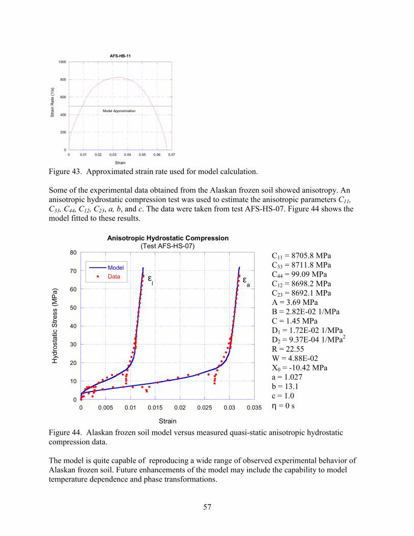
57

0

200

400

600

800

1000

0 0.01 0.02 0.03 0.04 0.05 0.06 0.07

AFS-HB-11St

rain

Rat

e (1

/s)

Strain

Model Approximation

Figure 43. Approximated strain rate used for model calculation.

Some of the experimental data obtained from the Alaskan frozen soil showed anisotropy. Ananisotropic hydrostatic compression test was used to estimate the anisotropic parameters C11,C33, C44, C12, C23, a, b, and c. The data were taken from test AFS-HS-07. Figure 44 shows themodel fitted to these results.

0

10

20

30

40

50

60

70

80

0 0.005 0.01 0.015 0.02 0.025 0.03 0.035

Anisotropic Hydrostatic Compression(Test AFS-HS-07)

ModelData

Hyd

rost

atic

Stre

ss (M

Pa)

Strain

εa

εl


R = 22.55W = 4.88E-02X0 = -10.42 MPaa = 1.027b = 13.1c = 1.0η = 0 s

Figure 44. Alaskan frozen soil model versus measured quasi-static anisotropic hydrostaticcompression data.

The model is quite capable of reproducing a wide range of observed experimental behavior ofAlaskan frozen soil. Future enhancements of the model may include the capability to modeltemperature dependence and phase transformations.

58

6. Conclusions

To obtain a well-determined data set of Alaskan frozen soil, a series of quasi-static, quasi-dynamic and dynamic compression tests was conducted using unique high-pressure, low-temperature apparatus and the split Hopkinson pressure bar (SHPB). The results from laboratoryconstitutive experiments can be summarized as follows:

• Alaskan Frozen Soil is a temperature dependent, anisotropic material. The density of thefrozen soil depends on the depth of the soil measured from the surface. The near-surfacelayer (< 1 m) consists of a low density organic material, layered subparallel to the surface.

• The material properties of Alaskan Frozen Soil are largely dependent on the density of thesoil.

• The material properties database for Alaskan Frozen Soil has been established based on fivetypes of laboratory tests: Brazilian indirect tension test, hydrostatic compression test,uniaxial compression test conducted at the strain rate of around 10-4/s, quasi-dynamiccompression test conducted at the strain rate of around 10/s, and the SHPB test conducted atthe strain rate of around 103/s. The results are summarized in Tables 3 through 8.

• The ice trapped in the Alaskan Frozen Soil may have been transformed into water near 100MPa confining pressure at -10ºC. The phase transformation may affect the materialproperties of Alaskan Frozen Soil under the high impact pressure.

• Alaskan frozen soil compacts and then dilates during triaxial testing.

• A trade-off between the strain rate and the temperature exists in estimating the strength of thefrozen soil.

59

References

ASTM D3967, Standard Test Method for Splitting Tensile Strength of Intact Rock CoreSpecimens, American Society for Testing and Materials, 1995.

ASTM D4543, Standard Practice for Preparing Rock Core Specimens and DeterminingDimensional and Shape Tolerances, American Society for Testing and Materials, 1995.

Chamberlain, E., Groves, C. and R. Perham, Mechanical Behaviour of Frozen Earth Materialsunder High Pressure Triaxial Test Condition, Geotechique, 22, No. 3, 469-481, 1972.

Durham, W.B., Heard, H.C. and S.H. Kirby, Experimental Deformation of Polycrystalline H2OIce at High Pressure and Low Temperature: Preliminary Results, JGR, Vol.88, 377-392, 1983.

Fossum, A.F. and J.T. Fredrich, Cap Plasticity Models and Compactive and Pliant Pre-FailureDeformation, Proceedings of the Fourth North American Rock Mechanics Symposium, NARMS2000, Seattle, Washington, 1169-1176, 2000.

Frew D.J., Forrestal, M.J. and W. Chen, Pulse Shaping Techniques for Testing Brittle Materialswith a Split Hopkinson Pressure Bar, Experimental Mechanics, 2002.

Gratz, E. T. and E. M. Schulson, The Deformation of Cubes of Frozen Soil Loaded underTriaxial Compression, Final Report, Project No. AN-2014, 94 p., Thayer School of Engineering,Dartmouth College, Hanover, New Hampshire, 1996.

Hardy, R., Event Triggered Data Acquisition in the Rock Mechanics Laboratory, Sandia ReportSAND93-0256, UC-403, Sandia National Laboratories, Albuquerque NM., 1993.

Jaeger, J.C. and N.G.W. Cook, Fundamentals of Rock Mechanics, 102-106, Methuen, London,England, 1969.

Kolsky, H., An Investigation of the Mechanical Properties of Materials at Very High Rates ofStrain, Proc. Roy. Phys. Soc., B62, 676-700, 1949.

Lindholm, U.S., Some Experiments with the Split Hopkinson Pressure Bar, J. Mech. Phys.Solids, Vol.12, 317-335, Pergamon, 1964.

Olsson, W.A., The Compressive Strength of Tuff as a Function of Strain Rate from 10-6 to103/sec, Int. J. Rock Mech. Min. Sci. & Geomech. Abstr. Vol. 28, No.1, 115-118, 1991.

Ueda, H., Sellmann, P. and G. Abele, USA CRREL Snow and Ice Testing Equipment, US ArmyCorps of Engineers, CREEL special report 146, 1975.

60

Zeuch, D. H., Lee, M.Y., Costin L. S., Wawersik, W. R., Grazier J. M., Bronowski D. R., and R.D. Hardy, A High-Pressure, Low-Temperature Triaxial Test Apparatus, In InternationalMechanical Engineering Congress and Exposition of the ASME, Nashville, Tennessee, 1999.

61

APPENDIX

Supplemental CD for archived test records and data.

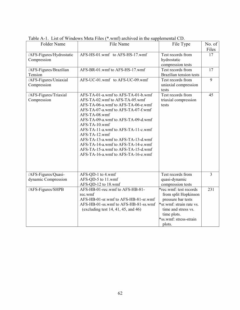
62

Table A-1. List of Windows Meta Files (*.wmf) archived in the supplemental CD.Folder Name File Name File Type No. of

Files/AFS-Figures/HydrostaticCompression

AFS-HS-01.wmf to AFS-HS-17.wmf Test records fromhydrostaticcompression tests

17

/AFS-Figures/BrazilianTension

AFS-BR-01.wmf to AFS-HS-17.wmf Test records fromBrazilian tension tests

17

/AFS-Figures/UniaxialCompression

AFS-UC-01.wmf to AFS-UC-09.wmf Test records fromuniaxial compressiontests

9

/AFS-Figures/TriaxialCompression

AFS-TA-01-a.wmf to AFS-TA-01-b.wmfAFS-TA-02.wmf to AFS-TA-05.wmfAFS-TA-06-a.wmf to AFS-TA-06-e.wmfAFS-TA-07-a.wmf to AFS-TA-07-f.wmfAFS-TA-08.wmfAFS-TA-09-a.wmf to AFS-TA-09-d.wmfAFS-TA-10.wmfAFS-TA-11-a.wmf to AFS-TA-11-c.wmfAFS-TA-12.wmfAFS-TA-13-a.wmf to AFS-TA-13-d.wmfAFS-TA-14-a.wmf to AFS-TA-14-e.wmfAFS-TA-15-a.wmf to AFS-TA-15-d.wmfAFS-TA-16-a.wmf to AFS-TA-16-e.wmf

Test records fromtriaxial compressiontests

45

/AFS-Figures/Quasi-dynamic Compression

AFS-QD-1 to 4.wmfAFS-QD-5 to 11.wmfAFS-QD-12 to 18.wmf

Test records fromquasi-dynamiccompression tests

3

/AFS-Figures/SHPB AFS-HB-01-rec.wmf to AFS-HB-81-rec.wmfAFS-HB-01-sr.wmf to AFS-HB-81-sr.wmfAFS-HB-01-ss.wmf to AFS-HB-81-ss.wmf (excluding test 14, 41, 45, and 46)

*rec.wmf: test recordsfrom split Hopkinsonpressure bar tests

*sr.wmf: strain rate vs.time and stress vs.time plots.

*ss.wmf: stress-strainplots.

231

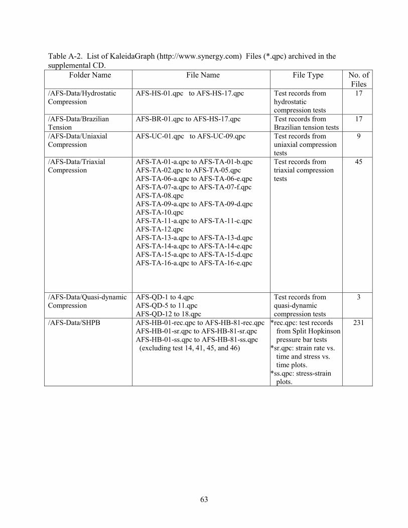
63

Table A-2. List of KaleidaGraph (http://www.synergy.com) Files (*.qpc) archived in thesupplemental CD.

Folder Name File Name File Type No. ofFiles

/AFS-Data/HydrostaticCompression

AFS-HS-01.qpc to AFS-HS-17.qpc Test records fromhydrostaticcompression tests

17

/AFS-Data/BrazilianTension

AFS-BR-01.qpc to AFS-HS-17.qpc Test records fromBrazilian tension tests

17

/AFS-Data/UniaxialCompression

AFS-UC-01.qpc to AFS-UC-09.qpc Test records fromuniaxial compressiontests

9

/AFS-Data/TriaxialCompression

AFS-TA-01-a.qpc to AFS-TA-01-b.qpcAFS-TA-02.qpc to AFS-TA-05.qpcAFS-TA-06-a.qpc to AFS-TA-06-e.qpcAFS-TA-07-a.qpc to AFS-TA-07-f.qpcAFS-TA-08.qpcAFS-TA-09-a.qpc to AFS-TA-09-d.qpcAFS-TA-10.qpcAFS-TA-11-a.qpc to AFS-TA-11-c.qpcAFS-TA-12.qpcAFS-TA-13-a.qpc to AFS-TA-13-d.qpcAFS-TA-14-a.qpc to AFS-TA-14-e.qpcAFS-TA-15-a.qpc to AFS-TA-15-d.qpcAFS-TA-16-a.qpc to AFS-TA-16-e.qpc

Test records fromtriaxial compressiontests

45

/AFS-Data/Quasi-dynamicCompression

AFS-QD-1 to 4.qpcAFS-QD-5 to 11.qpcAFS-QD-12 to 18.qpc

Test records fromquasi-dynamiccompression tests

3

/AFS-Data/SHPB AFS-HB-01-rec.qpc to AFS-HB-81-rec.qpcAFS-HB-01-sr.qpc to AFS-HB-81-sr.qpcAFS-HB-01-ss.qpc to AFS-HB-81-ss.qpc (excluding test 14, 41, 45, and 46)

*rec.qpc: test recordsfrom Split Hopkinsonpressure bar tests

*sr.qpc: strain rate vs.time and stress vs.time plots.

*ss.qpc: stress-strainplots.

231

64

DISTRIBUTION

Sandia National LaboratoriesP.O. Box 5800Albuquerque, NM 87185

MS 0841 Thomas C. Bickel (9100)MS 0751 David Bronowski (6117)MS 0751 Laurence S. Costin (6117) (2 copies)MS 0701 P. J. Davies, 6100MS 0447 Kevin Eklund (2111)MS 1174 Michael Forrestal (15414)MS 0751 Arlo Fossum (6117) (3 copies)MS 1174 Danny Frew (1174)MS 9404 John Garcia (8725)MS 0834 Justine E. Johannes (9114)MS 0847 Joseph Jung (9126)MS 0751 Moo Y. Lee (6117) (5 copies)MS 0828 Martin Pilch (9133)MS 0835 Mike McGlaun (9140)MS 0847 Harold S. Morgan (9120)MS 0824 Jaime L. Moya (9130) (3 copies)MS 0482 Robert Paulsen (2109)MS 0130 Joseph Polito (1200)MS 0824 Arthur C. Ratzel (9110)MS 0429 Steven J. Rottler (2100)MS 9003 Michael O. Vahle (9900)MS 0139 Peter J. Wilson (9902)MS0482 Joel Wirth (2131)MS0321 Paul Yarrington (9230)MS 9018 Central Tech. Files, 8945-1MS 0899 Technical Library, 9616 (2 copies)MS 0731 823/Library, 6850 (2 copies)MS 0612 Review and Approval Desk (9612)

P.O. Box 808Livermore, CA 94551

Roger Logan, L-25

65

Los Alamos National LaboratoryP.O. Box 1663Los Alamos, NM 87545

Bill Bearden MS F602Steve Girrens, ESA-EA, P946Dick Macek MS P946

Kevin C. GreenaughDepartment of Energy/Defense ProgramsDirector, Division of System Simulation & Validation1000Independence Ave., SWWashington DC 20585

Bill-Roy HarrisonDepartment of Energy/Defense ProgramsProgram Manager, Weapons Systems Engineering Certification Campaign19901 Germantown RdGermantown, MD 20874

Diane BirdWeapons Assessments and DevelopmentSupervisory General Engineer1000 Independence Ave.NA-115.1Washington DC 20585

Frozen Soil Material Testing and Constitutive...

Documents

Transcript of Frozen Soil Material Testing and Constitutive...