Frostwing Flat Plate CFD Simulations: Reynolds … · Trafi Research Report 12/2017 1 Date Title of...

Frostwing Flat Plate CFD Simulations:

Reynolds Number Effect and Boundary Layer Analysis

Pekka Koivisto, Tomi Honkanen, Juha Kivekäs

Trafi Research Reports

Trafin tutkimuksia

Trafis undersökningsrapporter 12/2017

Trafi Research Report 12/2017

1

Title of publication

Frostwing Flat Plate CFD Simulations: Reynolds Number Effect and Boundary Layer

Analysis

Author(s)

Pekka Koivisto, Tomi Honkanen, Juha Kivekäs

Commissioned by, date

Kari Wihlman, February 24th 2017

Publication series and number

Trafi Research Reports 12/2017

ISSN (online) 2342-0294

ISBN (online) 978-952-311-208-7

URN http://urn.fi/URN:ISBN:978-952-311-208-7

Keywords

CFD, aircraft, aerodynamics, de-icing fluids

Contact person

Erkki Soinne Language of the report

English

Abstract

This research report contains comparison of the flat plate CFD results to the wind tun-nel tests with matching fluid and flow properties. The research has been conducted as

part of the third year of the Frostwing project.

Three new CFD simulation cases are presented, two with a flat plate length of 0,6 m

and one with a length of 1,8 m. The cases simulate Type I de-icing fluid behavior in an accelerating air flow. The fluid properties and the acceleration of the air flow match

those present in the wind tunnel experiments used for comparison.

The latest simulation effort has two main objectives. The first is to produce simulation results that could be compared to the results of the wind tunnel experiments. The sec-

ond objective is to compare the CFD results of the 0,6-meter-long flat plate to the 1,8-meter-long version, especially the first 0,6 meters of it. This is to check if the longer

plate has an effect that propagates upstream (Reynolds number effect).

As part of the the Icewing project wind tunnel tests were also done with the flat plate models with a boundary layer pressure-rake instrumentation. A summary of the results

of these experiments are presented in this report. The boundary layer data is also

compared to the CFD results.

Date

31.7.2017


2

FOREWORD

This research report documents findings of the CFD simulations and wind tunnel experiments of de-icing fluid behavior on a flat

plate in an airstream over it. It forms part of the third year of the Frostwing project, performed under a Research agreement be-

tween the Federal Aviation Administration FAA and the Finnish Transport safety Agency Trafi together with the National Aviation

and Space Administration NASA, on the research of frost and

anti/de-icing fluid effects on aircraft wing at take-off.

The research was done by the team of Arteform Oy, headed by

MSc Juha Kivekäs.

Helsinki, July 31st 2017

Erkki Soinne

Chief Adviser, Aeronautics

Finnish Transport Safety Agency, Trafi


3

Index

Nomenclature ...................................................................................... 4

1 Background ..................................................................................... 5

2 Computational grids ........................................................................ 6

3 Description of the simulation cases ................................................. 7

4 Results ............................................................................................ 9

5 Boundary layer analysis of the flat plate wind tunnel results ........ 14

6 Comparison of the boundary layer data to the CFD results ............ 17

7 Conclusions ................................................................................... 21

References ......................................................................................... 22

Appendix I – Overview of the computational grids ............................ 23


4

Nomenclature

𝐿 flat plate length

𝑞 dynamic pressure 𝑞 = 𝜌𝑈2/2 𝑅𝑒 Reynolds number 𝑅𝑒 = 𝜌𝑈𝐿/𝜇

𝑡 time

𝑈 velocity

𝑥, 𝑦, 𝑧 coordinates

𝛿∗ boundary layer displacement thickness

𝜌 density

𝜇 dynamic viscosity note units: N∙s/m2 = kg/(m∙s) = Pa∙s = 1000 cP

𝜈 kinematic viscosity (𝜇/𝜌) note units: m2/s


5

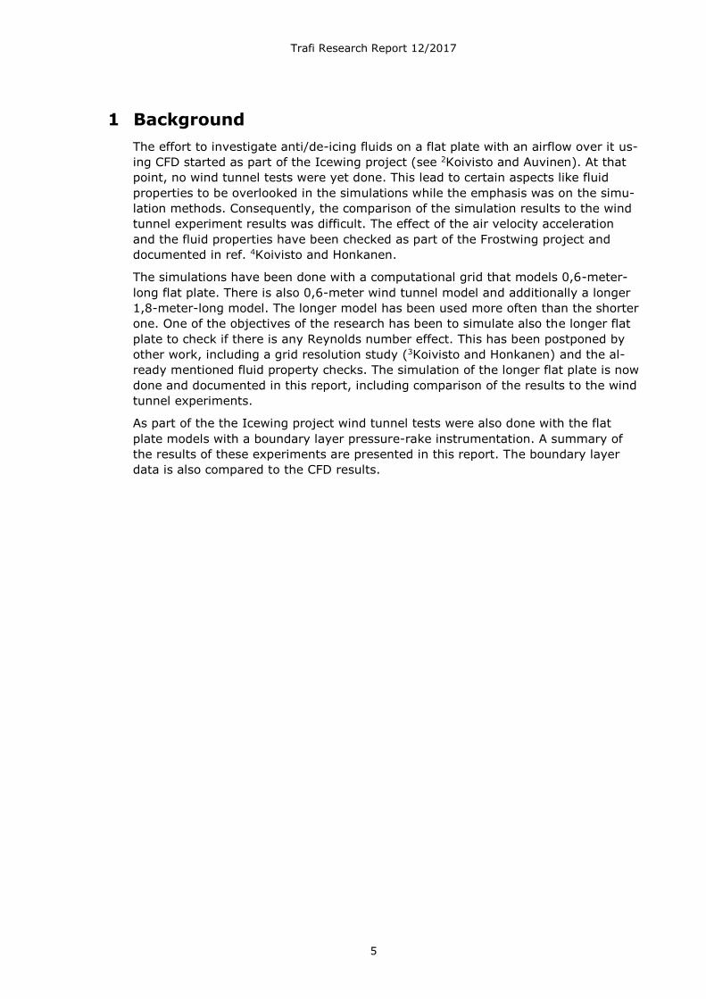
1 Background

The effort to investigate anti/de-icing fluids on a flat plate with an airflow over it us-

ing CFD started as part of the Icewing project (see 2Koivisto and Auvinen). At that

point, no wind tunnel tests were yet done. This lead to certain aspects like fluid

properties to be overlooked in the simulations while the emphasis was on the simu-

lation methods. Consequently, the comparison of the simulation results to the wind

tunnel experiment results was difficult. The effect of the air velocity acceleration

and the fluid properties have been checked as part of the Frostwing project and

documented in ref. 4Koivisto and Honkanen.

The simulations have been done with a computational grid that models 0,6-meter-

long flat plate. There is also 0,6-meter wind tunnel model and additionally a longer

1,8-meter-long model. The longer model has been used more often than the shorter

one. One of the objectives of the research has been to simulate also the longer flat

plate to check if there is any Reynolds number effect. This has been postponed by

other work, including a grid resolution study (3Koivisto and Honkanen) and the al-

ready mentioned fluid property checks. The simulation of the longer flat plate is now

done and documented in this report, including comparison of the results to the wind

tunnel experiments.

As part of the the Icewing project wind tunnel tests were also done with the flat

plate models with a boundary layer pressure-rake instrumentation. A summary of

the results of these experiments are presented in this report. The boundary layer

data is also compared to the CFD results.


6

2 Computational grids

Two computational grids have been used in the simulations covered in this report.

The original grid has been generated with GridPro software and it is 0,6 m in length

and 0,5 m in height. The grid also has depth of 1 mm in z-direction resulting in fi-

nite volume, as required in all 2D OpenFOAM simulations. This grid has been used

in vast majority of the simulations conducted in Icewing and Frostwing projects. The

total number of computational cells is approximately 160 000, of which about

80 000 are located in a refined region below the height of 60 mm.

The main issues in generating a longer version of the grid for the 1,8 m flat plate

simulations were that the GridPro software was no longer available and a com-

pletely new grid would most likely have somewhat different cell geometry in the

first 0,6 meters of length. This would lead to an uncertainty because the compari-

son of this region is the main objective. The problem was resolved by using the

OpenFOAM built-in mesh manipulation tools to generate a new longer grid by copy-

ing and mirroring the original grid. This work is documented in ref. 1Honkanen.

The new longer grid is in fact 1,76 m in length, which is 0,04 m shorter due to the

compromises involved in the generation process. This difference is however insignif-

icant considering the Reynolds number effect and other objectives. In this report,

the longer grid is labeled as 1,8 m, since this is the length of the wind tunnel model.

The longer grid has approximately 480 000 cells and has the same topology and cell

geometry as the original grid.

Overview of the computational grids is presented in Appendix I. More details and

images can be found in refs. 1Honkanen and 3Koivisto and Honkanen.


7

3 Description of the simulation cases

The latest simulation effort has two main objectives. The first is to produce simula-

tion results that could be compared to the results of the wind tunnel experiments.

This means matching the fluid properties and dynamic pressure vs. time. The sec-

ond objective is to compare the CFD results of the 0,6-meter-long flat plate to the

1,8-meter-long version, especially the first 0,6 meters of it. This is to check if the

longer plate has an effect that propagates upstream. Also, the outlet boundary con-

dition is much further away from the region of interest in this case.

Since the wind tunnel experiments with the 0,6 m and 1,8 m models were done at

different dates, they have slightly different fluid properties. This increased the num-

ber of simulation cases in order to avoid uncertainties. Total number of simulation

cases is four, including an older reference case C2. The case details are listed in Ta-

ble 1 and the air velocity ramps are presented in Figure 1.

Table 1. List of simulation cases and fluid properties.

Case Grid Air velocity

ramp

Air density

[kg/m3]

Fluid density

[kg/m3]

Fluid

viscosity

[mPas]

Surface

tension

[N/m]

C2 (ref.) 0,6 m Non-linear 1,0 1040 21 0,0298

L06A 0,6 m WT_fit 1,23 1040 33 0,036

L06B 0,6 m WT_fit 1,23 1040 49 0,036

L18 1,76 m WT_fit 1,23 1040 49 0,036

Figure 1. Comparison of the velocity ramps used as inflow boundary condition in

the CFD simulations.


8

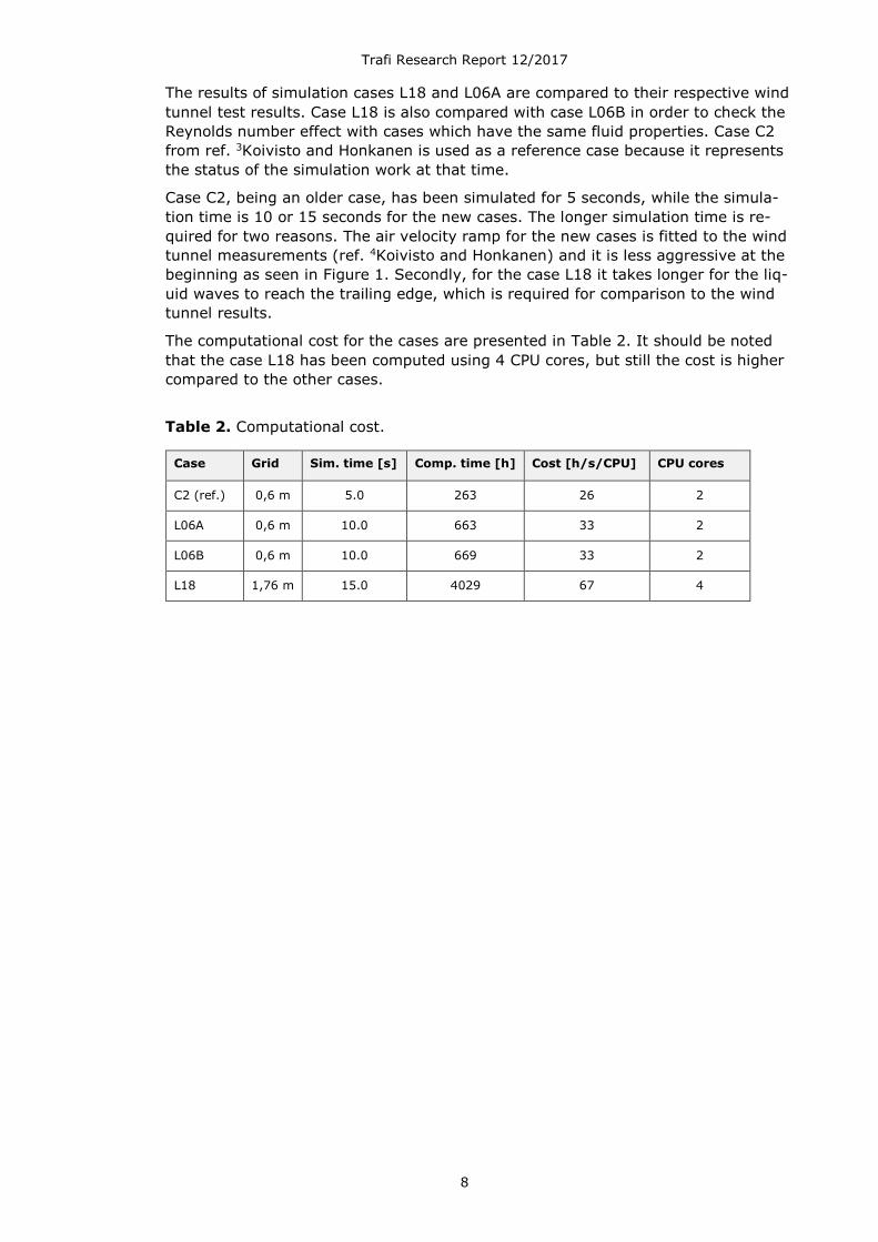
The results of simulation cases L18 and L06A are compared to their respective wind

tunnel test results. Case L18 is also compared with case L06B in order to check the

Reynolds number effect with cases which have the same fluid properties. Case C2

from ref. 3Koivisto and Honkanen is used as a reference case because it represents

the status of the simulation work at that time.

Case C2, being an older case, has been simulated for 5 seconds, while the simula-

tion time is 10 or 15 seconds for the new cases. The longer simulation time is re-

quired for two reasons. The air velocity ramp for the new cases is fitted to the wind

tunnel measurements (ref. 4Koivisto and Honkanen) and it is less aggressive at the

beginning as seen in Figure 1. Secondly, for the case L18 it takes longer for the liq-

uid waves to reach the trailing edge, which is required for comparison to the wind

tunnel results.

The computational cost for the cases are presented in Table 2. It should be noted

that the case L18 has been computed using 4 CPU cores, but still the cost is higher

compared to the other cases.

Table 2. Computational cost.

Case Grid Sim. time [s] Comp. time [h] Cost [h/s/CPU] CPU cores

C2 (ref.) 0,6 m 5.0 263 26 2

L06A 0,6 m 10.0 663 33 2

L06B 0,6 m 10.0 669 33 2

L18 1,76 m 15.0 4029 67 4


9

4 Results

The total liquid volume on the flat plate reduces as the liquid is driven off the plate

by the air flow. For the 0,6-meter flat plate results of the case L06A and the results

of Type I de-icing fluid wind tunnel tests on 7.5.2015 are compared in Figure 2. The

total liquid volume remaining in % and the dynamic pressure of the air flow in Pa x

10 are shown in the vertical axis. The horizontal axis shows time which is the same

for simulation and wind tunnel results because of the matched inflow velocity.

Since the velocity ramp and air density of 1,23 kg/m3 used in the simulations have

been matched to the wind tunnel test, the agreement of the dynamic pressure is

excellent. The fluid removal begins at about t = 4,5 s in the simulation while in the

experiment removal is observed already at t = 2,5 s. After 6 seconds of simulation

time, the simulation results and the wind tunnel test results are in excellent agree-

ment.

Figure 2. Comparison of the simulation results to the wind tunnel results for the

0,6 m flat plate (Type I fluid, date 7th May 2015).

The same velocity ramp was used in the simulation case L18 of the 1,8 m flat plate.

The results are compared to the wind tunnel test of Type I de-icing fluid on

1.4.2015 in Figure 3. There is some variation in the spool-up of the wind tunnel fan

resulting in slightly different velocity ramp profiles. The agreement of the dynamic


10

pressure in the simulation L18 and the wind tunnel tests is still very good and the

differences can be considered negligible. Similar behavior to the 0,6 m flat plate

simulation is observed, except it takes longer time (11-12 seconds) for the liquid

volume to reach the same level as in the wind tunnel test. The liquid removal be-

gins later in case L18 compared with L06A since the waves are the primary mover

of the fluid and it takes longer for the waves to reach the trailing edge in the case

L18.

Figure 3. Comparison of the simulation results to the wind tunnel results for the

1,8 m flat plate (Type I fluid, date 1st April 2015).

Several reasons for the differences between the measured and the simulated results

observed in Figures 2 and 3 can be identified:

• The initial condition in the simulations is very static, while there are initial

disturbances in the wind tunnel due to the idling of the wind tunnel fan.

• The resolution of the computational grid is insufficient to capture small

waves. The results from the grid resolution study (ref. 3Koivisto and

Honkanen) show that the removal is faster for the case with the refined grid.

• The initial thickness of the fluid was exactly 1 mm in the simulations. The in-

itial thickness of the fluid in the wind tunnel tests is more approximately de-

fined. The initial thickness has an effect on wave height and wave speed and

therefore on the removal rate.

• The waves in the simulations are formed at the leading edge of the fluid

layer and they must travel the entire plate, while waves are formed all over

the flat plate in the wind tunnel test. After the simulations have reached a

point where there are waves along the entire length of the flat plate, the re-

moval rate increases.


11

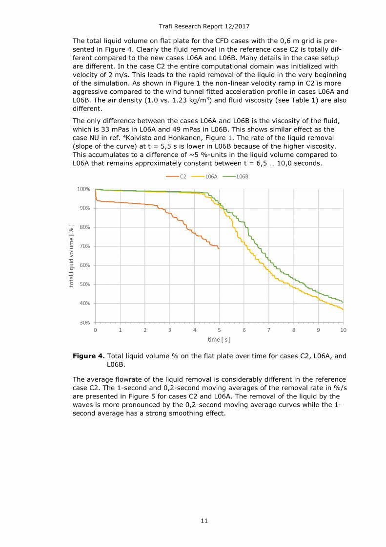
The total liquid volume on flat plate for the CFD cases with the 0,6 m grid is pre-

sented in Figure 4. Clearly the fluid removal in the reference case C2 is totally dif-

ferent compared to the new cases L06A and L06B. Many details in the case setup

are different. In the case C2 the entire computational domain was initialized with

velocity of 2 m/s. This leads to the rapid removal of the liquid in the very beginning

of the simulation. As shown in Figure 1 the non-linear velocity ramp in C2 is more

aggressive compared to the wind tunnel fitted acceleration profile in cases L06A and

L06B. The air density (1.0 vs. 1.23 kg/m3) and fluid viscosity (see Table 1) are also

different.

The only difference between the cases L06A and L06B is the viscosity of the fluid,

which is 33 mPas in L06A and 49 mPas in L06B. This shows similar effect as the

case NU in ref. 4Koivisto and Honkanen, Figure 1. The rate of the liquid removal

(slope of the curve) at t = 5,5 s is lower in L06B because of the higher viscosity.

This accumulates to a difference of ~5 %-units in the liquid volume compared to

L06A that remains approximately constant between t = 6,5 … 10,0 seconds.

Figure 4. Total liquid volume % on the flat plate over time for cases C2, L06A, and

L06B.

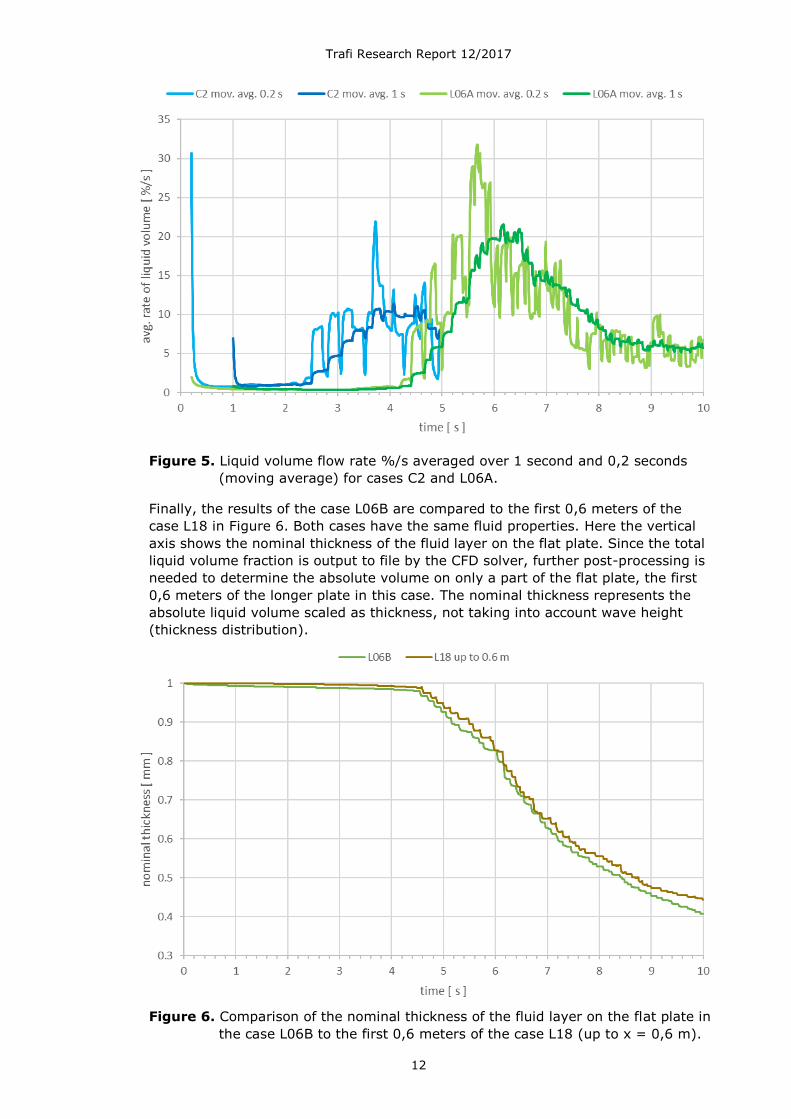
The average flowrate of the liquid removal is considerably different in the reference

case C2. The 1-second and 0,2-second moving averages of the removal rate in %/s

are presented in Figure 5 for cases C2 and L06A. The removal of the liquid by the

waves is more pronounced by the 0,2-second moving average curves while the 1-

second average has a strong smoothing effect.


12

Figure 5. Liquid volume flow rate %/s averaged over 1 second and 0,2 seconds

(moving average) for cases C2 and L06A.

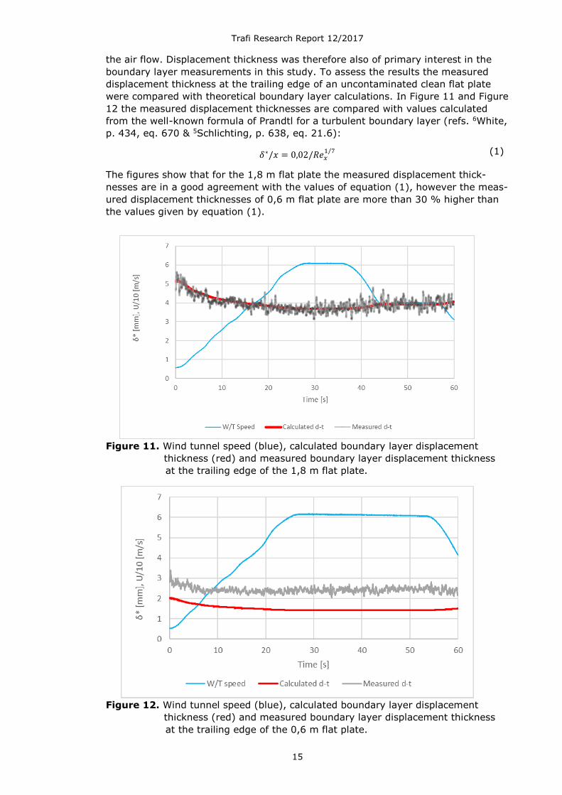
Finally, the results of the case L06B are compared to the first 0,6 meters of the

case L18 in Figure 6. Both cases have the same fluid properties. Here the vertical

axis shows the nominal thickness of the fluid layer on the flat plate. Since the total

liquid volume fraction is output to file by the CFD solver, further post-processing is

needed to determine the absolute volume on only a part of the flat plate, the first

0,6 meters of the longer plate in this case. The nominal thickness represents the

absolute liquid volume scaled as thickness, not taking into account wave height

(thickness distribution).

Figure 6. Comparison of the nominal thickness of the fluid layer on the flat plate in

the case L06B to the first 0,6 meters of the case L18 (up to x = 0,6 m).


13

Small differences can be observed in Figure 6, and the longer plate seems to add

resistance that leads to slightly less fluid to be removed than in the case L06B with

the computational domain ending at x = 0,6 m. However, the different post-pro-

cessing method used to obtain the partial volume in the case L18 could lead to inac-

curacies of the same magnitude as the difference seen in Figure 6. There are also

small qualitative differences as shown in Figure 7 which is an overview of the fluid

interface at t = 5 s.

Figure 7. Overview of the fluid interface in cases L06B, and L18 at t = 5 s,

between x = 0 … 0,6 meters.

The very slow computation of the case L18 is due to the break-up of the fluid inter-

face. The wave crests are broken and the splashes of the fluid fly in the air and hit

the fluid bed causing further disturbances. An example of this phenomenon is

shown in Figure 8 at t = 7,6 s. The break-up is problematic for the solver, because

the volume-of-fluid method used to define the phase interface in the simulation is

unable to track the rapid changes caused by the splashes.

Figure 8. Break-up of the waves in the case L18 at t = 7,6 s, between x = 0,9 …

1,2 meters.


14

5 Boundary layer analysis of the flat plate wind tunnel results

To study the effects of moving fluid layer on the boundary layer of the accelerating

airflow over it there was a boundary layer rake assembled at the trailing edge of the

flat plate as shown in Figure 9. The rake geometry is shown in Figure 10. To avoid

building a second rake for the shorter plate the rake could be tilted to a 45˚ angle

which enabled a thinner boundary layer to be measured with a reasonable accuracy.

Figure 9. Boundary layer pressure rake location on the 1,8 m flat plate wind tunnel

model. The rake is situated on the trailing edge of the shorter 0,6 m

model as shown by the arrow in the picture.

Figure 10. Boundary layer rake tube geometry at 90˚ angle. Topmost tube is the

static pressure reference.

To avoid the moving fluid to clog the lowest pitot tubes they were sealed. For the

0,6 m plate the 4 lowest tubes were sealed whereas for 1,8 m plate the 6 lowest

tubes were sealed. When calculating the boundary layer thickness the pitot pressure

at the lowest tubes had to be extrapolated using the data from the open tubes. This

naturally includes an unknown error source.

In the de/anti-icing aerodynamic acceptance test (SAE AS 5900) the fluid aerody-

namic effect is defined by measuring the boundary layer displacement thickness of

Rake on 0,6 m

model


15

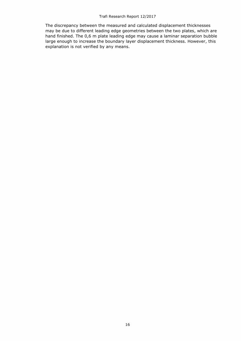
the air flow. Displacement thickness was therefore also of primary interest in the

boundary layer measurements in this study. To assess the results the measured

displacement thickness at the trailing edge of an uncontaminated clean flat plate

were compared with theoretical boundary layer calculations. In Figure 11 and Figure

12 the measured displacement thicknesses are compared with values calculated

from the well-known formula of Prandtl for a turbulent boundary layer (refs. 6White,

p. 434, eq. 670 & 5Schlichting, p. 638, eq. 21.6):

𝛿∗/𝑥 = 0,02/𝑅𝑒𝑥

1/7 (1)

The figures show that for the 1,8 m flat plate the measured displacement thick-

nesses are in a good agreement with the values of equation (1), however the meas-

ured displacement thicknesses of 0,6 m flat plate are more than 30 % higher than

the values given by equation (1).

Figure 11. Wind tunnel speed (blue), calculated boundary layer displacement

thickness (red) and measured boundary layer displacement thickness

at the trailing edge of the 1,8 m flat plate.

Figure 12. Wind tunnel speed (blue), calculated boundary layer displacement

thickness (red) and measured boundary layer displacement thickness

at the trailing edge of the 0,6 m flat plate.


16

The discrepancy between the measured and calculated displacement thicknesses

may be due to different leading edge geometries between the two plates, which are

hand finished. The 0,6 m plate leading edge may cause a laminar separation bubble

large enough to increase the boundary layer displacement thickness. However, this

explanation is not verified by any means.


17

6 Comparison of the boundary layer data to the CFD re-sults

Boundary layer data of the Type I anti-icing wind tunnel test of 7th May 2015 is

compared with the CFD case L06A which has been simulated with the same flow

properties. The CFD result data has been saved at 0,005 second intervals, matching

the rake measurement frequency of 200 Hz. The velocity data is probed from same

locations as the boundary layer rake tubes were on the wind tunnel model. The ve-

locity profile is averaged over t = 7,0 … 7,2 seconds in the CFD simulation and

therefore it consists of 40 time samples. The inflow velocity is approximately 22,5 –

23 m/s (q ≈ 310 Pa) at this time interval.

The measured velocity profiles at the trailing edge (x = 0,585 m from the leading

edge) are presented in Figure 13. Included are one dry wind tunnel run without

fluid, two runs with fluid (same runs as in Figure 2). Note that the air velocity in

two points nearest of the wall are not measured (distance from the wall 0 and

0,18) and in the four next points from the wall are extrapolated values as the

pitot tubes have been sealed.

Figure 13. Comparison of the measured velocity profiles at the trailing edge of the

0,6 m flat plate (x = 0,585 m from the leading edge).

Figure 14 shows comparison of the mean value of the CFD calculations of the case

L06A between time period t = 7…7,2 s to the wind tunnel runs. The shape of CFD

mean velocity profile differs significantly from the measured ones.


18

Figure 14. Measured velocity profiles for the two fluid runs compared to mean

velocity profile of the CFD case L06A over time period t = 7…7,2 s.

There are strong fluctuations in the CFD velocity due to the air vortices. This is visi-

ble in the mean CFD velocity curve which shows a higher velocity in the y = 10 mm

region compared to the free flow. To illustrate these fluctuations Figure 15 and Fig-

ure 16 show the velocity profile combined with the corresponding wave positions at

time instants t = 7,08 s and 7,125 s. The vicinity of the wave seems to intensify the

effect of a vortex on the velocity profile.


19

Figure 15. Measured velocity profiles compared to CFD velocity profiles at time

points t = 7,08 s and 7,125 s.

Figure 16. Velocity calculation line at x = 0,585 m (”probe position”) relative to

wave positions at time instants t = 7,08 and 7,125 s.

Velocity

probe line


20

The displacement thicknesses calculated from velocity profiles of Figure 14 are:

• wind tunnel run 1 (@ ~23 m/s): δ* = 4,0 mm

• wind tunnel run 2 (@ ~23 m/s): δ* = 4,7 mm

• CFD mean velocity (@ 7…7,2 s, ~23 m/s): δ* = 3,0 mm

There are many potential reasons for large deviations between measured and CFD

simulation results within the boundary layer:

• 2D LES model with SGS – model may fail in results in the boundary layer

near the wall (in this case near the fluid layer).

• The CFD computational grid may not be optimal for boundary layer calcula-

tions.

• Pitot tube measurements act as an efficient filter for frequencies higher than

10 to 100 Hz while the calculated fluctuations are at frequencies of one to

two orders of magnitude higher.

• The presence of the rake assembly could interfere with the air vortices mak-

ing their measurement difficult.

• Since the pitot tubes of the rake are designed to measure total pressure of

the flow in direction approximately parallel to the tubes, it is questionably if

measurement of the vortex street is possible due to the large variations in

the local flow direction.

• Considering the differences between measurements for uncontaminated 0,6

m and 1,8 m flat plates the 0,6 m plate results are worse when compared to

analytical solutions. The reason for this remains unknown.


21

7 Conclusions

The case L06A has been simulated with matching fluid and flow properties to pro-

duce simulation results that would be fully comparable to the wind tunnel experi-

ments. The fluid flow-off results are in very good agreement. The longer 1,8 m flat

plate has been simulated for the first time (case L18). The simulation was very time

consuming but eventually after 12 seconds of simulation time the total volume

reached the same level as in the measurements. From this point until the end of the

simulation at 15 seconds, the agreement with the measurements is very good.

Overall the shape of the flow-off curve is similar between the 0,6 m and the 1,8 m

cases. There is a similarly slow flow rate to be observed in the beginning of the case

L18 as in the case L06A, and the case L06B with fluid properties of L18. There are

still uncertainties that could explain this phenomenon, including the instability of the

measured liquid due to wind tunnel idling compared to the mathematically accurate

steady initial condition in the simulations. In the simulations the waves are formed

at the leading edge only and they must travel longer distance from the leading edge

to the trailing edge in the case L18.

Any upstream effect of the higher Reynolds number was deemed negligible when

the first 0,6 meters of the longer case were compared to the case L06B. This sug-

gests that the outlet boundary condition does not have a negative effect in the sim-

ulations.

The comparison of the measured boundary layer rake results to the simulations

proved challenging. The velocity was probed directly from the simulations while dy-

namic pressure was measured using the rake. Even though the sampling frequency

was 200 Hz in both simulations and measurements, the air vortices are clearly visi-

ble only in the CFD velocity profiles. The air vortices are strong and frequent

enough to distort the mean velocity profile. A longer sampling time could be used,

but the accelerating air flow adds another uncertainty in this case.


22

References

1Honkanen T., Generating a longer flat plate computational grid, Arteform

memorandum, 29 Mar 2016, 11 p.

2Koivisto P. and Auvinen M., Preliminary CFD Investigation of De/anti-icing Fluid

Behavior on a Flat Plate, Trafi Research Report 5/2015, 2015, 18 p.

3Koivisto P. and Honkanen T., Grid Resolution and Parameter Sensitivity Study of Flat

Plate CFD Simulations, Trafi Research Report 4/2016, 2016, 42 p.

4Koivisto P. and Honkanen T., Technical Reports on Frostwing Flat Plate CFD

Simulations, Trafi Research Report 7/2017, 26 p.

5Schlichting H., Boundary-Layer Theory, 7th Edition, McGraw-Hill, 1979, 817 p.

6White F. M., Viscous Fluid Flow, McGraw-Hill, 1991, 614 p.


Appendix I – Overview of the computational grids

Figure 17. Overview of the original 0,6-meter flat plate grid with approximately 160 000 cells.

0,6 m

0,5 m


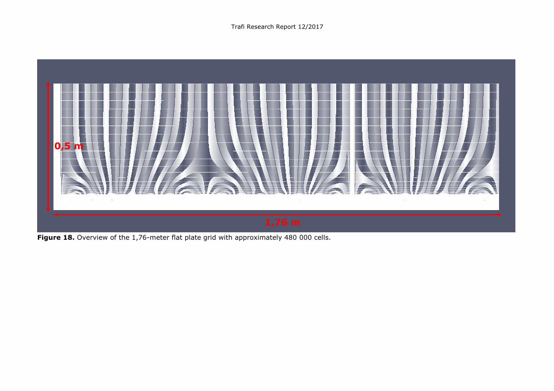
Figure 18. Overview of the 1,76-meter flat plate grid with approximately 480 000 cells.

1,76 m

0,5 m

Frostwing Flat Plate CFD Simulations: Reynolds … · Trafi Research Report 12/2017 1 Date Title of...

Documents

Transcript of Frostwing Flat Plate CFD Simulations: Reynolds … · Trafi Research Report 12/2017 1 Date Title of...