From Ruin Theory to Option Pricing

Hans U. Gerber Ecole des hautes ttudes cornmerciales

Universitt de Lausanne CH- 1015 Lausanne. Switzerland

Phone: 41 21 692 3371 Fax: 41 21 692 3305

E-mail: hgerber@hec.unil.ch

Elias S.W. Shiu Department of Statistics and Actuarial Science

The University of Iowa Iowa City, Iowa 52242, U.S.A.

Phone: 319 335 2580 Fax: 319 335 3017

E-mail: eshiu8stat.uiowa.edu

Abstract We examine the joint distribution of the time of ruin, the surplus immediately

before ruin, and the deficit at ruin. The time of ruin is analyzed in terms of its Laplace

transform, which can naturally be interpreted as discounting. We show how to

calculate an expected discounted penalty, which is due at ruin, and may depend on the

deficit at ruin and the surplus immediately before ruin. The expected discounted

penalty, considered as a function of the initial surplus, satisfies a certain renewal

equation. By replacing the penalty at ruin with a payoff at exercise, these results can

be applied to price a perpetual American put option on a stock, where the logarithm of

the stock price is a shifted compound Poisson process. Because of the stationary

nature of the perpetual option, its optimal option-exercise boundary does not vary with

respect to the time variable. We have derived an explicit formula for determining the

optimal boundary.

Keywords Collective risk theory, compound Poisson process, surplus process, ruin probability,

severity of ruin, deficit at ruin, time of ruin, adjustment coefficient, Lundberg's

fundamental equation, Laplace transforms, renewal equation, martingales, optional

sampling theorem, stopping time, perpetual American options, put options,

continuous junction.

De la thdorie de la ruine B l'kvaluation du prix d'une option

Hans U. Gerber Ecole des hautes ttudes commerciales

Universitt de Lausanne CH-1015 Lausanne, Suisse

Phone: 41 21 692 3371 Fax: 41 21 692 3305

E-mail: hgerber@hec.unil.ch

Elias S.W. Shiu Department of Statistics and Actuarial Science

The University of Iowa Iowa City, Iowa 52242, U.S.A.

Phone: 3 19 335 2580 Fax: 319 335 3017

E-mail: eshiu@stat.uiowa.edu

R&umC Nous examinons la distribution conjointe du temps de la mine, du surplus juste

avant la mine et du dtficit au moment de la ruine. Le temps de la mine est analyst par sa

transformte de Laplace, qui peut &tre interpdtte comme une valew escomptte. Nous

montrons comment calculer l'esptrance mathtmatique de la valew escompt6e d'un certain

paiement, qui est dCi au moment de la mine, et qui peut &me une fonction du dtficit et du

surplus juste avant la mine. Cette esphance mathtmatique, considtrte comme fonction

du surplus initial, est solution d'une certaine tquation de renouvellement. En interpretant

le paiement comrne le payoff & la date d'exercice, nous pouvons appliquer les rtsultats

pow dtterminer le prix d'une option de vente peqdtuelle; dans le modele, le prix de

l'action sous-jacente est un processus de Poisson compost avec dkalage. A cause de la

stationnaritk du modble et du payoff, la frontikre d'exercice optimale ne varie pas dans le

temps. Nous indiquons une formule explicite pow dtterminer cette frontibre optimale.

Mots clefs Thtorie du risque collectif, processus de Poisson compost, processus de surplus,

probabilitt de la mine, stvtritt de la mine, dtficit au moment de la mine, temps de la

mine, coefficient d'ajustement, tquation de Lundberg, transformte de Laplace,

Quation de renouvellement, martingales, thtorbme d'arrEt, temps d'arrEt, options

amtricaines perpttuelles, option de vente, jonction continue

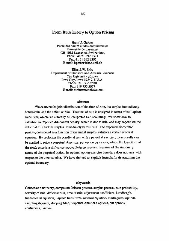
1. Introduction Collective risk theory has started in 1903 with the doctoral thesis of Filip

Lundberg, a Swedish actuary, and it has been developed throughout this century. It is

now an area rich in useful ideas and sophisticated techniques. Many of its tools can be

applied to solve problems in other fields. A recent example is the method of Esscher

transform, which was used by Gerber and Shiu (1994a, 1994b. 1996b) to price

financial derivatives.

Two particular questions of interest in collective risk theory are (a) the deficit

a t ruin, and (b) the time of ruin, both of which have been treated separately in the

literature. In this paper the two questions are combined. From a mathematical point

of view, a crucial role is played by the amount of surplus immediately before ruin

occurs. Hence we examine the joint distribution of three random variables: the

surplus immediately before ruin, the deficit at ruin, and the time of ruin. The time of

ruin is analyzed in terms of its Laplace transform, which can naturally be interpreted

as discounting. We obtain results for the joint distribution by studying the expectation

of a discountedpenalty, which is due at ruin and depends on the deficit at ruin and the

surplus immediately prior to ruin. The expected discounted penalty, considered as a

function of the initial surplus, satisfies a certain renewal equation.

This paper generalizes and adds to a better understanding of classical ruin

theory, which we can retrieve by setting the force of interest (Laplace transform

variable) equal to zero. For example, in the classical model, the adjustment

coeficient is the solution of an implicit equation, which has 0 as the other solution. If

the interest rate is positive, the situation is suddenly symmetric: the corresponding

equation, called Lundberg 'sfitndamental equation, has a positive solution and a

negative solution. Both solutions are important and are used to construct exponential

martingales.

This paper was motivated by the problem of pricing perpetual American

options. The classical model uses the geometric Brownian motion to model the stock

price process. Such a process has continuous sample paths, which facilitate the analysis

of an American option: the option is exercised as soon as the stock price anives on the

optimal exercise boundary, and the price of the option is the expected discounted payoff

(Gerber and Shiu 1994b, 1996a). On the other hand, we would like to price an American option in a perhaps more realistic model where the stock price may have

jumps, for example drops. The resulting mathematical problem is more intricate,

because now, at the time of the exercise, the stock price is not on but beyond the

optimal exercise boundary. If the logarithm of the stock price is modeled by a shifted

compound Poisson process, this leads to the type of problems that are discussed in the

earlier part of the paper, with "penalty at ruin" replaced by "payoff at exercise."

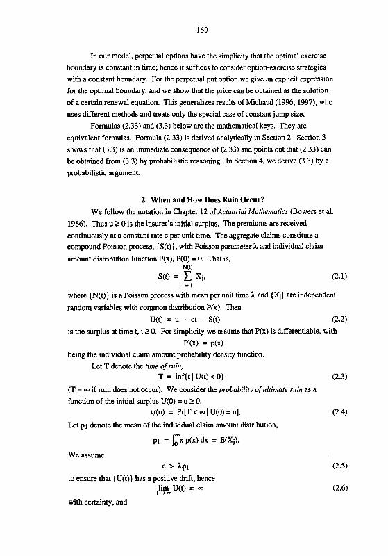
In our model, perpetual options have the simplicity that the optimal exercise

boundary is constant in time; hence it suffices to consider option-exercise strategies

with a constant boundary. For the perpetual put option we give an explicit expression

for the optimal boundary, and we show that the price can be obtained as the solution

of a certain renewal equation. This generalizes results of Michaud (1996, 1997), who

uses different methods and treats only the special case of constant jump size.

Formulas (2.33) and (3.3) below are the mathematical keys. They are

equivalent formulas. Formula (2.33) is derived analytically in Section 2. Section 3

shows that (3.3) is an immediate consequence of (2.33) and points out that (2.33) can

be obtained from (3.3) by probabilistic reasoning. In Section 4, we derive (3.3) by a

probabilistic argument.

2. When and How Does Ruin Occur? We follow the notation in Chapter 12 of Actuarial Mathematics (Bowers et al.

1986). Thus u 1 0 is the insurer's initial surplus. The premiums are received

continuously at a constant rate c per unit time. The aggregate claims constitute a compound Poisson process, {S(t)), with Poisson parameter h and individual claim

amount distribution function P(x), P(0) = 0. That is, N(t)

= C xj* (2.1) j = 1

where [N(t)] is a Poisson process with mean per unit time h and [Xj] are independent

random variables with common distribution P(x). Then

U(t) = u + ct - S(t)

is the surplus at time t, t t 0. For simplicity we assume that P(x) is differentiable, with

p'(x) = p(x) being the individual claim amount probability density function.

Let T denote the time of ruin, T = inf[t I U(t) < 0)

(T = m if ruin does not occur). We consider the probability of ultimate ruin as a

function of the initial surplus U(0) = u 2 0, ~ ( u ) = h[T < m I U(0) = u].

Let pi denote the mean of the individual claim amount distribution,

We assume

c > h ~ l to ensure that {U(t)] has a positive drift; hence

lirn U(t) = m t+-

with certainty, and

v(u) 1. (2.7) Condition (2.5) is a natural assumption in the context of ruin theory; however, it is not

crucial for the mathematical development in this paper.

We also consider the random variables U(T-), the surplus immediately before

ruin, and U(T), the surplus at ruin. See Figure 1 . For given U(0) = u 2 0, let f(x, y, t I u) denote the joint probability density function of U(T-), IU(T)I and T. Then

j ~ j , " ~ ~ f ( x , y. t 1 U) dxdydt = R[T c - 1 U(0) = U] = ~ ( u ) . (2.8)

Because of (2.7), f(x, y, t ( u) is a defective probability density function. We remark

that, for x > u + ct,

f(x, y, tl U) = 0,

and that f(u+ct, y, t 1 U) dxdydt = e-%p(u+ct+y)dydt.

Figure 1. The Surplus Immediately before and at Ruin

It is easier to analyze the following function, the study of which is a central theme in this paper. For 6 2 0, define

f(x, y I U) = Ite-&f(x, y, t I u) dt. (2.9)

Here 6 can be interpreted as a force of interest, or, in the context of Laplace transforms, as a dummy variable. For notational simplicity, the symbol f(x, y I u) does

not exhibit the dependence on 6. If 6 = 0, (2.9) is the defective joint probability

density function of U(T-) and IU(T)I, given U(0) = u. Also, if 6 > 0, then

e a = e* I(T < m),

where I denotes the indicator function, i.e., I(A) = 1 if A is true and I(A) = 0 if A is

false.

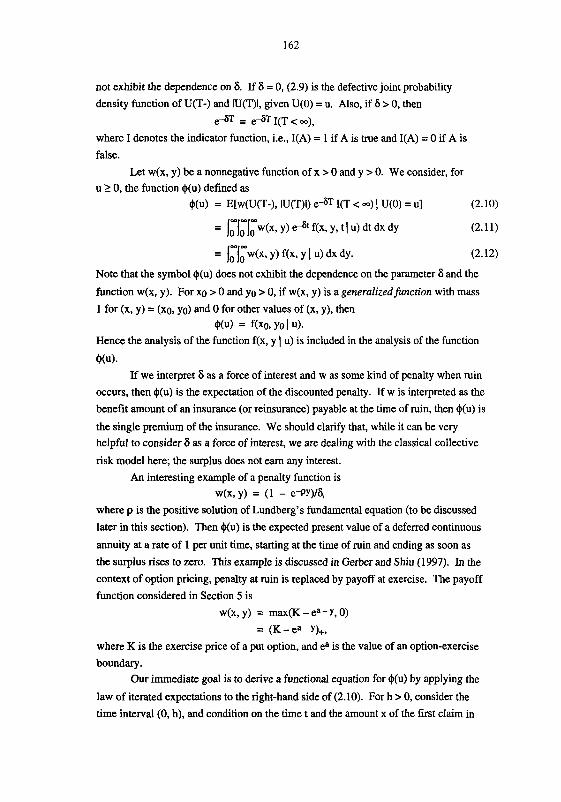
Let w(x, y) be a nonnegative function of x > 0 and y > 0. We consider, for u 1 0 , the function $(u) defined as

$(u) = E[w(U(T-), IU(T)I) e-6T I(T < m) ] U(0) = u] (2.10)

= / l l iw(x, y) f(x, y I U) dx dy. (2.12)

Note that the symbol $(u) does not exhibit the dependence on the parameter 6 and the

function w(x, y). For xg > 0 and yo > 0, if w(x, y) is a generalizedfunction with mass

1 for (x, y) = (xo, yo) and 0 for other values of (x, y), then

4 0 ) = f(x0. yo I u). Hence the analysis of the function f(x, y I u) is included in the analysis of the function

Mu). If we interpret 6 as a force of interest and w as some kind of penalty when ruin

occurs, then $(u) is the expectation of the discounted penalty. If w is interpreted as the

benefit amount of an insurance (or reinsurance) payable at the time of ruin, then $(u) is

the single premium of the insurance. We should clarify that, while it can be very helpful to consider 6 as a force of interest, we are dealing with the classical collective

risk model here; the surplus does not earn any interest.

An interesting example of a penalty function is W(X, y) = (1 - e-PY)I&

where p is the positive solution of Lundberg's fundamental equation (to be discussed

later in this section). Then $(u) is the expected present value of a deferred continuous

annuity at a rate of 1 per unit time, starting at the time of ruin and ending as soon as

the surplus rises to zero. This example is discussed in Gerber and Shiu (1997). In the

context of option pricing, penalty at ruin is replaced by payoff at exercise. The payoff

function considered in Section 5 is

W(X, y) = max(K-ea-Y,0)

= (K-ea-Y),,

where K is the exercise price of a put option, and ea is the value of an option-exercise

boundary. Ow immediate goal is to derive a functional equation for $(u) by applying the

law of iterated expectations to the right-hand side of (2.10). For h > 0, consider the

time interval (0, h), and condition on the time t and the amount x of the first claim in

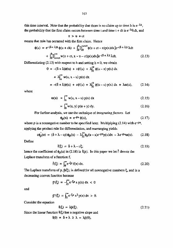
this time interval. Note that the probability that there is no claim up to time h is e-hh, the probability that the first claim occurs between time t and time t + dt is e-%dt, and

X > U +Ct

means that ruin has occurred with the first claim. Hence h u+ct

$(u) = e-@+ $(u + ch) + lo [IO $(u + ct - ~ ) ~ ( x ) d x ] e < ~ + l ) t hdt

+ %[ltKtw(u + ct, x - u - ~t)~(x)dx]e-@+ hdt.

Differentiating (2.13) with respect to h and setting h = 0, we obtain

0 = 4 6 + h)$(u) + c$'(u) + q: $(u - X) p(x) dx

where

= /:w(u, Y) ~ ( u + Y) dy. (2.16)

For further analysis, we use the technique of integrating factors. Let

$p(u) = e-PU $W, (2.17) where p is a nonnegative number to be specified later. Multiplying (2.14) with e-PU,

applying the product rule for differentiation, and rearranging yields

@L(u) = (6 + h - C ~ ) $ ~ ( U ) - h c $ P ( ~ - x)e-Pxp(x)dx - he-Puo(u). (2.18)

Define P(5) = 6 + h - 4 ; (2.19)

hence the coefficient of $&) in (2.18) is P(p). In this paper we let ? denote the

Laplace transform of a function f,

T(Q = /;e+ f(x) dx. (2.20)

The Laplace transform of p, @(5), is defined for all nonnegative numbers 5, and is a

decreasing convex function because

~'(5) = -lie+ x P(X) dx < o and

~ " ( 5 ) = l ie+ x2 p(x) dx > 0.

Consider the equation

P(5) = @(GI. Since the linear function P(6) has a negative slope and

P(0) = 6 + h 2 h = @(0),

equation (2.21) has a unique nonnegative root, say tl. Furthermore, if the individual

claim amount density function p is sufficiently regular, equation (2.21) has one more root, say t2, which is negative. This negative root will be denoted as -R. As we shall

see in Section 4, both roots are related to the construction of exponential martingales. When 6 = 0, R is the adjustment coeficient in classical risk theory. Equation (2.21) is

equivalent to Beekman (1974, p. 41, top equation), Panjer and Willmot (1992, Eq.

11.7.8), and Seal (1969, Eq. 4.24). Lundberg (1932, p. 144) points out that the

equation is "fundamental to the whole of collective risk theory," and Seal (1969, p.

I l l ) calls it "Lundberg's (1928) 'fundamental' equation." [Seal (1969, p. 112) asserts

incorrectly that the second root is also positive.]

The trick for solving (2.18) is to choose

P = 51% (2.22) so that (2.18) becomes

4&4 = A#Kp)bp(u) - h/;$p(u - x)e-Pxp(x)dx - he-PUO(u)

For z > 0, we integrate (2.23) from u = 0 to u = z. After a division by h, the resulting

equation is

39p(z) - cPP(O)l

= fi(p)ji(p(~)du - Ii[c $p(x)e-P(u-x+(u - x)dx]du - lie-Puw(u)du

= fi(p$(p(u)du - I;[/;e+(~-~)p(u - x)d~](~(x)dx - ce+uw(u)du

= /i4p(x)[jzIx e-PYp(y)dy]dx - \;e-P"w(u)du. (2.24)

For z + -, the first terms on both sides of (2.24) vanish, which shows that

h " h Op(0) = r lo e+uo(u)du = r Q(p).

Substituting (2.25) in (2.24) and simplifying yields

= $ { ~ ~ $ p ( x ) ~ ~ ~ x e * ~ ( ~ ) d ~ ~ ~ + /re+uo(u)du), z 2 0. (2.26)

Multiplying (2.26) with ePZ and applying (2.17), we have

((z) = $ { C ( ( X ) [ ] ~ ~ ~ P ( T X - Y ) ~ ( ~ ) ~ ~ ] ~ X + l f e~(~)co(u)du) . (2.27)

For two integrable functions fl and f2 defined on [0, m), the convolution of fl

and f2 is the function

(f~*fi)(x) = l ifdy) f2(x - Y) d ~ , x 2 0 . (2.28)

Note that fl*f2 = f2*fl.

With the definitions

and

h(x) = h jme+(u-X) MU) du c x (2.31)

- h -- - Ix IO e+(u-~) w(u, y) p(u + y) dy du, x 2 0, (2.32)

equation (2.27) can be written more concisely as

@ = g*g + h. (2.33)

In the literature of integral equations, (2.33) is classified as a Volterra equation of the

second kind. The function g is a nonnegative function on [0, m) and hence may be

interpreted as a (not necessarily proper) probability density function; in probability theory, (2.33) is known as a renewal equation for the function g.

The solution of (2.33) can be expressed as an infinite series of functions,

sometimes called a N e m n n series, 41 = h + g*h + g*g*h + g*g*g*h + g*g*g*g*h + ... . (2.34)

One may obtain (2.34) from (2.33) by the method of successive substitution.

Remarks (i) It follows from the conditional probability formula,

Pr(A n B) = MA) Pr(B 1 A),

that the joint probability density function of Up-), IU(T)I and T at the point (x, y, t) is

the joint probability density function of Up-) and T at the point (x, t) multiplied by the

conditional probability density function of IU(T)I at y, given that U(T-) = x and T = t. The latter does not depend on t and is

f(x I U) = I ~ ( X , Y l U) dy

= /J:e* f(x, Y, t I u) dt dy,

multiplying (2.35) with e4t and then integrating with respect to t yields

P(x+y) f ( x , ~ I u ) = f(xIu)=. (2.37)

With 6 = 0, (2.37) was pointed out by Dufresne and Gerber (1988, Eq. 3); another

proof can be found in Dickson and Egidio dos Reis (1994).

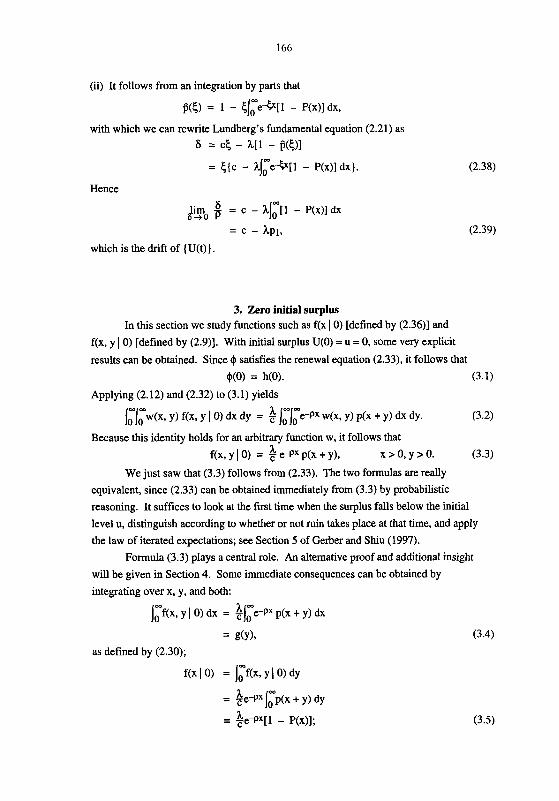
(ii) It follows from an integration by parts that

~ ( 5 ) = 1 - E,\;e-5.[1 - P(X)J dx,

with which we can rewrite Lundberg's fundamental equation (2.21) as s = CS - n[i - fig)]

= $(c - $'e-b[l - ~ ( x ) l d x ~ .

Hence

pio 8 = c - h];[l - P(x)J dx

= c - hpl,

which is the drift of {U(t) 1.

3. Zero initial surplus In this section we study functions such as f(x I 0) [defined by (2.36)] and

f(x, y 1 0) [defined by (2.9)]. With initial surplus U(0) = u = 0, some very explicit

results can be obtained. Since 4 satisfies the renewal equation (2.33), it follows that

4(0) = W ) . (3.1)

Applying (2.12) and (2.32) to (3.1) yields

]J;w(x, y) f(x. Y I 0) dx dy = /;\;e-~x w(x. r) P(X + Y) dx dy. (3.2)

Because this identity holds for an arbitrary function w, it follows that h f(x, y 1 0) = e-Px p(x + y), x>O,y>O. (3.3)

We just saw that (3.3) follows from (2.33). The two formulas are really

equivalent, since (2.33) can be obtained immediately from (3.3) by probabilistic

reasoning. It suffices to look at the first time when the surplus falls below the initial

level u, distinguish according to whether or not ruin takes place at that time, and apply

the law of iterated expectations; see Section 5 of Gerber and Shiu (1997).

Formula (3.3) plays a central role. An alternative proof and additional insight

will be given in Section 4. Some immediate consequences can be obtained by

integrating over x, y, and both:

/;f(x, y 1 01 dx = $];e+x p(x + y) dx

= g(y), as defined by (2.30);

f(x I 0) = /tf(x, Y I 0) dy

= $e.+~/;~(p(x + y) dy

h = Fe+X[l - P(x)];

= $I;e+[l - P(x)] dx. (3.6)

As a check, note that (3.3) and (3.5) satisfy (2.37) with u = 0. With 6 = 0, and hence p = 0, (3.3) reduces to a result of Dufresne and Gerber

(1988, Eq. 10). In particular,

f(x. Y 10) = f(y, x 10). (3.7)

Dickson (1992) has pointed out that this symmetry can be explained in terms of

duality. Further discussion can be found in Dickson and Egidio dos Reis (1994), and Gerber and Shiu (1997). For 6 > 0, formula (3.7) does not hold any longer.

For 6 = 0, (3.6) reduces to the famous formula

~ ( 0 ) = $/;[I - P(x)] dx

= hpl/c. (3.8)

For 6 > 0, we can use (3.6) and the fact that p is a solution of (2.38) to see that E[e-GT I U(0) = 01 = em I(T < m) I U(0) = 0]

- - 1 - q y 6 (3.9)

Formula (3.8) can be obtained as a limiting case of (3.9) because of (2.39).

Example Let us look at the case of an exponential individual claim amount

distribution, p(x) = pe-b, x 2 0, (3.10)

h with p > 0 and c > hpl = p. The number p is el, the nonnegative solution of (2.21),

which now is

Hence

(Note that, if 6 = 0, then p = $1 = 0.) Then

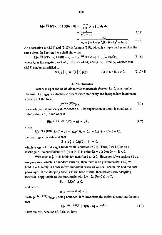
An alternative to (3.14) and (3.15) is formula (3.9). which is simple and general at the

same time. In Section 4 we shall show that E[eAT I(T < m) I U(0) = u] = E[eAT I(T < m) I U(0) = 0] etzu, (3.16)

where (2 is the negative root of (3.1 1); see (4.14) and (4.19). Finally, we note that

(2.37) can be simplified to

f(x. Y 1 u) = f(x 1 u) P(Y), u l o , x > 0, y > 0. (3.17) 1111

4. Martingales Further insight can be obtained with martingale theory. Let ( be a number.

Because {U(t)}m is a stochastic process with stationary and independent increments,

a process of the form i e 4 t + tU(0 )

is a martingale if and only if, for each t > 0, its expectation at time t is equal to its

initial value, i.e., if and only if

E[eAt + tu(t) I U(0) = U] = e b . (4.2)

Since E[e-6t + 5U(t) I U(0) = u] = exp(-& + (u + (ct + kt@(() - 11).

the martingale condition is that -6 + C( + A[$(() - I] = 0,

which is again Lundberg's fundamental equation (2.21). Thus, for (4.1) to be a martingale, the coefficient of U(t) in (4.1) is either k1 = p l 0 or (2 = -R < 0.

With such a 5, (4.2) holds for each fixed t, t 2 0. However, if we replace t by a

stopping time which is a random variable, then there is no guarantee that (4.2) will

hold. Fortunately, it holds in two important cases, as we shall see in this and the next

paragraph. If the stopping time is T, the time of ruin, then the optional sampling theorem is applicable to the martingale with ( = -R. For 0 5 t < T,

6t + R u t ) 2 0,

and hence 0 < e-St- W t ) 5 1.

With {eAt-Ru(t))wttcr being bounded, it follows from the optional sampling theorem

that ~ [ e d T - RU(T) I U(0) = u] = e-RU . (4.3)

Furthermore, because of (2.6). we have

E[eAT - RU(T) I(T = m) I U(0) = u] = 0

even if 6 = 0. Consequently, we can rewrite (4.3) as

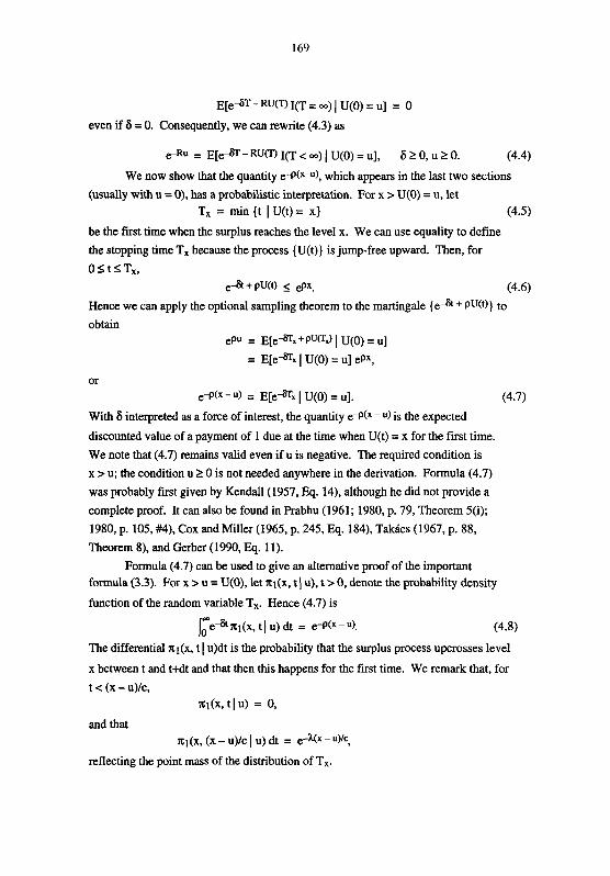
We now show that the quantity e-P(x-u), which appears in the last two sections

(usually with u = O), has a probabilistic interpretation. For x > U(0) = u, let Tx = min ( t I U(t) = x} (4.5)

be the first time when the surplus reaches the level x. We can use equality to define

the stopping time T, because the process {U(t)) is jump-free upward. Then, for

OStSTx, e-6t + PW < &x. (4.6)

Hence we can apply the optional sampling theorem to the martingale {edt + Pu(t)) to

or e+(x - U) = E [ e a ~ I U(0) = u]. (4.7)

With 6 interpreted as a force of interest, the quantity e-P(x- u) is the expected

discounted value of a payment of 1 due at the time when U(t) = x for the first time.

We note that (4.7) remains valid even if u is negative. The required condition is

x > u; the condition u 2 0 is not needed anywhere in the derivation. Formula (4.7)

was probably first given by Kendall(1957, Eq. 14), although he did not provide a

complete proof. It can also be found in Prabhu (1961; 1980, p. 79, Theorem 5(i);

1980, p. 105, #4), Cox and Miller (1965, p. 245, Eq. 184), Takacs (1967, p. 88,

Theorem 8), and Gerber (1990, Eq. 11).

Formula (4.7) can be used to give an alternative proof of the important formula (3.3). For x > u = U(O), let xl(x, t 1 u), t > 0, denote the probability density

function of the random variable T,. Hence (4.7) is

The differential xl(x, t I u)dt is the probability that the surplus process upcrosses level

x between t and t+dt and that then this happens for the first time. We remark that, for

t < (X - u)/c, m(x, tl u) = 0,

reflecting the point mass of the distribution of T,.

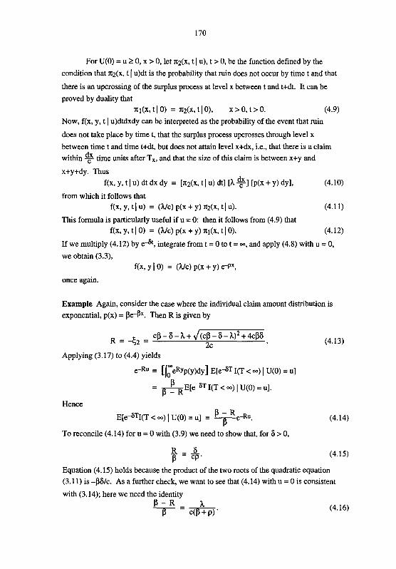
For U(0) = u 2 0, x > 0, let x2(x, t I u), t > 0, be the function defined by the

condition that K ~ ( x , t I u)dt is the probability that ruin does not occur by time t and that

there is an upcrossing of the surplus process at level x between t and t+dt. It can be

proved by duality that

xl(x, t I 0) = Q(x, t 1 o), X > 0, t > 0. (4.9) Now, f(x, y, t I u)dtdxdy can be interpreted as the probability of the event that ruin

does not take place by time t, that the surplus process upcrosses through level x

between time t and time t+dt, but does not attain level x+dx, i.e., that there is a claim within 9 time units after Tx, and that the size of this claim is between x+y and

x+y+dy. Thus

f(x, y, t 1 U) dt dx dy = [XZ(X, t I u) dtl [h 91 [p(x + y) dyl, (4.10)

from which it follows that

f(% y, t I U) = ( w p(x + y) x2(x, t 1 4. (4.1 1)

This formula is particularly useful if u = 0: then it follows from (4.9) that

f(x, y, t 1 0) = (hlc) p(x + y) RI(X, t 1 0). (4.12)

If we multiply (4.12) by eAt, integrate from t = 0 to t = m, and apply (4.8) with u = 0,

we obtain (3.3),

f(x, Y I 0) = (hlc) p(x + Y) d X 7

once again.

Example Again, consider the case where the individual claim amount distribution is exponential, p(x) = pe-px. Then R is given by

Applying (3.17) to (4.4) yields

e-Ru = [ / : e ~ ~ ~ ( ~ ) d ~ ] E[e4T I(T < m) I U(0) = u]

- - m ~ [ e A T P I(T < m) I U(0) = u].

Hence

E [ e A q ( ~ < 00) 1 U(0) = U] = i!j.Le-~". (4.14)

To reconcile (4.14) for u = 0 with (3.9) we need to show that, for 6 > 0,

R - 6 - v. (4.15)

Equation (4.15) holds because the product of the two roots of the quadratic equation (3.1 1) is -P6/c. As a further check, we want to see that (4.14) with u = 0 is consistent

with (3.14); here we need the identity P - R

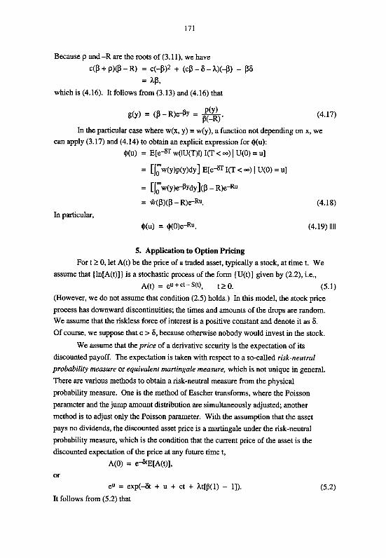
Because p and -R are the roots of (3.1 l), we have

c(P + P)@ - R) = c(-P)~ + ( 4 - 6 - U+) - P6

= LP, which is (4.16). It follows from (3.13) and (4.16) that

P(Y) g(y) = ($ - R)~-PY = - N-R) '

(4.17)

In the particular case where w(x, y) = w(y), a function not depending on x, we can apply (3.17) and (4.14) to obtain an explicit expression for $(u):

$(u) = E[ea w(lU(T)I) I(T < m) I U(0) = U]

In particular,

5. Application to Option Pricing For t 2 0, let A(t) be the price of a traded asset, typically a stock, at time t. We

assume that {ln[A(t)]J is a stochastic process of the form {U(t)) given by (2.2), i.e., A(t) = eu + ct - s(f), t 2 0. (5.1)

(However, we do not assume that condition (2.5) holds.) In this model, the stock price

process has downward discontinuities; the times and amounts of the drops are random. We assume that the riskless force of interest is a positive constant and denote it as 6.

Of course, we suppose that c > 6, because otherwise nobody would invest in the stock.

We assume that the price of a derivative security is the expectation of its

discounted payoff. The expectation is taken with respect to a so-called risk-neutral

probability measure or equivalent martingale measure, which is not unique in general.

There are various methods to obtain a risk-neutral measure from the physical

probability measure. One is the method of Esscher transforms, where the Poisson

parameter and the jump amount distribution are simultaneously adjusted; another

method is to adjust only the Poisson parameter. With the assumption that the asset

pays no dividends, the discounted asset price is a martingale under the risk-neutral

probability measure, which is the condition that the current price of the asset is the

discounted expectation of the price at any future time t,

A(0) = e 4 t ~ [ ~ ( t ) ] ,

or eU = exp(-6t + u + ct + ht[@(l) - I]).

It follows from (5.2) that

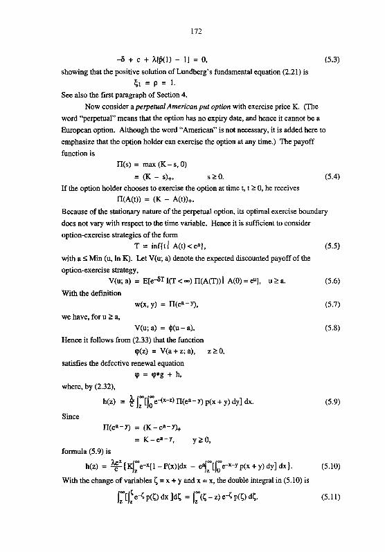
-6 + c + h@(l) - 11 = 0, (5.3) showing that the positive solution of Lundberg's fundamental equation (2.21) is

= p = 1.

See also the first paragraph of Section 4.

Now consider aperpetual American put option with exercise price K. (The

word "perpetual" means that the option has no expiry date, and hence it cannot be a

European option. Although the word "American" is not necessary, it is added here to

emphasize that the option holder can exercise the option at any time.) The payoff

function is n(s) = max (K - s, 0)

= (K - s)+, s 2 0. (5.4) If the option holder chooses to exercise the option at time t, t 2 0, he receives

n(A(t)) = (K - A(t))+. Because of the stationary nature of the perpetual option, its optimal exercise boundary

does not vary with respect to the time variable. Hence it is sufficient to consider

option-exercise strategies of the form T = inf(t 1 A(t) <ea], (5.5)

with a S Min (u, In K). Let V(u; a) denote the expected discounted payoff of the

option-exercise strategy, V(u; a) = ~ [ e a T I(T < m) lT(A(T)) 1 A(0) = eU], u 2 a.

With the definition W(X. y) = n(ea - Y),

we have, for u 2 a, V(u; a) = $(u - a).

Hence it follows from (2.33) that the function

q(z) = V(a + z; a), z 2 0,

satisfies the defective renewal equation

q = q*g + h,

where, by (2.32).

h(z) = $ /J;e+-z) n(ea- Y) p(x + y) dy] dr.

Since n(ea-Y) = (K-ea-Y),

= K-ea-Y, y 1 0 ,

formula (5.9) is

h(z) = ~ { ~ e - x [ l - P(x)]dx - ef;[\;e-~-y p(x + y) dy] dx}. (5.10)

With the change of variables = x + y and x = x, the double integral in (5.10) is

Because V(a; a) = cp(0) = h(O),

we can obtain an explicit expression for V(a; a). Applying (5.10). (5.11), and (2.38) [with 6 = p = 11, we have

V(a; a) = $ { K/;e-x[l- P(x)]dx - @I;< eei. ~ ( 4 ) dc )

= $[K(c - S)A + eaP(l)]. (5.12)

This result enables us to determine I , the optimal value of a (thus e q s the optimal

option-exercise stock price). If V(a; a) < n(ea),

we gather that I > a, and if

V(a; a) > n(ea),

we conclude that I < a. Hence I is determined by the continuous junction condition

V(I; I ) = lT(ea)

= K - ea. (5.13)

We substitute (5.12) with a = I in the left-hand side of (5.13) and obtain a linear

equation for eK .e solution is

ex = K 6

c + @'(I)'

Hence, for u 2 I , the price of the perpetual put option is V(u; I ) = Q(u - I). For u < I ,

the option is exercised immediately and its price is simply K - eU.

Remark It is intuitively clear that the optimal option-exercise stock price has to be less than the exercise price, i.e., ex < K. An algebraic proof that the fraction on the

right-hand side of (5.14) is between 0 and 1 goes as follows. Using (5.3) and the

inequality that

1 - e-Z > z e-Z, z > 0, we see that

0 < S = c - h[l - @(I)] DD

= c - h[l - lo ecZ p(z) dz]

DD

< c - hl,, z e-Z p(z) dz, (5.15)

which is the denominator on the right-hand side of (5.14). Hence the fraction in (5.14)

is indeed between 0 and 1.

Example Suppose that the jumps are exponentially distributed,

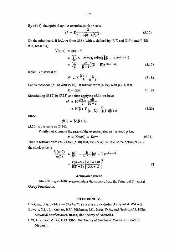
By (5.14), the optimal option-exercise stock price is

e h K 6

(5.16) c - h$(l + p)-2'

On the other hand, it follows from (5.8) [with w defined by (5.7) and (5.4)] and (4.18)

that, for u l a,

V(u; a) = $(u - a)

= [j;(~ - ea - Y)+ e-Pydy](P - R)e-R(~ - a)

= [f - &](a - R)~-R(U-~) , (5.17)

which is maximal at

e" K P + 1 R T R+1' (5.18)

Let us reconcile (5.18) with (5.16). It follows from (4.15), with p = 1, that

R = &PIC. (5.19)

Substituting (5.19) in (5.18) and then applying (5.3). we have

eH = K P + l 6P T s p + c

Since

P(1) = Pl(P + 1). (5.20) is the same as (5.16).

Finally, let K denote the ratio of the exercise price to the stock price,

k = WA(0) = Ke-a. (5.21)

Then it follows from (5.17) and (5.18) that, for u > 8, the ratio of the option price to

the stock price is

Acknowledgment Elias Shiu gratefully acknowledges the support from the Principal Financial

Group Foundation.

REFERENCES Beekman, J.A. 1974. Two Stochastic Processes. Stockholm: Almqvist & Wiksell.

Bowers, N.L., Jr., Gerber, H.U., Hickman, J.C., Jones, D.A., and Nesbitt, C.J. 1986.

Actuarial Mathematics. Itasca, Ill.: Society of Actuaries.

Cox, D.R., and Miller, H.D. 1965. The Theory of Stochastic Processes. London:

Methuen.

Dickson, D.C.M. 1992. "On the Distribution of Surplus prior to Ruin," Insurance:

Mathematics and Economics 11:191-207.

Dickson, D.C.M., and Egidio dos Reis, A.D. 1994. "Ruin Problems and Dual Events,"

Insurance: Mathematics and Economics 1451-60.

Dufresne, F., and Gerber, H.U. 1988. "The Surpluses Immediately before and at Ruin,

and the Amount of the Claim Causing Ruin," Insurance: Mathematics and

Economics 7: 193-199.

Gerber H.U. 1973. "Martingales in Risk Theory," Bulletin of the Swiss Association of

Actuaries, 205-216.

Gerber, H.U. 1990. "When Does the Surplus Reach a Given Target?" Insurance:

Mathematics and Economics 9: 115-1 19.

Gerber H.U., and Shiu, E.S.W. 1994a. "Option Pricing by Esscher Transforms,"

Transactions, Sociefy of Actuaries XLVI:99-140; Discussion 141-191.

Gerber H.U., and Shiu, E.S.W. 199413. "Martingale Approach to Pricing Perpetual

American Options," ASTIN Bulletin 24:195-220.

Gerber H.U., and Shiu, E.S.W. 1996a. "Martingale Approach to Pricing Perpetual

American Options on TWO Stocks," Mathematical Finance 6:303-322.

Gerber H.U., and Shiu, E.S.W. 1996b. "Actuarial Bridges to Dynamic Hedging and

Option Pricing," Insurance: Mathematics and Economics 18:183-218.

Gerber H.U., and Shiu, E.S.W. 1997. "On the Time Value of Ruin," Actuarial

Research Clearing House 1997.1, 145-199. A revised version will appear in

Volume 2 (1998) of the North American Actuarial Journal.

Kendall, D.G. 1957. "Some Problems in the Theory of Dams," Journal of the Royal

Statistical Society Series B 19:207-212.

Lundberg, F. 1932. "Some Supplementary Researches on the Collective Risk Theory,"

Skandinavisk Aktuarietidskrifr 15: 137-158.

Michaud, F. 1996. Essays on Option Pricing with Jump Processes and an Estimation

Technique in Ruin Theory. Doctoral Thesis, University of Lausanne.

Michaud, F. 1997. "Shifted Poisson Processes and the Pricing of Perpetual American

Options," submitted for publication.

Panjer, H.H., and Willmot, G.E. 1992. Insurance Risk Models. Schaumburg, Ill.:

Society of Actuaries.

Prabhu, N.U. 1961. "On the Ruin Problem of Collective Risk Theory," Annals of

Mathematical Statistics 32:757-764.

Prabhu, N.U. 1980. Stochastic Storage Processes: Queues, Insurance Risk, and Dams.

New York: Springer-Verlag.

Seal, H.L. 1969. Stochastic Theory of a Risk Business. New York: Wiley.

Takhcs, L. 1967. Cornbinatorial Methods in the Theory of Stochastic Processes. New

York: Wiley. Reprinted by Krieger, Huntington, N.Y., 1977.