From Prices to Business Cycles - FGV...
83
From Prices to Business Cycles Joªo V. Issler (FGV) and Claudia Rodrigues (VALE) May, 2013 J.V. Issler, C.F. Rodrigues Prices and Business Cycles May, 2013 1/2
Transcript of From Prices to Business Cycles - FGV...

From Prices to Business Cycles
João V. Issler (FGV) and Claudia Rodrigues (VALE)
May, 2013
J.V. Issler, C.F. Rodrigues () Prices and Business Cycles May, 2013 1 / 2

Outline
Two talks for the price of one :-))
Our theme in both talks is: �from prices to business cycles.�
First paper covers asset prices and consumption business cycles(intertemporal substitution).
We exploit theoretical commonality among prices to identifyprice-quantity relationships.
Second paper covers metal-commodity prices and cycles in GlobalIndustrial Production (and Global GDP).
We exploit short-run restrictions in the equilibrium condition for inputmarkets to identify price-quantity relationships.
In both papers we employ common-feature techniques in estimationand testing.
We illustrate the usefulness of our results in empirical exercises.
J.V. Issler, C.F. Rodrigues () Prices and Business Cycles May, 2013 2 / 2

A Stochastic Discount Factor Approach to Asset Pricingusing Panel Data Asymptotics
Fabio Araujo (Central Bank of Brazil) and João Victor Issler (FGV)
May, 2013
F. Araujo and J.V. Issler ()VALE/EPGE: Panel-Data SDF Approach May, 2013 1 / 37

Motivation �Why Consumption Cycles?
Research is done mostly using GDP/GNP cycles. But:
.05
.04
.03
.02
.01
.00
.01
.02
.03
.04
55 60 65 70 75 80 85 90 95 00 05 10
HP CYCLE GDP USAHP CYCLE CONS REAL
Synchronized cycles for HP �ltered consumption and GDP. Similarpicture for Beveridge-Nelson cycles; Issler and Vahid (JME, 2001).
F. Araujo and J.V. Issler ()VALE/EPGE: Panel-Data SDF Approach May, 2013 2 / 37

This Paper
We impose no-arbitrage to show that the SDF is a common featureof all asset returns.
Our estimator is based on the Asset-Pricing Equation: it is a novelconsistent estimator of the SDF based on return (price) data alone;Harrison and Kreps (1979), Hansen and Richard (1987), and Hansenand Jagannathan (1991, 1997).
This allows consistent estimation of the stochastic process of the SDFfMtg∞
t=1 without resorting to any parametric assumptions onpreferences.
This also allows the development of no-arbitrage estimators of theSDF and of asset-return volatility and conditional volatility. Theycould be used as theory-based estimators (quasi-structural) to becompared to unrestricted reduced-form estimators.
F. Araujo and J.V. Issler ()VALE/EPGE: Panel-Data SDF Approach May, 2013 3 / 37

This Paper
We bridge the gap between a large literature on common features inmacro [Vahid and Engle (1993, 1997), Engle and Issler (1995), Isslerand Vahid (2001, 2006), Hecq, Palm and Urbain (2006), Issler andLima (2009), and Athanasopoulos et al. (2011)] and the �nanceliterature using common components in mean and variance[Aït-Sahalia and Lo (1998, 2000), Lettau and Ludvigson (2001),Rosenberg and Engle (2002), Garcia, Renault, and Semenov (2006),Sentana and Peñaranda (2008), Hansen and Scheinkman (2009), andHansen and Renault (2009), Peñaranda and Sentana (2010)].We also propose an alternative way of imposing no-arbitrage inconstructing important �nancial econometrics estimators, whichbecame popular through the work of Diebold and Li (2006),Christensen, Diebold, and Rudebusch (2007, 2009, 2011), andDiebold and Rudebusch (2013).The estimation technique is based on standard panel-dataasymptotics.
F. Araujo and J.V. Issler ()VALE/EPGE: Panel-Data SDF Approach May, 2013 4 / 37

Assumptions
Assumption 1: We assume the absence of arbitrage opportunities in assetpricing, c.f., Ross (1976). This must hold for allt = 1, 2, ...,T , and for all lapses of time, however small.
Basically, Assumption 1 is a necessary and su¢ cient condition for (1)to hold; Cochrane (2002). In Hansen and Renault (2009), it implies(1):
pi ,t = Et
�βU 0 (ct+1)U 0 (ct )
(pi ,t+1 + di ,t+1)�, 8i
1 = Et
�βU 0 (ct+1)U 0 (ct )
xi ,t+1pi ,t
�, i = 1, 2, ...,N
1 = Et fMt+1Ri ,t+1g , i = 1, 2, ...,N. (1)
F. Araujo and J.V. Issler ()VALE/EPGE: Panel-Data SDF Approach May, 2013 5 / 37

Assumptions
The absence of arbitrage opportunities has two important implications:
1 There exists at least one stochastic discount factor Mt , for whichMt > 0 for all t. This is due to the fact that, when we consider theexistence derivatives on traded assets, arbitrage opportunities willarise if Mt � 0; Hansen and Jagannathan (1997).
2 A weak law-of-large numbers (WLLN) holds in the cross-sectionaldimension for the level of gross returns Ri ,t ; Ross (1976).
The Pricing Equation (1) is present in virtually all studies dealing withintertemporal substitution; e.g., Hansen and Singleton (1982, 1983, 1984),Mehra and Prescott (1985), Epstein and Zin (1991), Fama and French(1992, 1993), Attanasio and Browning (1995), Lettau and Ludvigson(2001), Garcia, Renault, and Semenov (2006), and Hansen andScheinkman (2009).
F. Araujo and J.V. Issler ()VALE/EPGE: Panel-Data SDF Approach May, 2013 6 / 37

Assumptions
Assumption 2: Let Rt = (R1,t ,R2,t , ... RN ,t )0 be an N � 1 vector
stacking all asset returns in the economy and consider thevector process
nln (MtR0t )
0o. In the time (t) dimension, we
assume thatnln (MtR0t )
0o∞
t=1is covariance-stationary and
ergodic with �nite �rst and second moments uniformlyacross i .
Weak stationarity of returns can coexist with conditionalheteroskedasticity; see Engle (1982) and Bollerslev (1986). This �tswell established properties of asset returns.
F. Araujo and J.V. Issler ()VALE/EPGE: Panel-Data SDF Approach May, 2013 7 / 37

Exact Taylor Expansion
Consider a second-order Taylor Expansion of the exponential functionaround x , with increment h, as follows:
ex+h = ex + hex +h2ex+λ(h)�h
2, (2)
with λ(h) : R ! (0, 1) . (3)
For the expansion of a generic function, λ(�) would depend on x and h.However, dividing (2) by ex :
eh = 1+ h+h2eλ(h)�h
2, (4)
shows that (4) does not depend on x .
F. Araujo and J.V. Issler ()VALE/EPGE: Panel-Data SDF Approach May, 2013 8 / 37
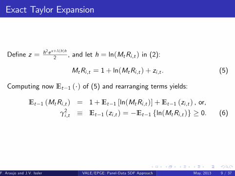
Exact Taylor Expansion
De�ne z = h2ex+λ(h)h
2 , and let h = ln(MtRi ,t ) in (2):
MtRi ,t = 1+ ln(MtRi ,t ) + zi ,t . (5)
Computing now Et�1 (�) of (5) and rearranging terms yields:
Et�1 (MtRi ,t ) = 1+Et�1 [ln(MtRi ,t )] +Et�1 (zi ,t ) , or,
γ2i ,t � Et�1 (zi ,t ) = �Et�1 fln(MtRi ,t )g � 0. (6)
F. Araujo and J.V. Issler ()VALE/EPGE: Panel-Data SDF Approach May, 2013 9 / 37

Quasi-Structural Factor Model (in logs)
Let γ2t ��γ21,t γ22,t ... γ2N ,t
�0 and εt � (ε1,t ε2,t ... εN ,t )0:
ln(MtRt ) = Et�1fln(MtRt )g+ εt
= �γ2t + εt .
Denoting by rt = ln (Rt ) and by mt = ln (Mt ):
ri ,t = �mt � γ2i ,t + εi ,t , i = 1, 2, . . . ,N. (7)
mt is a common feature of all (logged) asset returns; Engle andKozicki (1993). Also, Hansen and Singleton (JPE, 1983).
εi ,t = ln(MtRi ,t )�Et�1fln(MtRi ,t )g =(mt + ri ,t )�Et�1 (mt + ri ,t ) is the innovation on mt + ri ,t .
F. Araujo and J.V. Issler ()VALE/EPGE: Panel-Data SDF Approach May, 2013 10 / 37

Quasi-Structural Factor Model (in logs)
Wold representation from Assumption 2:
ln(MtRi ,t ) = µi +∞
∑j=0bi ,j εi ,t�j (8)
where, for all i , bi ,0 = 1, jµi j < ∞, ∑j b2i ,j < ∞, and εi ,t is white noise.
Now:γ2i ,t � Et�1 (zi ,t ) = �Et�1 fln(MtRi ,t )g
Then:
ri ,t = �mt � γ2i + εi ,t +∞
∑j=1bi ,j εi ,t�j , i = 1, 2, . . . ,N, (9)
where γ2i � �µi .
F. Araujo and J.V. Issler ()VALE/EPGE: Panel-Data SDF Approach May, 2013 11 / 37

Quasi-Structural Factor Model (in logs)
Special case: assume ln(MtRt )j It�1 � N [Et�1 (rt + ιmt ) ,Σ], i.e., MtRthas a multivariate log-Normal homoskedastic distribution. Then,
Et�1 (MtRi ,t ) = exp�
Et�1 (ri ,t +mt ) +σ2i2
�= 1, or,
Et�1 (ri ,t +mt ) +σ2i2
= 0, or, using
ri ,t +mt = Et�1 (ri ,t +mt ) + εi ,t , yields,
ri ,t = �mt �σ2i2+ εi ,t i = 1, 2, . . . ,N. (10)
F. Araujo and J.V. Issler ()VALE/EPGE: Panel-Data SDF Approach May, 2013 12 / 37

Law-of-Large Numbers for (11)
Consider now a cross-sectional average of (9):
1N
N
∑i=1ri ,t = �mt �
1N
N
∑i=1
γ2i +1N
N
∑i=1
εi ,t +1N
N
∑i=1
∞
∑j=1bi ,j εi ,t�j . (11)
The stochastic terms in the cross-sectional dimension have the followingvariance:
VAR
1N
N
∑i=1
εi ,t
!+VAR
1N
N
∑i=1bi ,1εi ,t�1
!+VAR
1N
N
∑i=1bi ,2εi ,t�2
!+ � � �
since there is no time-series correlation in εt � (ε1,t ε2,t ... εN ,t )0 due to
assumption of weak stationarity.
F. Araujo and J.V. Issler ()VALE/EPGE: Panel-Data SDF Approach May, 2013 13 / 37

Skepticism on Law-of-Large Numbers for (11)
We can always decompose εi ,t as:
εi ,t = ln(MtRi ,t )�Et�1fln(MtRi ,t )g= [mt �Et�1 (mt )] + [ri ,t �Et�1 (ri ,t )]
= qt + vi ,t = αi|{z}1+
COV(vi ,t ,qt )VAR(qt )
=1+δi
qt + ξ i ,t
plimN!∞
1N
N
∑i=1
εi ,t = 0 =) limN!∞
1N
N
∑i=1
δi = �1.
This an identi�cation issue.Alternative (Ergodic Theorem): no-arbitrage requires 1
N ∑Ni=1 Ri ,t
p!,implying 1
N ∑Ni=1 ri ,t
p!Here: with quasi-structural system no-arbitrage impliesplimN!∞
1N ∑N
i=1 εi ,t = 0.
F. Araujo and J.V. Issler ()VALE/EPGE: Panel-Data SDF Approach May, 2013 14 / 37

Main Result
TheoremUnder Assumptions 1 and 2, as N,T ! ∞, with N diverging at a rate atleast as large as T , the realization of the SDF at time t, denoted by Mt ,can be consistently estimated using:
bMt =RGt
1T
T∑j=1
�RGj R
Aj
� ,
where RGt = ∏N
i=1 R� 1N
i ,t and RAt =
1N
N∑i=1Ri ,t are respectively the
geometric average of the reciprocal of all asset returns and the arithmeticaverage of all asset returns.
F. Araujo and J.V. Issler ()VALE/EPGE: Panel-Data SDF Approach May, 2013 15 / 37

Sketch of the Proof
Stacked quasi-structural form imposing with Log-Normality:[email protected]
1CCCA = �mt
1CCCA�0BBB@
σ21σ22...
σ2N
1CCCA+0BBB@
ε1tε2t...
εNt
1CCCA .An arbitrage portfolio with weights wi , all of order N�1 in absolute value,stacked in a vector WN = (w1,w2, ...,wN )
0, obeys:
W 0N
1CCCA = 0, limN!∞
W 0N
1CCCA = 0, limN!∞
VAR
26664W 0N
0BBB@r1,tr2,t...rN ,t
1CCCA37775 = 0.(12)
F. Araujo and J.V. Issler ()VALE/EPGE: Panel-Data SDF Approach May, 2013 16 / 37

Sketch of the Proof
No-arbitrage imposes restrictions on the limit return of arbitrage portfolios:
plimN!∞
W 0N
0BBB@r1,tr2,t...rN ,t
1CCCA = 0. (13)
A weak inequality (� 0) does not work, because portfolio �W 0N would still
be an arbitrage portfolio, it obeys (12), and it would violate (13).
F. Araujo and J.V. Issler ()VALE/EPGE: Panel-Data SDF Approach May, 2013 17 / 37

Sketch of the Proof
No arbitrage (13) requires:
0 = �mt limN!∞
W 0N
0B@ 1...1
1CA� limN!∞
W 0N
0BB@σ212...
σ2N2
1CCA+ plimN!∞
W 0N
0B@ ε1,t...
εN ,t
1CA
= � limN!∞
W 0N
0BB@σ212...
σ2N2
1CCA+ plimN!∞
W 0N
2640B@ 1...1
1CA+0B@ δ1
...δN
1CA375 qt
+plimN!∞
W 0N
0B@ ξ1,t...
ξN ,t
1CA .
F. Araujo and J.V. Issler ()VALE/EPGE: Panel-Data SDF Approach May, 2013 18 / 37

Sketch of the Proof
W 0N must lie in the left-null space of
0B@ 1...1
1CA, to preventplimN!∞
W 0N
0B@ r1,t...rN ,t
1CA to depend on qt :
0B@ δ1...
δN
1CA =
0B@ δ...δ
1CA , jδj < ∞,
Otherwise, for some realizations of qt we could not prevent that
plimN!∞
W 0N
0B@ r1,t...rN ,t
1CA > 0, or plimN!∞
W 0N
0B@ r1,t...rN ,t
1CA < 0, which violate no
arbitrage.F. Araujo and J.V. Issler ()VALE/EPGE: Panel-Data SDF Approach May, 2013 19 / 37
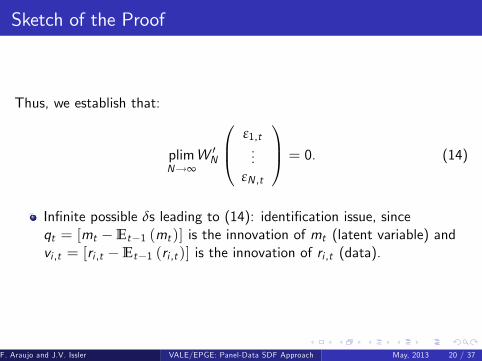
Sketch of the Proof
Thus, we establish that:
plimN!∞
W 0N
0B@ ε1,t...
εN ,t
1CA = 0. (14)
In�nite possible δs leading to (14): identi�cation issue, sinceqt = [mt �Et�1 (mt )] is the innovation of mt (latent variable) andvi ,t = [ri ,t �Et�1 (ri ,t )] is the innovation of ri ,t (data).
F. Araujo and J.V. Issler ()VALE/EPGE: Panel-Data SDF Approach May, 2013 20 / 37

Sketch of the Proof � Identi�cation of SDF
Identi�cation of qt and thus of mt , requires a choice of δ.
plimN!∞
1N
N
∑i=1
εi ,t = (1+ δ) qt . (15)
Identi�cation of qt and thus of mt , requires a choice of δ. The choiceδ = �1, for all i , yields plim
N!∞
1N ∑N
i=1 εi ,t = 0.
The choice δ = �1, for all i , makes εi ,t uncorrelated with qt for all i .
F. Araujo and J.V. Issler ()VALE/EPGE: Panel-Data SDF Approach May, 2013 21 / 37

Sketch of the Proof �Meaning of Identi�cationAssumption
Take (10), average across i and take the probability limit to obtain:
plimN!∞
1N
N
∑i=1ri ,t = �mt �
12
limN!∞
1N
N
∑i=1
σ2i
!+ plimN!∞
1N
N
∑i=1
εi ,t
= �mt �12
limN!∞
1N
N
∑i=1
σ2i
!,
which yields:
VAR
plimN!∞
1N
N
∑i=1ri ,t
!= VAR (mt ) , (16)
where VAR(�) is computed in the time-series dimension.
F. Araujo and J.V. Issler ()VALE/EPGE: Panel-Data SDF Approach May, 2013 22 / 37

Sketch of the Proof
We have:
1N
N
∑i=1ri ,t = �mt �
121N
N
∑i=1
σ2i +1N
N
∑i=1
εi ,t . (17)
Take the probability limit as N ! ∞:
1N
N
∑i=1e(�
12 σ2i ) ! eγ2 , say.
Using Slutsky�s Theorem, we can then propose a consistent estimatorfor a tilted version of Mt (eγ2 �Mt = eMt):
beM t =N
∏i=1R� 1N
i ,t . (18)
F. Araujo and J.V. Issler ()VALE/EPGE: Panel-Data SDF Approach May, 2013 23 / 37

Sketch of the Proof
Multiply the Pricing Equation for every asset by e(�12 σ2i ) to get:
e(�12 σ2i ) = Et�1
ne(�
12 σ2i )MtRi ,t
o= Et�1
n eMtRi ,to.
Take now the unconditional expectation, use the law-of-iteratedexpectations, and average across i = 1, 2, ...,N to get, for large enough N:
eγ2 =1N
N
∑i=1
En eMtRi ,t
o.
F. Araujo and J.V. Issler ()VALE/EPGE: Panel-Data SDF Approach May, 2013 24 / 37

Sketch of the Proof
Thus, for large enough N, it is straightforward to obtain a consistentestimator for eγ2 = lim
N!∞1N ∑N
i=1 e(� 1
2 σ2i ) using (18):
ceγ2 =1N
N
∑i=1
1T
T
∑t=1
beM tRi ,t
!=1T
T
∑t=1
N
∏i=1R� 1N
i ,t1N
N
∑i=1Ri ,t
!(19)
=1T
T
∑t=1RGt R
At , (20)
where, in this last step, N must diverge at a rate at least as fast as T ,
otherwise we would not be able to exchange eMt bybeM t in (19).
F. Araujo and J.V. Issler ()VALE/EPGE: Panel-Data SDF Approach May, 2013 25 / 37

Sketch of the Proof
Then, a consistent estimator for Mt is:
bMt =beM tceγ2=
RGt
1T ∑T
τ=1 RGτ R
Aτ
.
F. Araujo and J.V. Issler ()VALE/EPGE: Panel-Data SDF Approach May, 2013 26 / 37

Remarks
Hansen and Jagannathan (1991):
M�t+1 = ι0
�Et�Rt+1R 0t+1
���1 Rt+1, or,M�t+1 = ι0
�E�Rt+1R 0t+1
���1 Rt+1,Theoretical problems for Et
�Rt+1R 0t+1
�and E
�Rt+1R 0t+1
�which are
of in�nite order when N ! ∞. Theoretical problems inverting themwhen N ! ∞ faster than T ! ∞.Need a model to compute Et
�Rt+1R 0t+1
�.
Numerical problems inverting Et�Rt+1R 0t+1
�and E
�Rt+1R 0t+1
�for
large N.
F. Araujo and J.V. Issler ()VALE/EPGE: Panel-Data SDF Approach May, 2013 27 / 37

Remarks
Identi�cation:
bMtp�! Mt = M�
t > 0, unique SDF, if markets are complete,
In complete markets we identify the unique SDF which is equal to themimicking portfolio.
bMtp�! Mt > 0, SDF>0, if markets are incomplete.
In incomplete markets we can only identify SDFs up to addition of anerror term, irrelevant for pricing assets. Our estimator identi�espositive SDFs or combinations of them. They all have identicalpricing properties.
F. Araujo and J.V. Issler ()VALE/EPGE: Panel-Data SDF Approach May, 2013 28 / 37

Testing Preference Speci�cations
Popular Preference representations:
CRRA Mt+1 = β�ct+1ct
��γ
ExternalHabit
Mt+1 = β�ctct�1
�κ(γ�1) �γct+1ct
��γ
Kreps-Porteus Mt+1 =
�β�ct+1ct
��γ� α
ρ h1
Bt+1
i1� αρ
F. Araujo and J.V. Issler ()VALE/EPGE: Panel-Data SDF Approach May, 2013 29 / 37

Testing Preference Speci�cations
Our sample period starts in 1972:1 and ends in 2000:4 in quarterlyfrequency.
We averaged the real U.S.$ returns on 18 portfolios or individualassets, taking into account the returns or more than thousands ofassets.
Real returns were computed using the consumer price index in theU.S. Our database covers U.S.$ real returns on G7-country stockindices and short-term government bonds. In addition, we also useU.S.$ real returns on Gold, real estate, bonds on AAA U.S.corporations, and on the SP 500. The U.S. government bond ischosen to be the 90-day T-Bill.
Consumption data and income data: seasonally adjusted real totalprivate consumption and GNP per-capita.
F. Araujo and J.V. Issler ()VALE/EPGE: Panel-Data SDF Approach May, 2013 30 / 37

Testing Preference Speci�cations
The sample mean of cMt is 0.9927, implying an annual discount factor of0.9711, or an annual discount rate of 2.97%.
0.85
0.90
0.95
1.00
1.05
1.10
1.15
1975 1980 1985 1990 1995 2000
F. Araujo and J.V. Issler ()VALE/EPGE: Panel-Data SDF Approach May, 2013 31 / 37
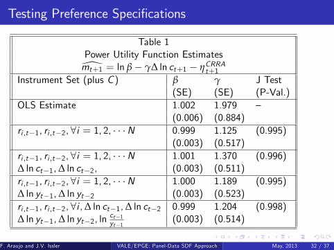
Testing Preference Speci�cations
Table 1Power Utility Function Estimates[mt+1 = ln β� γ∆ ln ct+1 � ηCRRAt+1
Instrument Set (plus C ) β γ J Test(SE) (SE) (P-Val.)
OLS Estimate 1.002 1.979 �(0.006) (0.884)
ri ,t�1, ri ,t�2, 8i = 1, 2, � � �N 0.999 1.125 (0.995)(0.003) (0.517)
ri ,t�1, ri ,t�2, 8i = 1, 2, � � �N 1.001 1.370 (0.996)∆ ln ct�1,∆ ln ct�2, (0.003) (0.511)ri ,t�1, ri ,t�2, 8i = 1, 2, � � �N 1.000 1.189 (0.995)∆ ln yt�1,∆ ln yt�2 (0.003) (0.523)ri ,t�1, ri ,t�2, 8i ,∆ ln ct�1,∆ ln ct�2 0.999 1.204 (0.998)∆ ln yt�1,∆ ln yt�2, ln
ct�1yt�1
(0.003) (0.514)
F. Araujo and J.V. Issler ()VALE/EPGE: Panel-Data SDF Approach May, 2013 32 / 37

Testing Preference Speci�cations
Table 2External Habit Utility Function Estimates
[mt+1 = ln β� γ∆ ln ct+1 + κ (γ� 1)∆ ln ct � ηEHt+1Instrument Set (plus C ) β γ κ J-Test
(SE) (SE) (SE) (P-Val)OLS Estimate 1.002 1.975 -0.008 �
(0.006) (0.97) (0.99)ri ,t�1, ri ,t�2, 8i = 1, 2, � � �N 1.005 1.263 -2.847 (0.991)
(0.003) (0.61) (8.33)ri ,t�1, ri ,t�2, 8i = 1, 2, � � �N, 0.9954 1.308 1.997 (0.995)∆ ln ct�1,∆ ln ct�2 (0.003) (0.56) (3.27)ri ,t�1, ri ,t�2, 8i = 1, 2, � � �N, 0.987 1.592 3.588 (0.995)∆ ln yt�1,∆ ln yt�2 (0.003) (0.68) (3.74)ri ,t�1, ri ,t�2, 8i ,∆ ln ct�1,∆ ln ct�2 0.987 1.161 8.834 (0.998)∆ ln yt�1,∆ ln yt�2, ln
ct�1yt�1
(0.002) (0.62) (32.76)
F. Araujo and J.V. Issler ()VALE/EPGE: Panel-Data SDF Approach May, 2013 33 / 37

Testing Preference Speci�cations
Table 3Kreps�Porteus Utility Function Estimates
[mt+1 = θ ln β� θγ∆ ln ct+1 � (1� θ) lnBt+1 � ηKPt+1Instrument Set (plus C ) β γ θ J-Test
(SE) (SE) (SE) (P-Val.)OLS Estimate 1.007 3.141 0.831 �
(0.006) (0.88) (0.02)ri ,t�1, ri ,t�2, 8i = 1, 2, � � �N 1.001 1.343 0.933 (0.996)
(0.004) (0.72) (0.01)ri ,t�1, ri ,t�2, 8i = 1, 2, � � �N, 1.003 1.360 0.922 (0.998)∆ ln ct�1,∆ ln ct�2 (0.004) (0.76) (0.01)ri ,t�1, ri ,t�2, 8i = 1, 2, � � �N, 1.000 0.926 0.927 (0.996)∆ ln yt�1,∆ ln yt�2 (0.004) (0.75) (0.01)ri ,t�1, ri ,t�2, 8i ,∆ ln ct�1,∆ ln ct�2 0.997 0.362 0.901 (0.999)∆ ln yt�1,∆ ln yt�2, ln
ct�1yt�1
(0.004) (0.76) (0.01)
F. Araujo and J.V. Issler ()VALE/EPGE: Panel-Data SDF Approach May, 2013 34 / 37

Testing Preference Speci�cations �Consumption FactorAlone
3
2
1
0
1
2
3
4
.020
.015
.010
.005
.000
.005
.010
.015
72 74 76 78 80 82 84 86 88 90 92 94 96 98 00
Cons. Growth (X1)SDF Estimate
ρ = 0.21
F. Araujo and J.V. Issler ()VALE/EPGE: Panel-Data SDF Approach May, 2013 35 / 37

Testing Preference Speci�cations - Two-FactorKreps-Porteus Model
4
3
2
1
0
1
2
3
4
72 74 76 78 80 82 84 86 88 90 92 94 96 98 00
SDF KP Model (scaled)SDF Estimate (scaled)
ρ = 0.61
F. Araujo and J.V. Issler ()VALE/EPGE: Panel-Data SDF Approach May, 2013 36 / 37

Conclusions and Further Results
1 Assuming no arbitrage, and that the we can consistently estimate the�rst two moments of asset-return and SDF data, we can use assetreturn (price) data to model intertemporal substitution withoutspecifying preferences.
2 All our estimators can be labelled no-arbitrage estimators.3 We generate a template to evaluate preferences and intertemporalsubstitution models (similarly to Hansen and Jagannathan, 1991,1997).
4 Our results could be use a mixed-frequency to model and predictconsumption cycles, as well as GDP cycles, as long as we can tie upthese two together in a structural-equation setup.
F. Araujo and J.V. Issler ()VALE/EPGE: Panel-Data SDF Approach May, 2013 37 / 37
Common Features for Metal-Commodity Prices andGlobal Business Cycles
João V. Issler (FGV), Claudia Rodrigues (VALE), Rafael Burjack (FGV)
May, 2013
J.V. Issler, C.F. Rodrigues, and R. Burjack ()Metal Prices and Business Cycles May, 2013 1 / 29

Global GDP and IP growth rates
6
5
4
3
2
1
0
1
2
3
92 94 96 98 00 02 04 06 08 10
GDP Growth Rates (std)Ind. Prod. Growth Rates (std)
J.V. Issler, C.F. Rodrigues, and R. Burjack ()Metal Prices and Business Cycles May, 2013 2 / 29

Copper prices and global IP growth
5
4
3
2
1
0
1
2
3
92 94 96 98 00 02 04 06 08 10
Copper Prices Growth Rates (std)Global Ind. Prod. Growth Rates (std)
Sources: LME and J.P.Morgan
J.V. Issler, C.F. Rodrigues, and R. Burjack ()Metal Prices and Business Cycles May, 2013 3 / 29

Outline of the Talk
1 Basic concepts: Features and Common Features
2 Econometric models that incorporate common features3 Common Cycles between Metal Prices and Industrial Production4 Forecastability performance of econometric models with and withoutMetal-Price Information to predict GDP
J.V. Issler, C.F. Rodrigues, and R. Burjack ()Metal Prices and Business Cycles May, 2013 4 / 29

Outline of the Talk
1 Basic concepts: Features and Common Features2 Econometric models that incorporate common features
3 Common Cycles between Metal Prices and Industrial Production4 Forecastability performance of econometric models with and withoutMetal-Price Information to predict GDP
J.V. Issler, C.F. Rodrigues, and R. Burjack ()Metal Prices and Business Cycles May, 2013 4 / 29

Outline of the Talk
1 Basic concepts: Features and Common Features2 Econometric models that incorporate common features3 Common Cycles between Metal Prices and Industrial Production
4 Forecastability performance of econometric models with and withoutMetal-Price Information to predict GDP
J.V. Issler, C.F. Rodrigues, and R. Burjack ()Metal Prices and Business Cycles May, 2013 4 / 29

Outline of the Talk
1 Basic concepts: Features and Common Features2 Econometric models that incorporate common features3 Common Cycles between Metal Prices and Industrial Production4 Forecastability performance of econometric models with and withoutMetal-Price Information to predict GDP
J.V. Issler, C.F. Rodrigues, and R. Burjack ()Metal Prices and Business Cycles May, 2013 4 / 29

Common Features �Basic Ideas
1 Series y1t has property A.
2 Series y2t has property A.3 There exists a linear combination of them, y1t � eαy2t , that does nothave property A.
4 Cointegration is the most well-known example of common features.5 Serial correlation-common features (SCCF) or common cycles are alsowell-known: stationary series y1t and y2t both have serial correlation(are predictable), but there exists y1t � eαy2t which is white noise(unpredictable).
J.V. Issler, C.F. Rodrigues, and R. Burjack ()Metal Prices and Business Cycles May, 2013 5 / 29

Common Features �Basic Ideas
1 Series y1t has property A.2 Series y2t has property A.
3 There exists a linear combination of them, y1t � eαy2t , that does nothave property A.
4 Cointegration is the most well-known example of common features.5 Serial correlation-common features (SCCF) or common cycles are alsowell-known: stationary series y1t and y2t both have serial correlation(are predictable), but there exists y1t � eαy2t which is white noise(unpredictable).
J.V. Issler, C.F. Rodrigues, and R. Burjack ()Metal Prices and Business Cycles May, 2013 5 / 29

Common Features �Basic Ideas
1 Series y1t has property A.2 Series y2t has property A.3 There exists a linear combination of them, y1t � eαy2t , that does nothave property A.
4 Cointegration is the most well-known example of common features.
5 Serial correlation-common features (SCCF) or common cycles are alsowell-known: stationary series y1t and y2t both have serial correlation(are predictable), but there exists y1t � eαy2t which is white noise(unpredictable).
J.V. Issler, C.F. Rodrigues, and R. Burjack ()Metal Prices and Business Cycles May, 2013 5 / 29

Common Features �Basic Ideas
1 Series y1t has property A.2 Series y2t has property A.3 There exists a linear combination of them, y1t � eαy2t , that does nothave property A.
4 Cointegration is the most well-known example of common features.5 Serial correlation-common features (SCCF) or common cycles are alsowell-known: stationary series y1t and y2t both have serial correlation(are predictable), but there exists y1t � eαy2t which is white noise(unpredictable).
J.V. Issler, C.F. Rodrigues, and R. Burjack ()Metal Prices and Business Cycles May, 2013 5 / 29

Common cycle
J.V. Issler, C.F. Rodrigues, and R. Burjack ()Metal Prices and Business Cycles May, 2013 6 / 29

Common cycles
J.V. Issler, C.F. Rodrigues, and R. Burjack ()Metal Prices and Business Cycles May, 2013 7 / 29

Common Features �Basic Ideas
1 Engle and Kozicki (1993) main example: No cointegration forlog-levels of GDP for the U.S. and Canada. Instantaneous growthrates of GDP for the U.S. and Canada have serial correlation andthere is a linear combination of growth rates that is white noise.Cycles in U.S. and Canadian GDP growth are synchronized.
2 Our main �nding: common serial correlation between growth rates ofindustrial production and metal commodity prices (e.g., Copper):�
∆ lnPCOPPERt∆ ln IPt
�=
�λ1
�ft +
�εCOPPERt
εIPt
�, or,
∆ lnPCOPPERt � λ∆ ln IPt = εCOPPERt � λεIPt ,�1 �λ
�is the cofeature vector, eliminating the SCCF.
J.V. Issler, C.F. Rodrigues, and R. Burjack ()Metal Prices and Business Cycles May, 2013 8 / 29

Common Features �Useful Dynamic Representations
Vahid and Engle (1993): VAR for yt , an n-vector of I (1) variables:
yt = Γ1yt�1 + . . .+ Γpyt�p + εt . (1)
VECM:
∆ yt = Γ�1 ∆ yt�1 + . . . + Γ�p�1 ∆ yt�p+1 + γα0 yt�1 + εt . (2)
Normalized cofeature vectors:
α̃ =
�Is
α̃�(n�s)�s
�Quasi-structural model (restricted VECM):
"Is α̃�0
0(n�s)�s
In�s
#∆ yt =
"0
s�(np+r )Γ��1 . . . Γ��p�1 γ�
# 26664∆ yt�1...
∆ yt�p+1α0yt�1
37775+ vt . (3)J.V. Issler, C.F. Rodrigues, and R. Burjack ()Metal Prices and Business Cycles May, 2013 9 / 29

Common Cycles not considered in the model
VECM:8>>>>>>>>>>>>>><>>>>>>>>>>>>>>:
∆ y1t= Γ�11 ∆ y1t�1+Γ�12 ∆ y2t�1+ . . .+ Γ�1n ∆ ynt�1+...+Γ�p�1,1 ∆ y1,t�p+1+ . . .+ Γ�p�1,n ∆ yn,t�(p�1)+γα0 y t�1+ε1t......
∆ ynt= Φ�11 ∆ y1t�1+Φ�
12 ∆ y2t�1+ . . .+Φ�1n ∆ ynt�1+...
+Φ�p�1,1 ∆ y1,t�p+1+ . . .+Φ�
p�1,n ∆ yn,t�(p�1)+ηα0 y t�1+εnt
J.V. Issler, C.F. Rodrigues, and R. Burjack ()Metal Prices and Business Cycles May, 2013 10 / 29

Common Cycles incorporated to the model
Quasi-structural model:8>>>>>>>>>>>>>>>>>>><>>>>>>>>>>>>>>>>>>>:
∆ y1t = λ1s∆ y (s+1)t + ...+ λ1n∆ ynt + ε1t...
∆ y st = λss∆ y (s+1)t + ...+ λsn∆ ynt + ε1t
∆ y (s+1)t = Γ�11 ∆ y1t�1+Γ�12 ∆ y2t�1+ . . .+ Γ�1n ∆ ynt�1+...+Γ�p�1,1 ∆ y1,t�p+1+ . . .+ Γ�p�1,n ∆ yn,t�(p�1)+γα0 y t�1+ε1t
...∆ ynt = Φ�
11 ∆ y1t�1+Φ�12 ∆ y2t�1+ . . .+Φ�
1n ∆ ynt�1+...+Φ�
p�1,1 ∆ y1,t�p+1+ . . .+Φ�p�1,n ∆ yn,t�(p�1)+
+ηα0 y t�1+εnt
J.V. Issler, C.F. Rodrigues, and R. Burjack ()Metal Prices and Business Cycles May, 2013 11 / 29

Common Features: A Test for Common Cycles
GMM approach: exploits the following moment restriction and testH0 :existence of s linearly independent SCCF:
0 = E
2666666664
0BBBBBBBB@
"Is α̃�0
0(n�s)�s
In�s
#∆ yt�
"0
s�(np+r )Γ��1 . . . Γ��p�1 γ�
# 26664∆ yt�1...
∆ yt�p+1α0yt�1
37775
1CCCCCCCCA Zt�1
3777777775,
where the elements of Zt�1 are the instruments comprising past series:α0yt�1, ∆ yt�1, ∆ yt�2, � � � , ∆ yt�p+1. The test for common cycles is anover-identifying restriction test � the J test proposed by Hansen (1982).This test is robust to HSK of unknown form if it uses a White-correctionin its several forms.
J.V. Issler, C.F. Rodrigues, and R. Burjack ()Metal Prices and Business Cycles May, 2013 12 / 29

Common Trends and Cycles: Estimation
Over-identi�ed Quasi-structural model (restricted VECM) hascontemporaneous restrictions among the elements of ∆ yt :
"Is α̃�0
0(n�s)�s
In�s
#∆ yt =
"0
s�(np+r )Γ��1 . . . Γ��p�1 γ�
# 26664∆ yt�1...
∆ yt�p+1α0yt�1
37775+ vt .
FIML estimation imposing common-cycle (contemporaneous)restrictions.
GMM estimation imposing common-cycle (contemporaneous)restrictions.
J.V. Issler, C.F. Rodrigues, and R. Burjack ()Metal Prices and Business Cycles May, 2013 13 / 29

Common Cycles: Copper prices and Global IP growth
5
4
3
2
1
0
1
2
3
92 94 96 98 00 02 04 06 08 10
Copper Prices Growth Rates (std)Global Ind. Prod. Growth Rates (std)
Sources: LME and J.P.Morgan
Deaton and Laroque (JPE, 1996) stress the importance of demandfactors for commodity prices.
J.V. Issler, C.F. Rodrigues, and R. Burjack ()Metal Prices and Business Cycles May, 2013 14 / 29

Common Cycles: From Metal Prices to IP Quantum
Firm�s cost minimization problem when producing y0 using a given metalas an input in production:
minx
C (w , x) = w � x s.t. f (x) � y0.
Derived demand for inputs. From Shepard�s Lemma:
∂C (w , x�)∂wi
= x�i (w , y0).
Suppose that, in the short-run, metal supply cannot be increased,therefore we treat it as �xed (xi ). In equilibrium:
x�i (w , y0) = xi .
J.V. Issler, C.F. Rodrigues, and R. Burjack ()Metal Prices and Business Cycles May, 2013 15 / 29

Common Cycles: From Metal Prices to IP Quantum
Short-run relationship between changes in metal prices (wi ) (ceterisparibus) and in industrial production (y0) for a representative �rm:
0 =∂x�i (w , y0)
∂widwi +
∂x�i (w , y0)∂y0
dy0, or,
dwidy0
= �∂x �i (w ,y0)
∂y0∂x �i (w ,y0)
∂wi
> 0,
since ∂x �i (w ,y0)∂y0
> 0 and ∂x �i (w ,y0)∂wi
< 0.
As the equilibrium horizon becomes larger, supply cannot be treatedas �xed, which reduces the importance of demand factors.
J.V. Issler, C.F. Rodrigues, and R. Burjack ()Metal Prices and Business Cycles May, 2013 16 / 29

Econometric model
Quasi-structural model:8<:∆ pCOPPERt = λ∆ipt + ε1t∆ ipt = α1∆ipt�1 + α2∆ipt�2
+α3∆pCOPPERt�1 +α4∆pCOPPERt�2 + ε2t
J.V. Issler, C.F. Rodrigues, and R. Burjack ()Metal Prices and Business Cycles May, 2013 17 / 29

Bi-variate Global Common-Cycle Tests (Monthly)
Sample from 1992 to 2012, comprises 252 observations
Table: Global Industrial Production
∆y1,t ∆y2,t α̃� J-statistic(1, α̃�) (SD) [p-value]
Aluminum Global Industrial Production -5.316��� 0.0427(0.969) [0.036]
Lead Global Industrial Production -4.052� 0.0331(2.101) [0.047]
Copper Global Industrial Production -7.523��� 0.0310(1.504) [0.189]
Tin Global Industrial Production -5.23��� 0.0096(1.603) [0.512]
Nickel Global Industrial Production -6.034��� 0.0292(1.728) [0.219]
Zinc Global Industrial Production -5.827��� 0.0337(1.601) [0.329]
J.V. Issler, C.F. Rodrigues, and R. Burjack ()Metal Prices and Business Cycles May, 2013 18 / 29

Bi-variate Global Common-Cycle Tests (Quarterly)
Sample from 1992 to 2012, comprises 84 observations
Table: Global Industrial Production
∆y1,t ∆y2,t α̃� J-statistic(1, α̃�) (SD) [p-value]
Aluminum Global Industrial Production -4.523��� 0.0411(0.410) [0.667]
Lead Global Industrial Production -12.442�� 0.0855(5.110) [0.080]
Copper Global Industrial Production -2.586��� 0.1099(0.603) [0.251]
Tin Global Industrial Production -3.269��� 0.0671(0.647) [0.387]
Nickel Global Industrial Production -16.187�� 0.0986(7.389) [0.050]
Zinc Global Industrial Production -2.202�� 0.0817(1.060) [0.091]
J.V. Issler, C.F. Rodrigues, and R. Burjack ()Metal Prices and Business Cycles May, 2013 19 / 29

Trends and Cycles in GDP and IP
6
5
4
3
2
1
0
1
2
3
92 94 96 98 00 02 04 06 08 10
GDP Growth Rates (std)Ind. Prod. Growth Rates (std)
Global (log) GDP and (log) IP cointegrate and share a common cycleon growth rates with vectors:
α0 = (1,�1.505) and eα0 = (1,�0.3428) .J.V. Issler, C.F. Rodrigues, and R. Burjack ()Metal Prices and Business Cycles May, 2013 20 / 29

Multivariate Analysis: Metal Prices, GDP, and IP
26666666664
1 0 0 0 �6.87(0.32)
0 1 0 0 �8.12(0.38)
0 0 1 0 �3.92(0.17)
0 0 0 1 �0.30(0.01)
0 0 0 0 1
37777777775
266664∆ pAlt∆ pCot∆ pTint∆yGdpt∆ipt
377775| {z }
∆Xt
=
2666640 0 0 0 00 0 0 0 00 0 0 0 00 0 0 0 0� � � � �
377775266664
∆ pAlt�1∆ pCot�1∆ pTint�1∆yGdpt�1∆ipt�1
377775+ 2nd Lag
+
26640...
0.043(0.01)
3775 �yGdpt�1 � 1.39ipt�1�
J-test [P-value] = 0.2259 [0.9848]
J.V. Issler, C.F. Rodrigues, and R. Burjack ()Metal Prices and Business Cycles May, 2013 21 / 29

Multivariate Analysis: IP, GDP and Metal Prices
Special Trend-Cycle Decomposition for previous (5) series Xt5�1
with (4)
common trends and (1) common cycle. Let:
A5�5
=
24 α01�5eα04�5
35 and A�15�5
=h
α�5�1
eα�5�4
i. Then,
A�1AXt5�1
= α�α0Xt| {z }5 Cycles
+ eα�eα0Xt| {z }5 Trends
Cycles are generated by I (0) cointegrating-vector linear combinationsα0Xt .Trends are generated by I (1) martingale cofeature-vector linearcombinations eα0Xt .
J.V. Issler, C.F. Rodrigues, and R. Burjack ()Metal Prices and Business Cycles May, 2013 22 / 29

Multivariate Analysis: IP, GDP and Metal Prices
Trend-Cycle Decomposition for Global GDP:
.06
.04
.02
.00
.02
.04
4.8
5.0
5.2
5.4
5.6
5.8
92 94 96 98 00 02 04 06 08 10
Global GDP (logs)TrendCycle
J.V. Issler, C.F. Rodrigues, and R. Burjack ()Metal Prices and Business Cycles May, 2013 23 / 29

Multivariate Analysis: IP, GDP and Metal Prices
Trend-Cycle Decomposition for Global Industrial Production:
.16
.12
.08
.04
.00
.04
.08
5.3
5.4
5.5
5.6
5.7
5.8
5.9
92 94 96 98 00 02 04 06 08 10
Ind. Production (logs)TrendCycle
J.V. Issler, C.F. Rodrigues, and R. Burjack ()Metal Prices and Business Cycles May, 2013 24 / 29

Multivariate Analysis: IP, GDP and Metal Prices
Cycles for Metal Prices and Global Industrial Production:
.8
.6
.4
.2
.0
.2
.4
92 94 96 98 00 02 04 06 08 10
logAl. Price CyclelogCo. Price CyclelogTin Price CyclelogInd. Prod. Cycle
J.V. Issler, C.F. Rodrigues, and R. Burjack ()Metal Prices and Business Cycles May, 2013 25 / 29

Alternative Model: Only GDP and IP (no Metal Prices)
"1 �0.342
(0.022)
0 1
# �∆yt∆ipt
�=
�0 0� �
� �∆yt�1∆ipt�1
�
+
"0
0.123(0.033)
#(yt�1 � 1.505ipt�1)
J-test [P-value] = 0.0353 [0.2480]
J.V. Issler, C.F. Rodrigues, and R. Burjack ()Metal Prices and Business Cycles May, 2013 26 / 29

h-quarter Ahead GDP Forecast with and without MetalPrices
Forecast GDP RMSE (�100) w/ and w/o Metal PricesSys./Hor. h=1 h=2 h=3 h=4 h=5 h=6 h=7 h=8
W/ 0.53� 1.15� 1.67� 2.05� 2.30� 2.41 2.48 2.06
W/O 0.56 1.29 1.91 2.38 2.66 2.74 2.71 2.70
System with metal prices uses Aluminium, Copper and Tin. Systemwithout metal prices uses only Global GDP and IP. Uses 42out-of-sample observations with a recursively growing window. �
Denotes signi�cance using Clark-West test.
Here we do not take advantage of the informational gap betweenGDP and metal-commodity price data availability.
Here we do not have a mixed-frequency model.
J.V. Issler, C.F. Rodrigues, and R. Burjack ()Metal Prices and Business Cycles May, 2013 27 / 29

Forecasting GDP Growth with Metal Prices (h=1)
.020
.015
.010
.005
.000
.005
.010
.015
.020
92 94 96 98 00 02 04 06 08 10
Global GDP growth (observed)Global GDP growth (forecast)
J.V. Issler, C.F. Rodrigues, and R. Burjack ()Metal Prices and Business Cycles May, 2013 28 / 29

Conclusions
We �nd widespread evidence of common cycles betweenmetal-commodity prices and global industrial production (and alsoglobal GDP).
These common cycles when incorporated to our econometric modelimproved its forecast performance of business cycles.
J.V. Issler, C.F. Rodrigues, and R. Burjack ()Metal Prices and Business Cycles May, 2013 29 / 29