From Pawn Shops to Banks: The Impact of Formal Credit on

Informal Households

Claudia Ruiz�

World Bank

March 2012

Abstract

This paper examines the effects of expanding access to credit on the decisions and welfare of

households. I focus on the entry of Banco Azteca, the first bank in Mexico targeting households

from the informal sector. Panel data suggests that informal households in municipalities with

Banco Azteca experienced several changes in their saving, credit and consumption patterns. In

order to estimate the impact of Azteca’s entry, I develop a dynamic model of household choices

in which the bank is endogenously selecting the municipalities for branch openings. I find that in

municipalities in which the bank entered, households were better able to smooth their consump-

tion even though the overall proportion of households who save went down by 5.8%. These re-

sults suggest that the use of savings as a buffer on income fluctuations declines once formal credit

is available. What is more, these effects vary across households with the poorest ones having the

highest decline in saving rates. The model is also used to evaluate a legislation to cap interest rates

levied by formal credit institutions. Simulations suggest that if the Mexican government were to

cap the interest rate of Azteca at the rate for traditional banks, Azteca would stop operating in the

poorest and least populated municipalities.

�cruizortega@worldbank.org - I would like to thank Sandra Black, Moshe Buchinsky, Maria Casanova, DoraCosta, Pascaline Dupas, Fred Finan, Ahu Gemici, Adriana Lleras-Muney, Kathleen McGarry, Alvaro Mezza,Bernardo Morais, Leah Platt Boustan and Hernan Winkler for very helpful discussions and comments. I am ex-tremely grateful to my advisor Maurizio Mazzocco for his invaluable suggestions and guidance. Please refer to:https://sites.google.com/site/claudiaruizortega for the most recent version of the paper. All views expressed in this paperare my own and should not be attributed to the World Bank.

1 Introduction

Formal credit institutions are reluctant to lend to households without credit history and verifiable

steady employment. These two characteristics are inherent to people employed in the informal sector,

which includes any economic activity that is not taxed or monitored by the government. This is a

concern in developing countries, where the fraction of people working in an informal occupation is

considerably large. In 2002, for example, 55% of Mexicans belonged to the informal sector. This does

not imply that usage of credit among these people is low. On the contrary, households that cannot

obtain credit from banks are very active borrowers with alternative suppliers. They rely heavily on

loans from relatives and friends, and on more expensive credit suppliers such as pawn shops and

moneylenders. According to the Mexican Family Life Survey 2002, of all informal households in

2002, 3.7% of them used pawn shops or moneylenders’ credit and 13.8% obtained loans from friends

or relatives.

The goal of this paper is to analyze the effects of expanding access to credit on households’ deci-

sions and welfare. To do this, I examine the opening of Banco Azteca, the first bank in Mexico that

targeted households employed in the informal sector. Using panel data at the household level, I first

analyze households’ saving and consumption patterns before and after the entrance of this bank. I

then develop and estimate a dynamic model of household choices in which Banco Azteca selects the

municipalities for branch openings. This is, to my knowledge, the first structural attempt at jointly

modeling household choices and the location decisions of banks to measure the impact of access to

credit.

There are several advantages of using this structural approach. First, since the entry of Azteca

in a given municipality is unlikely to be exogenous, estimating its impact on households’ welfare is

difficult. The model deals with this issue by endogenizing the location decisions of the bank. Second,

the estimated model allows to quantify the impact of the expansion of credit caused by the entrance

of Banco Azteca. Third, the model can be used to evaluate alternative policies aimed at extending

access to credit. In this paper, I evaluate the proposed regulation of capping interest rates of formal

credit institutions.

On October 2002, Banco Azteca opened more than 800 branches across the country. At the time,

these branches accounted for 15% of the supply of bank branches in Mexico. This new bank elimi-

nated the proof of income requirement and hence allowed all Mexicans from the informal sector to

obtain bank credit for the first time. In terms of costs for borrowers, Azteca’s annual percentage rate

2

(APR) has been significantly higher than traditional banks’: its APR in 2005 was 130% compared to

40% of regular banks. Nevertheless, it is lower than its competitors; in this same year, pawn shops

charged on average an APR of 220%1.

Panel data suggests that households whose members were employed in the informal sector had

significant changes in their saving and consumption patterns after an Azteca branch appeared in

their municipalities. The households data consists of two waves that were collected in 2002 and 2005.

By the time of the first wave, Banco Azteca had not opened its branches, but by 2005, Banco Azteca’s

presence varied across municipalities. I exploit this variation over time and across municipalities of

Azteca’s branches to compare household outcomes before and after the entrance of Banco Azteca.

I find evidence that relative to households from municipalities where this bank did not open, in-

formal households in Azteca municipalities were more likely to borrow from banks, less likely to

obtain loans from pawnshops and less likely to save. In addition, the fraction of informal households

owning durable goods increased as did the value of these goods. Moreover, in municipalities where

Azteca opened, informal households were more likely to increase their consumption during bad eco-

nomic times, such as illness of family members, unemployment or failure of the family business.

The model includes important features from the Mexican economy. To capture heterogeneity

among municipalities in Mexico, the economy in this model consists of M municipalities that differ

in population size, income distribution and presence of credit suppliers. While every household has

an offer from the informal sector every period, only a fraction of them obtains formal-sector offers.

As in the Mexican credit market, households can borrow from traditional banks, pawn shops, Banco

Azteca and friends or relatives. In the model, Banco Azteca is a for-profit institution that selects the

municipalities for branch openings. The bank locates in municipalities where its expected profits are

high enough to cover its operating costs. In this economy, credit suppliers differ in their costs, avail-

ability and requirements for clients. The APR of each institution is set to the average rate observed

from the data, being pawn shops the most expensive and friends the less costly. When borrow-

ing from banks, Azteca and pawn shops, households need to own collateral to back up their loans.

Durable goods serve as households’ collateral and in case of default, the credit institution retains it.

Importantly, traditional banks have the additional constraint of requiring their clients to belong to

the formal sector. Given all these constraints, households maximize their expected lifetime utility by

each period making several choices. First, those who obtain job offers from both sectors, must choose

1Information on the APR of different institutions was obtained from the National Committee for the Defense of Usersof Financial Institutions (CONDUSEF) and the Federal Bureau of Consumer Interests (PROFECO).

3

whether to belong to the formal or the informal sector. They then decide how many durable goods

to own and how much savings or debt to acquire. After choosing their savings and expenditure on

the durable goods, the remaining resources at each period determine the consumption of the non

durable good.

The quantitative results indicate that with the entrance of Banco Azteca, households are better

able to smooth their consumption and on average accumulate more durable goods. Providing them

with access to bank credit translates in lower usage of pawn shop loans and for low-income house-

holds, in lower levels of savings. Once access to formal credit is available, the fraction of households

who save declines by 5:8%: This suggests that savings were being used as a buffer on income fluc-

tuations in the absence of credit. Consistent with the targeted population of Banco Azteca, informal

households experience higher welfare gains. Nevertheless, even non-borrower households benefit

from Azteca’s entry since their potential ability to borrow in the future increased.

Since the model includes the entry and exit decisions of this bank, it is well suited to evaluate

a regulation that would cap the interest rate that formal credit institutions charge. Several policy

makers in Mexico have suggested this measure in order to make loans more affordable to people.

However, as capping the interest rate would alter Azteca’s expected profits, this policy could have

the unintended consequence of forcing Azteca out of municipalities where it is no longer profitable

to mantain a branch. My results suggest there would be a substantial welfare loss if the government

were to cap Azteca’s APR to 40%. At the new APR, more households would obtain bank loans

and the average size of these loans would be larger. However, in some municipalities households’

response would not compensate for the decrease in the APR. Simulations of this model indicate that

the bank would exit from 14% of the currently covered municipalities. The likelihood of losing a

branch is higher in municipalities with lower percapita income and less population size.

Broadly, my results fit into the literature that analyzes the impacts of expanding financial services

to poor households. Burgess and Pande (2005) exploit the implementation of a bank branch licensing

rule in India to estimate the effect of rural bank branches on poverty. They find that the expansion of

branches significantly decreased poverty in rural areas. In the same context as this paper, Bruhn and

Love (2009) analyze the effects that the entrance of Banco Azteca had on business and employment

outcomes. Their evidence suggests that relative to municipalities without Azteca, in municipalities

where Azteca initially entered, workers were more likely to open informal business and benefited

from higher income levels.

In addition to these papers, there is a growing literature that has studied the effects of expand-

4

ing access to credit to low-income households in more quasi-experimental or randomized settings.

Kaboski and Townsend (2008) develop and estimate a structural model to predict and evaluate the

impact of the Thai Million Baht Village Fund program, a major microcredit initiative that was rapidly

implemented in one year and gave the same amount of funds to all villages, regardless of their size.

They find sizeable effects on consumption as a result of the credit program. Banerjee et al. (2009)

exploit the random expansion of a microfinance institution in urban India, and find heterogeneous

effects on income and consumption of households. Under a randomized experiment, Karlan and Zin-

man (2008) examine the impact of obtaining consumer credit at 200% APR in urban Philippines. They

find that borrowers significantly benefited on their job retention, income and other consumption out-

comes. My paper contributes to this literature by providing one of the first attempts to estimate a

model of household decisions that considers the endogenous location of credit providers.

This paper is organized as follows. Section 2 describes the data set used and the patterns of

households over time in municipalities with and without Azteca branches. Sections 3, 4 and 5 present

the model, the model solution and its estimation. Section 6 presents the estimation results and the

model fit assessment. The robustness of the model and the quantification of Azteca’s impact are

examined in Sections 7 and 8. The policy experiment is discussed and evaluated in Section 9. Finally,

Section 10 concludes.

2 Data and Empirical Findings

This section describes the data used in this paper. It also provides empirical evidence that suggests

that the saving and consumption patterns of informal households changed substantially in munici-

palities where Banco Azteca opened.

The data for households comes from the Mexican Family Life Survey (MxFLS), waves 2002 and

2005. At the time of the first wave, Banco Azteca had not opened its branches, but by 2005, its pres-

ence varied across municipalities. MxFLS is representative at the national level and importantly, it

provides detailed information about Mexicans’ credit and savings habits. I focus the analysis on

households that were surveyed in both waves and in which the head is between 18 and 65 years old.

The final sample from the baseline survey consists of 5,639 households in 136 Mexican municipali-

ties. To examine the characteristics of municipalities in which Banco Azteca opened its branches, I

include information from the 2000 Mexican Census and the Human Development Index of Mexican

5

Municipalities2. The household data was merged with a panel dataset from the National Banking

and Securities Commission (CNBV), which contains the location and year of opening of all bank

branches across Mexican municipalities.

I begin by examining which factors are determining the entry of Banco Azteca into a municipality.

Population size, per capita income and presence of traditional bank branches seem to be strongly cor-

related with the location of the bank’s branches. In table 1, I classify municipalities according to the

presence of Banco Azteca and for each category, I report the distribution of population size and per

capita income. The table also includes the fraction of municipalities with traditional bank branches

and the number of municipalities in each category. Most municipalities from this sample either had

an Azteca branch from 2002 to 2005 (63 of them) or never had one (67 of them). According to the data,

municipalities where Azteca decides to locate its branches are more populated, have higher percapita

income and are also more likely to have traditional bank branches than the average municipality in

Mexico. On the contrary, municipalities where Azteca never entered have smaller populations, lower

per capita income and less penetration of traditional banks than the average municipality. Although

highly correlated, these variables do not explain completely the location decisions of the bank. The

last column of the table shows that Azteca stayed out of some municipalities with similar popula-

tion and per capita income than others where Azteca entered. It could be for example, that Azteca

faced more informal competition in those municipalities and it was not profitable to enter there. This

however, is information that remains unobserved in the data.

Table 2 presents descriptive statistics on the households data classified according to the presence

of Azteca across municipalities. The first column reports information of households from municipal-

ities that had an Azteca branch in 2005. Information of all other households is shown in column 2.

The baseline year consists of 3,483 households in municipalities where this bank later appeared and

2,156 households in municipalities where Azteca did not open. Since Banco Azteca targets clients

employed in the informal sector, it is important to classify households into formal and informal. I

consider a household as formal if any of its nuclear members- household head, spouse and sons or

daughters- has a job that provides Social Security benefits. Otherwise, the household is considered

informal. The share of households that belong to the formal sector was higher in Azteca municipal-

ities than in non-Azteca in the baseline year, 0:238 and 0:131, and stayed higher in 2005, 0:229 and

0:125 respectively. To understand whether households are better able to deal with economic shocks

2The Human Development Index of Mexican Municipalities can be downloaded from:http://www.undp.org.mx/desarrollohumano/disco/index.html.

6

in the presence of formal credit, I examine the sample of households that experienced a bad economic

shock, defined as: i) death of a family member; ii) serious illness of a family member; and iii) the

unemployment or failure of business of a family member. 7:7% and 5:7% of households in Azteca

and non-Azteca municipalities report having a bad economic shock in 2002. This share increased to

7:9% and 7:7% in 2005.

I now examine whether changes on households’ saving and consumption patterns over time were

correlated to the opening of an Azteca branch. To do so, I exploit the variation over time and across

municipalities of Azteca’s branches to compute difference-in-difference (DID) estimates. The DID

estimates compare the difference in households’ means before and after Azteca’s opening between

Azteca and non-Azteca municipalities. Azteca municipalities consist of municipalities that had an

Azteca branch by 2005 while non-Azteca are all other municipalities. The econometric specification

to compute the DID estimate consists of:

yh;m;t = �0 + �1Aztecam +�2yeart +�3Aztyearm;t +�4Xh;m;t + �5Zh + "h;m;t (1)

where h; m; t denote households, municipalities and whether the year is 2002 or 2005. Xh;m;t

is a vector of time-varying controls for household demographics and municipality characteristics

that are: if household is in a rural village, size of the municipality and presence of traditional bank

branches or other government credit institutions. Zh is a set of household fixed effects that control

for all the unobserved variation of households that is fixed over time, such as household preferences

towards risk aversion. The DID estimator is captured by �3, the coefficient of the indicator variable

Aztyearm;t, which corresponds to the interaction of Aztecam and yeart. The former is a dummy that

equals one if the municipality had an Azteca by the time the second wave of MxFLS was collected.

The latter equals 0 if the year is 2002 and 1 otherwise.

Table 3 presents the saving patterns of households over time. The first variable reflects house-

holds’ awareness about bank loans. This is an indicator variable that equals one if a household is

aware it can obtain loans from banks and zero otherwise. As seen from the table, the fraction of

households that knew they can obtain bank loans increased from 2002 to 2005 in both Azteca and

non-Azteca municipalities. However, the DID estimator indicates that in municipalities with Azteca

branches, the probability that households knew they can obtain bank loans increased more than in

municipalities with no Azteca. The DID estimator (0:0887) implies that after Banco Azteca opened,

relative to municipalities with no branch of this bank, the probability that households in Azteca mu-

nicipalities knew they can borrow from banks was 60% higher once this bank opened. This outcome

7

is important since it measures households potential ability to borrow in the future from banks, which

could be altering their consumption and saving decisions in the present. The next variable examined

is the probability that households obtain bank loans. According to the DID estimator, households

from municipalities where Azteca opened were twice more likely to obtain bank loans (�3 = 0:0108).

However, while the average loan size of households that borrowed from banks increased in $367

Mexican pesos, this increase is not statistically different from zero. These results suggest that once

Banco Azteca operated in a municipality, households’ ability to borrow from banks increased. To

explore if households from municipalities where Banco Azteca opened reduced their usage of more

expensive credit suppliers, I present the means over time and the DID estimates of the probability

that households borrowed from pawn shops. The results suggest that the likelihood that a house-

hold borrowed from pawn shops dropped significantly by 0:0087 points in municipalities in which

Azteca located its branches relative to municipalities where Azteca did not enter, which is a sizeable

decline of 39%. According to the buffer stock savings model, in the presence of credit constraints,

households hold a buffer stock of savings to counter the effects of future income shocks. To examine

whether there is evidence of this behavior in the data, I estimate DID regressions on the proportion

of households who save. The results suggest that by 2005 in Azteca municipalities, the proportion of

households saving significantly decreased in 0:0403, which represents a drop of 11% from the 2002

mean. While average savings held by households did not decrease, households below the 40th in-

come percentiles held significantly less savings once Azteca entered in their municipalities. These

results are consistent with the implications of the buffer stock model.

Since in municipalities with an Azteca branch households are more likely to use formal credit and

less likely to save, we might expect them to increase their consumption or investment expenditures.

From their stated reasons for borrowing, 35% of households reported using the credit to purchase or

repair durable goods and 50% used the money for consumption reasons, most of them due to a poor

economic situation. Only 8.5% of the households stated they used the credit to start a new business

or to invest in one.

To examine whether households were accumulating more durable goods and of better quality

once Azteca opened branches in their municipalities, I compare means over time and compute DID

estimates on 6 different outcomes: the proportion of households that own electronic appliances (ra-

dio, TV set, VCR, computer, etc.) and the reported value of these goods; the proportion of households

that own furniture and large appliances (such as washing and dryer machine, stove, refrigerator)

and their reported value; and the fraction of households owning other appliances (blender, iron, mi-

8

crowave, etc.), and their value. Table 4 shows the means over time and across presence of Azteca

and the DID estimates. In Azteca municipalities, households were more likely to own electronic ap-

pliances (�3 =0.0223) and large appliances and furniture (�3 =0.0228). Moreover the value of these

goods significantly increased in $2,305 Mexican pesos for electronic appliances and $2,342 Mexican

pesos for furniture and large appliances.

A more common reason for households to borrow is to finance their consumption during bad

economic times. In the survey, households were asked about certain events that caused economic

losses to them and the date when these events occurred. I define a bad economic shock if, in the year

of the survey, households experienced i) the death of a family member; ii) serious illness of a family

member; and iii) the unemployment of a family member or failure of the family business. To test

whether households’ consumption was higher in these bad times, I restrict the sample to households

that experienced these events and examine their percapita expenditure as a proxy for consumption.

The last rows of table 4 show the results. The 2002 and 2005 means of the percapita expenditure

suggest that households from Azteca municipalities were better able to increase their consumption

during bad economic times after Azteca opened branches3.

So far, I have presented suggestive evidence that the saving and consumption patterns of house-

holds from Azteca municipalities are significantly different after Banco Azteca opened, relative to

the changes over time of households from non-Azteca municipalities. I now examine whether these

changes were concentrated on informal households, since these households had access to formal

credit for the first time with the opening of Azteca. Table 5 presents the saving patterns of the sample

of informal households. Compared to informal households from non-Azteca municipalities, after

the opening of Azteca informal households in Azteca municipalities were 76% more likely to know

they can borrow from banks (�3 =0.1009). Their likelihood of obtaining loans from banks more

than doubled (�3 =0.0139) and the size of loans they obtained from banks increased substantially by

$486 Mexican pesos. Moreover, after the entrance of Azteca in their municipalities, the probability

of informal households of obtaining pawnshop credit decreased in 45% (�3 = �0.01), relative to the

pre-post Azteca means of informal households without Azteca branches. In addition, the fraction of

informal households who saved substantially decreased in 13% (-0.043). While the average savings

of households below the 40th income percentile declined by 46% (Mx $2,264), savings held by house-

holds below the 60th income percentile did not change substantially, suggesting that it was poorer

3The estimators reported in the table for these three outcomes are OLS DIDs and do not include household fixed effects.The DIDs with household fixed effects (Zh) are positive but not significant. This is due to the lack of within-householdvariation as the restricted sample is less than 5%.

9

households those reducing their savings.

As seen in table 6, the consumption patterns of informal households changed substantially more

in municipalities with an Azteca branch than in municipalities without one. In Azteca-municipalities

after the opening of Banco Azteca, informal households were more likely to own electronic (0.0244)

appliances. The value of their electronic appliances increased by 22% (Mx $1,456), and of their fur-

niture and large appliances by 30% ($2,756 Mexican pesos). Regarding evidence of consumption

smoothing, I now examine percapita expenditure of informal households who reported bad economic

shocks (death of a family member, serious illness of family member or failure of family business or

unemployment of head). For these specifications, I present the DID estimates without household

fixed effects. The household fixed effects DID estimates are positive but not significant, due to the

lack of within-household variation caused from restricting the sample to only households experienc-

ing bad economic shocks. However, the OLS DID estimates that do not exploit this within-household

variation, suggest that informal households in Azteca municipalities substantially increased their

percapita expenditure by Mx $9,339 and Mx $8,463 if experiencing illness of a household member or

failure of the family business, respectively.

The next two tables, 7 and 8, report the means over time and the DID estimates of the saving and

consumption patterns of households whose members belong to the formal sector. Consistent with the

clients that Banco Azteca targets, relative to formal households in non-Azteca municipalities, formal

households from municipalities with Azteca branches did not change significantly their patterns after

the opening of this bank. Altogether, the data suggests that informal households from municipalities

where Azteca opened experienced significant changes in their saving and consumption patterns.

Examining pre-Azteca trends in treatment and control municipalities would be a robustness check

to validate that before Azteca, households from treated and control municipalities had no substantial

difference in their economic outputs. As the first wave of MxFLS was in 2002, this test is not feasible.

However, an alternative robustness check is to examine if changes over time in economic outcomes of

households from municipalities where Azteca only entered after 2005, are not significantly different

from changes over time in control municipalities. If the entrance of Azteca is altering behavior of

households, then households from municipalities where Azteca entered only after 2005 must not

have experienced substantial changes.

Tables 9 and 10 present the robustness checks. The two tables report the DID coefficients on

the economic outcomes that households experienced using two alternative treatments. The first

treatment corresponds to the group of informal households from municipalities with an Azteca by

10

2005 (Column 1). The alternative treatment is composed of informal households from municipalities

where Azteca only entered by 2006 or later (Column 2). If Azteca changed the behavior of informal

households in municipalities where it opened, one might then observe that the DID coefficients from

column 2 (municipalities where Azteca have not entered yet) are not substantially different from zero.

Overall, the results confirm this is the case.

3 Model

I now present the dynamic model in which households interact, among other credit suppliers, with

Banco Azteca. The model can be divided in two parts: the problem of the households and the prob-

lem that Banco Azteca solves.

Before describing the households’ problem, it is useful to explain some features of the model. The

economy in this model consists of M municipalities populated by households. Consistent with the

data, municipalities differ from each other in their population size (Pm), income distribution (Y m)

and presence of credit suppliers. While all municipalities in the model have pawnshops, only in

some there are traditional banks (Bm) and Azteca branches (Amt ). Note that the presence of Azteca

branches also varies over time. Households in this economy can also borrow from friends and rel-

atives (Rmt ), but only in periods when these suppliers are available to them. In the model, Rmt cor-

responds to the fraction of households with access to credit from friends and relatives, which varies

over time and across municipalities. Let frh;mt be the realization of whether credit from friends and

relatives is available to household h of municipalitym at period t.

In this economy there exist two sectors to which households belong, a formal sector and an in-

formal one. All households receive a job offer from the informal sector at every period t, but they

only receive a formal-sector job offer with probability fht . According to the data, more educated

households are more likely to be in a formal occupation, and once a household belongs to the formal

sector, the probability of staying in this sector is high. Hence, the model allows fht to depend on

whether the household belonged to the formal sector in the last period and on the education of the

household head, eh. Households that have one job offer from each sector, decide in which sector to

be employed. Let yF;ht and yI;ht be the income offered from the formal and the informal sector to

household h at period t. For both sectors, the income offered depends on the previous income of the

household�yht�1

�and the education and age of the household head

�eh; aht

�. These variables proved

to explain accurately the two income processes in the data. In the model, the magnitude in which

11

these variables determine the income is allowed to be different between sectors. In addition, every

period each income offer is subject to an idiosyncratic shock. Let �I;ht be the shock to the income

from the informal sector and �F;ht from the formal one. These two shocks are drawn from a different

distribution, depending on the sector.

3.1 Households’ Problem

Households have preferences over consumption goods (cht ) and the service flow of durable goods

( eDht ). While consumption goods only last one period, durable goods yield utility over time, but

depreciate periodically at a rate of �. Households’ preferences are summarized by the utility function:

u[cht ;eDht ]:

Households make several decisions in order to maximize their expected lifetime utility. Each

period, households who observe an offer from the formal sector, decide whether to belong to the

formal sector or not (F ht = 0; 1). Once they know their sector and their labor income�yht�, households

then decide how much durable goods to have (Dht ), and how much to save or borrow�sht�. The

remaining income determines the consumption good (cht ) at period t. The optimal set of decisions

(F h�

t ; Dh�t ; s

h�t )maximizes households’ expected lifetime utility, defined as:

E

�TPt=1�tu[cht ;

eDht ]� ;subject to three constraints. First, in each period t and state of nature !ht , expenditure on con-

sumption goods, purchase of durable goods�iht�

and savings must equal the available resources,

cht + iht + s

ht = y

ht + (1� d

cr;ht ) � (1 + rcr)sht�1;

where rcr is the interest rate that corresponds to credit supplier cr and dcr;ht is an indicator func-

tion that equals 1 if a household defaults at t to a loan sht�1 from credit supplier cr. In this model,

households do not choose to default. Default occurs automatically when households’ total resources

are not enough to cover their debt.

The second constraint refers to the evolution of the durable goods. The value of the durable goods

at each tmust equal the value of the depreciated durable goods from period t� 1 plus any purchase

made at t. In case of default- i.e. when dcr;ht = 1, the household loses the collateral qxht�1, where q is

the market price of one unit of the durable good relative to one of consumption and x is the durable

good that served as collateral of a loan acquired at t� 1,

12

qDht = (1� �)qDht�1 + iht � dcr;ht � qxht�1;

Notice from the first constraint that when the default indicator function equals 1, the household

debt disappears, but from the second constraint, the household loses the durable goods xht�1 that

were pledged as collateral.

The third constraint refers to the barriers into the credit market. When households decide to

request a loan, the first credit constraint they face is the availability of credit suppliers in their mu-

nicipalities. Once households know which credit suppliers are available in their municipalities, they

would need to own sufficient durable goods to secure the repayment of their loans if borrowing from

banks, Azteca or pawnshops. Moreover, if borrowing from Azteca or traditional banks, they need

to have no default incidents in the past with them. As is the case in Mexico, where two different

credit bureaus exist for these institutions, in the model, banks and Azteca do not share information

with each other, therefore if a household defaulted in the past to an Azteca loan, (dA;ht�1 = 1), tradi-

tional banks are not aware of it. The final restriction applies to those households requesting loans

to traditional banks, who are required to be employed in the formal sector at the time of the loan

request.

3.1.1 Lending Decision Rule

Profit-maximizing suppliers of the model, which are traditional banks, Azteca and pawn shops, ac-

cept to lend to a client if he owns the collateral required, which is determined by the size of the loan.

Hence, the higher the value of the durable goods of a household, the higher the loan it can receive

from these institutions.

We might think that friends and relatives have different motives when lending. They might ex-

tend loans to guarantee that when in need, they can borrow from friends they lent in the past, or

even because they care about the welfare of the loan recipient. To simplify these motives, the model

assumes that whenever a household has access to loans from friends or relatives, these suppliers

always lend it up to a maximum that is estimated in the model.

Banco Azteca is the only credit supplier that decides where to locate its branches. The location of

the other credit suppliers is fixed over time. Additionally, the model abstracts from other decisions

that credit suppliers make such as the interest rate to charge or the collateral to require. In the model,

these decisions are fixed to the choices observed from the data, which are assumed to be the optimal

decisions that credit suppliers made in the past under the assumption that these decisions do not

13

change by the entrance of Azteca.

3.2 Problem of Banco Azteca

Banco Azteca maximizes its expected profits by deciding at every period t in which municipalities to

locate its branches. Azteca’s expected profits are the sum of theM municipalities’ expected profits:

E [�t] =MPm=1

E [�mt ] ;

where E [�mt ] consists of two components. The first one corresponds to the gains that Azteca ex-

pects to receive at t+1 from lending to the households of municipalitym at t. The second component

refers to the cost associated to the operation of the branch, �, which is a cost at the municipality level

that must be paid every period that Azteca operates a branch. Let Amt equal 1 if Azteca decides to

open a branch in municipality m at period t, and 0 otherwise. In addition, let H be the number of

households from m. If Amt = 1, Azteca locates in m, pays � and next period receives Eh�h;mt+1 j !ht

ifrom each of the H households of m. Azteca’s expected profits if entering m , E

h�m;Amt =1t

i, would

then be:

Eh�m;Amt =1t

i=

HPh=1

Eh�h;mt+1 j !ht

i� �:

If, on the other hand, Azteca decides not to open a branch in m at period t, its expected profits

would simply be zero,

Eh�m;Amt =0t

i= 0:

Hence, Azteca decides to operate a branch inm if the expected gains from lending to itsH house-

holds are high enough to cover �. We can then write E [�mt ] as:

E [�mt ] = MaxAmt =0;1

nEh�m;Amt =0t

i; Eh�m;Amt =1t

io;

Notice that to solve its problem, Azteca only needs to compute at every period t the profits it

expects to receive from every household at each municipality, Eh�h;mt+1 j !ht

i. Notice also that the

expected profits of a household h depend on its state of nature at t, !ht . An important assumption of

this model is that Azteca observes the state of nature of every household and knows the distribution

of all the idiosyncratic shocks. With this information, Azteca solves the problem of the households

and from it, obtains each household’s expected profits, which are given by:

If sh�t < 0 : E

h�h;mt+1 j !ht

i= (1� pht ) � rA(�sh

�t ) + p

ht (qx

ht + s

h�t )

If sh�t � 0 : E

h�h;mt+1 j !ht

i= 0

14

where pht is the probability that h defaults to the loan sht . This probability is computed optimally

from solving the problem of the households. As Azteca observes !ht and the distribution of idiosyn-

cratic shocks, pht is simply the likelihood that h0s total resources at t + 1 are not enough to cover its

debt from t.

4 Model Solution

The interaction between households and credit suppliers is as follows. At the beginning of each t,

the idiosyncratic shocks are observed by all households and credit suppliers. These shocks consist of

the fraction of households with access to credit from friends and relatives in each municipality, Rmt ;

based on Rmt , households observe whether they have access to credit from friends or relatives or not,

frht ; at the same time, households find out whether they receive an offer from the formal sector or

not, fht ; and finally they observe the shocks to the formal and informal labor incomes, �I;ht ; �F;ht . Once

all these shocks are realized and observed, households who brought a debt to the period and have

not enough resources to pay it back, default. These households give up the durable goods pledged as

collateral to their lenders. At this stage, Azteca decides in which municipalities to open its branches.

To decide the location of its branches, Azteca computes the profits it expects to receive from every

household, Eh�h;mt+1 j !ht

i; and sums up these expected profits by municipality. Based on them, the

bank opens its branches in municipalities where its expected gains cover the operation cost,

Amt =

8>><>>:0 if

HPh=1

Eh�h;mt j !ht

i< �

1 ifHPh=1

Eh�h;mt j !ht

i� �

for m = 1; :::;M

Once Azteca opened its branches across municipalities, households are ready to make their de-

cisions. The recursive problem of each household at every period t can be written in the following

form:

V h(!ht ; t) = maxch�t ;sh

�t ;Dh�

t ;Fh�

t

uh[cht ;eDht ] + �E �V h �!ht+1; t+ 1��

s:t:

cht + iht + s

ht = y

ht + (1� d

cr;ht ) � (1 + rcr)sht�1;

qDht = (1� �)qDht�1 + iht � dcr;ht � qxht�1

where the set of state variables of household h at period t, !ht , first includes households’ charac-

teristics from the previous period, that are: their level of savings, sht�1; the amount of durable goods,

15

Dht�1; their labor income, yht�1; their previous employment sector, F ht�1; the credit institution for those

who borrowed, crht�1; the default history with Azteca, dA;ht�1; the default history with traditional banks,

dB;ht�1; and the education level of the household head eh. Finally, !ht also includes characteristics of the

households’ municipalities, that are: presence of traditional bank branches, Bm; population size, Pm;

income distribution of the municipality, Y m; and the fraction of households with access to credit from

friends and relatives at t � 1, Rmt�1. Households compute their expected value functions using the

distribution of the shocks Rmt ; frht ; fht ; �I;ht ; �F;ht at period t+ 1.

I solve the model by backwards recursion, starting from the last period of life T = 75, to the initial

period t0 = 18, for a given household. As it is a finite horizon problem, it is assumed that the terminal

value is equal to zero- i.e. in their terminal period of life, the value functions of the households equal

the utility at T . At periods t < T , the value functions of the households equal the utility at t plus the

expected value function of t+ 1.

Keane and Wolpin (1994) show how to recover these expected value functions, which they call the

Emax function. This function is calculated for every point of the state space, any period t and every

possible choice set. In this model, the size of the state space was discretized and, following Keane

and Wolpin (1994), the Emax functions were approximated by a parametric function of the current

state variables.

4.1 Empirical specification

I now describe the functional form assumptions made for the following processes of the model:

household production function; utility function; labor income process from the formal and informal

sectors; transition of informal credit across municipalities and over time.

Households’ production function: In the model, the flow of services from durable goods ( eDht )is produced by a linear household production function, in which the stock of durable goods Dht is

transformed by the productivity parameter �1 > 0 into the flow of services enjoyed by the household

at each period t:

eDht = �1DhtUtility: The preferences of households are assumed to have the following functional form with

respect to the nondurable goods and the service flow of durable goods:

16

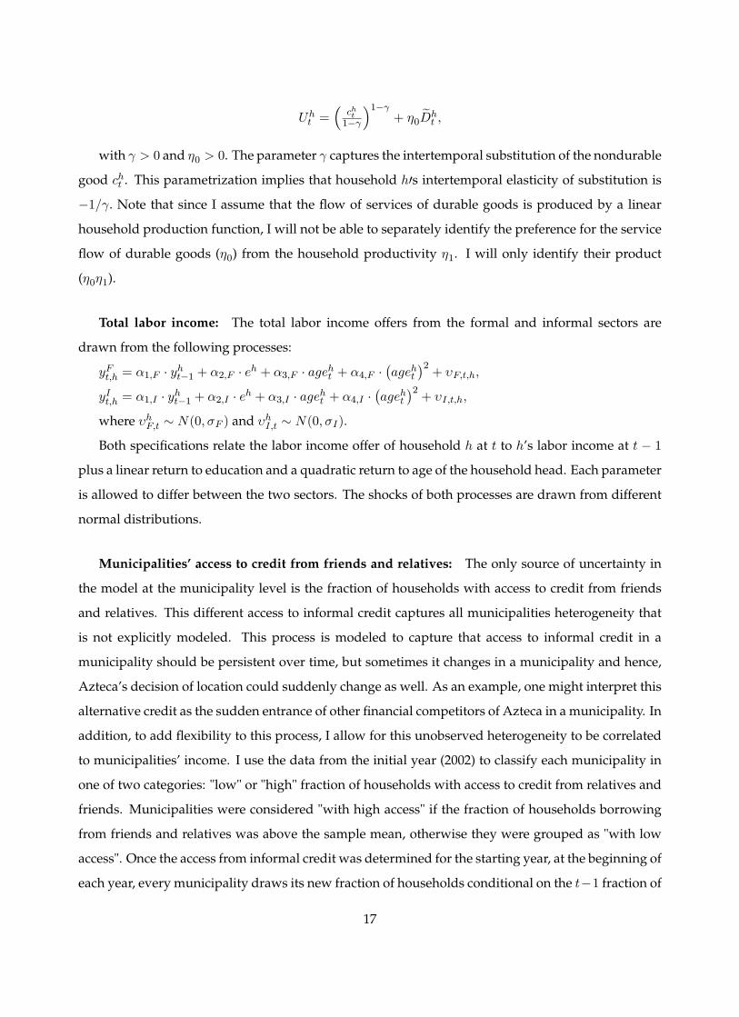
Uht =�cht1�

�1� + �0 eDht ;

with > 0 and �0 > 0. The parameter captures the intertemporal substitution of the nondurable

good cht . This parametrization implies that household h0s intertemporal elasticity of substitution is

�1= . Note that since I assume that the flow of services of durable goods is produced by a linear

household production function, I will not be able to separately identify the preference for the service

flow of durable goods (�0) from the household productivity �1. I will only identify their product

(�0�1).

Total labor income: The total labor income offers from the formal and informal sectors are

drawn from the following processes:

yFt;h = �1;F � yht�1 + �2;F � eh + �3;F � ageht + �4;F ��ageht

�2+ �F;t;h;

yIt;h = �1;I � yht�1 + �2;I � eh + �3;I � ageht + �4;I ��ageht

�2+ �I;t;h;

where �hF;t � N(0; �F ) and �hI;t � N(0; �I):

Both specifications relate the labor income offer of household h at t to h’s labor income at t � 1

plus a linear return to education and a quadratic return to age of the household head. Each parameter

is allowed to differ between the two sectors. The shocks of both processes are drawn from different

normal distributions.

Municipalities’ access to credit from friends and relatives: The only source of uncertainty in

the model at the municipality level is the fraction of households with access to credit from friends

and relatives. This different access to informal credit captures all municipalities heterogeneity that

is not explicitly modeled. This process is modeled to capture that access to informal credit in a

municipality should be persistent over time, but sometimes it changes in a municipality and hence,

Azteca’s decision of location could suddenly change as well. As an example, one might interpret this

alternative credit as the sudden entrance of other financial competitors of Azteca in a municipality. In

addition, to add flexibility to this process, I allow for this unobserved heterogeneity to be correlated

to municipalities’ income. I use the data from the initial year (2002) to classify each municipality in

one of two categories: "low" or "high" fraction of households with access to credit from relatives and

friends. Municipalities were considered "with high access" if the fraction of households borrowing

from friends and relatives was above the sample mean, otherwise they were grouped as "with low

access". Once the access from informal credit was determined for the starting year, at the beginning of

each year, every municipality draws its new fraction of households conditional on the t�1 fraction of

17

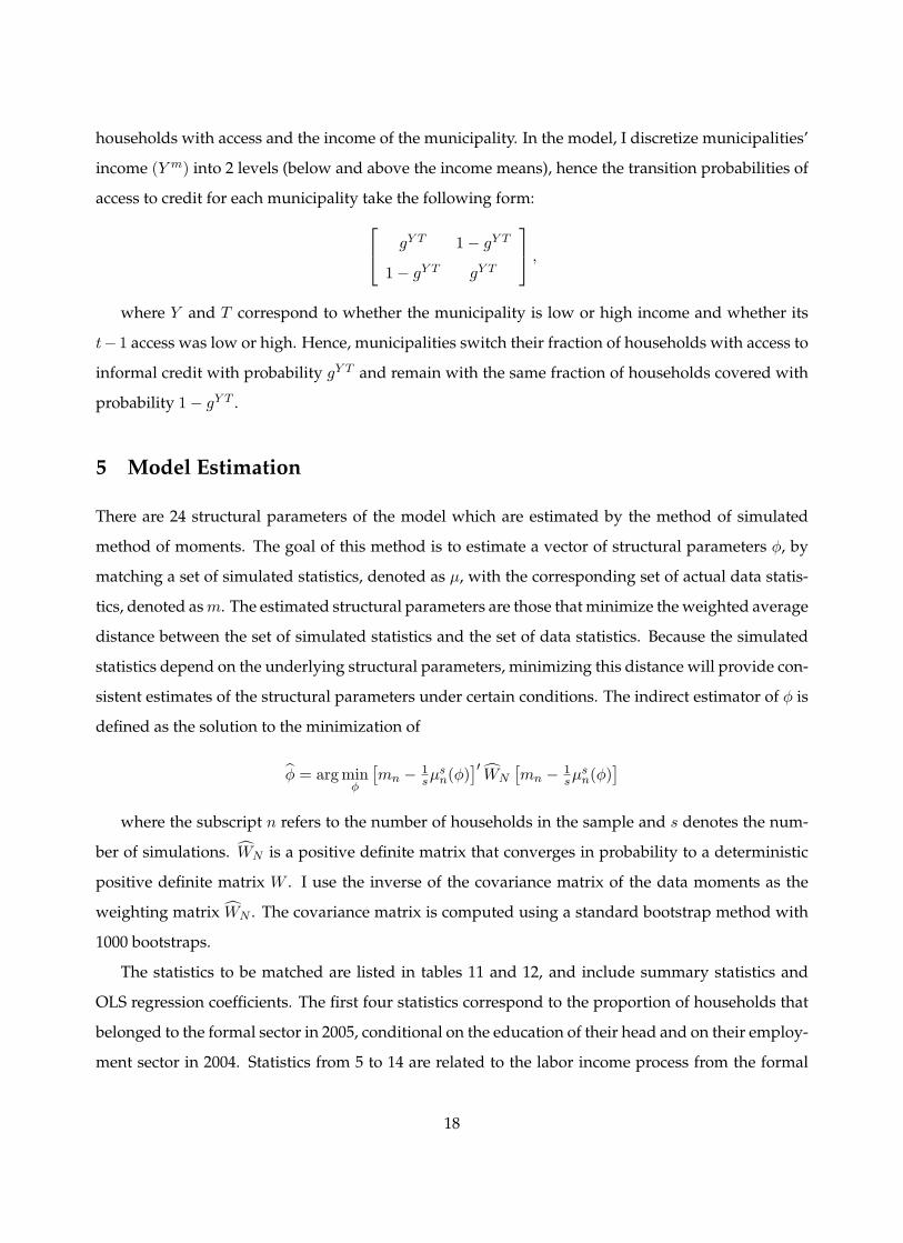
households with access and the income of the municipality. In the model, I discretize municipalities’

income (Y m) into 2 levels (below and above the income means), hence the transition probabilities of

access to credit for each municipality take the following form:24 gY T 1� gY T

1� gY T gY T

35 ;where Y and T correspond to whether the municipality is low or high income and whether its

t� 1 access was low or high. Hence, municipalities switch their fraction of households with access to

informal credit with probability gY T and remain with the same fraction of households covered with

probability 1� gY T .

5 Model Estimation

There are 24 structural parameters of the model which are estimated by the method of simulated

method of moments. The goal of this method is to estimate a vector of structural parameters �, by

matching a set of simulated statistics, denoted as �, with the corresponding set of actual data statis-

tics, denoted asm. The estimated structural parameters are those that minimize the weighted average

distance between the set of simulated statistics and the set of data statistics. Because the simulated

statistics depend on the underlying structural parameters, minimizing this distance will provide con-

sistent estimates of the structural parameters under certain conditions. The indirect estimator of � is

defined as the solution to the minimization of

b� = argmin�

�mn � 1

s�sn(�)

�0cWN

�mn � 1

s�sn(�)

�where the subscript n refers to the number of households in the sample and s denotes the num-

ber of simulations. cWN is a positive definite matrix that converges in probability to a deterministic

positive definite matrix W . I use the inverse of the covariance matrix of the data moments as the

weighting matrix cWN . The covariance matrix is computed using a standard bootstrap method with

1000 bootstraps.

The statistics to be matched are listed in tables 11 and 12, and include summary statistics and

OLS regression coefficients. The first four statistics correspond to the proportion of households that

belonged to the formal sector in 2005, conditional on the education of their head and on their employ-

ment sector in 2004. Statistics from 5 to 14 are related to the labor income process from the formal

18

and informal sectors4. Statistic 5 captures the persistence of labor income in the formal sector, by

regressing the 2005 labor income of formal households on their 2004 labor income. The next moment

captures the returns to education on the formal labor income by computing the mean difference be-

tween labor income of low and high educated households that belonged to the formal sector by 2005.

Moments 8 and 9 describe the income returns to age in the formal sector, by comparing the 2005 labor

income of households older and younger than 35 and households older and younger than 505, condi-

tional on being employed in the formal sector. Moment 10 captures the variance of the income shocks

received by formal households in 2005. These shocks are the residuals from the OLS regression of

formal labor income in 2005 on 2004 labor income, education, age and age squared for households

observed in the formal sector at 2005. The same statistics are used to capture the income process of

the informal sector (moments 10 to 14).

The next four moments relate to households’ consumption behavior. These moments correspond

to the 5th percentile of the distribution of households’ percapita expenditure in 2005; the proportion

of households that owned radio, TV sets, VCRs or computers in 2005; the 2005 ratio of percapita

expenditure to total income across households; and the log of the ratio of percapita expenditure in

2005 to the 2002 percapita expenditure across households. Moment 19 corresponds to the proportion

of municipalities that had an Azteca branch in 2005. The next two moments refer to informal credit

access. To compute them, I first obtained the 2005 average fraction of households with loans from

friends and relatives across municipalities. Moment 20 corresponds to the municipalities that were

below this average. It captures the mean proportion of households that got informal loans in these

municipalities. Moment 21 refers to the same statistic but using the sample of municipalities who

were above the average fraction of households with credit from friends or relatives. The last four

moments capture the persistence of credit from friends and relatives over time. I computed the

average fraction of households across municipalities that got credit from friends and relatives in

2002 and 2005, respectively. I then classified municipalities into two groups: municipalities below

the average fraction in 2002 and municipalities above. Moment 22 is the proportion of households

that in 2005 obtained an informal loan conditional on low-income municipalities that were below the

2002 mean of credit from friends and relatives. Moment 23 is the proportion of households that in

2005 obtained an informal loan conditional on low-income municipalities that were above the 2002

mean of credit from friends and relatives. Moment 24 is the proportion of households that in 2005

4The households’ data (MxFLS) includes retrospective information for the years 2004 and 2001 regarding labor deci-sions, which is used to compute these moments.

5In the model, the age of the household corresponds to the age of its head.

19

obtained an informal loan conditional on high-income municipalities that were below the 2002 mean

of credit from friends and relatives. Moment 25 is the proportion of households that in 2005 obtained

an informal loan conditional on high-income municipalities that were above the 2002 mean of credit

from friends and relatives.

6 Estimation results and model fit

The estimation of the model requires some choices regarding the size of the state space. I discretize

households’ savings and labor income, the value of the durable goods, the household head’s years of

schooling, the fraction of households covered by friends and relatives, and the income of the munic-

ipalities, which are the continuous state variables of the model. The grids were selected so that they

reflect the distributions of these variables in the data. The grid of savings consists of 10 points, the first

one equals the 5th percentile of the empirical savings distribution and the consecutive points refer to

the 15th, 25th,..., 85th and 95th percentiles. I tested the robustness of the simulations using fewer grid

points and I found that it is important to include at least 10 points. The value of the durable goods

was discretized to 4 point grids. The first point corresponds to a value of $0 and the last 3 points

reflect the empirical distribution of durable goods value: these points correspond to the 30th, 60th

and 90th percentiles of the data distribution. Household heads’ years of schooling were discretized

into two grid points: the first point corresponds to all household heads with less than 9 years of

schooling and the second point includes all households in which the head had 9 or more years of

education. At the aggregate level, municipalities were classified by their fraction of households with

access to credit from friends and relatives into two categories: below and above the mean fraction

of households who borrowed from friends and relatives. Municipalities were also classified in two

groups according to their percapita income, using the median income as the cut-off. Households’

labor income was also discretized using a 3-point grid, whose points correspond to the mean values

between the 1st and the 33th percentiles, the 33th and 66th percentiles and above the 66th percentile

of the distribution of total labor income. Finally, I approximate the discrete distributions of formal

and informal labor income shocks following Kennan (2006). I specify a continuous distribution for

each sector shock, and given the parameters of this distribution, I specify a discrete approximation to

them. I allow for 3 support points for these discrete approximations.

20

6.1 Estimation results

Table 13 presents the estimated parameters and their asymptotic standard errors. I compute the

asymptotic standard errors following Berndt, Hall, and Hall (1974) and Nash (1990).

Probability parameters of receiving a formal offer: fht j eh; F ht�1Since the probability that a household receives a formal-sector job offer depends on whether the

household belonged to the formal sector in the last period and on the education of the household

head, eh, the model estimates four different probabilities. According to the estimation results, the

probability of receiving an offer from the formal sector increases substantially if households were

formal in the previous period. For low and high educated households, the estimated probabilities are

0.627 and 0.793, respectively. Households employed in the informal sector have a lower probability

of receiving a formal job offer in the next period. These probabilities are 0.059 for low educated

households and 0.126 for high educated ones.

Parameters for formal labor income process: �1;F , �2;F , �3;F , �4;F , �F

The labor income process is allowed to depend linearly on previous labor income and education,

and concavely on age. The estimated persistence for the formal income is 0.5312, which means that

each period, households income consists of 53% of their lagged labor income. The returns to educa-

tion in the formal sector are estimated to 1.26. This coefficient implies that in the formal sector, income

of high-educated households is 45.5% higher than low educated households. Regarding returns to

age, the estimated coefficients are 0.04 and -0.0003. These parameters indicate that the age at which

a household employed in the formal sector receives its highest income is 66 years. The estimated

standard deviation of the income shocks from the formal sector is 2.305.

Parameters for informal labor income process: �1;I , �2;I , �3;I , �4;I , �I .

According to the estimated model, the persistence of lagged labor income on current income in

the informal sector is 0.48, lower than in the formal sector. The returns to education (0.7) imply that

relative to households with low education, the income of high-educated households in the informal

sector is 58% higher. The estimated coefficients on age are 0.02 and -0.00018, respectively. Compared

to the formal sector, the peak income age is reached earlier in the informal sector, when households

are 56 years old. The standard deviation of the informal income shocks is 2.52, slightly higher than

the variance from the formal sector.

Parameters for access to informal credit (credit from friends and relatives): Rmt

In the model, access to credit from friends and relatives varies among municipalities. For com-

21

putational reasons, municipalities are allowed to have two different types of access: low and high.

The estimated parameter for low access to informal credit is 0.05, which implies that in municipali-

ties with low access, only 5% of households can borrow from friends or relatives if they need to. In

municipalities with high coverage, each period 32.1% of households have a friend or relative from

which they can borrow.

Parameters for the transition of fraction of households with access to credit from friends and

relatives: gY T

The parameters ruling the transition over time of informal loans are as follows. Low-income mu-

nicipalities who had low access to informal credit in the previous period, stay with low access to

informal credit with probability 0.98, and experience high access with probability 0.02. If low-income

municipalities previously had high access to informal credit, they stay with high access with prob-

ability 0.502. For high-income municipalities, the transition probabilities are the following. Those

municipalities who had low access to informal credit in the previous period, stay with low access

with probability 0.927. Municipalities that experienced high access to credit in the past, would re-

main with high access at t with probability 0.934.

Households’ preferences parameters: , �0�1.

The estimated intertemporal substitution of nondurable goods, , is 3.1, which is within the range

of what other papers have found. The estimated joint product of �0�1 is 2.1 but given the parame-

trization, I am not able to identify separately the preference for the service flow of durable goods (�0)

from the household productivity �1.

Banco Azteca’s cost of operation: �.

The parameter for the Azteca’s cost of operation is estimated to 295. This parameter implies that

Azteca must pay each year $29; 500 USD to operate each branch.

Consumption floor.

This parameter determines the minimum consumption that a household receives. Its estimated

value is 0.4, which corresponds to a daily percapita consumption of $0:83USD.

Exogenous parameters. I now discuss the parameters that are not estimated inside the model.

Information about interest rates and collateral requirements is considered exogenous in the model.

Their values were obtained from CONDUSEF, Azteca’s Financial Reports and the households’ data.

According to this information, the average APRs of pawnshops, Banco Azteca, traditional banks and

friends or relatives over the years examined (2002 to 2005) were 220%, 130%, 40% and 0% respec-

tively. Regarding collateral, 90% of the households in the dataset that obtained credit from friends

22

and relatives reported they were not required to own any collateral, therefore in the model, the col-

lateral that friends and relatives require is set to zero. According to reports from PROFECO, the

average collateral required by a pawn shop in Mexico is six times the value of the loan. According to

CONDUSEF and Banco Azteca’s reports, both Banco Azteca and traditional banks require a collateral

equivalent to the value of the loan. The maximum loan that households can borrow from friends and

relatives is also determined outside the model. Its value is $2; 000USD, and was obtained from the

95th percentile of the distribution of loans from friends and relatives from the households data. The

depreciation of the durable goods, �, was fixed to 0.10. The relative price of the durable goods with

respect to the consumption goods, p, was obtained from the Consumer Price Index in 2002, and was

set to $10. The discount factor, �, was fixed to 0.99.

6.2 Model Fit

I now discuss the fit for the selected statistics in the estimation. In general, the estimated model

matches closely the simulated statistics to the real ones. Table 14 presents the moments for the share of

households employed in the formal sector in 2005, conditional on their education level and previous

sector employment. The likelihood of being employed in the formal sector is strongly correlated

with having participated in the formal sector in the previous period, for both low and high educated

households. But also, regardless of whether households were formal or not in the previous period,

education increases the probability of being formal. The simulated moments replicate these data

patterns closely. In general, the model fits well the labor income process of households employed

in the formal and informal sectors, as tables ?? and ?? show. The next table (table ??) presents other

households’ statistics. The simulated statistics for the 5th percentile of the distribution of households’

percapita consumption, the fraction of households who own durable goods and the consumption

moments are close to the data moments. The fit for the last statistics is listed in table 15. The model

slightly overpredicts the fraction of municipalities with an Azteca branch in 2005 (0.529 vs 0.51). The

simulated moments governing the behavior of credit from friends and relatives across municipalities

accurately fit the data patterns, and the persistence of the transitions of informal credit over time are

also replicated by the simulated statistics.

I now examine the performance of the model in predicting the type of municipalities where the

bank locates. Table 16 compares the characteristics of municipalities with Azteca between the simula-

tions and the real data. Information in the first column refers only to municipalities in which Azteca

operated from 2002 to 2005. The second column contains statistics only for municipalities where

23

Azteca located in 2002 but exited before 2005. The third column presents information of municipal-

ities where Azteca entered after 2002 but that by 2005 had an Azteca branch. The fourth column

contains information from municipalities where Azteca opened after 2002 and exited before 2005.

Finally, the fifth column presents statistics for municipalities that never had an Azteca branch. The

table summarizes the following variables at the municipality level: percentiles from the population

size and percapita income distributions, a dummy indicator that equals 1 if the municipality has a

branch of other bank institution and the total number of municipalities that fall into each category.

The first panel of the table reports information from the real data and the second panel reports on

the simulated data. We see from the number of municipalities that the model underpredicts munic-

ipalities where Azteca operated all periods (63 vs 48) and where Azteca never entered (67 vs 53);

and overpredicts the number of municipalities where Azteca entered from 2002 and exited before

2005 (2 vs 6), municipalities where Azteca entered after 2002 but stayed until at least 2005 (4 vs 24)

and municipalities where Azteca entered after 2002 and exited before 2005 (0 vs 5). However, the

overall pattern of bank branches, distribution of population size and percapita income are matched

substantially well.

7 Robustness of the model

To examine the performance of the model in reproducing the data patterns that were not used to

estimate the structural parameters, I examine if the model can reproduce the change experienced by

households from the informal sector in municipalities where Azteca located its branches. To do this, I

estimate difference-in-difference regressions in the real and simulated data in which the treated group

consists of informal households in municipalities with Azteca branches in 2005. Informal households

from all other municipalities are the control group. The regressions compare informal households’

outcomes of 2002 (before Azteca existed) with 2005 (once Azteca had operated for 3 years). The

outcomes examined refer to the probabilities that informal households obtained loans from banks

and from pawn shops, and the probability that these households saved.

Tables 17 to 19 present the results. The first column in the tables shows the real data difference-in-

difference specification. The second column presents the simulated difference-in-difference regres-

sion. The last column presents an alternative specification of the simulated difference-in-difference

regression. In the households data, the 1st percentile of bank and pawnshop loans is $30 USD and

$10 USD, respectively. Since in the model saving is a continuous variable, in this specification I con-

24

strain the simulated variables using these cutoffs. Hence, I consider that households borrowed from

banks/ pawnshops if they borrowed at least $30 USD/ $10 USD.

Table 17 presents the comparison of the difference-in-difference outcomes on the probability that

a household obtained a loan from banks. The coefficient of interest is the interaction of the variables

azteca (a dummy that equals one if the municipality had an Azteca over the period and zero other-

wise) and year (an indicator variable that equals one if the year is 2005 and 0 if the year is 2002), this

coefficient is denoted as azteca*year. According to the data patterns, informal households were more

likely to obtain bank loans once Azteca entered into their municipalities. This probability increased

in 0.0109, which implies an increase of more than 100% from their 2002 mean. The model is able to

reproduce this pattern, but it overestimates the size of the coefficient of interest. Once savings and

loans are constrained by the cutoffs from the real data, the simulated DID coefficient decreases to

0.0155, which is closer to the data coefficient.

Table 18 shows the probability that informal households obtained loans from pawnshops. Ac-

cording to the real data, relative to informal households from municipalities where Azteca did not

open during all periods, this probability declined in 0.011 points for informal households in munici-

palities with Azteca branches, which corresponds to a reduction of 50% in the mean pawnshop credit

usage of informal households by 2002. The model is able to reproduce this pattern, but underesti-

mates the magnitude of the coefficient (0.0038 which corresponds to a decline of 36%).

Table 19 shows the probability that informal households save. In the real data, this probability

is -0.031, which implies that the proportion of informal households who saved declined once Azteca

located its branches in their municipalities, relative to informal households from other municipalities.

Simulations of the model capture that the probability of saving declined in municipalities where

Azteca entered. Although the magnitude of the simulated DID is larger (0.12 vs 0.03), compared to

the 2002 mean, the percentage change in municipalities with Azteca is similar in the model to that in

the data (14% vs 11%).

8 Quantification of the Impact of Banco Azteca

8.1 Estimating the Impact of Banco Azteca on households’ outcomes

The estimated model suggests that the presence of Azteca alters households’ decisions regarding

credit, savings and durable goods acquisition, and also enhances households’ consumption smooth-

ing. In this section I discuss which households concentrate these effects and quantify the size of these

25

changes. I quantify the effects of Banco Azteca only on households from municipalities where Azteca

decided to enter. To do this, I compare the model simulations with simulations in which Azteca never

operates branches.

Saving patterns Figure 1 describes the average savings of households at different income deciles

under two cases: with and without Azteca. According to this table, once Azteca’s credit is available

in municipalities, lower income households decide to save less. Moreover, figure 2 shows that the

fraction of households saving also declines with the presence of this bank. On average, the frac-

tion of households saving declined by 5:8%. Regarding credit choices, figures ?? and ?? present the

share of households obtaining loans from Banco Azteca and pawnshops across income deciles. From

these figures we first see that usage of Azteca and pawnshop loans is concentrated among lower in-

come households. Additionally, once Azteca’s branches are available in the municipality, the share

of households borrowing from pawn shops declined.

Consumption of Durable and Nondurable goods Figure 5 presents the average value of durable

goods across income deciles with and without Azteca’s presence. The value of durable goods owned

by low-income households is higher in simulations that allow for Azteca branches. Consumption of

nondurable goods, however, remains unchanged once Azteca operates its branches.

Consumption Smoothing I now discuss whether households are better able to smooth their

consumption from income fluctuations over time, when credit from Azteca is available in their mu-

nicipalities. To analyze consumption smoothing of households over time, I adapt the index proposed

in Mazzocco and Saini (2008). The consumption smoothing index is defined as follows:

I = V ar(yh)�V ar(ch)V ar(yh)

;

where V ar(yh) and V ar(ch) correspond to the labor income and consumption variances of house-

hold h over time. This index (I) takes values from 0 to 1. See for example the extreme case in which

households’ consumption equals their labor income each period. In this case the numerator would

equal zero, and hence, I = 0. If households smooth their consumption entirely, then each period

households would consume the same amount, V ar(ch) would equal zero and I = 1. Therefore, the

higher the index, the better able are households smoothing their consumption. Table 22 presents the

mean of this index for households with and without Banco Azteca. Households’ index is 0:168when

the model is simulated without Azteca in their municipalities. When I simulate the model allowing

26

for the presence of Azteca, households’ consumption smoothing index increases to 0:19, implying an

increase of the index of 12%:

8.2 Difference-in-difference estimates using control group vs simulated treatment group

with no Azteca intervention

Since the entrance of Banco Azteca did not occur randomly across municipalities, difference-in-

difference (DID) estimations that compare municipalities chosen by the bank with other municipali-

ties are likely to be biased if we fail to account for all the observable and unobservable characteristics

that made Azteca decide its location. One advantage of the model is that it can be used to measure

this bias. To do this, I use the simulated data to estimate DID regressions using as a control group:

households from municipalities that did not have an Azteca branch by 2005 and households from the

same municipalities where Azteca entered under the scenario that Azteca never entered. To measure

the size of the bias, I then compare the DID estimates. I now discuss the results.

Tables 20 and 21 compare the simulated DID regressions. In both regressions, the treated group

is the same: informal households from municipalities with Azteca branches in 2005. The control

groups are different. The first column shows the DID specifications using as control group informal

households from municipalities without Azteca in 2005. DID estimates using the second control

group are shown in column 2. This alternative control group consists of informal households from

municipalities chosen by Azteca under the scenario that Azteca never entered. The second control

group must be the adequate control, since it consists of the same households but without Azteca’s

presence. According to the model results, using the correct control group yields lower estimates on

the DID results than using households from other municipalities where Azteca never entered. These

results suggest that comparing households from municipalities with Azteca with households from

municipalities without the bank might overestimate the real impact of Banco Azteca, since in the

absence of this bank, households from the treated municipalities were less likely to use pawnshops

loans and keep savings than households from municipalities where Azteca chose never to open.

9 Policy Evaluation

I now discuss the policy experiment, which consists of capping the interest rate that Banco Azteca

charges and examine how Azteca’s location choices change. Capping the interest rates of formal

credit institutions has been suggested by several Mexican policy makers who are opposed to exces-

27

sive interest rates charged to households. This policy however, could have the unintended effect of

making Azteca re-locate its branches and exit from municipalities where it currently operates. As the

model includes Azteca’s location choices, it is well suited to analyze this issue.

I simulate the model at different APRs charged by Azteca to examine changes in household credit

requests, average loan size and Banco Azteca selection of municipalities. In the model, Azteca locates

in municipalities based on its expected profits, which depend on households’ demand for Azteca’s

loans. The number of households that obtain Azteca’s credit and the amount borrowed by these

households must react to different APRs. Therefore, driven by these responses, Azteca’s selection of

municipalities can change.

I now discuss how households’ demand for Azteca’s credit reacts as the APR declines. Figure

10 presents the average size of loans conditional on obtaining Azteca’s credit and the proportion of

households that use Azteca’s credit at different APRs. As the APR declines, the fraction of house-

holds requesting Azteca’s credit increases. At an APR of 130%, 5:7% of households obtain credit

from Azteca, while at an APR of 40%, this number increases to 10:1%. Using the midpoint elasticity

formula, the extensive price elasticity of demand for Azteca’s credit is �0:52. We can see from the

figure that the average size of loans for households that obtain credit from Azteca is also sensitive

to changes in the APR. The average loan of households borrowing from Azteca at an APR of 130%

is $76:2 USD. This average increases to $105:5 USD when the APR charged is 40%. These results

indicate that the elasticity of loan size with respect to price is �:304. These results are comparable to

Karlan and Zinman (2008) who under a completely different setting found from a randomized trial

in South Africa an extensive elasticity of demand for consumer credit of �0:28 and a price elasticity

of loan size demand of �0:11. Although the elasticities that I find are larger, they are consistent with

an inelastic response of households to changes in the price of credit.

At the current APR, Azteca locates in 0.51 of all municipalities. However, as the APR that Azteca

charges decreases, the number of municipalities with Azteca’s branches falls (Figure 11). At an APR

of 40%, which represents a plausible ceiling since it is closer to traditional banks’ rates, Azteca would

only open in 44% of the sampled municipalities. Figures 12 and 13 provide information regarding

the average population size and percapita income of municipalities where Azteca would locate at

different APRs. As seen in Figure 12, As Azteca’s APR decreases, the average population size of

municipalities with Banco Azteca increases. This implies that at lower APRs, Azteca would exit from

less populated municipalities and would locate in the more populated ones. The same pattern is

observed when examining the percapita income of municipalities with Azteca’s branches. At lower

28

APRs, Azteca’s branches would concentrate in wealthier municipalities. Altogether, these results

suggest that if Banco Azteca were forced to charge lower rates and no other adjustment is done,

households from poorer and smaller municipalities would lose their Azteca branches.

10 Conclusions

This paper examined the impact of expanding access to credit on the decisions and welfare of house-

holds. To do so, the paper focused on the opening of Banco Azteca, the first bank in Mexico that

targeted households whose members belong to the informal sector. A comparison of household out-

comes from municipalities where this bank opened with other municipalities suggests that house-

holds, especially those employed in the informal sector, experienced significant changes in their sav-

ing, credit and consumption patterns. In order to address the impact of Banco Azteca and the issue

of endogenous location of its branches, I developed a model of household choices in which the bank

endogenously selects municipalities for branch openings.

I used the model to quantify the impact of Banco Azteca. I find substantial effects on house-

hold saving and consumption decisions once access to credit is available. First, households increased

their bank credit usage and decreased loans from other more expensive suppliers, such as pawn

shops. Second, in municipalities with presence of Azteca branches, the fraction of households saving

declined. These effects were sharper for households at lower income deciles, and suggest that the

use of savings as a buffer on income fluctuations declined once formal credit was available. Simu-

lations of the model indicate that consumption smoothing improved once households had access to

credit from Azteca. Consistent with the targeted population of Banco Azteca, informal households

experienced most changes.

I then use the estimated model to evaluate the effect of capping the APR that Azteca currently

charges on household demand for credit and Azteca’s location choices. Several policy makers in

Mexico have suggested imposing a ceiling on the interest rates of formal credit institutions in order

to make loans more affordable to people. The model simulations indicate that if the APR that Azteca

charges were capped to 40%, both the fraction of households obtaining Azteca loans and the aver-

age loan size of those borrowing would increase. Nevertheless, this increase in demand would not

compensate for the reduction in APR, and 14% of municipalities that currently have branches of this

bank would lose them. The likelihood of losing a branch is higher for poorer and less populated

municipalities.

29

References

Banerjee, A., E. Duflo, R. Glennerster, and C. Kinnan (2009). The miracle of microfinance. Evidence

from a randomized evaluation.

Bruhn, M. and I. Love (2009). The economic impact of banking the unbanked: evidence from Mexico.

Policy Research Working Paper Series.

Burgess, R. and R. Pande (2005). Do rural banks matter? Evidence from the Indian social banking

experiment. American Economic Review 95(3), 780–795.

Gourieroux, C. and A. Monfort (1996). Simulation-based econometric methods. Oxford University Press,

USA.

Gourieroux, C., A. Monfort, and E. Renault (1993). Indirect inference. Journal of Applied Economet-

rics 8(S1), S85–S118.

Kaboski, J. and R. Townsend (2008). A Structural Evaluation of a Large% Scale Quasi% Experimental

Microfinance Initiative.

Karlan, D. and J. Zinman (2008). Credit elasticities in less-developed economies: Implications for

microfinance. The American Economic Review 98(3), 1040–1068.

Keane, M. and K. Wolpin (1994). The solution and estimation of discrete choice dynamic program-

ming models by simulation and interpolation: Monte Carlo evidence. The Review of Economics and

Statistics, 648–672.

Kennan, J. (2006). A note on discrete approximations of continuous distributions. University of Wis-

consin Madison.

Mazzocco, M. and S. Saini (2008). Testing Efficient Risk Sharing with Heterogeneous Risk Preferences.

Department of Economics, University of Wisconsin at Madison Working Paper.

30

Table 1: Characteristics of municipalities by presence of Banco Azteca

All muns with muns with muns with muns withoutVariable muns Azteca Azteca from Azteca after Azteca’s

from 02 to 05 02 before 05 02 until 05 branches

Population size

p10 9; 413 57; 375 62; 773 47; 106 4; 318p25 19; 475 78; 512 62; 773 50; 168 10; 644p50 59; 675 227; 026 63; 319 57; 602 19; 447p75 226; 642 516; 255 63; 864 366; 068 41; 402p90 609; 829 1; 110; 997 63; 864 670; 162 69; 381

Percapita Income

p10 18; 789 31; 642 48; 436 25; 375 15; 100p25 28; 687 38; 561 48; 436 26; 349 22; 908p50 37; 136 50; 912 48; 876 31; 308 30; 434p75 54; 551 66; 846 49; 317 57; 985 37; 044p90 71; 967 76; 379 49; 317 80; 676 50; 423

Other banks 0:71 0:98 1:00 1:00 0:43# muns 136 63 2 4 67

Table reports population size and percapita income percentiles (10th,25th,50th,75th,90th)of the 136 municipalities of the sample, and the fraction of municipalities with presence ofbranches from other banks. Data from Mexican Economic Census and CNBV.

31

Table 2: Households’ Descriptive Statistics

Azteca No Azteca

Number of households2002 3,483 2,1562005 3,470 2,146

Fraction of formal hhds2002 0.238 0.131

(0.426) (0.337)2005 0.229 0.125

(0.421) (0.331)

Fraction of hhds who experienced:Death of a family member2002 0.010 0.014

(0.098) (0.116)2005 0.013 0.024

(0.113) (0.154)

Serious illness of a family member2002 0.024 0.021

(0.154) (0.144)2005 0.028 0.022

(0.164) (0.148)

Unemployment or failure of family business2002 0.050 0.028

(0.218) (0.164)2005 0.044 0.036

(0.206) (0.187)Table reports means and standard deviations (in parenthesis) of households’characteristics from municipalities with and without an Azteca branch in 2005.

32

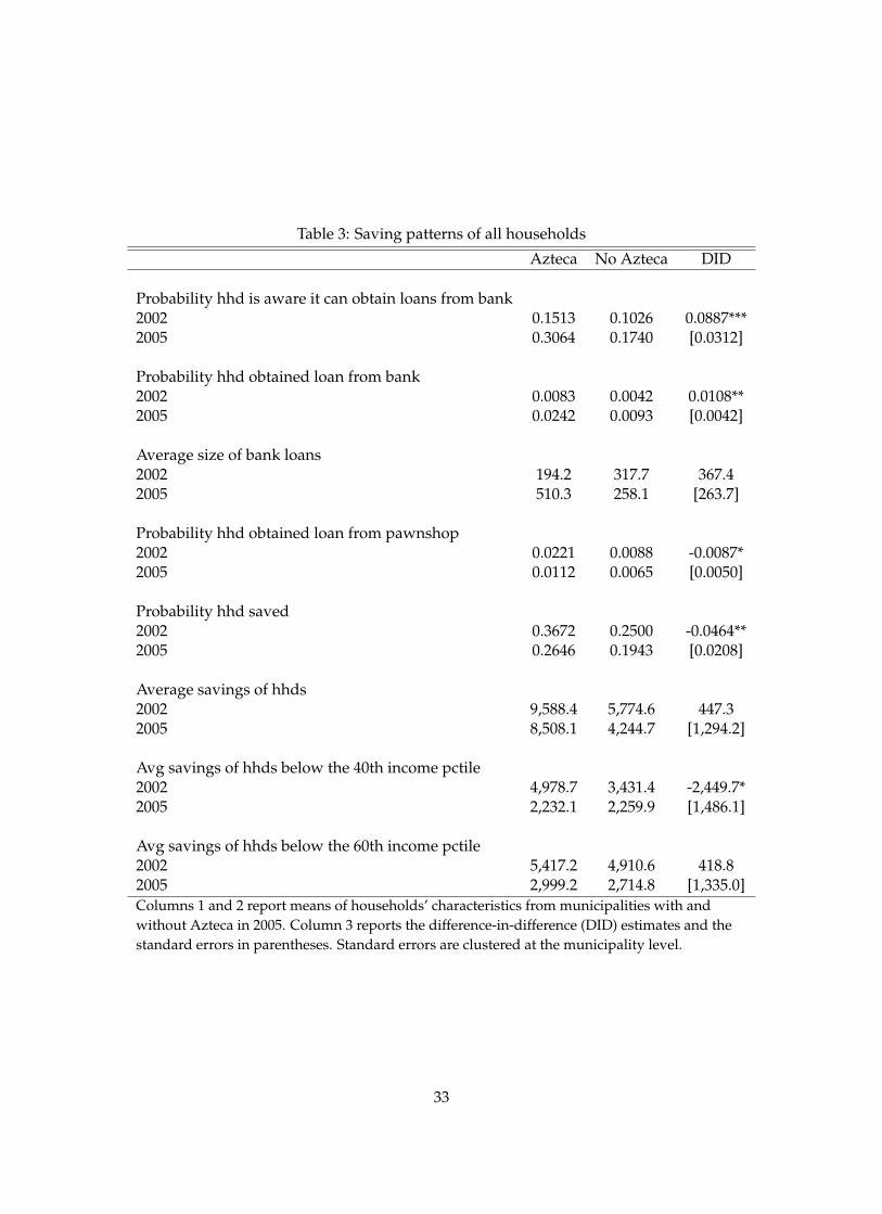
Table 3: Saving patterns of all households

Azteca No Azteca DID

Probability hhd is aware it can obtain loans from bank2002 0.1513 0.1026 0.0887***2005 0.3064 0.1740 [0.0312]

Probability hhd obtained loan from bank2002 0.0083 0.0042 0.0108**2005 0.0242 0.0093 [0.0042]

Average size of bank loans2002 194.2 317.7 367.42005 510.3 258.1 [263.7]

Probability hhd obtained loan from pawnshop2002 0.0221 0.0088 -0.0087*2005 0.0112 0.0065 [0.0050]

Probability hhd saved2002 0.3672 0.2500 -0.0464**2005 0.2646 0.1943 [0.0208]

Average savings of hhds2002 9,588.4 5,774.6 447.32005 8,508.1 4,244.7 [1,294.2]

Avg savings of hhds below the 40th income pctile2002 4,978.7 3,431.4 -2,449.7*2005 2,232.1 2,259.9 [1,486.1]

Avg savings of hhds below the 60th income pctile2002 5,417.2 4,910.6 418.82005 2,999.2 2,714.8 [1,335.0]Columns 1 and 2 report means of households’ characteristics from municipalities with andwithout Azteca in 2005. Column 3 reports the difference-in-difference (DID) estimates and thestandard errors in parentheses. Standard errors are clustered at the municipality level.

33

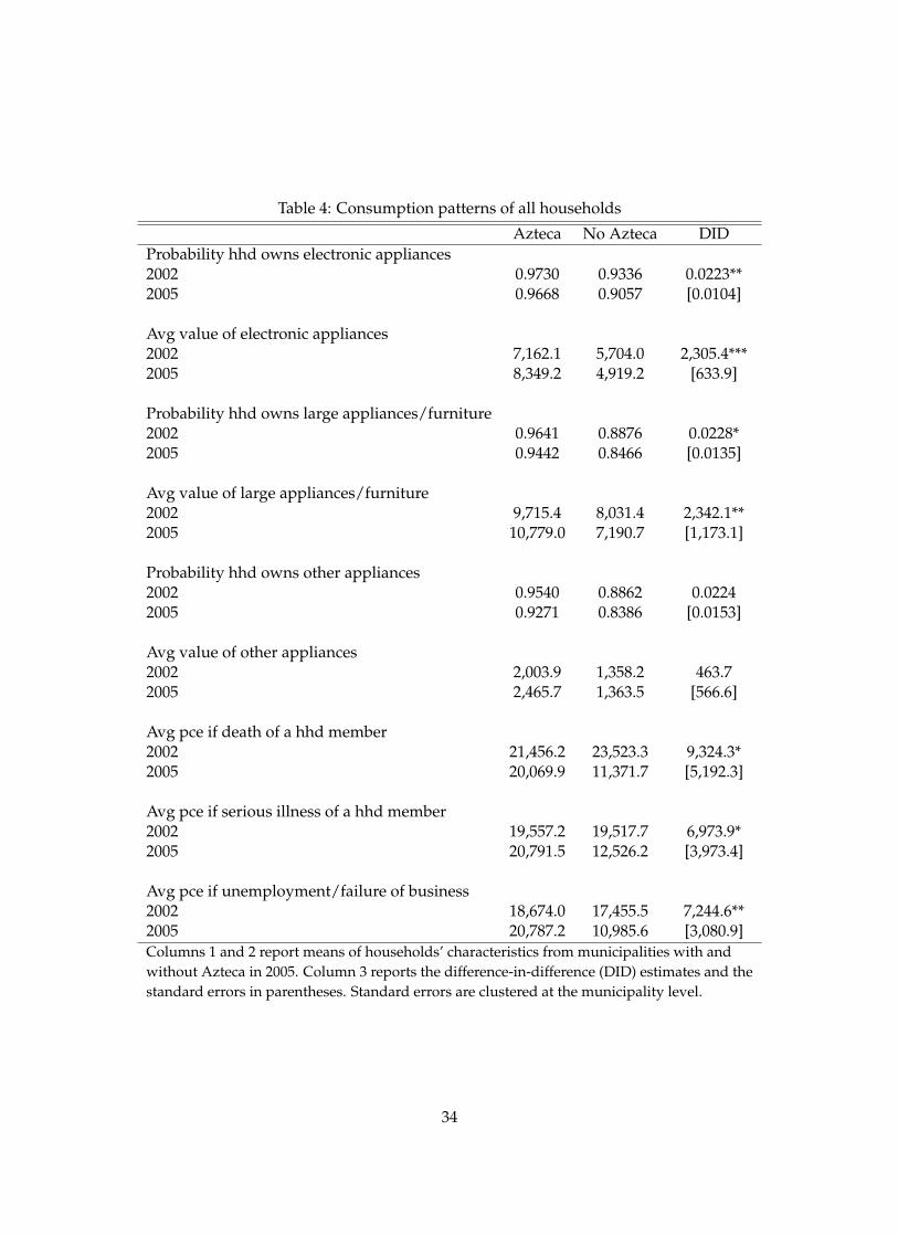
Table 4: Consumption patterns of all households

Azteca No Azteca DIDProbability hhd owns electronic appliances2002 0.9730 0.9336 0.0223**2005 0.9668 0.9057 [0.0104]

Avg value of electronic appliances2002 7,162.1 5,704.0 2,305.4***2005 8,349.2 4,919.2 [633.9]

Probability hhd owns large appliances/furniture2002 0.9641 0.8876 0.0228*2005 0.9442 0.8466 [0.0135]

Avg value of large appliances/furniture2002 9,715.4 8,031.4 2,342.1**2005 10,779.0 7,190.7 [1,173.1]

Probability hhd owns other appliances2002 0.9540 0.8862 0.02242005 0.9271 0.8386 [0.0153]

Avg value of other appliances2002 2,003.9 1,358.2 463.72005 2,465.7 1,363.5 [566.6]

Avg pce if death of a hhd member2002 21,456.2 23,523.3 9,324.3*2005 20,069.9 11,371.7 [5,192.3]

Avg pce if serious illness of a hhd member2002 19,557.2 19,517.7 6,973.9*2005 20,791.5 12,526.2 [3,973.4]

Avg pce if unemployment/failure of business2002 18,674.0 17,455.5 7,244.6**2005 20,787.2 10,985.6 [3,080.9]Columns 1 and 2 report means of households’ characteristics from municipalities with andwithout Azteca in 2005. Column 3 reports the difference-in-difference (DID) estimates and thestandard errors in parentheses. Standard errors are clustered at the municipality level.

34

Table 5: Saving patterns of informal households

Azteca No Azteca DID

Probability hhd is aware it can obtain loans from bank Azt No Azt DD2002 0.1322 0.0966 0.1009***2005 0.2761 0.1537 [0.0305]

Probability hhd obtained loan from bank2002 0.0064 0.0037 0.0139***2005 0.0232 0.0075 [0.0045]

Average size of bank loans2002 175.1 296.6 485.7*2005 519.0 209.9 [273.8]

Probability hhd obtained loan from pawnshop2002 0.0218 0.0069 -0.0105*2005 0.0105 0.0059 [0.0059]

Probability hhd saved2002 0.3337 0.2231 -0.0438*2005 0.2290 0.1677 [0.0230]

Average savings of hhds2002 9,000.3 4,969.2 -926.12005 6,396.4 2,975.4 [1,452.5]

Avg savings of hhds below the 40th income pctile2002 4,855.5 3,164.7 -2,264.7*2005 1,633.4 2,142.7 [1,239.7]

Avg savings of hhds below the 60th income pctile2002 5,142.7 4,173.7 257.32005 2,365.9 2,504.0 [1,526.7]Columns 1 and 2 report means of informal households’ characteristics from municipalities withand without Azteca in 2005. Column 3 reports the difference-in-difference (DID) estimates and thestandard errors in parentheses. Standard errors are clustered at the municipality level.

35

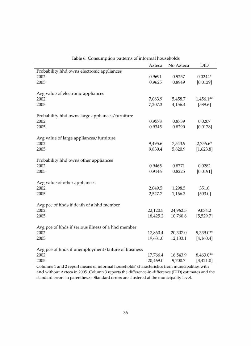
Table 6: Consumption patterns of informal households

Azteca No Azteca DIDProbability hhd owns electronic appliances2002 0.9691 0.9257 0.0244*2005 0.9625 0.8949 [0.0129]

Avg value of electronic appliances2002 7,083.9 5,458.7 1,456.1**2005 7,207.3 4,156.4 [589.6]

Probability hhd owns large appliances/furniture2002 0.9578 0.8739 0.02072005 0.9345 0.8290 [0.0178]

Avg value of large appliances/furniture2002 9,495.6 7,543.9 2,756.6*2005 9,830.4 5,820.9 [1,623.8]

Probability hhd owns other appliances2002 0.9465 0.8771 0.02822005 0.9146 0.8225 [0.0191]

Avg value of other appliances2002 2,049.5 1,298.5 351.02005 2,527.7 1,166.3 [503.0]

Avg pce of hhds if death of a hhd member2002 22,120.5 24,962.5 9,034.22005 18,425.2 10,760.8 [5,529.7]

Avg pce of hhds if serious illness of a hhd member2002 17,860.4 20,307.0 9,339.0**2005 19,631.0 12,133.1 [4,160.4]

Avg pce of hhds if unemployment/failure of business2002 17,766.4 16,543.9 8,463.0**2005 20,469.0 9,700.7 [3,421.0]Columns 1 and 2 report means of informal households’ characteristics from municipalities withand without Azteca in 2005. Column 3 reports the difference-in-difference (DID) estimates and thestandard errors in parentheses. Standard errors are clustered at the municipality level.

36

Table 7: Saving patterns of formal households

Azteca No Azteca DID

Probability hhd is aware it can obtain loans from bank2002 0.2121 0.1418 0.01472005 0.4056 0.3146 [0.0819]

Probability hhd obtained loan from bank2002 0.0145 0.0071 -0.01352005 0.0276 0.0224 [0.0203]

Average size of bank loans2002 262.2 468.6 -26.62005 479.5 622.1 [352.6]

Probability hhd obtained loan from pawnshop2002 0.0229 0.0213 0.01632005 0.0138 0.0112 [0.0213]

Probability hhd saved2002 0.4746 0.4291 -0.02142005 0.3844 0.3806 [0.0685]

Average savings of hhds2002 11,474.2 11,126.7 2,490.52005 15,575.6 13,120.7 [7,218.5]

Avg savings of hhds below the 40th income pctile2002 5,552.4 6,182.7 2,636.12005 5,718.0 3,681.2 [3,760.6]

Avg savings of hhds below the 60th income pctile2002 6,551.7 11,308.0 5,609.12005 5,993.5 4,959.5 [5,486.2]Columns 1 and 2 report means of formal households’ characteristics from municipalities withand without Azteca in 2005. Column 3 reports the difference-in-difference (DID) estimates and thestandard errors in parentheses. Standard errors are clustered at the municipality level.

37

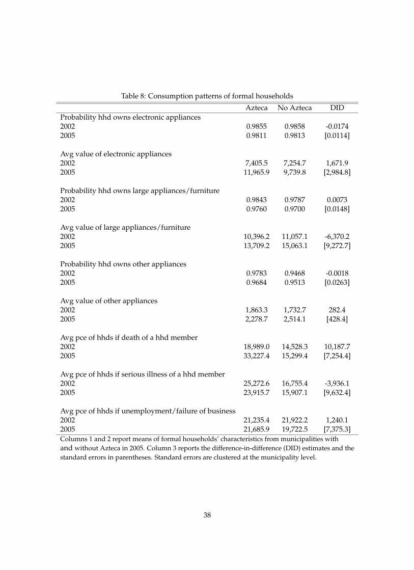
Table 8: Consumption patterns of formal households

Azteca No Azteca DIDProbability hhd owns electronic appliances2002 0.9855 0.9858 -0.01742005 0.9811 0.9813 [0.0114]

Avg value of electronic appliances2002 7,405.5 7,254.7 1,671.92005 11,965.9 9,739.8 [2,984.8]

Probability hhd owns large appliances/furniture2002 0.9843 0.9787 0.00732005 0.9760 0.9700 [0.0148]

Avg value of large appliances/furniture2002 10,396.2 11,057.1 -6,370.22005 13,709.2 15,063.1 [9,272.7]

Probability hhd owns other appliances2002 0.9783 0.9468 -0.00182005 0.9684 0.9513 [0.0263]

Avg value of other appliances2002 1,863.3 1,732.7 282.42005 2,278.7 2,514.1 [428.4]

Avg pce of hhds if death of a hhd member2002 18,989.0 14,528.3 10,187.72005 33,227.4 15,299.4 [7,254.4]

Avg pce of hhds if serious illness of a hhd member2002 25,272.6 16,755.4 -3,936.12005 23,915.7 15,907.1 [9,632.4]

Avg pce of hhds if unemployment/failure of business2002 21,235.4 21,922.2 1,240.12005 21,685.9 19,722.5 [7,375.3]Columns 1 and 2 report means of formal households’ characteristics from municipalities withand without Azteca in 2005. Column 3 reports the difference-in-difference (DID) estimates and thestandard errors in parentheses. Standard errors are clustered at the municipality level.

38

Table 9: DIDs of informal households using alternative treatment group

Azteca Azteca byin 05 06 or later

Probability hhd is aware it can obtain loans from bank2002 0.1009*** 0.0767*2005 [0.0305] [0.0420]

Probability hhd obtained loan from bank2002 0.0139*** 0.00962005 [0.0045] [0.0078]

Average size of bank loans2002 485.7* 283.62005 [273.8] [272.1]

Probability hhd obtained loan from pawnshop2002 -0.0105* -0.00182005 [0.0059] [0.0047]

Probability hhd saved2002 -0.0438* -0.01292005 [0.0230] [0.0487]

Average savings of hhds2002 -926.1 -3,051.52005 [1,452.5] [3,698.3]

Avg savings of hhds below the 40th income pctile2002 -2,264.7* -2,508.62005 [1,239.7] [2,232.8]

Avg savings of hhds below the 60th income pctile2002 257.3 -1879.92005 [1,526.7] [3,766.5]Table reports DID estimates and their standard errors in parentheses. Standarderrors are clustered at the municipality level.

39

Table 10: DIDs of informal households using alternative treatment group

Azteca Azteca byin 05 06 or later

Probability hhd owns electronic appliances2002 0.0244* 0.00172005 [0.0129] [0.0225]

Avg value of electronic appliances2002 1,456.1** -120.92005 [589.6] [920.4]

Probability hhd owns large appliances/furniture2002 0.0207 0.04592005 [0.0178] [0.0293]

Avg value of large appliances/furniture2002 2,756.6* 1,553.62005 [1,623.8] [2,000.8]

Probability hhd owns other appliances2002 0.0282 -0.03012005 [0.0191] [0.0326]

Avg value of other appliances2002 351.0 -902.402005 [503.0] [584.1]

Avg pce of hhds if death of a hhd member2002 9,034.2 -6,970.102005 [5,529.7] [12,020.3]

Avg pce of hhds if serious illness of a hhd member2002 9,339.0** -12,700.12005 [4,160.4] [7,801.8]

Avg pce of hhds if unemployment/failure of business2002 8,463.0** 5,707.12005 [3,421.0] [3,608.6]Table reports DID estimates and their standard errors in parentheses. Standarderrors are clustered at the municipality level.

40

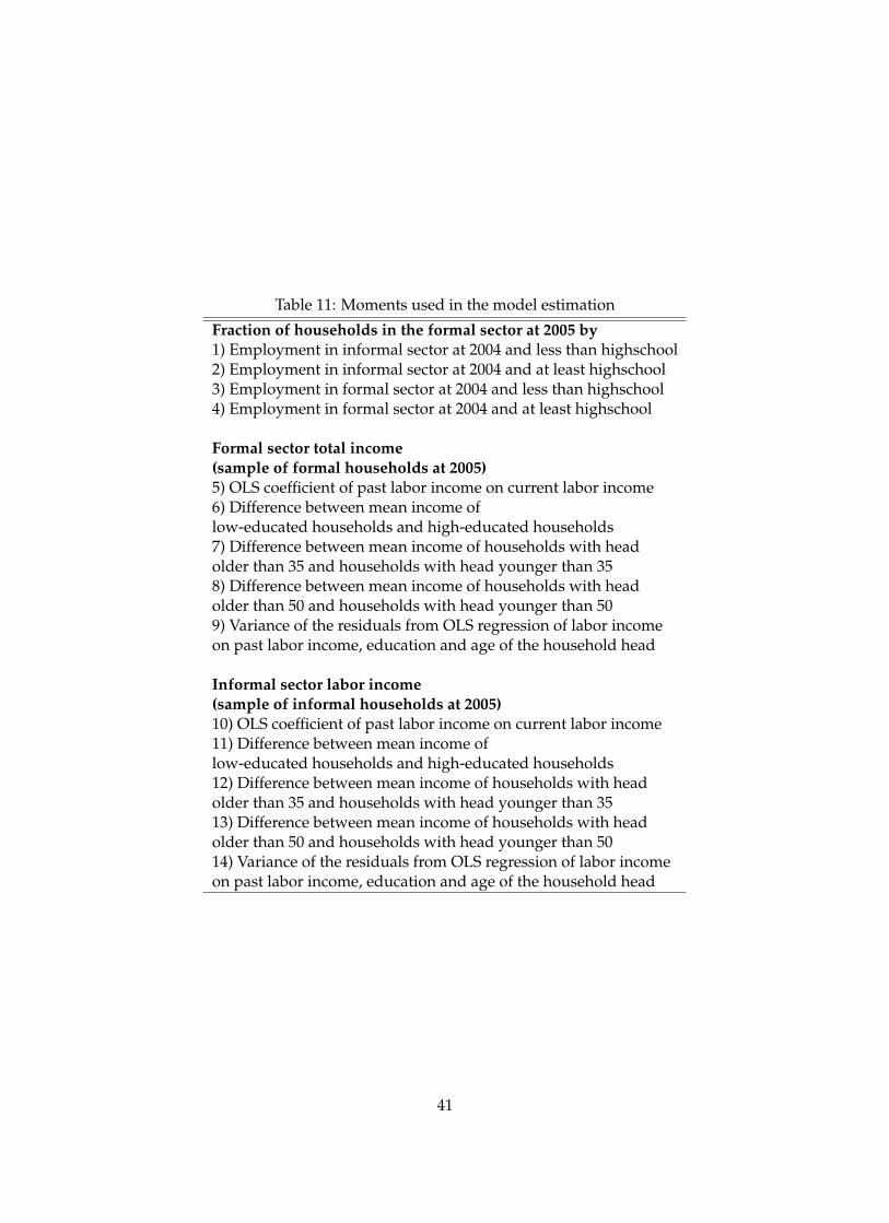
Table 11: Moments used in the model estimation

Fraction of households in the formal sector at 2005 by1) Employment in informal sector at 2004 and less than highschool2) Employment in informal sector at 2004 and at least highschool3) Employment in formal sector at 2004 and less than highschool4) Employment in formal sector at 2004 and at least highschool

Formal sector total income(sample of formal households at 2005)5) OLS coefficient of past labor income on current labor income6) Difference between mean income oflow-educated households and high-educated households7) Difference between mean income of households with headolder than 35 and households with head younger than 358) Difference between mean income of households with headolder than 50 and households with head younger than 509) Variance of the residuals from OLS regression of labor incomeon past labor income, education and age of the household head

Informal sector labor income(sample of informal households at 2005)10) OLS coefficient of past labor income on current labor income11) Difference between mean income oflow-educated households and high-educated households12) Difference between mean income of households with headolder than 35 and households with head younger than 3513) Difference between mean income of households with headolder than 50 and households with head younger than 5014) Variance of the residuals from OLS regression of labor incomeon past labor income, education and age of the household head

41

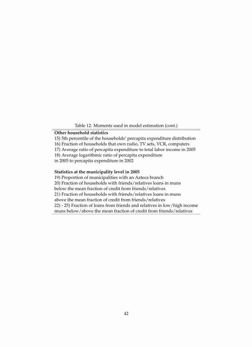
Table 12: Moments used in model estimation (cont.)

Other household statistics15) 5th percentile of the households’ percapita expenditure distribution16) Fraction of households that own radio, TV sets, VCR, computers17) Average ratio of percapita expenditure to total labor income in 200518) Average logarithmic ratio of percapita expenditurein 2005 to percapita expenditure in 2002

Statistics at the municipality level in 200519) Proportion of municipalities with an Azteca branch20) Fraction of households with friends/relatives loans in munsbelow the mean fraction of credit from friends/relatives21) Fraction of households with friends/relatives loans in munsabove the mean fraction of credit from friends/relatives22) - 25) Fraction of loans from friends and relatives in low/high incomemuns below/above the mean fraction of credit from friends/relatives

42

Table 13: Estimated parameters

param ASEProbability of job offer from the formal sectorLow educated households, informal sector at t-1 0:0589 0:00073Low educated households, formal sector at t-1 0:6269 0:01825High educated households, informal sector at t-1 0:1255 0:00053High educated households, formal sector at t-1 0:7927 0:00058

Labor income from the formal sectorPersistence of lagged labor income 0:5312 0:00189Returns to education 1:2698 0:00190Returns to age 0:0400 0:00041Returns to age squared �0:0003 0:00003St dev of residuals 2:3052 0:00304

Labor income from the informal sectorPersistence of lagged labor income 0:4800 0:00276Returns to education 0:7000 0:00401Returns to age 0:0200 0:00052Returns to age squared �0:0002 0:00004St dev of residuals 2:5200 0:00442

Credit from friends and relatives% households covered in muns with low access 0:0500 0:00025% households covered in muns with high access 0:3213 0:00070

Prob of high access to loans from friends/relativesIf low access at t-1 and low-income mun 0:0205 0:00002If high access at t-1 and low-income mun 0:5021 0:00329If low access at t-1 and high-income mun 0:0730 0:00010If high access at t-1 and high-income mun 0:9344 0:00207

Utility parametersIntertemporal substitution of the nondurable good 3:1000 0:00427Preference from durable goods service flow 2:1000 0:00235

Other parametersAzteca’s fixed cost 295 12:48consumption floor 0:4000 0:00384

Table reports the structural parameters (column 1) and their asymptotic standarderrors (column 2).

43

Table 14: Model Fit- Households’ moments in 2005

model dataFraction of hhds in the formal sectorconditional on:Informal at 2004 and low educated 0:043 0:046Informal at 2004 and high educated 0:459 0:515Formal at 2004 and low educated 0:108 0:109Formal at 2004 and high educated 0:731 0:714

labor income moments of formal households:OLS coefficient of yht on yht�1 0:488 0:432Returns on education 1:791 1:925Returns on age (if age � 35) 0:191 0:151Returns on age (if age � 50) �0:219 0:015Variance of OLS residuals of labor income regression 2:071 2:478

labor income moments of informal households:OLS coefficient of yht on yht�1 0:405 0:435Returns on education 1:035 0:876Returns on age (if age � 35) 0:132 0:027Returns on age (if age � 50) �0:170 �0:211Variance of OLS residuals of labor income regression 2:057 2:097

consumption moments of households:5th percentile of the hhds’ consumption 0:400 0:389Fraction of hhds that own durable goods 0:873 0:958Average ratio of ch2005 to yh2005 0:976 0:717Average log ratio of ch2005=y

h2005 �0:172 �0:130

44

Table 15: Model fit- Statistics at the municipality level in 2005

model data

fraction of municipalities with an Azteca branch in 2005 52:9% 51:0%

fraction of hhds with credit from friends:if mun’s fraction of loans from friends is below the mean 0:010 0:019if mun’s fraction of loans from friends is above the mean 0:092 0:104

fraction of friends loans at 2005 in low-income muns with:if mun’s fraction of loans from friends is below the mean 0:014 0:060if mun’s fraction of loans from friends is above the mean 0:034 0:086

fraction of friends loans at 2005 in high-income muns with:fraction below mean of informal credit in 2002 0:025 0:059fraction above mean of informal credit in 2002 0:059 0:061

45

Table 16: Municipalities characteristics by presence of Banco Azteca

Variable from 02 from 02 after 02 after 02 no Azteca’sto 05 before 05 until 05 before 05 branches

DATA

Population sizep10 57; 375 62; 773 47; 106 4; 318p25 78; 512 62; 773 50; 168 10; 644p50 227; 026 63; 319 57; 602 19; 447p75 516; 255 63; 864 366; 068 41; 402p90 1; 110; 997 63; 864 670; 162 69; 381

Percapita Incomep10 31; 642 48; 436 25; 375 15; 100p25 38; 561 48; 436 26; 349 22; 908p50 50; 912 48; 876 31; 308 30; 434p75 66; 846 49; 317 57; 985 37; 044p90 76; 379 49; 317 80; 676 50; 423

Other banks 0:98 1:00 1:00 0:43Number of muns 63 2 4 0 67

MODEL

Population sizep10 83; 537 2; 306 46; 053 34; 088 4; 318p25 137; 282 24; 447 55; 560 37; 418 9; 862p50 272; 307 50; 262 69; 449 43; 827 14; 952p75 549; 018 57; 375 208; 871 45; 272 23; 984p90 1; 001; 021 75; 059 1; 110; 997 47; 106 39; 308

Percapita Incomep10 30; 486 34; 981 27; 886 23; 987 13; 762p25 38; 695 38; 561 30; 556 25; 375 18; 789p50 54; 551 43; 355 36; 966 32; 488 29; 330p75 68; 009 49; 662 47; 912 33; 353 39; 024p90 80; 731 67; 674 70; 645 41; 873 51; 731

Other banks 1:00 0:83 0:96 0:80 0:32Number of muns 48 6 24 5 53

Panels compare the presence of Azteca branches between model simulations and realdata, by population size, percapita income of municipalities (10th,25th,50th,75th, 90thpercentiles) and presence of other bank branches.

46

Table 17: Probability informal households have a bank loan

data model 1 model 2

azteca �0:0108��� 0:0000 0:0000[0:0032] [0:0006] [0:0003]

year 0:0056� 0:0000 0:0000[0:0029] [0:0007] [0:0003]

azteca*year 0:0139��� 0:0716��� 0:0155���

[0:0045] [0:0009] [0:0004]

Constant �0:0086 �0:0000 �0:0000[0:0088] [0:0005] [0:0002]

Observations 8382 464290 464290R-squared 0:0078 0:0500 0:0106

Column 1 reports the DID regression of the real data.Columns 2 and 3 present the DIDs of the simulated datawithout and with bounds of the continuous variable.

Table 18: Probability informal households have a pawnshop loan

data model 1 model 2

azteca 0:0093��� �0:0005 �0:0003[0:0033] [0:0005] [0:0004]

year �0:0022 �0:0070��� �0:0035���[0:0028] [0:0005] [0:0004]

aztyear �0:0105� �0:0067��� �0:0038���[0:0059] [0:0007] [0:0006]

Constant 0:0334��� 0:0185��� 0:0117���

[0:0090] [0:0004] [0:0003]

Observations 8382 464290 464290R-squared 0:0052 0:0030 0:0012

Column 1 reports the DID regression of the real data.Columns 2 and 3 present the DIDs of the simulated datawithout and with bounds of the continuous variable.

47

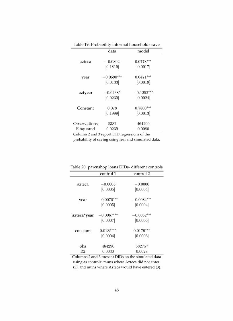
Table 19: Probability informal households save

data model

azteca �0:0892 0:0778���

[0:1819] [0:0017]

year �0:0590��� 0:0471���

[0:0133] [0:0019]

aztyear �0:0438� �0:1252���[0:0230] [0:0024]

Constant 0:078 0:7800���

[0:1999] [0:0013]

Observations 8382 464290R-squared 0:0239 0:0080

Column 2 and 3 report DID regressions of theprobability of saving using real and simulated data.

Table 20: pawnshop loans DIDs- different controls

control 1 control 2

azteca �0:0005 �0:0000[0:0005] [0:0004]

year �0:0070��� �0:0084���[0:0005] [0:0004]

azteca*year �0:0067��� �0:0052���[0:0007] [0:0006]

constant 0:0185��� 0:0179���

[0:0004] [0:0003]

obs 464290 582757R2 0:0030 0:0028

Columns 2 and 3 present DIDs on the simulated datausing as controls: muns where Azteca did not enter(2), and muns where Azteca would have entered (3).

48

Table 21: saving DIDs- different controls

control 1 control 2

azteca 0:0778��� 0:0000[0:0017] [0:0014]

year 0:0471��� �0:0096���[0:0019] [0:0014]

azteca*year �0:1252��� �0:0685���[0:0024] [0:0019]

constant 0:7800��� 0:8578���

[0:0013] [0:0010]

obs 464290 582757R2 0:0080 0:0078

Columns 2 and 3 present DIDs on the simulated datausing as controls: muns where Azteca did not enter(2), and muns where Azteca would have entered (3).

49

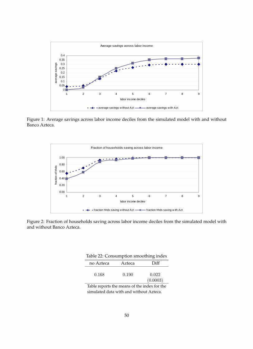
Average savings across labor income

00.050.1

0.150.2

0.250.3

0.350.4

1 2 3 4 5 6 7 8 9

labor income deciles

aver

age 

savi

ngs

average savings w ithout Azt average savings w ith Azt

Figure 1: Average savings across labor income deciles from the simulated model with and withoutBanco Azteca.

Fraction of households saving across labor income

0.00

0.20

0.40

0.60

0.80

1.00

1 2 3 4 5 6 7 8 9

labor income deciles

fract

ion 

of h

hds

f raction hhds saving w ithout Azt fraction hhds saving w ith Azt

Figure 2: Fraction of households saving across labor income deciles from the simulated model withand without Banco Azteca.

Table 22: Consumption smoothing index

no Azteca Azteca Diff

0:168 0:190 0:022(0:0003)

Table reports the means of the index for thesimulated data with and without Azteca.

50

Fraction of Azteca's loans across labor income

0.00

0.10

0.20

0.30

0.40

0.50

1 2 3 4 5 6 7 8 9

labor income deciles

fract

ion 

of h

hds

f raction of Azteca's loans

Figure 3: Fraction of households borrowing from Azteca across labor income deciles from the simu-lated model in municipalities where Banco Azteca located its branches.

Fraction of pawnshop loans across labor income

0.000

0.010

0.020

0.030

0.040

0.050

0.060

1 2 3 4 5 6 7 8 9

labor income deciles

aver

age 

savi

ngs

f raction paw nshop loans w ithout Azt fraction paw nshop loans w ith Azt

Figure 4: Fraction of households borrowing from pawnshops across labor income deciles from thesimulated model in municipalities where Banco Azteca located its branches.

51

Average value of durable goods across labor income

0.50.7

0.91.1

1.31.5

1.71.9

2.12.3

2.5

1 2 3 4 5 6 7 8 9

labor income decile

Ave

rage

 val

ue o

f dur

able

 goo

ds

without Azt  with Azt

Figure 5: Average value of durable goods across labor income deciles from the simulated model withand without Banco Azteca.

Average consumtion across labor income

0.5

1.5

2.5

3.5

4.5

5.5

6.5

7.5

8.5

1 2 3 4 5 6 7 8 9

labor income decile

Ave

rage

 con

sum

ptio

n

without Azt  with Azt

Figure 6: Average consumption of nondurable goods across labor income deciles from the simulatedmodel with and without Banco Azteca.

52

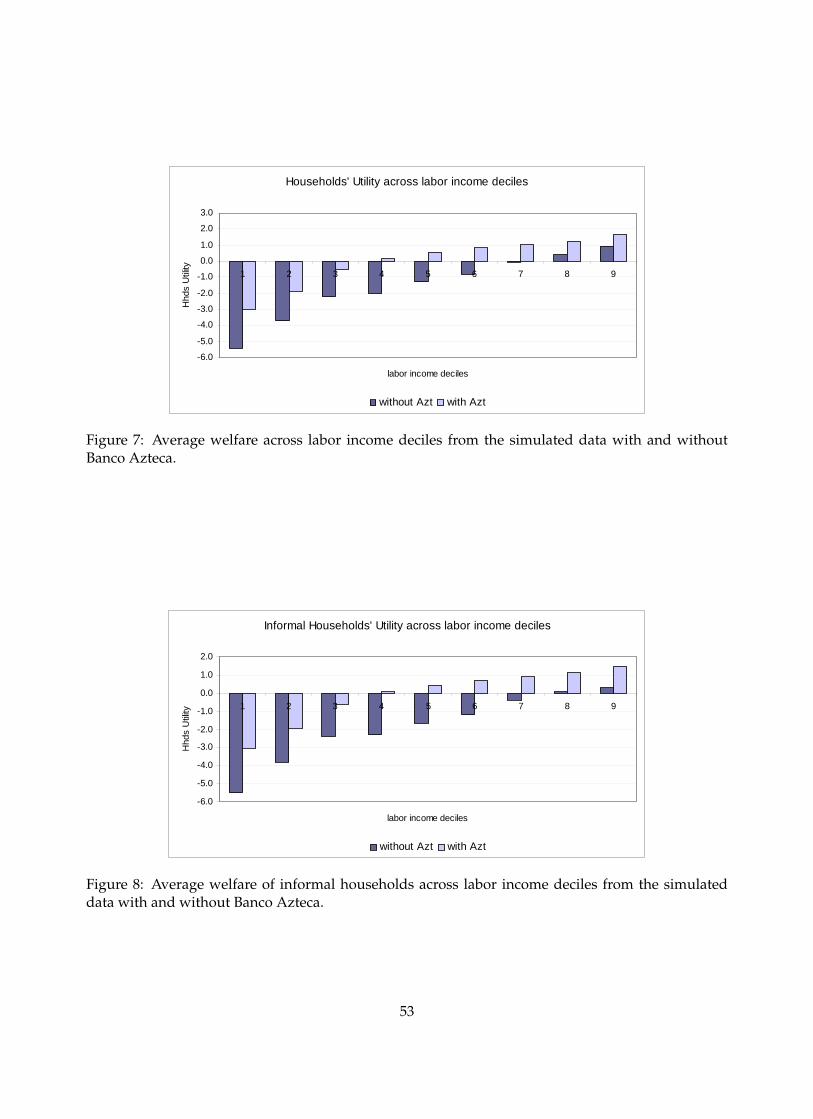
Households' Utility across labor income deciles

­6.0

­5.0

­4.0

­3.0

­2.0

­1.0

0.0

1.0

2.0

3.0

1 2 3 4 5 6 7 8 9

labor income deciles

Hhd

s U

tility

without Azt with Azt

Figure 7: Average welfare across labor income deciles from the simulated data with and withoutBanco Azteca.

Informal Households' Utility across labor income deciles

­6.0

­5.0

­4.0

­3.0

­2.0

­1.0

0.0

1.0

2.0

1 2 3 4 5 6 7 8 9

labor income deciles

Hhd

s U

tility

without Azt with Azt

Figure 8: Average welfare of informal households across labor income deciles from the simulateddata with and without Banco Azteca.

53

Formal Households' Utility across labor income deciles

­4.0

­3.0

­2.0

­1.0

0.0

1.0

2.0

3.0

1 2 3 4 5 6 7 8 9

labor income deciles

Hhd

s U

tility

without Azt with Azt

Figure 9: Average welfare of formal households across labor income deciles from the simulated datawith and without Banco Azteca.

0.000

20.000

40.000

60.000

80.000

100.000

120.000

40% 50% 60% 70% 80% 90% 100% 110% 120% 130%

Azteca's APR

Aver

age 

size

 of l

oans

0.000

0.020

0.040

0.060

0.080

0.100

0.120Pr

opor

tion 

of h

hds 

borr

owin

g

Average size of loans Proportion of hhds borrow ing

Figure 10: Left axis presents the average size of loans of households borrowing from Azteca at dif-ferent APRs. Right axis presents the proportion of households borrowing from Azteca at differentAPRs.

54

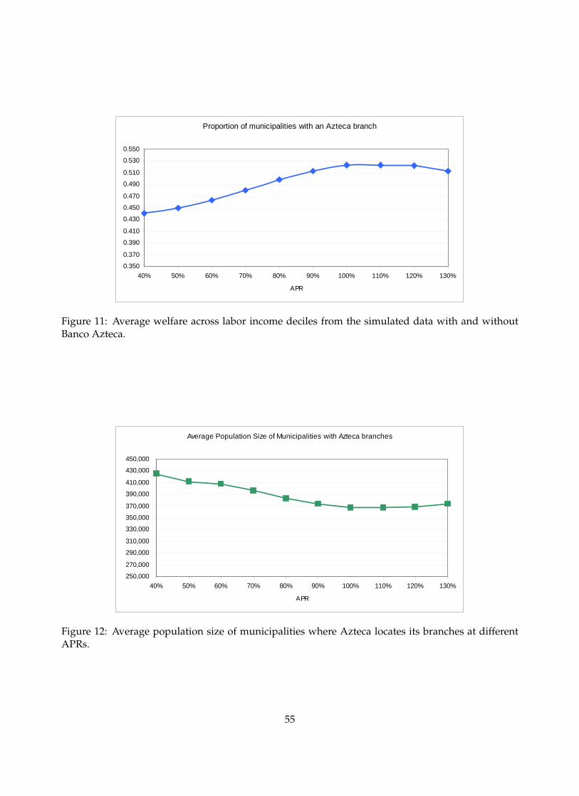
Proportion of municipalities with an Azteca branch

0.350

0.370

0.390

0.410

0.430

0.450

0.470

0.490

0.510

0.530

0.550

40% 50% 60% 70% 80% 90% 100% 110% 120% 130%

APR

Figure 11: Average welfare across labor income deciles from the simulated data with and withoutBanco Azteca.

Average Population Size of Municipalities with Azteca branches

250,000

270,000

290,000

310,000

330,000

350,000

370,000

390,000

410,000

430,000

450,000

40% 50% 60% 70% 80% 90% 100% 110% 120% 130%

APR

Figure 12: Average population size of municipalities where Azteca locates its branches at differentAPRs.

55

Average Percapita Income of Municipalities with Azteca branches

49,000

50,000

51,000

52,000

53,000

54,000

55,000

56,000

40% 50% 60% 70% 80% 90% 100% 110% 120% 130%

APR

Figure 13: Average percapita income of municipalities where Azteca locates its branches at differentAPRs.

56