From microscopic to macroscopic traffic patterns: different applications of the

variational theoryLudovic Leclercq

Université de Lyon, IFSTTAR / ENTPE, COSYS, LICIT

15

Traffic and Granular Flow’15

Outline

• Short historical review

– Micro to Macro for car-following models

– Recent results based on homogenisation technics

• The variational theory

• Applications to scaling-up problems

– Mean traffic states on urban corridors

– Capacity drops at merges

• Conclusion

2

SHORT HISTORICAL REVIEW

3

First micro to macro approaches (1)

• 1950-60: Herman, Gazis, Montroll, Chandler…

4

CHAPITRE 1. HOMOGENIZATION OF MICROSCOPIC TRAFFIC FLOW MODELS

where Q denotes the flow of vehicles. It is the simplest traffic flow model because it assumesthat the flow is always at a steady state of equilibrium. Many other macroscopic modelstried to improve this assumption of equilibrium by taking into account transitional trafficstates.

Microscopic to macroscopic approaches : One of the first micro-macro approachin traffic models was performed in the 1950’s and early 1960’s by researchers from theGeneral Motors Corporation, namely Robert Herman, Denos C. Gazis, Elliott W. Montrolland Robert E. Chandler among others. Indeed, they not only create car-following theory,they also make a link between such models and traffic flow ones. For instance, in [109],assuming that the leading vehicle in traffic stream has a constant speed u and integratingthe expression for the acceleration of (n + 1)st vehicle, it gives the expression for thevelocity of that vehicle, which in turn is intended to be the steady-state velocity of thetraffic stream. This velocity solves an appropriate equation mixing the flow and the density.

For example, consider the application of this procedure to the simplest linear car-following model

xn+1(t) = α [xn(t− T )− xn+1(t− T )]

giving the acceleration of (n + 1)st vehicle with respect to the relative speed modulo atime delay T > 0. By integration and up to a shift in time, we get the velocity

u := xn+1(t) = α[xn(t− T )− xn+1(t− T )! "# $

=:s=1ρ

] + C0.

The constant C0 can be computed thanks to the condition for null speed u = 0 obtainedat maximal density ρjam. Then from the definition of flow q = uρ, it proceeds that

q = α

%

1− ρ

ρjam

&

.

The constant α is given for the condition q(ρ = 0) = qm with qm = 0. It is noteworthy tounderline that this choice is not realistic for low densities or equivalently for high spacing,say that the car-following model is not consistent near to vacuum.

The same (formal) procedure could be used for other type of microscopic models. Forinstance, if doing so for the following model

xn+1(t + T ) = α0[xn(t)− xn+1(t)][xn(t)− xn+1(t)]l

[xn+1(t + T )]m

first proposed by Gazis, Herman and Rothery [109] and then examined by May and Keller[189], it follows the steady-state equations given in Table 1.1.

Macro-to-Micro approach is often based on a discretization of macroscopic modelsthanks to finite difference numerical schemes. The main one is Godunov scheme [117]which is equivalent in traffic to the Daganzo’s Cell Transmission model [76,77]. MoreoverGodunov numerical scheme has been translated into traffic through the notions of Supplyand Demand highlighted in [164].

In traffic literature, for micro-to-macro passage, the reader can refer to [10] which showsthat a particular time-discrete microscopic model converges to a second order macroscopicmodel, and to [157] where the macroscopic limit of a micro kinetic model is shown tobe equal to the Kruzhkov entropy solution of the LWR model. There is also the recentpaper [62]. The papers [208, 209] and [13] are more precisely dedicated to study stabilityproperties of microscopic models (and so their macroscopic behavior).

32 2. MICRO-TO-MACRO APPROACHES : A REVIEW

Car-following rule

=>

(+ steady state) =>

Not consistent for high spacings

s

v

s0

First micro to macro approaches (2)

CHAPITRE 1. HOMOGENIZATION OF MICROSCOPIC TRAFFIC FLOW MODELS

where Q denotes the flow of vehicles. It is the simplest traffic flow model because it assumesthat the flow is always at a steady state of equilibrium. Many other macroscopic modelstried to improve this assumption of equilibrium by taking into account transitional trafficstates.

Microscopic to macroscopic approaches : One of the first micro-macro approachin traffic models was performed in the 1950’s and early 1960’s by researchers from theGeneral Motors Corporation, namely Robert Herman, Denos C. Gazis, Elliott W. Montrolland Robert E. Chandler among others. Indeed, they not only create car-following theory,they also make a link between such models and traffic flow ones. For instance, in [109],assuming that the leading vehicle in traffic stream has a constant speed u and integratingthe expression for the acceleration of (n + 1)st vehicle, it gives the expression for thevelocity of that vehicle, which in turn is intended to be the steady-state velocity of thetraffic stream. This velocity solves an appropriate equation mixing the flow and the density.

For example, consider the application of this procedure to the simplest linear car-following model

xn+1(t) = α [xn(t− T )− xn+1(t− T )]

giving the acceleration of (n + 1)st vehicle with respect to the relative speed modulo atime delay T > 0. By integration and up to a shift in time, we get the velocity

u := xn+1(t) = α[xn(t− T )− xn+1(t− T )! "# $

=:s=1ρ

] + C0.

The constant C0 can be computed thanks to the condition for null speed u = 0 obtainedat maximal density ρjam. Then from the definition of flow q = uρ, it proceeds that

q = α

%

1− ρ

ρjam

&

.

The constant α is given for the condition q(ρ = 0) = qm with qm = 0. It is noteworthy tounderline that this choice is not realistic for low densities or equivalently for high spacing,say that the car-following model is not consistent near to vacuum.

The same (formal) procedure could be used for other type of microscopic models. Forinstance, if doing so for the following model

xn+1(t + T ) = α0[xn(t)− xn+1(t)][xn(t)− xn+1(t)]l

[xn+1(t + T )]m

first proposed by Gazis, Herman and Rothery [109] and then examined by May and Keller[189], it follows the steady-state equations given in Table 1.1.

Macro-to-Micro approach is often based on a discretization of macroscopic modelsthanks to finite difference numerical schemes. The main one is Godunov scheme [117]which is equivalent in traffic to the Daganzo’s Cell Transmission model [76,77]. MoreoverGodunov numerical scheme has been translated into traffic through the notions of Supplyand Demand highlighted in [164].

In traffic literature, for micro-to-macro passage, the reader can refer to [10] which showsthat a particular time-discrete microscopic model converges to a second order macroscopicmodel, and to [157] where the macroscopic limit of a micro kinetic model is shown tobe equal to the Kruzhkov entropy solution of the LWR model. There is also the recentpaper [62]. The papers [208, 209] and [13] are more precisely dedicated to study stabilityproperties of microscopic models (and so their macroscopic behavior).

32 2. MICRO-TO-MACRO APPROACHES : A REVIEW

Gazis, Herman and Rothery’s model:

@Gerlough and Huber,Traffic Flow Theory: a monograph, 1975

1967

Homogeneisation technics

A. Belkhabbaz et al. / Procedia Engineering 10 (2011) 1883–1888

A. Belkhabbaz et al. / Procedia Engineering 10 (2011) 1883–1888 1885

(a) 3D microstructure of304L stainless steel obtainedfrom DCT

(b) Inverse pole figure of the sample regarding to some macroscopic directions r

Figure 1: Experimental characterization of the material

anisotropy is mainly connected to the local anisotropy caracterized by Zener’s parameter and tothe texture of the material at least in the elastic domain. Nevertheless, the details of the me-chanical fields can be affected by others microstructural features. To determine the orientationdistribution function (ODF) from EBSD measurements, the harmonic method, which consists ina serie expansion of the ODF on a basis of spherical harmonic functions, has been used. Thefigure 1(b) shows the inverse pole figure of the austenite. It can be seen that the material exhibita strong fiber texture in the < 111 > direction and a slightly less pronounced fiber in the < 001 >.The overall behaviour is thus expected to present a symmetry close to transverse isotropy.

3. Numerical homogeneization using FFT

The DCT data can be used as microstructural inputs for a micromechanical modelling scheme.As noted previously, the widely used FE technique implies a complex task of meshing for a care-ful description of grain boundaries and, on the opposite, the use of a simple cartesian mesh isknown to have a poor numerical efficiency regarding to dedicated algorithms on this topology.Consequently, we have chosen an alternative approach to treat this problem at reduced computa-tional cost (problems with several millions of degrees of freedom can be solved in a few minuteswith this technique [13]). Also, an attractive feature is that the image of the microstructure canbe used directly as an input without using dedicated meshing algorithm. The principle is basedon the fact that the local mechanical response of a periodic heterogeneous medium, discretizedon a Nx × Ny × Nz unit cell, can be computed as a integral equation. This operation convolvesthe Green’s function of a linear reference homogeneous medium with the actual heterogeneityfield, called polarization field τττ(xxx). This description of the problem is similar to numerous treat-ments encountered in homogenization theory [14, 15] where the initial heterogeneous problemis replaced by an equivalent homogeneous problem with polarization :

σσσ(xxx) = CCC(xxx) : εεε(xxx) becomes σσσ(xxx) = CCC0 : εεε(xxx) + τττ(xxx) with τττ(xxx) =!CCC(xxx) −CCC0

": εεε (1)

If the convolution problem is difficult to solve in the real space its counterpart in the Fourierspace is only a simple tensorial product. This observation has motivated the use of an algorithm

A classical method in other engineering field, e.g. materials

15

Determining the mean response of an heterogeneous media using multiscale grids

Application to traffic flow(Monneau & Costesque, 2014)

• Using homogeneisation technics and HJ theory (Monneau & Costeseque, 2014) proves that:– The Optimal velocity model (with no delay) is

equivalent to the LWR model

– This results can be generalized to:• The OVM with (small) delay• Multi-anticipative models

7

CHAPITRE 1. HOMOGENIZATION OF MICROSCOPIC TRAFFIC FLOW MODELS

4 First order model with no delay

We are interested here in the first order microscopic model depicted in (1.1.1) :

xi(s) = F (xi+1(s)− xi(s)) , for i ∈ Z

For sake of simplicity (and without any loss of generality), we assume that the functionF satisfies

supz∈R

F (z) = 1 and supz∈R

F ′(z) = 1

4.1 Settings for the ODE

Theorem 4.1 ((R. Monneau) Uniqueness of the ODE solution). We consider the equationdefined by (1.1.4) completed by the initial data

!

x0i

"

i∈Zsuch as (A3) is respected i.e. the

space gradient is bounded and thus, the time gradient!

x0i

"

t too.If F satisfies (A1), then there exists an unique solution x0

i (t) of (1.1.1) and

|xi(t)− x0i | ≤ Ct

Proof Step 1 : Reformulation of the problem in a Banach spaceWe have

xi = F (xi+1 − xi)

where F is a Lipschitz function

∃L > 0 : ∀(a, b) ∈ R2, |F (a)− F (b)| ≤ L|a− b|

Let U =!

(xi)i∈Z

"

∈ RZ and we assume that we can find a function F such U = F(U).Consider B ⊂ RZ given by

B = {U ∈ RZ, (ui − x0

i ) ≤ r}

where!

x0i

"

i is the initial data and r > 0 is the ball radius.Notice that U : [0, T ]→ B where B is a Banach space equipped with its norm defined

as∥U∥ = sup

i∈Z

|xi|

Step 2 : F is LipschitzWe obtain

∥F(U) −F(V )∥ = supi

|Fi(U)− Fi(V )|

= supi

|Fi(ui+1 − ui)− Fi(vi+1 − vi)|

≤ L supi

|(Ui+1 − Vi+1)− (Ui − Vi)|

≤ 2L supi

|Ui − Vi| = 2L∥U − V ∥

Step 3 : Contraction

We consider :

U(t) = U(0) +# t

0F(U(s))ds =

$

A!

U(t)"%

4. FIRST ORDER MODEL WITH NO DELAY 39

CHAPITRE 1. HOMOGENIZATION OF MICROSCOPIC TRAFFIC FLOW MODELS

anduε(x, t) = uε(x, t)− ϕ(P0)

≤ p(x− x0) + σ(t− t0) + o (|x− x0| + |t− t0|)

Up to replace P0 by P0, we can get that u0 and uε are locally comparable :

u0(x, t) ≥ p(x− x0) + σ(t− t0) + o(|x− x0| + |t− t0|)≥ uε(x, t) + o(|x− x0| + |t− t0|).

!

5.4 Extensions : speed-dependent and multi-anticipative models

Proposition 5.8 ((R. Monneau) Formal extensions of homogenization results). All theprevious results could be easily extended to other classes of models say :

• The models taking into account (with a delay time) the speed of two consecutivevehicles which would be expressed under the following form

xi(t + τ) = F (xi+1(t)− xi(t), xi(t), xi+1(t)) , for all i ∈ Z, t > 0 (1.5.34)

• The models taking in account many leader vehicles (and even encompassing the pre-vious case of a speed-dependence law)

xi(t+τ) = F ((xi+j(t)− xi(t))j=1,...,n, xi(t), (xi+j(t))j=1,...,n) , for all i ∈ Z, t > 0(1.5.35)

Proof (R. Monneau) How to modify the propositions and adapt the corres-ponding proofs.Case 1 : speed-dependent models (1.5.34)

• Comparison principle : if we have the following conditions⎧

⎪⎪⎨

⎪⎪⎩

1 ≥ F ′a ≥ ρ(τ)F ′

b ≥ 0

di(t− τ) ≤ ρ(τ)di(t)

then we getdi(t) = F (di+1(t), xi+1(t))− F (di(t), xi(t))

= F ′a(di+1 − di) + F ′

b(di+1)

≥ (F ′a − ρ(τ)F ′

b)di+1 − F ′adi

≥ −di(t− τ)

≥ −ρ(τ)di(t)

• Convergence : we set v = F (d) = F (d, v) which could be solved be finding a fixedpoint as v = v(d) = F (d) in the case of F invertible (possible if 0 < F ′

b < 1).

Case 2 : multi-anticipative models (1.5.35)

58 5. DELAYED FIRST ORDER MODEL

Application to traffic flow (2)

8

• Homogeneisation ó steady / stationnary states

• Strongly based on a fixe vehicle order (no overtaking)

The slowest vehicle becomes predominant

Hardly applicable for transitional phases or unregular patterns

THE VARIATIONAL THEORY

9

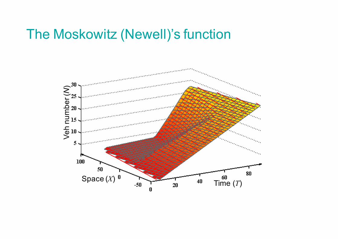
The Moskowitz (Newell)’s function

q = ∂t N

k = −∂xN

Space (X) Time (T)

Veh

num

ber (

N)

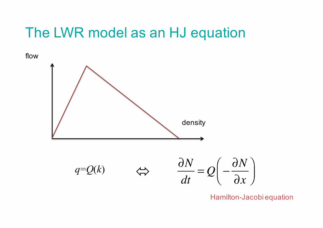
The LWR model as an HJ equationflow

density

q=Q(k) ∂Ndt

=Q − ∂N∂x

⎛⎝⎜

⎞⎠⎟ó

Hamilton-Jacobi equation

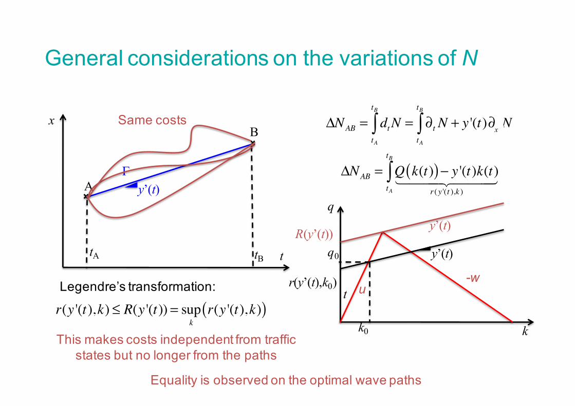
General considerations on the variations of N

y’(t)

tA tB

ΓA

Bx

ΔNAB = dtNtA

tB

∫ = ∂t N + y '(t)∂n NtA

tB

∫

ΔNAB = Q k(t)( )− y '(t)k(t)r (y '(t ),k )

tA

tB

∫

t

k

q

k0

q0 y’(t)

r(y’(t),k0) -wu

Same costs

Legendre’s transformation:

r(y '(t),k) ≤ R(y '(t)) = supk

r(y '(t),k)( )

y’(t)R(y’(t))

This makes costs independent from traffic states but no longer from the paths

Equality is observed on the optimal wave paths

t

x

APPLICATIONS TO SCALING-UP PROBLEMS (1)

13

Mean traffic behavior on urban corridors

Traffic dynamics at an isolated signal (1)

k

q

κkc

A

B

C

O

(a1)

(a2)

A

A

A

B

A

CO

t

xrouge vert

OA

B

C

s

v

ρ sc

(b1)

(b2)

A

A A

CB

A

0 0

t

n

n0

x

rouge vert

k

q

κkc

A

B

C

O

(a1)

(a2)

A

A

A

B

A

CO

t

xrouge vert

OA

B

C

s

v

ρ sc

(b1)

(b2)

A

A A

CB

A

0 0

t

n

n0

x

rouge vert

Fundamental Diagram (FD)

Full description of traffic dynamics

Traffic dynamics at an isolated signal (2)k

q

κkc

A

B

C

O

(a1)

(a2)

A

A

A

B

A

CO

t

xred green

k

q

κ’κ

A

A’

B’C

FD FD’

(b1)

(b2)

A

A A’ A

A

B’

AA’A

C

t

x

FD’

FD

k

q

κkc

A

B

C

O

(a1)

(a2)

A

A

A

B

A

CO

t

xred green

k

q

κ’κ

A

A’

B’C

FD FD’

(b1)

(b2)

A

A A’ A

A

B’

AA’A

C

t

x

FD’

FD

k

q

κkc

A

B

C

O

(a1)

(a2)

A

A

A

B

A

CO

t

xrouge vert

OA

B

C

s

v

ρ sc

(b1)

(b2)

A

A A

CB

A

0 0

t

n

n0

x

rouge vert

Input flows

Mean traffic states

Flow

Density

Local FD

Link Capacity

MFD

Estimating mean traffic states on corridor

• Definitions– corridor: series of m successive links ended by traffic

signals– Homogeneous traffic conditions, i.e. no or well-

balanced turning flow– FD parameters: free-flow u, wave speed w, jam

density κ

hyperlinklink i

GiCiδi

MFD ?

Traffic dynamics for an urban corridor

Intersections becomes correlatedA new phenomenon can be observed : spillbacks

Analytical Method (1) – Cuts for a corridor

t

x

hype

rlink

Flow

Density or accumulation

(Daganzo and Geroliminis, 2008)

Copy

Copy

Moving observer (mean speed V)V

Minimum overtaking flow R(V)R(V)

Cut: Q=minV(KV+R(V))

V

R(V)

MFD

Calculating R(V) with VT

t

x

Time window Tj(Vk)

B

A

Vku

To minimize costs, the observer has to maximize the time spent on red phases – Shortcuts theory (Daganzo and Menendez, 2005)Internal subpaths with v<u may be replaced at same costs.

A graph can simply be constructed to explore all the possible paths

Analytical Method (2) - The sufficient graph

The cost R(V) for different V can be calculated using a sufficient graph defined by three kinds of edges:

• edge (a): red phase (cost 0)• edge (b): green phase (cost Qmax)• edge (c): path with speed u or -w that starts at the end of red phases (cost 0 or wκ)

A

Vj>0

B

(c)

t

x

edge (a) edge (b) edge (c)

Vj

Cut

NFD

Rj

(a)

K (or N)

QMoving observer path

Vj>0

Vj<0

urba

n co

rrido

r

green phase red phase

(b)

t

x

link i

(Leclercq and Geroliminis, 2013)

The estimation is tight only if the network is homegenously

loaded

Influence of the time lag between signals

0 20 40 60 80 100 120 140 160 1800

200

400

600

800

1000

1200

1400

1600

1800

Density [veh/km]

Flow

[Veh

/h]

0 20 40 60 80 100 120 140 160 1800

200

400

600

800

1000

1200

1400

1600

1800

Density [veh/km]

Flow

[Veh

/h]

0 20 40 60 80 100 120 140 160 1800

200

400

600

800

1000

1200

1400

1600

1800

Density [veh/km]

Flow

[Veh

/h]

0 20 40 60 80 100 120 140 160 1800

200

400

600

800

1000

1200

1400

1600

1800

Density [veh/km]

Flow

[Veh

/h]

0 20 40 60 80 100 120 140 160 1800

200

400

600

800

1000

1200

1400

1600

1800

Density [veh/km]

Flow

[Veh

/h]

0 20 40 60 80 100 120 140 160 1800

200

400

600

800

1000

1200

1400

1600

1800

Density [veh/km]

Flow

[Veh

/h]

0 20 40 60 80 100 120 140 160 1800

200

400

600

800

1000

1200

1400

1600

1800

Density [veh/km]

Flow

[Veh

/h]

0 20 40 60 80 100 120 140 160 1800

200

400

600

800

1000

1200

1400

1600

1800

Density [veh/km]

Flow

[Veh

/h]

δ=0 s δ=10 s δ=20 s δ=30 s δ=40 s δ=50 s δ=60 s δ=70 s 0 20 40 60 80 100 120 140 160 180

0

200

400

600

800

1000

1200

1400

1600

1800

Density [veh/km]

Flow

[Veh

/h]

APPLICATIONS TO SCALING-UP PROBLEMS (2)

22

Capacity drop at freeway merges

Hypothesis

• Network:– The main road has only one lane– The inserting flow is equal to q0– LWR model and triangular fundamental diagram

(free-flow speed u wave speed w and jam density κ)• Insertions:

– Time between two insertions: H(h0=1/q0, sH)– Inserting positions are uniformly distributed between 0 and L– Vehicles insert at speed v0 with an acceleration a and a jam

density κ– Inserting vehicles behave as moving bottlenecks on target lane

23

(a)xi

L

x=0 x=L

i

t

x(b)

v0,iti ti+1

τ(hi,ai,v0,i)

hi

A B

C

void

A BC

D D’

t

x(c)

t1 t2 t3 t4 t5 t6 t7 t8 t9

t’0 t’2 t’1 t’3 t’5 t’4 t’8t*0 t*1 t*2 t*3 t*4 t*5 t*6

h’1

L

x1

(d)

v1, k

v1, k

v1, l

v1, l

v0

v0A

B C

t

x

xT

xT’ k

l

i

T T’

t’k t’lt’i t’lh’i ∆h’i

hi

hk

q0

Case 1: L=0 and sH>0

24

t

x

t

x

tt

x

ti ti+1

hi

tt

x

ti ti+1

τ(hi)

hi

A BC

w

t

C N N h ni ii

n

ii

n

! �" # � $�$! !� �1

1 1

/ with

The effective capacity C is given by :

Simplest homogeneous case(L=0, sH>0)

• Effective capacity

• Law of large numbers

• Second order Taylor approximation

( / ) ( ) ( / ) ( ) ( )1 11

n h E h n h E hi ii

n

i ii

� � ! "# #� and � �

11

n

�

E h E h sh

E h h as wi i

ii� �

��( ) ( )! " ! "! " # �

�! " $ ! " ��

12

22

2 0

2 22

02

0

3 22 2w v awh#! " #! " /

t

x

ti ti+1

τ(hi)

hi

A BC

w

t

C w h h h w vi

i

n

ii

n

i! ��

��

�! �

"

! !� �� � �1

1 1

( ) / ( ) and 000

21 2a a

w v awhi" " "( )

∑ ∑κ τ( )( )= −= =

C w h h h/i ii

n

ii

n

1 1

C w h h h w vi

i

n

ii

n

i! ��

��

�! �

"

! !� �� � �1

1 1

( ) / ( ) and 000

21 2a a

w v awhi" " "( )

25(Leclercq et al, part B, 2011)

Case 2: L>0 and sH>0 – no interactions

26

t

x t1 t2 t3 t4 t5 t6 t7 t8 t9

L

h0

t

x t1 t2 t3 t4 t5 t6 t7 t8 t9

L

h0

t

x t1 t2 t3 t4 t5 t6 t7 t8 t9

t’0 t’2 t’1 t’3 t’5 t’4 t’8

L

h0

t

x t1 t2 t3 t4 t5 t6 t7 t8 t9

t’0 t’2 t’1 t’3 t’5 t’4 t’8t’(0) t’(1) t’(2)t’(3) t’(4) t’(5) t’(6)

L

h0

A BC

D

t

x t1 t2 t3 t4 t5 t6 t7 t8 t9

t’0 t’2 t’1 t’3 t’5 t’4 t’8t’(0) t’(1) t’(2)t’(3) t’(4) t’(5) t’(6)

L

h0

A BC

DD’

t

x t1 t2 t3 t4 t5 t6 t7 t8 t9

t’0 t’2 t’1 t’3 t’5 t’4 t’8t’(0) t’(1) t’(2)t’(3) t’(4) t’(5) t’(6)

L

h0

A BC

DD’

t

x t1 t2 t3 t4 t5 t6 t7 t8 t9

t’0 t’2 t’1 t’3 t’5 t’4 t’8t’(0) t’(1) t’(2)t’(3) t’(4) t’(5) t’(6)

h’1

L

h0

Same problem as case 1 by switching inserting times and t’() at x=0 !

Resulting analytical curves

q0=0.174 veh/s

q0=0.08 veh/s

q0=0.26 veh/s

0 50 100 150 200 250 3000.2

0.25

0.3

0.35

0.4

L [m]

C [veh/s] (a)

0 50 100 150 200 250 3000.2

0.25

0.3

0.35

0.4

(b)

L [m]

C [veh/s]

NumericalAnalytical

0 50 100 150 200 250 3000.2

0.25

0.3

0.35

0.4

L [m]

C [veh/s] (c)

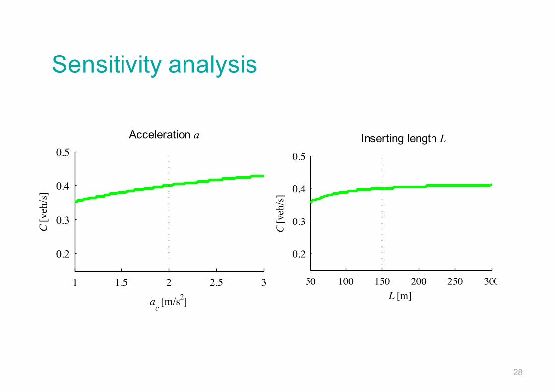
28

Sensitivity analysis

50 100 150 200 250 300

0.2

0.3

0.4

0.5(a)

L [m]C

[veh

/s]

50 100 150 200 250 300

0.2

0.3

0.4

0.5(b)

LDLC [m]

C [v

eh/s

]

0.5 1 1.5

0.2

0.3

0.4

0.5(c)

αl

C [v

eh/s

]

1 1.5 2 2.5 3

0.2

0.3

0.4

0.5(d)

ac [m/s2]

C [v

eh/s

]

1 1.5 2 2.5 3

0.2

0.3

0.4

0.5(e)

at [m/s2]

C [v

eh/s

]1 2 3 4 5

0.2

0.3

0.4

0.5(f)

τ [s]

C [v

eh/s

]

0 0.5 1

0.2

0.3

0.4

0.5(g)

p [%]

C [v

eh/s

]

Inserting length L

50 100 150 200 250 300

0.2

0.3

0.4

0.5(a)

L [m]

C [v

eh/s

]

50 100 150 200 250 300

0.2

0.3

0.4

0.5(b)

LDLC [m]

C [v

eh/s

]

0.5 1 1.5

0.2

0.3

0.4

0.5(c)

αl

C [v

eh/s

]

1 1.5 2 2.5 3

0.2

0.3

0.4

0.5(d)

ac [m/s2]

C [v

eh/s

]

1 1.5 2 2.5 3

0.2

0.3

0.4

0.5(e)

at [m/s2]

C [v

eh/s

]

1 2 3 4 5

0.2

0.3

0.4

0.5(f)

τ [s]

C [v

eh/s

]

0 0.5 1

0.2

0.3

0.4

0.5(g)

p [%]

C [v

eh/s

]

Acceleration a

Extended framework

• Refined description of traffic dynamics (interactions between waves and voids)(Leclercq, Knoop et al, part C, in press)

• Heterogeneous vehicle characteristics(Leclercq et al, part C, in press)

• Multilane on freeways(Leclercq et al, TRB2016)

(a)xi

L

x=0 x=L

i

t

x(b)

v0,iti ti+1

τ(hi,ai,v0,i)

hi

A B

C

void

A BC

D D’

t

x(c)

t1 t2 t3 t4 t5 t6 t7 t8 t9

t’0 t’2 t’1 t’3 t’5 t’4 t’8t*0 t*1 t*2 t*3 t*4 t*5 t*6

h’1

L

x1

(d)

v1, k

v1, k

v1, l

v1, l

v0

v0A

B C

t

x

xT

xT’ k

l

i

T T’

t’k t’lt’i t’lh’i ∆h’i

hi

hk

(a)xi

L

x=0 x=L

i

t

x(b)

v0,iti ti+1

τ(hi,ai,v0,i)

hi

A B

C

void

A BC

D D’

t

x(c)

t1 t2 t3 t4 t5 t6 t7 t8 t9

t’0 t’2 t’1 t’3 t’5 t’4 t’8t*0 t*1 t*2 t*3 t*4 t*5 t*6

h’1

L

x1

(d)

v1, k

v1, k

v1, l

v1, l

v0

v0A

B C

t

x

xT

xT’ k

l

i

T T’

t’k t’lt’i t’lh’i ∆h’i

hi

hk

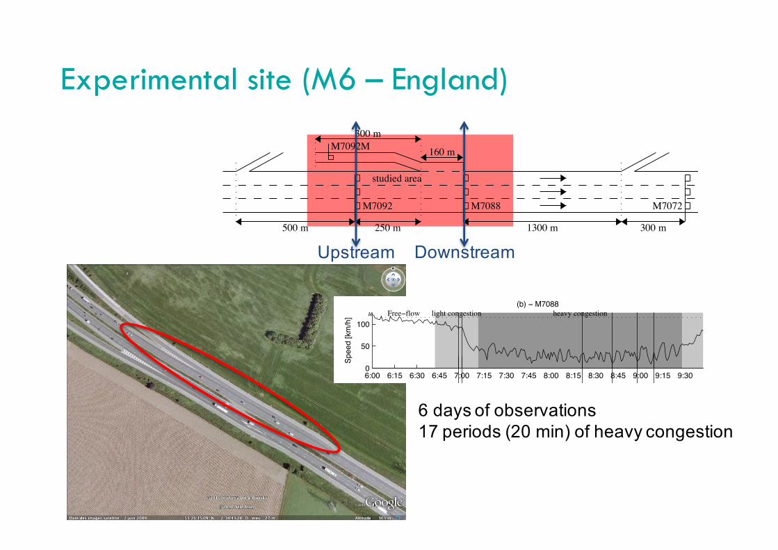
Experimental site (M6 – England)

studied area

M7072M7092 M7088

M7092M

500 m 250 m

160 m

1300 m 300 m

300 m

6:00 6:15 6:30 6:45 7:00 7:15 7:30 7:45 8:00 8:15 8:30 8:45 9:00 9:15 9:300

50

100Free−flow light congestion heavy congestionu

Spee

d [k

m/h

]

6:00 6:15 6:30 6:45 7:00 7:15 7:30 7:45 8:00 8:15 8:30 8:45 9:00 9:15 9:300

2000

4000

6000 M7088

M7092

Flow

[veh

/h]

C B1

B2

A1

A2

6:00 6:15 6:30 6:45 7:00 7:15 7:30 7:45 8:00 8:15 8:30 8:45 9:00 9:15 9:300

1000

2000

Flow

[veh

/h]

lane 1lane 2lane 3

Upstream Downstreamstudied area

M7072M7092 M7088

M7092M

500 m 250 m

160 m

1300 m 300 m

300 m(a)

6:00 6:15 6:30 6:45 7:00 7:15 7:30 7:45 8:00 8:15 8:30 8:45 9:00 9:15 9:300

50

100Free−flow light congestion heavy congestionu

Spee

d [k

m/h

]

(b) − M7088

6:00 6:15 6:30 6:45 7:00 7:15 7:30 7:45 8:00 8:15 8:30 8:45 9:00 9:15 9:300

2000

4000

6000 M7088

M7092

Flow

[veh

/h]

(c) − M7092 and M7088

C B1

B2

A1

A2

6:00 6:15 6:30 6:45 7:00 7:15 7:30 7:45 8:00 8:15 8:30 8:45 9:00 9:15 9:300

1000

2000

Flow

[veh

/h]

(d) − M7088

lane 1lane 2lane 3

6 days of observations17 periods (20 min) of heavy congestion

Extended sketch of the modelstudied area

M7072M7092 M7088

M7092M

500 m 250 m

160 m

1300 m 300 m

300 m(a)

(b)

Lane 1

Lane 2

Lane 3

C1

C2

C3

q1

q2

q3

LL1DLCL2

DLC

q0

q12

q23

q1 + q12

q2 + q23

Merge 1Merge 2Merge 3

0 200 400 600 800 1000 12000

500

1000

αl = 1.39

q1 [veh/h]

q 0 [veh

/h]

(c)

0 500 1000 1500 2000 25000

500

1000

1500

2000

p = 1

C2 [veh/h]

C 3 [veh

/h]

(d)

0 1000 2000 3000 4000 5000 6000 70000

500

1000

αg = 0.2

[

]

[ ]

q1 + q2 + q3 [veh/h]

q 0 [veh

/h]

(e)

ObservationsMean observationAnalytical predictions (Leclercq et al., 2011)Analytical prediction (no relaxation)Sensibility domain

L2DLC=L1

DLC

τ1=τ2

Rough calibration:

-FD (per lane): u=115 km/h, w=20 km/h, κ=145 veh/km -a=1.8 m/s2; τ1=τ2=3 s;-L=160 m ; L2

DLC=L1DLC=100 m

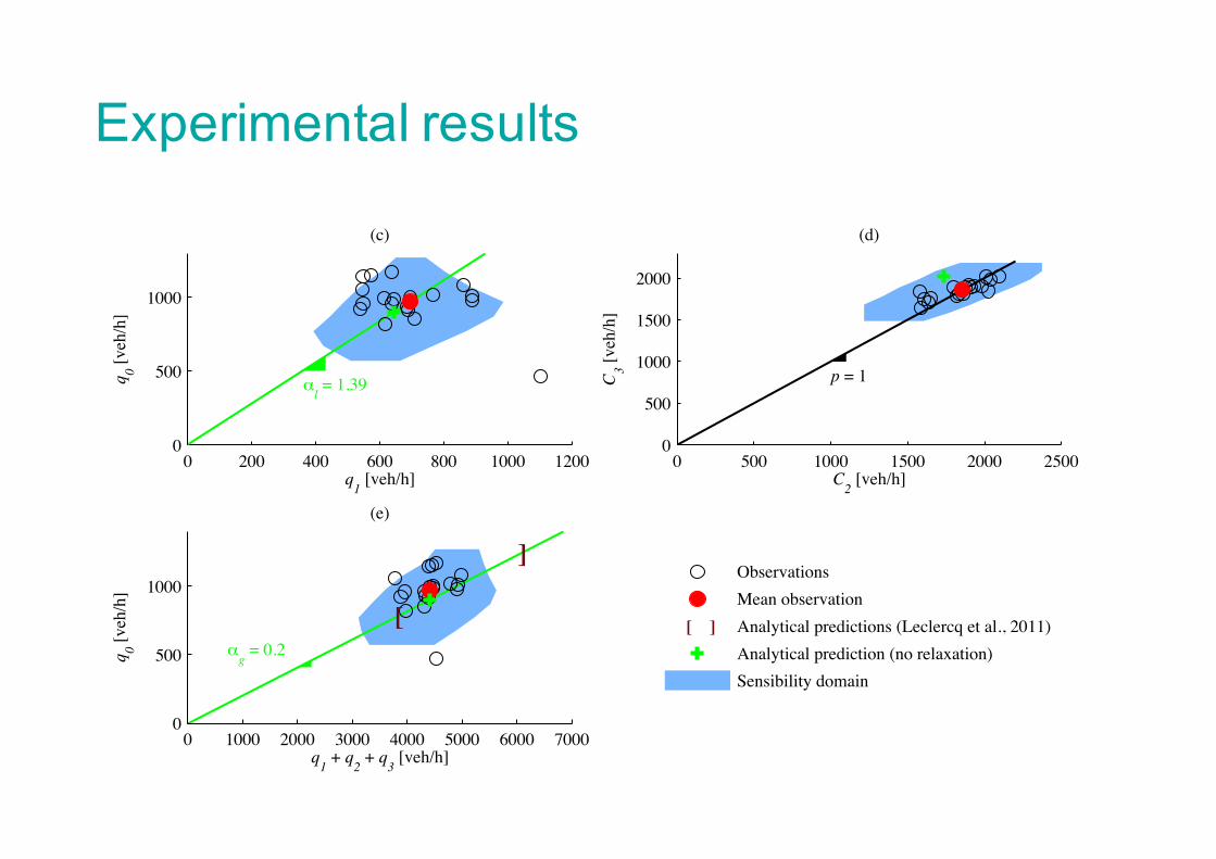
Experimental results

studied area

M7072M7092 M7088

M7092M

500 m 250 m

160 m

1300 m 300 m

300 m(a)

(b)

Lane 1

Lane 2

Lane 3

C1

C2

C3

q1

q2

q3

LL1DLCL2

DLC

q0

q12

q23

q1 + q12

q2 + q23

Merge 1Merge 2Merge 3

0 200 400 600 800 1000 12000

500

1000

αl = 1.39

q1 [veh/h]

q 0 [veh

/h]

(c)

0 500 1000 1500 2000 25000

500

1000

1500

2000

p = 1

C2 [veh/h]

C 3 [veh

/h]

(d)

0 1000 2000 3000 4000 5000 6000 70000

500

1000

αg = 0.2

[

]

[ ]

q1 + q2 + q3 [veh/h]

q 0 [veh

/h]

(e)

ObservationsMean observationAnalytical predictions (Leclercq et al., 2011)Analytical prediction (no relaxation)Sensibility domain

CONCLUSION

33

Conclusion

• Variational theory is a powerful to determine mean traffic states from a microscopic description of the physical mechanisms

• Variational theory is by nature an integrating operator

• A real challenge is to operate micro to macro transformations for transitional phases

• Consistent integration is very important for hierarchical modeling and to adress large scale problems

34

Thank you for your attention

35

Are you interested in collaborating on an very exiting project ?......

36

MAGnUM: A Multiscale and Multimodal Traffic Modelling Approach for Sustainable Management of Urban Mobility

RESIDUALS

37

Variational theory (VT) in Eulerian –General basis

q =Q(k) ⇔ ∂t k =Q −∂x k( )HJ Equation:

t

y’(t)

tO(Γ) tP

ΓO(Γ)

Px Ψ

NP = minΓ∈DP

NO Γ( ) + Δ Γ( )( )Δ Γ( ) = r(y '(t),k)dt

tO Γ( )

tP∫General expression for the solutions:

NP = minΓ∈DP

NO Γ( ) + Δ ' Γ( )( )Δ ' Γ( ) = R(y '(t))dt

tO Γ( )

tP∫

Key VT result usingthe Legendre’s transformation

VT is really useful with PWL FD(and especially triangular one)

VT in Eulerian – The Highway ProblemLi

nkx

t

N(x,t)

u

-w

N(xu,t-(x-xu)/u)

+0

N(xd,t-(xd-x)/w)

+κ(xd-x)

N (x,t) = min N xu ,t −(x − xu )

u⎛⎝⎜

⎞⎠⎟

free− flow

, N xd ,t −(xd − x)

w⎛⎝⎜

⎞⎠⎟+κ (xd − x)

congestion

⎡

⎣

⎢⎢⎢⎢

⎤

⎦

⎥⎥⎥⎥

Newell’s model (1993) !!!

Triangular FD