From Micro to Macro: Uncovering and PredictingInformation Cascading Process with Behavioral Dynamics

Linyun Yu1, Peng Cui1, Fei Wang2, Chaoming Song3, Shiqiang Yang1

1Department of Computer Science and Technology, Tsinghua University2Department of Computer Science and Engineering, University of Connecticut

3Department of Physics, University of Miamiyuly12@mails.tsinghua.edu.cn,cuip@tsinghua.edu.cn,fei_wang@uconn.edu

chaoming.song@gmail.com, yangshq@tsinghua.edu.cn

ABSTRACTCascades are ubiquitous in various network environments.How to predict these cascades is highly nontrivial in severalvital applications, such as viral marketing, epidemic preven-tion and traffic management. Most previous works mainlyfocus on predicting the final cascade sizes. As cascades aretypical dynamic processes, it is always interesting and im-portant to predict the cascade size at any time, or predictthe time when a cascade will reach a certain size (e.g. anthreshold for outbreak). In this paper, we unify all thesetasks into a fundamental problem: cascading process predic-tion. That is, given the early stage of a cascade, how to pre-dict its cumulative cascade size of any later time? For sucha challenging problem, how to understand the micro mech-anism that drives and generates the macro phenomenons(i.e. cascading proceese) is essential. Here we introduce be-havioral dynamics as the micro mechanism to describe thedynamic process of a node’s neighbors get infected by a cas-cade after this node get infected (i.e. one-hop subcascades).Through data-driven analysis, we find out the common prin-ciples and patterns lying in behavioral dynamics and proposea novel Networked Weibull Regression model for behavioraldynamics modeling. After that we propose a novel methodfor predicting cascading processes by effectively aggregat-ing behavioral dynamics, and propose a scalable solution toapproximate the cascading process with a theoretical guar-antee. We extensively evaluate the proposed method on alarge scale social network dataset. The results demonstratethat the proposed method can significantly outperform otherstate-of-the-art baselines in multiple tasks including cascadesize prediction, outbreak time prediction and cascading pro-cess prediction.

KeywordsInformation Cascades, Social Network, Dynamic ProcessesPrediction

Permission to make digital or hard copies of all or part of this work forpersonal or classroom use is granted without fee provided that copies arenot made or distributed for profit or commercial advantage and that copiesbear this notice and the full citation on the first page. To copy otherwise, torepublish, to post on servers or to redistribute to lists, requires prior specificpermission and/or a fee.Copyright 20XX ACM X-XXXXX-XX-X/XX/XX ...$15.00.

1. INTRODUCTIONIn a network environment, if decentralized nodes act on

the basis of how their neighbors act at earlier time, theselocal actions often lead to interesting macro dynamics - cas-cades. In online social networks, the information a usercan get and engage in is highly dependent on what his/herfriends share, and thus information cascades naturally occurand become the major mechanism for information commu-nication. There has been a growing body of research onthese information cascades because of their big potential invarious vital applications such as viral marketing, epidemicprevention, and traffic management. Most of them focus oncharacterizing these information cascades and discoveringtheir patterns in structures, contents and temporal dynam-ics.

Recently, predictive modeling on information cascades hasaroused considerable research interests. Earlier works onpredicting the final size of information cascades based oncontent, behavioral and structural features [3, 6]. As onlylarge cascades are of interest in most real applications, Cui etal.[6] propose a data driven approach to predicting whetherthe final size will surpass a threshold for outbreak. Morerecently, Cheng et al.[3] go beyond the final size to contin-uously predict whether the cascade will double the currentsize in future. They also raise an interesting question thatwhether cascades can be predicted, and their experimentalresults demonstrate that cascade size are highly predictable.However, the previous works were all about cascade size,which did not include the whole of information cascades.Information cascade is a typical dynamic process, and tem-poral scale is critical for understanding the cascading mech-anism. Also, it is highly nontrivial to predict when a cascadebreaks out, and, more ambitiously, to predict the evolvingprocess of a cascade (i.e. cascading process, as shown in 1(a)). In this paper, we move one step forward to ask: Isthe cascading process predictable? That is, given the earlystage of an information cascade, can we predict its cumula-tive cascade size of any later time?

It is apparent that the targeted problem is far more chal-lenging than those in previous works. The commonly usedcascade-level macro features for size prediction, such as thecontent, increasing speed and structures in the early stageare not distinctive and predictive enough for the cascadesizes at any later time. A fundamental way to address thisproblem is to look into the micro mechanism of cascadingprocesses. Intuitively, an information cascading process canbe decomposed into multiple local (one-hop) subcascades.

arX

iv:1

505.

0719

3v1

[cs

.SI]

27

May

201

5

Predictedcascading process

Earlystage

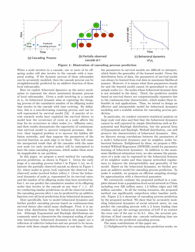
(a) Cascading Process (c) Behavioral dynamicsof 𝑝1

(b) Partially observed cascade at t

Figure 1: Illustration of cascading process prediction

When a node involves in a cascade, one or more of its off-spring nodes will also involve in the cascade with a tem-poral scaling. If the dynamic process of these subcasadescan be accurately modeled, then the cascade process can bestraightforwardly predicted by an additive function of theselocal subcascades.

Here we exploit behavioral dynamics as the micro mech-anism to represent the above mentioned dynamic processof local subcascades. Given a node involving in a cascadeat t0, its behavioral dynamic aims at capturing the chang-ing process of the cumulative number of its offspring nodesthat involve in the cascade with time evolving. By defini-tion, this is a non-decreasing counting process and can bewell represented by survival model [16]. A paucity of re-cent research works have exploited the survival theory tomodel how the occurrence of event at a node affects thetime for its occurrence at other nodes (i.e. diffusion rate),and their results demonstrate the superiority of continuous-time survival model to uncover temporal processes. How-ever, their targeted problem is to uncover the hidden dif-fusion networks, and thus suppose the parameters of thesurvival function on each edge to be fixed. This will causethe unexpected result that all the cascades with the sameroot node (or early involved nodes) will be anticipated tohave the same cascading processes, which makes these mod-els inapplicable in our problem.

In this paper, we propose a novel method for cascadingprocess prediction, as shown in Figure 1. Given the earlystage of a cascading process before t in Figure 1 (a), we il-lustrate the partially observed cascade as shown in Figure 1(b), where nodes in green (red) represent the observed (un-observed) nodes involved before (after) t. Given the behav-ioral dynamics of node p1 represented by its survival rates,and the number of its offspring nodes that have involved be-fore t, we can predict the cumulative number of its offspringnodes that involve in the cascade at any time t′ > t. Af-ter conducting similar predictions on all the observed nodes,the cascading process after t can be predicted by an additivefunction over all local predictions from behavioral dynamics.

More specifically, how to model behavioral dynamics andfurther predict cascading process based on continuous-timesurvival theory also entail many challenges. First, it is un-clear what distribution form the behavioral dynamics fol-low. Although Exponential and Rayleigh distributions arecommonly used to characterize the temporal scaling of pair-wise interactions, behavioral dynamics in this paper are areflection of collective behaviors and are proved to be incon-sistent with these simple distributions in real data. Second,

the parameters in survival models are difficult to interpret,which limits the generality of the learned model. Given thedistribution form of data, the parameters of survival modelcan always be learned from real data in maximum likelihoodmanner. However, it is unsure what these parameters standsfor and the learned model cannot be generalized to out-of-sample nodes (i.e. the nodes whose behavioral dynamic datais not included in the data). Third, the predictive modelsbased on survival theory are computationally expensive dueto the continuous-time characteristic, which makes them in-feasible in real applications. Thus, we intend to design aneffective and interpretable model for behavioral dynamicsmodeling and a scalable solution for cascading process pre-diction.

In particular, we conduct extensive statistical analysis onlarge scale real data and find that the behavioral dynamicscannot be well captured by simple distributions such as Ex-ponential and Rayleigh distribution, but the general formof Exponential and Rayleigh, Weibull distribution, can wellpreserve the characteristics of behavioral dynamics. Also,we discover strong correlations between the parameters ofa node’s behavioral dynamics and its neighbor nodes be-havioral features. Enlightened by these, we propose a NEt-worked WEibull Regression (NEWER) model for parameterlearning of behavioral dynamics. In addition to the maxi-mum likelihood estimation term, we also assume the param-eters of a node can be regressed by the behavioral featuresof its neighbor nodes and thus impose networked regular-izers to improve the interpretability and generality of themodel. Based on the behavioral dynamics, we further pro-pose an additive model for cascading process prediction. Tomake it scalable, we propose an efficient sampling strategyfor approximation with a theoretical guarantee.

We extensively evaluate the proposed method in a com-plete dataset from a population-level social network in China,including over 320 million users, 1.2 billion edges and 340million cascades . In all the testing scenarios, the proposedmethod can significantly outperform other baseline meth-ods. Figure 2 is a showcase of cascading process predictionby the proposed method. We show that by accurately mod-eling behavioral dynamics of social network users, we canpredict the cascading process with a 2 hours leading timewindow, and get the average precision of 0.97 if we restrictthe error rate of the size to be 0.1. Also, the accurate pre-dictions of final cascade size, cascade outbreaking time areall implied in the predicted cascading process.

The main contributions of this paper are:(1) Enlightened by the cascading size prediction works, we

Esp = 0.1

Early stage Percentage=0.2

Early stage Percentage=0.3

Early stage Percentage=0.5

δ0.2-Precision=0.52

δ0.2-Precision=0.63

δ0.2-Precision=0.85

δ0.2-Precision=0.94

Figure 2: Showcase of cascading process predic-tion for a real cascade. The red line represents thegroundtruth cascading process. The others are pre-diction results based on different early stage infor-mation.

move one step forward to attempt cascading process predic-tion problem, which implies several vital problems such ascascade size prediction, outbreaking time prediction as wellas evolving process prediction.

(2) We find out the common principles and patterns ly-ing in behavioral dynamics and propose a novel NetworkedWeibull Regression model for behavioral dynamics modelingaccordingly, which significantly improves the interpretabilityand generality of traditional survival models.

(3) We propose a novel method for predicting macro cas-cading process by aggregating micro behavioral dynamics,and propose a scalable solution to approximate the cascad-ing process with a theoretical guarantee.

2. RELATED WORKPrediction on Cascades. In recent years, many methodshave been proposed to make prediction on cascades. Mostof them focus on predicting the future size of a cascade, andthe common way is to select vital nodes and place sensors onthem. For example, Cohen et al. [4] focus on exploring thetopological characteristics of the cascade. Cui et al. [6] pro-poses to optimize the size prediction problem using dynamicinformation. Cheng et al. [3] introduces temporal featureinto the problem and they predict the growing size of thecascade. Rather than attempt to predict the cascade size,we focus on predicting the cascading process which considersboth time and volume information together.Survival Model. Survival model is a method try to anal-ysis things according to the time duration until one or moreevents happen. In recent years, researchers started model-ing information diffusion using continuous models. Myerset al. [14] proposed CONNIE to infer the diffusion networkbase on convex programming while leaving the transmissionrate to be fixed, later on Rodriguez et al.[17] proposed NE-TRATE which allowing the transmission rate to be differentin different edges. Subsequently, Rodriguez et al. [10] givean additive model and a multiplicative model to describeinformation propagation base on survival theory. Most ofthese works focus on discovering the rules and patterns tothe edges in the social network and is hard to extend tomake predictions for cascades since the correlation betweentransmission rates on edges is little. In contrast, our workfocus more on predictive modeling by grouping correlatededges together so that we can make predictions for edges

base on the information of other edges.Influence Modeling and Maximization. Influence mod-eling and maximization aims to evaluate users’ importancein social networks. This is first proposed by Domingos et al.[7] to select early starters to trigger a large cascade. ThenKempe et al. [12] proposed Stochastic Cascade Model to for-malize the problem and Chen et al. [2] proposed a scalablesolutions. Recently the approach was extended to addingopinion effect [1, 9] or time decay effects [18] on the models.Our work is distinct from existing works in the followingway: Rather than quantify the influence on nodes, we willpredict the cascading process.

3. PRELIMINARIESThis section presents the dataset information, discovered

patterns and validated hypothesises to support the modeldesign and solution.

3.1 Dataset DescriptionThe dataset in this paper is from Tencent Weibo, one of

the largest Twitter-style websites in China. We collect allthe cascades in 10 days generated between Nov 15th andNov 25th in 2011. The dataset contains in total 320 mil-lion users with their social relations, 340 million cascades1

with their explicit cascading processes. The distribution ofcascade size is shown in Figure 3. We can see that the cas-cade size follows Power-Law distribution, and the majorityof cascades have very small size, which are not of interest formany applications. As the paper intends to predict cascad-ing process, we filter out the cascades with the size of lessthan 5, and maintain the remaining 0.59 million cascadeswith obvious cascading process for statistical analysis andexperiments.

`

y=-1.66x+5.92

Figure 3: Distribution of cascade size. The redstraight line is the linear fitting result to the bluecurve, showing the size distribution fits power-law.

3.2 Characteristics of Behavioral DynamicsAs mentioned before, behavioral dynamics play a central

role in uncovering and predicting cascade processes. Here weinvestigate the characteristics of behavioral dynamics to en-lighten the modeling of behavioral dynamics. By definition,the behavioral dynamics of a user capture the changing pro-cess of the cumulative number of his/her followers retweet

1Here the cascades are information cascades. When a userretweet/generate a post, several of his/her followers will fur-ther retweet the post and so on so forth to form a informationcascade.

model density function survival function hazard function ks-static in Weibo

Exponential λie−λit e−λit λi 0.2741

Power Law αiδ

(tδ

)−αi−1 (tδ

)−αi αit

0.9893

Rayleigh αite−αi t

2

2 e−αit2

2 αit 0.7842

Weibull kiλi

(tλi

)ki−1

e−(tλi

)kie−(tλi

)kikiλi

(tλi

)ki−1

0.0738

Table 1: Parametric Models

a post after the user retweeting the post. Then the behav-ioral dynamics of a user can be straightforwardly representedby averaging the size growth curve of all subcascades thatspread to the user and his/her followers. However, Figure 4shows that the size growth curves vary significantly for dif-ferent subcascades of the same user, which means that sucha representation is not fit to characterize behavioral dynam-ics. Here we normalize the size growth process by the cas-cade final size and adopt survival function to describe thebehavioral dynamics where the survival rate represents thepercentage of nodes that has not been but will be infected.As shown in Figure 4, a user’s survival function is quitestable for different subcascades although their size growthpatterns vary.

Figure 4: The size growth curves and their corre-sponding survival function for 3 users.

Then can we use the behavioral dynamics represented bysurvival function to predict the size growth curve of a sub-cascade? We provide positive answer with the assistanceof early stage information. For example, if we know thesubcascade size at an early time t0, then the survival func-tion can be straightforwardly transformed from percentagedimension into size dimension.

3.3 Parametrize Behavioral DynamicsFor the ease of computation and modeling, we need to

parametrize the behavioral dynamics in our case. In state-of-the-art, Exponential and Rayleigh distributions are oftenused to describe the dynamics of user behaviors in differentsettings [8, 11]. Here we testify these distribution hypothesison our real data and find that these distributions cannot wellcapture both the shape and scale characteristics of behav-ioral dynamics. Thus, we turn to the general form of Expo-nential and Rayleigh distributions, the Weibull distribution[15], and find it adequate for parametrizing behavioral dy-namics. In order to quantify the effect of parametrization,we calculate KS-Statistic for the three candidate distribu-tions as shown in Table 1. It displays that Weibull distribu-tion performs much better than Exponential and Rayleighdistribution. The improvement is attributed to the highdegree of freedom of Weibull distribution as it has two pa-rameters λ and k to respectively control the scale and shapeof the behavioral dynamics.

3.4 Covariates of Behavioral DynamicsIf subcascades for all users are sufficient, the parameters

of behavioral dynamics can be directly learned from data.

Behavioral featuresinflow rate the number of the posts user re-

ceived in a certain period.outflow rate the number of the posts user sent

in a certain period.average inflow rate of fans to the

follower avg− user, or∑i retweet(i)·in flow(i)∑

i retweet(i)

inflow rate where i is the fans to the user(andthe same as following).

follower avg− average retweet rate of fans to the

retweet rate user, or∑i retweet(i)·retweet rate(i)∑

i retweet(i).

Structural featuresfollower number number of the followers to the user.follow number number of users this user follows.

Table 2: Behavioral features for users.

However this suffers from several drawbacks: (1) some usersmay have no or very sparse subcascade in training dataset,which makes these users’ behavioral dynamics inaccurateor even unknown; (2) it is difficult to interpret the param-eters directly learned from data, which prohibits us fromgetting insightful understanding on the behavioral dynam-ics. To address these, we investigate the covariates of be-havioral dynamics here. As the behavioral dynamics of auser are to capture the collective responses of his/her fol-lowers, we assume the parameters of the user’s behavioraldynamics should be correlated with the behavioral featuresof his/her followers (network neighbors). Hence, we extracta set of behavioral features for each user as listed in Table 2.2

For each user with enough subcascades in our dataset, welearned their λ and k directly from data. And then, we cal-culate the correlations between the learned parameters andtheir followers’ collective behavioral features. The examplesgiven in Figure 5 indicate obvious correlations between thelearned parameters with these behavioral features. There-fore, we can use these behavioral features as covariates toregress the parameters of behavioral dynamics.

3.5 From Behavioral Dynamics to CascadesAfter validating that the behavioral dynamics can poten-

tially be accurately modeled and predicted, the key problemis whether we can derive the macro cascading process frommicro behavioral dynamics. Intuitively, the cascading pro-cess cannot be perfectly predicted at early stage by behav-ioral dynamics. Given any time t, we can only use the behav-ioral dynamics of the users that involved before t to predictthe cascading process after t. Consequently, the predictioncoverage is restricted to all the followers of these users, whilethe users beyond this scope are neglected. These uncoveredusers may potentially affect the performance of cascadingprocess prediction.

2We think that follower with different retweet numberwill have different effects to the user, so we modify theweights on each term of follower avg inflow rate andfollower avg retweet rate.

Figure 5: Correlations between the survival functionparameters and the behavioral features

Fortunately, we observe two interesting phenomenons inreal data.

Minor dominance. Although each user has behavioraldynamics, the behavioral dynamics of different users makesignificantly different contributions to the cascading process.It is intuitive that the behavioral dynamics of an active userwith 1 million followers contribute much more than that ofan inactive user with 5 followers. The data also coincideswith our intuition. According to Figure 6 (a), it can beobserved that a very small number of nodes whose behav-ioral dynamics dominate the cascading process underpin theidea of just using the behavioral dynamics of these dominantnodes for cascading process prediction.

Early stage dominance. Enlightened by the minordominance phenomenon, we further ask whether the domi-nant nodes are prone to join cascades in early stage. Here,Figure 6 (b) depicts the time distribution of these dominantnodes joining in cascades,

Figure 6: Minor dominance and early stage domi-nance in information cascades.

Taking these two phenomena into account together, it issafe to design a model exploiting the behavioral dynamicsof infected nodes in early stage to predict the cascading pro-cess.

4. METHODOLOGYThis section introduces the NEtworked WEibull Regres-

sion (NEWER) and cascade prediction methods in detail.

4.1 Problem StatementGiven a network G = 〈U,A〉, where U is a collection of

nodes and A is the set of pairwise directed/undirected re-lationships. An event (e.g., tweet) can be originated from

one node and spread (e.g., by retweeting) to its neighbor-ing nodes. A cascade is typically formed by repeating thisprocess. Therefore, a cascade can be represented by a set ofnodes C = {u1, u2, ...um}, where u1 is the root node. In acascade, each node will get infected by the event only once,so it is tree-structured. For every node ui in the cascade, wedenote its parent node as rp(ui). The time stamp that uigets infected is t(ui), and t(ui) ≤ t(ui+1). Then the partialcascade before time t is denoted by Ct = {ui|t(ui) ≤ t}, andits size size(Ct) = |Ct| where |.| is the cardinality of a set.Then the cascade prediction problem can be defined as:

Cascade Prediction: Given the early stage of a cascadeCt, predict the cascade size size(Ct′) with t′ ≥ t.

4.2 Survival AnalysisSurvival analysis is a branch of statistics that deals with

analysis of time duration until one or more events happen,such as death in biological organisms and failure in mechan-ical systems [13]. It is a useful technique for cascade predic-tion. More concretely, let τ0 be a non-negative continuousrandom variable representing the waiting time until the oc-currence of an event with probability density funtion f(t),the survival function

S(t) = Pr{τ0 ≥ t} =

∫ ∞t

f(t) (1)

encodes the probability that the event occurs after t, thehazard rate is defined as the event rate at time t condi-tional on survival until time t or later (τ0 ≥ t), i.e.,

λ(t) = limdt→0

Pr(t ≤ τ0 < t+ dt|τ0 ≥ t)dt

=f(t)

S(t)(2)

S(t) and λ(t) are the two core quantities in survival anal-ysis.

4.3 NEtworked WEibull Regression ModelThe Weibull distribution is commonly used in survival

analysis.In network scenario, if we think the time that anevent (e.g., retweet) happened on a node as a survival pro-cess, we can fit a Weibull distribution to the survival time ofnode i, then its corresponding density, survival and hazardfunctions

fi(t) =kiλi

(t

λi

)ki−1

exp−(tλi

)ki(3)

Si(t) = exp−(tλi

)ki(4)

hi(t) =kiλi

(t

λi

)ki−1

(5)

where t > 0 is the average event happening time to node i,λi > 0 and ki > 0 is the scale and shape parameter of theWeibull distribution. In the following we will assume thenetwork nodes are users and the event is retweeting.

Likelihood of retweeting dynamics. Supposing thereare N users in total, Ti is a set of mi time stamps and eachelement Ti,j indicates the j-th retweet time stamp to thepost of the i-th user. We sort those time stamps out inincreasing order so that Ti,j+1 > Ti,j . We assume Ti,j ≥ 1and Ti,mi > 1. Then the likelihood of the event data can bewritten as follows:

L(λ, k) =

N∏i=1

mi∏j=1

(hi(Ti,j) · Si(Ti,j))

=

N∏i=1

mi∏j=1

(ki · T ki−1

i,j · λ−kii · e−Tkii,j ·λ

−kii

)(6)

logL(λ, k) =

N∑i=1

li(λi, ki) (7)

where li(λi, ki) = mi log ki + (ki − 1)∑mij=1 log Ti,j−

miki log λi − λ−kii

∑mij=1 T

kii,j .

As discovered in section 3.4, the survival characteristicsof the user is correlated with the behavioral features ofhim/her. Then we can parametrize those parameters inthe personalized Weibull distributions using those behav-ioral features. More formally, let xi be a r dimensional fea-ture vector for user i, we parameterize λi and ki with thefollowing linear function:

log λi = log xi ∗ β (8)

log ki = log xi ∗ γ (9)

where β and γ are r-dimensional parameter vector for λand k. We attempt to find the scale and shape parameterof every user so that the likelihood of the observed data ismaximized, at the same time we can also get the parametervectors for out-of-sample extensions.

We use the Equation (8) and (9) to replace λi and kiin the log likelihood function Equation (7) to solve the pa-rameters. To further enhance the interpretability, we alsoadd `1 sparsity regularizers on β and γ respectively to en-force model sparsity. Combining everything together, wecan obtain the NEtworked WEibull Regression (NEWER)formulation which aims to minimize the following objective:

F (λ, k, β, γ) = G1(λ, k) + µG2(β, λ) + ηG3(γ, k) (10)

G1(λ, k) = − logL(λ, k) (11)

G2(λ, β) =1

2N‖log λ− logX · β‖2 + αβ ‖β‖1 (12)

G3(k, γ) =1

2N‖log k − logX · γ‖2 + αγ ‖γ‖1 (13)

Optimization. To minimize F (λ, k, β, γ) in Equation (10),we first prove that the function is lower bounded. We havethe following theorem.

Theorem 1. F (λ, k, β, γ) has global minimum.

Proof. See the appendix.

With this theorem, the following coordinate descent strat-egy can be used to solve the problem with guaranteed con-vergence. At each iteration, we solve the problem with onegroup of variables with others fixed.

For it = 1, . . . , itmax

λ[it+1] = argminλF (λ, k[it], β[it], γ[it])

k[it+1] = argminkF (λ[it+1], k, β[it], γ[it])

β[it+1] = argminβF (λ[it+1], k[it+1], β, γ[it])

γ[it+1] = argminγF (λ[it+1], k[it+1], β[it+1], γ)

(14)

For solving the subproblem with respect to λ or k, we useNewton’s Method. For subproblem with respect to β and γ,we use standard LASSO solver [19].

4.4 Efficient cascading process predictionIt should be born in mind that cascading prediction is

intended to perform early prediction of its size at any latertime. In the following we will present two models to achievethis goal.

4.4.1 Basic ModelThe entire flow of the basic model we proposed is illus-

trated in Algorithm 1:

Algorithm 1 Basic Model

Input:Set of users U involved in the cascade C before time tlimit,survival functions of users Suj (t), predicting time te;

Output:Size of cascade size (Cte );

1: for all user ui ∈ U do2: creates a subcascade process with replynum(ui) = 03: if ui is not root node then4: replynum(rp(ui)) = replynum(rp(ui)) + 15: end if6: end for7: sum = 18: for all user ui ∈ U do

9: deathrate(ui) = max(

1− Sui (tlimit − t(ui)),1|V |

)10: fdrate(ui) = max

(1− Sui (te − t(ui)),

1|V |

)11: sum = sum+

replynum(ui)·fdrate(ui)deathrate(ui)

12: end for13: return size (Cte ) = sum

When a new node ui is added into the cascade at t(ui),the algorithm will launch a process to estimate the final sizeof the subcascade that ui will generate, with temporal sizecounter replynum(ui) and survival function Sui(t) startingat t(ui). If ui is involved by others, the algorithm also in-creases the temporal size of the retweet set of its parentrp(ui) by one.

After all the information before the deadline is collected,the result will be finalized by aggregating all the value esti-mated by every subcascade process. Since the post numberis at most |V | (all nodes in the network are involved intothe cascade), the value of death rate deathrate(ui) and finaldeath rate fdrate(ui) (complement to their survival rates)at line 9 and line 10 is set to be 1/|V | when it is lower than1/|V |.Complexity Analysis. Only constant time operations isinvolved in the two for-loops. Therefore, the complexity ofthe algorithm is O(n) where n is the number of users in thecascade.

4.4.2 Sampling ModelAlthough the basic model solves the estimation problem,

real applications often need to estimate the cascade size dy-namically so that the changes can be monitored.

To make the algorithm scalable, the number of recalcu-lations should be limited, while the estimated value of sizeshould fall into an acceptable error scope. We can utilizethe following two facts to make the estimation process moreefficient: (1) For a subcascade generated by ui, the esti-mation of the size will always be zero if there is no userinvolved into it, which means we can ignore the calculation.(2) If we do not re-estimate the final number of a subcascade(when there is no new user involved into it), the temporalsize counter replynum(ui) and final death rate edrate(ui)will not change but the death rate deathrateui(t) will in-crease over time. Supposing the previous time stamp of the

subcascade set estimation is t0, it will cause a relative error

rate ofdeathrateui (t1)

deathrateui (t0)− 1 at t1. Hence, the relative error

rate will be at most ε if we re-estimate the final number ofthe subcascade at S−1

u (1− (1 + ε) · (deathrateui(t0))). Byexploring those two tricks, we propose a sampling modelshown in Algorithm 2:

Algorithm 2 Sampling Model

Input:survival functions of users Suj (t), and set of users U in one

cascade C(given dynamically);Output:

for every size prediction request to te at t0, output size (Cte );

1: sum = 0;2: while request = model.acceptRequest do3: switch (request.type)4: case APPROXIMATION:5: return size (Cte ) = sum6: case INVOLVED USER:7: ui=request.user, t0=request.time8: creates a subcascade process:

t(ui) = t0, app(ui) = 0, replynum(ui) = 0,

fdrate(ui) = max(

1|V | , 1− Srp(ui)(te − t0)

);

9: if ui is root node then10: sum = 1;11: else12: trep = t0 − t (rp(ui));13: replynum(rp(ui)) = replynum(rp(ui)) + 1;14: sum = sum− app(rp(ui));15: deathrate(rp(ui)) = max

(1|V | , 1− Srp(ui)(trep)

);

16: app(rp(ui)) =replynum(rp(ui))·fdrate(rp(ui))

deathrate(rp(ui));

17: sum = sum+ app(rp(ui));

18: tnew = S−1rp(ui)

(1− (1 + ε) · deathrate(rp(ui)))+t(rp(ui));

19: sendRequest(THRESHOLD CHANGE,rp(ui),tnew);20: end if21: case THRESHOLD CHANGE:22: ui = request.user, t0=request.time23: sum = sum− app(ui);24: deathrate(ui) = max

(1|V | , 1− Sui (t0 − t(ui))

);

25: tnew = S−1ui (1− (1 + ε) · deathrate(ui)) + t(ui);

26: sendRequest(THRESHOLD CHANGE,ui,tnew);

27: app(ui) =replynum(ui)·fdrate(ui)

deathrate(ui);

28: sum = sum+ app(ui);29: end switch30: end while

Complexity Analysis. The following theorem analyzesthe complexity of Algorithm 2.

Theorem 2. With an overall O(n log1+ε(|V |)) countingto estimate the number of subcascades, the sampling modelcan approximate the final size of the whole cascade at anytime with an relative error rate of at most ε.

Proof. For each approximation request, we only needto report the number directly; for every new subcascade,the initially operation number is also constant, and we needto do at most O(log1+ε(|V |)) times threshold adjustmentfor subcascade which has users involved in, since the lower-bound of deathrate is 1

|V | and the upperbound is 1(all the

people are involved in the cascade). Above all, the final com-plexity isO(t)+O(n)+O(n log1+ε(|V |)) = O(t+n log1+ε(|V |))for each cascade (with n users and t requests). If we put this

algorithm into an online environment, the complexity will beO(T + N log1+ε(|V |)) ∼ O(T ) for all the cascades with NUsers in total3 (we see log1+ε(|V |) as a constant with respectto T and N ∼ T as the number of users involved in cascadesincreases over time).

With this model, for cascade final size prediction, we justneed to set the prediction time te to be infinite so that thedeathrate of all subcascades will be 1. For outbreak timeprediction, we can make a binary search with respect totime te, checking whether the cascade size will be more orless than the size number at tmid and make the decisioneachtime.

5. EXPERIMENTSIn order to evaluate the performances and fully demon-

strate the advantages of the proposed method, we conducta series of experiments on the dataset introduced in Section3.1. The results of multiple tasks are reported, includingcascade size prediction, outbreak time prediction and cas-cading process prediction. Also,

5.1 Baselines and Evaluation MetricsSince we are the first to investigate cascading process pre-

diction problem, no previous models can be adopted as di-rect baselines. Here, we implemented the following methodswhich can be potentially applied into our targeted problemas baselines:

• Cox Proportional Hazard Regression Model (Cox) :This model assumes that the behavioral dynamics ofall users have different scale parameters while sharingthe same shape parameter. We use the same covariatesas in our model and find the optimal scale parametersfor all users and the shared shape parameter. We im-plement it as in [5].

• Exponential/Rayleigh Proportional Hazard RegressionModel (Exponential/Rayleigh): Since the shape pa-rameters of both Exponential and Rayleigh distribu-tions are fixed values (1 for Exponential distributionand 2 for Rayleigh distribution), they are two specialcases of Cox model.

• Log-linear Regression Model (Log-linear): We refer to[3] which extracted 4 classes features to characterizecascades, including node features, structural featuresof cascades, temporal features and content features.In our case, we ignore the content features which arenot covered in our dataset and also reported by [3] tobe unimportant for cascade prediction. Then we uselog-linear regression model to predict the cascade size.

It is noted that Log-linear can only predict cascade sizebut not for time-related prediction, while Cox, Exponen-tial and Rayleigh models are applied to all prediction tasks.Also, the goal of Cox, Exponential and Rayleigh models areto elucidate the behavioral dynamics. After that, we use thesame cascade prediction model as in our method to conductcascade-level predictions.

For each cascade, our dataset includes its complete cascad-ing process as the groundtruth. Next, we use the followingmetrics to evaluate the performances:

3It will be counted multiple times if a specific user involvesin multiple cascades

• Root Mean Square Log Error (RMSLE): In Power-Law distributed data, it is not reasonable to use stan-dard RMSE to evaluate the prediction accuracy. Forexample, for a cascade with the groundtruth size of1000, it is significantly different to predict its size tobe 2000 or 0, but they have the same RMSE. Thus,we first calculate the logarithmic results for both thegroundtruth and predicted value, then calculate RMSEon the logarithmic results to evaluate the accuracy ofthe proposed method and baselines.

• Precision with σ-Tolerance (δσ-Precision): In real ap-plications, a small deviation from the groundtruth valueis often acceptable. In our case, we regard the pre-dicted value within the range of groundtruth(1 ± σ)as a correct prediction, and the resulted precision isδσ-Precision.

For parameter setting, there are 4 parameters in our method,including µ, η, αβ and αγ . We tune these parameters by gridsearching, and the optimal parameters used in our experi-ments are µ = 10, η = 10, αβ = 6 ∗ 10−5, αγ = 8 ∗ 10−6.

5.2 Cascade Size Prediction

RMSLE

RMSLE

RMSLE

Figure 7: RMSLE results of different methods withdifferent number of observed nodes in cascades.

We randomly separate the cascades into 10 folds, and con-duct a 10-fold cross validation by using 9 of them as trainingdata and the other one as testing data. For cascades withsize over k, we use the first s(s < k) nodes as observed data,and the target is to predict the final cascade sizes.

The prediction performances of all the methods are shownin Figure 7. It can be seen that the proposed method NEWERsignificantly outperforms other baselines in RMSLE valuein different sized datasets. The baselines that has the clos-est performance with NEWER is the Cox model. We cansee that the margins of improvement from Cox to NEWERare more obvious in the dataset with larger k. In a certaindataset, the margins are more evident with smaller s. Theseresults demonstrate the significant advantage of NEWER inpredicting large cascades in very early stage.

Comparatively, the Log-linear method does not achievesatisfactory results in this task. The main reason is thatthe coefficients in the Log-linear model are highly biased to-wards the dominant number of small-sized cascades, which isalso argued by [3]. In our method, we successfully overcomethis bias by shifting from macro cascade level features to mi-cro behavioral dynamics. The substantial gain achieved byall behavioral dynamics based methods (including NEWER,Cox, Exponential and Rayleigh) exemplifies the importanceof this micro mechanism for cascade prediction.

In order to demonstrate the efficiency of the proposedmethod, we also evaluate the computational cost of NEWERand Sampling-NEWER in the computational environmentwith 3.4GHZ Quad Core Intel i7-3770 and 16GB memory.We track the process of all cascades. The base cascade pre-diction model (Base) re-predicts the final size at every time

Method Base Improved DirectedModel Model (δ = 0.1) Learning Method

Size ≥ 20 8.47 ∗ 105s 10.73s 899sSize ≥ 50 7.61 ∗ 105s 8.62s 899sSize ≥ 100 6.65 ∗ 105s 7.09s 898sSize ≥ 500 4.35 ∗ 105s 4.33s 891sSize ≥ 1000 3.4 ∗ 105s 3.30s 881s

Table 3: Running time for different methods in dif-ferent dataset under a server with 3.4GHZ QuadCore Intel i7-3770 CPU and 16GB memory.

points (in second), while the sampling-based cascade predic-tion model (Sampling) re-predicts the final size only whenthe observed cascade sizes increase. As shown in Table 3,the Sampling model (with a 10 percent performance degra-dation tolerance) is much more efficient than Base model byalmost 5 magnitudes. According to Section 4.4, it is guaran-teed that the Sampling method can also improve with sim-ilar magnitudes than the Base model in cascading processprediction task. So we omit these results for brevity.

5.3 Outbreak Time PredictionAnother interesting problem is to predict when a cascad-

ing outbreak will happen. For example, in the early stage ofa cascade, can we predict when the cascade reaches a spe-cific size? Without loss of generality, we set the outbreaksize threshold to be 1000. We evaluate the prediction per-formance with different number of observed nodes in thecascades. As shown in Figure 8, the NEWER model getthe best performances in both RMSLE and δσ-Precisionmetrics. Although Exponential and Rayleigh models reportbetter results than NEWER in very early stage (less than 50observation nodes), the improvements of their performanceswith increasing number of observed nodes are not as signif-icant as NEWER.

RMSLE

Figure 8: Outbreak time prediction results of dif-ferent methods with different number of observednodes in cascades.

5.4 Cascading Process PredictionThe ultimate purpose of this paper is to predict the cas-

cading process. For each cascade, we use δt to represent theearly stage window and t to represent its ending time. Thenwe use the cascade information during [0, δt] to predict thecascading process during [δt, t]. At any time t ∈ [δt, t], wecalculate whether the predicted cascade size at t is within theσ tolerance of the groundtruth size at t. Then we calculatethe δσ-Precision by integrating t to describe the predictionaccuracy for this cascading process. Finally, we average theδσ-Precision for all cascades and show the results in Fig-ure 9. Here, we vary the early stage percentage (i.e. δt/t)from 0 to 50%, and discover that in all the settings of early

stage percentage, NEWER always carries out the best per-formances in cascading process prediction. More over, theadvantage of NEWER is more clear in smaller early stagepercentage. When we set the early stage to be 15% of thewhole cascade duration, we can get the δ0.2-Precision of0.849. That means that we can correctly predict the cas-cade sizes at 84.9% time points, which indicates that thecascading process is predictable and the proposed method isadequate and superior in cascading process prediction. Fur-thermore, changing the precision tolerance value σ will notaffect the relative results of all the methods in our experi-ments, and the precision value will be smaller when settingσ smaller. For abbreviation, we only report the results ofσ = 0.2, which is a reasonable tolerance in most applicationscenarios.

Figure 9: Cascading process prediction accuracy ofdifferent methods under different early stage per-centage settings.

5.5 Out-of-sample PredictionIn real applications, the interaction information between

nodes is not always available, which makes some nodes’ be-havioral dynamics cannot be directly derived by maximumlikelihood estimation from data. We call these nodes as out-of-sample nodes. This is the main reason why we proposeNEWER to incorporate the covariates of behavioral dynam-ics. In order to evaluate the performance of NEWER inhandling this case, we simulate the scenario by hiding theinteraction information of randomly selected 10% users asout-of-sample users, and then predict the final sizes of thecascades that these users involved in early stages.

NEWER

RMSLE

RMSLE

RMSLE

Figure 10: Prediction result by unknown usersIn Cox model, the scale parameters in behavioral dynam-

ics of out-of-sample users can be regressed by the covariates.For the shape parameter, we calculate the average value ofshape parameters in observed users and apply this value tothe shape parameters of out-of-sample users. In NEWERmodel, both of shape and scale parameters can be regressedby covariates with the learned β and γ. We also employ thestandard Weibull Regression (Wbl) as a basline, which canbe derived by simply setting µ and η to be 0 in Equation10. Then we use the averaged shape and scale parametersof observed users as the parameters of out-of-sample users.

As shown in Figure 10, the NEWER model can signifi-cantly and consistently outperform Cox and Wbl models inout-of-sample prediction, which demonstrates that the dis-covered covariates from behavioral features of a user’s net-worked neighbors can effectively predict the user’s behav-ioral dynamics. Also, we visualize the regression coefficientsβ and γ in Figure 11. It can be observed that the behav-ioral features of a user’s followers plays more important rolesin predicting both scale and shape parameters for the user,while the user’s structural features are less important.

scale shape

Para

met

er c

oef

fici

ent

Para

met

er c

oef

fici

ent

Figure 11: Parameter coefficients.

6. CONCLUSIONSIn this paper, we raise an important and interesting ques-

tion: beyond predicting the final size of a cascade, can wepredict the whole cascading process if the early stage in-formation of cascades is given? In order to address thisproblem, we propose to uncover and predict the macro cas-cading process with micro behavioral dynamics. Throughdata-driven analysis, we find out the common principles andimportant patterns laying in behavioral dynamics, and pro-pose a novel NEWER model for behavioral dynamics mod-eling with good interpretability and generality. After that,we propose a scalable method to aggregate micro behavioraldynamics into macro cascading processes. Extensive exper-iments on a large scale real data set demonstrate that theproposed method achieves the best results in various cas-cading prediction tasks, including cascade size prediction,outbreak time prediction and cascading process prediction.

Appendix: Proof of Theorem 1

Proof. It’s evident that bothG2(β, λ) andG3(γ, k) has globalminimum value. Next we prove that G1(λ, k) also has global min-imum value, or to prove logL(λ, k) has global maximum value.

Let λ′i = λ−kii , logL′(λ′, k) = logL(λ, k) =

∑Ni=1 l

′i(λ′i, ki)

where l′i(λ′i, ki) = mi log ki + (ki − 1)

∑mij=1 log Ti,j +mi log λ′i −

λ′i∑mij=1 T

kii,j , the partial derivatives of the l′i are given by:

∂l′i∂λ′i

=mi

λ′i−

mi∑j=1

Tkii,j ,

∂2l′i∂λ′2i

= −mi

λ′2i< 0 (15)

∂l′i∂ki

=mi

ki+

mi∑j=1

log Ti,j − λ′imi∑j=1

Tkii,j log Ti,j (16)

∂2l′i∂k2i

= −mi

k2i− λ′i

mi∑j=1

Tkii,j (log Ti,j)

2 < 0 (17)

Since∂2l′i∂λ′2i

< 0 and∂2l′i∂k2i

< 0, the conditional marginal posterior

densities of parameters λ′i and ki are log-concave. Moreover, when

0 < ki < 1, 0 < λ′i < min

(mi∑mii=1 T

kii,j

, 1∑mij=1 Ti,j log Ti

),

∂l′i∂λ′i

=mi

λ′i−

mi∑j=1

Tkii,j ≥

mimi∑mii=1 T

kii,j

−∑j=1

miTkii,j = 0 (18)

∂l′i∂ki

=mi

ki+

mi∑j=1

log Ti,j − λ′imi∑j=1

Tkii,j log Ti,j

≥mi

ki+

mi∑j=1

log Ti,j −∑mij=1 T

kii,j log Ti,j∑mi

j=1 Ti,j log Ti≥ mi +

mi∑j=1

log Ti,j − 1 > 0

when ki ≥ max

(1, miλ′i∑mij=1 Ti,j log Ti,j−

∑mij=1 log Ti,j

)and λ′i ≥

max

(1, mi∑mi

j=1 Tkii,j

),

∂l′i∂λ′i

=mi

λ′i−

mi∑j=1

Tkii,j ≤

mimi∑mii=1 T

kii,j

−∑j=1

miTkii,j = 0 (19)

∂l′i∂ki

=mi

ki+

mi∑j=1

log Ti,j − λ′imi∑j=1

Tkii,j log Ti,j

≤mimi

λ′i∑mij=1 Ti,j log Ti,j−

∑mij=1 log Ti,j

+

mi∑j=1

log Ti,j − λ′imi∑j=1

Tkii,j log Ti,j

= λ′i

mi∑j=1

Ti,j log Ti,j −mi∑j=1

log Ti,j +

mi∑j=1

log Ti,j − λ′imi∑j=1

Tkii,j log Ti,j

< 0 (20)

which means there should be a global maximum of l′i, so doeslogL.

7. REFERENCES[1] W. Chen, A. Collins, R. Cummings, T. Ke, Z. Liu,

D. Rincon, X. Sun, Y. Wang, W. Wei, and Y. Yuan.Influence maximization in social networks whennegative opinions may emerge and propagate. InSDM, volume 11, pages 379–390. SIAM, 2011.

[2] W. Chen, Y. Wang, and S. Yang. Efficient influencemaximization in social networks. In Proceedings of the15th ACM SIGKDD international conference onKnowledge discovery and data mining, pages 199–208.ACM, 2009.

[3] J. Cheng, L. Adamic, P. A. Dow, J. M. Kleinberg, andJ. Leskovec. Can cascades be predicted? InProceedings of the 23rd international conference onWorld wide web, pages 925–936. International WorldWide Web Conferences Steering Committee, 2014.

[4] R. Cohen, S. Havlin, and D. Ben-Avraham. Efficientimmunization strategies for computer networks andpopulations. Physical review letters, 91(24):247901,2003.

[5] D. Cox. Regression models and life-tables. Journal ofthe Royal Statistical Society. Series B(Methodological), 34(2):187–220, 1972.

[6] P. Cui, S. Jin, L. Yu, F. Wang, W. Zhu, and S. Yang.Cascading outbreak prediction in networks: adata-driven approach. In Proceedings of the 19th ACMSIGKDD international conference on Knowledgediscovery and data mining, pages 901–909. ACM,2013.

[7] P. Domingos and M. Richardson. Mining the networkvalue of customers. In Proceedings of the seventh ACMSIGKDD international conference on Knowledgediscovery and data mining, pages 57–66. ACM, 2001.

[8] N. Du, L. Song, H. Woo, and H. Zha. Uncovertopic-sensitive information diffusion networks. InProceedings of the Sixteenth International Conferenceon Artificial Intelligence and Statistics, pages 229–237,2013.

[9] A. Gionis, E. Terzi, and P. Tsaparas. Opinionmaximization in social networks. arXiv preprintarXiv:1301.7455, 2013.

[10] M. Gomez-Rodriguez, J. Leskovec, and B. Scholkopf.Modeling information propagation with survivaltheory. In ICML, 2013.

[11] M. Gomez Rodriguez, J. Leskovec, and B. Scholkopf.Structure and dynamics of information pathways inonline media. In Proceedings of the sixth ACMinternational conference on Web search and datamining, pages 23–32. ACM, 2013.

[12] D. Kempe, J. Kleinberg, and E. Tardos. Maximizingthe spread of influence through a social network. InProceedings of the ninth ACM SIGKDD internationalconference on Knowledge discovery and data mining,pages 137–146. ACM, 2003.

[13] R. G. Miller Jr. Survival analysis, volume 66. JohnWiley & Sons, 2011.

[14] S. Myers and J. Leskovec. On the convexity of latentsocial network inference. In Advances in NeuralInformation Processing Systems, pages 1741–1749,2010.

[15] J. E. Pinder III, J. G. Wiener, and M. H. Smith. Theweibull distribution: a new method of summarizingsurvivorship data. Ecology, pages 175–179, 1978.

[16] G. Rodriguez. Parametric survival models. LecturesNotes, Princeton University, 2005.

[17] M. G. Rodriguez, D. Balduzzi, and B. Scholkopf.Uncovering the temporal dynamics of diffusionnetworks. arXiv preprint arXiv:1105.0697, 2011.

[18] M. G. Rodriguez and B. Scholkopf. Influencemaximization in continuous time diffusion networks.arXiv preprint arXiv:1205.1682, 2012.

[19] R. Tibshirani. Regression shrinkage and selection viathe lasso. Journal of the Royal Statistical Society.Series B (Methodological), pages 267–288, 1996.