From Malthus to Ohlin: Trade, Industrialisation and ...

From Malthus to Ohlin: Trade, Industrialisation and

Distribution Since 1500

KEVIN H. O’ROURKE

Department of Economics and IIIS, Trinity College, Dublin 2, Ireland, UK and CEPR and NBER

JEFFREY G. WILLIAMSON

Department of Economics, Harvard University, Cambridge, MA 02138, USA and NBER

A recent endogenous growth literature has focused on the transition from a Malthusian world where

real wages were linked to factor endowments, to one where modern growth has broken that link. In

this paper we present evidence on another, related phenomenon: the dramatic reversal in distributional

trends—from a steep secular fall to a steep secular rise in wage-land rent ratios—which occurred some

time early in the 19th century. What explains this reversal? While it may seem logical to locate the

causes in the Industrial Revolutionary forces emphasized by endogenous growth theorists, we provide

evidence that something else mattered just as much: the opening up of the European economy to inter-

national trade.

Keywords: trade, industrial revolution, income distribution

JEL classification: F1, N7, O4

1. Introduction

A large literature has emerged over the course of the last decade in which eco-nomic theorists (e.g., Goodfriend and McDermott, 1995; Lucas, 1999; Galor andWeil, 2000; Jones, 2001; Hansen and Prescott, 2002) have attempted to model thedramatic structural break in European living standards which occurred at somepoint between 1750 and 1850. Prior to the structural break real wages and outputper capita were relatively stagnant, whereas afterwards they enjoyed a sustainedand impressive increase. If the first regime seems consistent with the famousmodel offered by Malthus (1826), in which living standards depend positively onland-labor ratios, and fertility depends positively on living standards, the secondregime is not, since population has continued to increase since the early 19thcentury.This paper exploits recently-collected data documenting relative factor price

trends over the very long run, and points out that there was another, equallyradical structural break which occurred in north-west Europe at about the same

Journal of Economic Growth, 10, 5–34, 2005

� 2005 Springer Science+Business Media, Inc., Manufactured in the Netherlands

time as the break in living standards: a dramatic reversal of long run trends inthe ratio of wages to land rents. Prior to the 19th century, there had been a longperiod during which the wage-land rent ratio declined, implying a rise in inequal-ity (since land owners were far closer to the top of the income distribution thanwere landless workers). This trend was consistent with a Malthusian world inwhich an increasing population pressed on a quasi-fixed land endowment, to thebenefit of landlords (Hanson and Prescott, 2002). At some point in the 19thcentury this pattern reversed, and wages started to rise relative to land rents,implying a decline in inequality. This more modern trend is inconsistent with aMalthusian world in which wage-rent ratios were determined by the land endow-ment per worker, since the land-labor ratio continued to decline into the 19thcentury and beyond. It appears, therefore, that there is more evidence that thetraditional link between factor prices and factor endowments was broken sometime in the 19th century.What explains the structural break in wage-rent ratio behavior? An obvious

explanation is that it was caused by the same industrial revolutionary forcesunderlying the break in living standards behavior. Some scholars date the firstindustrial revolution from 1760, some from 1780, and some refuse to use thephrase at all, but everyone agrees that the rate of technological advanceaccelerated in English industry about this time (Mokyr, 1990; Crafts, 1994;Temin, 1997). In a specific factors world in which two commodities areproduced—agricultural products (using land and labor) and manufactured goods(using capital and labor)—productivity advance in English industry should havedrawn workers out of agriculture and into the cities, raising wages, lowering rents,and inflating the ratio of wages to rents.It is these industrial revolutionary forces that are the focus of the theoretical

papers cited earlier, and we do not deny that they were important in explainingthe reversal in distributional trends as well. However, we will argue that thereversal can also be explained by a crucial change in the world economy thatcoincided with the Industrial Revolution: Europe became dramatically more opento trade in the decades following Waterloo. Global market integration could onits own have cut the links between factor prices and domestic land-labor ratios, orat least weakened them dramatically.It might be objected that intercontinental trade had been on the rise at least

since the Voyages of Discovery—growing at around 1 percent per annumbetween 1500 and 1800—and thus that trade should have influenced factorprices for several centuries before the structural break occurred. However, itturns out that the growth in European overseas trade was not due to globalcommodity market integration, as measured by a decline in intercontinentalprice gaps, but rather to shifts in demand and supply in Europe, Asia and theAmericas (O’Rourke and Williamson, 2002a). Presumably the Voyages of Dis-covery led to a dramatic fall in transport costs, but in the centuries that fol-lowed price gaps remained stable, rather than falling continuously. It was onlywith the combined influence of the switch from mercantilism to free trade inthe first half of the 19th century and the appearance of new transport

KEVIN H. O’ROURKE AND JEFFREY G. WILLIAMSON6

technologies and a sustained decline in transport costs over the full centurythat the big intercontinental price gaps began to evaporate; and crucially it wasonly in the 19th century that large-scale intercontinental trade became possiblein such basic commodities as grain, animal products, coal and manufacturedintermediates. It follows that it was only in the 19th century that intercontinen-tal trade began to have the effects on factor prices which were identified bytwo famous Swedish observers of the period, Eli Heckscher and Bertil Ohlin(Flam and Flanders, 1991). Indeed, in earlier work we have shown that inter-national trade did affect wage-rent ratios in the manner identified by Heck-scher–Ohlin theory in the years between 1870 and 1913: trade raised wage-rentratios in Europe, by lowering the price of imported agricultural productsrelative to the price of exported manufactured goods; and trade lowered wage-rent ratios in the land-abundant periphery, by increasing the price of exportedagricultural products relative to the price of imported manufactured goods(O’Rourke and Williamson, 1994, 1999; O’Rourke et al., 1996).If the first great globalization shock hit the world economy in the early 19th

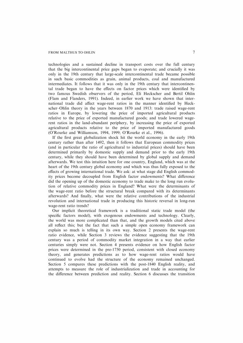
century rather than after 1492, then it follows that European commodity prices(and in particular the ratio of agricultural to industrial prices) should have beendetermined primarily by domestic supply and demand prior to the early 19thcentury, while they should have been determined by global supply and demandafterwards. We test this intuition here for one country, England, which was at theheart of the 19th century global economy and which was thus fully exposed to theeffects of growing international trade. We ask: at what stage did English commod-ity prices become decoupled from English factor endowments? What differencedid the opening up of the domestic economy to trade make to the long run evolu-tion of relative commodity prices in England? What were the determinants ofthe wage-rent ratio before the structural break compared with its determinantsafterwards? And finally, what were the relative contributions of the industrialrevolution and international trade in producing this historic reversal in long-runwage-rent ratio trends?Our implicit theoretical framework is a traditional static trade model (the

specific factors model), with exogenous endowments and technology. Clearly,the world was more complicated than that, and the growth models cited aboveall reflect this; but the fact that such a simple open economy framework canexplain so much is telling in its own way. Section 2 presents the wage-rentratio evidence, while Section 3 reviews the evidence suggesting that the 19thcentury was a period of commodity market integration in a way that earliercenturies simply were not. Section 4 presents evidence on how English factorprices were determined in the pre-1750 period, consistent with closed economytheory, and generates predictions as to how wage-rent ratios would havecontinued to evolve had the structure of the economy remained unchanged.Section 5 compares these predictions with the post-1840 English reality, andattempts to measure the role of industrialization and trade in accounting forthe difference between prediction and reality. Section 6 discusses the transition

FROM MALTHUS TO OHLIN 7

which the English economy underwent between 1750 and 1840, and Section 7concludes.

2. Wage-Rent Ratios in England Since 1500

Figure 1 plots our index of wage-land rent ratios in England from 1500 to 1936.The sources used are described in Appendix 1. Briefly, the nominal agriculturalwage series is based on recent work by Clark (2001, n.d.) for the 16th to the 18thcenturies, and on older sources for the 19th and 20th centuries (Fox, Bowley andWood, both in Mitchell, 1988). The land rent series uses Allen’s (1988) SouthMidlands data until 1831, and Thompson (1907) and Rhee (1949) thereafter. Theseries shows a large decline in wage-rent ratios between 1500 and about 1850, anda substantial rise thereafter. It is this reversal in distributional trends that we wishto explain.

3. Global Commodity Market Integration: The 19th Century Was Different

Since we want to offer an explanation for the rise in wage-rent ratios after 1800that discriminates between industrialization and trade as potential causes, weneed to be precise about exactly when Europe opened up to intercontinentaltrade in the sorts of goods that might have an effect on European factor prices.We are not primarily concerned with trade in goods like spices or silver, eventhough all trade should have some sort of an effect on factor prices in generalequilibrium; rather, we are concerned with trade in ‘competing commodities’ suchas grain or textiles, which might directly displace European production, and give

10

100

1000

1900

=10

0 (l

og s

cale

)

1500 1600 1700 1800 1900 2000 Year

1500-1936, 1900=100 (log scale)

Figure 1. English wage-rental ratio. Source: Appendix 1.


rise to the large-scale reshuffling of factors between sectors that might alterwages, profits or rents. This section stresses intercontinental trade, since it wasthe dramatically different factor endowments of the New World that wouldeventually place European land rents under sustained pressure, and contributeto the reversal in wage-rent ratios. Obviously within Europe there were regionsof relative land abundance and relative land scarcity, and the costs of tradebetween these regions had been declining for several centuries. For example,Jacks (2000) has documented substantial commodity market integration acrossthe North Sea and Baltic Sea between 1500 and 1800. But no amount of tradewith Prussia, for example, could have had the same impact on the Britisheconomy, or on British factor prices, as trade with the Americas eventually didin the 19th century.The costs of trading across frontiers will be reflected in price differentials for

homogenous goods in different markets, and a decline in these price differentialsprovides the clearest indication of international commodity market integration.Prior to the 19th century, there is no systematic evidence of inter-continental priceconvergence. For example, Figure 2 graphs the relationship between the averageprices received by the East India Company on its Asian textile sales in Europe,and the average prices it paid for those textiles in Asia. This textile trade wasextremely large and it was on the rise. Yet, there is no sign of declining mark-ups(where mark-ups include all trade costs, as well as any East India Companymonopoly profits) over the century between 1664 and 1769; trade expansion wasdue to outward shifts in demand and supply, rather than to commodity marketintegration (O’Rourke and Williamson, 2002a, b). This is not an isolated finding;indeed, somewhat surprisingly O’Rourke and Williamson (2002b) find no evidenceof intercontinental price convergence, over a much longer time period (1580–1800or so), even for very high-value-to-weight-ratio ‘non-competing’ commodities suchas cloves, pepper and coffee.

0

2

4

6

8

10

Sale

s pr

ice/

purc

hase

pri

ce

1660 1680 1700 1720 1740 1760

Year

1664-1759

Figure 2. Asian textile trade markups. Source: O’Rourke and Williamson (2002b).


The key trade driving down European rents in the late 19th century was thetrade in grain; unfortunately, we do not have intercontinental price gaps for grainsprior to 1800. However, Figure 3 plots Anglo-American wheat price gaps from1800 to 1999.1 The price gap fluctuated widely around an average of about 100percent between 1800 and 1840, but did not systematically decline. After 1840 itfell sharply, reaching negligible levels by the eve of World War I. The timing ofthis decline in price differentials coincides with the timing of the switch in policyfrom mercantilism to trade liberalism when Britain removed navigation acts,removed import prohibitions and lowered average tariffs from about 71 percent in1815, to about 54 percent in the 1830s, and to about 22 percent in the early 1840s,before moving to virtual free trade in 1846 (Williamson, 1990). This British pro-global lead was then followed in the 1860s on the European continent (Bairoch,1989). The timing of world commodity price convergence also coincides with thesustained decline in ocean freight rates documented by Harley (1988), and sup-ports his view that the new transport technologies of the 19th century were crucialin revolutionizing world trade, rather than the institutional factors stressed byNorth (1958), which had been in operation from an earlier date.2 Finally, it

0

50

100

150

200 Pe

rcen

t pri

ce g

ap, 3

yr

mov

ing

aver

age

0

10000

20000

30000

40000

50000

60000

70000

Impo

rts,

thou

sand

s of

cw

ts

1800 1820 1840 1860 1880 1900 1920 1940 1960 1980 2000Year

Anglo-American wheat price gap British imports of US wheat

Figure 3. Anglo-America wheat trade. Source: for price gaps, see footnote 1; for British wheat imports:Mitchell (1988).

1 The British data are Gazette averages through 1980, and are taken from Mitchell (1988). After 1980,

they are taken from the commodity price trends tables in the UK Annual Abstract of Statistics. The US

data for 1870–1913 are taken from O’Rourke (1997), where they are expressed in shillings per cwt; these

data are spliced on to the series in U.S. Department of Commerce (1975) for 1800–1870 and the US

Department of Agriculture series for 1914–1999 (http://usda.mannlib.cornell.edu/usda/usda.html).

2 Thus, the Industrial Revolution did not just have a direct impact on factor prices through its effects

on domestic technology; it also indirectly affected factor prices by promoting intercontinental trade.

Trade, in turn, influenced the Industrial Revolution, and we discuss these linkages in Section 6.


coincides with the emergence of large-scale wheat exports from the United States,as Figure 3 clearly shows.The evidence of Figure 3 could be replicated many times over: by the late

19th century it is difficult to find commodities and pairs of markets for whichthere is no evidence of powerful commodity market integration.3 To take justthree examples, London–Cincinnati percentage price differentials for bacon fellfrom 92.5 percent in 1870 to 17.9 percent in 1913; Liverpool–Bombay price differ-entials for cotton fell from 57 percent in 1873 to 20 percent in 1913; and London–Rangoon price differentials for rice fell from 93 to 26 percent over the same period(O’Rourke and Williamson, 1999, pp. 43–53). Commodity market integrationduring the century before World War I was a genuinely worldwide phenomenon,and it was immense.

4. What Determined English Commodity and Factor Prices Prior to 1750?

If sustained global commodity market integration only began in the 19th centurythen it follows that the distributional implications of international trade shouldonly have begun to manifest themselves some time between Waterloo and theGreat War. In order to test this hypothesis we gathered data on English factorendowments, commodity prices, productivity and factor prices from 1500 to 1936.For these four centuries, we were able to construct: the ratio of agricultural land tothe economy-wide labor supply (LANDLAB); the ratio of agricultural pricesto industrial prices (PAPM); the ratio of wage rates to farm land rents (WR); totalfactor productivity in agriculture (TFPAG); and labor productivity in manufactur-ing (INDPROD). The sources of these English data are described in Appendix 1.Figure 4 plots these five variables (expressed as natural logarithms) between

1500 and 1840, while Figure 5 shows their evolution between 1840 and 1936.The main argument of this paper emerges clearly from these figures. In bothperiods the land-labor ratio was trending down sharply. In a closed economy,this should have implied a falling wage-rental ratio. In principle, it should alsohave pushed up food demand relative to food supply, and raised the relativeprice of food. Figure 4 shows that both of these predictions held good for theearlier period. However, after 1840 the wage-rental ratio started to rise, despitean acceleration in the decline of land-labor ratios; while the relative price offood stopped rising, and eventually started to fall. Our argument is that after1840 commodity prices began to be exogenous to the British economy; andwage-rental ratios were no longer primarily driven by land-labor ratios, but

3 Continental European grain markets protected by defensive tariffs provide one exception in the late

19th century: see O’Rourke (1997). Defensive protection against an invasion of European

manufactures was even greater in Latin and North America, but it did not overturn the forces of

global integration caused by transport improvements (Blattman et al., 2002; Coatsworth and

Williamson, 2004; Williamson, 2002, 2005).


rather by trade (i.e., an exogenously determined relative price of food) and bythe Industrial Revolution (i.e., rising industrial productivity). But these are justassertions. Can econometric analysis bring further evidence to bear on theseissues?First, is it the case that English commodity prices were more closely linked to

English endowments prior to the 19th century? And if so, when did this traditional(closed economy) relationship break down? Figure 6 explores the question of whenthe structural break took place: it assumes a simple log-linear relationship betweenrelative commodity prices, PAPM, and the land-labor ratio LANDLAB, and plotsChow test statistics for every year between 1502 and 1935 to see where a structural

5.2

5.6

6.0

6.4

6.8

7.2

7.6

1500 1550 1600 1650 1700 1750 1800

LANDLAB

4.0

4.5

5.0

5.5

6.0

6.5

1500 1550 1600 1650 1700 1750 1800

WR

2.4

2.8

3.2

3.6

4.0

4.4

4.8

1500 1550 1600 1650 1700 1750 1800

PAPM

3.3

3.4

3.5

3.6

3.7

3.8

3.9

4.0

4.1

1500 1550 1600 1650 1700 1750 1800

INDPROD

3.6

3.7

3.8

3.9

4.0

4.1

4.2

4.3

4.4

1500 1550 1600 1650 1700 1750 1800

TFPAG

Figure 4. Raw data, 1500–1840. Source: Appendix 1.


break in this relationship is most likely to have taken place. There is a slow, hardlynoticeable rise in the test statistic between 1500 and 1700, followed by a significantrise from 1700 to 1750, and a larger rise from 1750 to 1800. This timing coincideswell with what we know about the gradual opening of the English economy to inter-national trade during the course of the 18th century: for example, the share ofexports in national income rose from 8.4 percent in 1700 to 14.6 percent in 1760 and15.7 percent in 1801 (Crafts, 1985, Table 6.6, p. 131). The figure suggests that tradi-tional links between relative commodity prices and endowments were already break-ing down during the 18th century, and we will have more to say about this inSection 6; however, the sharpest acceleration in the test statistic occurs between

4.0

4.2

4.4

4.6

4.8

5.0

5.2

5.4

5.6

1850 1875 1900 1925

LANDLAB

4.0

4.4

4.8

5.2

5.6

6.0

1850 1875 1900 1925

WR3

4.3

4.4

4.5

4.6

4.7

4.8

4.9

1850 1875 1900 1925

PAPM

3.8

4.0

4.2

4.4

4.6

4.8

5.0

5.2

1850 1875 1900 1925

INDPROD

4.3

4.4

4.5

4.6

4.7

4.8

4.9

1850 1875 1900 1925

TFPAG

Figure 5. Raw data, 1840–1936. Source: Appendix 1.


about 1800 and 1840. Figure 6 suggests that the best candidate for a structuralbreak is the second quarter of the 19th century, with the peak in the series occurringin 1838. Strikingly, this 1838 peak in Figure 6 is very similar to the timing of declinein both the Harley freight index and the UK–US grain price gap. Furthermore, it isconsistent with qualitative accounts regarding the liberalization of trade policywhich have long been a staple in the economic history literature. That is, the twodecades or so after 1815 were full of pro-globalization policy changes. Prior to 1828,grain imports were prohibited if domestic prices fell below a certain ‘port-closing’level, and during the early postwar years grain imports were effectively excludedmuch of the time. In 1828, the Duke of Wellington’s government replaced theseimport restrictions with tariffs which varied with the domestic price, a policy thatnot only lowered British grain prices but also increased the integration of Britishand Continental grain markets. Moreover, this adoption of the sliding scale tariffcame at the end of a decade which had seen several other moves towards freer trade:a reform of the Navigation Acts in 1822; tariff reductions across the board; and therepeal of more than 1100 tariff acts in 1825, the year in which the emigration ofskilled workers was once again authorized. Of course, prior to 1815 the French Warshad severely restricted international trade (Findlay and O’Rourke, 2002). In short,by 1838 there had already been a radical liberalization of British commercial policy(Williamson, 1990), and Britain stuck with that pro-globalization policy stance upto the more famous 1846 Repeal of the Corn Laws and beyond.4

0

200

400

600

800 F-

stat

istic

1500 1550 1600 1650 1700 1750 1800 1850 1900 1950 Year

Figure 6. Chow test statistics. Source: see text.

4 In a related paper, O’Rourke and Sollis (ongoing) search for the structural break using a variety of

more sophisticated methods, including recursive OLS, Markov switching and multiple break

models. They also conclude that there was a break in the relationship linking English relative

commodity prices, and English endowments, some time in the early 19th century.


Table 1 estimates a simple log-linear regression of PAPM on LANDLAB forthe initial, closed economy period, which we take to be 1500–1750. As expected,the coefficient is negative; moreover, the regression passes standard Engle–Grangercointegration tests at the 10 percent level.5 We are only interested in the long runrelationship between these two variables, and not in the short-run dynamicslinking them; the OLS result gives us a super-consistent estimate of this coefficient,given that the relationship is cointegrating.6 Figure 7 plots the natural logarithmof PAPM, and of its predicted value generated by this regression (labeledPAPMF). Thus, PAPMF represents the relative price of agricultural goods thatwould have prevailed had they continued to be determined by domesticendowments after 1750. Since land-labor ratios continued to decline in Britainafter 1750, the regression predicts that the relative price of food should have

Table 1. Explaining relative commodity prices, 1500–1750.

Dependent Variable: PAPM

Variable Coefficient Standard error

C 8.372 0.168

LANDLAB )0.764 0.024

R-squared 0.919 Sum of squared residuals 0.996

Adjusted R-squared 0.919 Log likelihood 337.837

S.E. of regression 0.063 Durbin–Watson stat 0.017

ADF (3 lags) )3.112 P(247)=0.0897; P(¥)=0.0860

Source: See text. Standard errors are Newey-West corrected.

2.5

3

3.5

4

4.5

5

5.5

Log

(PA

PM)

1500 1600 1700 1800 1900 2000Year

PAPMF PAPM

Figure 7. Actual and predicted PAPM. Source: see text.

5 Throughout, we calculate P-values for these cointegration tests using the program described in

MacKinnon (1996).

6 We also tried Johansen cointegration techniques, and these results are reported in a later footnote.


continued to rise, at an accelerating rate. But in fact it stopped rising somewherearound the middle of the 19th century, and then started to decline. Table 1 does avery good job of predicting the behavior of PAPM prior to the middle of the 18thcentury, but Figure 7 shows that it does a very poor job after the early or middleof the 19th century—consistent with the hypothesis that commodity prices becameuncoupled and delinked from domestic endowments by the mid-19th century, andwere determined on world markets thereafter.How were wage-rent ratios determined in pre-19th century England? In a closed

economy without trade, a decline in land-labor ratios should lead to a fall in thewage-rent ratio, and for standard Malthusian reasons. Rising industrial productiv-ity, due either to rising capital-labor ratios or to better industrial technology, shouldraise wage-rent ratios, for reasons stated earlier. The impact of better agriculturaltechnology on wage-rent ratios should depend on whether it was labor-saving orland-saving. Table 2 gives the results of regressing the wage-rent ratio (WR) onendowments (LANDLAB), on industrial productivity (INDPROD), and onagricultural productivity (TFPAG), for the years 1500–1750. (Once again, allvariables are expressed in natural logarithms.) As expected, the wage-rent ratio waspositively related to the land-labor ratio. As expected, it was also positively relatedto industrial productivity. The wage-rent ratio was negatively related to agriculturalproductivity, suggesting that technical change in early modern English agriculturetended to be labor-saving or land-using, which is what socialist critics of the enclo-sure movement have long maintained (Marx, 1867; Dobb, 1946), a position thathas found impressive support in recent empirical analysis (Allen, 1992: Chap. 11).7

7 The relationship is at the margins of cointegration, passing the Engle–Granger test at the 14 percent

level. We also used Johansen methods to search for cointegrating relationships between all five

variables (further details available on request). Both the trace and max-eigenvalue tests indicated

that there were 3 such relationships (at the 5 percent confidence interval). The data easily allowed

us to place a number of coefficient restrictions on the model (the P-value of the relevant LR test

being 0.67), and the results were as follows (standard errors in parentheses):

WR - 2.01 LANDLAB = 0;

(0.20)

PAPM + 0.75 LANDLAB = 0;

(0.03)

INDPROD - 0.70 LANDLAB - 1.88 TFPAG = 0

(0.13) (0.21)

The elasticity of PAPM with respect to LANDLAB is almost identical to that estimated by OLS

methods; while the elasticity of WR with respect to LANDLAB is somewhat bigger (2.01 as

opposed to 1.66). The interpretation of the third equation is straightforward: industrial productivity

depends not only on TFP in industry, but on capital-labor ratios there as well; it is therefore

sensitive to the intersectoral allocation of labor. Rising land-labor ratios or better agricultural

technology might well imply a higher demand for labor in agriculture, thus raising capital-labor

ratios in industry. It should be clear that the argument in the text would be qualitatively unaffected

if we used these estimates; in the absence of structural change, PAPM would have continued to rise

at the same rate as in Figure 7, and WR would have continued to fall (even more rapidly than in

Figure 8, since the Johansen elasticity of WR with respect to LANDLAB is higher), as the

land-labor ratio kept falling.


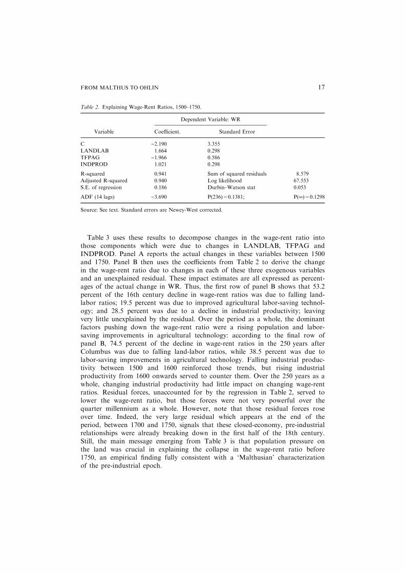
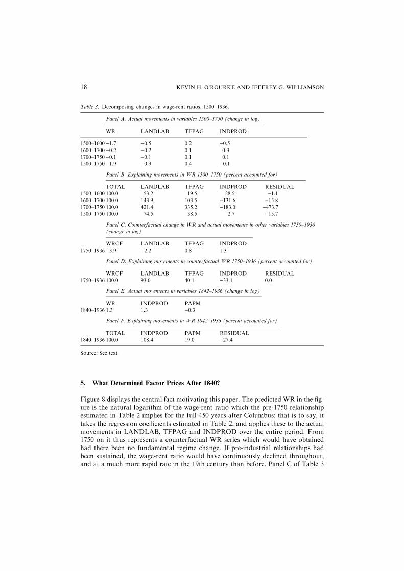
Table 3 uses these results to decompose changes in the wage-rent ratio intothose components which were due to changes in LANDLAB, TFPAG andINDPROD. Panel A reports the actual changes in these variables between 1500and 1750. Panel B then uses the coefficients from Table 2 to derive the changein the wage-rent ratio due to changes in each of these three exogenous variablesand an unexplained residual. These impact estimates are all expressed as percent-ages of the actual change in WR. Thus, the first row of panel B shows that 53.2percent of the 16th century decline in wage-rent ratios was due to falling land-labor ratios; 19.5 percent was due to improved agricultural labor-saving technol-ogy; and 28.5 percent was due to a decline in industrial productivity; leavingvery little unexplained by the residual. Over the period as a whole, the dominantfactors pushing down the wage-rent ratio were a rising population and labor-saving improvements in agricultural technology: according to the final row ofpanel B, 74.5 percent of the decline in wage-rent ratios in the 250 years afterColumbus was due to falling land-labor ratios, while 38.5 percent was due tolabor-saving improvements in agricultural technology. Falling industrial produc-tivity between 1500 and 1600 reinforced those trends, but rising industrialproductivity from 1600 onwards served to counter them. Over the 250 years as awhole, changing industrial productivity had little impact on changing wage-rentratios. Residual forces, unaccounted for by the regression in Table 2, served tolower the wage-rent ratio, but those forces were not very powerful over thequarter millennium as a whole. However, note that those residual forces roseover time. Indeed, the very large residual which appears at the end of theperiod, between 1700 and 1750, signals that these closed-economy, pre-industrialrelationships were already breaking down in the first half of the 18th century.Still, the main message emerging from Table 3 is that population pressure onthe land was crucial in explaining the collapse in the wage-rent ratio before1750, an empirical finding fully consistent with a ‘Malthusian’ characterizationof the pre-industrial epoch.

Table 2. Explaining Wage-Rent Ratios, 1500–1750.

Dependent Variable: WR

Variable Coefficient. Standard Error

C )2.190 3.355

LANDLAB 1.664 0.298

TFPAG )1.966 0.586

INDPROD 1.021 0.298




ADF (14 lags) )3.690 P(236)=0.1381; P(¥)=0.1298

Source: See text. Standard errors are Newey-West corrected.


5. What Determined Factor Prices After 1840?

Figure 8 displays the central fact motivating this paper. The predicted WR in the fig-ure is the natural logarithm of the wage-rent ratio which the pre-1750 relationshipestimated in Table 2 implies for the full 450 years after Columbus: that is to say, ittakes the regression coefficients estimated in Table 2, and applies these to the actualmovements in LANDLAB, TFPAG and INDPROD over the entire period. From1750 on it thus represents a counterfactual WR series which would have obtainedhad there been no fundamental regime change. If pre-industrial relationships hadbeen sustained, the wage-rent ratio would have continuously declined throughout,and at a much more rapid rate in the 19th century than before. Panel C of Table 3

Table 3. Decomposing changes in wage-rent ratios, 1500–1936.

Panel A. Actual movements in variables 1500–1750 (change in log)

WR LANDLAB TFPAG INDPROD

1500–1600 )1.7 )0.5 0.2 )0.51600–1700 )0.2 )0.2 0.1 0.3

1700–1750 )0.1 )0.1 0.1 0.1

1500–1750 )1.9 )0.9 0.4 )0.1

Panel B. Explaining movements in WR 1500–1750 (percent accounted for)

TOTAL LANDLAB TFPAG INDPROD RESIDUAL

1500–1600 100.0 53.2 19.5 28.5 )1.11600–1700 100.0 143.9 103.5 )131.6 )15.81700–1750 100.0 421.4 335.2 )183.0 )473.71500–1750 100.0 74.5 38.5 2.7 )15.7

Panel C. Counterfactual change in WR and actual movements in other variables 1750–1936

(change in log)

WRCF LANDLAB TFPAG INDPROD

1750–1936 )3.9 )2.2 0.8 1.3

Panel D. Explaining movements in counterfactual WR 1750–1936 (percent accounted for)

WRCF LANDLAB TFPAG INDPROD RESIDUAL

1750–1936 100.0 93.0 40.1 )33.1 0.0

Panel E. Actual movements in variables 1842–1936 (change in log)

WR INDPROD PAPM

1840–1936 1.3 1.3 )0.3

Panel F. Explaining movements in WR 1842–1936 (percent accounted for)

TOTAL INDPROD PAPM RESIDUAL

1840–1936 100.0 108.4 19.0 )27.4

Source: See text.


reports the change in this counterfactual wage-rent ratio series (WRCF) between1750 and 1936, as well as the actual changes in the exogenous variables which aredriving the counterfactual series. Panel D then decomposes the change in the count-erfactual series into the components explained by changes in each of the three exoge-nous variables. Declining land-labor ratios explain almost the entire decline in thecounterfactual series (93 percent); more rapid (labor-saving) technological progressin agriculture also helps push down counterfactual wage-rent ratios (40 percent), butthis agricultural productivity effect is almost entirely offset by the impact of evenmore rapid improvements in industrial productivity ()33 percent).If there had been no fundamental change in regime, 19th century wage-rent ratios

would have continued to decline rapidly, but this is not at all what happened. On thecontrary, Figure 8 shows that the wage-rent ratio actually declined at a far moresedate pace until 1850 or so, before turning around and increasing markedly. Whatexplains this dramatic departure from the historical norm? Was it the industrial rev-olution, which pulled workers into the cities at an accelerating pace, thus raisingwage-rent ratios? Or was it the growing internationalization of the British economy,effectively raising Britain’s land-labor ratio by importing land-intensive foodstuffsand manufacturing intermediates (e.g., cotton, wool and timber) produced on moreabundant land overseas? Or was it both?Table 4 estimates a (log-linear) open-economy model of the wage-rent ratio over

the period 1842–1936.8 This period was chosen since the previous two sectionssuggested that it was only after the late 1830s that the transition was complete

0

1

2

3

4

5

6

7lo

g

1500 1550 1600 1650 1700 1750 1800 1850 1900 1950

Year

Actual Predicted

Figure 8. Actual & predicted w/r. Source: see text.

8 O’Rourke and Williamson (2002c) show that while closed economy models similar to the one

estimated earlier work well before 1800, they do not work at all well from the 19th century on.

Similarly, open economy models work well for the later period, but not for the earlier one.


from a relatively closed economy to a relatively open one in which relativecommodity prices were effectively delinked from domestic endowments; 1842 wasalso the date of a major liberalization of the grain trade. In an open economy,WR could still be a function of INDPROD, TFPAG and LANDLAB (assumingthat the number of factors exceeds the number of traded goods), but it should alsobe a function of relative commodity prices PAPM, which are now taken asexogenous in a newly globalized world. The specific factors trade model predictsthat as the relative price of food declines, resources should be transferred out ofagriculture, and land rents (returns to the immobile factor) should fall relative towages (returns to the mobile factor): thus WR should be a negative function ofPAPM. TFPAG and LANDLAB are omitted from the regression since when equa-tions were estimated including them, the coefficients on TFPAG and LANDLABwere statistically insignificant, and the equations failed Engle–Granger cointegra-tion tests. We are thus left with a parsimonious specification in which the wage-rent ratio is a function of industrial productivity and relative commodity pricesalone. As Table 4 shows, WR was again positively related to industrial productiv-ity, and the estimated coefficient is almost exactly the same as that found inTable 2 for 1500–1750 (i.e., 1.04, as opposed to 1.02). Furthermore, WR was neg-atively related to the relative price of agricultural goods, just as trade theory sug-gests. The equation passes the Engle–Granger cointegration test at the 10 percentlevel. Again, we stress that we are only interested in the long-run relationshipslinking these variables, and OLS methods should provide us with good estimatesof these relationships given cointegration.9

Table 4. Explaining wage-rent ratios, 1842–1936.

Dependent Variable: WR

Variable Coefficient Standard Error

C 3.920 2.140

INDPROD 1.041 0.096

PAPM )0.868 0.406




ADF (1 lag) )3.562 P(89)=0.0914; P(¥)=0.0777

9 Again, we tried using Johansen methods to find cointegrating relationships between WR,

INDPROD and PAPM; the trace statistic indicated 1 relationship at the 5 percent confidence level.

Normalizing the coefficient on WR to unity, the estimate is as follows (standard errors in

parentheses):

WR + 3.63 PAPM - 0.70 INDPROD = 0

(0.79) (0.21)


Panel E of Table 3 reports the actual changes in WR, INDPROD and PAPMbetween 1842 and 1936, while Panel F decomposes the change in WR into thoseportions due to changing industrial productivity and changing relative prices.From the results in Panel F it might appear that the industrial revolution was thedominant actor in the story, while globalization was only a bit player. After all,the rise in industrial productivity accounted for all of the rise in the wage-rentratio after 1842, while falling relative agricultural prices accounted for ‘‘only’’ afifth of the rise (and the impact of PAPM was almost precisely offset by residualfactors). However, this decomposition is a grossly inaccurate reflection of theimpact on factor prices of Britain opening up to intercontinental trade betweenthe 1820s and 1840s, since the decomposition measures the impact of changingcommodity prices relative to an implicit counterfactual of no change in relativecommodity prices. In fact, the appropriate no-trade counterfactual is one of a con-tinued rise in relative agricultural prices (Figure 7), and it is against that counter-factual that the impact of the regime switch to openness should be gauged.Figure 9 supplies a far more accurate accounting of the relative impact of trade

and the industrial revolution in explaining the turn-about in wage-rent trends afterthe 1830s. It reports the actual behavior of the wage-rent ratio from 1842onwards (based on fitted values from the regression in Table 4) and the‘‘predicted’’ wage-rent ratio which would have applied had pre-1750 relationshipspersisted (based on fitted values from the regression in Table 2). While the wage-rent ratio in fact increased almost five-fold over the period, it would have declinedby more than 80 percent had it continued to evolve according to pre-1750

Footnote 9 Continued

The results are qualitatively, if not quantitatively, similar to those presented in Table 4. Using the

Johansen estimates would imply a much bigger elasticity of the wage-rental ratio with respect to

prices, and a smaller elasticity of the wage-rental ratio with respect to industrial productivity, than

those implied by Table 4. This would strengthen our argument (since we would then find that rising

industrial productivity had a smaller effect on the wage-rental ratio, and that commodity prices had

an even bigger effect).

Another partial test of the plausibility of these results comes from asking what simple trade theory

would predict about the size of the coefficients. Assume a two-sector specific factors model, with

food (A) produced by land and labor, and manufactured goods (M) produced by labor and capital.

We have: aRAd + aLAw = pA and aKMr + aLMw = pM where the aij’s are unit input requirements

of R (land), L (labor) and K (capital) into the two sectors, A and M; d, w and r are the returns to

land, labor and capital respectively; and pi is the price of good i. Totally differentiating both

equations, and making use of Jones (1971, p. 7, equation 1.11), it is easy to derive an algebraic

expression relating the percentage change in (w/d) to percentage changes in (pA/pM), (R/L) and (K/

L). As usual, the implied coefficients depend on cost shares in the two sectors, hij, and on

intersectoral labor allocation shares kLi. Assuming kLA = 0.25, kLM = 0.75, hKM = 0.4,

hRA = 0.5, and elasticities of substitution in agriculture (1.0) and industry (0.5), yields a predicted

coefficient on relative prices of )1.3, not so different from our OLS estimate ()0.87); and a

predicted coefficient of 1.04 on INDPROD (taken to be driven by K/L), which is identical to the

estimate we obtained in Table 4. In the Johansen framework, we are able to impose the restriction

that the coefficient on INDPROD is 1.04 (the relevant P-value is 0.17); in this case the elasticity of

WR with respect to PAPM becomes )2.71.


relationships. The figure also plots three counterfactual wage-rent ratio series. Thefirst, labeled ‘no industrial revolution,’ is again based on the estimated equation inTable 4, but holds the level of industrial productivity constant in every year (at its1842 level). Thus, it shows the wage-rent ratios which would have obtained hadrelative commodity prices evolved in the way they did, but had there been noimprovement in industrial productivity from 1842 onwards. As can be seen, ifthere had been no increase in industrial productivity over that century, the wage-rent ratio would have remained roughly constant throughout—rising up to 1936by a mere 27 percent, rather than recording an actual increase of 394 percent. Pre-sumably, this is the channel of causation—from the industrial revolution to risingwage-rent ratios—which would have been favored by Jones, Galor and Weil,Lucas and other theorists, had they addressed this relative factor price issueexplicitly.10

The second series, labeled ‘no trade,’ also uses the coefficients which were esti-mated in Table 4. It assumes that the English economy remained relatively closedto international trade, and, to be more precise, that relative commodity prices con-tinued to be determined by domestic factor endowments after the 1830s. Thiscounterfactual thus allows INDPROD to evolve as it did, but substitutes thecounterfactual PAPMF series in Figure 7 for the actual PAPM series. As can beseen from Figure 9, if there had been no open economy forces causing relativecommodity prices to diverge from their historical trajectory the wage-rent ratiowould have remained relatively constant between 1842 and 1936, increasing by amere 80 percent, rather than by 394 percent as actually occurred. Figure 9 sug-gests that globalization and the industrial revolution had roughly equal effects onwage-rent ratios throughout this period: the two counterfactual series are

0

100

200

300

400

500

1840

=10

0

1840 1860 1880 1900 1920 1940 Year

No industrial revolution

No trade

No industrial revolution or trade

Actual (fitted values)

Predicted (pre-1750 model)

1842-1936

Figure 9. Actual & counterfactual w/r. Source: see table.

10 In fact, several papers in this literature (e.g. Galor and Weil, 2000; Jones, 2001; Galor and

Mountford, 2002) assume that returns to land are zero for reasons of analytical tractability.


remarkably close to each other. Finally, the ‘no industrial revolution and no trade’series holds INDPROD constant as before, and also substitutes PAPMF forPAPM as in the ‘no trade’ counterfactual. In this final counterfactual, the wage-rent ratio actually falls by 54 percent between 1840 and 1936, and at almost thesame rate as if pre-1750 relationships had been maintained.These counterfactuals invite two conclusions. First, industrial revolutionary

forces and the opening up of the English economy to trade together explain thehistoric reversal in long-run wage-rent ratio trends from Columbus to World WarII. If industrial productivity had failed to increase, and if relative commodityprices had continued to evolve as they had done prior to 1750, then the wage-rentratio would have continued to decline after the 1830s as it had since 1500, and bya substantial amount. However, once INDPROD and PAPM are allowed toevolve as they actually did, our econometric model replicates the actual rise inwage-rent ratios which took place after 1840. Second, and just as important, whilethe long-run turnaround in wage-rent ratio trends can be explained partly byindustrial revolutionary forces, it is also explained by the open economy forcesidentified long ago by Eli Heckscher and Bertil Ohlin. Comparing the ‘no trade’and ‘no industrial revolution’ series in Figure 9, it would appear that trade wasjust as important as industrial revolutionary forces in explaining the historic rela-tive factor price turn-around. A closed economy account of the revolutionarychange in growth and distribution performance during the 19th century misseshalf the story.

6. The Transition, 1750–1840

We have argued that Britain underwent two important regime switches during thelate 18th and early 19th centuries, not just one. The first was a transition to mod-ern industrial growth and the second was a transition towards a more open trad-ing environment. These regime switches were not abrupt, but rather took placeover a number of decades. Also, the two transitions were almost certainly con-nected. This section will elaborate on these two issues.Traditional economic history has always taught that the Industrial Revolution

marked a sharp and ‘‘revolutionary’’ discontinuity. The older evidence seemed tosupport this view; for example, Hoffmann’s (1955) data show a dramatic acceler-ation of industrial output after 1770. More recent work, however, has foundthat aggregate growth and technical change were much slower between 1770 and1830 than had been previously thought (e.g., Crafts and Harley, 1992), withtechnical change largely concentrated in a number of key industries. Moreover,the aggregate growth rate had been steadily increasing since the beginning of the18th century. Thus, ‘‘the origins of modern economic growth extended over alonger time period and a wider geographical area than are traditionally encom-passed in studies of the Industrial Revolution’’ (Harley and Crafts, 2000, pp.820–821). Furthermore, there is another tradition that focuses on pre-factorycottage industry development, so-called proto-industrialization. This recent


scholarship has encouraged some to discard the phrase ‘‘industrial revolution’’entirely!While the price gap evidence outlined in Section 3 certainly documents a stark

contrast—no intercontinental price convergence before 1800, but substantial priceconvergence thereafter—it is important to note that the move to a more open Brit-ish economy had also been taking place over a long period. To repeat, the shareof exports in British national output gradually rose from 8.4 percent in 1700 to14.6 percent in 1760, 15.7 percent in 1801, and 19.6 percent in 1851 (Crafts, 1985,Table 6.6, p. 131). Furthermore, the role of intercontinental trade was alsoincreasing throughout the 18th and early 19th centuries: Europe took 85.3 percentof English exports in 1700–1701, but only 77 percent in 1750–1751, 49.2 percent in1772–1773, and 30.1 percent in 1797–1798. The Americas (the source of abundantland) were the most important overseas destination, with their share of totalexports rising from 10.3 to 57.4 percent over the same period (O’Brien and Enger-man, 1991, Table 4, p. 186). Figure 6 indicated that traditional ‘‘Malthusian’’ rela-tionships between English prices and endowments were already breaking downduring the 18th century, consistent with this gradual opening of the economy.True, wars continuously served to interrupt the contribution of long run funda-mentals pushing international commodity market integration. For example,O’Rourke and Williamson (2002b) find a spike in the Euro–Asian clove price gapwhich coincided with the Seven Years War (1756–1763), and an increase in coffeeand black pepper price gaps during the 1790s which coincided with the outbreakof the French and Napoleonic Wars. The Pax Britannica that prevailed afterWaterloo allowed those fundamentals to exert their full impact. These includedthe technological breakthroughs in transport which were crucial in driving downfreight rates so dramatically in the 19th century (Harley, 1988).Finally, the two revolutions which we argue were responsible for reversing the

long run decline in wage-rent ratios were connected in a number ofways—although the precise nature of these links remains a subject of livelydebate.11 Most obviously, and as noted earlier, the innovations which drove downfreight rates—notably the metal steamship—depended on the steam engine anddevelopments in metallurgy which together constituted some of the most notabletechnological breakthroughs of the Industrial Revolution. But the causation mayalso have gone the other way around, from trade to the Industrial Revolution.While it is clear that the industrial revolution was supply-driven, and that exportdemand was therefore not the cause of it in any old-fashioned Keynesian sense(Mokyr, 1977), and while Marxist accounts of the industrial revolution, which link

11 For a recent survey of the historiography, see Morgan (2000). One theorist has actually constructed

a computable model of the process and used it to decompose the sources of the British industrial

revolution into trade and technology forces (Stokey, 2001). Testing such a model against

competitors is, of course, a difficult task. In any case, economists have had an equally difficult (and

contentious) time trying to disentangle the late 20th century impact of globalization on growth and

inequality.


British accumulation to profits derived from the colonial trade, do not withstandempirical scrutiny either (O’Brien, 1982), it is difficult to imagine that Englishindustrial growth between 1750 and 1850 would have been as rapid as it was with-out ample and elastic supplies of imported raw materials such as cotton, and theability to sell industrial output in overseas markets (Findlay, 1982, 1990; O’Brienand Engerman, 1991). Overseas markets were in fact far more important forindustry than for the economy as a whole: the export share in gross industrialoutput was 24.4 percent in 1700 (the economy-wide share was 8.4 percent), and34.4 percent in 1801 (the economy-wide share was 15.7 percent; O’Brien andEngerman, 1991, p. 188). Between 1780 and 1801, the increase in industrialexports was 46.2 percent of the increase in gross industrial output; in 1801,exports were 24 percent of iron output, and an astonishing 62 percent of cottonoutput. While no scholar has quantified what would have happened to Britishinvestment incentives had industrialists been forced to sell their output solely ondomestic markets, and source all their raw materials domestically, the direction ofthe effect seems obvious. Without trade, the prices of manufactures would havedeclined by more than they actually did, and manufacturing inputs would havebeen far more expensive. Thus, profitability and (presumably) investment wouldhave been lower.12 Furthermore, an elastic supply of raw cotton to the Britisheconomy required not only elastic supplies of New World land, but elastic suppliesof slave labor as well. Thus, the British Industrial Revolution was intimatelybound up with the Triangular Trade linking Africa, Europe and the Americas(Findlay, 1990).

7. Conclusion

This paper has provided evidence of a dramatic structural break in European longrun relative factor price trends which coincided with the more familiar breakwhich occurred in living standards and aggregate productivity behavior. If thewage-rent ratio had continued to follow the same laws of motion after 1750 asbefore it would have declined continuously throughout the 19th and early 20thcenturies, and at an accelerating rate as population growth increased and theland-labor ratio fell ever more dramatically. Instead, the decline stopped and thetrends reversed, with a modern rise starting sometime after 1850.We have argued that this reversal in wage-rent ratio trends was due not only

to the industrial revolution, but to the opening of the English economy to trade.Evidence on falling transport costs, rising liberal policy, evaporating interna-tional commodity price gaps, rising trade shares, and the relationship betweencommodity prices and factor endowments all suggest that the English economybecame much more open to trade during the 18th and early 19th centuries, and

12 In addition, textile fibers such as wool were less easily mechanized than raw cotton, making a

counterfactual switch from imported cotton to domestic wool very difficult.


particularly during the quarter century or so after Waterloo. By the middle ofthe 19th century relative commodity prices no longer evolved as if they weredetermined by English factor endowments; relative agricultural prices stoppedtheir secular rise, and eventually even started to decline. We have shown thattrade was just as important as rising industrial productivity in explaining thereversal in wage-rent ratio trends after 1840. Factor price ratios would not haveincreased dramatically in the absence of industrial revolutionary forces; norwould they have increased dramatically had relative commodity prices continuedto be determined by domestic factor endowments, as they had been for the cen-turies before 1750.While this is a paper about England, there is some suggestive American evidence

which reinforces our conclusions. In a closed economy environment, the easternAmerican seaboard should have seen their wage-rental ratios fall as their popula-tions grew and land-labor ratios fell; in an open economy environment, trade shouldhave pushed up still farther the relative price of food and other resource-intensiveproducts in which the region had a comparative advantage, and thus reinforced theimpact of population growth, leading to even more rapid declines in the wage-rentalratio. Thus, in the closed economy period wage-rental ratios in Britain and the USshould have moved in the same direction (downward), while in the open economyperiod they should have diverged. The data on pre-1800 US wage-rent ratios aresparse, but what we have is consistent with these speculations. Thus, as Figure 10shows, in Connecticut free wage-rent ratios more than halved between the 1680s andthe late 1750s, and fell again in the decades before the Revolution (Williamson andLindert,1980, p. 21); while in South Carolina the trend in the ratio of slave prices toland values was broadly downwards during the last three quarters of the 18th

50

100

150

200

250

300

1757

=10

0

1685 1695 1705 1715 1725 1735 1745 1755 1765 1775 1785 1795

Year

ConnecticutSouth Carolina

1757=100

Figure 10. Wage-rental ratios 1685–1798. Souce: see text.


century (Mancall et al., 2001, 2002), at least if one ignores the spike in the years justbefore the Revolution. Unlike in England, this trend did not reverse after the emer-gence of large-scale intercontinental trade in basic commodities; rather, the USwage-rental ratio fell by almost 60 percent between 1870 and the Great War (O’Rou-rke et al., 1996; O’Rourke and Williamson, 1999).While this paper offers strong evidence that trade produced distributional

regime shifts during this period, we think its importance is understated. Afterall, we have ignored the possibility that the industrial revolution may itselfhave been intimately connected with the development of international tradeduring the 18th and early 19th centuries. Without the possibility of interconti-nental trade, industrial productivity would almost certainly have increased byless than it actually did during the industrial revolution: trade may not havekick-started the First Industrial Revolution, but it surely played an indispens-able supporting role.13 Open economy forces must have played an even moreimportant role after 1750 than our already-impressive econometric resultssuggest.

Acknowledgments

We have been helped with the wage-rent data by Greg Clark as well as by theexcellent research assistance of Darya Zhuck. In addition, the comments ofStephen Broadberry and Louis Cullen are gratefully acknowledged, as are thoseof participants at the Ohlin Conference (Stockholm, October 14–16, 1999), theSound Conference (Copenhagen, March 1, 2002), ERWIT 2002 (Munich, June14–17, 2002), the ISSC/HII Conference on ‘‘Past and Present: Long-term Per-spectives on the World Today’’ (Dublin, October 18, 2002), the NBER ITIWinter Institute (Palo Alto, December 7, 2002), the Minerva Center Conferenceon ‘‘From Stagnation to Growth’’(Rorschach, Switzerland, May 2–4, 2003);and seminar participants at ANU, Glasgow, Gotenborg, Harvard, Humboldt,Illinois, London School of Economics, Melbourne, New South Wales, Stock-holm School of Economics, Western Australia, and the Economic and SocialResearch Institute, all of whom heard early and preliminary versions of thispaper. O’Rourke is an IRCHSS Government of Ireland Senior Fellow andacknowledges the generous funding of the Irish Research Council for theHumanities and Social Sciences. Williamson acknowledges financial supportfrom the National Science Foundation SES-0001362. The usual disclaimerapplies.

13 Indeed, Acemoglu et al. (2002) have offered new evidence recently that participation in the Atlantic

economy was essential in making modern Western European growth possible before 1850.


Appendix 1. English Wages, Land Rents, Inter-Sectoral Terms of Trade,

Land-Labor Ratios and Sectoral Productivity 1500–1936

Nominal Agricultural Wages 1500–1936 (1900@ 100)

1500–1670: Male day wages in agriculture, pence per day; reported decadal, inter-polated geometrically to get annual; from Clark, G. The Long March of History:Farm Laborers’ Wages in England 1208–1850, Mimeo, Davis (n.d.): University ofCalifornia, Table 4, p. 26.1670–1851: ‘‘Winter’’ farm wages, pence per day; annual; from Clark, G. (August2001). ‘‘Farm Wages and Living Standards in the Industrial Revolution: England,1670–1850,’’ Economic History Review 54(3), pp. 477–505.1851–1902: Average weekly cash wages of ordinary laborers paid 67 farms in Eng-land and Wales, shillings per week; annual; from Wilson Fox, A. (1903). ‘‘Agricul-tural Wages in England and Wales During the Last Fifty Years,’’ Journal of theRoyal Statistical Society 66(2) pp. 273–359 and Appendix II, pp. 331–332.1902–1914: Bowley and Wood’s index of average agricultural wages, England andWales, in a normal week; annual index (1891 ¼ 100); taken from Mitchell, B. R.(1988). British Historical Statistics. Cambridge: Cambridge University Press, pp.158–159; original source: Bowley, A. L. (1937). Wages and Income Since 1860.Cambridge.1914–1920: Weekly wage rate in agriculture, England and Wales, in July; annualindex (July 1914 ¼ 100); taken from Mitchell (1988), p. 160; original source:Bowley, A. L. (1921). Prices and Wages in the United Kingdom, 1914–1920.Oxford: Oxford University Press.1920–1936: Weekly wage rate in agriculture, England and Wales; annual index(1924 ¼ 100); taken from Mitchell (1988), p. 160; original source: Ramsbottom, E. C.(1935). ‘‘The Course of Wage Rates in the United Kingdom, 1921–34,’’ Journal ofthe Royal Statistical Society XCVIII and similar article for 1934–1937 in ibid.

Nominal Farm Land Rents 1500–1936 (1900@ 100)

Index A

1500–1831: Land rental values, England average, £/acre; from Clark, G. (Decem-ber 2002). ‘‘Land Rental Values and the Agrarian Economy: England and Wales,1500–1912,’’ European Review of Economic History 6(3), pp. 281–308, Table 8; val-ues are given for 1500–39 (taken to be 1520), 1540–59 (1550), 1560–79 (1570) and1580–99 (1590); reported by decade for the 17th century; reported at 5 yearlyintervals from 1700 onwards; interpolated geometrically to get annual; rents areassumed constant from 1500–1520, in line with the data on land and farmhouserental values in Clark, G. (October 2001). ‘‘The Secret History of the IndustrialRevolution,’’ Mimeo, Table 2, p. 15; and also in line with the data in Allen, R. C.(February 1988). ‘‘The Price of Freehold Land and the Interest Rate in the


Seventeenth and Eighteenth Centuries,’’ Economic History Review XLI (1), pp. 33–50, discussed below under Index C.1831–1870: Annual; from Thompson, J. (December 1907). ‘‘An Inquiry into theRent of Agricultural Land in England and Wales during the Nineteenth Century,’’Journal of the Royal Statistical Society, LXX, Appendix, Table A, p. 612.1871–1900: Annual; an unweighted average of Thompson (1907) and Rhee, H. A.(1949). The Rent of Agricultural Land in England and Wales. London: CentralLandowners Association, Appendix Table 2, pp. 44–45.1900–1936: Annual; Rhee (1949).

Index B

Alternative index 1690–1914: Annual; linked forwards and backwards to the restof Index A above: Turner, M. E., J. V. Beckett, and B. Afton, (1997). AgriculturalRent in England 1690—1914. Cambridge: Cambridge University Press, AppendixTable A2.2, pp. 314–318.

Index C

Alternative index 1500–1831: South Midlands average rent, shillings per acre; byquarter century, interpolated geometrically; taken from Allen (1988), Table 2, p.43.1831–1936: As Index A above; annual.

Inter-Sectoral Terms of Trade, Pa/Pm (1900@ 100): Pa 1316–1938

1316–1450: Exeter wheat; annual; from Mitchell B. R., and P. Deane, (1962).Abstract of British Historical Statistics. Cambridge: Cambridge University Press,pp. 484–486.1450–1640: ‘‘Average—all agricultural products,’’ including grains, other arablecrops, livestock and animal products; reported decadal, interpolated geometricallyto get annual; from J. Thirsk (ed.) (1967). The Agrarian History of England andWales, Volume IV: 1500–1640. Cambridge: Cambridge University Press, TableXIII, p. 862.1640–1749: ‘‘Average—all agricultural products,’’ including grains, other fieldcrops, livestock and animal products; reported decadal, interpolated geometricallyto get annual; from J. Thirsk (ed.) (1985). The Agrarian History of England andWales, Volume V: 1640–1750. Cambridge: Cambridge University Press, Table XII,p. 856.1749–1805: Wheat; reported decadal, interpolated geometrically to get annual;from Deane P. and W. A. Cole (1962). British Economic Growth 1688–1959, 2ndedn. Cambridge: Cambridge University Press, Table 23, p. 91.


1805–1913: Total agricultural products; annual; from Mitchell and Deane (1962),pp. 471–473.1913–1938: Total food; annual; from Mitchell and Deane (1962), p. 475.

Inter-Sectoral Terms of Trade, Pa/Pm (1900@ 100): Pm 1450–1938

1450–1640: ‘‘Industrial products’’; reported decadal, interpolated geometrically toget annual; from Thirsk (1967), Table XIII, p. 862.1640–1749: ‘‘Industrial products’’; reported decadal, interpolated geometrically toget annual; from Thirsk (1985), Table XII, p. 856.1749–1796: ‘‘Other prices’’ (equals unweighted average of Schumpeter’s producergoods); annual; from Deane and Cole (1962), Table 23, p. 91.1796–1938: Price indices of merchandise exports (equals Imlah and Board ofTrade, linked on 1913); from Mitchell and Deane (1962), pp. 331–332.

Land/Labor Ratios (1900@ 100): Total Economy-Wide Labor Force 1500–1940

Post-1840

1841–1951: ‘‘Total occupied,’’ males and females; reported for census dates, inter-polated geometrically to get annual (including the missing years 1932–1936); fromMitchell and Deane (1962), pp. 60–61.

Pre-1841

Labor force or population age distribution estimates do not exist for the periodprior to the late 18th century. Thus, we simply link the population totals up to1841 with the economy-wide labor force totals 1841–1936 (e.g., we assume the 1841labor participation rate was constant between 1560 and 1840, and at the 1841 rate).Population 1541–1841: England; annual; from Wrigley, E. A. and R. S. Schofield.(1981). The Population History of England, 1541–1871. Cambridge: CambridgeUniversity Press, Table A3.3, pp. 531–534.Population 1500–1541: Assumes that growth was at the rate suggested by Wrigleyand Schofield (1981), p. 737.

Land/Labor Ratios (1900@ 100): Land in Agriculture 1500–1940

Post-1866

1867–1936: Acreage in crops; Great Britain; annual: from Mitchell and Deane(1962), pp. 78–79.


Pre-1867

In his seminal piece on population in pre-industrial England, Ronald D. Lee(‘‘Population in Preindustrial England: An Econometric Analysis,’’ QuarterlyJournal of Economics 87(4), pp. 581–607) quotes Postan to justify his assumptionof a constant farm land endowment: ‘‘By 1066 the occupation of England by theEnglish had gone far enough to have brought into cultivation . . . most of the areaknown to have been occupied in later centuries of English history.’’ (Postan, M. M.(1966). ‘‘Medieval Agrarian Society in Its Prime’’ in H. J. Habakkuk andM. M. Postan (eds.), Cambridge Economic History of Europe, Vol. I, 2nd edn.,Chapter VII, Part 7. Cambridge: Cambridge University Press, pp. 567–568. Wemake the same assumption.

Manufacturing Productivity (1900@ 100)

1869–1936: Manufacturing output divided by manufacturing employment; annual(with interpolations between 1913 and 1920); taken from Broadberry, S. N.(1997). The Productivity Race: British Manufacturing in International Perspective,1850–1990 Cambridge: Cambridge University Press, Appendix 3, pp. 42–44.1700–1869: Industrial production divided by industrial labor force. Industrial pro-duction taken from Crafts, N. F. R. and C. K. Harley. (November 1992). ‘‘OutputGrowth and the British Industrial Revolution: A Restatement of the Crafts-HarleyView,’’ Economic History Review XLV(4), pp. 703–730, ‘revised best guess’,Table A3.1, pp. 725-727; annual. Industrial labor force based on applying esti-mates of the industrial share of the labor force to the annual labor force esti-mates above. Crafts, N. F. R. (1985). British Economic Growth During theIndustrial Revolution. Oxford: Clarendon Press, Table 3.6, pp. 62–63, gives esti-mates of the industrial share of the male labor force for 1700, 1760, 1800, 1840and 1870. Data for intervening years are generated by geometric interpolation.The procedure assumes that the industrial share of the female labor force wassimilar to that of the male labor force.1500–1700: Non-agricultural output divided by non-agricultural labor force. Basedon data given in Clark (October 2001). Data on nominal GDP are taken from hisTable 3, pp. 19–20, and are deflated using the GDP deflator in his Table 7, pp.30–31. Real GDP is then divided into its agricultural and non-agricultural compo-nents by assuming that these are proportional to the wage bills in the two sectors(which is equivalent to assuming that the ratio of the average products in the twosectors is equal to the ratio of the marginal products in the two sectors). The ratioof the wage bill in the two sectors is derived using the data on sectoral wages andthe farm share of the labor force, given in Table 1, pp. 8–9 (and, following Clark,p. 7, letting the non-farm wage be the average of urban craftsman and laborerwages). The resulting output series is divided by the non-agricultural labor force,derived using Clark’s farm share of the labor force and the annual labor forceseries described above.


References

Acemoglu, D., S. Johnson, and J. Robinson. (2002). ‘‘The Rise of Europe: Atlantic Trade, Institutional

Change and Economic Growth,’’ CEPR Discussion Paper 3712, London: CEPR.Allen, R. C. (1988). ‘‘The Price of Freehold Land and the Interest Rate in the Seventeenth and Eigh-

teenth Centuries,’’ Economic History Review 41 (February), 33–50.Allen, R. C. (1992). Enclosure and the Yeoman. Oxford: Clarendon Press.Bairoch, P. (1989). ‘‘European Trade Policy, 1815–1914,’’ in Mathias P., and Pollard S. (eds.), The

Cambridge Economic History of Europe. Vol. III. Cambridge: Cambridge University Press.Blattman, C., M. A. Clemens, and J. G. Williamson. (2002). ‘‘Who Protected and Why? Tariffs the

World Around 1870–1937,’’ paper presented to the Conference on the Political Economy of Global-

ization. Trinity College, Dublin (August 29–31).Clark, G. (n.d.). ‘‘The Long March of History: Farm Laborers’ Wages in England 1208–1850,’’ mimeo,

Davis: University of California.Clark, G. (2001). ‘‘Farm Wages and Living Standards in the Industrial Revolution: England, 1670–

1850,’’ Economic History Review 54 (August), 477–505.Coatsworth, J. H., and J. G. Williamson. (2004). ‘‘The Roots of Latin American Protectionism:

Looking Before the Great Depression,’’ in Estevadeordal, A., D. Rodrik, A. Taylor, and A. Velasco

(eds.), FTAA and Beyond: Prospects for Integration in the Americas. Cambridge, MA: Harvard

University Press.Crafts, N. F. R. (1985). British Economic Growth During the Industrial Revolution. Oxford: Clarendon Press.Crafts, N. F. R. (1994). ‘‘The Industrial Revolution,’’ in R. Floud and D. McCloskey (eds.), The

Economic History of Britain Since 1700, Vol. 1. Cambridge: Cambridge University Press.Crafts, N. F. R., and C. K. Harley. (1992). ‘‘Output Growth and the Industrial Revolution: A Restate-

ment of the Crafts–Harley View,’’ Economic History Review 45(4), 703–730.Dobb, M. (1946). Studies in the Development of Capitalism. London: Routledge and Kegan Paul.Flam, H., and M. J. Flanders (1991). Heckscher-Ohlin Trade Theory. Cambridge, MA: MIT Press.Findlay, R. (1982). ‘‘Trade and Growth in the Industrial Revolution,’’ in Kindleberger, C. P., and

G. Di Tella (eds.), Economics in the Long View: Essays in Honor of W.W. Rostow New York: New

York University Press.Findlay, R. (1990). ‘‘The ‘Triangular Trade’ and the Atlantic Economy of the Eighteenth Century: A

Simple General-Equilibrium Model,’’ Essays in International Finance 177, International Finance

Section, Department of Economics, Princeton University.Findlay R., and K. H. O’Rourke. (2002). ‘‘Commodity Market Integration 1500–2000,’’ in Bordo, M.,

A. M. Taylor, and J. G. Williamson (eds.), Globalization in Historical Perspective Chicago:

University of Chicago Press.Galor, O., and A. Mountford. (2002). ‘‘Why are a Third of People Indian and Chinese? Trade, Indus-

trialization and Demographic Transition,’’ CEPR Discussion Paper 3136, London: CEPR.

Total Factor Productivity in Agriculture

1500–1911: Clark (forthcoming 2002), Table 9, p. 48; data for 1520, 1550, 1570,1590; decadal from 1605; interpolated to get annual. We assume that the 1520–1550growth rate applied to 1500–1520.1911–1936: Derived assuming constant growth rate of 0.4% p. a. 1911–1924; 2.1%p. a. 1924–1936. Based on Matthews, R. C. O., C. H. Feinstein, and J. C. Odling-Smee.(1982). British Economic Growth 1856–1973 (Stanford, CA: Stanford UniversityPress), Table L.2, p. 607 and Table I.3, p. 598. The calculation assumes that the1899–1913 growth rate persisted until 1924.


Galor, O., and D. N. Weil. (2000). ‘‘Population, Technology, and Growth: From Malthusian Stagna-

tion to the Demographic Transition and Beyond,’’ American Economic Review 90 (September): 806–

828.Goodfriend M., and J. McDermott. (1995). ‘‘Early Development,’’ American Economic Review 85

(March), 116–133.Hansen, G. D., and E. C. Prescott. (2002). ‘‘Malthus to Solow,’’ American Economic Review 92

(September), 1205–1217.Harley, C. K., (1988). ‘‘Ocean Freight Rates and Productivity, 1740–1913: The Primacy of Mechanical

Invention Reaffirmed,’’ Journal of Economic History 48 (December), 851–876.Harley, C. K., and N. F. R. Crafts. (2000). ‘‘Simulating the Two Views of the British Industrial Revo-

lution,’’ Journal of Economic History 60 (September), 819–841.Hoffmann, W. G. (1955). British Industry, 1700–1950. Oxford: Basil Blackwell.Jacks, D. (2000). ‘‘Market integration in the North and Baltic Seas, 1500–1800,’’ LSE Working Papers

in Economic History 55/00, London School of Economics, London (April).Jones, C. I. (2001). ‘‘Was the Industrial Revolution Inevitable? Economic Growth Over the Very Long

Run,’’ Advances in Macroeconomics 1(2), article 1.Jones, R. W. (1971). ‘‘A Three-Factor Model in Theory, Trade, and History,’’ in Bhagwati, J. et al.

(eds.), Trade, Balance of Payments, and Growth. Amsterdam: North-Holland.Lucas, R. (1999). The Industrial Revolution: Past and Future, mimeo. University of Chicago, Depart-

ment of Economics.MacKinnon, J. G. (1996). ‘‘Numerical Distribution Functions for Unit Root and Cointegration Tests,’’

Journal of Applied Econometrics 11(6) November–December: 601–618.Malthus, T. R., (1826). An Essay on the Principle of Population. Cambridge: Cambridge University

Press.Mancall, P. C., J. L. Rosenbloom, and T. Weiss. (2001). ‘‘Slave Prices and the South Carolina Econ-

omy, 1722–1809,’’ Journal of Economic History 61 (September), 616–639.Mancall, P. C., J. L. Rosenbloom, and T. Weiss. (2002). ‘‘Agricultural Labor Productivity in the Lower

South, 1720–1800’’, Explorations in Economic History 39 (October): 390–424.Marx, K. (1867). Capital, trans. S. Moore and E. Aveling, 3 Vols., 1867–1894, Vol. i. New York: Ran-

dom House, 1906.Mitchell, B. R. (1988). British Historical Statistics. Cambridge: Cambridge University Press.Mokyr, J. (1977). ‘‘Demand vs. Supply in the Industrial Revolution,’’ Journal of Economic History 37,

981–1008.Mokyr, J. (1990). The Lever of Riches: Technological Creativity and Economic Progress. New York:

Oxford University Press.Morgan, K. (2000). Slavery, Atlantic Trade and the British Economy 1660–1800. Cambridge: Cambridge

University Press.North, D. C. (1958). ‘‘Ocean Freight Rates and Economic Development 1750–1913,’’ Journal of

Economic History 18 (December): 538–555.O’Brien, P. K. (1982). ‘‘European Economic Development: The Contribution of the Periphery,’’

Economic History Review 35 (February), 1–18.O’Brien, P. K., and S. L. Engerman. (1991). ‘‘Exports and the Growth of the British Economy from

the Glorious Revolution to the Peace of Amiens,’’ in Solow B. L. (ed.), Slavery and the Rise of the

Atlantic System. Cambridge: Cambridge University Press, pp. 177–209.O’Rourke, K. H. (1997). ‘‘The European Grain Invasion, 1870–1913,’’ Journal of Economic History 57

(December), 775–801.O’Rourke K. H., and R. Sollis. (ongoing). ‘‘Globalisation, endowments and factor prices in England

1500–1936,’’ mimeo.O’Rourke, K. H., A. M. Taylor, and J. G. Williamson. (1996). ‘‘Factor Price Convergence in the Late

Nineteenth Century,’’ International Economic Review 37 (August), 499–530.O’Rourke, K. H., and J. G. Williamson. (1994). ‘‘Late 19th Century Anglo-American Factor Price

Convergence: Were Heckscher and Ohlin Right?’’ Journal of Economic History 54 (December), 892–916.O’Rourke, K. H., and J. G. Williamson. (1999). Globalization and History: The Evolution of a 19th Cen-

tury Atlantic Economy, Cambridge, MA: MIT Press.


O’Rourke, K. H., and J. G. Willamson (2002a). ‘‘After Columbus: Explaining the Global Trade Boom

1500–1800,’’ Journal of Economic History 62 (March), 1–31.O’Rourke, K. H., and J. G. Willamson (2002b). ‘‘When Did Globalization Begin?’’ European Review

of Economic History 6 (April), 23–50.O’Rourke, K. H. (2002c). ‘‘The Heckscher–Ohlin Model Between 1400 and 2000: When It Explained

Factor Price Convergence, When It Did Not, and Why,’’ in Findlay, R., L. Jonung, and M. Lundahl

(eds.), Bertil Ohlin: A Centennial Celebration. Cambridge, MA.: MIT Press.Rhee, H. A. (1949). The Rent of Agricultural Land in England and Wales. London: Central Landowners

Association.Stokey, N. L. (2001). ‘‘A Quantitative Model of the British Industrial Revolution, 1780–1850,’’ Carne-

gie-Rochester Conference Series on Public Policy 55. Amsterdam: North-Holland, pp. 55–109.Temin, P. (1997). ‘‘Two Views of the British Industrial Revolution,’’ Journal of Economic History 57

(March), 63–82.Thompson, R. J. (1907). ‘‘An Inquiry into the Rent of Agricultural Land in England and Wales during

the Nineteenth Century,’’ Journal of the Royal Statistical Society 70 (December), 587–616.U. S. Department of Commerce. (1975). Historical Statistics of the United States. Washington, DC:

USGPO.Williamson, J. G. (1990). ‘‘The Impact of the Corn Laws Just Prior to Repeal,’’ Explorations in

Economic History 27 (April), 123–156.Williamson, J. G. (2002). ‘‘Land, Labor and Globalization in the Third World 1870–1940,’’ Journal of

Economic History 62(1 March), 55–85.Williamson, J. G. (2005). ‘‘Explaining World Tariffs 1870–1938: Stolper–Samuelson, Strategic Tariffs

and State Revenues,’’ in Findlay, R., R. Henriksson, H. Lindgren, and M. Lundahl (eds.), Eli

F. Heckscher, 1879–1952: A Celebratory Symposium Cambridge, MA: MIT Press, forthcoming.Williamson, J. G., and P. H. Lindert. (1980). American Inequality: A Macroeconomic History. New

York: Academic Press.


From Malthus to Ohlin: Trade, Industrialisation and ...

Documents

Transcript of From Malthus to Ohlin: Trade, Industrialisation and ...