
From Eulerian Polynomials and Chromatic Polynomials to ...From Eulerian Polynomials and Chromatic...
69
From Eulerian Polynomials and Chromatic Polynomials to Hessenberg Varieties Michelle Wachs University of Miami 1 1 1 1 4 1 1 11 11 1 1 26 66 26 1
Transcript of From Eulerian Polynomials and Chromatic Polynomials to ...From Eulerian Polynomials and Chromatic...

From Eulerian Polynomials and ChromaticPolynomials to Hessenberg Varieties
Michelle WachsUniversity of Miami
11 1
1 4 11 11 11 1
1 26 66 26 1 1
23
4
5
67 8

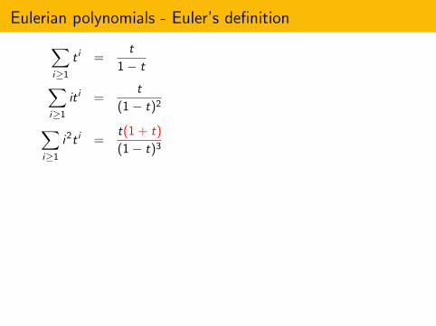
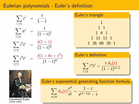
Eulerian polynomials - Euler’s definition
∑i≥1
t i =t
1− t
∑i≥1
it i =t
(1− t)2∑i≥1
i2t i =t(1 + t)
(1− t)3∑i≥1
i3t i =t(1 + 4t + t2)
(1− t)4
Euler’s triangle
11 1
1 4 11 11 11 1
1 26 66 26 1
Euler’s definition∑i≥1
int i =t An(t)
(1− t)n+1
Leonhard Euler(1707-1783)
Euler’s exponential generating function formula∑n≥0
An(t)zn
n!=
1− t
e(t−1)z − t=
(1− t)ez
etz − tez

Eulerian polynomials - Euler’s definition
∑i≥1
t i =t
1− t∑i≥1
it i =t
(1− t)2
∑i≥1
i2t i =t(1 + t)
(1− t)3∑i≥1
i3t i =t(1 + 4t + t2)
(1− t)4
Euler’s triangle
11 1
1 4 11 11 11 1
1 26 66 26 1
Euler’s definition∑i≥1
int i =t An(t)
(1− t)n+1
Leonhard Euler(1707-1783)
Euler’s exponential generating function formula∑n≥0
An(t)zn
n!=
1− t
e(t−1)z − t=
(1− t)ez
etz − tez
Eulerian polynomials - Euler’s definition
∑i≥1
t i =t
1− t∑i≥1
it i =t
(1− t)2∑i≥1
i2t i =t(1 + t)
(1− t)3
∑i≥1
i3t i =t(1 + 4t + t2)
(1− t)4
Euler’s triangle
11 1
1 4 11 11 11 1
1 26 66 26 1
Euler’s definition∑i≥1
int i =t An(t)
(1− t)n+1
Leonhard Euler(1707-1783)
Euler’s exponential generating function formula∑n≥0
An(t)zn
n!=
1− t
e(t−1)z − t=
(1− t)ez
etz − tez

Eulerian polynomials - Euler’s definition
∑i≥1
t i =t
1− t∑i≥1
it i =t
(1− t)2∑i≥1
i2t i =t(1 + t)
(1− t)3∑i≥1
i3t i =t(1 + 4t + t2)
(1− t)4
Euler’s triangle
11 1
1 4 11 11 11 1
1 26 66 26 1
Euler’s definition∑i≥1
int i =t An(t)
(1− t)n+1
Leonhard Euler(1707-1783)
Euler’s exponential generating function formula∑n≥0
An(t)zn
n!=
1− t
e(t−1)z − t=
(1− t)ez
etz − tez
Eulerian polynomials - Euler’s definition
∑i≥1
t i =t
1− t∑i≥1
it i =t
(1− t)2∑i≥1
i2t i =t(1 + t)
(1− t)3∑i≥1
i3t i =t(1 + 4t + t2)
(1− t)4
Euler’s triangle
11 1
1 4 11 11 11 1
1 26 66 26 1
Euler’s definition∑i≥1
int i =t An(t)
(1− t)n+1
Leonhard Euler(1707-1783)
Euler’s exponential generating function formula∑n≥0
An(t)zn
n!=
1− t
e(t−1)z − t
=(1− t)ez
etz − tez

Eulerian polynomials - Euler’s definition
∑i≥1
t i =t
1− t∑i≥1
it i =t
(1− t)2∑i≥1
i2t i =t(1 + t)
(1− t)3∑i≥1
i3t i =t(1 + 4t + t2)
(1− t)4
Euler’s triangle
11 1
1 4 11 11 11 1
1 26 66 26 1
Euler’s definition∑i≥1
int i =t An(t)
(1− t)n+1
Leonhard Euler(1707-1783)
Euler’s exponential generating function formula∑n≥0
An(t)zn
n!=
1− t
e(t−1)z − t=
(1− t)ez
etz − tez

Eulerian polynomials - combinatorial interpretation
For σ ∈ Sn,
Descent set: DES(σ) := {i ∈ [n − 1] : σ(i) > σ(i + 1)}
σ = 3.25.4.1 DES(σ) = {1, 3, 4}Define des(σ) := |DES(σ)|. So
des(32541) = 3
Excedance set: EXC(σ) := {i ∈ [n − 1] : σ(i) > i}
σ = 32541 EXC(σ) = {1, 3}Define exc(σ) := |EXC(σ)|. So
exc(32541) = 2

Eulerian polynomials - combinatorial interpretation
S3 des exc
123 0 0
132 1 1
213 1 1
231 1 2
312 1 1
321 2 1
∑σ∈S3
tdes(σ) = 1+4t+t2
∑σ∈S3
texc(σ) = 1+4t+t2
11 1
1 4 11 11 11 1
1 26 66 26 1
Eulerian polynomial
An(t) =n−1∑j=0
⟨nj
⟩t j =
∑σ∈Sn
tdes(σ) =∑σ∈Sn
texc(σ)
MacMahon (1905) showed equidistribution of des and exc.Carlitz and Riordin (1955) showed these are Eulerian polynomials.
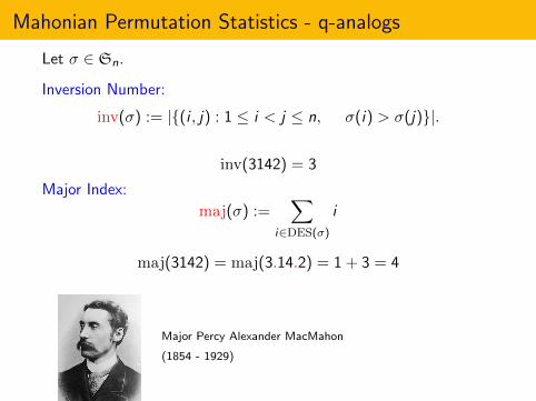
Mahonian Permutation Statistics - q-analogs
Let σ ∈ Sn.
Inversion Number:
inv(σ) := |{(i , j) : 1 ≤ i < j ≤ n, σ(i) > σ(j)}|.
inv(3142) = 3
Major Index:
maj(σ) :=∑
i∈DES(σ)
i
maj(3142) = maj(3.14.2) = 1 + 3 = 4
Major Percy Alexander MacMahon
(1854 - 1929)

Mahonian Permutation Statistics - q-analogs
S3 inv maj
123 0 0
132 1 2
213 1 1
231 2 2
312 2 1
321 3 3
∑σ∈S3
qinv(σ) =∑σ∈S3
qmaj(σ)
= 1 + 2q + 2q2 + q3
= (1 + q + q2)(1 + q)
Theorem (MacMahon 1905)∑σ∈Sn
qinv(σ) =∑σ∈Sn
qmaj(σ) = [n]q!
where [n]q := 1 + q + · · ·+ qn−1 and [n]q! := [n]q[n − 1]q · · · [1]q

q-Eulerian polynomials
Ainv,desn (q, t) :=
∑σ∈Sn
qinv(σ)tdes(σ)
Amaj,desn (q, t) :=
∑σ∈Sn
qmaj(σ)tdes(σ)
Ainv,excn (q, t) :=
∑σ∈Sn
qinv(σ)texc(σ)
Amaj,excn (q, t) :=
∑σ∈Sn
qmaj(σ)texc(σ)
Theorem (MacMahon, 1916; Carlitz, 1954)∑i≥1
[i ]nq t i =tAmaj,des
n (q, t)∏ni=0(1− tqi )

q-Eulerian polynomials
Ainv,desn (q, t) :=
∑σ∈Sn
qinv(σ)tdes(σ)
Amaj,desn (q, t) :=
∑σ∈Sn
qmaj(σ)tdes(σ)
Ainv,excn (q, t) :=
∑σ∈Sn
qinv(σ)texc(σ)
Amaj,excn (q, t) :=
∑σ∈Sn
qmaj(σ)texc(σ)
Theorem (MacMahon, 1916; Carlitz, 1954)∑i≥1
[i ]nq t i =tAmaj,des
n (q, t)∏ni=0(1− tqi )

q-analogs of Euler’s exp. generating function formula
Theorem (Stanley, 1976)∑n≥0
Ainv,desn (q, t)
zn
[n]q!=
1− t
Expq(z(t − 1))− t
where
Expq(z) :=∑n≥0
q(n2)zn
[n]q!
Theorem (Shareshian-W., 2006)∑n≥0
Amaj,excn (q, t)
zn
[n]q!=
(1− tq) expq(z)
expq(ztq)− tq expq(z)
where
expq(z) :=∑n≥0
zn
[n]q!

q-analogs of Euler’s exp. generating function formula
Theorem (Stanley, 1976)∑n≥0
Ainv,desn (q, t)
zn
[n]q!=
1− t
Expq(z(t − 1))− t
where
Expq(z) :=∑n≥0
q(n2)zn
[n]q!
Theorem (Shareshian-W., 2006)∑n≥0
Amaj,excn (q, t)
zn
[n]q!=
(1− tq) expq(z)
expq(ztq)− tq expq(z)
where
expq(z) :=∑n≥0
zn
[n]q!

q-Eulerian polynomials and q-Eulerian numbers
Theorem (Shareshian-W., 2006)∑n≥0
Amaj,excn (q, tq−1)
zn
[n]q!=
(1− t) expq(z)
expq(zt)− t expq(z)
We use symmetric function theory and bijective combinatorics to provethis.
From now on the q-Eulerian polynomials and the q-Eulerian numbers are
An(q, t) := Amaj,excn (q, tq−1) =
∑σ∈Sn
qmaj(σ)−exc(σ)texc(σ)
⟨nj
⟩q
:=∑σ∈Sn
exc(σ)=j
qmaj(σ)−exc(σ)
So the result with Shareshian becomes∑n≥0
An(q, t)zn
[n]q!=
(1− t) expq(z)
expq(zt)− t expq(z)

Palindromicity and unimodality of the q-Eulerian numbers
n\j 0 1 2 3 4
1 1
2 1 1
3 1 2 + q + q2 1
4 1 3 + 2q + 3q2 + 2q3 + q4 3 + 2q + 3q2 + 2q3 + q4 1
5 1 4 + 3q + 5q2 + ... 6 + 6q + 11q2 + ... 4 + 3q + 5q2 + ... 1
Theorem (Shareshian-W., 2006)
The q-Eulerian polynomial An(q, t) =∑n−1
t=0
⟨nj
⟩qt j is
palindromic in the sense that⟨
nj
⟩q
=⟨
nn − 1− j
⟩qfor
0 ≤ j ≤ n−12
q-unimodal in the sense that⟨
nj
⟩q−⟨
nj − 1
⟩q∈ N[q] for
1 ≤ j ≤ n−12

A symmetric function analog of the Eulerian polynomials
Let ω be the involution on the ring of symmetric functionsthat takes the elementary symmetric functions en to thecomplete homogeneous symmetric functions hn.
For a homogeneous symmetric function f (x1, x2, . . . ) ofdegree n with coefficients in ring R, the stable principalspecialization of f is
psq (f (x1, x2, . . . )) = f (1, q, q2, . . . )n∏
i=1
(1− qi ) ∈ R[q].
Let Wn := {w ∈ Zn>0 : wi 6= wi+1 ∀i} (Smirnov words) and let
Wn(x, t) :=∑
w∈Wn
tdes(w) xw1 · · · xwn .
Example: 37572 ∈W5 contributes t2x2x3x5x27 to W5(x, t).

A symmetric function analog of the Eulerian polynomials
Let ω be the involution on the ring of symmetric functionsthat takes the elementary symmetric functions en to thecomplete homogeneous symmetric functions hn.
For a homogeneous symmetric function f (x1, x2, . . . ) ofdegree n with coefficients in ring R, the stable principalspecialization of f is
psq (f (x1, x2, . . . )) = f (1, q, q2, . . . )n∏
i=1
(1− qi ) ∈ R[q].
Let Wn := {w ∈ Zn>0 : wi 6= wi+1 ∀i} (Smirnov words) and let
Wn(x, t) :=∑
w∈Wn
tdes(w) xw1 · · · xwn .
Theorem (Shareshian-W., 2006)
An(q, t) = psq(ωWn(x, t))

Chromatic polynomials
A proper coloring of a graphG = (V ,E ) is a map c : V → Csuch that c(u) 6= c(v) if{u, v} ∈ E .
1
23
4
5
67 8
The chromatic polynomial χG (m) of a graph G is defined to bethe number of proper colorings c : V → C where |C | = m.
V = [n] := {1, . . . , n}E = {{i , i + 1} : i ∈ [n − 1]}χG (m) = m(m − 1)n−1 ∈ Z[m]
1
5
67 8 15 15
23
23
23
35
41 2 3
17 32 17 9
Birkhoff introduced this for planar graphs in 1912 as a means ofproving the four color theorem. Whitney generalized this to allgraphs in 1932.

Stanley’s chromatic symmetric function -1995
1
23
4
5
67 8
77
15 15
23
23
23
35
23
23
Let C (G ) be set of proper colorings c : [n]→ Z>0 of graph G = ([n],E ).
XG (x) :=∑
c∈C(G)
xc(1)xc(2) . . . xc(n)
XG (1, 1, . . . , 1︸ ︷︷ ︸, 0, 0, . . . ) = χG (m)
m
1
5
67 8 15 15
23
23
23
35
41 2 3
17 32 17 9When G is the path with nnodes, XG (x) = Wn(x, 1).

A refinement
1
23
4
5
67 8
77
15 15
23
23
23
35
23
23
Chromatic quasisymmetric function (Shareshian-W., 2011)
XG (x, t) :=∑
c∈C(G)
tdesG (c)xc(1)xc(2) . . . xc(n)
where
desG (c) := |{{i , j} ∈ E (G ) : i < j and c(i) > c(j)}|.
When G is the path with n nodes, XG (x, t) = Wn(x, t) and so
An(q, t) = psq(ωXG (x, t))

When is XG (x, t) symmetric?
Given a collection of n unit intervals I1, . . . , In on R, labeled fromleft to right, form a labeled graph G = ([n],E ), where
E = {{i , j} : Ii ∩ Ij 6= ∅}.
This is called a natural unit interval graph.
Example.
1
5
67 8 15 15
23
23
23
35
41 2 3
17 32 17 9

When is XG (x, t) symmetric?
Examples: Let Gn,r be the graph with vertex set {1, 2, . . . , n} andedge set {{i , j} | 0 < |j − i | ≤ r}.
G4,1 is the path:
1
5
67 8 15 15
23
23
23
35
41 2 3
17 32 17 9
G4,2 is the graph:
1
5
67 8 15 15
23
23
23
35
41 2 3
17 32 17 9
41 2 3
Gn,n−1 is the complete graph Kn.
Theorem (Shareshian-W., 2011)
If G is a natural unit interval graph then XG (x, t) is symmetric in xand palindromic (as a polynomial in t).
XG3,1 = e3 + (e3 + e2,1)t + e3t2
XG4,1 = e4 + (e4 + e3,1 + e2,2)t + (e4 + e3,1 + e2,2)t2 + e4t3

Refinement of Stanley-Stembridge e-positivity conjecture
Let G be a natural unit interval graph.
Conjecture (Shareshian-W., ’11 )
XG (x, t) is e-positive and e-unimodal.
True for
Gn,1 and Gn,r , r ≥ n − 3 (Shareshian-W., 2011)
various infinite classes (Shareshian-W., 2014; Cho-Huh, 2018)
computer verification up to n = 9
Theorem (Shareshian-W., ’14)
XG (x, t) is Schur-positive.
Theorem (Shareshian-W. ’14, Athanasiadis,’15)
ωXG (x, t) is p-positive.
(t = 1 Schur positivity: Haiman, 1993, Gasharov, 1993; t = 1 p-positivity: Stanley forall graphs.)

Specializing ωXGn,r(x, t)
Let 1 ≤ r ≤ n − 1. Our refinement of the Stanley-Stembridge conjectureimplies: psq(ωXGn,r (x, t)) is palindromic and q-unimodal.
Let A(r)n (q, t) :=
∑σ∈Sn
qmaj>r (σ)t inv≤r (σ) where
inv≤r (σ) := |{(i , j) : 1 ≤ i < j ≤ n, 0 < σ(i)− σ(j)≤ r}|DES>r (σ) := {i ∈ [n − 1] : σ(i)− σ(i + 1)> r}maj>r (σ) :=
∑i∈DES>r
i
Theorem (Shareshian-W., 2011)
psq(ωXGn,r (x, t)) = A(r)n (q, t)
Consequently A(1)n (q, t) = An(q, t).
Proof involves quasisymmetric function theory.

A(r)n (q, t) :=
∑σ∈Sn
qmaj>r (σ)t inv≤r (σ)
Exercise (Stanley EC1, 1.50 f): Prove that∑
σ∈Snt inv≤r (σ) is
palindromic and unimodal.Solution:
Theorem (De Mari and Shayman - 1988)
Let Hn,r be the type An−1 regular semisimple Hessenberg varietyof degree r . Then
∑σ∈Sn
t inv≤r (σ) =
d(n,r)∑j=0
dimH2j(Hn,r )t j
Consequently by the hard Lefschetz theorem,∑
σ∈Snt inv≤r (σ) is
palindromic and unimodal.
Stanley: Is there a more elementary proof of unimodality?Shareshian-W.: Can we find a q-analog or a symmetric functionanalog?

A(r)n (q, t) :=
∑σ∈Sn
qmaj>r (σ)t inv≤r (σ)
Exercise (Stanley EC1, 1.50 f): Prove that∑
σ∈Snt inv≤r (σ) is
palindromic and unimodal.Solution:
Theorem (De Mari and Shayman - 1988)
Let Hn,r be the type An−1 regular semisimple Hessenberg varietyof degree r . Then
∑σ∈Sn
t inv≤r (σ) =
d(n,r)∑j=0
dimH2j(Hn,r )t j
Consequently by the hard Lefschetz theorem,∑
σ∈Snt inv≤r (σ) is
palindromic and unimodal.
Stanley: Is there a more elementary proof of unimodality?
Shareshian-W.: Can we find a q-analog or a symmetric functionanalog?

A(r)n (q, t) :=
∑σ∈Sn
qmaj>r (σ)t inv≤r (σ)
Exercise (Stanley EC1, 1.50 f): Prove that∑
σ∈Snt inv≤r (σ) is
palindromic and unimodal.Solution:
Theorem (De Mari and Shayman - 1988)
Let Hn,r be the type An−1 regular semisimple Hessenberg varietyof degree r . Then
∑σ∈Sn
t inv≤r (σ) =
d(n,r)∑j=0
dimH2j(Hn,r )t j
Consequently by the hard Lefschetz theorem,∑
σ∈Snt inv≤r (σ) is
palindromic and unimodal.
Stanley: Is there a more elementary proof of unimodality?Shareshian-W.: Can we find a q-analog or a symmetric functionanalog?

Symmetric function analog
The Frobenius characteristic is a linear mapch : {virtual Sn-modules} −→ Λn,
where Λn is the vector space of homogeneous symmetric functionsof degree n.
The image of the set of (actual) Sn-modules equals the set ofSchur-positive symmetric functions of degree n.
We need a representation of Sn on H2j(Hn,r ) whose Frobeniuscharacteristic is the coefficient of t j in ωXGn,r (x, t). It also has tocommute with the hard Lefshetz map.
H2j(Hn,r ) 7−→ch ωXGn,r (x, t)|t j 7−→psq
A(r)n (q, t)|t j
Tymoczko (2008) used GKM theory (Goresky, Kottwitz,MacPherson) to obtain a representation of Sn on eachcohomology.
Does this representation work for us?

First - more general Hessenberg variety
De Mari, Procesi, Shayman (1992) extended the notion ofsemisimple Hessenberg variety so that Hm is defined for eachsequence m = (m1 ≤ · · · ≤ mn) of integers satisfying1 ≤ i ≤ mi ≤ n. (Call these Hessenberg sequences.)
There is a bijection between natural unit interval graphs andHessenberg seqences. Let
HG := Hm(G)
where m(G ) is the Hessenberg sequence associated withnatural unit interval graph G .

Symmetric function analog
Conjecture (Shareshian and W., 2011)
Let chH2j(HG ) be the Frobenius characteristic of Tymoczko’srepresentation of Sn on H2j(HG ). Then
ωXG (x, t) =∑j≥0
chH2j(HG )t j .
Consequenlty, by the Hard Lefschetz Theorem ωXG (x, t) is Schurunimodal.
If this conjecture is true then our refinement of theStanley-Stembridge e-positivity conjecture is equivalent to:
Conjecture
Tymoczko’s representation of Sn on H2j(HG ) is a permutationrepresentation for which each point stabilizer is a Young subgroup.

Hessenberg varieties (De Mari-Shayman (1988), De Mari-Procesi-Shayman (1992))
Let Fn be the set of all flags of subspaces of Cn
F : F1 ⊂ F2 ⊂ · · · ⊂ Fn = Cn
where dimFi = i .
The type A regular semisimple Hessenberg variety associated withnatural unit interval graph G is
HG := {F ∈ Fn | DFi ⊆ Fmi (G) ∀i ∈ [n]},
where
D is the n × n diagonal matrix whose diagonal entries are1, 2, . . . , n
m(G ) = (m1(G ),m2(G ), . . . ,mn(G )) is the Hessenbergsequence associated with G .

GKM theory and moment graphs
Goresky, Kottwitz, MacPherson (1998): Construction ofequivariant cohomology ring of smooth complex projective varietieswith a torus action. From this, one gets ordinary cohomology ring.
The group T of nonsingular n × n diagonal matrices acts on
HG := {F ∈ Fn | DFi ⊆ Fmi (G) ∀i ∈ [n]}.by left multiplication.
Moment graph: graph whose vertices are T -fixed points and whoseedges are one-dimensional orbits.
Fixed points of the torus action:
Fσ : 〈eσ(1)〉 ⊂ 〈eσ(1), eσ(2)〉 ⊂ · · · ⊂ 〈eσ(1), . . . , eσ(n)〉where σ is a permutation.So the vertices of the moment graph can be represented bypermutations.

Combinatorial description of the moment graph
Let G = ([n],E ) be a natural unit interval graph. The moment graphΓ(G ) for the Hessenberg variety HG has vertex set Sn and edge set
{{σ, σ(i , j)} : σ ∈ Sn and {i , j} ∈ E}.
Example: n = 3.
123
213
231
132
312
321
123
213
231
132
312
321
123
213
231
132
312
321
123
213
231
132
312
321
(2,3) (1,3)(1,2)Color coded edge labels:
1 2 3 1 2 3 1 2 3
1 2
3

The equivariant cohomology ring H∗T (HG )
H∗T (HG ) is isomorphic to a subring of Rn :=∏σ∈Sn
C[t1, . . . , tn].
For p ∈ Rn, let pσ(t1, . . . , tn) ∈ C[t1, . . . , tn] denote theσ-component of p, where σ ∈ Sn.
(2,3) (1,3)(1,2)Color coded edge labels:
1 2 3
123
213
231
132
312
321 0
0
0
0
t1 � t2
t3 � t2
�( )
p ∈ Rn satisfies the edge condition forthe moment graph ΓG if for all edges{σ, τ} of Γ(G ) with label (i , j), thepolynomial
pσ(t1, . . . , tn)− pτ (t1, . . . , tn)
is divisible by ti − tj .
H∗T (HG ) is isomorphic to the subring of Rn whose elements satisfythe edge condition for ΓG .

Tymoczko’s representation
σ ∈ Sn acts on p ∈ H∗T (HG ) by
(σp)τ (t1, . . . , tn) = pσ−1τ (tσ(1), . . . , tσ(n))
(2,3) (1,3)(1,2)Color coded edge labels:
1 2 3
123
213
231
132
312
321 0
0
0
0
t1 � t2
t3 � t2
�( )
H∗(HG ) ∼= H∗T (HG )/〈t1, . . . , tn〉H∗T (HG )
The representation of Sn on H∗T (HG ) induces a representation onthe graded ring H∗(HG ).The hard Lefschetz map commutes with the action of Sn.

Tymoczko’s representation
σ ∈ Sn acts on p ∈ H∗T (HG ) by
(σp)τ (t1, . . . , tn) = pσ−1τ (tσ(1), . . . , tσ(n))
(2,3) (1,3)(1,2)Color coded edge labels:
1 2 3
123
213
231
132
312
321 0
0
0
0
t1 � t2
t3 � t2
�( )
(1, 2)
1 2 3
123
213
231
132
312
321
0
0
0
0
�( )
t2 � t1
t3 � t1
H∗(HG ) ∼= H∗T (HG )/〈t1, . . . , tn〉H∗T (HG )
The representation of Sn on H∗T (HG ) induces a representation onthe graded ring H∗(HG ).The hard Lefschetz map commutes with the action of Sn.

Consequences of our conjecture
Let G be a natural unit interval graph. The conjecture
ωXG (x, t) =∑j≥0
chH2j(HG )t j
has the following consequences..Combinatorial consequences:
XG (x, t) is Schur-positive and Schur-unimodal.
Generalized q-Eulerian polynomials A(r)n (q, t) are q-unimodal.
Algebro-geometric consequences:
Multiplicity of irreducibles in Tymoczko’s representation canbe obtained from our expansion of XG (x, t) in Schur basis.
Character of Tymoczko’s representation can be obtained fromour expansion of XG (x, t) in power-sum basis.
So our conjecture is a two-way bridge between combinatorics andalgebraic geometry.
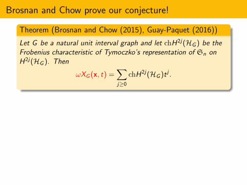
Brosnan and Chow prove our conjecture!
Theorem (Brosnan and Chow (2015), Guay-Paquet (2016))
Let G be a natural unit interval graph and let chH2j(HG ) be theFrobenius characteristic of Tymoczko’s representation of Sn onH2j(HG ). Then
ωXG (x, t) =∑j≥0
chH2j(HG )t j .
Brosnan and Chow reduce the problem of computingTymaczko’s representation of Sn on regular semisimpleHessenberg varieties to that of computing the Betti numbersof regular (but not nec. semisimple) Hessenberg varieties. Todo this they use results from the theory of local systems andperverse sheaves. In particular they use the local invariantcycle theorem of Beilinson-Bernstein-DeligneGuay-Paquet introduces a new Hopf algebra on labeled graphsto recursivley decompose the regular semisimple Hessenbergvarieties.

Other recently discovered connections with XG (x, t)
Hecke algebra characters evaluated at Kazhdan-Lusztig basiselements: Clearman-Hyatt-Shelton-Skandera (2015). This is at-analog of work of Haiman (1993).
Macdonald polynomials: Haglund-Wilson (’17).
LLT polynomials: Carlsson-Mellit (’15), Haglund-Wilson (’17).

Other symmetric XG (x, t)
Extension of p-positivity result.
Theorem (Ellzey (2016))
If G is a labeled graph for which XG (x, t) is symmetric thenωXG (x, t) is p-positive.
Quasisymmetric power-sum functions: Ballantine, Daugherty,Hicks, Mason, and Niese (2017)
Theorem (Alexandersson-Sulzgruber (2018))
For any labeled graph G , the chromatic quasisymmetric functionωXG (x, t) is quasisymmetric p-positive.
The proof uses Ellzey’s techniques.

Other symmetric XG (x, t)
12
3
45
6
7
8
C8 =not a unit interval graph
Theorem (Stanley (1995))
XCn(x) is e-positive for all n ≥ 2.
Theorem (Ellzey-W. (2018))
XCn(x, t) is e-positive for all n ≥ 2.
Are there any other labeled connected graphs whose chromaticquasisymmetric function is symmetric besides for the natural unitinterval graphs and the naturally labeled cycle?
Ellzey, 2018 UM Ph.D thesis: directed graph version.


![Chromatic polynomials and order ideals of monomials€¦ · · 2015-07-29found to be the quickest form of the chromatic polynomial to calculate [32]. What ... to explicitly determine](https://static.fdocuments.net/doc/165x107/5ac924a87f8b9aa3298cb945/chromatic-polynomials-and-order-ideals-of-monomials-2015-07-29found-to-be-the.jpg)