i

From Electrode Materials to Dynamic Models of Li-ion Cells

An Undergraduate Honors Thesis

Submitted to the Department of Mechanical Engineering

The Ohio State University

In Partial Fulfillment of the Requirements

for Graduation with Distinction in Mechanical Engineering

Bo Jiang

Spring, 2013

Dr. G Rizzoni, Advisor

ii

Abstract

Batteries play a fundamental role in electric vehicles, and help to reduce the

environmental impact associated with fossil fuels. Li-ion battery is a promising candidate for

vehicles due to its specific energy. This project is focused on experimental characterization

and modeling of Li-ion batteries, and the objectives are to analyze battery aging at an

electrode level and to better predict battery performance.

The project consists of fabricating half cells of Lithium Iron Phosphate coin cells from

unaged and batteries aged under different conditions, and measuring relevant parameters

including capacity, state of charge, impedance, and open-circuit voltage.

An equivalent circuit was developed from charging and discharging profile and

impedance measurements with parameters calibrated to model the cell behavior. The

governing equation of the non-linear system can be approximated by a Pade function with

second-order numerator and denominator. The disadvantage of Pade function is that

coefficients in the function do not have a physical meaning. The simple equivalent circuit and

the linear Pade function will allow fast calculations during design and prediction, and

improve the efficiency of predictive maintenance.

iii

ACKNOWLEDGEMENTS

I would first and foremost like to thank Dr. Giorgio Rizzoni. He gave me a last minute

chance for undergraduate honors research and introduced me to this project. He was not only

a knowledgeable professor, but also a caring and encouraging advisor. Busy as he is, he

always takes time to guide me. Outside of this project, he tries to give me the best graduate

school research and scholarship opportunities. I always feel lucky to have him as my advisor.

A huge thank you goes to Dr. Shrikant Nagpure. He taught me all the experimental

procedures, explained details of the projects, and worked during weekends just to keep my

project moving forward.

I greatly appreciate Mr. Alex Bartlett’s help. He has being so generous with his time in

replying emails and meeting. He passed down his experiences and set up the outstanding

example for me to follow.

iv

Table of Contents:

Abstracts ...............................................................................................................................ii

Acknowledgements ..............................................................................................................iii

Table of Contents .................................................................................................................iv

List of Figures .......................................................................................................................vi

List of Tables ........................................................................................................................viii

Chapter 1: Introduction ......................................................................................................1

1.1 Motivation for Li-ion battery aging research ............................................................1

1.2 Objectives .................................................................................................................3

1.3 Overview of thesis ....................................................................................................4

Chapter 2: Background………………………………………………………………….. 5

2.1 Circuit models of electrochemical processes ............................................................5

2.2 Advantages of equivalent circuit models ..................................................................6

2.3 Methods of developing equivalent circuit models ....................................................10

2.4 Related concepts .......................................................................................................11

Chapter 3: Experimental Design ........................................................................................12

3.1 Overview of design ...................................................................................................12

3.2 Procedure of fabricating coin cells and collecting data ............................................13

3.2.1 Experimental specimen groups .......................................................................13

3.2.2 Coin cell fabrication procedure .......................................................................14

3.2.3 Data collection procedure ...............................................................................18

Chapter 4: Results and Discussion .....................................................................................22

4.1 Experimental results .................................................................................................22

4.2 One-element equivalent circuit model .....................................................................25

4.3 One-element equivalent circuit impedance parameter calibration ............................28

4.3.1 Gamry automatic fitting ..................................................................................28

v

4.3.2 Pade approximation ........................................................................................31

4.3.3 Least square fitting with Pade function ..........................................................33

4.4 Two-element equivalent circuit model ....................................................................36

Chapter 5: Conclusion and Recommendation for Future Work ....................................40

5.1 Conclusion ................................................................................................................40

5.2 Recommendation for future work .............................................................................41

References .............................................................................................................................42

vi

List of Figures

Figure 1: Typical Capacity Curves of a Battery .............................................................................. 2

Figure 2: An Equivalent Circuit Model Used to Simulate LiB Performance [11] .......................... 7

Figure 3: Schematic diagram of the Rint model [13] ...................................................................... 7

Figure 4: Schematic diagram for the Thevenin model [13] ............................................................ 8

Figure 5: Schematic diagram of the PNGV model [13] .................................................................. 9

Figure 6: Schematic diagram of the DP model [13] ..................................................................... 10

Figure 7: Components of a coin cell [] ......................................................................................... 15

Figure 8: VWR symphonyTM

Vacuum Oven [] ............................................................................ 16

Figure 9: LABstar glove box ........................................................................................................ 16

Figure 10: Chamber of LABstar glove box [] ............................................................................... 17

Figure 11: Compact Hydraulic Crimping Machine (MSK-110) [] ............................................... 18

Figure 12: Charging profile for C7 cathode as working electrode ................................................ 22

Figure 13: Discharging profile for C7 cathode as working electrode ........................................... 23

Figure 14: Complete EIS curves for C7 cathode .......................................................................... 24

Figure 15: Equivalent circuit model with ideal elements .............................................................. 25

Figure 16: Ideal and real EIS curve .............................................................................................. 26

Figure 17: Modified circuit model with constant phase element .................................................. 27

Figure 18: EIS curves for C7 cathode above 1 Hz ........................................................................ 28

Figure 19: Experimental and Gamry fitted EIS curve of C7 cathode at 20% during charging ..... 30

Figure 20: Experimental and Gamry fitted Bode plot of C7 cathode at 20% during charging ..... 30

Figure 21: Nyquist plot of nonlinear and Pade function ............................................................... 33

Figure 22: Nyquist plot of Nonlinear and Pade function from least square fitting ....................... 34

Figure 23: Bode plot of Nonlinear and Pade function from least square fitting ........................... 35

vii

Figure 24: Nyquist plot of nonlinear and Pade functions ............................................................. 35

Figure 25: Bode plot of nonlinear and Pade function ................................................................... 36

Figure 26: Step response of Pade function .................................................................................... 36

Figure 27: Two-element equivalent circuit model ........................................................................ 37

Figure 28: Experimental and Gamry fitted EIS curve of C7 cathode at 20% during charging ..... 37

Figure 29: Experimental and Gamry fitted Bode curve of C7 cathode at 20% during charging .. 38

viii

List of Table

Table 1: Matrix of samples for coin cell fabrication based on aging ............................................ 13

Table 2: Sample for coin cell testing ............................................................................................ 14

Table 3: Testing protocol for discharging and charging ............................................................... 19

Table 4: Values of parameters for one-element circuit from Gamry curve fitting........................ 29

Table 5: Parameters for two-element circuit from Gamry curve fitting ....................................... 38

1

Chapter 1: Introduction

1.1 Motivation for Li-ion battery aging research

The issues related to fossil fuels, including the limited amount, fluctuating prices, and

associated environmental problems, are driving people’s attention to more efficient usage of

fossil fuels. The last two decades have witnessed a great advancement in mass production of

Hybrid, Plug-in Hybrid, and Electric Vehicles (HEV, PHEV, and EV). Toyota launched their

first generation Prius in Japan in 1997 [1]; the Honda CR-Z made its debut in 2008 in Detroit

[2]; the Chevy Volt was introduced in 2007 [3]. They adopt an electric propulsion system to

achieve a better fuel economy and reduce emissions.

Rechargeable batteries play a fundamental role in HEV, PHEV and EV. In a hybrid

electric vehicle, a battery pack is added to provide propulsion along with the internal

combustion engine, while in an EV the battery pack provides all the power. Based on the

design of the power train control system, the battery pack is charged and discharged with

variable current rates during vehicle operation, posing different requirements and challenges

to the battery pack. There has been a significant increase in interest in lithium ion batteries

for HEVs due to the demand for high specific energy and specific power [4]. Specific energy

describes the nominal battery energy per unit mass, and determines the battery weight to

achieve a desired electric range. Specific power is the maximum power available per unit

mass, and determines battery weight for a given performance target. [5] The high energy and

power density of lithium ion batteries allows the development of lighter vehicles for a given

2

vehicle range and performance. Of the many materials tested as cathode materials, LiFePO4

(LFP) is a promising candidate. LFP is environmental friendly, inexpensive, and abundant,

and LFP material features large capacity, good thermal stability, and little hygroscopicity. [4]

In this project, LFP is employed as the cathode material.

As a cell is repeatedly charged and discharged throughout their life, the capacity and

power capabilities of the cell degrade, a phenomenon known as aging. Specifically the

battery capacity drops after a sufficient number of cycles, and the time a fully charged battery

can provide electric power is shortened. The battery voltage also drops more quickly as the

battery discharges as a consequence of aging, which has a more significant effect for high

current applications. Figure 1 shows typical capacity curves of a battery, with voltage on the

vertical axis and time on the horizontal axis. From the figure, it is clear that the capacity

diminishes and voltage drops faster as the battery ages.

Figure 1: Typical Capacity Curves of a Battery

A battery consists of two electrodes, anode and cathode, separated by an insulating

separator and electrolyte. The mechanisms for the aging effect are currently not well

3

understood; although studies have shown aging is highly dependent on the electrode material,

electrolyte, and conditions in which the battery is used [6]. It is generally believed that

lithium deposition, electrolyte decomposition, active material dissolution, phase transition

inside the insertion electrode materials, and further passive film formation on the electrode

and current collectors, all contribute to different degrees of battery aging [7]. Specifically the

aging mechanism is different at each electrode. However if only the capacity and power fade

of the complete cell are analyzed, the contributions of each electrode cannot be easily

discerned from the overall aging. By fabricating coin cells made from each electrode of a

deconstructed aged cell, the aging contributions of each electrode can by analyzed separately.

With an understanding of the changes experienced by each electrode, may gain insight into

the principles behind battery aging, and be able to better predict battery performance. This

provides valuable insight in the relationship between the material degradation and system

level metrics such as capacity and internal resistance of the cell.

1.2 Objectives

This research project was carried out at the battery aging lab at the Center for

Automotive Research. The objectives of the project are listed below.

To analyze battery aging at an electrode level and to better predict battery

performance and improve the efficiency of predictive maintenance;

4

To fabricate half cells of Lithium Iron Phosphate coin cells using anode and cathode

materials harvested from different locations of new and aged batteries to study the

contribution of aging at each electrode to the overall battery aging;

To cycle coin cells, and to measure relevant parameters including capacity, state of

charge, impedance, and open-circuit voltage to understand the changes experienced

by parts of each individual electrode during cycling;

To develop and calibrate separate equivalent circuits for the cathode and anode, with

parameters that are functions of temperature, state of charge, location on an electrode,

and other aging dependent factors to provide a simple tool for predicting battery

performance.

1.3 Overview of thesis

This thesis has 5 chapters. Chapter 2 introduces background. Chapter 3 explains the

experimental setup and design. Chapter 4 includes results and discussions. Chapter 5

summarizes the conclusions. Chapter 6 provides recommendation for future work.

5

Chapter 2: Background

2.1 Circuit models of electrochemical processes

In general a battery does not operate ideally; it involves complicated electrochemical

components and processes, and therefore has an internal impedance. There are several

physical processes that can cause resistive and energy storage effects in a battery. Most

generally, resistive and capacitive behaviors dominate the response of a battery. We first

focus on the internal resistance. First of all, electrolyte solution resistance is a significant part

of internal impedance of battery. Whenever electrons and charged particles traverse the

electrolyte, they face a resistance which depends on the conductivity of the electrolyte and

the distance between the electrons. Unfortunately, most cells do not have uniform current

distribution through a defined electrolyte area, and determination of the resistance requires

specifying the current path and the geometry of electrolyte. Second, as the battery charges

and discharges, the potential of the two electrodes may shift, a phenomenon called

polarization. Polarization can generate current through an electrochemical reaction at the

electrode surface and introduce a polarization resistance. Also there is a resistance associated

with charge transfer. Finally, there is an ohmic resistance as the current travels through the

electrode matrix and current collector. [8]

A second phenomenon that is necessary to model the behavior of a battery is

capacitance. In general, capacitance results from charge separation. Electrochemical

reactions occur at surfaces, and the interface between electrode and electrolyte accumulate

6

opposite charges to form a double layer, which acts like a capacitance.[9] In addition to

capacitive effects, one also encounters more complex behavior caused, for example by the

phenomenon of diffusion, which cannot be easily explained as a resistive or capacitive

behavior. Diffusion can be represented by a so-called Warburg element [10]. Further, the

impedance of an electrochemical cell may sometimes appear to follow and inductive behavior,

and may require an inductor circuit model to represent its response. [11]

2.2 Advantages of equivalent circuit models

Accounting for the detailed processes of the electrochemical mechanism inside the

battery is a lengthy and complicated process, which results in partial differential equations of

considerable complexity if modeled from first principles. As an alternative, equivalent circuit

modeling is a popular approach to study batteries because it greatly simplifies the modeling

process and reduces computational efforts. The approach only requires identifying relatively

few parameters and successfully simulates the input-output behavior of a battery. [12]

The equivalent circuit model (ECM) method has been amply described in the

literature. Liaw provided some concepts and techniques of ECM. [12] An ECM may have

three major components: a static part simulating the thermodynamic properties of

electrochemical processes in battery, a dynamic part representing the kinetics of the cell

internal impedance, and a source or load for charge and discharge regimes. [12] Such a

7

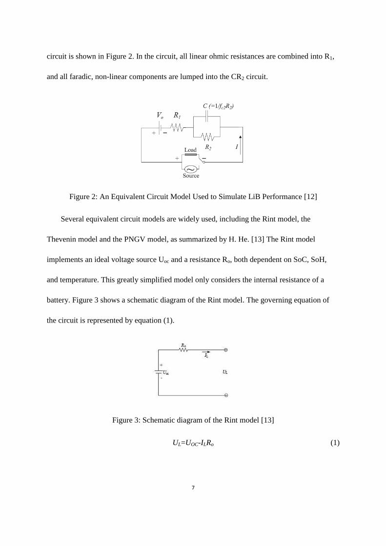
circuit is shown in Figure 2. In the circuit, all linear ohmic resistances are combined into R1,

and all faradic, non-linear components are lumped into the CR2 circuit.

Figure 2: An Equivalent Circuit Model Used to Simulate LiB Performance [12]

Several equivalent circuit models are widely used, including the Rint model, the

Thevenin model and the PNGV model, as summarized by H. He. [13] The Rint model

implements an ideal voltage source Uoc and a resistance Ro, both dependent on SoC, SoH,

and temperature. This greatly simplified model only considers the internal resistance of a

battery. Figure 3 shows a schematic diagram of the Rint model. The governing equation of

the circuit is represented by equation (1).

Figure 3: Schematic diagram of the Rint model [13]

UL=UOC-ILRo (1)

8

The Thevenin model adds to the Rint model a parallel RC circuit in series with Ro,

describing the dynamic characteristics of the battery. Figure 4 shows a schematic diagram of

Thevenin model. The system is governed by equations (2) and (3), where UOC stands for

open-circuit voltage, Ro and RTH stand for internal resistance and polarization resistance

respectively, CTH is the equivalent capacitance, and ITH is the outflow current of CTH [13].

Figure 4: Schematic diagram for the Thevenin model [13]

TH

L

THTH

THTH

C

I

CR

UU (2)

oLTHOCL RIUUU (3)

The PNGV model adds a capacitor to the Thevenin model to describe the changing of

open circuit voltage generated by the time accumulation of load current, as shown in Figure 5.

Ud and UPN are the voltages across capacitors 1/U’OC and CPN respectively, and IPN is the

outflow current of CPN [13]. The system behavior is described by equation (4) (5) and (6).

9

Figure 5: Schematic diagram of the PNGV model [13]

LOCd IUU (4)

PN

L

PNPN

PN

PNC

I

CR

UU

(5)

oLPNdOCL RIUUUU (6)

The Thevenin circuit approximately models the polarization of a lithium-ion power

battery, but cannot accurately capture the difference between concentration polarization and

electrochemical polarization at the end of charge and discharge. To refine the polarization

simulation, the Dual Polarization (DP) model adds one more RC circuit to the Thevenin

model, as shown in Figure 6 [13]. The equivalent circuit that will be used in this thesis is

mainly based on the DP model. The electrical behavior of the DP model can be described by

equations (7) (8) and (9). Capacitors Cpa and Cpc are used to characterize the transient

response due to electrochemical and concentration polarization, respectively. Upa and Upc are

the voltages across Cpa and Cpc respectively. Ipa and Ipc are outflow currents of Cpa and Cpc ,

respectively [13].

10

Figure 6: Schematic diagram of the DP model [13]

pa

L

papa

PNpa

C

I

CR

UU

(7)

pc

L

pcpc

pc

pcC

I

CR

UU

(8)

oLpcpaOCL RIUUUU (9)

2.3 Methods of developing equivalent circuit models

Electrochemical Impedance Spectroscopy (EIS) is the main tool used to identify the

parameters of an equivalent circuit. EIS is a frequency domain analysis method that generates

the Nyquist plot of the cell impedance. EIS is a method based on measuring the sinusoidal

frequency response of the cell by imposing a small signal sinusoidal current of variable

frequency to the cell, and measuring the resulting voltage response. [10] This analysis is

conducted over a broad range of frequencies that can be as low as 0.001 Hz and as high as

100,000 Hz. The results are usually displayed in the form of a Nyquist plot. In a Nyquist plot,

the real part of the cell impedance is plotted on the x-axis and the imaginary part on the y-

11

axis. One drawback of Nyquist plot is that the frequency cannot be seen from the plot.

Conventionally EIS has been used to study kinetics in an electrochemical system. Analyses of

complex impedance data rely on employing an equivalent circuit to simulate cell performance

and behavior, with a series of circuit elements that represent the electrochemical system. [11]

2.4 Related concepts

A few concepts are important in the ECM method. State of charge (SOC) refers to the

present available battery capacity as a percentage of maximum capacity. Depth of discharge

(DOD) refers to the discharged battery capacity as a percentage of maximum capacity, equals

to 1-SOC. There are different concepts related to voltages. Open-circuit voltage is the voltage

between battery terminals at equilibrium when no load is applied, and is a function of the

state of charge. Terminal voltage is the voltage between battery terminals with load applied,

and depends on SOC as well as charge/discharge current. Current rate is a measure of the

discharge current relative to its maximum capacity. 1C rate refers to the current at which the

battery will fully discharge in one hour. 2C is, therefore, twice the current. [5] Higher

discharging current rate appears to accelerate battery aging. According to the study of

capacity fade of Sony US 18650 Li-ion batteries cycled using different discharge rates at

ambient temperature, the capacity loss after 300 cycles at 2C and 3C discharge rates were

estimated to be 13.2% and 16.9% of the initial capacity, while the capacity loss was only 9.5%

at 1C [7].

12

Chapter 3: Experimental Design

3.1 Overview of design

The first stage of this project is fabrication of coin cells using the anode and cathode

material harvested from unaged batteries and batteries aged with different current rates. The

coin cells are fabricated inside a glove box with a controlled Argon atmosphere. The batteries

employ lithium iron phosphate (LFP) as the cathode material and lithium graphite as the

anode material. Working electrode designates the electrode being studied, and reference

electrode is an experimental reference point for potential measurements. [14] When testing

the cathode, the cathode from unaged and aged batteries is used for the working electrode and

unaged lithium material is used for reference electrode. When testing the anode, the anode

from unaged and aged batteries is used for the working electrode, and unaged lithium

material is used for the reference electrode.

Experimental data were collected from the fabricated cell. Each coin cell was subjected

to a multi-rate capacity test and electrochemical impedance test (EIS). The data collected

with these tests will help in comparing the capacity, impedance, and open circuit voltage of

the electrodes harvested from unaged and aged cells. Once enough experimental data is

generated, the next step is to develop an equivalent circuit model for the anode and cathode

using Echem Analyst. Echem Analyst is able to calculate unknown parameters to fit

experimental data given a pre-determined model. A model structure is first chosen and

13

calibrated by adjusting the model parameters until the simulated results fit the experimental

ones. The model structure itself is revised if it cannot accurately capture the cell dynamics.

3.2 Procedure of fabricating coin cells and collecting data

3.2.1 Experimental specimen groups

Current rate has significant effect on the rate of aging. [7] To compare the effect of

different C-rates on aging, the electrode materials are harvested from unaged batteries and

batteries aged with different C-rates. The cells are named by CA-B-D, where A represents the

C-rate the battery was aged at, B represents the campaign and D is the SOC setting for that

campaign. For modes of campaign, 1 stands for Electric Vehicle (EV), 2 stands for PHEV

(Plug-In Hybrid Electric Vehicle), and 3 represents Hybrid Electric Vehicle (HEV). The

electrodes of a battery are rolled in application, and different locations are expected to

experience different reactions and different degree of aging. To study the variation between

different locations, each battery electrode is divided into 5 sections, and four coin cells are

fabricated from electrode material from each section. Location 1 is closest to the periphery of

the cylindrical battery electrode, and Location 5 is closest to the center of the cylindrical

battery. The table below summarizes the different conditions under which each specimen was

aged.

Table 1: Matrix of samples for coin cell fabrication based on aging

Cells C-rate Campaign Location

14

C0 Unaged Unaged 1,2,3,4,5

C2-1-1 2 EV 1,2,3,4,5

C4-1-1 4 EV 1,2,3,4,5

C7-3-1 ~7 HEV 1,2,3,4,5

For the purpose of comparing the anode and cathode from unaged batteries and batteries

aged with three different C-rates and variations at five locations along each electrode, a large

number of coin cells should be fabricated and tested. Due to the time constraint of my project,

only one cell was fabricated and tested. Table 2 summarizes the sample tested in this project.

Table 2: Sample for coin cell testing

Coin Cell C-rate Campaign Electrode Location

1 ~7 HEV Cathode 3

3.2.2 Coin cell fabrication procedure

As shown in Figure 7, the materials used to assemble the coin cells include a lithium

reference electrode, a cathode or anode, a spacer, a spring, and coin cell casings. The spacer

is made from stainless steel and used to provide an electrical connection from the electrode to

the case. A thin layer of polymer plastic is used as the separator. A ring-shaped spring is

placed between the casing and the spacer to exert pressure on the components, press them

together and hold them in place.

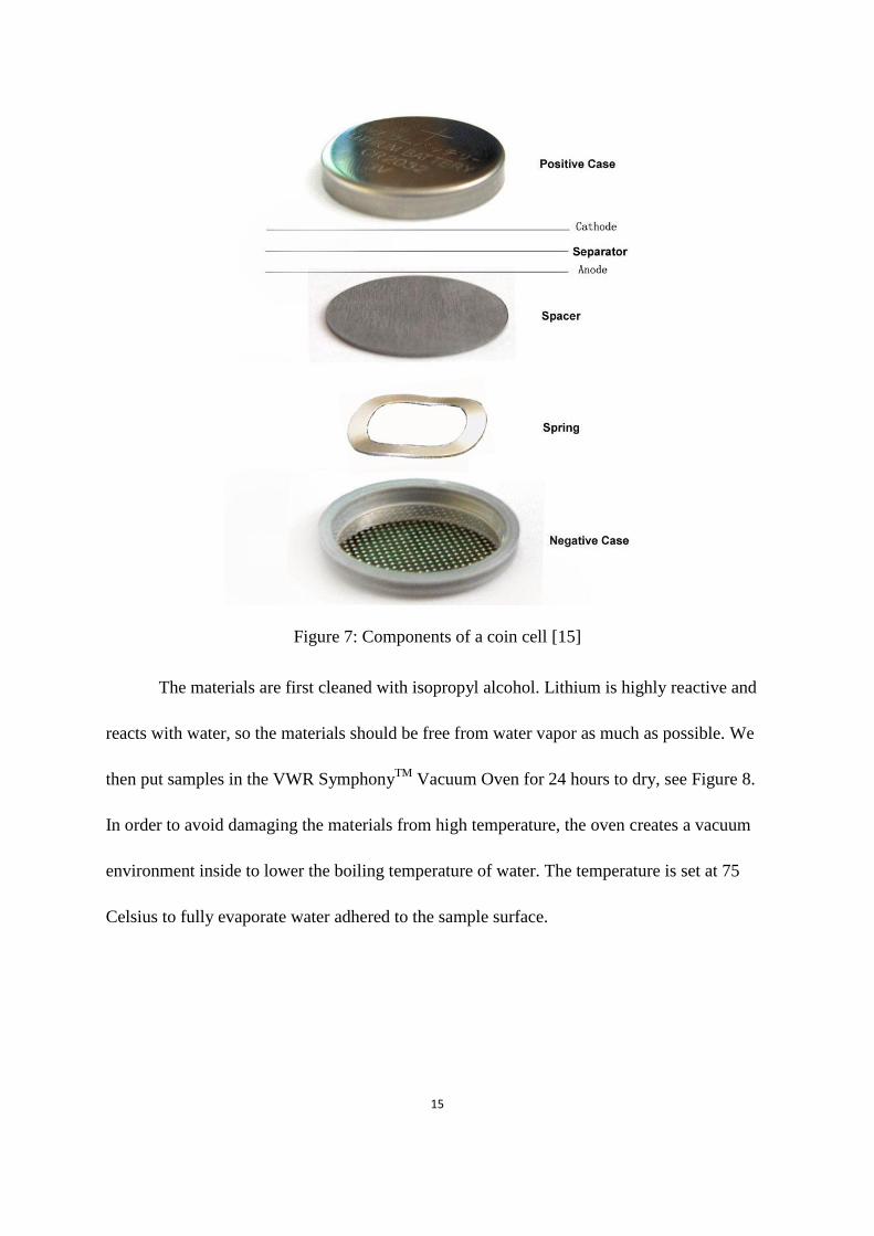
15

Figure 7: Components of a coin cell [15]

The materials are first cleaned with isopropyl alcohol. Lithium is highly reactive and

reacts with water, so the materials should be free from water vapor as much as possible. We

then put samples in the VWR SymphonyTM

Vacuum Oven for 24 hours to dry, see Figure 8.

In order to avoid damaging the materials from high temperature, the oven creates a vacuum

environment inside to lower the boiling temperature of water. The temperature is set at 75

Celsius to fully evaporate water adhered to the sample surface.

16

Figure 8: VWR SymphonyTM

Vacuum Oven [16]

The materials are then transferred to a LABstar glove box after drying, see Figure 9.

The whole assemble process is performed in the glove box in an Argon environment mostly

free from oxygen and water. The glove box is constantly monitored by a control panel, and

the gage pressure is kept at 2-9 mBar, and the concentration of oxygen and vapor is kept

under 5 ppm and 1 ppm respectively. The notation ppm stands for parts-per-million, and is

used to describe the concentration of extremely dilute solutions. When the concentrations of

water and oxygen are above their limits, the gas inside will be pumped out while Argon will

be pumped into the glove box until the concentrations drop below the limits.

Figure 9: LABstar glove box

17

When materials and tools are being transferred, they are first placed in the chamber at

the side of the glove box, as in Figure10. The chamber is open to air at one end and

connected to the glove box at the other end, and air tight lids are attached to both ends to seal

the chamber when needed. After putting in the materials and tools, the chamber should be

sealed at both ends, evacuated, and filled with Argon gas. The procedure should be repeated

three times before taking the materials from the chamber to the glove box. This will make

sure only an extremely small amount of air goes into the glove box during transferring.

Figure 10: Chamber of LABstar glove box [17]

As shown in Figure 7, when assembling a coin cell, a spring is first placed in the

casing. A spacer is placed on top of the spring followed by the cathode. The cathode

originally consists of an aluminum current collector that is coated on both sides with the

electrode material. One side of the coating must be removed before usage in the coin cell to

allow for contact between the current collector and electrolyte. The next step is to place the

separator, which should be soaked in electrolyte for 10 to 15 minutes before assembling to

ensure enough electrolyte is in the cell in case some electrolyte is leaked before the case can

be sealed. Electrolyte is added with a disposable medicine dropper. Due to the high activity

18

of lithium, water cannot be used as solvent of electrolyte. Instead, the electrolyte is a solution

of lithium hexafluorophosphate (LiPF6) in a 1:1 mixture of ethylene carbonate (EC) and

dimethyl carbonate (DMC). The anode, the second spacer and casing are positioned in

sequence.

After all elements are aligned, the coin cell is sealed with a Compact Hydraulic

Crimping Machine (MSK-110), as seen in Figure 11. The pressure is set at 1000psi, and the

crimper seals the cell with vertical pressure and pressure along the periphery. After

fabrication, the cell is left to settle for at least 12 hours before EIS measurements are taken.

This is to allow formation reactions occur and let the system stabilized.

Figure 11: Compact Hydraulic Crimping Machine (MSK-110) [18]

3.2.3 Data collection procedure

The cell is first cycled at a current rate of C/50 during formation cycle to let starting

reactions occur. During the testing, the cell is charged and discharged at a current rate of C/20

19

to keep the system at a steady state. Data were recorded with Gamry Reference 600TM

and its

built-in software.

To study the battery characteristics during discharging, the cell is discharged from 100%

SOC to 0% SOC, and tentatively take EIS measurements at 20% increment of SOC during

discharging, namely at 80%, 60%, 40% and 20% SOC. We have an estimate of the cell

capacity, and when the cell is cycled at a controlled current rate of C/20, it is estimated to be

discharged by 20% in four hours. EIS measurements should be avoided at 100% SOC and 0%

because of the unstableness caused by abrupt voltage changes, as shown in Figure 1.

Similarly in charging process, we charge the cell from 0% to 100% SOC, and take EIS

measurements at 20%, 40%, 60% and 80% SOC.

The measurements process is summarized in Table 3. Note the SOC are estimated

according to the theoretically calculated capacity. Terminal voltage, discharging and charging

current, and time were recorded each second, and SOC can be determined after the

experiment is performed.

Table 3: Testing protocol for discharging and charging

Discharging current rate: C/20 Charging current rate: C/20

Step Test performed Time Test performed Time

1 Discharge from 100% to 80% 4 hr Charge from 0% to 20% 4 hr

2 EIS measurement EIS measurement

3 Discharge from 80% to 60% 4hr Charge from 20% to 40% 4hr

20

4 EIS measurement EIS measurement

5 Discharge from 60% to 40% 4hr Charge from 40% to 60% 4hr

6 EIS measurement EIS measurement

7 Discharge from 40% to 20% 4hr Charge from 60% to 80% 4hr

8 EIS measurement EIS measurement

9 Discharge from 20% to 0% 4hr Charge from 80% to 100% 4hr

The four hour time periods may not be completed. To protect the cell, the lower and

upper voltage limits are set at 2.5 V and 4.0 V, which correspond to 0% and 100% SOC

respectively. When the measured voltage exceeds the limits, the discharging and charging

process will stop. When the capacity is below estimation, the voltage will drop below 2.5 V

during discharging and rise above 4.0 V during charging before the designed experiment is

completed.

When taking EIS measurements, a small sinusoidal excitation signal is imposed on

the cell over a frequency range from 1mHz to 100kHz, and the output sinusoidal voltage

signal to calculate the impedance response. The small signal generates few changes and keeps

the system at steady state. The software calculates and records the real and imaginary

impedance at each frequency, and sinusoidal voltage and current are not returned by the

software to user. Voltage is measured before and after each EIS measurements to make sure

no significant voltage changes occur during EIS test.

The Gamry potentiostat is the hardware used to take measurements. It is a 4-probe

instrument, and there are 4 relevant leads that need to be placed in any given experiment.

21

Working Sense (blue) and Reference (white) measure voltage or potential, and Working

(green) and Counter (red) carry the current. [11]

Testing one cell for charging or discharging takes approximately 50 hours. Fortunately,

the Sequence Wizard feature in Gamry’s Framework allows combining single experiments.

The program will automatically advance to the next experiment and execute customized

experiments consecutively without the need for manual intervention.

22

Chapter 4: Results and Discussion

4.1 Experimental results

The charging and discharging profile of open-circuit voltage versus SOC were

obtained with measured voltage and calculated SOC. Present capacity is integrated from

measured time and current, and SOC is normalized against its maximum capacity. The

charging and discharging profile are displayed in Figure 12 and 13 respectively.

Figure 12: Charging profile for C7 cathode as working electrode

0 10 20 30 40 50 60 70 80 90 1003.3

3.35

3.4

3.45

3.5

3.55

3.6

3.65

3.7

SOC (%)

Open c

ircuit v

oltage (

V)

Charging profile

Charging

23

Figure 13: Discharging profile for C7 cathode as working electrode

The EIS curve for C7 with cathode at location 3 as working electrode is obtained at

different states of charge for charging and discharging respectively. EIS data were taken at

20%, 40%, 60% and 80% SOC. The actual SOC was calculated after EIS data were taken and

was found to match expectations. The complete EIS curves for charging and discharging are

displayed in Figure 14.

01020304050607080901003.3

3.35

3.4

3.45

3.5

3.55

3.6

3.65

3.7

SOC (%)

Open c

ircuit v

oltage (

V)

Discharging profile

Discharging

24

Figure 14: Complete EIS curves for C7 cathode

One curve is mainly composed of a half circle and straight line. The half circle is

dominated by behavior at electrode-electrolyte interface, and the straight line is dominated by

diffusion. The electrode-electrolyte interface behavior is not expected depend heavily on

SOC, while diffusion is expected to be more significant at higher state of charge, and

therefore we should have steeper straight line at higher SOC. From the graph, it is observed

that diffusion is more significant with increasing SOC for charging process, which matches

our expectation. However, the curves for discharging are crowded. It is not obvious whether

it is experimental error or general for discharging process, and more experiments are required

to draw conclusions with confidence.

0 50 100 150 200 2500

20

40

60

80

Imag

inar

y (o

hm)

EIS at different SOC during charging

0 50 100 150 200 2500

20

40

60

80

Real (ohm)

Imag

inar

y (o

hm)

EIS at different SOC during discharging

20%

80%

80%

40%

60%

60%

0.1 Hz

1Hz

100Hz

40%

20%

1000Hz

1000Hz

100 kHz

100 kHz

100Hz

1Hz

0.1Hz

1 mHz

1 mHz

25

The theoretical unaged capacity is calculated from rated capacity of original cylindrical

battery according to the manufacturer’s manual, and is 4.84 Coulomb for a cathode half cell.

During the experiment, neither the charging nor discharging reaches the theoretical capacity,

which is expected for the aged cathode. The cell shows a 4.36% capacity fade during

charging and a 3.04% capacity fade during discharging. The difference in the capacity

between charging and discharging is not understood with the limited amount of testing.

4.2 One-element equivalent circuit model

Simplicity of equivalent circuit model is of critical importance, because calculations

need to be performed fast during design and predictions. To start with, a first-order electrical

circuit is proposed to model the cell as in Figure 15. V is the voltage source and Load is the

external load to complete the circuit. For internal impedance, R0 represents the electrolyte

resistance. The RC element captures the behavior at the electrode surface and electrolyte

interface. Cp represents the capacitance of the double layer model due to charge accumulation,

and Rp is the lumped resistance of polarization resistance and charge transfer resistance.

Transfer function of the internal impedance is represented by equation (10).

Figure 15: Equivalent circuit model with ideal elements

26

0 0

0

( )

1 1

p p pP

p p p p

sC R R R RRTF R

sC R sC R

(10)

The ideal RC element results in a perfect half circle with center on the real axis in

Nyquist plot. The R0 will shift the half circle. However, the experimental EIS curve is an arc

with center below real axis, as illustrated in Figure16.

Figure 16: Ideal and real EIS curve

A relaxation process involves conductivity and space charge accumulation and

depletion, and an ideal capacitor has a single relaxation time. However in practice, the cell

features distributed elements due to surface imperfection, and the relaxation time is not

single-valued, but over a range due to surface imperfection, which results in the depressed

circular shape of EIS curve. [19] A constant phase element is mathematically equivalent to

distributed capacitors, and replaces the capacitor in the circuit. One element refers to one

resistor in parallel with a constant phase element.

0 20 40 60 80 100 120 140 160 1800

20

40

60

Experimental and model EIS

Real Axis

Imagin

ary

Axis

Experimental EIS

Equivalent circuit EIS

27

Figure 17: Modified circuit model with constant phase element

The admittance of a constant phase element is commonly expressed in Laplace

domain as Y0*sa, where Y0 is a coefficient and a is a fractional exponent between 0 and 1, and

the unit of admittance is Siemens. [19] Y0 and a are both frequency independent. The transfer

function of the internal impedance of circuit in Figure 17 is indicated in equation (11).

1)(

0

0

YRs

RRsZ

p

a

p

(11)

The diffusion tail at the end of the curve is best represented by a Warburg impedance in

circuit, and involves a s1/2

term in the Laplace domain. A fractional exponent in the transfer

function adds to the difficulty and complexity of calculation. The diffusion is dominant at

very low frequencies which do not occur often in application. In practice, a frequency above

0.1 Hz is of interest, and we will focus on the modeling and fitting of EIS curves above 0.1Hz

with circuit in Figure 17 for now. At most frequencies above 0.1 Hz, the electrode-electrolyte

interface is dominant.

28

Figure 18: EIS curves for C7 cathode above 1 Hz

4.3 One-element equivalent circuit impedance parameter calibration

4.3.1 Gamry automatic fitting

Echem Analyst is the software built into Gamry to automatically fit the experimental data

to frequency-domain plots. Given an electrical model, it will automatically calibrate

parameters of the electrical circuit to fit the experimental EIS data. The model editor in

Echem Analyst enables the user to build and edit electrical circuit, and the “Fit a Model”

function will calculate the parameter value of each circuitry element to best fit the

experimental EIS data. The selecting tool let the user to perform analysis on selected part of

the experimental EIS curve, and the half circle is selected to fit the circuit model. For our

model, the parameters to be determined include the series resistance, the parallel resistance

0 50 100 1500

10

20

30

Real

Imagin

ary

EIS at different SOC during charging

0 50 100 1500

10

20

30

Real

Imagin

ary

EIS at different SOC during discharging

100kHz

10kHz

1kHz

100Hz

10Hz

1Hz

0.1Hz

1kHz

10kHz

100kHz 100Hz

10Hz

1Hz

0.1Hz

29

and the constant phase element admittance. The results from Gamry curve fitting is listed in

Table 4.

Table 4: Values of parameters for one-element circuit from Gamry curve fitting

SOC (%) CPE admittance Series

resistance R0

Parallel

resistance Rp Y0 (S*sa)*10

6 a*10

3

Charging

20 201±12 541±8 21.3±0.3 121±1

40 199±12 540±8 21.4±0.3 121±1

60 195±12 542±8 21.5±0.3 121±1

80 193±12 541±8 21.6±0.3 121±1

Discharging

20 171±11 564±8 20.8±0.3 108±1

40 166±10 569±8 21.0±0.3 109±1

60 162±10 573±8 21.1±0.3 110±1

80 163±10 575±8 20.0±0.3 111±1

An example of Gamry curve fitting result is the experimental and the best fitted EIS

curve of C7 cathode at 20% SOC during charging, and is shown in Figure 19. The

experimental EIS curve has a diffusion dominated tail from 1Hz to 0.1 Hz, and our model

does not include an element to capture diffusion behavior, and the fit deviates from

experimental data in this region. Overall, the fit accurately predicts impedance behavior. The

goodness of fit is around 700*10-6

from Non-Linear Least Squares Method (NLLS), shown in

equation 12, where σi, yi, and f(xi) represent the standard deviation of measurement, the data,

and the known function respectively. [19]

30

n

1i

2

i

2 ]/))([(y iixf (12)

Figure 19: Experimental and Gamry fitted EIS curve of C7 cathode at 20% during charging

Figure 20: Experimental and Gamry fitted Bode plot of C7 cathode at 20% during charging

From Table 4, the value of each parameter varies slightly with SOC. R0 is charging

and discharging independent as expected because electrolyte has the same resistance for

0 20 40 60 80 100 120 140 1600

10

20

30

40

Real impedance (ohm)

Imagin

ary

im

pedance (

ohm

)

real EIS curve

fitted EIS curve

10-4

10-2

100

102

104

106

101

102

103

Comparison of experimental and first-order Bode

Experimental

First-order

10-4

10-2

100

102

104

106

-25

-20

-15

-10

-5

0

Phase a

ngle

(degre

e)

Frequency (Hz)

Experimental

First-order

31

charge movement in both processes. The parallel resistance is greater for charging than

discharging. The voltage at electrochemical equilibrium is denoted by Er. When there is a

current, the electrode potential shifts away from its electrochemical equilibrium potential.

During discharging, the potential equals Er-ηa-ηb, where ηa is the negative shift of anode, and

ηb is the positive shift of cathode, and the potential is always less than Er. During charging,

the potential equals Er+ηa’+ηb’, where ηa’ is the positive shift of anode, and ηb’ is the negative

shift of cathode, and the potential is always greater than Er. [20] During discharging, the

reduction of terminal voltage corresponds to an increase in Rp, and in other words, a

reduction in terminal voltage.

4.3.2 Pade-approximation

To simplify the expression for internal impedance, the non-linear transfer function of

internal impedance could be approximated by a rational function using Pade-approximation.

The function to be approximated is equation (11). A general form of Pade function is

equation (13). [21]

n

n

m

m

k

k

n

k

j

j

m

j

xbxbxb

xaxaxaa

xb

xaxP

...1

...

1)(

2

21

2

2100

(13)

We are free to choose the order of the numerator and denominator, and to ensure a

proper transfer function, we start by choosing the order of the numerator to be one less than

the order of the denominator. There are 4 unknown coefficients in the impedance transfer

32

function, and to have a clearly defined system, we choose a first-order numerator and second-

order denominator, as in equation (14).

2

21

10

1)(

sbsb

saasP

(14)

Conventionally to calculate the coefficients in Pade-transfer function, the original

impedance function and Pade function are equated at s=0, so are first, second, and third

derivative. The calculation process is listed as equation (15), (16), (17), and (18).

0000 |)(|)( aRRsPsZ pss (15)

10100 0|| baasPds

dsZ

ds

dss

(16)

1120

2

1002

2

02

2

0|| bababasPds

dsZ

ds

dss

(17)

21

2

11210

3

1003

3

03

3

20|| bababbabasPds

dsZ

ds

dss

(18)

Solve for equation (15) through (18), and it is found that a0 and b2 are the only

determinable coefficients, while a1 and b1 can take any value.

ps RRa 0 (19)

02 b (20)

This means s=0 is not a good point to evaluate expressions, and another point is needed,

and s=10 is chosen to be the new evaluation point. After performing calculations, the Nyquist

33

plots of Pade-approximated and nonlinear function are plotted on the same graph, shown in

Figure 21.

Figure 21: Nyquist plot of nonlinear and Pade-function

The Nyquist plot generated by approximated Pade-function deviates far from the Nyquist

plot of nonlinear function. The coefficients that drive the Pade-and nonlinear function equal

at one frequency point may generate great errors at other great frequencies. The choice of

evaluation point is completely arbitrary, and it is hard to determine the most appropriate point,

so the approximation process switches to the least square fitting.

4.3.3 Least square fitting with Pade-function

Another approach is to fit the nonlinear function with Pade-function using least square

fitting. At each frequency chosen, the real impedance from nonlinear and Pade-function is

determined, and the difference between real impedance of two functions is calculated and

squared. At point k, the difference is denoted by Dreal_k and the square of difference is denoted

by Dreal_k2. The same is done for imaginary impedance, and the square of difference is

0 20 40 60 80 100 120 140 1600

5

10

15

20

25

30

Nyquist Diagram

Real Axis

Imagin

ary

Axis

Nonlinear function

Pade function

34

denoted by Dimag_k2. If a total of n frequencies are selected, the sum of all square of difference

is denoted by Q, and is minimized.

n

i

iimagiimag

n

i

irealireal PZPZ1

2

__

1

2

__ )()(Q

(21)

To start with, equation (21) is used to approximate the nonlinear function. Figure 24 and

25 show the Nyquist and Bode Pade-function with second order numerator and denominator.

The Nyquist plot shows large errors in fitting, but from Bode plot, the Pade-function

approximates the nonlinear function.

Figure 22: Nyquist plot of Nonlinear and Pade-function from least square fitting

20 40 60 80 100 120 140 1600

5

10

15

20

25

30

35

40

45

50

Real

Imag

inary

Nyquist plot

Nonlinear function

Pade function

35

Figure 23: Bode plot of Nonlinear and Pade-function from least square fitting

The reason for the poor fitting is due to the large frequency range, and if the fit is

carried out only between 1Hz and 100Hz, the accuracy of fitting is improved as shown in

Figures 24 and 25. The step response of the approximation is realistic shown in Figure 26.

Figure 24: Nyquist plot of nonlinear and Pade-functions

10-10

10-5

100

105

1010

25

30

35

40

45

Mag

nitu

de (d

B)

Freq (rad/s)

Bode plot

Nonlinear function

Pade function

10-10

10-5

100

105

1010

-40

-30

-20

-10

0

10P

hase

Ang

le (d

eg)

Freq (rad/s)

Bode plot

Nonlinear function

Pade function

115 120 125 130 135 140 1450

2

4

6

8

10

12

14

16

18

20

Real

Imagin

ary

Nyquist plot

Nonlinear function

Pade function

36

Figure 25: Bode plot of nonlinear and Pade-function

Figure 26: Step response of Pade-function

The same least square fitting can be applied directly to fit the experimental data. The

disadvantage of fitting experimental data is the frequency interval cannot be controlled. At

frequencies of the most interest, it is desired to have smaller frequency interval to more

accurately determine the parameters.

4.4 Two-element equivalent circuit model

A single resistor in parallel with a constant phase element captures the resistive and

faradic behavior. As discussed in 2.1, second order captures both concentration and

10-1

100

101

102

41

42

43

44

Magnitude (

dB

)

Freq (rad/s)

Bode plot

Nonlinear function

Pade function

10-1

100

101

102

-10

-5

0

5

10P

hase A

ngle

(deg)

Freq (rad/s)

Bode plot

Nonlinear function

Pade function

0 50 100 150 200 250-0.2

-0.15

-0.1

-0.05

0

0.05

0.1

0.15

Time (s)

V

oltage (

V)

37

electrochemical polarization. In general, higher order circuit allows more freedom in fitting.

To get more accurate fitting, two elements of a resistor in parallel with a constant phase

element are needed in series. The circuit is shown in Figure 27.

Rp1 Rp2

Voltage CPE1 CPE2

Rs

Figure 27: Two-element equivalent circuit model

Similar procedure discussed in section 3.2 is followed to find the parameters of each

circuitry element in Echem Analyst. An example of Echem Analyst curve fitting result is

shown in Figures 28 and 29, with experimental and the one-element and two-element best

fitted EIS curve of C7 cathode at 20% during charging, with two-element circuit parameters

summarized in Table 5 summarizes the values, where Y1*s^(a1) (S) is the admittance of CPE1

and the Y2*s^(a2) (S) is the admittance of CPE.

Figure 28: Experimental and Gamry fitted EIS curve of C7 cathode at 20% during charging

0 20 40 60 80 100 120 140 1600

5

10

15

20

25

30

35

Real impedance (ohm)

Imag

inary

impe

danc

e (o

hm)

Comparison of experimental and second-order EIS

Experimental

First-order

Second-order

38

Figure 29: Experimental and Gamry fitted Bode curve of C7 cathode at 20% during charging

Table 5: Parameters for two-element circuit from Gamry curve fitting

C7 Cathode during charging at 20% SOC

Rs (ohm) 21.3±0.7

Rp1 (ohm) 115±3

Y1*s^(a1) (S) Y1 (S)*106

156±17

a1*103

587±20

Rp2 (ohm) 3.8±2.3

Y2*s^(a2) (S) Y2(S)*106 311±10

10-4

10-2

100

102

104

106

101

102

103

Comparison of experimental and second-order Bode

Experimental

First-order

Second-order

10-4

10-2

100

102

104

106

-25

-20

-15

-10

-5

0

Phase a

ngle

(degre

e)

Frequency (Hz)

Experimental

First-order

Second-order

39

a2*103 948±311

From the Bode plot, one-element and two-element magnitudes all match well with the

experimental magnitudes, and two-element angle shows slight improvement over one-

element in fitting experimental phase angle. The goodness of fit for a first order equivalent

circuit is around 700*10-6

, while that for a two-element equivalent circuit is around 500*10-6

.

A two-element circuit improves the accuracy in predicting impedance behavior, but

introduces a second fractional exponent.

4.5 Voltage calibration

During charging and discharging, the voltage changes extremely slowly over a large

range of SOC, from 5% to 95%. The voltage change of this range is only approximately 0.2%

of the maximum voltage, and the voltage can be approximated by a constant 3.457V during

charging and 3.401V during discharging for this region. Terminal voltage should be larger

during charging than discharging as discussed in 4.3.1.

When the cell is charged and discharged at infinitesimal current, the terminal voltage

is the open-circuit voltage, which is the value of the voltage source in the model. The cell is

charged at C/20, and the difference between charging and discharging voltage is around 2%

of the voltage in flat range. For the purpose of finding the open-circuit voltage, the difference

is small and an average is taken. Therefore, the open-circuit of model in Figure 17 is 3.43V.

40

Chapter 5: Conclusion and Recommendation for Future Work

5.1 Conclusion

An equivalent circuit was developed to model the behavior of a Li-ion half cell at the

interested frequency range for vehicle application. The calibration of the equivalent circuit

model was based on the charging and discharging profile and EIS measurements. The circuit

comprises of an ideal voltage source, an external load, a resistance in parallel with a constant

phase element, together in series with a resistor. A second element of resistance in parallel

with constant phase element improves the accuracy of fitting, but introduces more complexity,

and is not recommended. In this project the parameters are obtained through Gamry

automatic fitting tool. The cell has smaller internal impedance during discharging than

charging. The governing equation of the non-linear system can be approximated by a Pade

function with second-order numerator and denominator, which allows fast calculations during

design. The disadvantage of Pade function is that coefficients in the function do not have a

physical meaning.

One major drawback of the project is that the internal impedance and terminal voltage

behavior of a cell is heavily dependent on the system frequency. However, the system

frequency is hard to estimate. For example, when the car stops, the thermal energy from

braking is converted to electric power through generator, but the charging frequency is

uncertain.

41

5.2 Recommendation for future work

Given the small number of samples, the model could not be validated with more data sets.

Future work should be done to fabricate and test additional coin cells. A close alignment

between results from developed model and new experimental results indicates a good model.

In the future, EIS data should also be taken at 5% and 95% SOC to capture system behavior

at very low and high SOC.

Coin cell should be fabricated from electrode materials aged under other conditions, and

the effects of aging current, location on electrode, and different aging campaign should be

compared. In a hybrid vehicle, the battery voltage and current are constrained. With more cell

testing, the maximum allowable current for long-time and a short period can be identified,

and implemented in control design.

It is desired to develop a model for the battery system frequency under different driving

conditions, and with respect to the condition of generator and regeneration system. With an

estimate of the charging and discharging frequency, the battery performance can be better

predicted.

42

References:

[1] Simon Robinson, “The Dozen Most Important Cars of All Time-Toyota Prius (1997-

present),”Time (2007)

[2] Richard S. Chang, “Sportier but Thirstier, a Hybrid Honda Tries to Be Hip,”The New

York Times (2010)

[3] Bryan Walsh, “The History of the Electric Car-Green Motors,”Time (2007)

[4] C. Liao, H. Li, L. Wang, “A Dynamic Equivalent Circuit Model of LiFePO4

Cathode Material for Lithium Ion Batteries on Hybrid Electric Vehicles”, Vehicle Power and

Propulsion Conference (2009)

[5] MIT Electric Vehicle Team, “A Guide to Understanding Battery Specifications” (2008).

[6] J. Belt, V. Utgikar, I. Bloom, “Calendar and PHEV cycle life aging of high-energy,

lithiumion cells containing blendedspinel and layered-oxide cathodes,”Journal of Power

Sources 196,10213– 10221(2011).

[7] G. Ning, B. Haran, B.N. Popov, “Capacity fade study of lithium-ion batteries cycled at

high discharge rates”, Journal of Power Sources 117, 160-169 (2003)

[8] E. Barsoukov, J. Macdonald, “Impedance Spectroscopy Theory, Experiment, and

Applications” 2005

[9] L. Faulkner, “Understanding Electrochemistry: Some Distinctive Concepts”, University

of Illinois

[10] Andrzej Lasia, “Electrochemical Impedance Spectroscopy and its Applications”,

Modern Aspects of Electrochemistry, Volume 32, pp143-248 (2002)

[11] Gamry Instrument, “Technical Note Two-, Three-, and Four Electrode Experiments”

[12] Liaw, B. Y., Nagasubramanian, G., Jungst, R. G., Doughty, D. H., “Modeling of Lithium

Ion Cells - A simpleequivalent-circuitmodel approach,” Solid State Ionics 175, 835-839

(2004).

[13] H. He, R. Xiong, J. Fan, “Evaluation of Lithium-Ion Battery Equivalent Circuit Models

for State of Charge Estimation by an Experimental Approach”, Energies, 4, 582-598 (2011)

[14] D. Evans, K. O’Connell, R. Petersen, M. Kelly, “Cyclic Voltammetry”, University of

Wisconsin-Madision

[15] MTI Corporation, http://mtixtl.com/

[16] VWR, “VWR® symphony™ Vacuum Ovens”, https://us.vwr.com/

43

[17] MBraun, http://www.mbraunusa.com/

[18] MTI Corporation, “Compact Hydraulic Crimping Machine”, http://mtixtl.com/

[19] V. Birss, D. Truax, “ An Effective Approach to Teaching Electrochemistry”, The

University of Calgary

[20] J. Forman, S. Bashash, J.Stein, H. Fathy, “Reduction of an Electrochemistry-Based Li-

Ion Battery Model via Quasi-Linearization and Pade ́Approximation”, Journal of The

Electrochemical Society, 158, 2011