From Bandits to Dishonest Statisticians

Robert J. Vanderbei

2014 April 25

20th Applied Probability Day: In Honor/Memory of Larry SheppColumbia University

To view animations: Download and open in Acrobat!

http://www.princeton.edu/∼rvdb

A Two-Armed Bandit Problem

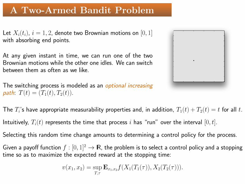
Let Xi(ti), i = 1, 2, denote two Brownian motions on [0, 1]with absorbing end points.

At any given instant in time, we can run one of the twoBrownian motions while the other one idles. We can switchbetween them as often as we like.

The switching process is modeled as an optional increasingpath: T (t) = (T1(t), T2(t)).

The Ti’s have appropriate measurability properties and, in addition, T1(t) + T2(t) = t for all t.

Intuitively, Ti(t) represents the time that process i has “run” over the interval [0, t].

Selecting this random time change amounts to determining a control policy for the process.

Given a payoff function f : [0, 1]2 → IR, the problem is to select a control policy and a stoppingtime so as to maximize the expected reward at the stopping time:

v(x1, x2) = supT,τ

Ex1,x2f (X1(T1(τ )), X2(T2(τ ))).

Optimal Solution

The value function v is the smallest bi-excessive majorant of f :

∂2v

∂x21

≤ 0

∂2v

∂x22

≤ 0

v ≥ f

For simplicity, we henceforth assume that f is zero in the interior of the state space and isgiven by nonnegative concave functions on the four sides of the state space.

With this assumption on f it is easy to see that, given a switching strategy T , the optimalstopping time τ is precisely the first exit time from the interior of the state space.

Larry’s Principle of Smooth Fit

Assume that the concave functions on the “north” and “east” sides are identically zero.

Let γ1(x1) denote the nonnegative concave function along the bottom side.Let γ2(x2) denote the nonnegative concave function along the left side.

Thought experiment...

• Assume that the γi’s are strictly concave.

• Consider being close to the bottom side.

• The value function v will equal γ1 at the boundary.

• If the value function is smooth, then it too will be concave near this lower edge.

• Hence, the optimal strategy is to control vertically. That is, ∂2v/∂x22 = 0.

• A similar analysis applies to the left hand side.

• Posit the existance of a curve coming from the lower left corner representing a switch inpolicy.

• Use the principle of smooth fit to write down differential equation with boundary conditions.

• Solve the differential equation.

The Switching Curve

For any strictly concave function γ, let Γ denote the increasing function given by

Γ(x) = −∫ x

0

uγ ′′(u)du.

The switching curve is given byΓ2(x2) = Γ1(x1).

A similarly explicit formula exists for the value function itself.

When γ1 = γ2, the switching curve is the diagonal.In this case, the switched process involves a local time process on the diagonal.

In general, the behavior of the optimally controlled process has a general local-time-like behavioralong the switching curve.

An Example

0 0.1 0.2 0.3 0.4 0.5 0.6 0.7 0.8 0.9 1−1

−0.8

−0.6

−0.4

−0.2

0

0.2

0.4

0.6

0.8

1

0 0.1 0.2 0.3 0.4 0.5 0.6 0.7 0.8 0.9 10

0.05

0.1

0.15

0.2

0.25

0.3

0.35

0 0.1 0.2 0.3 0.4 0.5 0.6 0.7 0.8 0.9 10

0.1

0.2

0.3

0.4

0.5

0.6

0.7

0.8

0.9

1

0 0.1 0.2 0.3 0.4 0.5 0.6 0.7 0.8 0.9 1−1

−0.8

−0.6

−0.4

−0.2

0

0.2

0.4

0.6

0.8

1

0 0.1 0.2 0.3 0.4 0.5 0.6 0.7 0.8 0.9 10

0.1

0.2

0.3

0.4

0.5

0.6

0.7

0.8

0.9

1

Red zone: run X2. Blue zone: run X1.

A Symmetric Example

0 0.1 0.2 0.3 0.4 0.5 0.6 0.7 0.8 0.9 1−1

−0.8

−0.6

−0.4

−0.2

0

0.2

0.4

0.6

0.8

1

0 0.1 0.2 0.3 0.4 0.5 0.6 0.7 0.8 0.9 10

0.05

0.1

0.15

0.2

0.25

0 0.1 0.2 0.3 0.4 0.5 0.6 0.7 0.8 0.9 10

0.1

0.2

0.3

0.4

0.5

0.6

0.7

0.8

0.9

1

0 0.1 0.2 0.3 0.4 0.5 0.6 0.7 0.8 0.9 1−1

−0.8

−0.6

−0.4

−0.2

0

0.2

0.4

0.6

0.8

1

0 0.1 0.2 0.3 0.4 0.5 0.6 0.7 0.8 0.9 10

0.05

0.1

0.15

0.2

0.25

Red zone: run X2. Blue zone: run X1.

Concave On All Sides

Thinking locally about the corners, one might posit that the general solution looks like this(or its transpose)...

0 0.1 0.2 0.3 0.4 0.5 0.6 0.7 0.8 0.9 10

0.05

0.1

0.15

0.2

0.25

0.3

0.35

0 0.1 0.2 0.3 0.4 0.5 0.6 0.7 0.8 0.9 10

0.02

0.04

0.06

0.08

0.1

0.12

0.14

0.16

0.18

0 0.1 0.2 0.3 0.4 0.5 0.6 0.7 0.8 0.9 10

0.1

0.2

0.3

0.4

0.5

0.6

0.7

0.8

0.9

1

0 0.1 0.2 0.3 0.4 0.5 0.6 0.7 0.8 0.9 10

0.02

0.04

0.06

0.08

0.1

0.12

0.14

0.16

0.18

0 0.1 0.2 0.3 0.4 0.5 0.6 0.7 0.8 0.9 10

0.05

0.1

0.15

0.2

0.25

0.3

0.35

where the switching curves are given by formulae similar to the simple two-sided case.

But Sometimes...

The answer (discovered by solving a linear programming problem), looks like this:

0 0.1 0.2 0.3 0.4 0.5 0.6 0.7 0.8 0.9 10

0.02

0.04

0.06

0.08

0.1

0.12

0.14

0.16

0.18

0 0.1 0.2 0.3 0.4 0.5 0.6 0.7 0.8 0.9 10

0.02

0.04

0.06

0.08

0.1

0.12

0.14

0.16

0.18

0 0.1 0.2 0.3 0.4 0.5 0.6 0.7 0.8 0.9 10

0.1

0.2

0.3

0.4

0.5

0.6

0.7

0.8

0.9

1

0 0.1 0.2 0.3 0.4 0.5 0.6 0.7 0.8 0.9 10

0.02

0.04

0.06

0.08

0.1

0.12

0.14

0.16

0.18

0 0.1 0.2 0.3 0.4 0.5 0.6 0.7 0.8 0.9 10

0.02

0.04

0.06

0.08

0.1

0.12

0.14

0.16

0.18

The central region is an indifference zone—run either Brownian motion.The shape of the indifference zone is always rectangular.

An Example with a Large Indifference Zone

0 0.1 0.2 0.3 0.4 0.5 0.6 0.7 0.8 0.9 10

0.2

0.4

0.6

0.8

1

1.2

1.4

1.6

1.8

2

0 0.1 0.2 0.3 0.4 0.5 0.6 0.7 0.8 0.9 10

0.2

0.4

0.6

0.8

1

1.2

1.4

1.6

0 0.1 0.2 0.3 0.4 0.5 0.6 0.7 0.8 0.9 10

0.1

0.2

0.3

0.4

0.5

0.6

0.7

0.8

0.9

1

0 0.1 0.2 0.3 0.4 0.5 0.6 0.7 0.8 0.9 10

0.2

0.4

0.6

0.8

1

1.2

1.4

0 0.1 0.2 0.3 0.4 0.5 0.6 0.7 0.8 0.9 10

0.2

0.4

0.6

0.8

1

1.2

1.4

The Linear Programming Problem

minimize

∫∫v(x1, x2)dx1dx2

subject to∂2v

∂x21

≤ 0

∂2v

∂x22

≤ 0

v≥ f.

Note: Discretize to make infinite dimensional problem into finite dimensional LP.

PS. Much faster than value iteration!

Optimal Switching References

• Optimal Stopping and Supermartingales over Partially Ordered Sets,Mandelbaum and Vanderbei,Z. Wahrscheinlichkeitstheorie verw. Gebiete, 57, 253–264, 1981

• Optimal Switching Between a Pair of Brownian Motions,Mandelbaum, Shepp, and Vanderbei,Ann. Prob., 18(3), 1010–1033, 1990.

• Optimal Switching Among Several Brownian Motions,Vanderbei,SIAM J. on Control and Optimization, 30, 1150–1162, 1992.

• Brownian Bandits,Mandelbaum and Vanderbei,Dynkin Festschrift, AMS, 1995

Zeros of Random Polynomials

Consider a random polynomial:

Pn(z) =n∑j=0

ηjzj, z ∈ C,

where η0, . . . , ηn are independent standard normal random variables.Let νn(Ω) denote the number of zeros in a set Ω in the complex plane.

Theorem

For each measurable set Ω ⊂ C,

Eνn(Ω) =

∫Ω

hn(x, y)dxdy +

∫Ω∩IR

gn(x)dx,

where

hn =B2D

20 −B0(B

21 + |A1|2) + B1(A0A1 + A0A1)

π|z|2D30

,

and

gn =(B0B2 −B2

1)1/2

π|z|B0

and where

Bk(z) =n∑j=0

jk|z|2j, z ∈ C, k = 0, 1, 2,

Ak(z) =n∑j=0

jkz2j, z ∈ C, k = 0, 1,

and

D0(z) =√B2

0(z)− |A0|2(z).

Main Idea

From the argument principle, we get

νn(Ω) =1

2πi

∫∂Ω

P ′n(z)

Pn(z)dz.

Taking the expectation operator inside the integral, we just need to evaluate the expected valueof the ratio of two (dependent) Gaussian random variables.

The rest is tedious (and perhaps nontrivial) algebra.

Larger n

n = 36

In the paper, we give an explicit formula for the limit as n→∞.

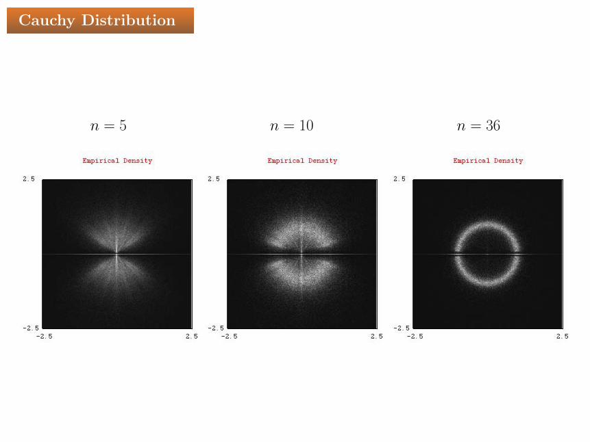
Cauchy Distribution

n = 5 n = 10 n = 36

Zeros of Random Polynomial References

• The Complex Zeros of Random Polynomials,Shepp and VanderbeiTransactions of the AMS, 347(11):4365-4384, 1995

The Dishonest Statistician

This is the era of Big Data: statistics trumps science. Cause-and-effect is passe. Correlationtells all.

Example: Consider a coin to be used in coin tossing.It is important that the coin be fair: p = q = 1/2.

The coin in question appears to the eye to be perfectly symmetric. Physically, it seems fair(and the tosser is a well-respected member of the coin tossing community).

Such appeals to reason are not sufficient. A statistician has been hired to verify the fairness ofthe coin.

The statistician embarks on data collection. He instructs the tosser to toss the coin. Thestatistician keeps track of the number of flips, t, and the difference, Xt, between the numberof heads and tails.

The Dishonest Statistician’s Optimal Stopping Problem

Unfortunately, unbeknownst others, the statistician is dishonest and has a special interest inreporting that the coin is biased in favor of heads.

The only tool at the statistician’s disposal is to stop the experiment at some point when headsoutnumbers tails.

So, the statistician wants to solve an optimal stopping problem:

v(t, x) = supτ≥t

Et,x(Xτ/τ ).

Of course, the statistician wants to know v(0, 0) but he also wants to know the strategy toachieve that “value” and to do that he needs to compute v(t, x) for all t and x.

Hamilton-Jacobi-Bellman Equation

v(t, x) = max

(x

t,v(t + 1, x + 1) + v(t + 1, x− 1)

2

).

Some Old Papers on the Dishonest Statistician

• L. Breiman, “Stopping Rule Problems”, Applied Combinatorial Mathematics, 1964.

– Posed the problem.

• Y.S. Chow and H. Robbins, “On Optimal Stopping Rules for Sn/n”, Z. Wahrscheilichkeit-stheorie und Verw. Gebiete, 1963.

– There exist constants βt such that the optimal stopping rule is to stop the first timethat Xt ≥ βt.

• A. Dvoretzky, “Existence and Properties of Certain Optimal Stopping Rules”, Proc. 5thBerkeley Symp. Math. Statist. Prob., 1967.

– Showed that 0.32 < βt/√t < 4.06.

• L.A. Shepp, “Explicit Solutions to some Problems of Optimal Stopping”, Annals of Math-ematical Statistics, 1969.

– Explicit formula for the limit

α := limt→∞

βt/√t = 0.83992369506 . . .

where

α = (1− α2)

∫ ∞0

eλα−λ2/2dλ

A Few New Papers

• Luis A. Medina, Doron Zeilberger,“An Experimental Mathematics Perspective on the Old, and still Open, Question of WhenTo Stop?”,in Gems in Experimental Mathematics, AMS Contemporary Math., 517, 265–274, 2010

• O. Haggstrom and J. Wastlund,“Rigorous Computer Analysis of the Chow-Robbins Game”,American Mathematical Monthly, 2013.

max

(x

t, 0

)≤ v(t, x) ≤ max

(x

t, 0

)+ min

(1

2

√π

t,

1

|x|

)

Stopping Thresholds

0 2 4 6 8 10 12

x 104

0

50

100

150

200

250

300

350

400

450

tosses

he

ad

exce

ss

β

t low bound

βt up bound

α t1/2

0.792945408 ≤ p = (1 + v(0, 0))/2 ≤ 0.7929841248

Stopping Thresholds – Near the Beginning

0 20 40 60 80 100 1200

1

2

3

4

5

6

7

8

9

tosses

he

ad

exce

ss

β

t low bound

βt up bound

α t1/2

0.792945408 ≤ p = (1 + v(0, 0))/2 ≤ 0.7929841248

Stopping Thresholds – Log-Log Plot

100

101

102

103

104

105

10−1

100

101

102

103

tosses

he

ad

exce

ss

β

t low bound

βt up bound

α t1/2

0.792945408 ≤ p = (1 + v(0, 0))/2 ≤ 0.7929841248

Slightly More Honest Statistician

Even Number of Tosses Only

Only allowed to stop after an even number of tosses.

Modified Bellman equation:

v(t, x) = max

(x

t,v(t + 2, x + 2) + 2v(t + 2, x) + v(t + 2, x− 2)

4

).

Stopping Thresholds – Even Number of Tosses Only

0 2 4 6 8 10 12

x 104

0

50

100

150

200

250

300

350

tosses

he

ad

exce

ss

β

t low bound

βt up bound

α t1/2

0.69730 = p = (1 + v(0, 0))/2 = 0.69733

Stopping Thresholds – Even Number of Tosses Only

0 50 100 150 200 2500

2

4

6

8

10

12

tosses

he

ad

exce

ss

β

t low bound

βt up bound

α t1/2

0.69730 = p = (1 + v(0, 0))/2 = 0.69733

Stopping Thresholds – Even Number of Tosses Only

100

101

102

103

104

105

100

101

102

103

tosses

he

ad

exce

ss

β

t low bound

βt up bound

α t1/2

0.69730 = p = (1 + v(0, 0))/2 = 0.69733

Thank You!