Mon. Not. R. Astron. Soc. 000, 000–000 (2015) Printed 23 September 2018 (MN LATEX style file v2.2)

Frequency dependent core shifts and parameter estimation for theblazar 3C 454.3

P. Mohan1?, A. Agarwal1,2, A. Mangalam3, Alok C. Gupta1,2,4†, Paul J. Wiita5, A. E. Volvach6,7,M. F. Aller8, H. D. Aller8, M. F. Gu4, A. Lahteenmaki9, M. Tornikoski9, L. N. Volvach6,7

1Aryabhatta Research Institute of Observational Sciences (ARIES), Manora Peak, Nainital - 263002, India.2Department of Physics, DDU Gorakhpur University, Gorakhpur - 273009, India.3Indian Institute of Astrophysics, Sarjapur Road, Koramangala, Bangalore - 560034, India.4Key Laboratory for Research in Galaxies and Cosmology, Shanghai Astronomical Observatory, Chinese Academy of Sciences, Shanghai 200030.5Department of Physics, The College of New Jersey, P.O. Box 7718, Ewing, NJ 08628, U.S.A.6Radio Astronomy Laboratory of Crimean Astrophysical Observatory, Crimea.7Taras Shevchenko National University of Kyiv, Kiev, Ukraine.8Astronomy Department, University of Michigan, Ann Arbor, MI, U.S.A.9Aalto University Metsahovi Radio Observatory, Finland.

Accepted 2015 June 22; Received 2015 June 11; in original form 2015 March 12.

ABSTRACT

We study the core shift effect in the parsec scale jet of the blazar 3C 454.3 using the 4.8GHz - 36.8 GHz radio light curves obtained from three decades of continuous monitoring.From a piecewise Gaussian fit to each flare, time lags ∆t between the observation frequenciesν and spectral indices α based on peak amplitudes A are determined. From the fit ∆t ∝ν1/kr , kr = 1.10 ± 0.18 indicating equipartition between the magnetic field energy densityand the particle energy density. From the fit A ∝ να, α is in the range −0.24 to 1.52. Amean magnetic field strength at 1 pc, B1 = 0.5 ± 0.2 G, and at the core, Bcore = 46 ± 16mG, are inferred, consistent with previous estimates. The measure of core position offset isΩrν = 6.4± 2.8 pc GHz1/kr when averaged over all frequency pairs. Based on the statisticaltrend shown by the measured core radius rcore as a function of ν, we infer that the synchrotronopacity model may not be valid for all cases. A Fourier periodogram analysis yields power lawslopes in the range −1.6 to −3.5 describing the power spectral density shape and gives bendtimescales in the range 0.52− 0.66 yr. This result, and both positive and negative α, indicatethat the flares originate from multiple shocks in a small region. Important objectives met inour study include: the demonstration of the computational efficiency and statistical basis ofthe piecewise Gaussian fit; consistency with previously reported results; evidence for the coreshift dependence on observation frequency and its utility in jet diagnostics in the region closeto the resolving limit of very long baseline interferometry observations.

Key words: galaxies: active – (galaxies:) quasars: general – (galaxies:) quasars: individual:3C 454.3 – methods: data analysis

1 INTRODUCTION

Two groups of objects, BL Lacertae (BL Lac; with featureless op-tical spectra) and flat spectrum radio quasar (FSRQ; having promi-nent emission lines) constitute a subset of radio-loud Active Galac-tic Nuclei (RL-AGNs) called blazars, which according to the ori-entation based unified schemes of RL AGNs have jets making an

? E-mail: pmohan@aries.res.in† CAS Visiting Fellow

angle of 6 10 or so to the line of sight (e.g. Urry & Padovani1995). AGNs are characterized by strong flux variability at allwavelengths, strong and variable polarization in the radio to opticalwavelengths, and a core dominated radio spectrum. Blazar emis-sion from the relativistic jet is dominated by non thermal emis-sion (synchrotron and inverse Compton) which is Doppler boostedmaking a cone angle of ∼ 1/Γ where Γ is the bulk Lorentz fac-tor. Flicker in radio flux from these AGN can be caused by inter-stellar scintillation. The apparent extremely high brightness tem-peratures of > 1017K inferred from radio observations can be

c© 2015 RAS

arX

iv:1

506.

0713

7v1

[as

tro-

ph.H

E]

23

Jun

2015

2 Mohan et al.

attributed to relativistic beaming, coherent radiation mechanismsand geometric effects (Wagner & Witzel 1995). Periodic variabil-ity in the blazar might be caused by the helical movement of thejet components, shocks, jet precession effects, accretion disc in-stabilities (Honma et al. 1991; Camenzind & Krockenberger 1992;Gopal-Krishna & Wiita 1992; Gomez et al. 1997; Bach et al. 2006;Britzen et al. 2010) or due to the rotation of the secondary blackhole around the primary supermassive black hole (e.g. Sillanpaaet al. 1988; Valtonen et al. 2008; Rieger & Mannheim 2000).Doppler boosting shortens the variability timescales by a factor ofδ−1 where this Doppler factor depends on the Lorentz factor asδ = 1/Γ(1 − β cos θ) where θ is the angle between the jet direc-tion and the observer line of sight and β = (1 − Γ−2)1/2 is thespeed of the jet component in the source frame.

3C 454.3 (PKS 2251+158) is a highly variable blazar, classi-fied as a FSRQ with redshift z = 0.859 (e.g. Hewitt & Burbidge1989; Jorstad et al. 2001) with a black hole mass of 4.4× 109 M(Gu, Cao & Jiang 2001). An ultra-violet excess due to the domi-nance of thermal emission from the accretion disc over synchrotronradiation is inferred in Raiteri et al. (2007, 2008). Since 2001, theFSRQ has displayed strong variability over the entire electromag-netic spectrum. It underwent a bright outburst almost simultane-ously from radio to X-ray bands in May 2005 when it reached itsbrightest R band magnitude of 12.0 (Fuhrmann et al. 2006; Vercel-lone et al. 2010; Villata et al. 2006, 2007; Raiteri et al. 2008; Jorstadet al. 2010). Flux variations at 230 GHz were detected around twomonths after the optical variations. This outburst was inferred tobe caused by shocks propagating along the relativistic jet whenthe emitting region at optical wavelength passes closest to the ob-server’s line of sight first and does so later on for other wavelengths(Villata et al. 2007). The 2005 outburst was followed by a compar-atively quiescent period till spring 2007 at all frequencies, whenit displayed a “big blue bump”, characteristic of radio-quiet AGNsand indicating thermal emission from the accretion disc (Raiteriet al. 2007). Katarzynski & Ghisellini (2007) proposed a model toexplain the activities of the FSRQ during 2005-2007 time period,according to which the location from which bulk kinetic energyis dissipated along the jet is dependent on the bulk Lorentz factorand compactness of the perturbations which arise. Correlations be-tween light curves at different frequencies during the 2005-2006flare established that a single radiation mechanism is responsiblefor both radio and optical emission. Observations were carried outon all possible timescales, i.e., from days to years, in both opticaland radio from which it was found that the duration of the flare andthe individual features of the flare were same in both, thus showingthat both were produced by the Doppler boosted relativistic jet.

A multiwavelength monitoring campaign during a high fluxstate in 2008 (Bonning et al. 2009) indicates a strong correlationbetween infrared, optical, ultraviolet and γ-ray wavelengths. Thisis attributed to the external Compton scattering where accretiondisk and emission line photons are scattered by strongly relativis-tic electrons (with Lorentz factors 103 − 104) which are also ra-diating synchrotron based infrared and optical emission. A studyof intra-day variability in the source during 2009 - 2010 (Gaur,Gupta & Wiita 2012) during a high flux state indicates a strongcorrelation between the γ-ray and optical wavelengths and that theformer leads the latter by 4.5± 1.0 days and is attributed to exter-nal Compton scattering. A multi frequency study from millimeterwavelengths to γ-rays during three outburst events in 2009 - 2010(Jorstad et al. 2013) reveals a similar radiation mechanism and lo-cation of the flares with small to no time lag being found betweenoptical and γ-ray light curves. Typical variability timescales are in-

ferred to be ∼ 3 hours in the parsec scale jet adding to the conclu-sion that the emission is highly localized. The measured magneticfield strength is in the range 0.1 − 1 G. A study to derive the bulkkinetic power using jet parameters derived in the framework of theKonigl (1981) inhomogeneous jet model at the 43 GHz observa-tional frequency indicates a jet viewing angle of 3.8, bulk Lorentzfactor of 32.4 and Doppler factor of 20.3 (Gu, Cao & Jiang 2009).From the derived bulk kinetic luminosity and the luminosity fromthe broad line emission (due to disk based sources), the study in-fers a strong correlation between these two indicating that the jetpower is intrinsically linked to the accretion process. Owing to itshigh flux state and broadband spectral energy distribution (SED), itoffers opportunities for intra-day variability (IDV) studies (Tavec-chio et al. 2010) as well as spectral variability studies. A study ofthe relationship between the bulk Lorentz factor and the AGN prop-erties (Chai, Cao & Gu 2012) estimates jet parameters derived inthe framework of the inhomogeneous jet model (Konigl 1981). Amagnetic field strength at 1 pc of 0.493 G was obtained, and fromthe large sample of radio-loud AGN, a strong correlation is inferredbetween the bulk Lorentz factor and the black hole mass, indicatingthat accretion and the resulting black hole spin up could play a rolein jet power.

In section 2, we describe parameters that can be derived fromthe analysis of the radio light curves, including the magnetic fieldstrength and size of emitting core, based on physical models pro-posed in earlier literature. In section 3, we describe the observationsmade to obtain the final analyzable light curves and the analysisprocedure which includes a piecewise Gaussian fit to each flaringportion in the light curve. In this section, we then describe the timeseries analysis of each light curve segment using the Fourier peri-odogram. In section 4, the results of the analysis and the estimatedparameters including the time lags, spectral indices, magnetic fieldstrength, size of emitting core and others are presented. This is fol-lowed by a discussion of the results from the time series analysis.We finally conclude in section 5 with the comparison of our resultswith earlier work and its impact.

2 FREQUENCY-DEPENDENT CORE SHIFTS

Due to finite VLBI resolution, the true optically thick radio core(i.e. surface with optical depth τ = 1) is not completely resolved.Since the τ = 1 surface is frequency dependent (Konigl 1981;O’Sullivan & Gabuzda 2009), the radio core position depends onthe observation frequency ν as r ∝ ν−1/kr (Konigl 1981), with rbeing the distance from the central region and the index kr givenby (Lobanov 1998),

kr =(3− 2α)m+ 2n− 2

5− 2α(1)

under the assumption that the ambient medium pressure on thejet is negligible (Konigl 1981; Lobanov 1998) and external pres-sure is non-negligible with non-zero gradient along the jet. In theabove expression for kr , α is the spectral index (S ∝ να) whilem and n describe the power law decay of the magnetic field (B =B1(r/1pc)−m) and particle number density (N = N1(r/1pc)−n)respectively, with distance from the jet base (i.e. the jet apex). HereN1 and B1 refer to values of N and B at a distance of r = 1pc from the core in the observer’s frame. These power law expres-sions are valid till ∼ 1 pc as the jet shape changes from conicalto parabolic closer to the true jet origin (e.g., Krichbaum et al.2006; Asada & Nakamura 2012; Nakamura & Asada 2013; Be-skin & Nokhrina 2006; McKinney 2006). Assuming equipartition

c© 2015 RAS, MNRAS 000, 000–000

Frequency dependent core shifts and parameter estimation for the blazar 3C 454.3 3

between electron energy density and the magnetic energy densitywe obtain n = 2m (Lobanov 1998). Assuming the combinationm = 1 and n = 2 which describes well the synchrotron emissionfrom compact VLBI cores (Konigl 1981; Lobanov 1998) for con-stant jet flow speed along with constant opening angle, we obtainkr = 1, independent of the spectral index α.

In the shock-in-jet model scenario, shocks are produced as aresult of change in physical quantities such as velocity, electrondensity, magnetic field through the jet or pressure at the base ofthe jet. These shocks propagate down the jet and cause core bright-ening, thus resulting in a flaring state of the source which is fol-lowed by the appearance of a jet component in VLBI images (e.g.Marscher & Gear 1985; Gomez et al. 1997). Let Ron be the dis-tance of the onset of a shock which crosses the τ = 1 surface attime Ti for frequency νi thus giving a flare in the light curve. Thecore position shift with frequency gives time lags between differ-ent frequency light curves. For apparent superluminal motion (e.g.Rees 1967; Turler, Courvoisier & Paltani 2000), the time t in theobserver’s frame passed after the onset of the shock wave at thedistance Ron is (Kudryavtseva et al. 2011)

t =(1 + z) sin θ(R(ν)−Ron(ν))

βappc, (2)

where R is the distance along the jet axis, βapp is the apparentsuperluminal velocity of the jet component and θ is the jet viewingangle.

The time lag between light curves at two frequencies is givenby

∆t = t(νa)− t(νb) (3)

=(1 + z) sin θ

βappc[R(νa)−R(νb) +Ron(νa)−Ron(νb)].

Since r ∝ ν−1/kr , ∆t ∝ ν−1/kr . Hence, the determination oftime lags from the light curves at various frequencies can be usedto determine the index kr .

Ωrν is a measure of the core-position offset in pc(GHz)1/kr

given by (Lobanov 1998)

Ωrν = 4.85× 10−9 ∆rmasDL(1 + z)2

(ν

1/kr1 ν

1/kr2

ν1/kr2 − ν1/kr

1

), (4)

where ∆rmas = µ∆t is the core-position offset (in milli-arcseconds) between two frequencies ν1 and ν2 (in GHz) in termsof the proper motion µ and DL is the luminosity distance in pc.The distance of VLBI core from the base of the jet at frequency νis given by (Lobanov 1998)

rcore(ν) =Ωrνsin θ

ν−1/kr . (5)

Using Eqn. (43) from Hirotani (2005) along with the assumptionof equipartition between magnetic field energy density and particleenergy density, the magnetic field strength in Gauss at 1 pc fromthe jet base is given by

B1∼= 0.025

(Ω3rν(1 + z)2

δ2ϕ sin2 θ

)1/4

, (6)

where θ is the jet viewing angle, ϕ is the jet half-opening angle, δis the Doppler factor, z is the cosmological redshift and Ωrν is thecore-position offset defined in Eqn. (4). Using the above equationsand the assumption that m = 1 for an equipartition magnetic field,

Bcore(ν) = B1r−1core. (7)

1970 1980 1990 2000 2010

8

12

16

(segment1)(segment2)

4.8GHz

8

16

24 8.0GHz

10

20

3014.5GHz

0

9

18

27

36 22GHz

0

20

40

Figure 1. Long-term variability light curves of 3C 454.3 in the 4.8 GHz -36.8 GHz frequency range.

3 OBSERVATIONS AND ANALYSIS TECHNIQUE

The long term light curves of 3C 454.3 at 4.8 GHz, 8.0 GHz and14.5 GHz are obtained from the University of Michigan Radio As-tronomical Observatory (UMRAO) (Aller et al. 1999). The UM-RAO data at 4.8 GHz spans the period between 1978 and 2013,while the 8.0 GHz data spans from 1966 to 2013 and the 14.5 GHzdata covers more than 35 years from 1973 to 2013. Radio mon-itoring at 22.2 and 36.8 GHz were carried out with the 22-m ra-dio telescope (RT-22) of the Crimean Astrophysical Observatory(CrAO) (Volvach 2006). We use modulated radiometers in combi-nation with the registration regime “ON-ON” for collecting datafrom the telescope (Nesterov, Volvach & Strepka 2000). Observa-tions at 37.0 GHz were made with the 14 m radio telescope of AaltoUniversity Metsahovi Radio Observatory in Finland. Data obtainedat Metsahovi and RT-22 were combined in a single array to supple-ment each other. A detailed description of the data reduction andanalysis of Metsahovi data is given in Teraesranta et al. (1998).

The light curves of 3C 454.3 from 4.8 GHz to 36.8 GHz aredisplayed in Fig. 1. Long term monitoring is necessary for studyingand analyzing various properties of AGNs such as the dynamicalevolution, the inner sub-parsec structure, radiation mechanisms andlocation of radiating regions.

The light curve is subjected to pre-processing in order to deter-mine the positions of the maxima and minima which represent theboundaries of the flaring portions. A Gaussian filtering with a suit-able parameter is applied to filter high frequency components andhence determine the extrema in the light curve. Then, a Gaussianfunction of the form

y = Ae[−(t−m)2/(2σ2)], (8)

is used to represent the shape of each flare region in the light curve.The fit is carried out from a base line at the minimum amplitude

c© 2015 RAS, MNRAS 000, 000–000

4 Mohan et al.

of the light curve. Initial values A0, m0 and σ0 are taken to be themaxima values, maxima positions and half the differences betweenconsecutive minima (assuming that a flare would be symmetric) re-spectively. As A0, m0 and σ0 are for a smoothed version of theraw light curve, trial values for A, m and σ are generated basedon regions around these initial values. These trial values accountfor possible values in a region around the flare peak amplitude, po-sitions and the differences in the original light curve. A matrix of(Ai,mi, σi) is constructed for all combinations of trial values ofeach peak. Each three parameter combination is fed into eqn. (8)along with the appropriate t spanning each flare. This procedure iscycled through the entire light curve such that all flares are coveredby the Gaussian fit. For each Gaussian section covering a flare

χ2i =

∑i

(xi(ti)− y(Ai,mi, σi))2

Variance(xi(ti)), (9)

is determined for each section between the minima and the bestfit for that section would be that combination (Ai,mi, σi) whichgives the least value of χ2

i . The 1 σ errors are determined for eachparameter based on the table of χ2

i generated as the distance fromthe best fit minimum χ2 value.

The single Gaussian fit procedure is highly advantageous as itprovides a good computational speed (few to tens of seconds de-pending on parameter grid size); the possibility of using a finelysampled grid of trial values for A, m and σ with a typical grid sizeof 40000-50000 combinations; better χ2 fit values as evident fromthe data fits and the residuals; ease of procedure in determinationof best fit parameters and associated errors. The light curves andthe best fit Gaussian summed over each segment along with the fitresiduals are presented in Figs. 2, 3, 4 and 5. The residual givenby [y(Ai,mi, σi) − xi(ti)]/Standard Deviation(xi(ti)) is alsocalculated with the best fit (Ai,mi, σi) for each Gaussian segmentand plotted in the lower panels in the above figures.

The light curves were split into two segments, one from thestart of the observations to 2007.0 and the other from 2007.0 tothe end of the observations. This was done to check for consis-tency of results between the first segment and the second segment,to determine any evolution in the fit parameters and due to the na-ture of the flaring in the light curve i.e. the flares before 2007.0are of lower amplitude compared to the post 2007.0 flares. If theentire light curve is run through the Gaussian fit procedure, it islikely to miss out prominent features in the first segment leading toincorrect results. We then conduct a time series analysis of eachlight curve segment using the Fourier periodogram analysis. Asthe periodogram is only applicable to evenly sampled light curves,we performed a linear interpolation and sampled the light curveat regular intervals of 0.1 days, similar to the procedure followedin, e.g. Gonzalez-Martın & Vaughan (2012); Mohan & Mangalam(2014). This evenly sampled light curve is used to determine thepower spectral density (PSD) shape and any statistically significantquasi-periodic oscillations (QPOs). The normalized periodogram isgiven by (e.g. Vaughan et al. 2003),

P (fj) =2∆t

x2N|F (fj)|2 (10)

where ∆t = 0.1 days is the sampling time step, x is the mean ofthe light curve x(tk) of length N points, and |F (fj)| is its discreteFourier transform evaluated at frequencies fj = j/(N∆t) withj = 1, 2, .., (N/2−1). We fit the periodogram with two competingmodels, a power law and a bending power law, in order to describethe PSD shape. The power law model is given by

I(fj) = Afsj + C, (11)

with amplitude A, slope s, and a constant Poisson noise C. Thismodel fits optical/ultra-violet and X-ray data reasonably well asinferred from previous studies (e.g. Gonzalez-Martın & Vaughan2012; Mohan & Mangalam 2014) and could thus represent broad-band variability across a wide range of Fourier frequencies in mul-tiple wavelengths. The bending power law model is given by

I(fj) = Af−1j

(1 + (fj/fb)

−s−1)−1+ C. (12)

with amplitude A, slope s, bend frequency fb, and a constantPoisson noise C. The model is a special case of the generalizedbending knee model (McHardy et al. 2004). The maximum likeli-hood estimator (MLE) method is used to determine model param-eters in which the log-likelihood function (e.g. Emmanoulopoulos,McHardy & Papadakis 2013; Mohan, Mangalam & Chattopadhyay2014; Mohan & Mangalam 2014) defined by

S(θk) = −2

n−1∑j=1

(ln(I(fj , θk)) + P (fj)/I(fj , θk)), (13)

is first determined. Here, I(fj , θk) are the power law or bend-ing power model with parameters θk. Determining θk which mini-mize S yields the maximum likelihood values. The log-likelihoodS is determined for a large number of combinations of the pa-rameters θk for a given model. The parameter combination whichgives a unique global minimum Smin yields the best fit. For Si cor-responding to each unique combination of the parameters θk, as∆S = Si−Smin are approximately χ2

k distributed, the cumulativedistribution function of the χ2

k distribution is used to estimate pa-rameter confidence intervals. The ∆S determined from the param-eter combinations within a desired confidence interval are grouped.Parameter ranges that they correspond to are used to determine con-fidence intervals of the θk used in a given model.

For model selection, we use the Akaike information criteria(AIC) (e.g. Burnham & Anderson 2004) which measures the infor-mation lost when a model is fit to the data. The model with leastinformation loss (least AIC) is the best fit. A likelihood function Lwhich is proportional to the probability of the success of the modelin describing the PSD shape is evaluated for each model. The AICand likelihood are defined by

AIC = S(θk) + 2pk, (14)

∆i = AICmin(model i) −AICmin(null),

L(model i|data) = e−∆i/2,

where pk, the penalty term, is the number of parameters θk used inthe model, and L(model i|data) is the likelihood of model i giventhe data. Models with ∆i 6 2 can be considered close to the bestfit, those with 4 6 ∆i 6 7 are considerably less supported, andthose with ∆i > 10 cannot be supported (Burnham & Anderson2004). As the residual γ(fj) = P (fj)/I(fj) follows the χ2

2 distri-bution, the area under the tail of the probability density function ofthe χ2

2 distribution (gamma density Γ(1, 1/2) = exp (−x/2)/2)gives the probability ε that the power deviates from the mean ata given frequency and is measured in units of standard deviationgiven by γε. We must correct γε to account for the K number oftrial frequencies at which the periodogram is evaluated and so isgiven by (Vaughan 2005),

γε = −2 ln[1− (1− ε)1K ]. (15)

Once ε (e.g. 0.95, 0.99) is specified, γε is calculated and multipliedwith I(fj) to give the significance level used to identify outliers inthe periodogram that could indicate the presence of a QPO.

c© 2015 RAS, MNRAS 000, 000–000

Frequency dependent core shifts and parameter estimation for the blazar 3C 454.3 5

8

10

12

14

16

18

10

15

20

Figure 2. Segment 1 (beginning of observations to ∼ 2007.0) of the4.8 GHz, 8.0 GHz and 14.5 GHz light curve flares fit with a piecewiseGaussian function. The residual in the lower panels are calculated as[y(Ai,mi, σi)− xi(ti)]/Standard Deviation(xi(ti)).

Figure 3. Segment 1 (beginning of observations to ∼ 2007.0) of the 22.0GHz and 36.8 GHz light curve flares fit with a piecewise Gaussian func-tion. The residual in the lower panels are calculated as [y(Ai,mi, σi) −xi(ti)]/Standard Deviation(xi(ti)).

4 RESULTS AND DISCUSSION

For a flare X observed in multiple frequencies ν, mX,ν1 −mX,ν2 = ∆tX where ∆tX is the time lag between the flare inν1 and ν2 with ν1 > ν2. The parameters derived from the Gaus-sian fit procedure discussed in section 3 are presented in Table 1for the first segment and in Table 2 for the second segment. In bothtables, column 1 presents the flare nomenclature; column 2 givesthe observed frequency, column 3 gives the maximum amplitudeof the flare at a particular frequency; column 4 gives the epoch ofthe maximum flare amplitude; column 5 gives the full width at halfmaxima obtained from Gaussian fit for the particular flare; column6 gives the calculated time lags and column 7 gives the spectralindex for each flare.

We fit time lags (∆tX ) derived from the Gaussian fits de-scribed in section 3 with a function ∆t = aν−1/kr + b using aweighted non-linear least squares method. The median of each pa-rameter and the associated median deviation are reported below.Those portions that were not fit well due to either too small a num-ber of points or unstable numerical results are excluded in the cal-culation of the parameters. The results of ∆t versus ν are plotted

c© 2015 RAS, MNRAS 000, 000–000

6 Mohan et al.

10

15

20

Figure 4. Segment 2 (2007.0 to end of observations) of the 4.8 GHz, 8.0GHz and 14.5 GHz light curve flares fit with a piecewise Gaussian func-tion. The residual in the lower panels are calculated as [y(Ai,mi, σi) −xi(ti)]/Standard Deviation(xi(ti)).

Figure 5. Segment 2 (2007.0 to end of observations) of the 22.0 GHzand 36.8 GHz light curve flares fit with a piecewise Gaussian func-tion. The residual in the lower panels are calculated as [y(Ai,mi, σi) −xi(ti)]/Standard Deviation(xi(ti)).

in Fig. 6 for segment 1 and Fig. 7 for segment 2 and the values ofthe fit parameters are:

(i) First segment: beginning of observation – 2007.0

b = −0.28± 0.19 yr

a = 5.51± 1.03 yr (GHz)−1/kr

kr = 0.97± 0.24;

(ii) Second segment: 2007.0 – end of observation

b = −0.06± 0.02 yr

a = 3.03± 0.87 yr (GHz)−1/kr

kr = 1.22± 0.33.

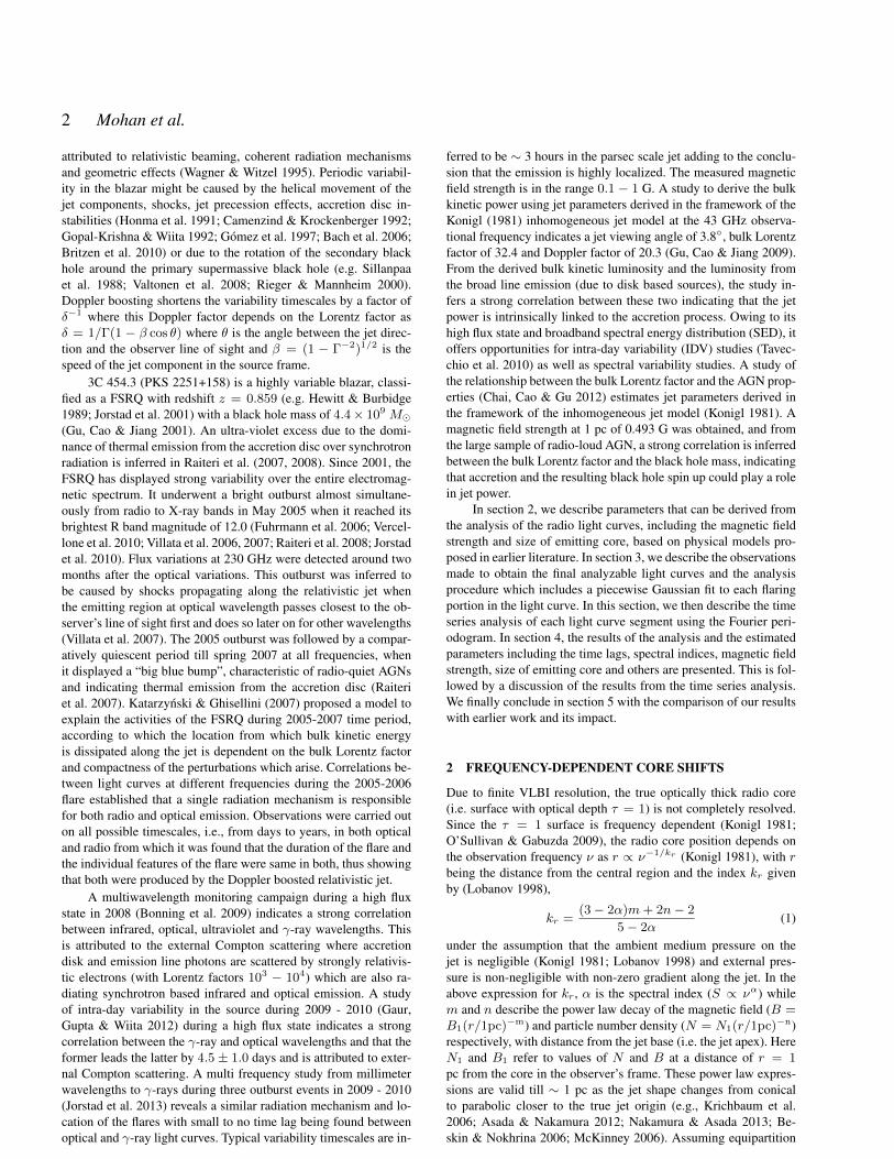
In both light curve segments, the inferred kr are similar andconsistent with equipartition between particle energy density andmagnetic field energy density. From the above fits, we have infor-mation on the amplitude and hence the peak flux for each flare at theobserved frequencies. As S ∝ να, the amplitude versus frequencydata is fit with a functionA = N να to determine the spectral indexα for each flare. The fit is carried out only for flares with four data

c© 2015 RAS, MNRAS 000, 000–000

Frequency dependent core shifts and parameter estimation for the blazar 3C 454.3 7

0 10 20 30

0

0.5

1

1.5

A: 1981.58

B: 1984.74

0 10 20 30

0

0.5

1

1.5C: 1987.21

D: 1989.05

0 10 20 30

0

0.5

1

1.5

E: 1991.00

F: 1993.26

0 10 20 30

0

0.5

1

1.5

G: 1994.05

H: 1995.26

0 10 20 30

0

0.5

1

1.5

I: 1998.69

J: 2000.04

K: 2001.36

I: 1998.69

M: 2006.06

Figure 6. Time lags ∆t as a function of ν for segment 1 light curves. A fitto ∆t = aν−1/kr + b yields b = −0.28± 0.19 yr, a = 5.51± 1.03 yr(GHz)−1/kr and kr = 0.97 ± 0.24. The kr value indicates consistencyof the equipartition between magnetic field energy density and the particlekinetic energy.

0 10 20 30

0

0.2

0.4

0.6

0.8

N: 2006.86

O: 2007.66

0 10 20 30

0

0.2

0.4

0.6

0.8

P: 2007.96

Q: 2008.68

0 10 20 30

0

0.2

0.4

0.6

0.8

R: 2010.31

S: 2010.96

0 10 20 30

0

0.2

0.4

0.6

0.8

T: 2013.78

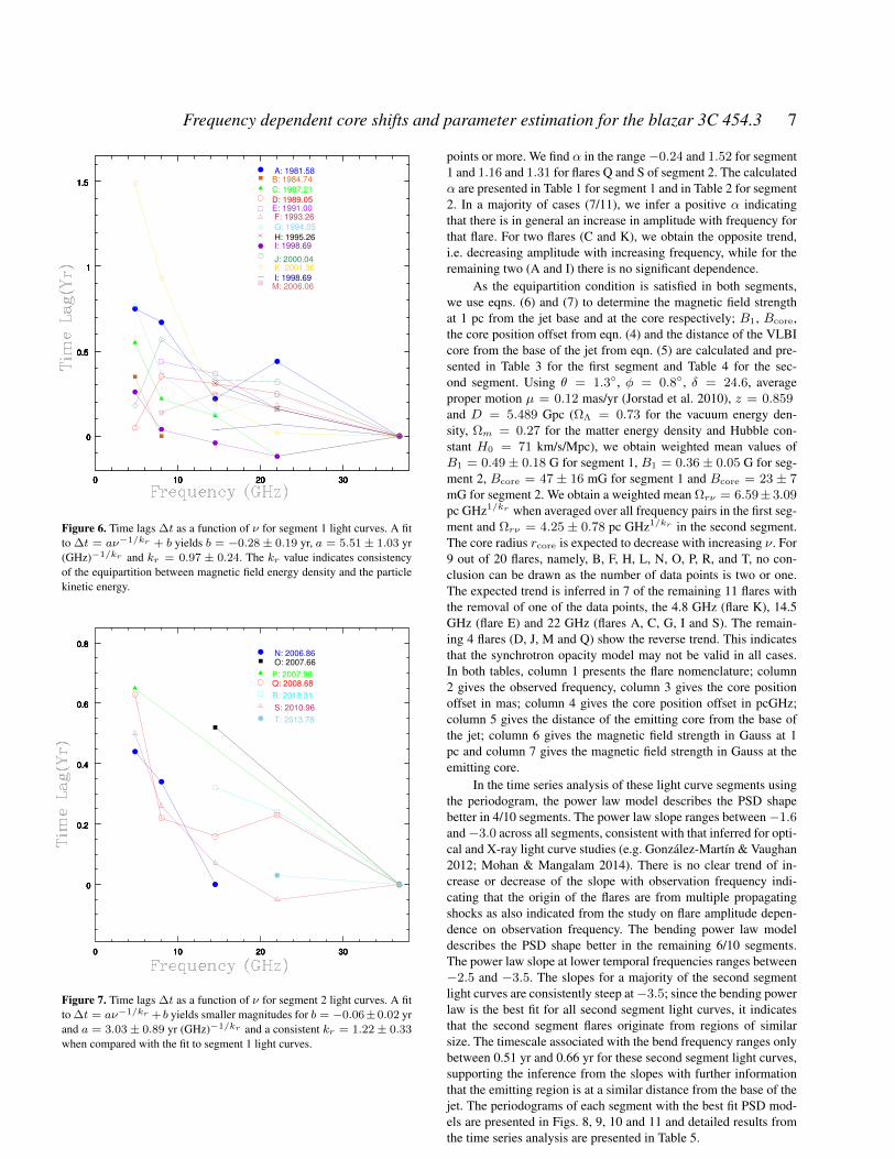
Figure 7. Time lags ∆t as a function of ν for segment 2 light curves. A fitto ∆t = aν−1/kr + b yields smaller magnitudes for b = −0.06±0.02 yrand a = 3.03± 0.89 yr (GHz)−1/kr and a consistent kr = 1.22± 0.33when compared with the fit to segment 1 light curves.

points or more. We find α in the range−0.24 and 1.52 for segment1 and 1.16 and 1.31 for flares Q and S of segment 2. The calculatedα are presented in Table 1 for segment 1 and in Table 2 for segment2. In a majority of cases (7/11), we infer a positive α indicatingthat there is in general an increase in amplitude with frequency forthat flare. For two flares (C and K), we obtain the opposite trend,i.e. decreasing amplitude with increasing frequency, while for theremaining two (A and I) there is no significant dependence.

As the equipartition condition is satisfied in both segments,we use eqns. (6) and (7) to determine the magnetic field strengthat 1 pc from the jet base and at the core respectively; B1, Bcore,the core position offset from eqn. (4) and the distance of the VLBIcore from the base of the jet from eqn. (5) are calculated and pre-sented in Table 3 for the first segment and Table 4 for the sec-ond segment. Using θ = 1.3, φ = 0.8, δ = 24.6, averageproper motion µ = 0.12 mas/yr (Jorstad et al. 2010), z = 0.859and D = 5.489 Gpc (ΩΛ = 0.73 for the vacuum energy den-sity, Ωm = 0.27 for the matter energy density and Hubble con-stant H0 = 71 km/s/Mpc), we obtain weighted mean values ofB1 = 0.49± 0.18 G for segment 1, B1 = 0.36± 0.05 G for seg-ment 2, Bcore = 47 ± 16 mG for segment 1 and Bcore = 23 ± 7mG for segment 2. We obtain a weighted mean Ωrν = 6.59±3.09pc GHz1/kr when averaged over all frequency pairs in the first seg-ment and Ωrν = 4.25 ± 0.78 pc GHz1/kr in the second segment.The core radius rcore is expected to decrease with increasing ν. For9 out of 20 flares, namely, B, F, H, L, N, O, P, R, and T, no con-clusion can be drawn as the number of data points is two or one.The expected trend is inferred in 7 of the remaining 11 flares withthe removal of one of the data points, the 4.8 GHz (flare K), 14.5GHz (flare E) and 22 GHz (flares A, C, G, I and S). The remain-ing 4 flares (D, J, M and Q) show the reverse trend. This indicatesthat the synchrotron opacity model may not be valid in all cases.In both tables, column 1 presents the flare nomenclature; column2 gives the observed frequency, column 3 gives the core positionoffset in mas; column 4 gives the core position offset in pcGHz;column 5 gives the distance of the emitting core from the base ofthe jet; column 6 gives the magnetic field strength in Gauss at 1pc and column 7 gives the magnetic field strength in Gauss at theemitting core.

In the time series analysis of these light curve segments usingthe periodogram, the power law model describes the PSD shapebetter in 4/10 segments. The power law slope ranges between−1.6and−3.0 across all segments, consistent with that inferred for opti-cal and X-ray light curve studies (e.g. Gonzalez-Martın & Vaughan2012; Mohan & Mangalam 2014). There is no clear trend of in-crease or decrease of the slope with observation frequency indi-cating that the origin of the flares are from multiple propagatingshocks as also indicated from the study on flare amplitude depen-dence on observation frequency. The bending power law modeldescribes the PSD shape better in the remaining 6/10 segments.The power law slope at lower temporal frequencies ranges between−2.5 and −3.5. The slopes for a majority of the second segmentlight curves are consistently steep at−3.5; since the bending powerlaw is the best fit for all second segment light curves, it indicatesthat the second segment flares originate from regions of similarsize. The timescale associated with the bend frequency ranges onlybetween 0.51 yr and 0.66 yr for these second segment light curves,supporting the inference from the slopes with further informationthat the emitting region is at a similar distance from the base of thejet. The periodograms of each segment with the best fit PSD mod-els are presented in Figs. 8, 9, 10 and 11 and detailed results fromthe time series analysis are presented in Table 5.

c© 2015 RAS, MNRAS 000, 000–000

8 Mohan et al.

3C 454.3 4.8 GHz : Segment 1

10-6

10-5

10-4

10-3

10-2

10-1

100

101

102

Pow

erde

nsity

(yr-

1 )

(a)

10-1 100

Frequency (yr-1)

10-610-510-410-310-210-1100101

I j/P

j

(b)

3C 454.3 8.0 GHz : Segment 1

10-7

10-6

10-5

10-4

10-3

10-2

10-1

100

101

Pow

erde

nsity

(yr-

1 )

(a)

10-1 100

Frequency (yr-1)

10-310-210-1100101

I j/P

j

(b)

3C 454.3 14.5 GHz : Segment 1

10-6

10-5

10-4

10-3

10-2

10-1

100

101

Pow

erde

nsity

(yr-

1 )

(a)

10-1 100

Frequency (yr-1)

10-310-210-1100101

I j/P

j

(b)

Figure 8. Periodogram analysis of segment 1 (beginning of observations to∼ 2007.0) of the 4.8 GHz, 8.0 GHz and 14.5 GHz light curve flares. Thebest fit model is the solid curve, the dashed curve above it is the 99 % sig-nificance contour which can identify statistically significant quasi-periodiccomponents, the dot-dashed horizontal line is the white noise level and theplot below each periodogram panel shows the fit residuals.

Flare Frequency Amplitude Position Width Time lag Spectral index(GHz) A (Jy) m (year) σ (years) ∆t (years) α

A 36.8 9.28± 0.40 1981.58±0.08 0.86±0.19 0.00 −0.09±0.1322.0 10.97±0.18 1982.02±0.14 0.82±0.39 0.44±0.1614.5 12.63±0.06 1981.80±0.10 0.96±0.51 0.22±0.178.0 12.38±0.30 1982.25±0.09 0.96±0.36 0.67±0.134.8 9.01±0.54 1982.33±0.17 1.02±0.15 0.75±0.19

B 8.0 2.90±0.46 1984.74±0.14 0.39±0.06 0.004.8 3.39±0.10 1985.09±0.16 0.55±0.11 0.35±0.21

C 36.8 4.66±0.36 1987.21±0.02 0.95±0.33 0.00 -0.19 ± 0.1322.0 5.46±0.28 1987.09±0.13 1.54±0.43 -0.12±0.1314.5 7.16±0.02 1987.33±0.06 1.03±0.50 0.12±0.148.0 7.62±0.42 1987.43±0.03 1.17±0.25 0.22±0.074.8 6.98±0.46 1987.76±0.06 1.33±0.27 0.55±0.07

D 36.8 7.22±0.28 1989.05±0.02 0.45±0.27 0.00 0.12 ± 0.0222.0 6.00±0.38 1989.30±0.18 0.48±0.04 0.25±0.1814.5 6.37±0.42 1989.36±0.13 0.55±0.16 0.31±0.228.0 6.21±0.52 1989.40±0.03 0.59±0.18 0.35±0.134.8 5.47±0.14 1989.10±0.01 1.09±0.30 0.05±0.03

E 36.8 6.26±0.56 1991.01±0.09 0.23±0.12 0.00 1.52 ± 0.2322.0 2.45±0.24 1991.16±0.14 0.31±0.08 0.16±0.1714.5 1.67±0.32 1991.37±0.15 0.48±0.10 0.37±0.218.0 0.86±0.28 1991.44±0.03 0.13±0.03 0.44±0.15

F 36.0 8.81±0.08 1993.26±0.05 0.36±0.15 0.0022.0 9.2±0.02 1993.44±0.13 0.98±0.31 0.18±0.14

G 36.8 12.41±0.01 1994.05±0.15 0.41±0.14 0.00 0.16 ± 0.0122.0 12.28±0.30 1994.29±0.08 0.63±0.17 0.24±0.1714.5 15.61±0.24 1994.18±0.02 0.92±0.25 0.13±0.088.0 13.37±0.30 1994.42±0.16 0.77±0.27 0.37±0.164.8 8.94±0.01 1994.82±0.11 1.06±0.37 0.77±0.19

H 36.8 7.50±0.10 1995.26±0.18 0.50±0.01 0.0022.0 8.01±0.42 1995.42±0.07 0.42±0.07 0.16±0.1914.5 7.87±0.20 1995.57±0.19 0.37±0.05 0.31±0.20

I 36.8 4.43±0.34 1998.69±0.10 0.48±0.17 0.00 -0.04 ± 0.0922.0 6.10±0.46 1998.57±0.09 0.36±0.09 -0.12±0.1314.5 6.14±0.26 1998.65±0.16 0.41±0.06 -0.04±0.188.0 5.60±0.14 1998.73±0.17 1.29±0.34 0.04±0.234.8 4.79±0.52 1998.95±0.06 1.22±0.38 0.26±0.18

J 36.8 4.95±0.12 2000.04±0.14 0.77±0.15 0.00 0.08 ± 0.0622.0 5.10±0.08 2000.36±0.05 0.31±0.13 0.32±0.1514.5 4.60±0.12 2000.37±0.13 0.91±0.27 0.33±0.148.0 3.61±0.58 2000.61±0.06 0.28±0.10 0.57±0.144.8 4.41±0.38 2001.22±0.09 0.78±0.26 0.18±0.11

K 36.8 4.37±0.50 2001.36±0.12 1.01±0.18 0.00 -0.24 ± 0.1722.0 4.61±0.04 2001.38±0.14 0.65±0.11 0.02±0.1814.5 5.52±0.10 2001.56±0.03 0.49±0.16 0.20±0.148.0 4.20±0.36 2002.29±0.20 1.46±0.37 0.93±0.204.8 4.21±0.58 2002.85±0.01 1.23±0.31 1.49±0.20

L 36.8 5.27±0.10 2003.20±0.09 0.35±0.08 0.0022.0 4.38±0.20 2003.27±0.12 0.64±0.16 0.07±0.1514.5 5.05±0.36 2003.24±0.01 0.77±0.17 0.04±0.12

M 36.8 17.55±0.02 2006.06±0.03 0.26±0.37 0.00 1.05 ±0.0622.0 8.07±0.44 2006.24±0.18 0.34±0.03 0.16±0.1814.5 5.08±0.50 2006.35±0.05 1.09±0.15 0.25±0.198.0 4.38±0.22 2006.20±0.01 0.58±0.45 0.14±0.05

Table 1. Gaussian fit based parameters, time lags and spectral index forsegment 1 light curves.

5 CONCLUSIONS

The core shift effect in the parsec scale jet of the blazar 3C 454.3was studied in the 4.8 GHz - 36.8 GHz radio wavelengths. Theinferred time delays ∆t for flares in these frequencies are in agree-ment with the frequency dependence of synchrotron emission fromthe core (surface with optical depth τ = 1) (Konigl 1981). Fromthe fit ∆t ∝ ν−1/kr where ν are the observation frequencies, weobtain a weighted mean kr = 1.10 ± 0.18, consistent with theequipartition between the magnetic field energy density and theparticle energy density. The large scale magnetic field thus domi-nates the kinematics of parsec scale jets as its decay is slower com-pared to the decay in the particle number density as Bcore ∝ r−1

and N ∝ r−2. From the fit to the flare amplitudes A ∝ να,we infer spectral indices α in the range −0.24 and 1.52 for both

c© 2015 RAS, MNRAS 000, 000–000

Frequency dependent core shifts and parameter estimation for the blazar 3C 454.3 9

Flare Frequency Amplitude Position Width Time lag Spectral index(GHz) A (Jy) m (year) σ (years) ∆t (years) α

N 14.5 1.08±0.12 2006.85±0.08 0.28±0.12 0.008.0 2.25±0.54 2007.19±0.01 0.23±0.06 0.34±0.084.8 2.15±0.56 2007.29±0.13 0.50±0.15 0.44±0.13

O 36.0 11.19± 0.22 2007.66±0.01 0.15±0.05 0.0022.0 9.50±0.28 2008.06±0.12 0.23±0.02 0.40±0.1214.5 3.25±0.36 2008.18±0.14 0.41±0.20 0.52±0.14

P 36.0 11.61± 0.46 2007.96±0.06 0.17±0.03 0.004.8 1.98±0.24 2008.61±0.23 0.48±0.04 0.65±0.24

Q 36.0 24.44± 0.60 2008.68±0.07 0.26±0.09 0.00 1.16 ± 0.0622.0 15.36±0.06 2008.92±0.04 0.27±0.26 0.24±0.0814.5 9.31±0.18 2008.84±0.04 0.33±0.14 0.16±0.048.0 4.38±0.08 2008.90±0.16 0.60±0.21 0.22±0.164.8 3.57±0.54 2009.31±0.09 1.02±0.15 0.53±0.10

R 36.0 32.43± 0.24 2010.31±0.02 0.34±0.09 0.0022.0 31.85±0.34 2010.54±0.01 0.36±0.12 0.23±0.0214.5 22.34±0.06 2010.63±0.07 0.34±0.15 0.32±0.07

S 36.0 47.99± 0.12 2010.96±0.01 0.28±0.27 0.00 1.31 ± 0.2422.0 35.79±0.16 2010.91±0.01 0.13±0.06 -0.05±0.0114.5 12.63±0.06 2011.03±0.02 0.96±0.51 0.07±0.028.0 14.27±0.24 2011.22±0.32 0.75±0.03 0.26±0.324.8 7.80±0.28 2011.46±0.15 0.85±0.27 0.50±0.35

T 36.0 9.64± 0.04 2013.78±0.01 0.50±0.49 0.0022.0 3.39±0.01 2013.81±0.12 0.30±0.92 -0.03±0.12

Table 2. Gaussian fit based parameters, time lags and spectral index forsegment 2 light curves.

segments. As the shock propagates downstream, it loses energythrough interactions with the plasma. Thus, the amplitude of flaresat lower frequencies is expected to be reduced. The opposite trend,i.e., decreasing amplitude with increasing frequency, can occur ifthe core is excited by shocks that have sufficient energy to causeflaring at lower frequencies but are not energetic enough to causeexcitation upstream at higher frequencies. In our study, we obtainboth positive and negative α. The flaring activity can thus be at-tributed to multiple propagating shocks.

We infer a weighted mean B1 = 0.5 ± 0.2 G and Bcore =46±16 mG considering both segments. These results are consistentwithin error bars of B1 = 0.493 G obtained in Chai, Cao & Gu(2012) andBcore = 0.04±0.02 G obtained in Kutkin et al. (2014).We obtain a weighted mean Ωrν = 6.4 ± 2.8 pc GHz1/kr whenaveraged over all frequency pairs in both segments. The source wasalso studied by Pushkarev et al. (2012) where estimates of Ωrν ,B1

and Bcore for the 15/8 GHz frequency pair are 22 pcGHz (kr = 1was assumed), 1.13 G and 0.06 G respectively. The inferredB1 andBcore range in our study are consistent with these earlier estimates.The shift µ = 0.70 mas/yr was assumed in Kutkin et al. (2014)and as a result, Ωrν = 43 ± 10 pc GHz was obtained. As it wasnoted that the chosen value is 2− 8 times higher than that obtainedin previous studies, we used a lower limit of µ = 0.12 mas/yr ofa range 0.12 - 0.53 mas/yr (Jorstad et al. 2005) at 43 GHz, and0.3 mas/yr at 15 GHz (Lister et al. 2013) to estimate Ωrν whichis the reason for our estimate being ∼ 4 − 15 times smaller thanthat obtained previously. Based on the statistical trend shown bythe rcore as a function of ν, we infer that the synchrotron opacitymodel may not be valid for all cases.

From the time series analysis we obtain typical power lawslopes in the range−1.6 to−3.5 for the power law as well as bend-ing power law PSD shapes at lower temporal frequencies. The anal-ysis indicates that the first segment light curves are consistent withmultiple shock excitation events. The bending power law model isinferred to be a better PSD fit with a−3.5 slope and consistent bendtimescales ranging between 0.51 yr and 0.66 yr for the second seg-

Flare Frequency ∆r Ωrν rcore B1pc Bcore(GHz) (µas) (pc GHz1/kr ) (pc) (G) (mG)

A 4.8 90±16 3.97±0.74 34.84±0.83 0.37±0.05 11±28.0 80±20 6.63±1.67 34.47±1.82 0.55±0.10 16±414.5 26±19 5.16±3.72 14.54±4.02 0.45±0.25 31±2322.0 53±10 23.76±4.52 43.62±4.90 1.43±0.20 33±6

B 4.8 42±17 1.85±0.76 16.26±0.83 0.21±0.06 13±5

C 4.8 66±8 2.91±0.39 25.55±0.45 0.30±0.03 12±28.0 26±17 2.18±1.41 11.32±1.52 0.24±0.12 21±1414.5 14±16 2.81±3.13 7.93±3.38 0.29±0.24 36±4122.0 14±2 6.48±0.91 11.90±0.98 0.54±0.06 45±6

D 4.8 6±16 0.26±0.71 2.32±0.76 0.05±0.10 21±568.0 42±26 3.47±2.15 18.00±2.33 0.34±0.16 19±1214.5 37±22 7.27±4.30 20.49±4.66 0.59±0.26 29±1722.0 30±2 13.50±0.93 24.79±1.02 0.94±0.05 38±3

E 8.0 53±25 4.36±2.07 22.63±2.24 0.40±0.14 18±914.5 44±20 8.68±3.91 24.46±4.24 0.67±0.23 27±1322.0 19±11 8.64±4.95 15.86±5.36 0.67±0.28 42±25

F 22.0 22±6 9.72±2.71 17.85±2.93 0.73±0.02 41± 12

G 4.8 92±19 4.07±0.87 35.77±0.97 0.38±0.06 11±28.0 44±10 3.67±0.84 19.03±0.91 0.35±0.06 19±414.5 16±20 3.05±3.91 8.59±4.23 0.31±0.29 36±4722.0 29±18 12.96±8.10 23.80±8.77 0.91±0.43 38±25

H 14.5 37±23 7.27±4.50 20.49±4.87 0.59±0.27 29±1822.0 19±22 8.64±9.90 15.86±10.71 0.67±0.57 42±53

I 4.8 31±28 1.38±1.24 12.08±1.34 0.17±0.11 14±138.0 5±22 0.40±1.82 2.06±1.96 0.07±0.23 32±15014.5 5±16 0.94±3.13 2.64±3.38 0.13±0.32 48±16022.0 14±12 6.48±5.40 11.90±5.84 0.54±0.34 45±38

J 4.8 22±17 0.95±0.75 8.36±0.81 0.13±0.08 15±128.0 68±17 5.64±1.42 29.32±1.55 0.49±0.09 17±414.5 40±18 7.74±3.52 21.81±3.81 0.62±0.21 28±1322.0 38±17 17.28±7.66 31.73±8.28 1.13±0.37 36±16

K 4.8 179±24 7.88±1.15 69.21±1.32 0.62±0.07 9±18.0 112±17 9.21±1.44 47.84±1.59 0.70±0.08 15±214.5 24±22 4.69±4.30 13.22±4.65 0.42±0.29 32±3022.0 2±14 1.08±6.30 1.98±6.81 0.14±0.62 71±456

L 14.5 5±18 0.94±3.51 2.64±3.81 0.13±0.36 48±18622.0 8±11 3.78±4.95 6.94±5.36 0.36±0.35 52±70

M 8.0 17±23 1.39±1.90 7.20±2.05 0.17±0.17 24±3314.5 30±22 5.86±4.30 16.52±4.65 0.50±0.28 30±2222.0 19±4 8.64±1.81 15.86±1.96 0.67±0.10 42±9

Table 3. Core position offsets, distance from jet base and magnetic fieldstrengths inferred for segment 1 light curves.

Flare Frequency ∆r Ωrν rcore B1pc Bcore(GHz) (mas) (pc GHz1/kr ) (pc) (G) (G)

N 4.8 53±10 1.80±0.36 22.11±0.87 0.21±0.03 9±28.0 41±10 2.40±0.60 19.44±1.40 0.26±0.05 13±3

O 14.5 62±6 8.01±0.80 39.77±1.90 0.63±0.05 16±222.0 11±1 3.03±0.29 10.69±0.67 0.31±0.02 29±3

P 4.8 78±7 2.67±0.30 32.66±0.78 0.28±0.02 8±1

Q 4.8 76±19 2.59±0.67 31.66±1.60 0.27±0.05 9±28.0 26±5 1.56±0.30 12.58±0.71 0.19±0.03 15±314.5 19±10 2.47±1.29 12.24±2.98 0.26±0.10 21±1122.0 28±8 7.73±2.25 27.31±5.22 0.62±0.13 23±7

R 14.5 38±2 4.93±0.29 24.47±0.71 0.44±0.02 18±122.0 29±2 8.07±0.59 28.50±1.38 0.64±0.03 22±2

S 4.8 60±38 2.05±1.31 25.13±3.04 0.23±0.11 9±68.0 31±2 1.84±0.14 14.86±0.36 0.21±0.01 14±114.5 8±1 1.08±0.13 5.35±0.31 0.14±0.01 26±322.0 6±1 1.68±0.28 5.94±0.66 0.20±0.02 33±6

T 22.0 4±1 1.01±0.28 3.56±0.65 0.13±0.03 38±10

Table 4. Core position offsets, distance from jet base and magnetic fieldstrengths inferred for segment 1 light curves.

c© 2015 RAS, MNRAS 000, 000–000

10 Mohan et al.

3C 454.3 22.0 GHz : Segment 1

10-6

10-5

10-4

10-3

10-2

10-1

100

101

102

Pow

erde

nsity

(yr-

1 )

(a)

10-1 100

Frequency (yr-1)

10-310-210-1100101

I j/P

j

(b)

3C 454.3 36.8 GHz : Segment 1

10-5

10-4

10-3

10-2

10-1

100

101

102

Pow

erde

nsity

(yr-

1 )

(a)

10-1 100

Frequency (yr-1)

10-2

10-1

100

101

I j/P

j

(b)

Figure 9. Periodogram analysis of segment 1 (beginning of observations to∼ 2007.0) of the 22.0 GHz and 36.8 GHz light curve flares. The best fitmodel is the solid curve, the dashed curve above it is the 99 % significancecontour which can identify statistically significant quasi-periodic compo-nents, the dot-dashed horizontal line is the white noise level and the plotbelow each periodogram panel shows the fit residuals.

ment light curves indicating that the emitting cores for these flaresare similar in size and distance from the jet base.

Important objectives met in this study include the demonstra-tion of the computational efficiency and statistical basis of the anal-ysis technique involving the piecewise Gaussian fit, which is auto-mated in the determination of relevant flares; the ability to use thisanalysis across a wide range of light curves; the check for and con-firmation of consistency of the results obtained for both light curvesegments; the check for consistency with previously reported re-sults based on a single flare in Kutkin et al. (2014) and the evidenceit provides for the core shift dependence on the frequency and itsusefullness in the determination of a variety of jet diagnostics in theregion close to the resolving limit of VLBI (in the near vicinity ofthe central supermassive black hole).

3C 454.3 4.8 GHz : Segment 2

10-4

10-3

10-2

10-1

100

Pow

erde

nsity

(yr-

1 )

(a)

100

Frequency (yr-1)

10-1

100

I j/P

j

(b)

3C 454.3 8.0 GHz : Segment 2

10-6

10-5

10-4

10-3

10-2

10-1

100

Pow

erde

nsity

(yr-

1 )

(a)

100 101

Frequency (yr-1)

10-310-210-1100101

I j/P

j

(b)

3C 454.3 14.5 GHz : Segment 2

10-6

10-5

10-4

10-3

10-2

10-1

100

Pow

erde

nsity

(yr-

1 )

(a)

100

Frequency (yr-1)

10-310-210-1100

I j/P

j

(b)

Figure 10. Periodogram analysis of segment 2 (2007.0 to end of observa-tions) of the 4.8 GHz, 8.0 GHz and 14.5 GHz light curve flares. The best fitmodel is the solid curve, the dashed curve above it is the 99 % significancecontour which can identify statistically significant quasi-periodic compo-nents, the dot-dashed horizontal line is the white noise level and the plotbelow each periodogram panel shows the fit residuals.

c© 2015 RAS, MNRAS 000, 000–000

Frequency dependent core shifts and parameter estimation for the blazar 3C 454.3 11

3C 454.3 22.0 GHz : Segment 2

10-4

10-3

10-2

10-1

100

101

Pow

erde

nsity

(yr-

1 )

(a)

100 101

Frequency (yr-1)

10-2

10-1

100

I j/P

j

(b)

3C 454.3 36.8 GHz : Segment 2

10-5

10-4

10-3

10-2

10-1

100

101

Pow

erde

nsity

(yr-

1 )

(a)

100 101

Frequency (yr-1)

10-3

10-2

10-1

100

I j/P

j

(b)

Figure 11. Periodogram analysis of segment 2 (2007.0 to end of observa-tions) of the 22.0 GHz and 36.8 GHz light curve flares. The best fit model isthe solid curve, the dashed curve above it is the 99 % significance contourwhich can identify statistically significant quasi-periodic components, thedot-dashed horizontal line is the white noise level and the plot below eachperiodogram panel shows the fit residuals.

6 ACKNOWLEDGEMENTS

We thank the referee for a careful reading of the manuscript andsuggesting changes, additions and clarifications where necessary,thus improving our paper. The work at ARIES is partially sup-ported by India-Ukraine inter-governmental project “Multiwave-length Observations of Blazars”, No. INT/UKR/2012/P-02 fundedby the Department of Science and Technology (DST), Govern-ment of India. A.C.G. work is partially supported by the ChineseAcademy of Sciences Visiting Fellowship for Researchers fromDeveloping Countries (grant no. 2014FFJA0004). UMRAO wasfunded by a series of grants from the US National Science Founda-tion and from the NASA Fermi GI program. M.F.G. acknowledgesthe supports from the National Science Foundation of China (grant11473054) and the Science and Technology Commission of Shang-hai Municipality (14ZR1447100). Figures 2, 3, 4, 5, 8, 9, 10 and 11in this manuscript were created using the LevelScheme scientificfigure preparation system (Caprio 2005).

Observation PSD PSD Fit parameters AIC ModelFrequency & model likelihoodSegment log(A) α log(fb)

4.8 GHz: Seg. 1 PL -3.3 ± 0.1 -2.7 ± 0.2 1946.55 1.00BPL -1.7 ± 0.2 -2.9 ± 0.3 -0.88 ± 0.21 1947.78 0.54

4.8 GHz: Seg. 2 PL -2.8 ± 0.2 -2.6 ± 0.4 339.74 0.05BPL -2.0 ± 0.2 -3.5 ± 0.4 -0.19 ± 0.09 333.72 1.00

8.0 GHz: Seg. 1 PL -2.9 ± 0.1 -2.5 ± 0.2 4301.24 0.17BPL -1.6 ± 0.1 -2.5 ± 0.3 -0.88 ± 0.16 4297.69 1.00

8.0 GHz: Seg. 2 PL -2.6 ± 0.2 -3.0 ± 0.3 795.54 10−3

BPL -1.7 ± 0.2 -3.5 ± 0.2 -0.20 ± 0.01 782.67 1.00

14.5 GHz: Seg. 1 PL -2.5 ± 0.1 -2.3 ± 0.2 1937.31 1.00BPL -1.6 ± 0.1 -3.5 ± 0.3 -0.32 ± 0.12 1944.49 0.03

14.5 GHz: Seg. 2 PL -2.1 ± 0.2 -3.0 ± 0.3 294.36 0.01BPL -1.3 ± 0.1 -3.5 ± 0.2 -0.20 ± 0.01 285.16 1.00

22.0 GHz: Seg. 1 PL -2.4 ± 0.1 -2.4 ± 0.3 1528.90 1.00BPL -1.7 ± 0.2 -3.5 ± 0.2 -0.23 ± 0.12 1544.59 10−4

22.0 GHz: Seg. 2 PL -1.6 ± 0.1 -2.5 ± 0.3 754.88 0.02BPL -0.8 ± 0.2 -3.0 ± 0.3 -0.18 ± 0.01 746.90 1.00

36.8 GHz: Seg. 1 PL -2.0 ± 0.1 -1.9 ± 0.2 1242.52 1.00BPL -1.5 ± 0.2 -3.3 ± 0.4 -0.09 ± 0.17 1249.49 0.03

36.8 GHz: Seg. 2 PL -1.5 ± 0.1 -2.9 ± 0.3 270.35 0.38BPL -0.8 ± 0.1 -3.3 ± 0.3 -0.29 ± 0.01 268.41 1.00

Table 5. Results from the parametric PSD models fit to the periodogram.Columns 1 – 7 give the observation frequency and segment, the model (PL:power law + constant noise, BPL: bending power law + constant noise), thebest-fit parameters log(N), slope α and the bend frequency fb with their95% errors derived from ∆S, the AIC and the likelihood of a particularmodel. The best fit PSD is highlighted.

REFERENCES

Aller H. D., Hughes P. A., Freedman I., Aller M. F., 1999, in As-tronomical Society of the Pacific Conference Series, Vol. 159,BL Lac Phenomenon, Takalo L. O., Sillanpaa A., eds., p. 45

Asada K., Nakamura M., 2012, ApJL, 745, L28Bach U., Krichbaum T. P., Kraus A., Witzel A., Zensus J. A.,

2006, A&A, 452, 83Beskin V. S., Nokhrina E. E., 2006, MNRAS, 367, 375Bonning E. W. et al., 2009, ApJL, 697, L81Britzen S. et al., 2010, A&A, 511, A57Burnham K. P., Anderson D. R., 2004, Sociological Methods &

Research, 33, 261Camenzind M., Krockenberger M., 1992, A&A, 255, 59Caprio M. A., 2005, Computer Physics Communications, 171,

107Chai B., Cao X., Gu M., 2012, ApJ, 759, 114Emmanoulopoulos D., McHardy I. M., Papadakis I. E., 2013,

MNRAS, 433, 907Fuhrmann L. et al., 2006, A&A, 445, L1Gaur H., Gupta A. C., Wiita P. J., 2012, AJ, 143, 23Gomez J. L., Martı J. M., Marscher A. P., Ibanez J. M., Alberdi

A., 1997, ApJL, 482, L33Gonzalez-Martın O., Vaughan S., 2012, A&A, 544, A80Gopal-Krishna, Wiita P. J., 1992, A&A, 259, 109Gu M., Cao X., Jiang D. R., 2001, MNRAS, 327, 1111Gu M., Cao X., Jiang D. R., 2009, MNRAS, 396, 984Hewitt A., Burbidge G., 1989, in A new optical catalog of QSO

(1989), p. 0Hirotani K., 2005, ApJ, 619, 73Honma F., Kato S., Matsumoto R., Abramowicz M. A., 1991,

PASJ, 43, 261Jorstad S. G. et al., 2010, ApJ, 715, 362Jorstad S. G. et al., 2005, AJ, 130, 1418Jorstad S. G., Marscher A. P., Mattox J. R., Wehrle A. E., Bloom

S. D., Yurchenko A. V., 2001, ApJS, 134, 181

c© 2015 RAS, MNRAS 000, 000–000

12 Mohan et al.

Jorstad S. G. et al., 2013, ApJ, 773, 147Katarzynski K., Ghisellini G., 2007, A&A, 463, 529Konigl A., 1981, ApJ, 243, 700Krichbaum T. P., Agudo I., Bach U., Witzel A., Zensus J. A., 2006,

in Proceedings of the 8th European VLBI Network Symposium,p. 2

Kudryavtseva N. A., Gabuzda D. C., Aller M. F., Aller H. D.,2011, MNRAS, 415, 1631

Kutkin A. M. et al., 2014, MNRAS, 437, 3396Lister M. L. et al., 2013, AJ, 146, 120Lobanov A. P., 1998, A&A, 330, 79Marscher A. P., Gear W. K., 1985, ApJ, 298, 114McHardy I. M., Papadakis I. E., Uttley P., Page M. J., Mason

K. O., 2004, MNRAS, 348, 783McKinney J. C., 2006, MNRAS, 368, 1561Mohan P., Mangalam A., 2014, ApJ, 791, 74Mohan P., Mangalam A., Chattopadhyay S., 2014, Journal of As-

trophysics and Astronomy, 35, 397Nakamura M., Asada K., 2013, ApJ, 775, 118Nesterov N. S., Volvach A. E., Strepka I. D., 2000, Astronomy

Letters, 26, 204O’Sullivan S. P., Gabuzda D. C., 2009, MNRAS, 400, 26Pushkarev A. B., Hovatta T., Kovalev Y. Y., Lister M. L., Lobanov

A. P., Savolainen T., Zensus J. A., 2012, A&A, 545, A113Raiteri C. M. et al., 2008, A&A, 480, 339Raiteri C. M. et al., 2007, A&A, 473, 819Rees M. J., 1967, MNRAS, 135, 345Rieger F. M., Mannheim K., 2000, A&A, 353, 473Sillanpaa A., Haarala S., Valtonen M. J., Sundelius B., Byrd G. G.,

1988, ApJ, 325, 628Tavecchio F., Ghisellini G., Bonnoli G., Ghirlanda G., 2010, MN-

RAS, 405, L94Teraesranta H. et al., 1998, AAPS, 132, 305Turler M., Courvoisier T. J.-L., Paltani S., 2000, A&A, 361, 850Urry C. M., Padovani P., 1995, PASP, 107, 803Valtonen M. J. et al., 2008, Nature, 452, 851Vaughan S., 2005, A&A, 431, 391Vaughan S., Edelson R., Warwick R. S., Uttley P., 2003, MNRAS,

345, 1271Vercellone S. et al., 2010, The Astronomer’s Telegram, 2995, 1Villata M. et al., 2007, A&A, 464, L5Villata M. et al., 2006, A&A, 453, 817Volvach A. E., 2006, in Astronomical Society of the Pacific Con-

ference Series, Vol. 360, Astronomical Society of the PacificConference Series, Gaskell C. M., McHardy I. M., PetersonB. M., Sergeev S. G., eds., p. 133

Wagner S. J., Witzel A., 1995, ARA&A, 33, 163

c© 2015 RAS, MNRAS 000, 000–000