
Freeze fracturing of elastic porous media
197
Freeze fracturing of elastic porous media Ioanna Vlahou This dissertation is submitted for the degree of Doctor of Philosophy Trinity College and Institute of Theoretical Geophysics Department of Applied Mathematics and Theoretical Physics University of Cambridge
Transcript of Freeze fracturing of elastic porous media
Freeze fracturing of elastic
porous media
Ioanna Vlahou
This dissertation is submitted for the degree
of Doctor of Philosophy
Trinity College
and
Institute of Theoretical Geophysics
Department of Applied Mathematics and Theoretical Physics
University of Cambridge

This dissertation is the result of my own work and includes nothing which is the
outcome of work done in collaboration except where specifically indicated in the
text. No parts of this dissertation have been submitted for any other
qualification.
Ioanna Vlahou

Freeze fracturing of elastic porous media
Ioanna Vlahou
Abstract
The physical motivation behind this thesis is the phenomenon of fracturing of rocks
and other porous media due to ice growth inside pre-existing faults and large pores.
My aim is to explain the basic physical processes taking place inside a freezing elastic
porous medium and develop a mathematical model to describe the growth of ice and
fracturing of ice-filled cavities.
There are two physical processes that can potentially cause high pressures inside
a cavity of a porous medium. The expansion of the water by 9% as it freezes causes
flow away from the freezing front and through the porous medium, resulting in a water
pressure rise inside the cavity. Flow of water towards freezing cavities can occur during
the later stages of freezing, when cavities are almost ice-filled, with a thin premelted
film separating the ice from the medium. The pressure rise in this case is due to the flux
of water into the cavities, which then freezes and increases the overall ice mass. The
special geometry of a spherical cavity is initially considered, as a means of comparing
how the different processes can contribute to pressure rise inside a cavity.
Having established that the expansion of water only contributes to the overall
pressure rise in limited situations, I focus attention on the premelting regime and develop
a model for the fracturing of a 3D penny-shaped cavity in a porous medium. Integral
equations for the pressure and temperature fields are found using Green’s functions,
and a boundary element method is used to solve the problem numerically. A similarity
solution for a warming environment is discussed, as well as a fully time-dependent
problem. I find that the fracture toughness of the medium, the size of pre-existing
faults and the undercooling of the environment are the parameters determining the
susceptibility of a medium to fracturing. I also explore the dependence of the growth
rates on the permeability and elasticity of the medium. Thin and fast-fracturing cracks
are found for many types of rocks. I consider how the growth rate can be limited by
the existence of pore ice, which decreases the permeability of a medium, and propose
an expression for the effective “frozen” permeability.
An important further application of the theory developed here is the growth of ice
lenses in saturated cohesive soils. I present results for typical soil parameters and find
good agreement between our theory and experimental observations of growth rates and
minimum undercoolings required for fracturing.

Acknowledgements
The work presented in this thesis would not have been possible without the
support of my supervisor, Grae Worster. Throughout my doctoral years, he
has taught me the importance of understanding the physical meaning behind the
mathematics, and not losing track of the bigger picture when faced with problems
or difficulties. I am grateful to him for his patience and encouragement.
Several other people have offered ideas and advice related to the work con-
tained in this thesis. In particular, I would like to thank John Lister for being so
generous with his time and helping me with many of my numerical and theoretical
problems. Alexander Holyoake has been a constant help over the last four years,
from solving technical issues, to encouraging me to improve my programming, and
patiently listening whenever I had a problem. I am also grateful to John Willis,
Colm Caulfield, Andrew Wells and Samuel Rabin for offering advice on different
aspects of my work. My officemates Daisuke Takagi and Andrew Crosby, as well
as all my friends and colleagues in DAMTP have made my time here productive
and enjoyable.
I would like to thank the Engineering and Physical Sciences Research Council
(EPSRC) for offering me a research grant to fund me through my studies, as well
as Trinity College and DAMTP for their support.
Finally, this is a result of my family’s encouragement and support, for which
I am eternally grateful.


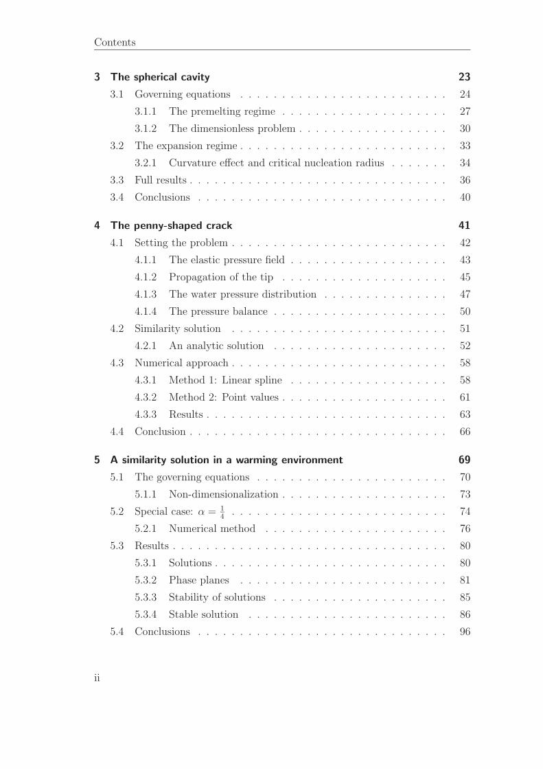
Contents
1 Introduction 1
1.1 The geophysical problem . . . . . . . . . . . . . . . . . . . . . . . 1
1.2 Frost heave . . . . . . . . . . . . . . . . . . . . . . . . . . . . . . 5
1.2.1 Expansion resulting from solidification . . . . . . . . . . . 6
1.2.2 Past studies . . . . . . . . . . . . . . . . . . . . . . . . . . 6
1.3 Frost fracturing of rocks . . . . . . . . . . . . . . . . . . . . . . . 9
1.4 Structure of the thesis . . . . . . . . . . . . . . . . . . . . . . . . 13
2 Background theory 15
2.1 Thermodynamics . . . . . . . . . . . . . . . . . . . . . . . . . . . 15
2.1.1 Pressure melting . . . . . . . . . . . . . . . . . . . . . . . 17
2.1.2 Curvature melting . . . . . . . . . . . . . . . . . . . . . . 18
2.1.3 Premelting dynamics . . . . . . . . . . . . . . . . . . . . . 18
2.1.4 Stefan condition . . . . . . . . . . . . . . . . . . . . . . . . 20
2.2 Darcy flow . . . . . . . . . . . . . . . . . . . . . . . . . . . . . . . 21
i
Contents
3 The spherical cavity 23
3.1 Governing equations . . . . . . . . . . . . . . . . . . . . . . . . . 24
3.1.1 The premelting regime . . . . . . . . . . . . . . . . . . . . 27
3.1.2 The dimensionless problem . . . . . . . . . . . . . . . . . . 30
3.2 The expansion regime . . . . . . . . . . . . . . . . . . . . . . . . . 33
3.2.1 Curvature effect and critical nucleation radius . . . . . . . 34
3.3 Full results . . . . . . . . . . . . . . . . . . . . . . . . . . . . . . . 36
3.4 Conclusions . . . . . . . . . . . . . . . . . . . . . . . . . . . . . . 40
4 The penny-shaped crack 41
4.1 Setting the problem . . . . . . . . . . . . . . . . . . . . . . . . . . 42
4.1.1 The elastic pressure field . . . . . . . . . . . . . . . . . . . 43
4.1.2 Propagation of the tip . . . . . . . . . . . . . . . . . . . . 45
4.1.3 The water pressure distribution . . . . . . . . . . . . . . . 47
4.1.4 The pressure balance . . . . . . . . . . . . . . . . . . . . . 50
4.2 Similarity solution . . . . . . . . . . . . . . . . . . . . . . . . . . 51
4.2.1 An analytic solution . . . . . . . . . . . . . . . . . . . . . 52
4.3 Numerical approach . . . . . . . . . . . . . . . . . . . . . . . . . . 58
4.3.1 Method 1: Linear spline . . . . . . . . . . . . . . . . . . . 58
4.3.2 Method 2: Point values . . . . . . . . . . . . . . . . . . . . 61
4.3.3 Results . . . . . . . . . . . . . . . . . . . . . . . . . . . . . 63
4.4 Conclusion . . . . . . . . . . . . . . . . . . . . . . . . . . . . . . . 66
5 A similarity solution in a warming environment 69
5.1 The governing equations . . . . . . . . . . . . . . . . . . . . . . . 70
5.1.1 Non-dimensionalization . . . . . . . . . . . . . . . . . . . . 73
5.2 Special case: α = 14
. . . . . . . . . . . . . . . . . . . . . . . . . . 74
5.2.1 Numerical method . . . . . . . . . . . . . . . . . . . . . . 76
5.3 Results . . . . . . . . . . . . . . . . . . . . . . . . . . . . . . . . . 80
5.3.1 Solutions . . . . . . . . . . . . . . . . . . . . . . . . . . . . 80
5.3.2 Phase planes . . . . . . . . . . . . . . . . . . . . . . . . . 81
5.3.3 Stability of solutions . . . . . . . . . . . . . . . . . . . . . 85
5.3.4 Stable solution . . . . . . . . . . . . . . . . . . . . . . . . 86
5.4 Conclusions . . . . . . . . . . . . . . . . . . . . . . . . . . . . . . 96
ii
Contents
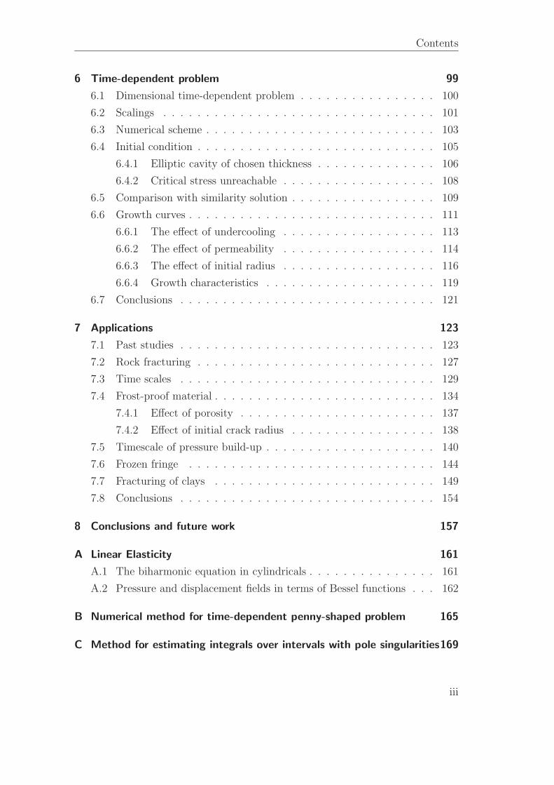
6 Time-dependent problem 99
6.1 Dimensional time-dependent problem . . . . . . . . . . . . . . . . 100
6.2 Scalings . . . . . . . . . . . . . . . . . . . . . . . . . . . . . . . . 101
6.3 Numerical scheme . . . . . . . . . . . . . . . . . . . . . . . . . . . 103
6.4 Initial condition . . . . . . . . . . . . . . . . . . . . . . . . . . . . 105
6.4.1 Elliptic cavity of chosen thickness . . . . . . . . . . . . . . 106
6.4.2 Critical stress unreachable . . . . . . . . . . . . . . . . . . 108
6.5 Comparison with similarity solution . . . . . . . . . . . . . . . . . 109
6.6 Growth curves . . . . . . . . . . . . . . . . . . . . . . . . . . . . . 111
6.6.1 The effect of undercooling . . . . . . . . . . . . . . . . . . 113
6.6.2 The effect of permeability . . . . . . . . . . . . . . . . . . 114
6.6.3 The effect of initial radius . . . . . . . . . . . . . . . . . . 116
6.6.4 Growth characteristics . . . . . . . . . . . . . . . . . . . . 119
6.7 Conclusions . . . . . . . . . . . . . . . . . . . . . . . . . . . . . . 121
7 Applications 123
7.1 Past studies . . . . . . . . . . . . . . . . . . . . . . . . . . . . . . 123
7.2 Rock fracturing . . . . . . . . . . . . . . . . . . . . . . . . . . . . 127
7.3 Time scales . . . . . . . . . . . . . . . . . . . . . . . . . . . . . . 129
7.4 Frost-proof material . . . . . . . . . . . . . . . . . . . . . . . . . . 134
7.4.1 Effect of porosity . . . . . . . . . . . . . . . . . . . . . . . 137
7.4.2 Effect of initial crack radius . . . . . . . . . . . . . . . . . 138
7.5 Timescale of pressure build-up . . . . . . . . . . . . . . . . . . . . 140
7.6 Frozen fringe . . . . . . . . . . . . . . . . . . . . . . . . . . . . . 144
7.7 Fracturing of clays . . . . . . . . . . . . . . . . . . . . . . . . . . 149
7.8 Conclusions . . . . . . . . . . . . . . . . . . . . . . . . . . . . . . 154
8 Conclusions and future work 157
A Linear Elasticity 161
A.1 The biharmonic equation in cylindricals . . . . . . . . . . . . . . . 161
A.2 Pressure and displacement fields in terms of Bessel functions . . . 162
B Numerical method for time-dependent penny-shaped problem 165
C Method for estimating integrals over intervals with pole singularities169
iii
Contents
D Assumption of uniform pressure in the tip of the crack 171
E Freezing temperature depression of a spherical nucleus in a spherical
pore 175
Bibliography 178
iv
Chapter 1
Introduction
1.1 The geophysical problem
Large pressures can develop inside water-saturated porous media at sub-zero tem-
peratures. These pressures can cause fracturing of pre-existing faults, degradation
of rocks and soils, and displacement of the ground surface, and occur due to the
solidification of the water inside the material. The results of such processes are of
interest to both geologists and engineers. Frost-induced deformation of material
can destroy building foundations, damage roads and statues as well as fracture
water supplies and gas and oil pipelines. The importance of freezing in the de-
velopment of landscapes is also widely recognized (Washburn, 1980). When soils
freeze, segregated ice lenses consisting of ice blocks devoid of soil particles form,
which cause upward movement of the ground above. While this process, called
1
1 Introduction
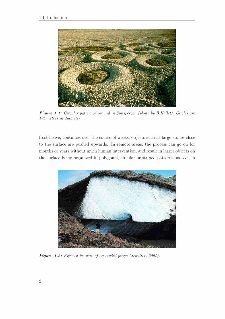
Figure 1.1: Circular patterned ground in Spitspergen (photo by B.Hallet). Circles are1-2 metres in diameter.
frost heave, continues over the course of weeks, objects such as large stones close
to the surface are pushed upwards. In remote areas, the process can go on for
months or years without much human intervention, and result in larger objects on
the surface being organized in polygonal, circular or striped patterns, as seen in
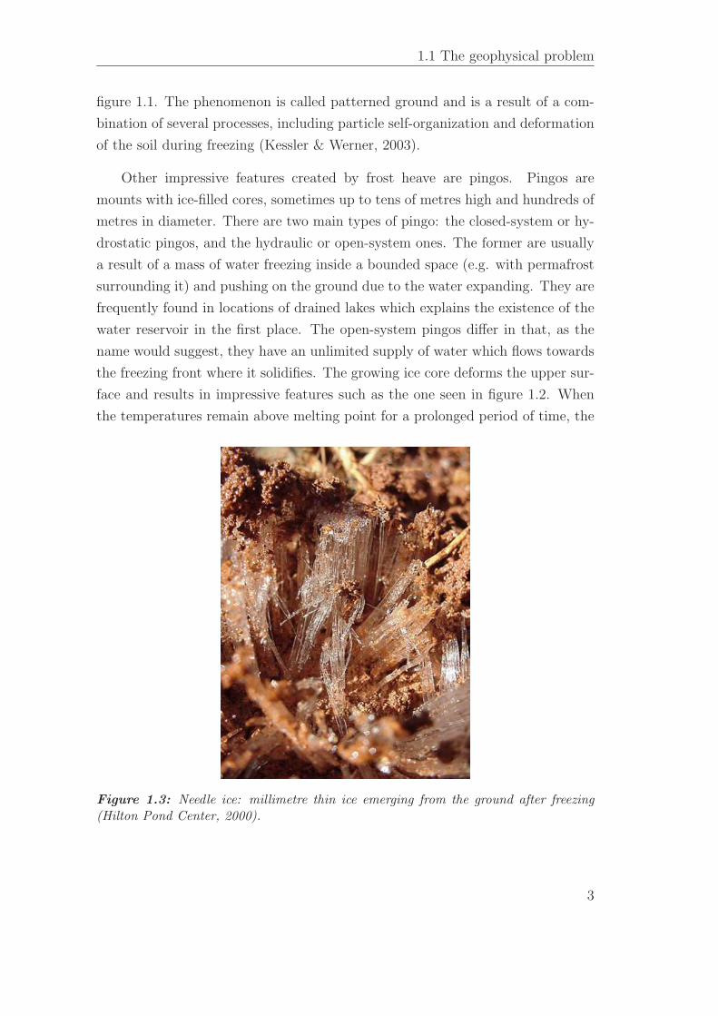
Figure 1.2: Exposed ice core of an eroded pingo (Schutter, 2004).
2
1.1 The geophysical problem
figure 1.1. The phenomenon is called patterned ground and is a result of a com-
bination of several processes, including particle self-organization and deformation
of the soil during freezing (Kessler & Werner, 2003).
Other impressive features created by frost heave are pingos. Pingos are
mounts with ice-filled cores, sometimes up to tens of metres high and hundreds of
metres in diameter. There are two main types of pingo: the closed-system or hy-
drostatic pingos, and the hydraulic or open-system ones. The former are usually
a result of a mass of water freezing inside a bounded space (e.g. with permafrost
surrounding it) and pushing on the ground due to the water expanding. They are
frequently found in locations of drained lakes which explains the existence of the
water reservoir in the first place. The open-system pingos differ in that, as the
name would suggest, they have an unlimited supply of water which flows towards
the freezing front where it solidifies. The growing ice core deforms the upper sur-
face and results in impressive features such as the one seen in figure 1.2. When
the temperatures remain above melting point for a prolonged period of time, the
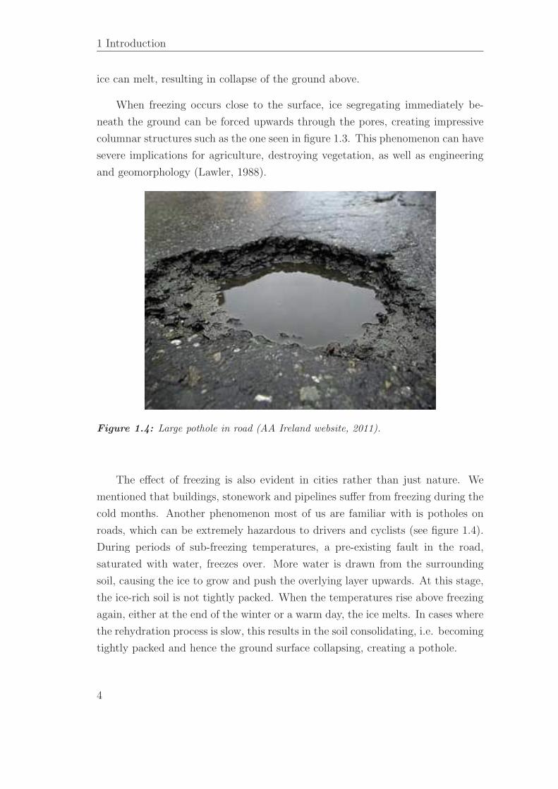
Figure 1.3: Needle ice: millimetre thin ice emerging from the ground after freezing(Hilton Pond Center, 2000).
3
1 Introduction
ice can melt, resulting in collapse of the ground above.
When freezing occurs close to the surface, ice segregating immediately be-
neath the ground can be forced upwards through the pores, creating impressive
columnar structures such as the one seen in figure 1.3. This phenomenon can have
severe implications for agriculture, destroying vegetation, as well as engineering
and geomorphology (Lawler, 1988).
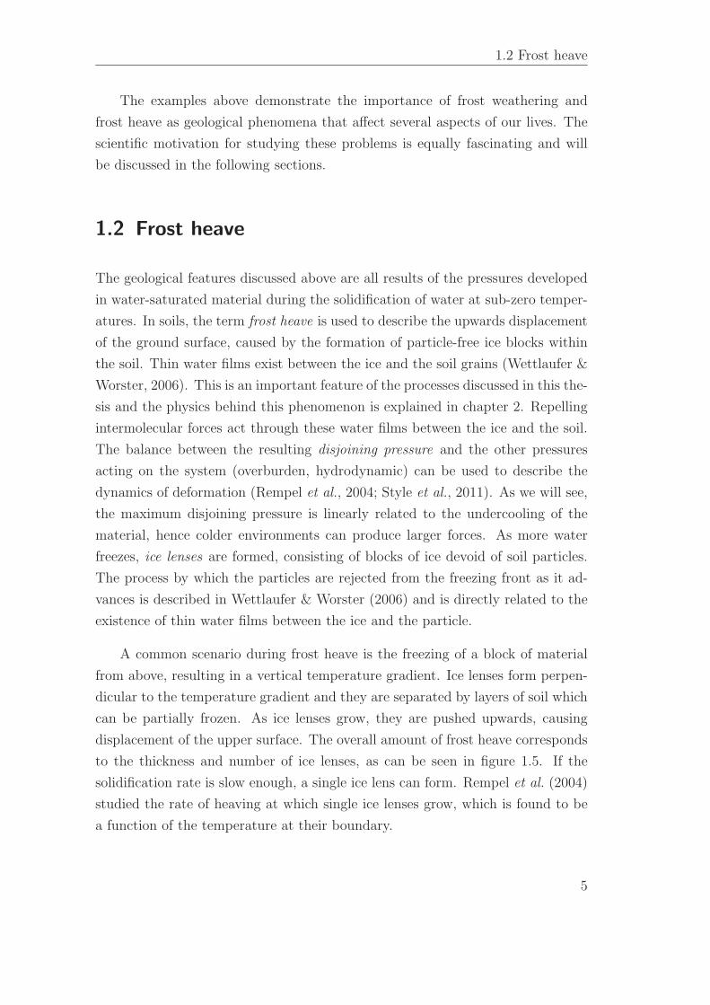
Figure 1.4: Large pothole in road (AA Ireland website, 2011).
The effect of freezing is also evident in cities rather than just nature. We
mentioned that buildings, stonework and pipelines suffer from freezing during the
cold months. Another phenomenon most of us are familiar with is potholes on
roads, which can be extremely hazardous to drivers and cyclists (see figure 1.4).
During periods of sub-freezing temperatures, a pre-existing fault in the road,
saturated with water, freezes over. More water is drawn from the surrounding
soil, causing the ice to grow and push the overlying layer upwards. At this stage,
the ice-rich soil is not tightly packed. When the temperatures rise above freezing
again, either at the end of the winter or a warm day, the ice melts. In cases where
the rehydration process is slow, this results in the soil consolidating, i.e. becoming
tightly packed and hence the ground surface collapsing, creating a pothole.
4
1.2 Frost heave
The examples above demonstrate the importance of frost weathering and
frost heave as geological phenomena that affect several aspects of our lives. The
scientific motivation for studying these problems is equally fascinating and will
be discussed in the following sections.
1.2 Frost heave
The geological features discussed above are all results of the pressures developed
in water-saturated material during the solidification of water at sub-zero temper-
atures. In soils, the term frost heave is used to describe the upwards displacement
of the ground surface, caused by the formation of particle-free ice blocks within
the soil. Thin water films exist between the ice and the soil grains (Wettlaufer &
Worster, 2006). This is an important feature of the processes discussed in this the-
sis and the physics behind this phenomenon is explained in chapter 2. Repelling
intermolecular forces act through these water films between the ice and the soil.
The balance between the resulting disjoining pressure and the other pressures
acting on the system (overburden, hydrodynamic) can be used to describe the
dynamics of deformation (Rempel et al., 2004; Style et al., 2011). As we will see,
the maximum disjoining pressure is linearly related to the undercooling of the
material, hence colder environments can produce larger forces. As more water
freezes, ice lenses are formed, consisting of blocks of ice devoid of soil particles.
The process by which the particles are rejected from the freezing front as it ad-
vances is described in Wettlaufer & Worster (2006) and is directly related to the
existence of thin water films between the ice and the particle.
A common scenario during frost heave is the freezing of a block of material
from above, resulting in a vertical temperature gradient. Ice lenses form perpen-
dicular to the temperature gradient and they are separated by layers of soil which
can be partially frozen. As ice lenses grow, they are pushed upwards, causing
displacement of the upper surface. The overall amount of frost heave corresponds
to the thickness and number of ice lenses, as can be seen in figure 1.5. If the
solidification rate is slow enough, a single ice lens can form. Rempel et al. (2004)
studied the rate of heaving at which single ice lenses grow, which is found to be
a function of the temperature at their boundary.
5
1 Introduction
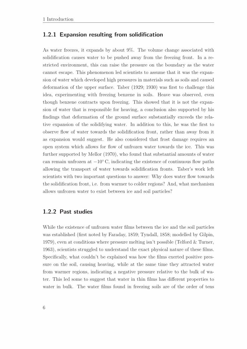
1.2.1 Expansion resulting from solidification
As water freezes, it expands by about 9%. The volume change associated with
solidification causes water to be pushed away from the freezing front. In a re-
stricted environment, this can raise the pressure on the boundary as the water
cannot escape. This phenomenon led scientists to assume that it was the expan-
sion of water which developed high pressures in materials such as soils and caused
deformation of the upper surface. Taber (1929; 1930) was first to challenge this
idea, experimenting with freezing benzene in soils. Heave was observed, even
though benzene contracts upon freezing. This showed that it is not the expan-
sion of water that is responsible for heaving, a conclusion also supported by his
findings that deformation of the ground surface substantially exceeds the rela-
tive expansion of the solidifying water. In addition to this, he was the first to
observe flow of water towards the solidification front, rather than away from it
as expansion would suggest. He also considered that frost damage requires an
open system which allows for flow of unfrozen water towards the ice. This was
further supported by Mellor (1970), who found that substantial amounts of water
can remain unfrozen at −10◦ C, indicating the existence of continuous flow paths
allowing the transport of water towards solidification fronts. Taber’s work left
scientists with two important questions to answer: Why does water flow towards
the solidification front, i.e. from warmer to colder regions? And, what mechanism
allows unfrozen water to exist between ice and soil particles?
1.2.2 Past studies
While the existence of unfrozen water films between the ice and the soil particles
was established (first noted by Faraday, 1859; Tyndall, 1858; modelled by Gilpin,
1979), even at conditions where pressure melting isn’t possible (Telford & Turner,
1963), scientists struggled to understand the exact physical nature of these films.
Specifically, what couldn’t be explained was how the films exerted positive pres-
sure on the soil, causing heaving, while at the same time they attracted water
from warmer regions, indicating a negative pressure relative to the bulk of wa-
ter. This led some to suggest that water in thin films has different properties to
water in bulk. The water films found in freezing soils are of the order of tens
6
1.2 Frost heave
of nanometres, which made it difficult to gather experimental evidence on wa-
ter properties directly. Vignes-Adler (1977) suggested that the pressure tensor
in thin water films is anisotropic, with an additional pressure component, the
“extrastress”, which acts only across the film and is interpreted as the disjoining
pressure responsible for the deformation of the soil.
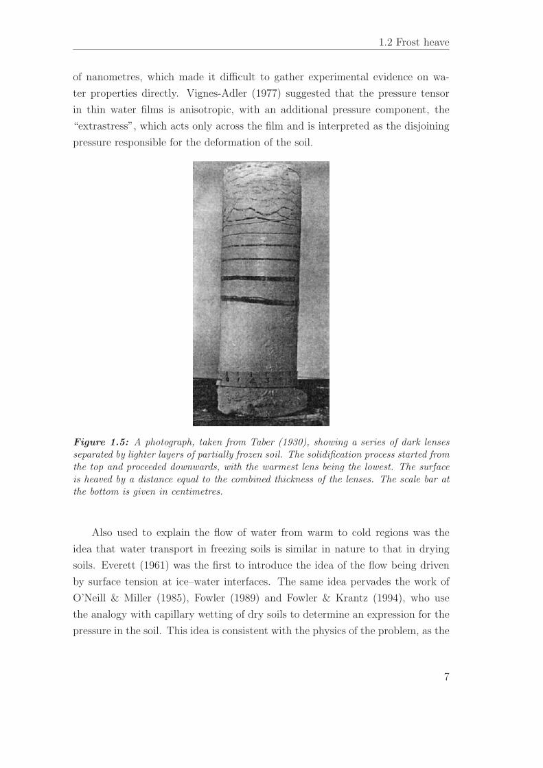
Figure 1.5: A photograph, taken from Taber (1930), showing a series of dark lensesseparated by lighter layers of partially frozen soil. The solidification process started fromthe top and proceeded downwards, with the warmest lens being the lowest. The surfaceis heaved by a distance equal to the combined thickness of the lenses. The scale bar atthe bottom is given in centimetres.
Also used to explain the flow of water from warm to cold regions was the
idea that water transport in freezing soils is similar in nature to that in drying
soils. Everett (1961) was the first to introduce the idea of the flow being driven
by surface tension at ice–water interfaces. The same idea pervades the work of
O’Neill & Miller (1985), Fowler (1989) and Fowler & Krantz (1994), who use
the analogy with capillary wetting of dry soils to determine an expression for the
pressure in the soil. This idea is consistent with the physics of the problem, as the
7
1 Introduction
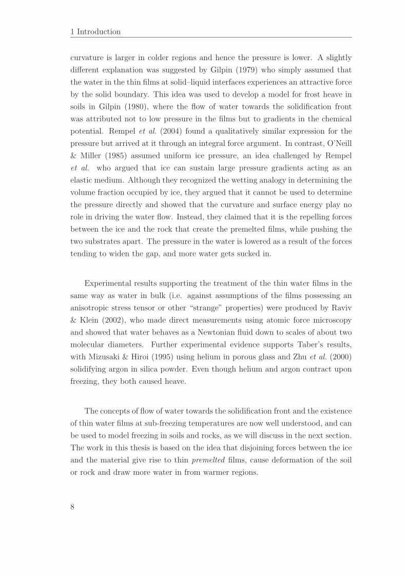
curvature is larger in colder regions and hence the pressure is lower. A slightly
different explanation was suggested by Gilpin (1979) who simply assumed that
the water in the thin films at solid–liquid interfaces experiences an attractive force
by the solid boundary. This idea was used to develop a model for frost heave in
soils in Gilpin (1980), where the flow of water towards the solidification front
was attributed not to low pressure in the films but to gradients in the chemical
potential. Rempel et al. (2004) found a qualitatively similar expression for the
pressure but arrived at it through an integral force argument. In contrast, O’Neill
& Miller (1985) assumed uniform ice pressure, an idea challenged by Rempel
et al. who argued that ice can sustain large pressure gradients acting as an
elastic medium. Although they recognized the wetting analogy in determining the
volume fraction occupied by ice, they argued that it cannot be used to determine
the pressure directly and showed that the curvature and surface energy play no
role in driving the water flow. Instead, they claimed that it is the repelling forces
between the ice and the rock that create the premelted films, while pushing the
two substrates apart. The pressure in the water is lowered as a result of the forces
tending to widen the gap, and more water gets sucked in.
Experimental results supporting the treatment of the thin water films in the
same way as water in bulk (i.e. against assumptions of the films possessing an
anisotropic stress tensor or other “strange” properties) were produced by Raviv
& Klein (2002), who made direct measurements using atomic force microscopy
and showed that water behaves as a Newtonian fluid down to scales of about two
molecular diameters. Further experimental evidence supports Taber’s results,
with Mizusaki & Hiroi (1995) using helium in porous glass and Zhu et al. (2000)
solidifying argon in silica powder. Even though helium and argon contract upon
freezing, they both caused heave.
The concepts of flow of water towards the solidification front and the existence
of thin water films at sub-freezing temperatures are now well understood, and can
be used to model freezing in soils and rocks, as we will discuss in the next section.
The work in this thesis is based on the idea that disjoining forces between the ice
and the material give rise to thin premelted films, cause deformation of the soil
or rock and draw more water in from warmer regions.
8
1.3 Frost fracturing of rocks
1.3 Frost fracturing of rocks
When water in rocks freezes, large pressures develop which can cause consid-
erable damage to the rock. As discussed at the beginning of the introduction,
this phenomenon has important consequences as it affects buildings, statues and
pipelines, as well as contributing to landscape development.
It is natural to expect that frost fracturing is governed by similar mechanisms
to frost heave. The connection is made through the assumption that ice-filled
cavities in rocks play the role of ice lenses in soils. Similarly to soils, the early
assumption about the cause of frost weathering of rocks was the expansion of
water by 9% during solidification. This is the core of the volumetric-expansion
model applied to porous rocks, and it implies that no fracturing can take place
in a rock saturated with a fluid that contracts upon freezing. Many scientists
used this model to try to explain frost weathering. As noted by Walder & Hallet
(1985), several publications (see Embleton & King, 1975; Washburn, 1980; Tharp,
1983) considered volumetric expansion in sealed cracks the cause of damage to
rocks. Although this is physically consistent, as the pressure build-up from the
expansion would be considerable if the water had no means of escaping, it poses
the question of how a sealed crack can be filled with water in the first place. The
scenario would be relevant for a saturated rock being rapidly cooled from the
outside from all sides, but its applications are limited.
The volumetric-expansion model is dependent on the idea that water is forced
away from the solidification front and raises the pressure inside the medium, as the
space that can be occupied by water is limited. This requires the medium to be
completely (or, at least, considerably) saturated with water. If a large proportion
of the pores were empty, the water would simply fill them and the pressure would
be relaxed. Defining the saturation level as the percentage of the rock pores
filled with water, and remembering that freezing water expands by about 9%, we
see that a minimum saturation level of 91% would be required for fracturing to
occur. This value hasn’t been verified experimentally. For example, McGreevy
& Whalley (1985) reported fracturing even for rocks only about 80% saturated
but attributed the inaccuracy to heterogeneities in water concentration, which
would make the accurate calculation of moisture levels difficult. Murton et al.
9
1 Introduction
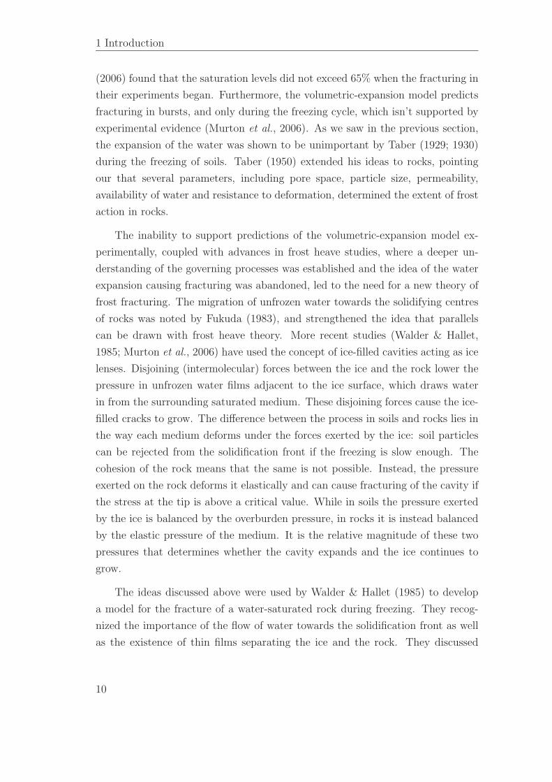
(2006) found that the saturation levels did not exceed 65% when the fracturing in
their experiments began. Furthermore, the volumetric-expansion model predicts
fracturing in bursts, and only during the freezing cycle, which isn’t supported by
experimental evidence (Murton et al., 2006). As we saw in the previous section,
the expansion of the water was shown to be unimportant by Taber (1929; 1930)
during the freezing of soils. Taber (1950) extended his ideas to rocks, pointing
our that several parameters, including pore space, particle size, permeability,
availability of water and resistance to deformation, determined the extent of frost
action in rocks.
The inability to support predictions of the volumetric-expansion model ex-
perimentally, coupled with advances in frost heave studies, where a deeper un-
derstanding of the governing processes was established and the idea of the water
expansion causing fracturing was abandoned, led to the need for a new theory of
frost fracturing. The migration of unfrozen water towards the solidifying centres
of rocks was noted by Fukuda (1983), and strengthened the idea that parallels
can be drawn with frost heave theory. More recent studies (Walder & Hallet,
1985; Murton et al., 2006) have used the concept of ice-filled cavities acting as ice
lenses. Disjoining (intermolecular) forces between the ice and the rock lower the
pressure in unfrozen water films adjacent to the ice surface, which draws water
in from the surrounding saturated medium. These disjoining forces cause the ice-
filled cracks to grow. The difference between the process in soils and rocks lies in
the way each medium deforms under the forces exerted by the ice: soil particles
can be rejected from the solidification front if the freezing is slow enough. The
cohesion of the rock means that the same is not possible. Instead, the pressure
exerted on the rock deforms it elastically and can cause fracturing of the cavity if
the stress at the tip is above a critical value. While in soils the pressure exerted
by the ice is balanced by the overburden pressure, in rocks it is instead balanced
by the elastic pressure of the medium. It is the relative magnitude of these two
pressures that determines whether the cavity expands and the ice continues to
grow.
The ideas discussed above were used by Walder & Hallet (1985) to develop
a model for the fracture of a water-saturated rock during freezing. They recog-
nized the importance of the flow of water towards the solidification front as well
as the existence of thin films separating the ice and the rock. They discussed
10
1.3 Frost fracturing of rocks
how these films exert an “attractive force” on the pore water (hence the flow
towards the ice front) and a disjoining pressure that pushes the ice and the rock
apart. They showed that the fastest growth rate occurs at temperatures in the
range −4 to −15◦C as, in colder systems, the transport of water is limited ow-
ing to the large amount of pore ice reducing the permeability of the rock. For
temperatures closer to 0◦C, the maximum disjoining pressure (linearly related to
the undercooling) is not large enough to cause the stress at the tip of the crack
to exceed the “stress–corrosion” limit, the value above which Walder & Hallet
predict fracturing. A similar fracture model was used by Murton et al. (2006)
for their numerical simulations, coupled with a more complicated mass and heat
transfer model.
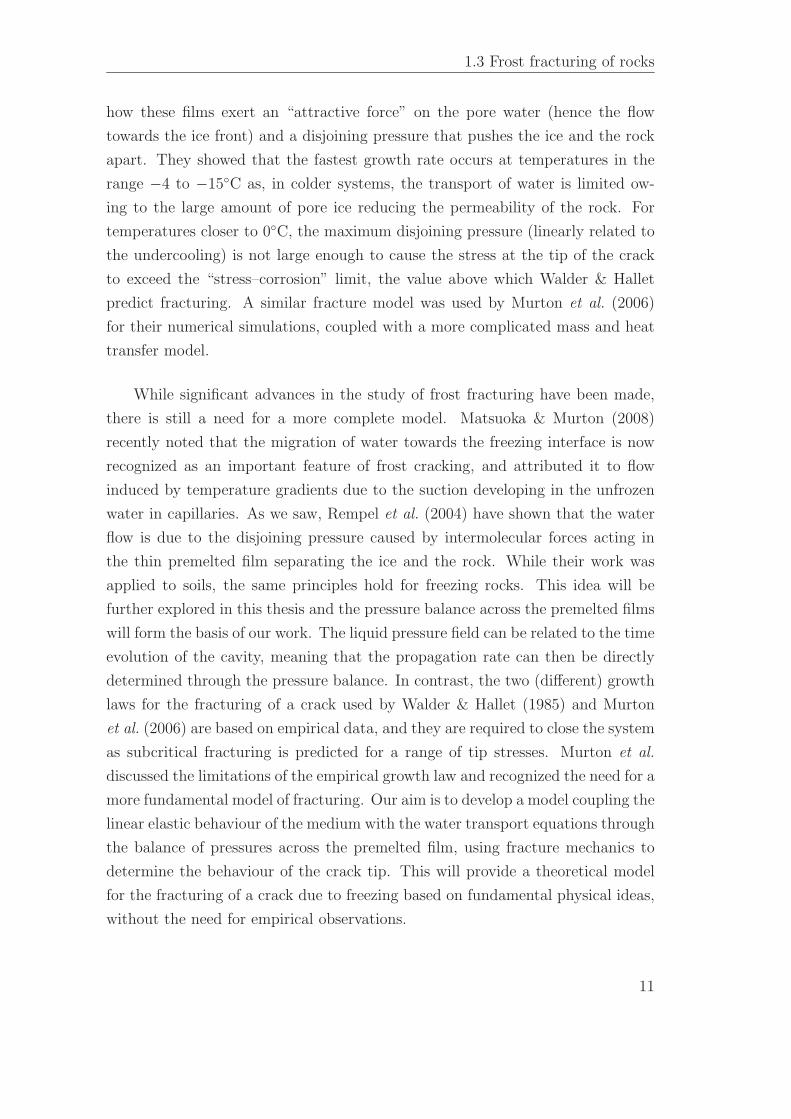
While significant advances in the study of frost fracturing have been made,
there is still a need for a more complete model. Matsuoka & Murton (2008)
recently noted that the migration of water towards the freezing interface is now
recognized as an important feature of frost cracking, and attributed it to flow
induced by temperature gradients due to the suction developing in the unfrozen
water in capillaries. As we saw, Rempel et al. (2004) have shown that the water
flow is due to the disjoining pressure caused by intermolecular forces acting in
the thin premelted film separating the ice and the rock. While their work was
applied to soils, the same principles hold for freezing rocks. This idea will be
further explored in this thesis and the pressure balance across the premelted films
will form the basis of our work. The liquid pressure field can be related to the time
evolution of the cavity, meaning that the propagation rate can then be directly
determined through the pressure balance. In contrast, the two (different) growth
laws for the fracturing of a crack used by Walder & Hallet (1985) and Murton
et al. (2006) are based on empirical data, and they are required to close the system
as subcritical fracturing is predicted for a range of tip stresses. Murton et al.
discussed the limitations of the empirical growth law and recognized the need for a
more fundamental model of fracturing. Our aim is to develop a model coupling the
linear elastic behaviour of the medium with the water transport equations through
the balance of pressures across the premelted film, using fracture mechanics to
determine the behaviour of the crack tip. This will provide a theoretical model
for the fracturing of a crack due to freezing based on fundamental physical ideas,
without the need for empirical observations.
11
1 Introduction
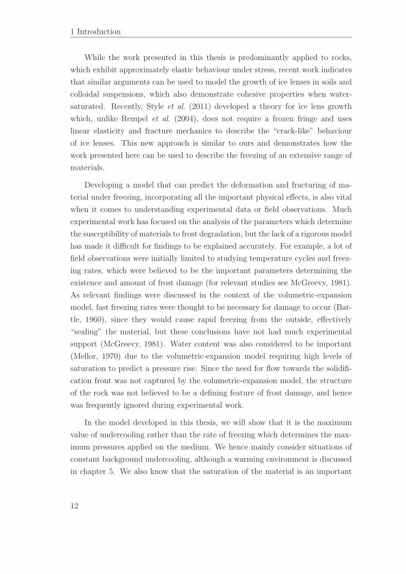
While the work presented in this thesis is predominantly applied to rocks,
which exhibit approximately elastic behaviour under stress, recent work indicates
that similar arguments can be used to model the growth of ice lenses in soils and
colloidal suspensions, which also demonstrate cohesive properties when water-
saturated. Recently, Style et al. (2011) developed a theory for ice lens growth
which, unlike Rempel et al. (2004), does not require a frozen fringe and uses
linear elasticity and fracture mechanics to describe the “crack-like” behaviour
of ice lenses. This new approach is similar to ours and demonstrates how the
work presented here can be used to describe the freezing of an extensive range of
materials.
Developing a model that can predict the deformation and fracturing of ma-
terial under freezing, incorporating all the important physical effects, is also vital
when it comes to understanding experimental data or field observations. Much
experimental work has focused on the analysis of the parameters which determine
the susceptibility of materials to frost degradation, but the lack of a rigorous model
has made it difficult for findings to be explained accurately. For example, a lot of
field observations were initially limited to studying temperature cycles and freez-
ing rates, which were believed to be the important parameters determining the
existence and amount of frost damage (for relevant studies see McGreevy, 1981).
As relevant findings were discussed in the context of the volumetric-expansion
model, fast freezing rates were thought to be necessary for damage to occur (Bat-
tle, 1960), since they would cause rapid freezing from the outside, effectively
“sealing” the material, but these conclusions have not had much experimental
support (McGreevy, 1981). Water content was also considered to be important
(Mellor, 1970) due to the volumetric-expansion model requiring high levels of
saturation to predict a pressure rise. Since the need for flow towards the solidifi-
cation front was not captured by the volumetric-expansion model, the structure
of the rock was not believed to be a defining feature of frost damage, and hence
was frequently ignored during experimental work.
In the model developed in this thesis, we will show that it is the maximum
value of undercooling rather than the rate of freezing which determines the max-
imum pressures applied on the medium. We hence mainly consider situations of
constant background undercooling, although a warming environment is discussed
in chapter 5. We also know that the saturation of the material is an important
12
1.4 Structure of the thesis
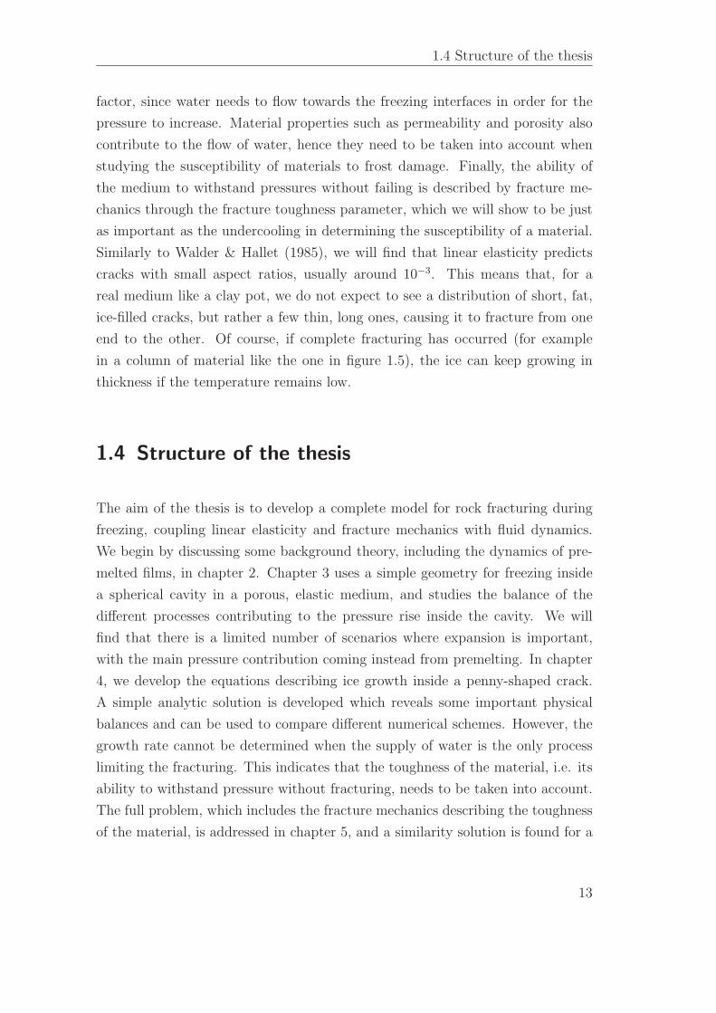
factor, since water needs to flow towards the freezing interfaces in order for the
pressure to increase. Material properties such as permeability and porosity also
contribute to the flow of water, hence they need to be taken into account when
studying the susceptibility of materials to frost damage. Finally, the ability of
the medium to withstand pressures without failing is described by fracture me-
chanics through the fracture toughness parameter, which we will show to be just
as important as the undercooling in determining the susceptibility of a material.
Similarly to Walder & Hallet (1985), we will find that linear elasticity predicts
cracks with small aspect ratios, usually around 10−3. This means that, for a
real medium like a clay pot, we do not expect to see a distribution of short, fat,
ice-filled cracks, but rather a few thin, long ones, causing it to fracture from one
end to the other. Of course, if complete fracturing has occurred (for example
in a column of material like the one in figure 1.5), the ice can keep growing in
thickness if the temperature remains low.
1.4 Structure of the thesis
The aim of the thesis is to develop a complete model for rock fracturing during
freezing, coupling linear elasticity and fracture mechanics with fluid dynamics.
We begin by discussing some background theory, including the dynamics of pre-
melted films, in chapter 2. Chapter 3 uses a simple geometry for freezing inside
a spherical cavity in a porous, elastic medium, and studies the balance of the
different processes contributing to the pressure rise inside the cavity. We will
find that there is a limited number of scenarios where expansion is important,
with the main pressure contribution coming instead from premelting. In chapter
4, we develop the equations describing ice growth inside a penny-shaped crack.
A simple analytic solution is developed which reveals some important physical
balances and can be used to compare different numerical schemes. However, the
growth rate cannot be determined when the supply of water is the only process
limiting the fracturing. This indicates that the toughness of the material, i.e. its
ability to withstand pressure without fracturing, needs to be taken into account.
The full problem, which includes the fracture mechanics describing the toughness
of the material, is addressed in chapter 5, and a similarity solution is found for a
13

1 Introduction
special case of the environment warming according to a power law in time. While
restricting the boundary conditions in this way limits the applicability of the re-
sults, the qualitative ideas we develop are extremely useful as we gain a deeper
understanding of the dependence of fracturing on the different parameters of the
problem. The full time-dependent problem is solved numerically in chapter 6 and
the growth rate characteristics of a crack are analysed. The initial stage of ice
build-up is also discussed, and the conditions required for a pre-existing fault to
fracture are determined. Chapter 7 involves further analysis of the penny-shaped
model, and a comparison with existing numerical data from other models. The
susceptibility of different materials to frost-induced degradation is analysed. The
model is also extended to include the effect of pore ice on the permeability of
the medium, which can be important at low temperatures as it limits the water
supply. Finally, we show how the model is suitable to describe ice lens formation
in clays and soils.
14
Chapter 2
Background theory
The aim of this chapter is to introduce the main background ideas which govern
the work presented in this thesis. The thermodynamics of the problem are dis-
cussed, and the equations which govern the freezing temperature and the heat
release during solidification are derived. We also present the physics of the pre-
melted films between rock and ice, which give us the pressure balance across them,
as well as the equations for Darcy flow through the porous medium, which will
be used to determine the liquid pressure field.
2.1 Thermodynamics
Classical thermodynamics can be used to describe the process of solidification,
i.e. the change of state from liquid to solid. The melting/freezing point is defined
15
2 Background theory
as the temperature at which the liquid and the solid phases can coexist. This
temperature, Tm, is measured at a certain reference pressure pm as it is affected
by changes in pressure.
We first define some quantities that will be used to derive some basic equations
relevant to the work in later chapters. The specific enthalpy H describes the
energy of the system
H = U + pV, (2.1)
where U is the specific internal energy, p the pressure and V = ρ−1 the specific
volume. Changes in the specific enthalpy H arise either from a change in the
specific entropy S of the system or a change in pressure
dH = TdS + V dp. (2.2)
The specific energy available by the system for useful work is described by the
specific Gibbs free energy
G = H − ST (2.3)
hence a change in G can be expressed as
dG = dH − SdT − TdS = V dp − SdT. (2.4)
At a phase boundary in equilibrium, G is the same in the two phases, Gs = Gl.
Hence, applying this at the reference state (Tm, pm), equation (2.3) gives
Hl − Hs = (Sl − Ss)Tm ≡ L (2.5)
where L is the latent heat required to convert a unit mass of a solid into liquid
at the melting temperature Tm.
The specific Gibbs free energy of the liquid, Gl, is equal to that of the solid,
Gs, when the two phases coexist. Any change of temperature and pressure that
preserves the phase coexistence, will have
dGl = dGs. (2.6)
By considering small departures from a reference state (Tm, pm) to a state that
has (T, ps) in the solid state and (T, pl) at the liquid state (since the temperature
16
2.1 Thermodynamics
is continuous across the boundary), and using equation (2.4) we find
Vs(ps − pm) − Ss(T − Tm) = Vl(pl − pm) − Sl(T − Tm). (2.7)
Re-arranging the expression above for Sl−Ss and using the definition of the latent
heat L, we can re-write it as
ρsLTm − T
Tm
= (ps − pl) + (pl − pm)
(
1 − ρs
ρl
)
, (2.8)
which is known as the Gibbs-Duhem equation (Reif, 1965). The densities of the
solid and liquid state are ρs and ρl respectively. This equation describes the effect
that a difference of pressures across the liquid–solid interface (first term on right-
hand-side of equation) or a change from the reference pressure pm (second term
of right-hand-side of equation) have on the freezing temperature of a substance.
Next, we look at how each of the two terms can cause a change in the freezing
temperature.
2.1.1 Pressure melting
Across a planar interface the liquid and solid pressures are equal, pl = ps = p,
say. In that case, equation (2.8) can be differentiated to show that
dp
dT= − ρsρlL
Tm ∆ρ, (2.9)
where ∆ρ = ρl − ρs. This is known as the Clausius-Clapeyron equation and
describes the effect of pressure on the melting temperature of a substance. Liquids
that are denser in the solid state, i.e. contract upon freezing, solidify at a higher
temperature under pressure because the pressure helps to hold the molecules
together. However, water is special in that it expands when it freezes (ρl > ρs).
An increased pressure, trying to compress it, causes it to remain in the liquid
state. Similarly, increased pressure on ice causes melting by lowering the freezing
temperature. This phenomenon is called pressure melting.
17
2 Background theory
2.1.2 Curvature melting
A phase boundary with curvature κ = ∇.n, where n is the normal pointing into
the liquid, experiences a difference in the pressure of the solid and liquid phase
on either side of it, caused by the surface tension
ps − pl = κγ, (2.10)
where γ is the surface energy per unit area. If we take the reference pressure to
be that in the liquid state in (2.8), i.e. pl = pm, we find
ρsLTm − T
Tm
= κγ, (2.11)
which describes the effect of curvature on the melting temperature of a solid–
liquid interface, known as the Gibbs-Thompson effect. While we will see that this
is negligible in comparison to the effect of premelting (see section 2.1.3), it will
play an important role in some cases described in chapters 5 and 6.
2.1.3 Premelting dynamics
The definition of the melting temperature Tm implies that at temperatures T <
Tm, the bulk of a mass of substance remains in the solid state. The process
of melting begins at the surface and here we will discuss how that can occur
at T < Tm. We have already discussed the Gibbs-Thompson effect, where the
freezing temperature is depressed on a curved surface and films of melt can exist
on the surface at temperatures below the melting point Tm.
Similar effects can be observed on the boundaries of solids due to intermolec-
ular interactions with the bounding material. The term interfacial premelting
describes the existence of these microscopic films of melt on the surfaces of sub-
stances which are frozen in bulk, at temperatures below the melting temperature
of the substance. These films can occur either at the vapour interface (surface
melting), against a foreign substrate (interfacial melting) or at the interface be-
tween two crystallites of the same substance (grain-boundary melting) as de-
scribed in Wettlaufer & Worster (2006). Interfacial premelting can be induced
18
2.1 Thermodynamics
by a variety of intermolecular forces. Here, we will consider the case of van der
Waals forces as a specific example and concentrate on interfacial melting, where
the solid is bounded by a foreign substrate, since this is the type of situation that
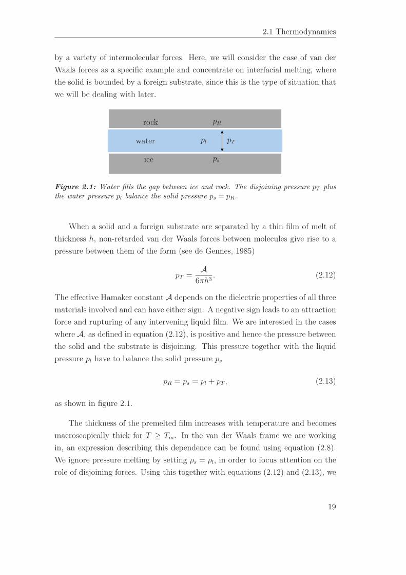
we will be dealing with later.
ps
pl
pR
pTwater
ice
rock
Figure 2.1: Water fills the gap between ice and rock. The disjoining pressure pT plusthe water pressure pl balance the solid pressure ps = pR.
When a solid and a foreign substrate are separated by a thin film of melt of
thickness h, non-retarded van der Waals forces between molecules give rise to a
pressure between them of the form (see de Gennes, 1985)
pT =A
6πh3. (2.12)
The effective Hamaker constant A depends on the dielectric properties of all three
materials involved and can have either sign. A negative sign leads to an attraction
force and rupturing of any intervening liquid film. We are interested in the cases
where A, as defined in equation (2.12), is positive and hence the pressure between
the solid and the substrate is disjoining. This pressure together with the liquid
pressure pl have to balance the solid pressure ps
pR = ps = pl + pT , (2.13)
as shown in figure 2.1.
The thickness of the premelted film increases with temperature and becomes
macroscopically thick for T ≥ Tm. In the van der Waals frame we are working
in, an expression describing this dependence can be found using equation (2.8).
We ignore pressure melting by setting ρs = ρl, in order to focus attention on the
role of disjoining forces. Using this together with equations (2.12) and (2.13), we
19
2 Background theory
then find that the equilibrium thickness of the premelted liquid film is given by
h =
( ATm
6πρsL∆T
)1/3
. (2.14)
The Hamaker constant for rock–water–ice interfaces is in the region of A = 10−18−10−21 J (Watanabe & Flury, 2008). For an undercooling of ∆T = 1 K, this results
in a premelted film of thickness of the order of 10 nm.
This variation in the film thickness gives rise to many interesting phenomena
where there is a temperature variation imposed. Examples include thermody-
namic buoyancy and thermal regelation where a foreign particle in ice that is
subjected to a uniform temperature gradient ∇T experiences a net force simi-
lar to a thermodynamic buoyancy force and moves up the temperature gradient
(Rempel, Wettlaufer & Worster, 2001). Materials confined within capillary tubes
premelt against the boundaries and when imposed to temperature gradients, they
can cause large deformation over a small region towards the cold end of the capil-
lary (Wettlaufer & Worster, 1995). Marangoni-like flows along thin films of water
on ice surfaces are caused by the thermomolecular disjoining pressure and have
been studied by Wettlaufer & Worster (2006).
2.1.4 Stefan condition
In a system with an unlimited supply of liquid, the freezing rate is simply deter-
mined by the temperature field, as temperature gradients determine the rate of
transport of heat away from the solidification front. During a change of phase,
energy called latent heat is released or absorbed by the object. When water so-
lidifies, moving molecules become incorporated in the solid lattice and lose their
entropy. This causes the release of latent heat of fusion which has to be trans-
ported away in order for the process to continue. This balance of heat is described
by the Stefan condition (e.g. Worster, 2000), which states that the rate of release
of latent heat per unit area is equal to the net heat flux away from the interface,
i.e.
ρsLVn = n.ql − n.qs, (2.15)
20
2.2 Darcy flow
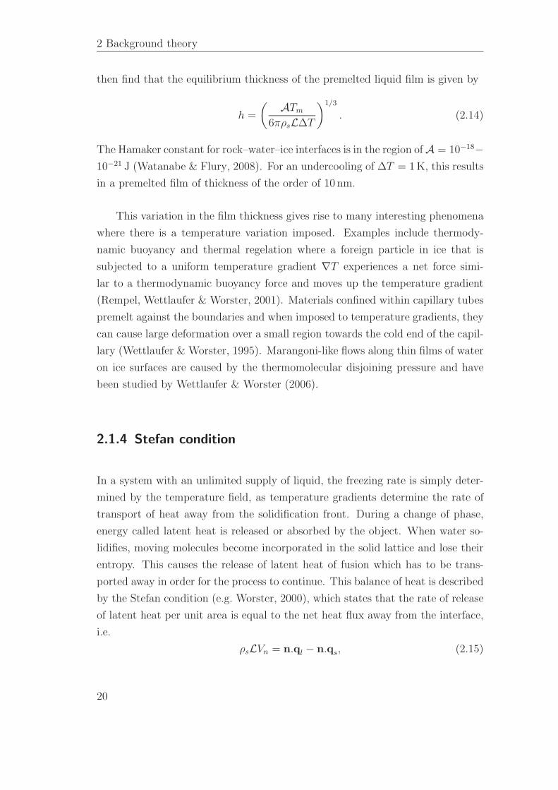
Vn
qs
ql
n
t + δtt
Liquid
Solid
Figure 2.2: Diagram explaining the balance of heat across the solidifying interface.The latent heat released per unit area in time δt is ρsLδt while the heat transportedaway is (n.ql − n.qs)δt.
where ks,l is the thermal conductivity of the corresponding material and qs,l =
−ks,l∇T , evaluated on the freezing boundary, is the local heat flux vector in the
solid and liquid phases respectively. The local rate of solidification is denoted by
Vn as seen in figure 2.2, and L is the latent heat per unit mass.
2.2 Darcy flow
As we saw in the introduction, a lot of discussion has been based around the flow
of water through the porous medium during frost heave or frost fracturing. While
expansion predicts flow of water away from the solidification front, experiments
have indicated that the flow is reversed, from the porous medium towards the ice
(see chapter 1 for more details). In either case, it is important to understand the
equations describing the flow through the rock or soil.
The flow through a porous medium is described by the equation derived by
Darcy, relating the flux per unit area to the pressure gradient. Only a fraction
of the total volume is free for water to flow through it, hence it makes sense to
use an averaged value of the velocity. We use the symbol u for the Darcy flux,
which has units of length per time, for consistency with the flow of water inside
a cavity, as we will see in chapter 3. The real velocity of the water through the
21
2 Background theory
pores can be related to the Darcy flux through the porosity φ of the medium
upore =u
φ. (2.16)
The Darcy equation for flow through the porous medium is
µu = −Π∇p, (2.17)
where p is the pressure, µ the viscosity and Π the permeability of the porous
medium. The mass continuity is the second equation describing the flow
∇.u = 0 (2.18)
and, used together with equation (2.17), gives a useful equation for the pressure
of the water
∇2p = 0. (2.19)
As we are interested in obtaining an expression for the liquid pressure inside the
premelted film, an important part of solving the problems presented in the next
chapters will be to derive a solution to Laplace’s equation (2.19) for the relevant
geometries.
22
Chapter 3
The spherical cavity
As discussed in the introduction of this thesis, the physical mechanisms of frost
fracturing are not very well understood and no complete mathematical model
exists. In particular, while experiments (Taber, 1929; 1930; Mizusaki & Hiroi,
1995; Zhu et al., 2000) have shown that the expansion of the freezing liquid is not
a necessary condition for fracturing, several studies assumed that large pressures
develop owing to the increasing volume of ice. In reality, both expansion and
premelting can cause large pressures inside rocks. The aim of this chapter is to
create a simple model that incorporates both features and allows us to compare
the relative magnitude of their effects.
The two regimes are characterized by contrasting features. When expansion
dominates, water flows away from the freezing front and into the medium. In
contrast, when premelting is important, the flow reverses. We will attempt to
23
3 The spherical cavity
reproduce these features. We shall find that the effect of expansion is negligible
in most cases. Therefore, when we want to restrict attention to the effect of
disjoining forces we ignore expansion by setting the density of the ice ρs equal to
the density of the water ρl. We concentrate on the physical mechanisms associated
with disjoining pressure, modelling it based on van der Waals forces, and show
that it has to balance the pressure difference between the ice and the water. The
results of this study give us a useful insight into the mechanisms that are involved
in the fracturing of rocks and how they contribute to the pressure fields within
rocks and ice-filled cavities within them.
3.1 Governing equations
As a means to illustrate and understand the different physical mechanisms in-
volved when ice forms inside a cavity of a porous, elastic rock, we start by con-
sidering the geometrically simple case of a spherical cavity of radius R(t), as
illustrated in Figure 3.1. We consider a system supercooled to some uniform tem-
perature T∞ < Tm, where Tm is the melting temperature of the ice measured at
pressure pm = p∞. We are interested in finding out how the radius of the solid
ice and the pressure in the cavity evolve with time and also how the different
parameters of the problem affect the solidification process.
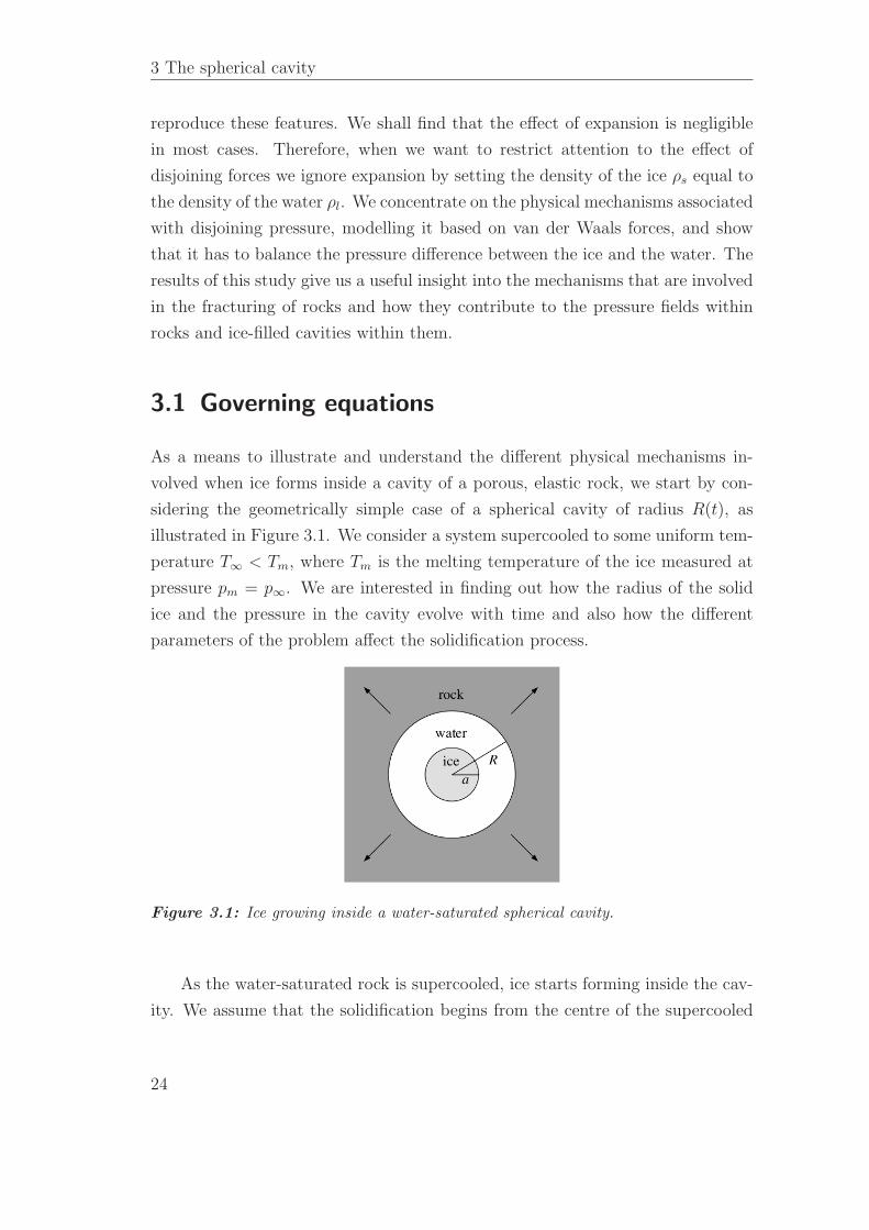
Figure 3.1: Ice growing inside a water-saturated spherical cavity.
As the water-saturated rock is supercooled, ice starts forming inside the cav-
ity. We assume that the solidification begins from the centre of the supercooled
24
3.1 Governing equations
cavity and that the solid ice grows as a sphere of radius a(t). As the water freezes
it expands, causing water to flow away from the solidification front, as shown in
figure 3.1. The water tries to escape the cavity through the porous medium in
which the flow is controlled by the permeability. Flow through the porous medium
requires a pressure gradient which can be substantial if the permeability of the
medium is low. This results in a pressure increase in the cavity, which depresses
the freezing temperature. This process describes how the flow through the porous
medium controls the rate of solidification. We assume the flow in the cavity is
slow, and the temperature field is quasi-steady (see Davis, 2001, pg. 26-29) so
that
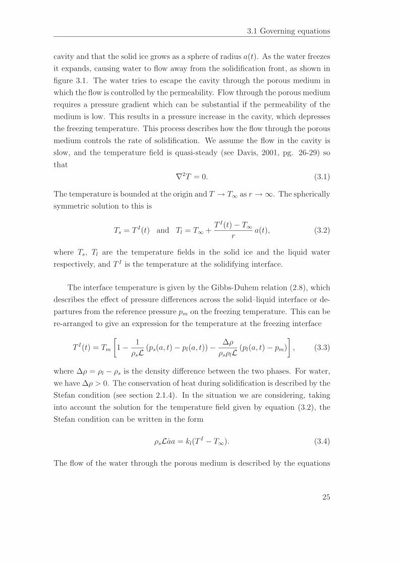
∇2T = 0. (3.1)
The temperature is bounded at the origin and T → T∞ as r → ∞. The spherically
symmetric solution to this is
Ts = T I(t) and Tl = T∞ +T I(t) − T∞
ra(t), (3.2)
where Ts, Tl are the temperature fields in the solid ice and the liquid water
respectively, and T I is the temperature at the solidifying interface.
The interface temperature is given by the Gibbs-Duhem relation (2.8), which
describes the effect of pressure differences across the solid–liquid interface or de-
partures from the reference pressure pm on the freezing temperature. This can be
re-arranged to give an expression for the temperature at the freezing interface
T I(t) = Tm
[
1 − 1
ρsL(ps(a, t) − pl(a, t)) − ∆ρ
ρsρlL(pl(a, t) − pm)
]
, (3.3)
where ∆ρ = ρl − ρs is the density difference between the two phases. For water,
we have ∆ρ > 0. The conservation of heat during solidification is described by the
Stefan condition (see section 2.1.4). In the situation we are considering, taking
into account the solution for the temperature field given by equation (3.2), the
Stefan condition can be written in the form
ρsLaa = kl(TI − T∞). (3.4)
The flow of the water through the porous medium is described by the equations
25
3 The spherical cavity
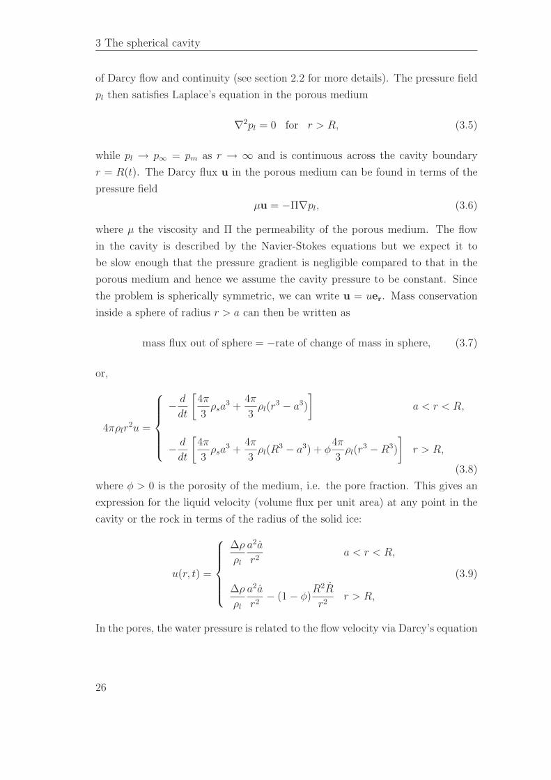
of Darcy flow and continuity (see section 2.2 for more details). The pressure field
pl then satisfies Laplace’s equation in the porous medium
∇2pl = 0 for r > R, (3.5)
while pl → p∞ = pm as r → ∞ and is continuous across the cavity boundary
r = R(t). The Darcy flux u in the porous medium can be found in terms of the
pressure field
µu = −Π∇pl, (3.6)
where µ the viscosity and Π the permeability of the porous medium. The flow
in the cavity is described by the Navier-Stokes equations but we expect it to
be slow enough that the pressure gradient is negligible compared to that in the
porous medium and hence we assume the cavity pressure to be constant. Since
the problem is spherically symmetric, we can write u = uer. Mass conservation
inside a sphere of radius r > a can then be written as
mass flux out of sphere = −rate of change of mass in sphere, (3.7)
or,
4πρlr2u =
− d
dt
[4π
3ρsa
3 +4π
3ρl(r
3 − a3)
]
a < r < R,
− d
dt
[4π
3ρsa
3 +4π
3ρl(R
3 − a3) + φ4π
3ρl(r
3 − R3)
]
r > R,
(3.8)
where φ > 0 is the porosity of the medium, i.e. the pore fraction. This gives an
expression for the liquid velocity (volume flux per unit area) at any point in the
cavity or the rock in terms of the radius of the solid ice:
u(r, t) =
∆ρ
ρl
a2a
r2a < r < R,
∆ρ
ρl
a2a
r2− (1 − φ)
R2R
r2r > R,
(3.9)
In the pores, the water pressure is related to the flow velocity via Darcy’s equation
26
3.1 Governing equations
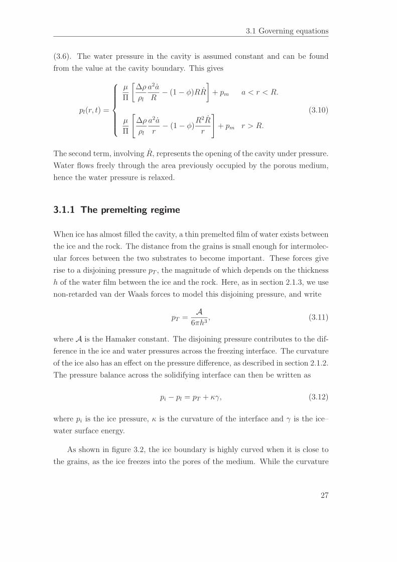
(3.6). The water pressure in the cavity is assumed constant and can be found
from the value at the cavity boundary. This gives
pl(r, t) =
µ
Π
[∆ρ
ρl
a2a
R− (1 − φ)RR
]
+ pm a < r < R.
µ
Π
[
∆ρ
ρl
a2a
r− (1 − φ)
R2R
r
]
+ pm r > R.
(3.10)
The second term, involving R, represents the opening of the cavity under pressure.
Water flows freely through the area previously occupied by the porous medium,
hence the water pressure is relaxed.
3.1.1 The premelting regime
When ice has almost filled the cavity, a thin premelted film of water exists between
the ice and the rock. The distance from the grains is small enough for intermolec-
ular forces between the two substrates to become important. These forces give
rise to a disjoining pressure pT , the magnitude of which depends on the thickness
h of the water film between the ice and the rock. Here, as in section 2.1.3, we use
non-retarded van der Waals forces to model this disjoining pressure, and write
pT =A
6πh3, (3.11)
where A is the Hamaker constant. The disjoining pressure contributes to the dif-
ference in the ice and water pressures across the freezing interface. The curvature
of the ice also has an effect on the pressure difference, as described in section 2.1.2.
The pressure balance across the solidifying interface can then be written as
pi − pl = pT + κγ, (3.12)
where pi is the ice pressure, κ is the curvature of the interface and γ is the ice–
water surface energy.
As shown in figure 3.2, the ice boundary is highly curved when it is close to
the grains, as the ice freezes into the pores of the medium. While the curvature
27
3 The spherical cavity
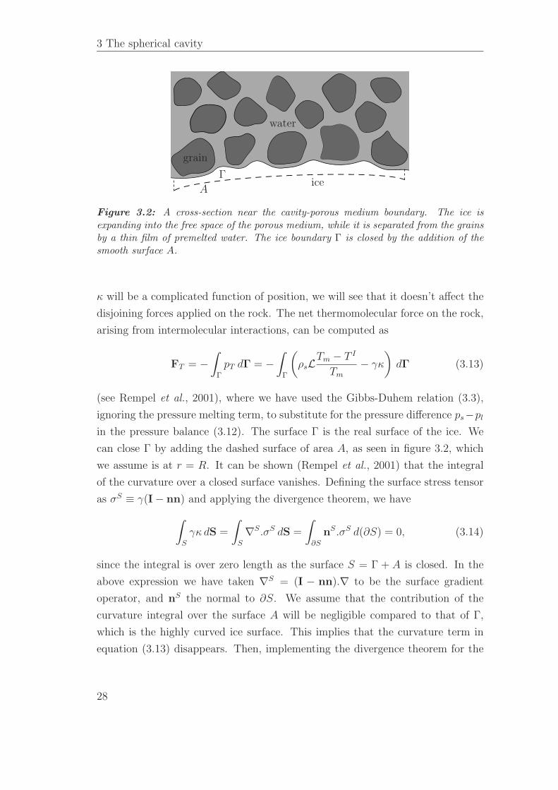
grain
water
iceΓ
A
Figure 3.2: A cross-section near the cavity-porous medium boundary. The ice isexpanding into the free space of the porous medium, while it is separated from the grainsby a thin film of premelted water. The ice boundary Γ is closed by the addition of thesmooth surface A.
κ will be a complicated function of position, we will see that it doesn’t affect the
disjoining forces applied on the rock. The net thermomolecular force on the rock,
arising from intermolecular interactions, can be computed as
FT = −∫
Γ
pT dΓ = −∫
Γ
(
ρsLTm − T I
Tm
− γκ
)
dΓ (3.13)
(see Rempel et al., 2001), where we have used the Gibbs-Duhem relation (3.3),
ignoring the pressure melting term, to substitute for the pressure difference ps−pl
in the pressure balance (3.12). The surface Γ is the real surface of the ice. We
can close Γ by adding the dashed surface of area A, as seen in figure 3.2, which
we assume is at r = R. It can be shown (Rempel et al., 2001) that the integral
of the curvature over a closed surface vanishes. Defining the surface stress tensor
as σS ≡ γ(I − nn) and applying the divergence theorem, we have
∫
S
γκ dS =
∫
S
∇S.σS dS =
∫
∂S
nS.σS d(∂S) = 0, (3.14)
since the integral is over zero length as the surface S = Γ + A is closed. In the
above expression we have taken ∇S = (I − nn).∇ to be the surface gradient
operator, and nS the normal to ∂S. We assume that the contribution of the
curvature integral over the surface A will be negligible compared to that of Γ,
which is the highly curved ice surface. This implies that the curvature term in
equation (3.13) disappears. Then, implementing the divergence theorem for the
28
3.1 Governing equations
remaining term, we find
FT = −ρsLTm
∫
V
∇(Tm − T I) dV +ρsLTm
∫
A
(Tm − T I) dA. (3.15)
Since the temperature in the ice is constant, the first term on the RHS vanishes,
while the second one simply gives
FT = ρsLATm − T I
Tm
r. (3.16)
The important conclusion here is that the net thermomolecular force is indepen-
dent of the curvature and independent of the type and strength of interactions
that give rise to the disjoining pressure pT (see Rempel et al., 2001). Moreover,
it depends only on the approximated boundary A and not on the microscopically
complicated surface Γ, hence we are justified to treat the ice–water–rock bound-
ary as macroscopically smooth. We will ignore the curvature term in the pressure
balance across the freezing front from now on and the effect of the curvature on
the pressure applied on the rock will be discussed in section 3.2.1.
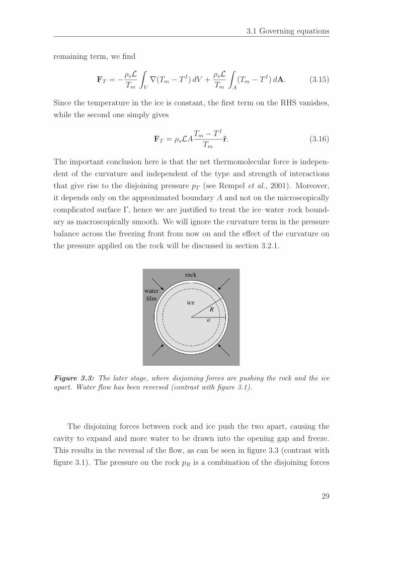
Figure 3.3: The later stage, where disjoining forces are pushing the rock and the iceapart. Water flow has been reversed (contrast with figure 3.1).
The disjoining forces between rock and ice push the two apart, causing the
cavity to expand and more water to be drawn into the opening gap and freeze.
This results in the reversal of the flow, as can be seen in figure 3.3 (contrast with
figure 3.1). The pressure on the rock pR is a combination of the disjoining forces
29
3 The spherical cavity
and the liquid pressure in the thin premelted film and hence is given by
pR − pl = pT . (3.17)
Since we are ignoring the curvature of the ice, the balance of pressures across the
premelted film becomes
pR = pi ≡ ps = pl + pT , (3.18)
i.e. the ice pressure pi and the rock pressure pR are equal.
To model the deformation of the cavity under pressure we use isotropic linear
elasticity with spherical symmetry which gives
ps(R, t) = 4G
(R
R0
− 1
)
, (3.19)
where R0 is the initial radius of the cavity and G is the shear modulus of the
material. The cavity starts expanding under the pressure that the growing ice
is exerting on its boundary. As the gap opens up, the disjoining pressure is
relaxed. More water flows towards the solidification front and freezes, increasing
the pressure applied on the cavity. Ultimately, the system reaches an equilibrium
where the disjoining pressure is balanced by the restoring force exerted by the
deformed rock.
While the analysis of the pressure balance has been done for the late-time
scenario, when the gap between the ice and the rock is very small, the pressure
balance described by equation (3.18) holds throughout the solidification process.
When the gap is large enough for disjoining forces to be negligible, i.e. pT ≈ 0, the
only pressure applied on the rock is the pressure of the liquid, i.e. pR = pl. Across
the freezing boundary we also have pi = pl, as we have ignored the effect of the
curvature of the boundary. Therefore, the balance of pressures can be described
by equation (3.18) at all times.
3.1.2 The dimensionless problem
We scale lengths with the initial cavity radius R0 and temperatures with the un-
dercooling temperature ∆T = Tm−T∞. We also take temperatures and pressures
30
3.1 Governing equations
to be relative to the corresponding values at infinity so that the scaled values van-
ish at r → ∞. A scale for velocities comes from the rate of solidification from
equation (3.4),
u0 =kl∆T
ρsLR0
. (3.20)
A time scale can be written as t0 = R0/u0 = ρsLR2/kl∆T . The pressure scale
comes from the left-hand side of the Gibbs-Thompson equation (2.8),
p∗ =ρsL∆T
Tm
(3.21)
and describes the pressure difference across an interface that causes depression
of the freezing temperature by ∆T . We denote the scaled ice radius by x(t) =
a(t)/R0 while, to keep notation simple, we use the same symbols for the scaled
versions of each variable. We can now also non-dimensionalize the flow velocity
u(r, t) =
ǫx2x
r2x < r < R
ǫx2x
r2− (1 − φ)
R2R
r2r > R
(3.22)
and the liquid pressure
pl(r, t) =
x2x
ǫΠR− 1 − φ
ǫ2ΠRR x < r < R,
x2x
ǫΠr− 1 − φ
ǫ2Π
R2R
rr > R,
(3.23)
where ǫ = ∆ρ/ρl and Π is the dimensionless parameter
Π =ρ2
sL2Π
µklǫ2Tm
, (3.24)
which can be thought of as a dimensionless permeability. Values for parameters
relating to water and ice can be found in table 3.1. The dimensionless heat balance
equation is simply given by
x(t)x(t) = T I(t), (3.25)
31
3 The spherical cavity
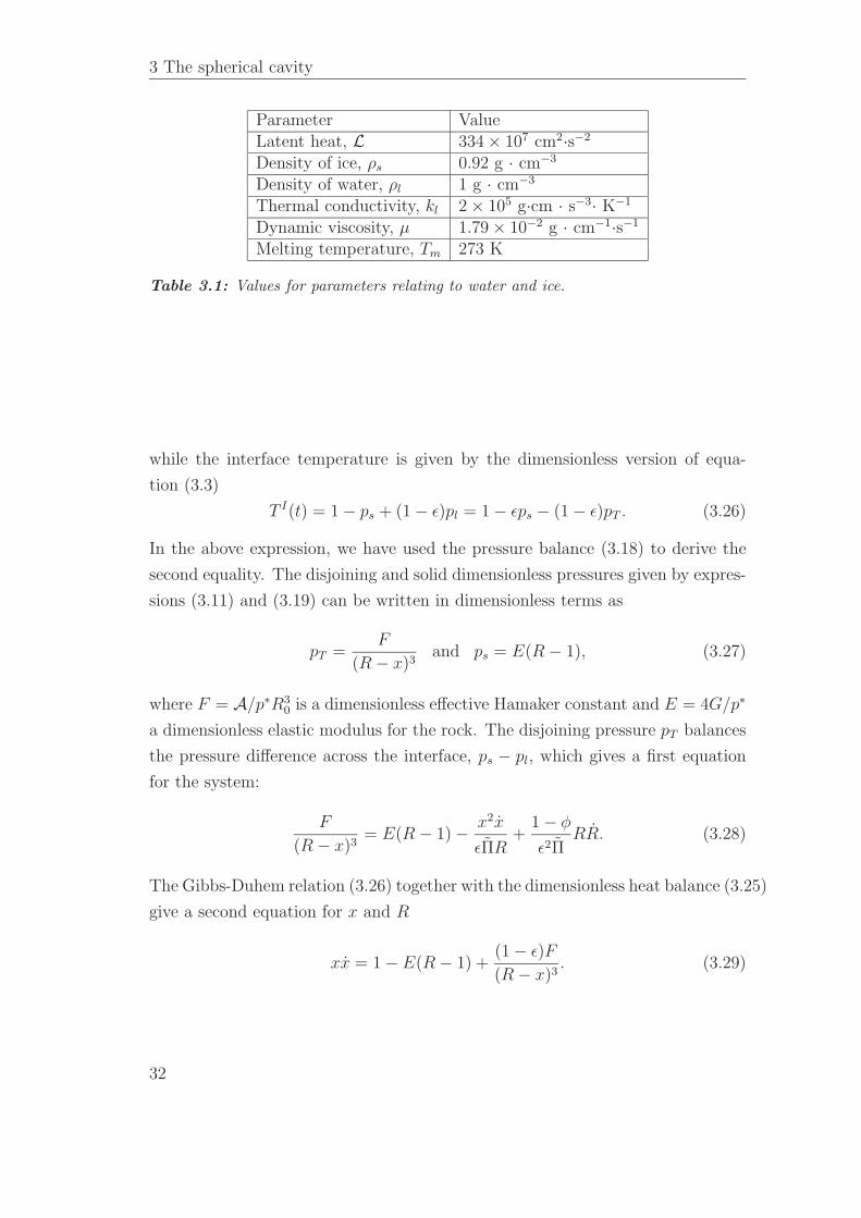
Parameter ValueLatent heat, L 334 × 107 cm2·s−2
Density of ice, ρs 0.92 g · cm−3
Density of water, ρl 1 g · cm−3
Thermal conductivity, kl 2 × 10⁵ g·cm · s−3· K−1
Dynamic viscosity, µ 1.79 × 10⁻² g · cm−1·s−1
Melting temperature, Tm 273 K
Table 3.1: Values for parameters relating to water and ice.
while the interface temperature is given by the dimensionless version of equa-
tion (3.3)
T I(t) = 1 − ps + (1 − ǫ)pl = 1 − ǫps − (1 − ǫ)pT . (3.26)
In the above expression, we have used the pressure balance (3.18) to derive the
second equality. The disjoining and solid dimensionless pressures given by expres-
sions (3.11) and (3.19) can be written in dimensionless terms as
pT =F
(R − x)3and ps = E(R − 1), (3.27)
where F = A/p∗R30 is a dimensionless effective Hamaker constant and E = 4G/p∗
a dimensionless elastic modulus for the rock. The disjoining pressure pT balances
the pressure difference across the interface, ps − pl, which gives a first equation
for the system:
F
(R − x)3= E(R − 1) − x2x
ǫΠR+
1 − φ
ǫ2ΠRR. (3.28)
The Gibbs-Duhem relation (3.26) together with the dimensionless heat balance (3.25)
give a second equation for x and R
xx = 1 − E(R − 1) +(1 − ǫ)F
(R − x)3. (3.29)
32
3.2 The expansion regime
3.2 The expansion regime
The initial stage of the process is the expansion stage, during which the solid ice
is still small compared to the cavity size so there is no interaction between the ice
and rock. While equations (3.28) and (3.29) will need to be solved numerically
to describe the full problem, we can use some approximations to derive some
important conclusions about this early regime analytically.
During the expansion stage, the disjoining forces are negligible, since the gap
R − x is large. Hence, we can ignore the F/(R − x)3 term on the left-hand-
side of equation (3.28) and the right-hand-side of equation (3.29). Then, we can
eliminate the E(R − 1) term between the two equations to find
xx +x2x
ΠR− 1 − φ
ǫΠRR = 1. (3.30)
The first term on the left-hand-side of equation (3.30) comes from the heat
balance and represents the flow of latent heat away from the solidification front,
while the second and third terms represent the pressure melting effect. They all
affect the rate of solidification: the transport of latent heat away from the freezing
front is necessary for the solidification to continue while a high pressure applied
on the ice will cause depression of the freezing temperature and hence the process
to slow down. The third term in particular expresses the relaxation in the liquid
pressure which is caused by the opening of the cavity. For stiff materials like
rocks, we expect the growth of the ice to be much faster than that of the rock, at
least during the early stages of freezing when the ice is not close enough to the
rock for the disjoining forces to be important, hence we can ignore the R term
and take R ≈ 1 for the rest of this section.
The first two terms are comparable when x ∼ ΠR ∼ 1015 × Π cm−2. Typical
permeability values vary from 10−3 cm2 for very permeable media such as highly
fractured rocks to 10−12 cm2- 10−15 cm2 for rocks like limestone, granite etc. Even
for very impermeable rocks (e.g. granite), the radius of the ice needs to be of the
order of the radius of the cavity for the two contributions to be comparable, so the
33
3 The spherical cavity
pressure melting term is only important for large ice radii and small permeabilities.
If we ignore the x2x term, we end up with
xx = 1 ⇒ x2 − x20 = 2t. (3.31)
Hence, in most cases the solidification happens without experiencing an effect
from the porous medium, and the ice grows proportional to t1/2.
The pressure in the cavity during the expansion regime can be written as
pexpansion =x
ǫ(1 + Π)≈ 11x
1 + 1.4 × Π × 1015cm−2, (3.32)
combining equation (3.23) with (3.30) and ignoring the R term. When x ≈ R
we enter a regime not covered by the approximations made in this section. If we
consider x large but not large enough for disjoining forces to become important,
we can have dimensional pressures varying from around 10−4p∗ (e.g. in sandstone)
to around 10p∗ in granite. How large is p∗? For an undercooling of ∆T = 1◦ K
we have
p∗ =ρsL∆T
Tm
≈ 11 atm, (3.33)
where we have taken the far-field pressure to be pm = 1 atm. Hence, the additional
pressure in the cavity varies from 10−3 atmospheres, which is negligible, to 102
atmospheres which is more than sufficient to fracture a rock. This shows us
that the expansion effect is very much dependent on the permeability of the
medium. For a water-saturated granite for example, the flow of water away from
the solidification front during the expansion stage can raise the pressure inside
the cavity significantly.
3.2.1 Curvature effect and critical nucleation radius
We can include the effect of curvature on the freezing temperature in the Gibbs-
Duhem equation (3.26) which becomes
T I = 1 − Γ
x− x2x
Π, (3.34)
34
3.2 The expansion regime
where we have defined a dimensionless surface tension
Γ =2γTm
ρsLR0∆T. (3.35)
Combining this with the heat balance (3.25) we find
xx = 1 − Γ
x− x2x
Π⇒ x =
Π(x − Γ)
x2(x + Π). (3.36)
The expression for the pressure in the cavity will also change in a similar way
pexp =x − Γ
ǫ(x + Π). (3.37)
The surface tension for the water–ice interface is γ ≈ 33 erg/cm2 so Γ = O(10−5)
when R0 = 1 cm and ∆T = 1 K. As before, the maximum pressure in the cavity
occurs when x = O(1). Since Γ ≪ 1, the effect of curvature melting is negligible
and the extra term can be ignored.
Equation (3.36) also shows that growth only occurs if x > Γ, i.e. there
is a minimum radius of the ice nucleus, below which no ice growth occurs. In
dimensional terms this condition becomes
a > amin ≡ 2γTm
ρsL∆T. (3.38)
The critical nucleation radius is independent of the permeability of the rock and
the radius of the cavity hence it solely depends on the curvature of the sphere.
The permeability of the porous medium doesn’t determine whether ice nucleation
is possible apart from in the special case Π = 0, i.e. when the rock is impermeable,
where no ice can grow. This is a result of the volume increase occurring during
solidification, owing to the density difference of ice and water, resulting in flow
away from the solidification front. Since no water can flow through the porous
medium when Π = 0, no freezing can occur.
35
3 The spherical cavity
3.3 Full results
We solve the full problem, governed by the system of differential equations (3.28)
and (3.29) using Matlab’s solver ode15s. This solver is chosen as it is suitable for
stiff problems like the one here. Since the disjoining pressure term F/(R − x)3
is acting only in a small region of the problem, there are two different scales
and the required step to capture that behaviour is very small. A non-stiff solver
would require a lot more steps to produce accurate results. For the following
examples, we use a value of the Hamaker constant A a few orders of magnitude
larger than the real one, as it helps makes the graphs clearer (a larger A means
that the gap between ice and rock h is larger) and saves computational time.
Smaller values of A require much smaller steps but do not alter the qualitative
results. Typical values of the shear modulus are G ≈ 10 − 100 GPa for rocks like
limestone or granite (see also section 7.2). This corresponds to a dimensionless
elastic modulus of E ≈ 9−90 ·103. In the examples presented here, we have used
a slightly smaller value of E = 3000 to make the deformation of the cavity more
visible, but the qualitative conclusions remain the same.
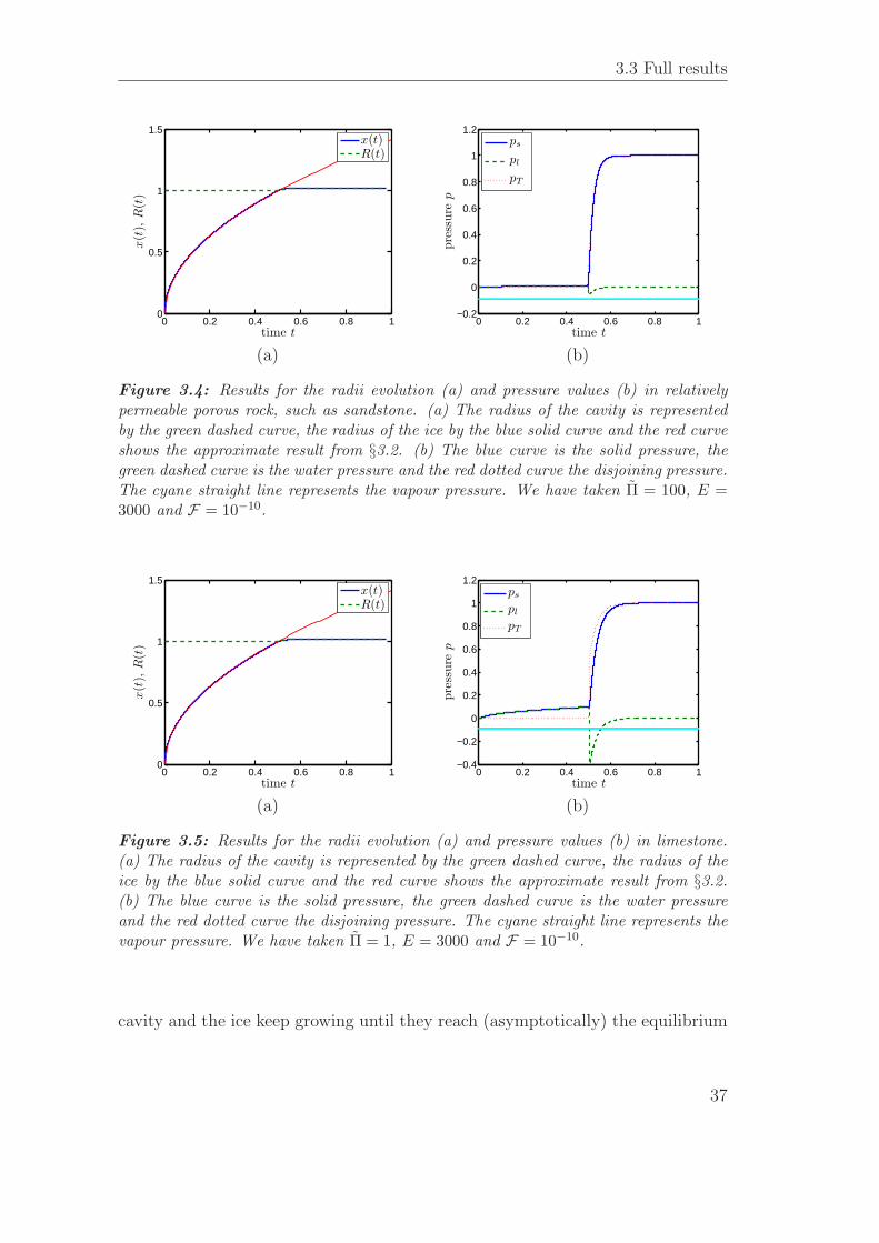
Graphs 3.4-3.6 show results for the evolution of the radius of the ice and the
cavity (left), and the liquid and solid pressures (right) plotted against time for
three different types of rock. The first one, graph 3.4 shows results for a sandstone
with permeability of 10−12 cm2. There are three distinct regions. The first one
extends up to about t = 0.45 and describes the expansion regime. We notice that
the expansion of the cavity itself is negligible, while the evolution of the solid
ice agrees very well with the t1/2 behaviour (red line) predicted in the expansion
section. There is no pressure difference across the solidification front since we are
ignoring curvature effects and the disjoining forces are negligible (red dotted line).
The important thing to note is that the maximum pressure during the expansion
regime is much smaller than the maximum disjoining pressure. The second region
is characterized by a very fast increase in the disjoining forces. The ice is now
close enough to the cavity for intermolecular forces to become important and the
solidification process has slowed down considerably since the ice is limited by
the cavity boundary. Disjoining forces cause the cavity to expand and water to
be sucked into the gap as we can see from the drop in the water pressure, which
becomes negative. The third and last region is the recovery phase, where both the
36
3.3 Full results
0 0.2 0.4 0.6 0.8 10
0.5
1
1.5
time t
x(t
),R
(t)
x(t)R(t)
0 0.2 0.4 0.6 0.8 1−0.2
0
0.2
0.4
0.6
0.8
1
1.2
time t
pre
ssure
p
ps
pl
pT
(a) (b)
Figure 3.4: Results for the radii evolution (a) and pressure values (b) in relativelypermeable porous rock, such as sandstone. (a) The radius of the cavity is representedby the green dashed curve, the radius of the ice by the blue solid curve and the red curveshows the approximate result from §3.2. (b) The blue curve is the solid pressure, thegreen dashed curve is the water pressure and the red dotted curve the disjoining pressure.The cyane straight line represents the vapour pressure. We have taken Π = 100, E =3000 and F = 10−10.
0 0.2 0.4 0.6 0.8 10
0.5
1
1.5
time t
x(t
),R
(t)
x(t)R(t)
0 0.2 0.4 0.6 0.8 1−0.4
−0.2
0
0.2
0.4
0.6
0.8
1
1.2
time t
pre
ssure
p
ps
pl
pT
(a) (b)
Figure 3.5: Results for the radii evolution (a) and pressure values (b) in limestone.(a) The radius of the cavity is represented by the green dashed curve, the radius of theice by the blue solid curve and the red curve shows the approximate result from §3.2.(b) The blue curve is the solid pressure, the green dashed curve is the water pressureand the red dotted curve the disjoining pressure. The cyane straight line represents thevapour pressure. We have taken Π = 1, E = 3000 and F = 10−10.
cavity and the ice keep growing until they reach (asymptotically) the equilibrium
37
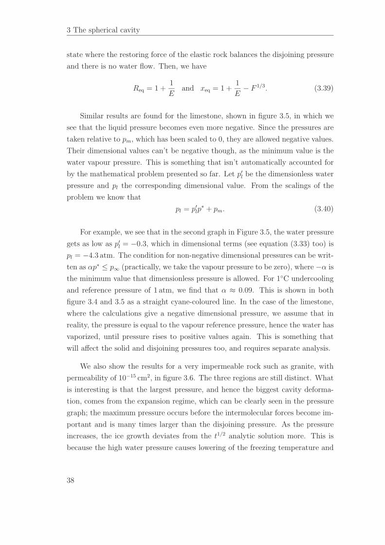
3 The spherical cavity
state where the restoring force of the elastic rock balances the disjoining pressure
and there is no water flow. Then, we have
Req = 1 +1
Eand xeq = 1 +
1
E− F 1/3. (3.39)
Similar results are found for the limestone, shown in figure 3.5, in which we
see that the liquid pressure becomes even more negative. Since the pressures are
taken relative to pm, which has been scaled to 0, they are allowed negative values.
Their dimensional values can’t be negative though, as the minimum value is the
water vapour pressure. This is something that isn’t automatically accounted for
by the mathematical problem presented so far. Let p′l be the dimensionless water
pressure and pl the corresponding dimensional value. From the scalings of the
problem we know that
pl = p′lp∗ + pm. (3.40)
For example, we see that in the second graph in Figure 3.5, the water pressure
gets as low as p′l = −0.3, which in dimensional terms (see equation (3.33) too) is
pl = −4.3 atm. The condition for non-negative dimensional pressures can be writ-
ten as αp∗ ≤ p∞ (practically, we take the vapour pressure to be zero), where −α is
the minimum value that dimensionless pressure is allowed. For 1◦C undercooling
and reference pressure of 1 atm, we find that α ≈ 0.09. This is shown in both
figure 3.4 and 3.5 as a straight cyane-coloured line. In the case of the limestone,
where the calculations give a negative dimensional pressure, we assume that in
reality, the pressure is equal to the vapour reference pressure, hence the water has
vaporized, until pressure rises to positive values again. This is something that
will affect the solid and disjoining pressures too, and requires separate analysis.
We also show the results for a very impermeable rock such as granite, with
permeability of 10−15 cm2, in figure 3.6. The three regions are still distinct. What
is interesting is that the largest pressure, and hence the biggest cavity deforma-
tion, comes from the expansion regime, which can be clearly seen in the pressure
graph; the maximum pressure occurs before the intermolecular forces become im-
portant and is many times larger than the disjoining pressure. As the pressure
increases, the ice growth deviates from the t1/2 analytic solution more. This is
because the high water pressure causes lowering of the freezing temperature and
38
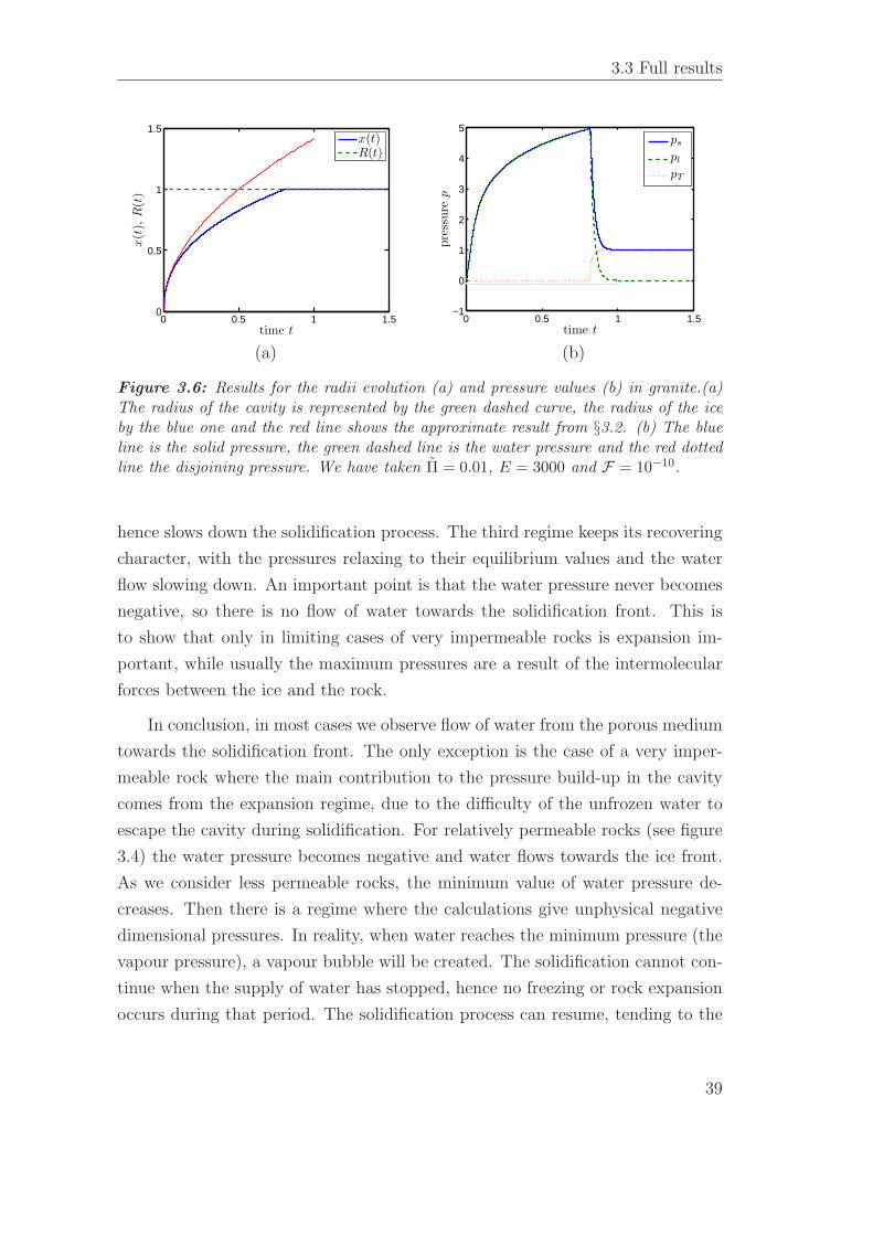
3.3 Full results
0 0.5 1 1.50
0.5
1
1.5
time t
x(t
),R
(t)
x(t)R(t)
0 0.5 1 1.5−1
0
1
2
3
4
5
time t
pre
ssure
p
ps
pl
pT
(a) (b)
Figure 3.6: Results for the radii evolution (a) and pressure values (b) in granite.(a)The radius of the cavity is represented by the green dashed curve, the radius of the iceby the blue one and the red line shows the approximate result from §3.2. (b) The blueline is the solid pressure, the green dashed line is the water pressure and the red dottedline the disjoining pressure. We have taken Π = 0.01, E = 3000 and F = 10−10.
hence slows down the solidification process. The third regime keeps its recovering
character, with the pressures relaxing to their equilibrium values and the water
flow slowing down. An important point is that the water pressure never becomes
negative, so there is no flow of water towards the solidification front. This is
to show that only in limiting cases of very impermeable rocks is expansion im-
portant, while usually the maximum pressures are a result of the intermolecular
forces between the ice and the rock.
In conclusion, in most cases we observe flow of water from the porous medium
towards the solidification front. The only exception is the case of a very imper-
meable rock where the main contribution to the pressure build-up in the cavity
comes from the expansion regime, due to the difficulty of the unfrozen water to
escape the cavity during solidification. For relatively permeable rocks (see figure
3.4) the water pressure becomes negative and water flows towards the ice front.
As we consider less permeable rocks, the minimum value of water pressure de-
creases. Then there is a regime where the calculations give unphysical negative
dimensional pressures. In reality, when water reaches the minimum pressure (the
vapour pressure), a vapour bubble will be created. The solidification cannot con-
tinue when the supply of water has stopped, hence no freezing or rock expansion
occurs during that period. The solidification process can resume, tending to the
39
3 The spherical cavity
steady state shown in the third regime, when water from the medium has reached
the freezing front. The timescale of this process will depend on the permeabil-
ity of the medium as less permeable rocks limit the flow of water more. This
regime requires a different approach, as the assumption of the ice–water–rock in-
terface, and the subsequent pressure balance, break down. Further analysis of
this phenomenon is beyond the scope of this thesis.
3.4 Conclusions
We have studied the process of water freezing inside a spherical cavity and how
the growth of ice can create high pressures inside the cavity. We have identified
the main features of the process: the expansion of the water when it freezes and
the disjoining forces across a thin premelted film that develop when the ice has
grown to be close enough to the rock. We have compared the effect that those
two processes have on the pressure inside the cavity and how they depend on
the permeability of the rock. This has shown that it is only in the case of very
impermeable rocks, like granite, that expansion can raise the pressure enough to
cause a fracture. For more permeable rocks, the water can escape the cavity easily
during solidification without experiencing any influence of the porous medium.
Therefore, the main rise in pressure comes from the premelting stage when the
ice is very close to the rock. In this case the flow reverses and the water flows
towards the solidification front. This is a result of disjoining forces that push the
ice and the rock apart and cause the water pressure to drop. These disjoining
forces can easily reach several atmospheres even for very small undercoolings,
which indicates that they could be responsible for the fracturing of rocks.
Although the work presented here is done for a simple geometry, it provides
insight into the processes that take place during the freezing of water-saturated
rocks. It demonstrates the relative importance of expansion and premelting and
shows that, in most cases, high pressures occur at the later stage where the ice has
extended to the cavity boundary, therefore justifying our focusing future attention
to ice-filled cavities. The idealized model developed here provides us with some
important conclusions about the importance of the different interactions taking
place inside the cavity. These conclusions can work as a basis for a mathematical
analysis of more complicated and realistic geometries.
40
Chapter 4
The penny-shaped crack
We have so far studied ice growth inside a spherical cavity and the pressure
build-up associated with the different processes taking place. We now have an
understanding of the different balances between these processes which will be
useful in our study of more complicated problems.
In order to develop a more realistic model of frost fracturing, we will have to
look at more relevant geometries. Ice growth inside pre-existing faults in rocks,
and the large pressures associated with it, will cause asymmetric growth of the
faults, with the resulting crack likely to have two dimensions much larger than
the third. Penny-shaped cracks were considered by Walder & Hallet (1985), who
simply assumed a uniform pressure within each crack, resulting in elliptical profiles
(see section 4.2.1). Complications arise if we attempt to account for curvature-
induced melting of the ice, which can be an important effect, especially close to
41

4 The penny-shaped crack
the tip of the crack. We will attempt to address these points and consider the
geometry of an isolated crack in more detail. Our aim is to develop a mathematical
model combining fluid dynamics, thermodynamics and elasticity theory that will
allow us to describe the processes taking place inside an ice-filled crack in order
to make predictions of its shape and evolution.
In this chapter, we will develop the equations describing the fluid dynamics
and linear elasticity of the problem, study some simple scalings that arise from the
coupling of the two solid and liquid pressure fields and discuss numerical methods
that can be used to tackle the problem further. We will focus on the balance of
pressures and solve the problem for the propagation of a cavity under uniform
pressure and only restricted by the water supply at the freezing front. We will
find that the propagation rate cannot be determined by fluid dynamic arguments
alone, and the dynamics of the crack need to be studied further. Despite this,
many interesting features arise from the analytic solution obtained, and it is also
used as a test for the two numerical methods developed.
4.1 Setting the problem
In an attempt to model this more complicated geometry, we will consider an ax-
isymmetric, penny-shaped crack of radius R(t) and small width b(r, t) ≪ R(t).
The crack is considered to be inside an elastic porous rock that is large enough
compared to the crack to be treated as infinite in extent. The rock is satu-
rated with water that has been supercooled to a uniform temperature T∞ < Tm,
where Tm is the melting temperature of the ice measured at the reference pres-
sure pm = p∞. In this section, we assume that the crack and the rock remain
isothermal. The latent heat produced during solidification has to be transported
away from the freezing front in order for the process to continue. This requires
a temperature gradient normal to the surface, and the transfer of energy is de-
scribed mathematically by the Stefan condition (2.15). As we saw in section
3.1.1, when the solidification rate is dominated by the latent heat transfer, the
growth of the ice behaves like t1/2. This behaviour is seen in figures 3.4-3.6 for
early times but, as soon as the ice is close enough to the cavity boundary for the
disjoining pressure pT to become important, the growth slows down dramatically.
42
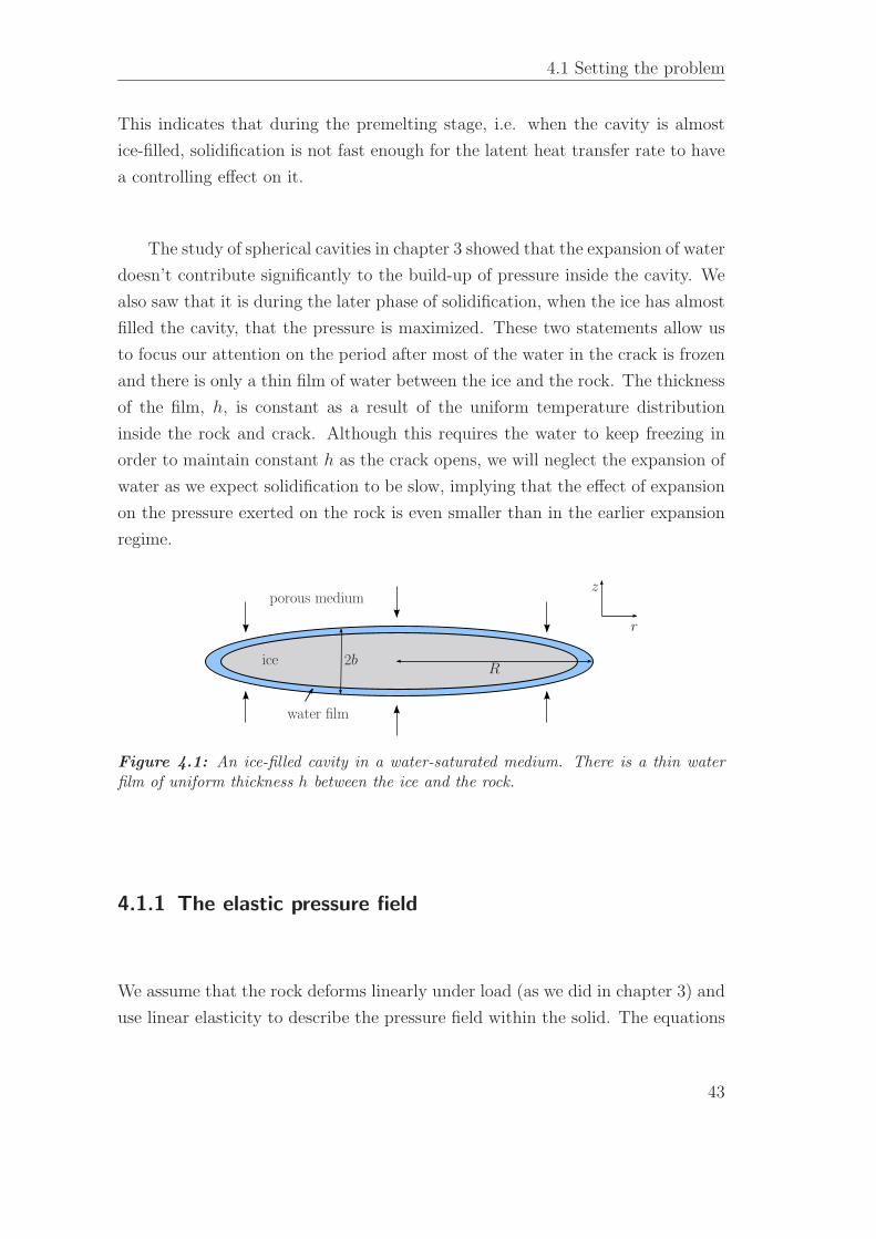
4.1 Setting the problem
This indicates that during the premelting stage, i.e. when the cavity is almost
ice-filled, solidification is not fast enough for the latent heat transfer rate to have
a controlling effect on it.
The study of spherical cavities in chapter 3 showed that the expansion of water
doesn’t contribute significantly to the build-up of pressure inside the cavity. We
also saw that it is during the later phase of solidification, when the ice has almost
filled the cavity, that the pressure is maximized. These two statements allow us
to focus our attention on the period after most of the water in the crack is frozen
and there is only a thin film of water between the ice and the rock. The thickness
of the film, h, is constant as a result of the uniform temperature distribution
inside the rock and crack. Although this requires the water to keep freezing in
order to maintain constant h as the crack opens, we will neglect the expansion of
water as we expect solidification to be slow, implying that the effect of expansion
on the pressure exerted on the rock is even smaller than in the earlier expansion
regime.
porous medium
ice
water film
2b
z
r
R
Figure 4.1: An ice-filled cavity in a water-saturated medium. There is a thin waterfilm of uniform thickness h between the ice and the rock.
4.1.1 The elastic pressure field
We assume that the rock deforms linearly under load (as we did in chapter 3) and
use linear elasticity to describe the pressure field within the solid. The equations
43
4 The penny-shaped crack
relating stress to displacement in cylindrical coordinates are (Sneddon, 1951)
σrr = (λ + 2G)∂ur
∂r+ λ
ur
r+ λ
∂uz
∂z, (4.1)
σθθ = λ∂ur
∂r+ (λ + 2G)
ur
r+ λ
∂uz
∂z, (4.2)
σzz = λ∂ur
∂r+ λ
ur
r+ (λ + 2G)
∂uz
∂z, (4.3)
σrz = G
(∂ur
∂z+
∂uz
∂r
)
, (4.4)
where the subscripts represent components of the stress tensor σ and the displace-
ment vector u. The constant λ is Lame’s first parameter while G is the shear
modulus. Solving the equations above can be reduced to solving the biharmonic
equation (see Appendix A.1)
∇4Φ = 0, (4.5)
where the function Φ is related to the stress field by
ur =λ + G
GΦrz, (4.6)
uz =λ + 2G
G∇2Φ − λ + G
GΦzz. (4.7)
There are several methods that can be used to find solutions for the pres-
sure and displacement field using the function Φ. Different approaches are suited
to different problems and their simplicity depends on the geometry of the prob-
lem and the boundary conditions. For the configuration here, we follow Spence
& Sharp (1985) and assume that the crack has zero internal shear stress, i.e.
σrz(r, 0) = 0. By symmetry, the problem for the disk-shaped cavity is equivalent
to that for a half space z > 0 with prescribed pressure field within the circle r < R
and no normal displacement for r > R. Then, the expressions for the pressure
p(r, z) and the displacement b(r) become (Sneddon, 1951, and see Appendix A.2)
p(r, z) = −σzz(r, z) = 2(λ + G)
∫∞
0
ξ3e−ξzB(ξ)(1 + ξz)J0(rξ) dξ, (4.8)
b(r) = uz(r, 0) = −λ + 2G
G
∫∞
0
ξ2B(ξ)J0(rξ) dξ. (4.9)
44
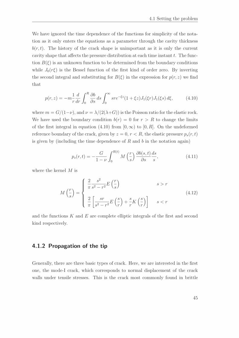
4.1 Setting the problem
We have ignored the time dependence of the functions for simplicity of the nota-
tion as it only enters the equations as a parameter through the cavity thickness
b(r, t). The history of the crack shape is unimportant as it is only the current
cavity shape that affects the pressure distribution at each time instant t. The func-
tion B(ξ) is an unknown function to be determined from the boundary conditions
while J0(rξ) is the Bessel function of the first kind of order zero. By inverting
the second integral and substituting for B(ξ) in the expression for p(r, z) we find
that
p(r, z) = −m1
r
d
dr
∫ R
0
∂b
∂sds
∫∞
0
sre−ξz(1 + ξz)J1(ξr)J1(ξs) dξ, (4.10)
where m = G/(1−ν), and ν = λ/(2(λ+G)) is the Poisson ratio for the elastic rock.
We have used the boundary condition b(r) = 0 for r > R to change the limits
of the first integral in equation (4.10) from [0,∞) to [0, R]. On the undeformed
reference boundary of the crack, given by z = 0, r < R, the elastic pressure ps(r, t)
is given by (including the time dependence of R and b in the notation again)
ps(r, t) = − G
1 − ν
∫ R(t)
0
M(r
s
) ∂b(s, t)
∂s
ds
s, (4.11)
where the kernel M is
M(r
s
)
=
2
π
s2
s2 − r2E
(r
s
)
s > r
2
π
[sr
s2 − r2E
(s
r
)
+s
rK
(s
r
)]
s < r
(4.12)
and the functions K and E are complete elliptic integrals of the first and second
kind respectively.
4.1.2 Propagation of the tip
Generally, there are three basic types of crack. Here, we are interested in the first
one, the mode-I crack, which corresponds to normal displacement of the crack
walls under tensile stresses. This is the crack most commonly found in brittle
45
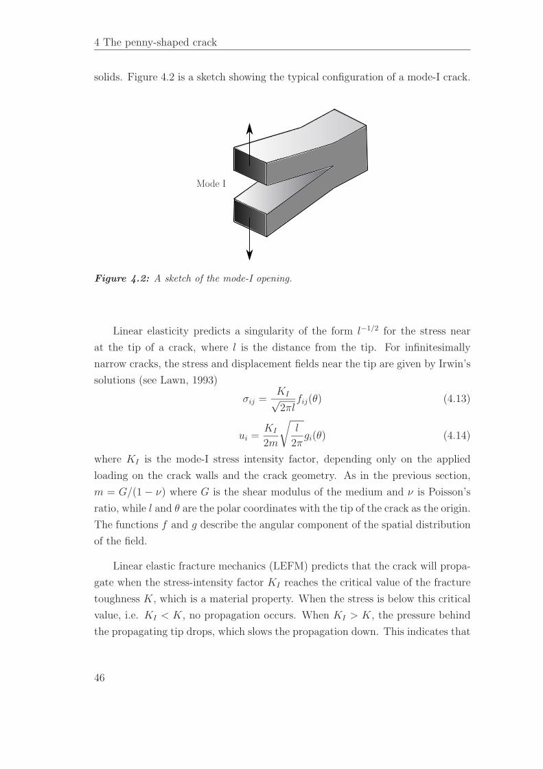
4 The penny-shaped crack
solids. Figure 4.2 is a sketch showing the typical configuration of a mode-I crack.
Mode I
Figure 4.2: A sketch of the mode-I opening.
Linear elasticity predicts a singularity of the form l−1/2 for the stress near
at the tip of a crack, where l is the distance from the tip. For infinitesimally
narrow cracks, the stress and displacement fields near the tip are given by Irwin’s
solutions (see Lawn, 1993)
σij =KI√2πl
fij(θ) (4.13)
ui =KI
2m
√
l
2πgi(θ) (4.14)
where KI is the mode-I stress intensity factor, depending only on the applied
loading on the crack walls and the crack geometry. As in the previous section,
m = G/(1 − ν) where G is the shear modulus of the medium and ν is Poisson’s
ratio, while l and θ are the polar coordinates with the tip of the crack as the origin.
The functions f and g describe the angular component of the spatial distribution
of the field.
Linear elastic fracture mechanics (LEFM) predicts that the crack will propa-
gate when the stress-intensity factor KI reaches the critical value of the fracture
toughness K, which is a material property. When the stress is below this critical
value, i.e. KI < K, no propagation occurs. When KI > K, the pressure behind
the propagating tip drops, which slows the propagation down. This indicates that
46
4.1 Setting the problem
propagation occurs in the marginal state KI = K. Using the Irwin equations, we
can show (Savitski & Detournay, 2002) that the near-field of the crack is parabolic
in shape
b ∼ K
m
[8(R − r)
π
]1/2
, as r → R. (4.15)
An alternative expression for the stress-intensity factor can be derived by consid-
ering the effect that a given loading at the inner walls of a crack has on the stress
at the tip (see Lawn, 1993, pg. 33). We assume that the load p(r) is axisymmet-
ric and continuously distributed along the inner walls. The stress-intensity factor
produced by this load is then given by
KI =2√πR
∫ R
0
rp(r)√R2 − r2
dr. (4.16)
When the crack is at the critical state KI = K, the last two expressions are
equivalent (see Rice, 1968).
4.1.3 The water pressure distribution
We now consider the pressure distribution of water inside the cavity and the
porous medium. The flow of water through the pores is described by Darcy’s
equation
µu = −Π∇p, (4.17)
where µ is the dynamic viscosity of water and Π the permeability of the medium.
We combine (4.17) with the mass continuity equation ∇.u = 0 to find that the
water pressure p satisfies Laplace’s equation ∇2p = 0 everywhere apart from
inside the crack. The pressure can hence be given in terms of a Green’s function:
p =µ
4πΠ
∫
disk
q(r′)
|x − r′| dr′ =µ
4πΠ
∫
disk
q(r′)r′ dr′ dθ′
(r2 + r′2 − 2rr′ cos θ′ + z2)1/2, (4.18)
where q(r) is the flux of water into the cavity
q(r) = −2Π
µlimz→0
∂p
∂z. (4.19)
47

4 The penny-shaped crack
The θ-integral can be expressed as an elliptic integral of the first type. We denote
the water pressure on the boundary z = b(r, t) as pl. The boundary condition can
be evaluated at z = 0 for simplicity, since the cavity opening b is small compared
to the length of the crack. Then,
pl(r, t) =µ
πΠ
∫ R
0
sq(s, t)
r + sK
(2√
rs
r + s
)
ds, (4.20)
where K is the complete elliptic integral of the first kind.
Inside the cavity, water flows in the film between the ice and the rock. As-
suming there is no flow in the θ direction, we write the velocities in the direction
of r and z as v and w respectively. Because h is small, we can use lubrication
theory to approximate the flow in the thin film. Since we are assuming a con-
stant thickness h, we are ignoring the time-dependence of the flow using steady
Navier-Stokes∂p
∂z= 0 and
∂p
∂r= µ
∂2v
∂z2, (4.21)
which give the solution
v =1
2µ
∂p
∂r(z − b)(z − b + h), (4.22)
satisfying the no-slip condition at the rock and ice boundaries.
ice
water
water
rockwater flow
r
z∂b
∂t
∂b
∂t h
−u
freezing
flow along thin film
Figure 4.3: A sketch of the premelted film, showing the different contributions to waterflow in and out of it.
Water flows inside the thin gap and freezes at the ice boundary. Since we
have assumed that the gap h is uniform, the rate of growth of the ice is the
48
4.1 Setting the problem
same as the rate of opening of the cavity, i.e. ∂b∂t
. We can use mass conservation
inside the thin film to deduce an equation for the rate of cavity opening ∂b∂t
.
The film changes as seen in figure 4.3, with the dashed curves representing the
film after time δt. The bottom of the boundary moves as the water occupying
b − h < z < b − h + δb freezes. Since we have ignored the expansion of water as
it freezes, this corresponds to a volume flux (per unit area) out of the gap of ∂b∂t
hence, at z = b−h, the velocity at the vertical direction is w = −∂b∂t
. Water flows
into the gap from the porous medium as described by the Darcy equation (4.17)
hence, at z = b, we have w = u. The mass continuity equation is
1
r
∂
∂r(rv) +
∂w
∂z= 0 (4.23)
which, integrated from z = b − h to z = b, gives an equation for the evolution of
the cavity width b(r, t)
∂b
∂t+
1
r
∂
∂r
(
rh3
12µ
∂pl
∂r
)
= −u(b) =Π
µ
∂p
∂z
∣∣∣z=b
, (4.24)
where the second equality comes from Darcy’s equation (4.17).
We estimate the sizes of the terms in the equation above, denoting the char-
acteristic length scale by L and the pressure scale by P . The lubrication flow term
on the left-hand side of equation (4.24) describes flow in the thin gap between
the ice and the rock while the pressure term on the right-hand side represents the
flow of water from the porous medium towards the solidification front. Using the
pressure and length scales we find the ratio of these two terms to be
h3
12µ
P
L2:Π
µ
P
L=
h3
12Π: L. (4.25)
The left-hand side of (4.25) is at most about 10−4 cm (since the thickness of
the film h is of the order of 10 nm, see also section 2.1.3), while the size of a
typical cavity will be several orders of magnitude larger. Hence, the flow through
the porous medium dominates over the flow in the thin films. This allows us to
ignore the lubrication flow term and to write equation (4.24) in the much simpler
form∂b
∂t=
Π
µ
∂p
∂z
∣∣∣z=b
≈ Π
µ
∂p
∂z
∣∣∣z=0
= −1
2q(r, t). (4.26)
49
4 The penny-shaped crack
The integral equation for pl (4.20) can now be written in terms of b(r, t)
pl(r, t) = − 2
π
µ
Π
∫ R(t)
0
K
(2√
rs
r + s
)∂b(s, t)
∂t
s ds
r + s. (4.27)
4.1.4 The pressure balance
We saw in chapter 2 that a difference in the solid–liquid pressure on a freezing
surface can be caused by several effects. The presence of a foreign substance close
to the boundary of the ice can cause a disjoining pressure acting across the film
of water. A curved surface also causes a difference in the pressures across the
freezing interface and depresses the freezing temperature. While studying the
spherical model we found that the effect of the curvature of the surface of the
spherical nucleus is unimportant (see section 3.2.1). Here, we are dealing with
even smaller curvatures since the surface of the penny-shaped ice is much flatter
than the spherical one. The only exception is at the tip of the crack, where the
curvature becomes very large. This could affect the extent of the ice into the tip
of the cavity, as we will discuss towards the end of section 4.2.1.
Close to the rock, we expect the ice to no longer be smooth but highly curved,
extending into the pores of the medium, as described by figure 3.2 (see section
3.1.1). At the beginning of section 3.1.1 we showed why this effect is negligible
and how we can treat the freezing front as a smooth surface, in a similar way to
Rempel et al. (2001). The solid–liquid pressure difference hence must simply be
balanced by the disjoining pressure
ps − pl = pT . (4.28)
The density difference between the solid and liquid phases is again ignored
here, as in section 4.1.3. Its effect on the freezing temperature occurs through
the phenomenon of pressure melting. A departure of the liquid pressure from the
reference value causes a change in the freezing temperature, as described by the
Gibbs-Duhem equation (2.8). In terms of ps and pl, the dimensionless interface
temperature is given by
T I = 1 − (ps − pl) + ǫpl(x, t), (4.29)
50
4.2 Similarity solution
where ǫ = ∆ρ/ρl and the second term on the right-hand-side describes the
pressure-melting effect. The pl terms can be combined to give (1 − ǫ)pl and,
since the ǫ ≈ 0.1, we can approximate it as (1 − ǫ)pl ≈ pl, i.e. taking ǫ ≈ 0. The
interface undercooling (in dimensional terms) is therefore simply given by
ρsL∆T
Tm
= ps − pl. (4.30)
4.2 Similarity solution
We begin by investigating a crack whose propagation is limited only by the ability
of water to flow through the porous rock and feed the growing ice, rather than
determined by considerations of the material fracture toughness.
In addition to the length and pressure scales L and P we define the time scale
t∗. The balance of terms in the pressure balance equation (4.28) gives
m ∼ µ
Π
L2
t∗⇒ L ∼
(Πm
µt∗
)1/2
. (4.31)
There is no other constraint on the time scale so t∗ simply is the elapsed time t.
The radius of the cavity then propagates according to
R(t) = k
(Πm
µt
)1/2
, (4.32)
where k is a constant of proportionality that has to be determined. Since the
cavity shape scales with the elapsed time and there is no inherent time scale in
the problem we can find a similarity solution in which
b(r, t) = k
(Πm
µt
)1/2
B(η) (4.33)
where the similarity variable is scaled with the factor k so that the cavity extent
[0, R(t)] is mapped to [0, 1] and defined as
η =r
R(t)=
(Π
µ
G
1 − ν
)−1/2r
kt1/2. (4.34)
51
4 The penny-shaped crack
We define the similarity pressure variables Ps(η) and Pl(η) according to
ps(r, t) = mPs(η) and pl(r, t) = mPl(η) and the similarity problem becomes
Ps(η) = −−∫ 1
0
M(η
σ
)
B′(σ)dσ
σ, (4.35)
Pl(η) = −k2
π
∫ 1
0
K
(2√
ησ
η + σ
)
[B(σ) − σB′(σ)]σ dσ
η + σ, (4.36)
Ps(η) − Pl(η) = PT , (4.37)
where PT is the dimensionless disjoining pressure given by PT = pT /m.
4.2.1 An analytic solution
In the special case of a uniform liquid pressure along the thin premelted film we
can find an analytic solution to the liquid pressure field. We saw earlier that the
pressure field satisfies Laplace’s equation
∇2p = 0, (4.38)
with the boundary conditions now becoming
p = pl = constant on z = 0, r < R(t) = kc1/2t1/2, (4.39)
where we define c =Πm
µ, a group of parameters with dimensions of cm2/sec. The
parameter k is dimensionless and describes the propagation rate of the crack. The
liquid pressure also decays at infinity
p → 0 as |r| → ∞. (4.40)
Since we have assumed that the liquid pressure is uniform along the crack, and
as the undercooling is constant, we find that ps = uniform too. We can solve
Laplace’s equation in this geometry by using oblate spheroidal coordinates σ > 1
and −1 < τ < 1 where r2 = R2σ2τ 2 and z2 = R2(σ2 − 1)(1 − τ 2) and separating
52
4.2 Similarity solution
variables. The Laplace operator is then given by
∇2 =1
R2
1
σ2 + τ 2 − 1
{∂
∂σ
[
(σ2 − 1)∂
∂σ
]
− 1
σ
∂
∂σ+
∂
∂τ
[
(1 − τ 2)∂
∂τ
]}
. (4.41)
If we write the pressure as a product of functions of the two variables σ and τ ,
p = P (σ)Q(τ), the boundary condition becomes
P (1)Q(τ) = pl, (4.42)
hence Q(τ) is constant and its derivatives vanish. The differential equation for
P (σ) becomes
σ(σ2 − 1)P ′′ + (2σ2 − 1)P ′ = 0 (4.43)
and the solution, after using the boundary conditions is
p = −2pl
πtan−1
(√σ2 − 1
)
+ pl. (4.44)
Then, the evolution equation for the cavity width is given by
∂b
∂t= −1
2q(r, t) =
Π
µ
∂p
∂z
∣∣∣z=0
= −2pl
π
Π
µ
1√R2 − r2
(4.45)
and, using the similarity variable η = r/kc1/2t1/2 and trying a similarity solution
in the form
b = − 2pl
πc1/2
Π
µ
t1/2
kb(η), (4.46)
we find that the cavity has an elliptical shape b = 2√
1 − η2, hence
b = − 4pl
πmk2
1 − ν
G
√R2 − r2. (4.47)
The solid pressure ps generated by the shape cavity described by equation
(4.47) can now be calculated by using expression (4.11)
ps(r, t) = − 4pl
πk2
∫ R
0
M(r
s
) ds√R2 − s2
. (4.48)
An elliptic cavity results in a uniform pressure distribution along the walls, hence
our assumption of uniform ps holds (Sneddon & Lowengrub, 1969). We can find
53
4 The penny-shaped crack
the value of the elastic pressure ps in terms of pl and k by evaluating the integral
expression at r = 0:
ps(0) = − 4pl
πk2
∫ R
0
ds√R2 − s2
= −2pl
k2. (4.49)
Then, from the pressure balance ps − pl = pT we have pl and ps given in terms of
pT (i.e. in terms of the undercooling ∆T ) and k as
pl = − k2
2 + k2pT and ps =
2
2 + k2pT . (4.50)
The cavity shape B(η) = b(r, t)/kc1/2t1/2 varies with k according to
B(η) =4
π
PT
2 + k2
√
1 − η2, (4.51)
where PT = pT /m is the non-dimensional value of the disjoining pressure.
We see that the propagation rate k cannot be determined by the system of
equations (4.35)-(4.37) alone, and an additional condition is required. In sec-
tion 4.1.2, we showed that LEFM predicts a parabolic-shaped tip, which governs
the propagation of a crack. This condition defines a curvature for the tip which
does not vary with time. In contrast, the elliptic cavity has a time-dependent
tip curvature, as can be seen in equation (4.55). This means that the tip prop-
agation condition predicted by LEFM unfortunately cannot be incorporated in
the elliptic-shaped similarity solution here, so the propagation rate k remains a
parameter in this approach. Figure 4.4 shows the aspect ratio of the cavity for
different propagation rates k. The value of B(η) at η = 0, which gives the aspect
ratio of the crack, is shown as a function of k in equation (4.53). We have taken
the undercooling ∆T = 2 K, the shear modulus G = 13 GPa and Poisson’s ratio
ν = 0.2, representative of a limestone (values for parameters of other rocks and
clays are given in table 7.2 of chapter 7) to find that PT ≈ 10−4.
The first thing we note is that the maximum aspect ratio (defined as thickness
over length) is given by 2PT /π ≈ 10−4, resulting in thin cavities. The thickness of
the cavity depends on parameters such as the undercooling ∆T and the elasticity
54
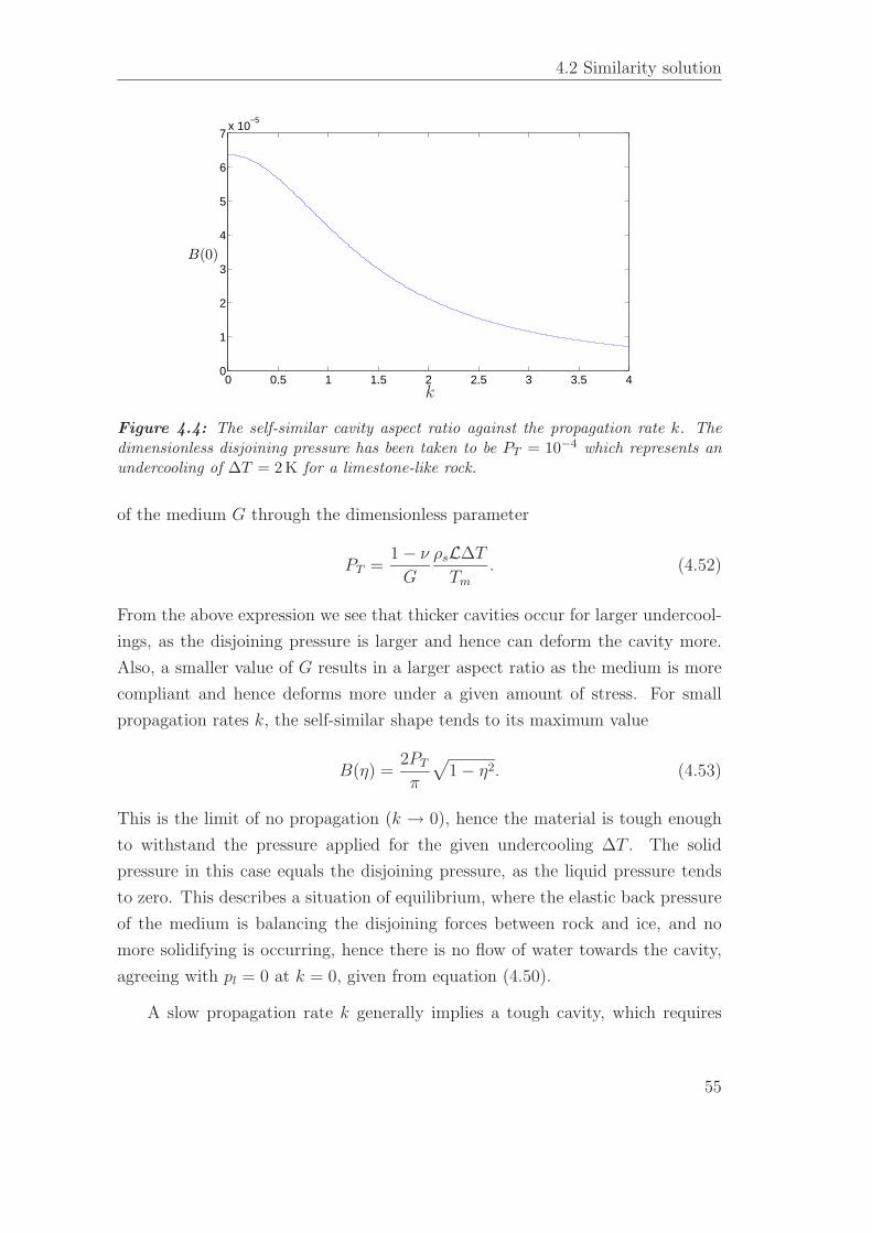
4.2 Similarity solution
0 0.5 1 1.5 2 2.5 3 3.5 40
1
2
3
4
5
6
7x 10
−5
B(0)
k
Figure 4.4: The self-similar cavity aspect ratio against the propagation rate k. Thedimensionless disjoining pressure has been taken to be PT = 10−4 which represents anundercooling of ∆T = 2 K for a limestone-like rock.
of the medium G through the dimensionless parameter
PT =1 − ν
G
ρsL∆T
Tm
. (4.52)
From the above expression we see that thicker cavities occur for larger undercool-
ings, as the disjoining pressure is larger and hence can deform the cavity more.
Also, a smaller value of G results in a larger aspect ratio as the medium is more
compliant and hence deforms more under a given amount of stress. For small
propagation rates k, the self-similar shape tends to its maximum value
B(η) =2PT
π
√
1 − η2. (4.53)
This is the limit of no propagation (k → 0), hence the material is tough enough
to withstand the pressure applied for the given undercooling ∆T . The solid
pressure in this case equals the disjoining pressure, as the liquid pressure tends
to zero. This describes a situation of equilibrium, where the elastic back pressure
of the medium is balancing the disjoining forces between rock and ice, and no
more solidifying is occurring, hence there is no flow of water towards the cavity,
agreeing with pl = 0 at k = 0, given from equation (4.50).
A slow propagation rate k generally implies a tough cavity, which requires
55
4 The penny-shaped crack
a high pressure to fracture. This implies that the deformation of the cavity,
and hence the aspect ratio, is relatively large. The liquid pressure is negative as
described by equation (4.50) but with a small absolute value. This is expected,
as the process is slow enough for the water flow through the porous medium to be
sufficiently fast so that water is able to fill the opening gap between the ice and the
rock easily. In contrast, fast propagation requires larger negative pressures, and
cavitation effects can become important. Fast fracturing occurs in weak rocks
and, since not much pressure is required to fracture them, their aspect ratios
decay like 1/k2 with the propagation rate k. Here, the controlling process is the
ability of water to flow to the freezing front at the rate required to sustain the
propagation. In general, the parameter k is related to how tough the medium
is, with large values of k corresponding to weak materials. As the radius of the
cavity is
R(t) = k
(Π
µ
G
1 − ν
)
t1/2, (4.54)
we see that the extent of the crack also depends on other material parameters,
such as the permeability Π and the shear modulus G. For example, in a very im-
permeable medium, the flow towards the solidification front is heavily constrained
and hence the growth of the cavity is slow. This results in small crack extents
for a given time t. Similarly, if a medium is very compliant (i.e. G is small),
the cavity deforms more under pressure, requiring a lot of water to freeze for the
pressure to be sustained. This results in slower propagation.
Secondly, it is interesting to note that this problem produces small aspect
ratios for the propagating cavities. Even for slow propagation, a crack of radius
1cm is only about 1µm thick, hence the aspect ratio is of the order of 10−4. We
have ignored effects of curvature-melting on the near-flat ice surface, but these
effects can become important at the highly curved ice tips. For elliptic-shaped
ice, the curvature at the tip is given by
κ =R(t)
b(0, t)2=
π2
16c1/2P 2T
(2 + k2)2
kt−1/2 ∼ 6 · 107 (2 + k2)2
k|t|−1/2cm−1, (4.55)
where |t| is the elapsed time in sec. We have used parameters appropriate for a
limestone. For an undercooling of ∆T , the Gibbs-Thompson relation given by
56
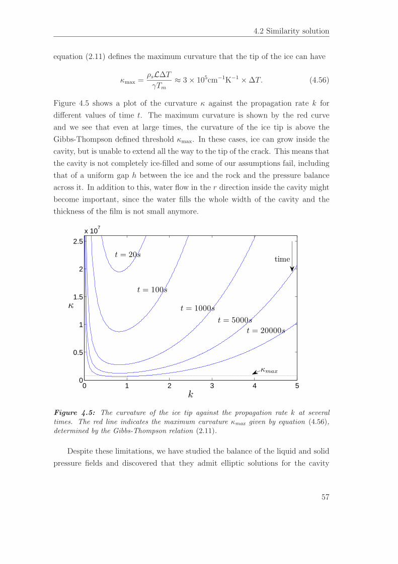
4.2 Similarity solution
equation (2.11) defines the maximum curvature that the tip of the ice can have
κmax =ρsL∆T
γTm
≈ 3 × 105cm−1K−1 × ∆T. (4.56)
Figure 4.5 shows a plot of the curvature κ against the propagation rate k for
different values of time t. The maximum curvature is shown by the red curve
and we see that even at large times, the curvature of the ice tip is above the
Gibbs-Thompson defined threshold κmax. In these cases, ice can grow inside the
cavity, but is unable to extend all the way to the tip of the crack. This means that
the cavity is not completely ice-filled and some of our assumptions fail, including
that of a uniform gap h between the ice and the rock and the pressure balance
across it. In addition to this, water flow in the r direction inside the cavity might
become important, since the water fills the whole width of the cavity and the
thickness of the film is not small anymore.
0 1 2 3 4 50
0.5
1
1.5
2
2.5
x 107
k
κ
κmax
t = 20s
t = 100s
t = 1000s
t = 5000s
t = 20000s
time
Figure 4.5: The curvature of the ice tip against the propagation rate k at severaltimes. The red line indicates the maximum curvature κmax given by equation (4.56),determined by the Gibbs-Thompson relation (2.11).
Despite these limitations, we have studied the balance of the liquid and solid
pressure fields and discovered that they admit elliptic solutions for the cavity
57
4 The penny-shaped crack
shape for uniform pressure distributions. The family of solutions has provided
information about the aspect ratio of the cavities and indicated that curvature-
melting phenomena can play an important role in determining the extent of the
ice inside the cavity. We have also derived useful results about the relation be-
tween cavity thickness and propagation rate and discussed the processes that
dominate slow and fast propagation. We now aim to improve our model to close
the problem by determining the propagation variable k and including the crite-
rion for the propagation of the cavity. Analytic solutions are unlikely to be found
for non-uniform pressure distributions. In addition to this, there will likely be
further complications when determining the propagation rate from the tip condi-
tion (4.15). We therefore aim to develop a numerical method to solve the system
of integral equations (4.11) and (4.27) together with the pressure balance (4.28).
The analytic solution obtained in this section can be used as a test for the numer-
ical results and the method can then be adjusted to solve for more complicated
situations.
4.3 Numerical approach
Concentrating on the pressure balance equation and the scales that it dictates
has given us a family of self-similar elliptic solutions. We have ignored the tip
condition which needs to be taken into account in order for the propagation rate
k to be determined. Instead of solving for the liquid pressure field directly, under
the assumption of uniform distribution, we develop a numerical method for the
integral equations, which we will first apply to the similarity solution (4.35) -
(4.37) and compare the results against the analytic solution just found. We note
that at σ = η the kernel of (4.35) has a pole singularity, while the kernel of (4.36)
has a log singularity. Any numerical schemes that we employ will have to be able
to deal with these singularities.
4.3.1 Method 1: Linear spline
The idea here is to extract the tip behaviour described by equation (4.15) and
then represent the remaining part of B(η) by using a linear spline. Even though
58
4.3 Numerical approach
the tip equation isn’t used in this test problem, we want our method to be easily
generalized to include the tip behaviour later. To do this, we divide [0, 1] into N
intervals of equal length. We take the cavity width in each interval to be of the
form
Bn(η) =(1 − η2
)1/2fn(η), (4.57)
where fn(η) is a piecewise linear function fn(η) = αnη + βn. Then,
B′
n(η) =(1 − η2
)−1/2(αn − 2αnη
2 − βnη). (4.58)
We can write expressions for the two pressures as sums of integrals that we are
able to compute numerically. For the liquid pressure we have
Pl(η) = −k2
N∑
n=1
(αnQn + βnRn) , (4.59)
where
Qn(η) =1
π
∫ ηn+1
ηn
K
(2√
ησ
η + σ
)σ4
η + σ
dσ√1 − σ2
(4.60)
and
Rn(η) =1
π
∫ ηn+1
ηn
K
(2√
ησ
η + σ
)σ
η + σ
dσ√1 − σ2
. (4.61)
Similarly,
Ps(η) =
N∑
n=1
(αnSn + βnTn) , (4.62)
with
Sn(η) = −∫ ηn+1
ηn
M(η
σ
) 2σ2 − 1√1 − σ2
dσ
σ(4.63)
and
Tn(η) = −∫ ηn+1
ηn
M(η
σ
) dσ√1 − σ2
. (4.64)
The complete elliptic integral of the first kind K(x), appearing in both inte-
grals Qn and Rn as well as the kernel M(η/σ) of the integrals Sn and Tn, has a
logarithmic singularity at x = 1. The Matlab built-in function quadgk can deal
with such integrable singularities. In addition to this, there is a pole singularity
from the kernel M(η/σ) at σ = η. We deal with this as explained in appendix C.
We need to find the coefficients of the linear spline, αn and βn, hence we have 2N
59
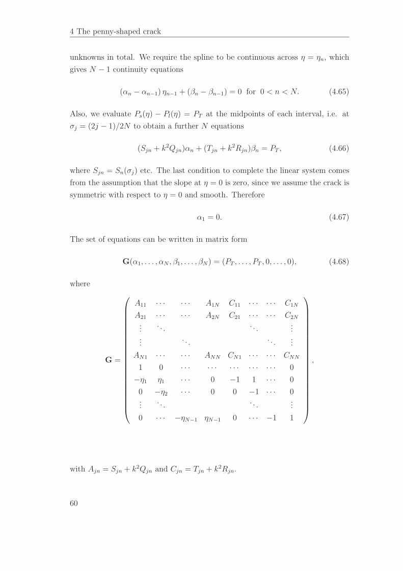
4 The penny-shaped crack
unknowns in total. We require the spline to be continuous across η = ηn, which
gives N − 1 continuity equations
(αn − αn−1) ηn−1 + (βn − βn−1) = 0 for 0 < n < N. (4.65)
Also, we evaluate Ps(η) − Pl(η) = PT at the midpoints of each interval, i.e. at
σj = (2j − 1)/2N to obtain a further N equations
(Sjn + k2Qjn)αn + (Tjn + k2Rjn)βn = PT , (4.66)
where Sjn = Sn(σj) etc. The last condition to complete the linear system comes
from the assumption that the slope at η = 0 is zero, since we assume the crack is
symmetric with respect to η = 0 and smooth. Therefore
α1 = 0. (4.67)
The set of equations can be written in matrix form
G(α1, . . . , αN , β1, . . . , βN ) = (PT , . . . , PT , 0, . . . , 0), (4.68)
where
G =
A11 · · · · · · A1N C11 · · · · · · C1N
A21 · · · · · · A2N C21 · · · · · · C2N
.... . .
. . ....
.... . . . . .
...
AN1 · · · · · · ANN CN1 · · · · · · CNN
1 0 · · · · · · · · · · · · · · · 0
−η1 η1 · · · 0 −1 1 · · · 0
0 −η2 · · · 0 0 −1 · · · 0...
. . .. . .
...
0 · · · −ηN−1 ηN−1 0 · · · −1 1
,
with Ajn = Sjn + k2Qjn and Cjn = Tjn + k2Rjn.
60
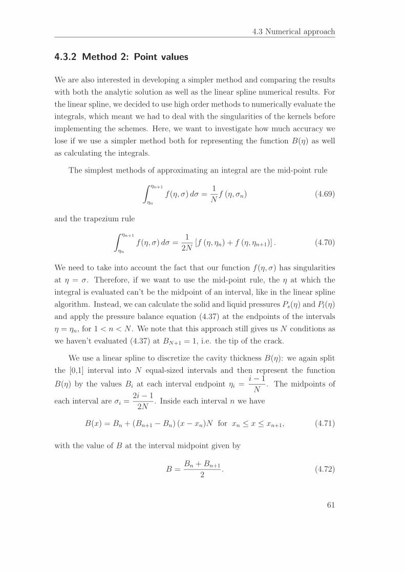
4.3 Numerical approach
4.3.2 Method 2: Point values
We are also interested in developing a simpler method and comparing the results
with both the analytic solution as well as the linear spline numerical results. For
the linear spline, we decided to use high order methods to numerically evaluate the
integrals, which meant we had to deal with the singularities of the kernels before
implementing the schemes. Here, we want to investigate how much accuracy we
lose if we use a simpler method both for representing the function B(η) as well
as calculating the integrals.
The simplest methods of approximating an integral are the mid-point rule
∫ ηn+1
ηn
f(η, σ) dσ =1
Nf (η, σn) (4.69)
and the trapezium rule
∫ ηn+1
ηn
f(η, σ) dσ =1
2N[f (η, ηn) + f (η, ηn+1)] . (4.70)
We need to take into account the fact that our function f(η, σ) has singularities
at η = σ. Therefore, if we want to use the mid-point rule, the η at which the
integral is evaluated can’t be the midpoint of an interval, like in the linear spline
algorithm. Instead, we can calculate the solid and liquid pressures Ps(η) and Pl(η)
and apply the pressure balance equation (4.37) at the endpoints of the intervals
η = ηn, for 1 < n < N . We note that this approach still gives us N conditions as
we haven’t evaluated (4.37) at BN+1 = 1, i.e. the tip of the crack.
We use a linear spline to discretize the cavity thickness B(η): we again split
the [0,1] interval into N equal-sized intervals and then represent the function
B(η) by the values Bi at each interval endpoint ηi =i − 1
N. The midpoints of
each interval are σi =2i − 1
2N. Inside each interval n we have
B(x) = Bn + (Bn+1 − Bn) (x − xn)N for xn ≤ x ≤ xn+1, (4.71)
with the value of B at the interval midpoint given by
B =Bn + Bn+1
2. (4.72)
61
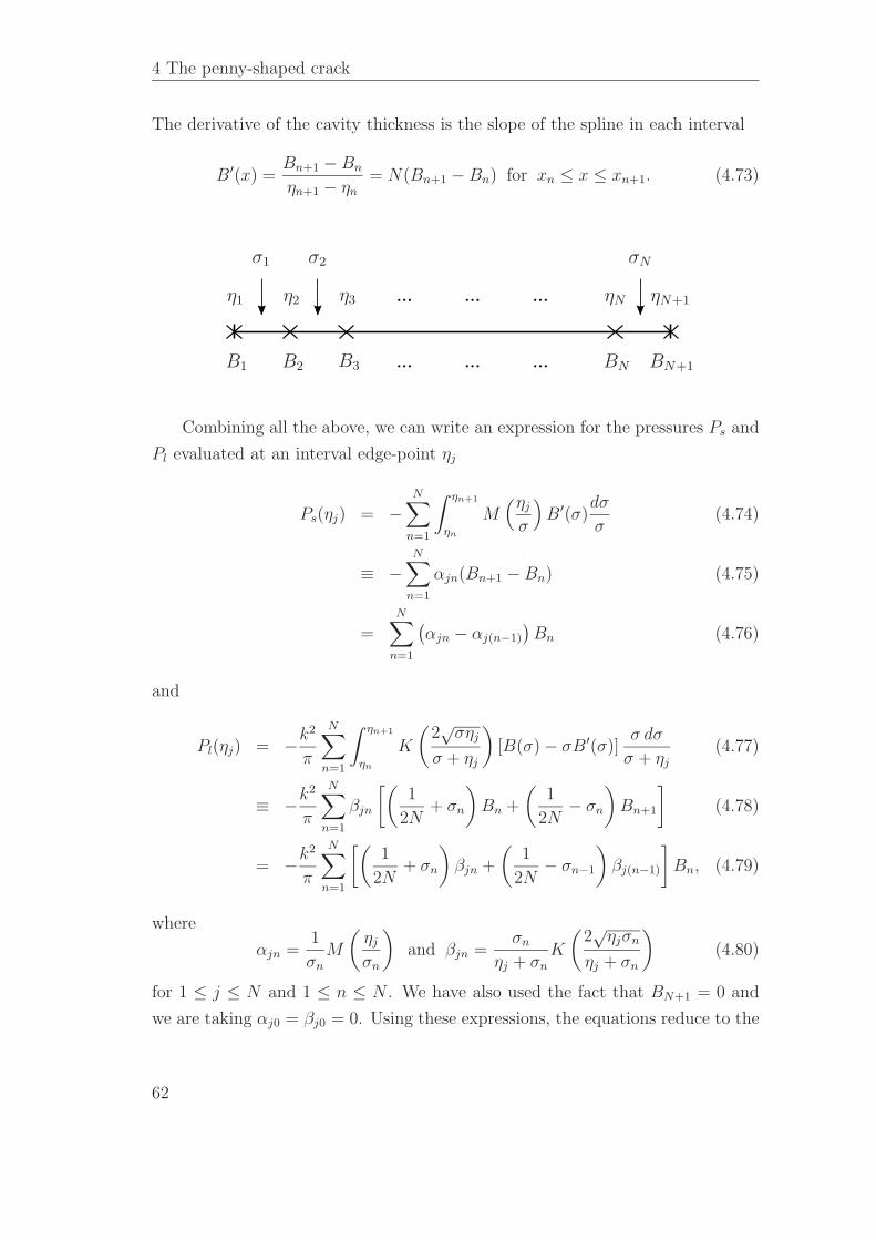
4 The penny-shaped crack
The derivative of the cavity thickness is the slope of the spline in each interval
B′(x) =Bn+1 − Bn
ηn+1 − ηn
= N(Bn+1 − Bn) for xn ≤ x ≤ xn+1. (4.73)
... ... ...
... ... ...
B1 B2 B3 BN BN+1
η1 η2 η3 ηN ηN+1
σ1 σ2 σN
Combining all the above, we can write an expression for the pressures Ps and
Pl evaluated at an interval edge-point ηj
Ps(ηj) = −N∑
n=1
∫ ηn+1
ηn
M(ηj
σ
)
B′(σ)dσ
σ(4.74)
≡ −N∑
n=1
αjn(Bn+1 − Bn) (4.75)
=
N∑
n=1
(αjn − αj(n−1)
)Bn (4.76)
and
Pl(ηj) = −k2
π
N∑
n=1
∫ ηn+1
ηn
K
(2√
σηj
σ + ηj
)
[B(σ) − σB′(σ)]σ dσ
σ + ηj
(4.77)
≡ −k2
π
N∑
n=1
βjn
[(1
2N+ σn
)
Bn +
(1
2N− σn
)
Bn+1
]
(4.78)
= −k2
π
N∑
n=1
[(1
2N+ σn
)
βjn +
(1
2N− σn−1
)
βj(n−1)
]
Bn, (4.79)
where
αjn =1
σn
M
(ηj
σn
)
and βjn =σn
ηj + σn
K
(2√
ηjσn
ηj + σn
)
(4.80)
for 1 ≤ j ≤ N and 1 ≤ n ≤ N . We have also used the fact that BN+1 = 0 and
we are taking αj0 = βj0 = 0. Using these expressions, the equations reduce to the
62
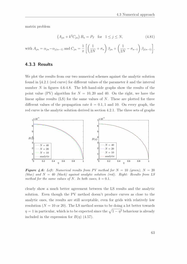
4.3 Numerical approach
matrix problem
(Ajn + k2Cjn
)Bn = PT for 1 ≤ j ≤ N, (4.81)
with Ajn = αjn−αj(n−1) and Cjn =1
π
[(1
2N+ σn
)
βjn +
(1
2N− σn−1
)
βj(n−1)
]
.
4.3.3 Results
We plot the results from our two numerical schemes against the analytic solution
found in §4.2.1 (red curve) for different values of the parameter k and the interval
number N in figures 4.6-4.8. The left-hand-side graphs show the results of the
point value (PV) algorithm for N = 10, 20 and 40. On the right, we have the
linear spline results (LS) for the same values of N . These are plotted for three
different values of the propagation rate k = 0.1, 1 and 10. On every graph, the
red curve is the analytic solution derived in section 4.2.1. The three sets of graphs
0 0.2 0.4 0.6 0.8 10
1
2
3
4
5
6
7x 10
−5
η
B(η)
N = 40
N = 20
N = 10
analytic
0 0.2 0.4 0.6 0.8 10
1
2
3
4
5
6
7x 10
−5
η
B(η)
N = 40
N = 20
N = 10
analytic
Figure 4.6: Left: Numerical results from PV method for N = 10 (green), N = 20(blue) and N = 40 (black) against analytic solution (red). Right: Results from LSmethod for the same values of N . In both cases, k = 0.1.
clearly show a much better agreement between the LS results and the analytic
solution. Even though the PV method doesn’t produce curves as close to the
analytic ones, the results are still acceptable, even for grids with relatively low
resolution (N = 10 or 20). The LS method seems to be doing a lot better towards
η = 1 in particular, which is to be expected since the√
1 − η2 behaviour is already
included in the expression for B(η) (4.57).
63
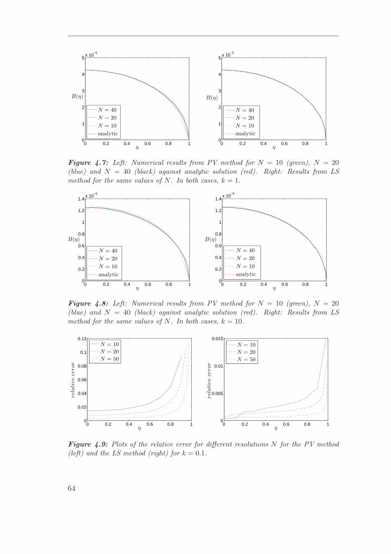
0 0.2 0.4 0.6 0.8 10
1
2
3
4
5x 10
−5
η
B(η)
N = 40
N = 20
N = 10
analytic
0 0.2 0.4 0.6 0.8 10
1
2
3
4
5x 10
−5
η
B(η)
N = 40
N = 20
N = 10
analytic
Figure 4.7: Left: Numerical results from PV method for N = 10 (green), N = 20(blue) and N = 40 (black) against analytic solution (red). Right: Results from LSmethod for the same values of N . In both cases, k = 1.
0 0.2 0.4 0.6 0.8 10
0.2
0.4
0.6
0.8
1
1.2
1.4x 10
−6
η
B(η)
N = 40
N = 20
N = 10
analytic
0 0.2 0.4 0.6 0.8 10
0.2
0.4
0.6
0.8
1
1.2
1.4x 10
−6
η
B(η)
N = 40
N = 20
N = 10
analytic
Figure 4.8: Left: Numerical results from PV method for N = 10 (green), N = 20(blue) and N = 40 (black) against analytic solution (red). Right: Results from LSmethod for the same values of N . In both cases, k = 10.
0 0.2 0.4 0.6 0.8 10
0.02
0.04
0.06
0.08
0.1
0.12
η
rela
tive
erro
r
N = 10
N = 20
N = 50
0 0.2 0.4 0.6 0.8 10
0.005
0.01
0.015
η
rela
tive
erro
r
N = 10
N = 20
N = 50
Figure 4.9: Plots of the relative error for different resolutions N for the PV method(left) and the LS method (right) for k = 0.1.
64
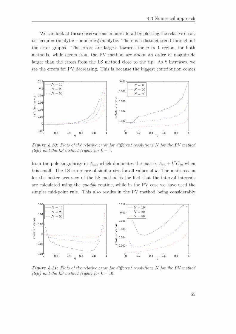
4.3 Numerical approach
We can look at these observations in more detail by plotting the relative error,
i.e. error = (analytic − numerics)/analytic. There is a distinct trend throughout
the error graphs. The errors are largest towards the η ≈ 1 region, for both
methods, while errors from the PV method are about an order of magnitude
larger than the errors from the LS method close to the tip. As k increases, we
see the errors for PV decreasing. This is because the biggest contribution comes
0 0.2 0.4 0.6 0.8 1−0.02
0
0.02
0.04
0.06
0.08
0.1
0.12
η
rela
tive
erro
r
N = 10
N = 20
N = 50
0 0.2 0.4 0.6 0.8 10
0.002
0.004
0.006
0.008
0.01
η
rela
tive
erro
r
N = 10
N = 20
N = 50
Figure 4.10: Plots of the relative error for different resolutions N for the PV method(left) and the LS method (right) for k = 1.
from the pole singularity in Ajn, which dominates the matrix Ajn + k2Cjn when
k is small. The LS errors are of similar size for all values of k. The main reason
for the better accuracy of the LS method is the fact that the interval integrals
are calculated using the quadgk routine, while in the PV case we have used the
simpler mid-point rule. This also results in the PV method being considerably
0 0.2 0.4 0.6 0.8 1−0.04
−0.02
0
0.02
0.04
0.06
η
rela
tive
erro
r
N = 10
N = 20
N = 50
0 0.2 0.4 0.6 0.8 10
0.002
0.004
0.006
0.008
0.01
0.012
η
rela
tive
erro
r
N = 10
N = 20
N = 50
Figure 4.11: Plots of the relative error for different resolutions N for the PV method(left) and the LS method (right) for k = 10.
65
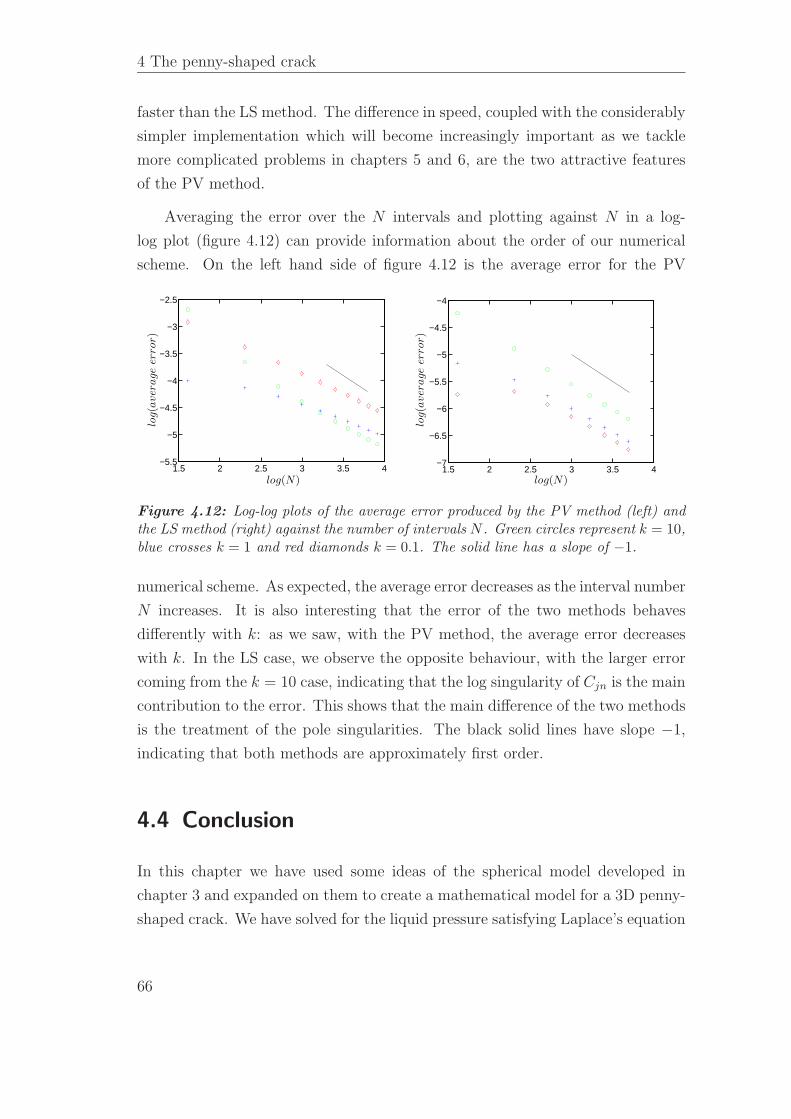
4 The penny-shaped crack
faster than the LS method. The difference in speed, coupled with the considerably
simpler implementation which will become increasingly important as we tackle
more complicated problems in chapters 5 and 6, are the two attractive features
of the PV method.
Averaging the error over the N intervals and plotting against N in a log-
log plot (figure 4.12) can provide information about the order of our numerical
scheme. On the left hand side of figure 4.12 is the average error for the PV
1.5 2 2.5 3 3.5 4−5.5
−5
−4.5
−4
−3.5
−3
−2.5
log(N)
log(a
ver
age
erro
r)
1.5 2 2.5 3 3.5 4−7
−6.5
−6
−5.5
−5
−4.5
−4
log(N)
log(a
ver
age
erro
r)
Figure 4.12: Log-log plots of the average error produced by the PV method (left) andthe LS method (right) against the number of intervals N . Green circles represent k = 10,blue crosses k = 1 and red diamonds k = 0.1. The solid line has a slope of −1.
numerical scheme. As expected, the average error decreases as the interval number
N increases. It is also interesting that the error of the two methods behaves
differently with k: as we saw, with the PV method, the average error decreases
with k. In the LS case, we observe the opposite behaviour, with the larger error
coming from the k = 10 case, indicating that the log singularity of Cjn is the main
contribution to the error. This shows that the main difference of the two methods
is the treatment of the pole singularities. The black solid lines have slope −1,
indicating that both methods are approximately first order.
4.4 Conclusion
In this chapter we have used some ideas of the spherical model developed in
chapter 3 and expanded on them to create a mathematical model for a 3D penny-
shaped crack. We have solved for the liquid pressure satisfying Laplace’s equation
66
4.4 Conclusion
in the porous medium and for the solid pressure governed by linear elasticity. The
two integral equations obtained have been combined through a pressure balance
across the premelted film. We solved the problem of uniform distribution of pres-
sures along the cavity analytically, and obtained solutions describing the propa-
gation of the cavity when the only process limiting the fracturing is the supply
of water. The propagation rate k was not determined by the pressure balance
alone, and hence a family of solutions for different values of k was found. The
theory of linear elasticity predicts the behaviour of the tip of a thin crack but we
saw that the relation cannot be incorporated in the similarity solution framework
described in this chapter.
Despite this, the study of the analytic family of solutions has provided us with
interesting conclusions about the effect that different parameters of the problem
such as the elastic modulus and the permeability of the medium, as well as the
undercooling of the system, have on the characteristics of the cavity. In particu-
lar, small aspect ratios were observed for typical parameters of rocks. In addition
to this, the analytic solution has enabled us to compare different numerical ap-
proaches for the solution of the problem, which will become useful in the next
chapters. The understanding we have obtained from this chapter will be used in
determining the important features our model should include.
67

Chapter 5
A similarity solution in a warming
environment
In chapter 4, we discussed the growth of ice in a penny-shaped cavity and looked at
the shape of those cracks and their evolution with time. We took the surrounding
environment to be undercooled to some fixed temperature T∞ < Tm, where Tm
is the melting temperature measured at some pressure pm = p∞. We found
that the propagation rate cannot be determined by the balance of the solid and
liquid pressures alone. In this chapter, we will incorporate the condition on the
tip propagation as described by equation (4.15). We also allow for temperature
variations inside the cavity and the rock, which describes the system in a more
realistic way. Irrespective of the temperature field, a constant undercooling of
the far field ∆T = Tm − T∞ implies a non-decaying temperature field, i.e. a non-
decaying disjoining pressure pT , as can be seen from equation (4.27). Through the
69
5 A similarity solution in a warming environment
pressure balance (4.28) we deduce that this implies non-decaying liquid and solid
pressure fields which, as in the previous chapter, lead to a balance between the
width and the length scales W ∼ L. This length scale balance cannot incorporate
the parabolic shape imposed by the tip condition (4.15), which is likely to make
the similarity solution break down.
The problem of a non-decaying disjoining pressure can be addressed by con-
sidering a warming environment, with the undercooling determined by a power
law of the form ∆T = Ht−α, where α > 0. This describes a supercooled system
which is warming up to Tm asymptotically. It overcomes the problem of constant
undercooling and we shall see that it provides us with the opportunity to develop
a similarity solution including the dynamics of the tip for a specific power law
α. This, used together with time-dependent results derived later, can provide an
interesting insight into the long-term behaviour of the fracture. In nature, the far-
field temperatures will vary with time, so the study here can provide interesting
insight on how this variation affects the fracturing.
5.1 The governing equations
Our extended problem is based on the model described in chapter 4, with a few
modifications to allow for temperature variations in the far field as well as the non-
uniform temperature field inside the rock and cavity. We will also consider the
Gibbs–Thompson effect of curvature-induced melting of ice, since we discovered
at the end of chapter 4 that it could potentially play an important role. Therefore,
we assume that the ice in the cavity only extends up to r = λR, where λ ∈ [0, 1],
with the rest of the cavity filled with water. A sketch of the cavity is shown in
Figure 5.1. The pressure field in the surrounding elastic medium can be expressed
in terms of the cavity shape, as in chapter 4,
ps(r, t) = − 2
πm−
∫ R(t)
0
M∗
(r
s
) ∂b
∂s
ds
s, (5.1)
where m = G/(1 − ν).
The water pressure satisfies Laplace’s equation in the porous medium. There
is a water flux q(r, t) towards the cavity and, since the crack is long and thin,
70
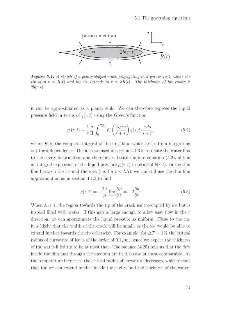
5.1 The governing equations
r
z
2b(r, t)ice
porous medium
R(t)
Figure 5.1: A sketch of a penny-shaped crack propagating in a porous rock, where thetip is at r = R(t) and the ice extends to r = λR(t). The thickness of the cavity is2b(r, t).
it can be approximated as a planar sink. We can therefore express the liquid
pressure field in terms of q(r, t) using the Green’s function
pl(r, t) =1
π
µ
Π
∫ R(t)
0
K
(2√
rs
r + s
)
q(s, t)s ds
s + r, (5.2)
where K is the complete integral of the first kind which arises from integrating
out the θ dependence. The idea we used in section 4.1.3 is to relate the water flux
to the cavity deformation and therefore, substituting into equation (5.2), obtain
an integral expression of the liquid pressure pl(r, t) in terms of b(r, t). In the thin
film between the ice and the rock (i.e. for r < λR), we can still use the thin film
approximation as in section 4.1.3 to find
q(r, t) = −2Π
µlimz→0
∂p
∂z= −2
∂b
∂t. (5.3)
When λ < 1, the region towards the tip of the crack isn’t occupied by ice but is
instead filled with water. If this gap is large enough to allow easy flow in the r
direction, we can approximate the liquid pressure as uniform. Close to the tip,
it is likely that the width of the crack will be small, as the ice would be able to
extend further towards the tip otherwise. For example, for ∆T = 1 K the critical
radius of curvature of ice is of the order of 0.1 µm, hence we expect the thickness
of the water-filled tip to be at most that. The balance (4.25) tells us that the flow
inside the film and through the medium are in this case at most comparable. As
the temperature increases, the critical radius of curvature decreases, which means
that the ice can extend further inside the cavity, and the thickness of the water-
71
5 A similarity solution in a warming environment
filled tip is even smaller. This indicates that the thin film approximation is valid
in the tip too. The alternative would be to use a uniform pressure distribution for
the water-filled tip, which would describe a situation in which the flow inside the
gap is quick enough to relax any pressure difference along the gap. Appendix D
gives the details of the uniform pressure approximation and compares results of
the two different schemes. We see that the difference in the results is minimal,
but the thin film approximation method is much easier to implement, as it only
uses the cavity width values as unknowns, and the linear matrix is of size N ×N
rather than 2N × 2N . For the remainder of the thesis we will therefore use
expression (5.3) to describe the flux of water inside the cavity. This means that
the liquid pressure can be written as
pl(r, t) = − 2
π
µ
Π
∫ R(t)
0
K
(2√
rs
r + s
)∂b
∂t
s ds
s + r. (5.4)
We assume that the temperature field is quasi-steady as in section 3.1, and
hence is described by Laplace’s equation
∇2T = 0. (5.5)
The Stefan condition expresses the release of latent heat from the solidification
front, which is necessary for the freezing process to continue
ρsL∂b
∂t= −kl lim
z→0
∂T
∂z. (5.6)
We define the undercooling θ(r, z, t) = T (r, z, t) − T∞(t) > 0 which decays as
r → ∞ and satisfies the same equations as T I , (5.5) and (5.6). By comparing
equations (5.3) and (5.6), and noting that both pl and θI satisfy Laplace’s equation
and decay as r → ∞, we see that the interface undercooling θI(r, t) ≈ θ(r, 0, t)
can be expressed in a similar way to pl as an integral of ∂b/∂t
θI(r, t) =2
π
ρsLkl
∫ λR(t)
0
K
(2√
rs
r + s
)∂b
∂t
s ds
s + r. (5.7)
In the special case λ = 1, we see that the temperature field is simply proportional
to the liquid pressure field θI = −ρsL
kl
Πµpl.
72
5.1 The governing equations
The balance of pressures across the premelted film is described by ps−pl = pT ,
where the solid pressure acting on the rock is balanced by the liquid pressure in
the thin film and the disjoining forces between the ice and the rock acting across
the film. For r > λR, where there is no ice, the solid pressure simply balances
the liquid pressure. Equation (4.30), taking into account the time-varying tem-
perature field, becomes
ps(r, t) − pl(r, t) =
ρsLHt−α
Tm
− ρsLTm
θI(r, t) if r ≤ λR.
0 if r > λR.
The extent of the ice is limited by the curvature at its tip, with its maximum
value given by the Gibbs–Thompson relation (2.11) evaluated at r = λR. The
ice tip is approximated as circular and hence the curvature at the tip is taken as
κ = 1/b(λR, t). The relation determining the ice extent λ is
κγ =2γ
b(λR(t), t)=
ρsLHt−α
Tm
− ρsLTm
θI(λR(t), t). (5.8)
Finally, as described in section 4.1.2, the tip propagation is governed by
b(r, t) ∼√
8
π
K
m
√R − r as r → R, (5.9)
where K is the critical stress-intensity factor (mode I), or fracture toughness, and
m = G/(1 − ν).
5.1.1 Non-dimensionalization
We scale pressures with P , length with L, width with W , time with t∗ and
temperature with θ∗ and we find the following balances of scales
P ∼ G
1 − ν
W
L(5.10)
P ∼ µ
Π
LW
t∗(5.11)
73
5 A similarity solution in a warming environment
θ∗ ∼ ρsLkl
LW
t∗(5.12)
P ∼ ρsLTm
θ∗ ∼ ρsLH
Tm
t∗−α (5.13)
1
W∼ ρsLH
Tm
t∗−α ∼ ρsLTm
θ∗ (5.14)
and
W ∼ K
mL1/2. (5.15)
The first four relations give us the balance of scales P ∼ θ∗ ∼ t∗−α, L ∼ t∗1/2
and W ∼ t∗−α+1/2 valid for any α. Furthermore, the ice-extent balance (5.14)
dictates that the thickness of the cavity should behave as W ∼ t∗α and the tip
condition (5.15) shows the relation between width and length W ∼ L1/2. The
last two conditions can only be included in the similarity solution for the special
case α = 1/4.
5.2 Special case: α = 14
Working with this special undercooling law of course limits the relevance of our
results to real-life scenarios, but there is a lot to be gained by this approach.
First of all, being able to include both the ice-extent condition as well as the tip
condition in our similarity solution makes for a very interesting problem worth
exploring. The results will give us an idea of the behaviour of the cavity shape
and growth rates for this specific case and, combined with the time-dependent
solution derived for more general conditions in chapter 6, we hope to be able to
derive some general conclusions.
When α = 1/4, the equations from section 5.1.1 describe a self-similar cavity.
The scales for pressure, width, length and temperature, P , W , L, θ∗ respectively,
are related to the time scale as follows
P =2
π
√
8
π
(Π
µ
)−1/4
Km−1/4t∗−1/4, (5.16)
θ∗ =2
π
√
8
π
(Π
µ
)3/4ρsLkl
Km−1/4t∗−1/4, (5.17)
74
5.2 Special case: α = 14
L =
(Π
µm
)1/2
t∗1/2, (5.18)
and
W =
√
8
π
(Π
µ
)1/4
Km3/4t∗1/4. (5.19)
According to these scalings, we take the cavity length to be R(t) = kt1/2,
for some k to be determined. Unlike chapter 4, the propagation rate k will
be determined here using the tip propagation condition (5.9). Then, we can
define a similarity variable η =r
kt1/2and introduce the cavity thickness variable
B(η) =b(r, t)
kt1/4, therefore mapping the cavity to [0, 1]. We also define the similarity
functions Ps(η) = t1/4ps(r, t), Pl(η) = t1/4pl(r, t) and ΘI(η) = t1/4θI(r, t). Then,
we have∂b
∂r= t−1/4B′(η) and
∂b
∂t=
k
t3/4
[1
4B(η) − 1
2ηB′(η)
]
. (5.20)
The set of equations in terms of the similarity variable becomes
Ps(η) = −∫ 1
0
M∗
(η
σ
)
B′(σ)dσ
σ, (5.21)
Pl(η) = −k2
∫ 1
0
K
(2√
ησ
η + σ
)[1
4B(σ) − 1
2σB′(σ)
]σdσ
η + σ(5.22)
ΘI(η) = k2
∫ λ
0
K
(2√
ησ
η + σ
) [1
4B(σ) − 1
2σB′(σ)
]σdσ
η + σ, (5.23)
Ps(η) =
{
Pl(η) − Π[ΘI(η) − C
]if η ≤ λ,
Pl(η) if η > λ,(5.24)
1
kB(λ)= KΠ
[C − ΘI(λ)
], (5.25)
B(η) ∼ k−1/2√
1 − η as η → 1, (5.26)
75
5 A similarity solution in a warming environment
where
C =H
Π3/4Kand
Π =ρ2
sL2Π
µklTm
K =4
π
K√2γm
H =
√π
2
(ρ2
sL2kl
γ2mT 3m
)1/4
H
. (5.27)
The last three parameters can be thought of as dimensionless permeability, frac-
ture toughness and undercooling respectively.
5.2.1 Numerical method
Two different numerical schemes were discussed in chapter 4 and the results were
compared in section 4.3.3. Here, we will use the PV (point values) method as it
gives reasonably accurate solutions even for a small number of intervals and is
simpler to implement and faster to run. In particular, it doesn’t require special
treatment of the pole singularities of the integrands of ps(r, t) and avoids long,
analytic calculations of integrals. As in section 4.3.2, we approximate the cavity
width B as a linear spline, such that the value of B at the nth interval midpoint
is given by
B =Bn + Bn+1
2(5.28)
and the spatial derivative is approximated by the slope of the spline in each
interval
B′ =Bn+1 − Bn
ηn+1 − ηn
= N (Bn+1 − Bn) . (5.29)
The ice extends to η = λ which is inside the Λth interval, say. This way, Λ
is defined by ηΛ+1 =Λ
N=
⌈λN⌉N
. The notation ⌈x⌉ is the ceiling function and
represents the smallest integer that isn’t smaller than x. With that definition, we
have ηΛ < λ ≤ ηΛ+1. We use the mid-point rule to calculate the integrals involved
in the expressions for the solid and liquid pressure and temperature fields. We
76
5.2 Special case: α = 14
evaluate these expressions at the interval endpoints η = ηj, 1 ≤ j ≤ N , to find
Ps(ηj) = µj1B1 +N∑
n=2
[µjn − µj(n−1)
]Bn, (5.30)
Pl(ηj) = −k2λj1B1 − k2
N∑
n=2
[λjn + νj(n−1)
]Bn (5.31)
and
ΘI(ηj) = k2λj1B1 + k2
Λ−1∑
n=2
[λjn + νj(n−1)
]Bn + k2νj(Λ−1)BΛ +
+k2Iλj BΛ + k2Jλ
j BΛ+1, (5.32)
with
µjn =1
σn
M∗
(ηj
σn
)
, (5.33)
λjn = K
(2√
ηjσn
ηj + σn
)σn
σn + ηj
(1
8N+
σn
2
)
, (5.34)
νjn = K
(2√
ηjσn
ηj + σn
)σn
σn + ηj
(1
8N− σn
2
)
. (5.35)
The last two terms from the expression for ΘI(ηj) (5.32) come from the integral
over (ηΛ, λ), which is the ice-occupied part of the Λth interval. They are given by
Iλj = K
(2√
ηjσλ
ηj + σλ
)σλ
σλ + ηj
[1
8(NηΛ+1 − Nλ + 1)(λ − ηΛ)−
− 1
4(NηΛ+1 − Nλ − 1)(λ + ηΛ)
]
(5.36)
and
Jλj = K
(2√
ηjσλ
ηj + σλ
)σλ
σλ + ηj
[1
8N(λ − ηΛ)2 − 1
4N(λ2 − η2
Λ)
]
, (5.37)
where σλ = (ηλ +λ)/2. The three expressions are related via the pressure balance
77
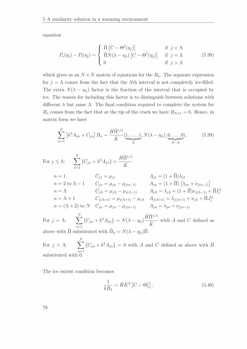
5 A similarity solution in a warming environment
equation
Ps(ηj) − Pl(ηj) =
Π[C − ΘI(ηj)
]if j < Λ
ΠN(λ − ηΛ)[C − ΘI(ηj)
]if j = Λ
0 if j > Λ
(5.38)
which gives us an N ×N matrix of equations for the Bn. The separate expression
for j = Λ comes from the fact that the Λth interval is not completely ice-filled.
The extra N(λ − ηΛ) factor is the fraction of the interval that is occupied by
ice. The reason for including this factor is to distinguish between solutions with
different λ but same Λ. The final condition required to complete the system for
Bn comes from the fact that at the tip of the crack we have BN+1 = 0. Hence, in
matrix form we have
N∑
n=1
[k2Ajn + Cjn
]Bn =
HΠ1/4
K(1, . . . , 1︸ ︷︷ ︸
Λ
, N(λ − ηΛ), 0, . . . , 0︸ ︷︷ ︸
N−Λ
). (5.39)
For j ≤ Λ:N∑
n=1
(Cjn + k2Ajn
)=
HΠ1/4
K
n = 1 Cj1 = µj1 Aj1 = (1 + Π)λj1
n = 2 to Λ − 1 Cjn = µjn − µj(n−1) Ajn = (1 + Π)[λjn + νj(n−1)
]
n = Λ CjΛ = µjΛ − µj(Λ−1) AjΛ = λjΛ + (1 + Π)νj(Λ−1) + ΠIλj
n = Λ + 1 Cj(Λ+1) = µj(Λ+1) − µjΛ Aj(Λ+1) = λj(Λ+1) + νjΛ + ΠJλj
n = (Λ + 2) to N Cjn = µjn − µj(n−1) Ajn = λjn + νj(n−1)
For j = Λ:
N∑
n=1
(Cjn + k2Ajn
)= N(λ − ηΛ)
HΠ1/4
Kwith A and C defined as
above with Π substituted with Πλ = N(λ − ηΛ)Π.
For j > Λ:N∑
n=1
(Cjn + k2Ajn
)= 0 with A and C defined as above with Π
substituted with 0.
The ice extent condition becomes
1
kBλ
= HK2[C − ΘI
λ
], (5.40)
78
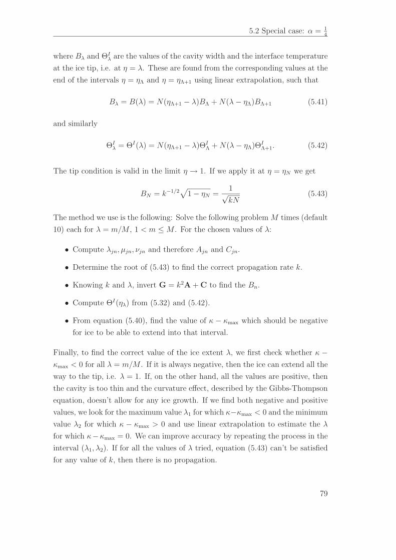
5.2 Special case: α = 14
where Bλ and ΘIλ are the values of the cavity width and the interface temperature
at the ice tip, i.e. at η = λ. These are found from the corresponding values at the
end of the intervals η = ηΛ and η = ηΛ+1 using linear extrapolation, such that
Bλ = B(λ) = N(ηΛ+1 − λ)BΛ + N(λ − ηΛ)BΛ+1 (5.41)
and similarly
ΘIλ = ΘI(λ) = N(ηΛ+1 − λ)ΘI
Λ + N(λ − ηΛ)ΘIΛ+1. (5.42)
The tip condition is valid in the limit η → 1. If we apply it at η = ηN we get
BN = k−1/2√
1 − ηN =1√kN
(5.43)
The method we use is the following: Solve the following problem M times (default
10) each for λ = m/M , 1 < m ≤ M . For the chosen values of λ:
• Compute λjn, µjn, νjn and therefore Ajn and Cjn.
• Determine the root of (5.43) to find the correct propagation rate k.
• Knowing k and λ, invert G = k2A + C to find the Bn.
• Compute ΘI(ηλ) from (5.32) and (5.42).
• From equation (5.40), find the value of κ − κmax which should be negative
for ice to be able to extend into that interval.
Finally, to find the correct value of the ice extent λ, we first check whether κ −κmax < 0 for all λ = m/M . If it is always negative, then the ice can extend all the
way to the tip, i.e. λ = 1. If, on the other hand, all the values are positive, then
the cavity is too thin and the curvature effect, described by the Gibbs-Thompson
equation, doesn’t allow for any ice growth. If we find both negative and positive
values, we look for the maximum value λ1 for which κ−κmax < 0 and the minimum
value λ2 for which κ − κmax > 0 and use linear extrapolation to estimate the λ
for which κ−κmax = 0. We can improve accuracy by repeating the process in the
interval (λ1, λ2). If for all the values of λ tried, equation (5.43) can’t be satisfied
for any value of k, then there is no propagation.
79
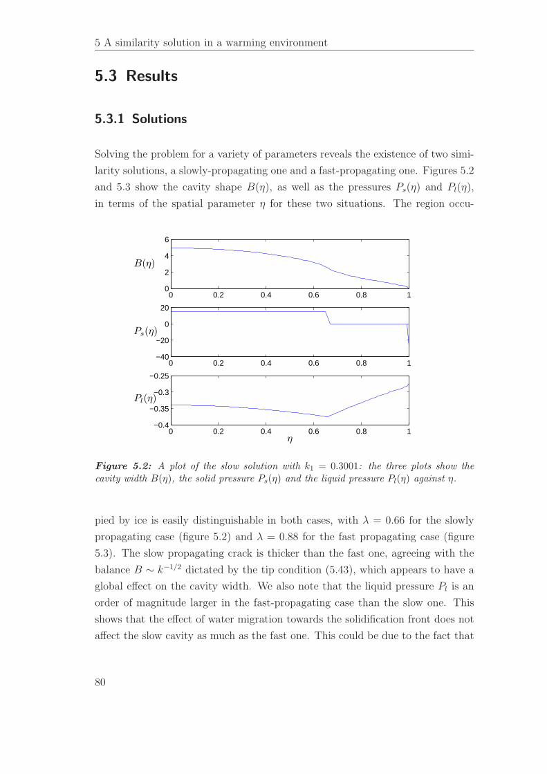
5 A similarity solution in a warming environment
5.3 Results
5.3.1 Solutions
Solving the problem for a variety of parameters reveals the existence of two simi-
larity solutions, a slowly-propagating one and a fast-propagating one. Figures 5.2
and 5.3 show the cavity shape B(η), as well as the pressures Ps(η) and Pl(η),
in terms of the spatial parameter η for these two situations. The region occu-
0 0.2 0.4 0.6 0.8 10
2
4
6
B(η)
0 0.2 0.4 0.6 0.8 1−40
−20
0
20
Ps(η)
0 0.2 0.4 0.6 0.8 1−0.4
−0.35
−0.3
−0.25
Pl(η)
η
Figure 5.2: A plot of the slow solution with k1 = 0.3001: the three plots show thecavity width B(η), the solid pressure Ps(η) and the liquid pressure Pl(η) against η.
pied by ice is easily distinguishable in both cases, with λ = 0.66 for the slowly
propagating case (figure 5.2) and λ = 0.88 for the fast propagating case (figure
5.3). The slow propagating crack is thicker than the fast one, agreeing with the
balance B ∼ k−1/2 dictated by the tip condition (5.43), which appears to have a
global effect on the cavity width. We also note that the liquid pressure Pl is an
order of magnitude larger in the fast-propagating case than the slow one. This
shows that the effect of water migration towards the solidification front does not
affect the slow cavity as much as the fast one. This could be due to the fact that
80
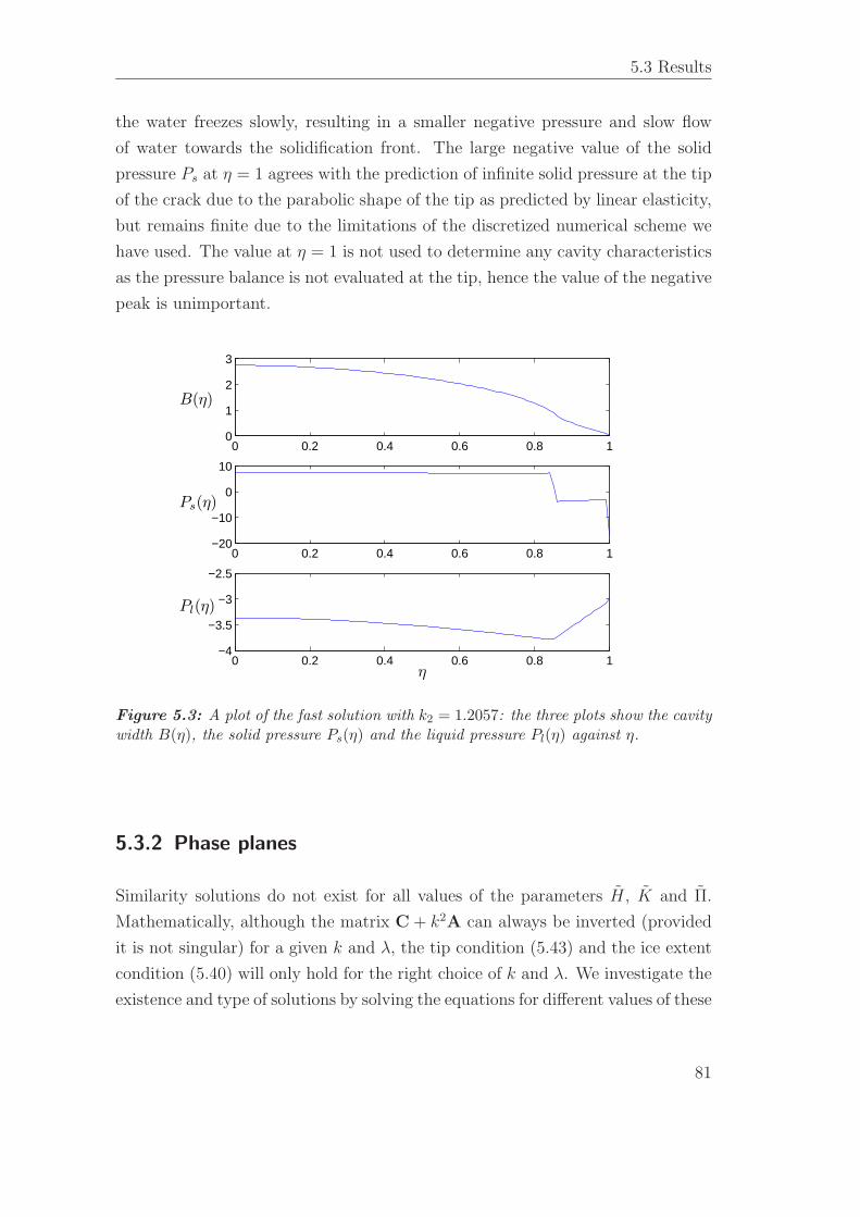
5.3 Results
the water freezes slowly, resulting in a smaller negative pressure and slow flow
of water towards the solidification front. The large negative value of the solid
pressure Ps at η = 1 agrees with the prediction of infinite solid pressure at the tip
of the crack due to the parabolic shape of the tip as predicted by linear elasticity,
but remains finite due to the limitations of the discretized numerical scheme we
have used. The value at η = 1 is not used to determine any cavity characteristics
as the pressure balance is not evaluated at the tip, hence the value of the negative
peak is unimportant.
0 0.2 0.4 0.6 0.8 10
1
2
3
B(η)
0 0.2 0.4 0.6 0.8 1−20
−10
0
10
Ps(η)
0 0.2 0.4 0.6 0.8 1−4
−3.5
−3
−2.5
Pl(η)
η
Figure 5.3: A plot of the fast solution with k2 = 1.2057: the three plots show the cavitywidth B(η), the solid pressure Ps(η) and the liquid pressure Pl(η) against η.
5.3.2 Phase planes
Similarity solutions do not exist for all values of the parameters H, K and Π.
Mathematically, although the matrix C + k2A can always be inverted (provided
it is not singular) for a given k and λ, the tip condition (5.43) and the ice extent
condition (5.40) will only hold for the right choice of k and λ. We investigate the
existence and type of solutions by solving the equations for different values of these
81
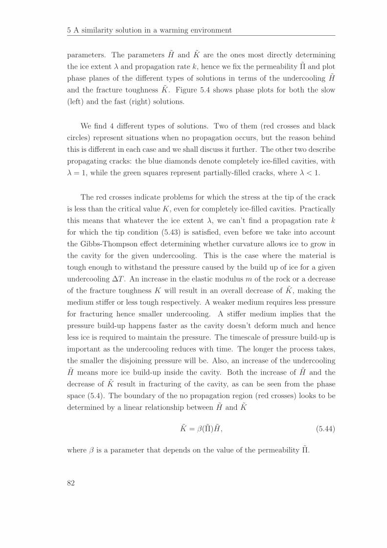
5 A similarity solution in a warming environment
parameters. The parameters H and K are the ones most directly determining
the ice extent λ and propagation rate k, hence we fix the permeability Π and plot
phase planes of the different types of solutions in terms of the undercooling H
and the fracture toughness K. Figure 5.4 shows phase plots for both the slow
(left) and the fast (right) solutions.
We find 4 different types of solutions. Two of them (red crosses and black
circles) represent situations when no propagation occurs, but the reason behind
this is different in each case and we shall discuss it further. The other two describe
propagating cracks: the blue diamonds denote completely ice-filled cavities, with
λ = 1, while the green squares represent partially-filled cracks, where λ < 1.
The red crosses indicate problems for which the stress at the tip of the crack
is less than the critical value K, even for completely ice-filled cavities. Practically
this means that whatever the ice extent λ, we can’t find a propagation rate k
for which the tip condition (5.43) is satisfied, even before we take into account
the Gibbs-Thompson effect determining whether curvature allows ice to grow in
the cavity for the given undercooling. This is the case where the material is
tough enough to withstand the pressure caused by the build up of ice for a given
undercooling ∆T . An increase in the elastic modulus m of the rock or a decrease
of the fracture toughness K will result in an overall decrease of K, making the
medium stiffer or less tough respectively. A weaker medium requires less pressure
for fracturing hence smaller undercooling. A stiffer medium implies that the
pressure build-up happens faster as the cavity doesn’t deform much and hence
less ice is required to maintain the pressure. The timescale of pressure build-up is
important as the undercooling reduces with time. The longer the process takes,
the smaller the disjoining pressure will be. Also, an increase of the undercooling
H means more ice build-up inside the cavity. Both the increase of H and the
decrease of K result in fracturing of the cavity, as can be seen from the phase
space (5.4). The boundary of the no propagation region (red crosses) looks to be
determined by a linear relationship between H and K
K = β(Π)H, (5.44)
where β is a parameter that depends on the value of the permeability Π.
82
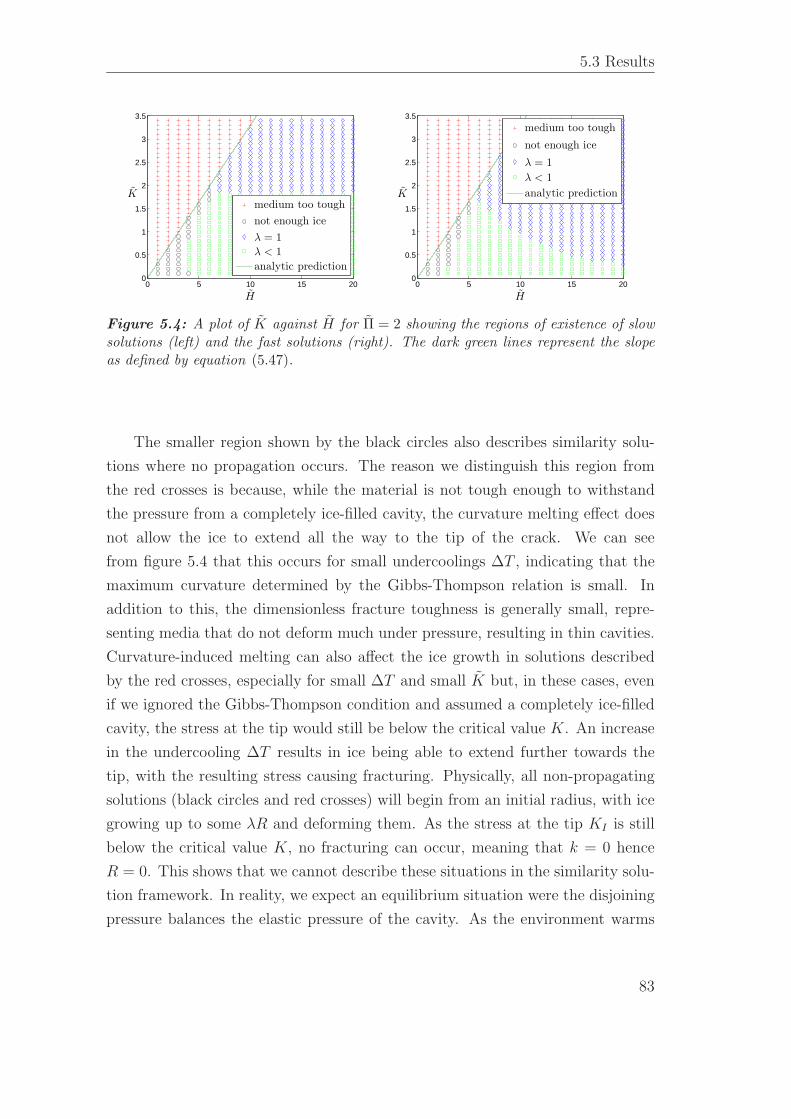
5.3 Results
0 5 10 15 200
0.5
1
1.5
2
2.5
3
3.5
H
K
medium too tough
not enough ice
λ = 1
λ < 1
analytic prediction
0 5 10 15 200
0.5
1
1.5
2
2.5
3
3.5
H
K
medium too tough
not enough ice
λ = 1
λ < 1
analytic prediction
Figure 5.4: A plot of K against H for Π = 2 showing the regions of existence of slowsolutions (left) and the fast solutions (right). The dark green lines represent the slopeas defined by equation (5.47).
The smaller region shown by the black circles also describes similarity solu-
tions where no propagation occurs. The reason we distinguish this region from
the red crosses is because, while the material is not tough enough to withstand
the pressure from a completely ice-filled cavity, the curvature melting effect does
not allow the ice to extend all the way to the tip of the crack. We can see
from figure 5.4 that this occurs for small undercoolings ∆T , indicating that the
maximum curvature determined by the Gibbs-Thompson relation is small. In
addition to this, the dimensionless fracture toughness is generally small, repre-
senting media that do not deform much under pressure, resulting in thin cavities.
Curvature-induced melting can also affect the ice growth in solutions described
by the red crosses, especially for small ∆T and small K but, in these cases, even
if we ignored the Gibbs-Thompson condition and assumed a completely ice-filled
cavity, the stress at the tip would still be below the critical value K. An increase
in the undercooling ∆T results in ice being able to extend further towards the
tip, with the resulting stress causing fracturing. Physically, all non-propagating
solutions (black circles and red crosses) will begin from an initial radius, with ice
growing up to some λR and deforming them. As the stress at the tip KI is still
below the critical value K, no fracturing can occur, meaning that k = 0 hence
R = 0. This shows that we cannot describe these situations in the similarity solu-
tion framework. In reality, we expect an equilibrium situation were the disjoining
pressure balances the elastic pressure of the cavity. As the environment warms
83
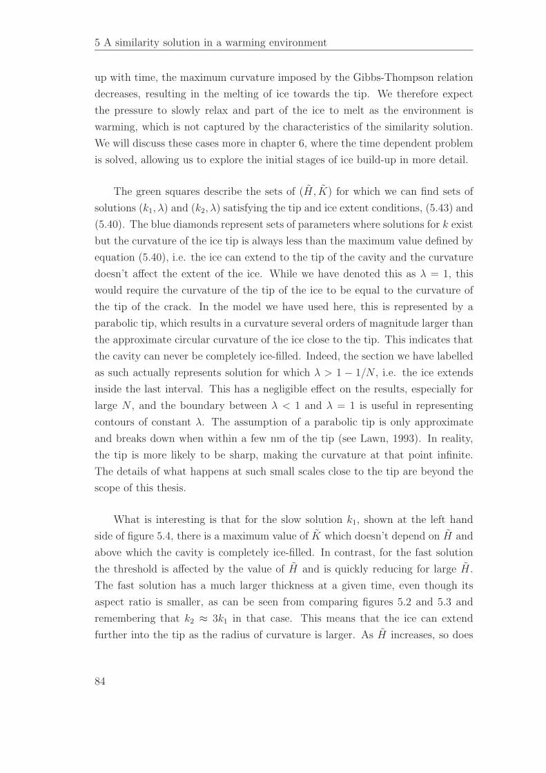
5 A similarity solution in a warming environment
up with time, the maximum curvature imposed by the Gibbs-Thompson relation
decreases, resulting in the melting of ice towards the tip. We therefore expect
the pressure to slowly relax and part of the ice to melt as the environment is
warming, which is not captured by the characteristics of the similarity solution.
We will discuss these cases more in chapter 6, where the time dependent problem
is solved, allowing us to explore the initial stages of ice build-up in more detail.
The green squares describe the sets of (H, K) for which we can find sets of
solutions (k1, λ) and (k2, λ) satisfying the tip and ice extent conditions, (5.43) and
(5.40). The blue diamonds represent sets of parameters where solutions for k exist
but the curvature of the ice tip is always less than the maximum value defined by
equation (5.40), i.e. the ice can extend to the tip of the cavity and the curvature
doesn’t affect the extent of the ice. While we have denoted this as λ = 1, this
would require the curvature of the tip of the ice to be equal to the curvature of
the tip of the crack. In the model we have used here, this is represented by a
parabolic tip, which results in a curvature several orders of magnitude larger than
the approximate circular curvature of the ice close to the tip. This indicates that
the cavity can never be completely ice-filled. Indeed, the section we have labelled
as such actually represents solution for which λ > 1 − 1/N , i.e. the ice extends
inside the last interval. This has a negligible effect on the results, especially for
large N , and the boundary between λ < 1 and λ = 1 is useful in representing
contours of constant λ. The assumption of a parabolic tip is only approximate
and breaks down when within a few nm of the tip (see Lawn, 1993). In reality,
the tip is more likely to be sharp, making the curvature at that point infinite.
The details of what happens at such small scales close to the tip are beyond the
scope of this thesis.
What is interesting is that for the slow solution k1, shown at the left hand
side of figure 5.4, there is a maximum value of K which doesn’t depend on H and
above which the cavity is completely ice-filled. In contrast, for the fast solution
the threshold is affected by the value of H and is quickly reducing for large H.
The fast solution has a much larger thickness at a given time, even though its
aspect ratio is smaller, as can be seen from comparing figures 5.2 and 5.3 and
remembering that k2 ≈ 3k1 in that case. This means that the ice can extend
further into the tip as the radius of curvature is larger. As H increases, so does
84

5.3 Results
the maximum possible curvature of the ice, hence it can grow further towards the
tip.
In general, a large fracture toughness K means more ice inside the cavity.
This can be seen from the phase plane of the fast solution, on the right hand
side of figure 5.4, where cavities are more ice-filled for a given undercooling as
K increases. A large fracture toughness indicates that more stress at the tip is
required for propagation, therefore higher pressure build-up inside the cavity is
needed. This pressure is provided by more water freezing, which creates a thicker
cavity, inside which the ice can extend closer to the tip. A large value of K can
also be caused by a small value of the elastic modulus m, which indicates an
elastic medium deforming considerably under pressure.
5.3.3 Stability of solutions
The stress intensity factor KI describes the stress at the tip of the crack and
is a result of the loading on the cavity walls. The crack starts to propagate if
KI reaches the critical value of the fracture toughness K, and we have steady
propagation for KI = K. This is expressed by equation (5.43) and provides
a means of determining the propagation rate k. We can also investigate how
different values of k correspond to different loadings at the tip. We define a
dimensionless stress-intensity factor K∗ scaled with the fracture toughness K.
The tip condition (5.43) now gives us the propagation rate k produced by some
general stress intensity K∗ at the tip
K∗ =√
kNBN . (5.45)
In this new formulation, quasi-steady propagation occurs for K∗ = 1, i.e. where
the stress-intensity factor is equal to the critical value. Figure 5.5 shows the
values of the stress intensity K∗ plotted against the corresponding propagation
rate, with the points of quasi-steady propagation denoted by the red squares.
We can now understand how the two solutions react to small perturbations in
propagation rates, therefore determining which solution is stable. We note that
for k1 < k < k2, the stress intensity factor is higher than its critical value and
85
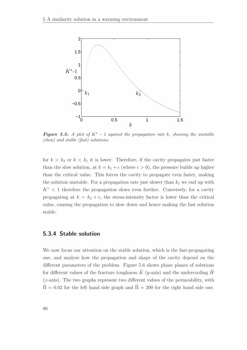
5 A similarity solution in a warming environment
0 0.5 1 1.5−1
−0.5
0
0.5
1
1.5
2
k
K∗-1
k2k1
Figure 5.5: A plot of K∗ − 1 against the propagation rate k, showing the unstable(slow) and stable (fast) solutions.
for k > k2 or k < k1 it is lower. Therefore, if the cavity propagates just faster
than the slow solution, at k = k1 + ǫ (where ǫ > 0), the pressure builds up higher
than the critical value. This forces the cavity to propagate even faster, making
the solution unstable. For a propagation rate just slower than k1 we end up with
K∗ < 1 therefore the propagation slows even further. Conversely, for a cavity
propagating at k = k2 + ǫ, the stress-intensity factor is lower than the critical
value, causing the propagation to slow down and hence making the fast solution
stable.
5.3.4 Stable solution
We now focus our attention on the stable solution, which is the fast-propagating
one, and analyse how the propagation and shape of the cavity depend on the
different parameters of the problem. Figure 5.6 shows phase planes of solutions
for different values of the fracture toughness K (y-axis) and the undercooling H
(x-axis). The two graphs represent two different values of the permeability, with
Π = 0.02 for the left hand side graph and Π = 200 for the right hand side one.
86
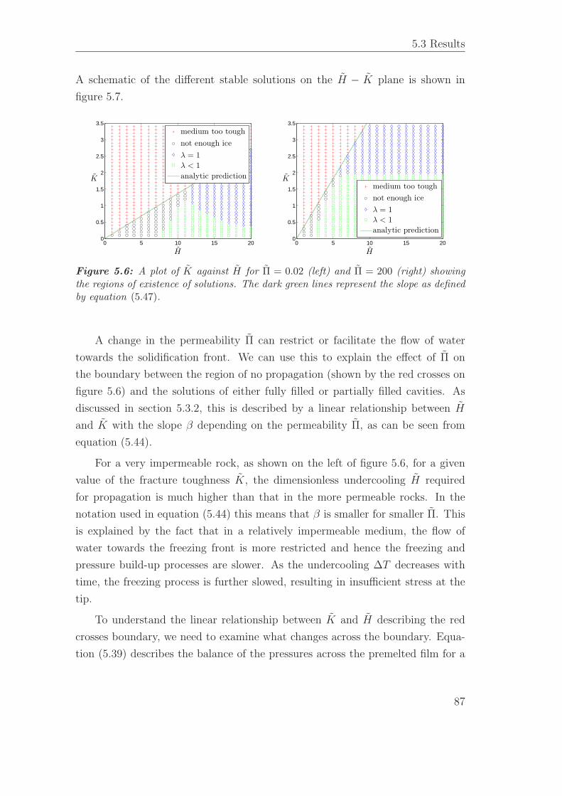
5.3 Results
A schematic of the different stable solutions on the H − K plane is shown in
figure 5.7.
0 5 10 15 200
0.5
1
1.5
2
2.5
3
3.5
H
K
medium too tough
not enough ice
λ = 1
λ < 1
analytic prediction
0 5 10 15 200
0.5
1
1.5
2
2.5
3
3.5
H
K
medium too tough
not enough ice
λ = 1
λ < 1
analytic prediction
Figure 5.6: A plot of K against H for Π = 0.02 (left) and Π = 200 (right) showingthe regions of existence of solutions. The dark green lines represent the slope as definedby equation (5.47).
A change in the permeability Π can restrict or facilitate the flow of water
towards the solidification front. We can use this to explain the effect of Π on
the boundary between the region of no propagation (shown by the red crosses on
figure 5.6) and the solutions of either fully filled or partially filled cavities. As
discussed in section 5.3.2, this is described by a linear relationship between H
and K with the slope β depending on the permeability Π, as can be seen from
equation (5.44).
For a very impermeable rock, as shown on the left of figure 5.6, for a given
value of the fracture toughness K, the dimensionless undercooling H required
for propagation is much higher than that in the more permeable rocks. In the
notation used in equation (5.44) this means that β is smaller for smaller Π. This
is explained by the fact that in a relatively impermeable medium, the flow of
water towards the freezing front is more restricted and hence the freezing and
pressure build-up processes are slower. As the undercooling ∆T decreases with
time, the freezing process is further slowed, resulting in insufficient stress at the
tip.
To understand the linear relationship between K and H describing the red
crosses boundary, we need to examine what changes across the boundary. Equa-
tion (5.39) describes the balance of the pressures across the premelted film for a
87
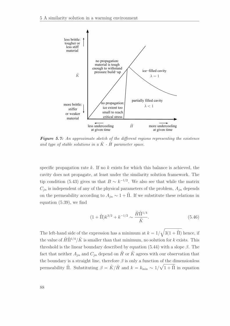
5 A similarity solution in a warming environment
less brittle:tougher orless stiffmaterial
less undercoolingat given time
more undercoolingat given time
no propagation:material is tough
enough to withstand pressure build−up
partially filled cavity
ice−filled cavity
no propagation:
ice extent too
small to reach
critical stress
more brittle:
stiffer
or weaker
material
λ < 1
λ = 1K
H
Figure 5.7: An approximate sketch of the different regions representing the existence
and type of stable solutions in a K - H parameter space.
specific propagation rate k. If no k exists for which this balance is achieved, the
cavity does not propagate, at least under the similarity solution framework. The
tip condition (5.43) gives us that B ∼ k−1/2. We also see that while the matrix
Cjn is independent of any of the physical parameters of the problem, Ajn depends
on the permeability according to Ajn ∼ 1 + Π. If we substitute these relations in
equation (5.39), we find
(1 + Π)k3/2 + k−1/2 ∼ HΠ1/4
K. (5.46)
The left-hand side of the expression has a minimum at k = 1/√
3(1 + Π) hence, if
the value of HΠ1/4/K is smaller than that minimum, no solution for k exists. This
threshold is the linear boundary described by equation (5.44) with a slope β. The
fact that neither Ajn and Cjn depend on H or K agrees with our observation that
the boundary is a straight line, therefore β is only a function of the dimensionless
permeability Π. Substituting β = K/H and k = kmin ∼ 1/√
1 + Π in equation
88
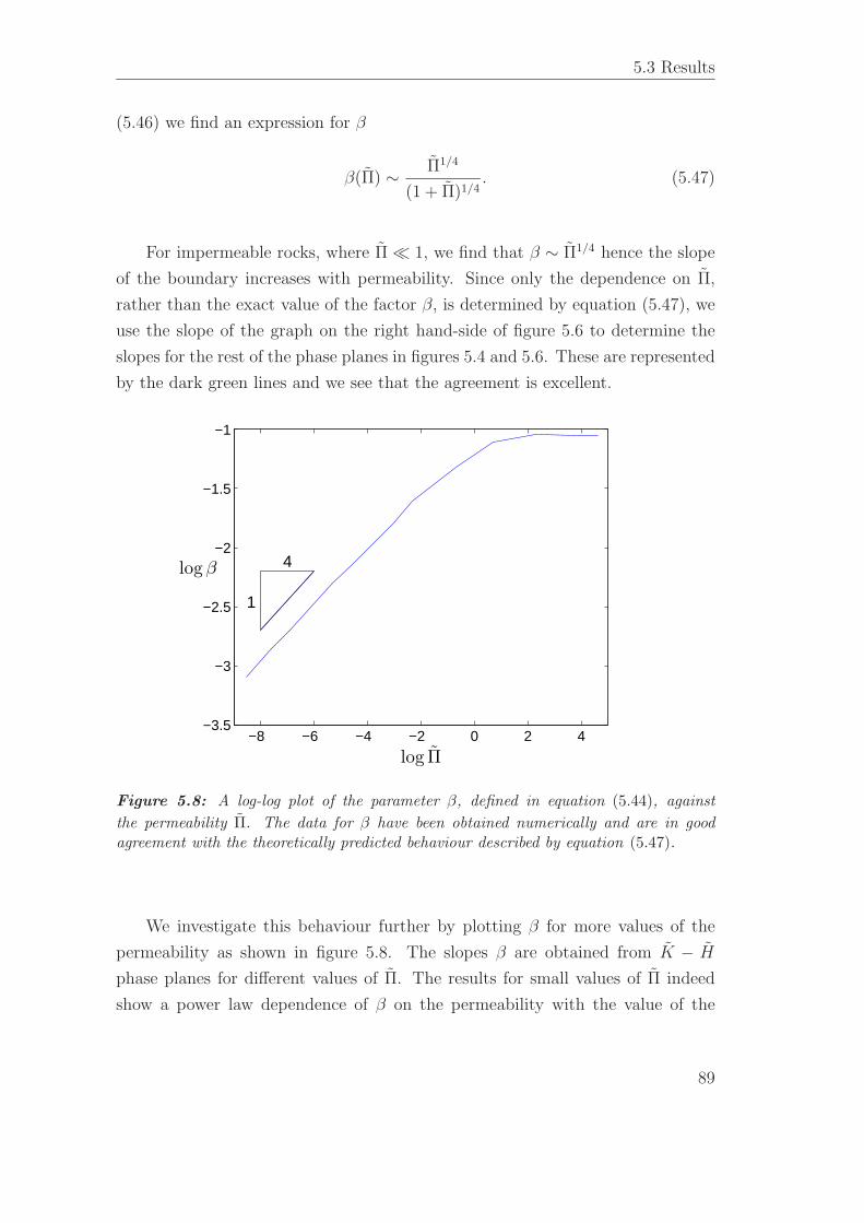
5.3 Results
(5.46) we find an expression for β
β(Π) ∼ Π1/4
(1 + Π)1/4. (5.47)
For impermeable rocks, where Π ≪ 1, we find that β ∼ Π1/4 hence the slope
of the boundary increases with permeability. Since only the dependence on Π,
rather than the exact value of the factor β, is determined by equation (5.47), we
use the slope of the graph on the right hand-side of figure 5.6 to determine the
slopes for the rest of the phase planes in figures 5.4 and 5.6. These are represented
by the dark green lines and we see that the agreement is excellent.
−8 −6 −4 −2 0 2 4−3.5
−3
−2.5
−2
−1.5
−1
log Π
logβ
1
4
Figure 5.8: A log-log plot of the parameter β, defined in equation (5.44), against
the permeability Π. The data for β have been obtained numerically and are in goodagreement with the theoretically predicted behaviour described by equation (5.47).
We investigate this behaviour further by plotting β for more values of the
permeability as shown in figure 5.8. The slopes β are obtained from K − H
phase planes for different values of Π. The results for small values of Π indeed
show a power law dependence of β on the permeability with the value of the
89
5 A similarity solution in a warming environment
power matching the theoretically predicted value of 1/4 well. As the permeability
increases, the value of the slope β tends to a constant, as is predicted by equation
(5.47) for Π ≫ 1. Physically this means that for a large enough permeability, the
availability of water supply doesn’t limit the propagation of the cavity. The region
of no propagation becomes smaller as the permeability increases but tends to a
constant for Π ≫ 1. For these permeable rocks, the propagation is only limited
by the amount of undercooling, and whether there can be enough ice growth to
cause the stress at the tip to reach the critical value K.
The effect of permeability Π
Comparing the two graphs in figure 5.6, we notice that the permeability Π strongly
affects the boundary between the λ = 1 solutions (blue diamonds) and the λ < 1
solutions (green squares). In particular, as the permeability Π decreases, solutions
with the same H and K can become ice-filled.
Figure 5.9 shows the cavity thickness Π−1/4B(η), the solid and liquid pressures
Π−1/4Ps,l(η) and the undercooling of the ice boundary Π3/4(ΘI(η) − C
), i.e. the
dimensionless T I − Tm, against the spatial variable η. These functions have been
plotted for two different values of the permeability, Π = 2 (blue solid curve) and
Π = 20 (red dashed curve). The more permeable case, described by the dashed
curve, has a smaller aspect ratio. We know from our analysis in section 5.2 that
the width of the cavity W scales with Π1/4 while the length scales with Π1/2. As
the permeability increases, both width and length increase, making the cavity
longer and thicker, but the aspect ratio decreases, meaning the cavity becomes
more slender. Despite this, the ice extent λ is smaller than in the impermeable
case, which agrees with our observations from figure 5.6. This can be explained
by considering the temperature inside the cavity in both cases: figure 5.9 shows
that for the permeable one, the cavity is much warmer, making the maximum
allowed ice curvature (dictated by the Gibbs-Thompson relation (5.40)) smaller.
Figure 5.10 shows that the propagation rate k decreases as the permeability
increases. To understand this further, we look at how the radius of the crack is
expressed in its dimensional form
R(t) =
(Π
µm
)1/2
kt1/2 (5.48)
90
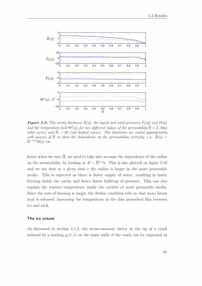
5.3 Results
0 0.1 0.2 0.3 0.4 0.5 0.6 0.7 0.8 0.9 10
1
2
B(η)
0 0.1 0.2 0.3 0.4 0.5 0.6 0.7 0.8 0.9 1−20
0
20
Ps(η)
0 0.1 0.2 0.3 0.4 0.5 0.6 0.7 0.8 0.9 1−4
−2
0
Pl(η)
0 0.1 0.2 0.3 0.4 0.5 0.6 0.7 0.8 0.9 1−10
−5
0
ΘI(η) -C
η
Figure 5.9: The cavity thickness B(η), the liquid and solid pressures Ps(η) and Pl(η)
and the temperature field ΘI(η) for two different values of the permeability Π = 2 (bluesolid curve) and Π = 20 (red dashed curve). The functions are scaled appropriatelywith powers of Π to show the dependence on the permeability correctly, e.g. B(η) =Π−1/4B(η) etc.
hence when we vary Π, we need to take into account the dependence of the radius
on the permeability by looking at R ∼ Π1/2k. This is also plotted on figure 5.10
and we see that at a given time t the radius is larger in the more permeable
media. This is expected as there is faster supply of water, resulting in faster
freezing inside the cavity and hence faster build-up of pressure. This can also
explain the warmer temperature inside the cavities of more permeable media.
Since the rate of freezing is larger, the Stefan condition tells us that more latent
heat is released, increasing the temperature in the thin premelted film between
ice and rock.
The ice extent
As discussed in section 4.1.2, the stress-intensity factor at the tip of a crack
induced by a loading ps(r, t) on the inner walls of the crack can be expressed as
91
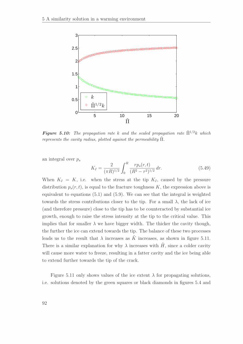
5 A similarity solution in a warming environment
5 10 15 200
0.5
1
1.5
2
2.5
3
Π
k
Π1/2k
Figure 5.10: The propagation rate k and the scaled propagation rate Π1/2k which
represents the cavity radius, plotted against the permeability Π.
an integral over ps
KI =2
(πR)1/2
∫ R
0
rps(r, t)
(R2 − r2)1/2dr. (5.49)
When KI = K, i.e. when the stress at the tip KI , caused by the pressure
distribution ps(r, t), is equal to the fracture toughness K, the expression above is
equivalent to equations (5.1) and (5.9). We can see that the integral is weighted
towards the stress contributions closer to the tip. For a small λ, the lack of ice
(and therefore pressure) close to the tip has to be counteracted by substantial ice
growth, enough to raise the stress intensity at the tip to the critical value. This
implies that for smaller λ we have bigger width. The thicker the cavity though,
the further the ice can extend towards the tip. The balance of these two processes
leads us to the result that λ increases as K increases, as shown in figure 5.11.
There is a similar explanation for why λ increases with H, since a colder cavity
will cause more water to freeze, resulting in a fatter cavity and the ice being able
to extend further towards the tip of the crack.
Figure 5.11 only shows values of the ice extent λ for propagating solutions,
i.e. solutions denoted by the green squares or black diamonds in figures 5.4 and
92
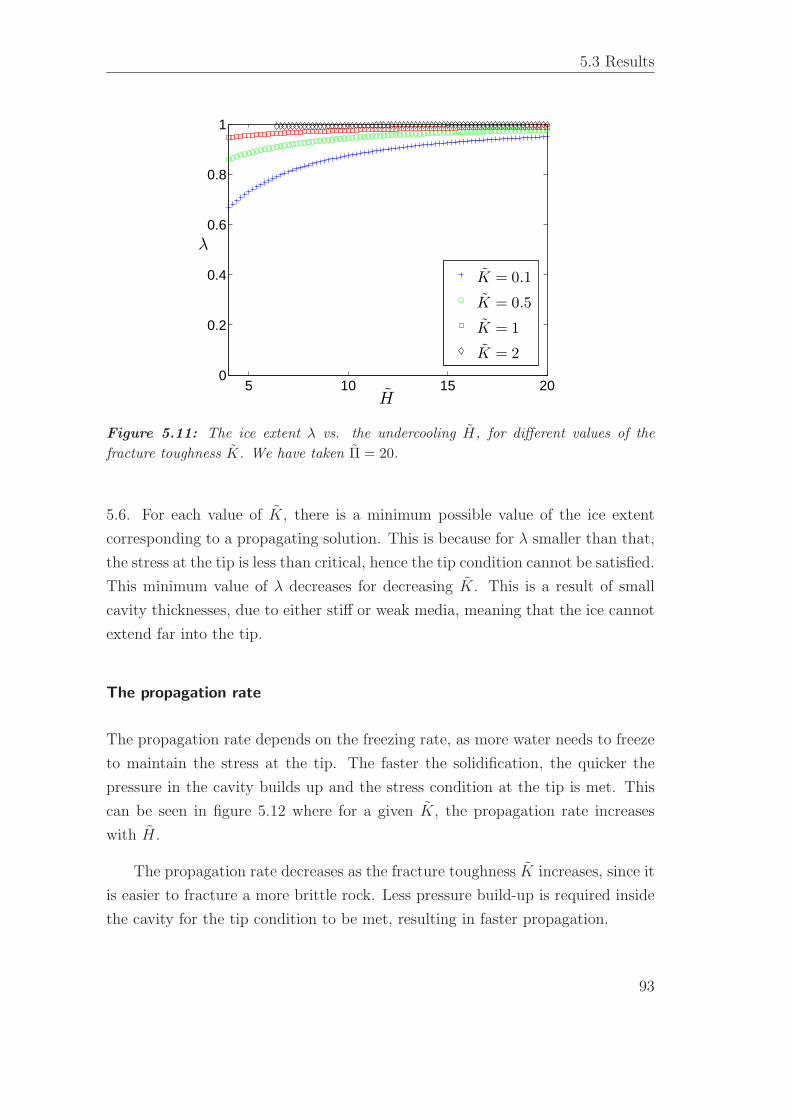
5.3 Results
5 10 15 200
0.2
0.4
0.6
0.8
1
H
λ
K = 0.1
K = 0.5
K = 1
K = 2
Figure 5.11: The ice extent λ vs. the undercooling H, for different values of the
fracture toughness K. We have taken Π = 20.
5.6. For each value of K, there is a minimum possible value of the ice extent
corresponding to a propagating solution. This is because for λ smaller than that,
the stress at the tip is less than critical, hence the tip condition cannot be satisfied.
This minimum value of λ decreases for decreasing K. This is a result of small
cavity thicknesses, due to either stiff or weak media, meaning that the ice cannot
extend far into the tip.
The propagation rate
The propagation rate depends on the freezing rate, as more water needs to freeze
to maintain the stress at the tip. The faster the solidification, the quicker the
pressure in the cavity builds up and the stress condition at the tip is met. This
can be seen in figure 5.12 where for a given K, the propagation rate increases
with H.
The propagation rate decreases as the fracture toughness K increases, since it
is easier to fracture a more brittle rock. Less pressure build-up is required inside
the cavity for the tip condition to be met, resulting in faster propagation.
93
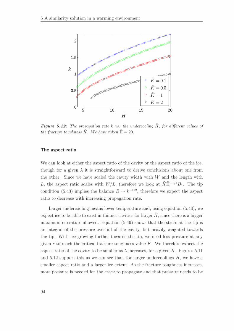
5 A similarity solution in a warming environment
5 10 15 200
0.5
1
1.5
2
H
k
K = 0.1
K = 0.5
K = 1
K = 2
Figure 5.12: The propagation rate k vs. the undercooling H, for different values of
the fracture toughness K. We have taken Π = 20.
The aspect ratio
We can look at either the aspect ratio of the cavity or the aspect ratio of the ice,
though for a given λ it is straightforward to derive conclusions about one from
the other. Since we have scaled the cavity width with W and the length with
L, the aspect ratio scales with W/L, therefore we look at KΠ−1/4B1. The tip
condition (5.43) implies the balance B ∼ k−1/2, therefore we expect the aspect
ratio to decrease with increasing propagation rate.
Larger undercooling means lower temperature and, using equation (5.40), we
expect ice to be able to exist in thinner cavities for larger H, since there is a bigger
maximum curvature allowed. Equation (5.49) shows that the stress at the tip is
an integral of the pressure over all of the cavity, but heavily weighted towards
the tip. With ice growing further towards the tip, we need less pressure at any
given r to reach the critical fracture toughness value K. We therefore expect the
aspect ratio of the cavity to be smaller as λ increases, for a given K. Figures 5.11
and 5.12 support this as we can see that, for larger undercoolings H, we have a
smaller aspect ratio and a larger ice extent. As the fracture toughness increases,
more pressure is needed for the crack to propagate and that pressure needs to be
94
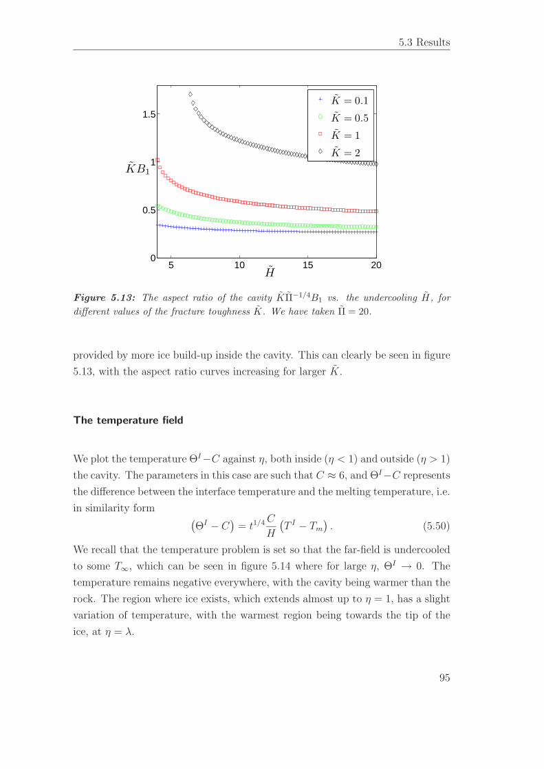
5.3 Results
5 10 15 200
0.5
1
1.5
H
KB1
K = 0.1
K = 0.5
K = 1
K = 2
Figure 5.13: The aspect ratio of the cavity KΠ−1/4B1 vs. the undercooling H, for
different values of the fracture toughness K. We have taken Π = 20.
provided by more ice build-up inside the cavity. This can clearly be seen in figure
5.13, with the aspect ratio curves increasing for larger K.
The temperature field
We plot the temperature ΘI−C against η, both inside (η < 1) and outside (η > 1)
the cavity. The parameters in this case are such that C ≈ 6, and ΘI−C represents
the difference between the interface temperature and the melting temperature, i.e.
in similarity form(ΘI − C
)= t1/4 C
H
(T I − Tm
). (5.50)
We recall that the temperature problem is set so that the far-field is undercooled
to some T∞, which can be seen in figure 5.14 where for large η, ΘI → 0. The
temperature remains negative everywhere, with the cavity being warmer than the
rock. The region where ice exists, which extends almost up to η = 1, has a slight
variation of temperature, with the warmest region being towards the tip of the
ice, at η = λ.
95
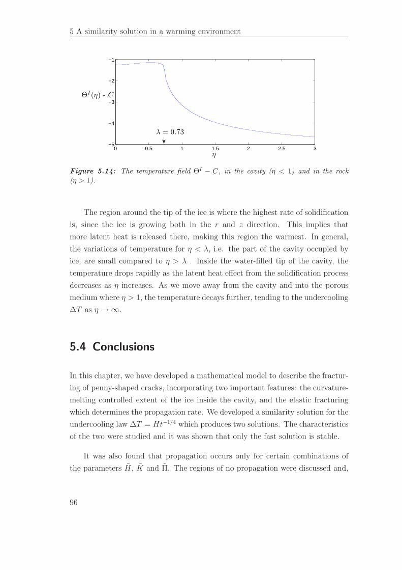
5 A similarity solution in a warming environment
0 0.5 1 1.5 2 2.5 3−5
−4
−3
−2
−1
η
ΘI(η) - C
λ = 0.73
Figure 5.14: The temperature field ΘI − C, in the cavity (η < 1) and in the rock(η > 1).
The region around the tip of the ice is where the highest rate of solidification
is, since the ice is growing both in the r and z direction. This implies that
more latent heat is released there, making this region the warmest. In general,
the variations of temperature for η < λ, i.e. the part of the cavity occupied by
ice, are small compared to η > λ . Inside the water-filled tip of the cavity, the
temperature drops rapidly as the latent heat effect from the solidification process
decreases as η increases. As we move away from the cavity and into the porous
medium where η > 1, the temperature decays further, tending to the undercooling
∆T as η → ∞.
5.4 Conclusions
In this chapter, we have developed a mathematical model to describe the fractur-
ing of penny-shaped cracks, incorporating two important features: the curvature-
melting controlled extent of the ice inside the cavity, and the elastic fracturing
which determines the propagation rate. We developed a similarity solution for the
undercooling law ∆T = Ht−1/4 which produces two solutions. The characteristics
of the two were studied and it was shown that only the fast solution is stable.
It was also found that propagation occurs only for certain combinations of
the parameters H, K and Π. The regions of no propagation were discussed and,
96
5.4 Conclusions
although their features cannot be captured by the similarity solution developed
here, an understanding of why they occur and how they behave has been es-
tablished. These will be studied further in the next chapter, where the time
dependent problem allows us to look at the initial stages of pressure build-up.
Characteristics of the stable fracturing such as the ice extent, the propagation
rate and the aspect ratio of the cavities were studied and their dependence on the
dimensionless parameters H, K and Π was discussed. This allowed us to develop
an understanding of the relative importance of the different parameters which will
help us in our studies of the time dependent model.
An interesting feature which arises from the assumption of a warming envi-
ronment is the importance of the permeability Π, which controls the time scale of
flow and water supply. Since the undercooling decreases with time, media with
low permeabilities can experience no fracturing, even for parameters for which
more permeable media would fracture. This is due to the time-dependence of the
undercooling and, since the next chapter is predominantly involved with constant
undercoolings, it is an important point to take away from this study.
97

Chapter 6
Time-dependent problem
In chapter 5 we developed a model predicting the fracturing of a crack caused
by the freezing of water in a saturated porous medium. Linear elasticity, which
predicts propagation when the stress at the tip of the cavity reaches a critical
value, is coupled with the Darcy flow and temperature field equations to produce
a system of coupled integral relations that can be solved for the shape and radius
of the cavity. A similarity solution was found for the special case of background
undercooling ∆T ∼ t−1/4. For thin cavities, the curvature at the tip of the ice can
become large. The Gibbs-Thompson relation (2.11) is taken into account when
determining the extent of the ice inside the cavity, as it defines the maximum ice
curvature for a given undercooling. We found a parameter regime for which the
ice cannot extend all the way to the tip of the crack, because of the phenomenon
of curvature-induced melting.
99
6 Time-dependent problem
Having a similarity solution that incorporates all the important features of
the problem is extremely useful and has allowed us to derive many interesting con-
clusions about how the different parameters of the problem affect the crack prop-
agation. Using the understanding we have gained, we are now better equipped
to solve the full time-dependent problem. This is important for several reasons,
not least because it allows us to consider a general undercooling law and easily
change from a uniform undercooling to a power law like the one used in chapter
5.
Furthermore, we can study not only the long-time behaviour of the crack,
where the process has developed and the pressure build-up is causing the cavity
to propagate, but also the initial stage of ice growth. This is characterized by
the stress at the tip KI being below the critical value K and therefore the crack
does not propagate. During this stage, the cavity thickness increases as a result
of the ice formation and subsequent pressure build-up, while the stress at the tip
KI approaches the critical value K. The ice extent λ is a complicated function
of the undercooling of the surrounding and the thickness of the cavity, and this
framework allows for it to vary with time. We will, in general, keep the analysis in
this chapter dimensionless, as we are mainly interested in exploring the qualitative
dependence of fracturing on the different parameters of the problem. Applications
of the theory to different rocks and soils are presented in chapter 7.
6.1 Dimensional time-dependent problem
The set-up of the problem is more or less identical to the one presented in section
5.1. We consider the surrounding environment to be undercooled to the constant
value ∆T = Tm − T∞ > 0, but note that it is straightforward to modify this to a
power law and incorporate it into our algorithm if we want to draw comparisons
with the similarity solution. As before, the solid and liquid pressure integrals are
given by
ps(r, t) = − 2
πm−
∫ R(t)
0
M∗
(r
s
) ∂b
∂s
ds
s, (6.1)
pl(r, t) = − 2
π
µ
Π
∫ R(t)
0
K
(2√
rs
r + s
)∂b
∂t
s ds
s + r, (6.2)
100
6.2 Scalings
while the temperature is
θI(r, t) = T I(r, t) − T∞ =2
π
ρsLkl
∫ λR(t)
0
K
(2√
rs
r + s
)∂b
∂t
s ds
s + r. (6.3)
These are connected via the pressure balance:
ps(r, t) − pl(r, t) =
ρsL∆T
Tm
− ρsLTm
θI(r, t) if r ≤ λR.
0 if r > λR.
(6.4)
The ice extends to r = λ(t)R(t), where the parameter λ is determined by the
Gibbs-Thompson relation
2γ
b(λR, t)=
ρsL∆T
Tm
− ρsLTm
θI(λR(t), t). (6.5)
It is important to remember that λ can vary with time, unlike in the similarity
solution frame, and hence will have to be computed at every time step. When
the stress at the tip reaches the critical value, the cavity propagates according to
b(r, t) ∼ K
m
[8(R − r)
π
]1/2
as r → R. (6.6)
6.2 Scalings
We scale the equations for pressure, length, width, temperature and time with
p∗, R0 = R(t0), W , θ∗ and t∗. The following scalings arise
W =
√
8
π
K
mR
1/20 , (6.7)
p∗ =2
π
√
8
πR
−1/20 K, (6.8)
θ∗ =2
π
√
8
πR
−1/20
ρsLΠ
µkl
K, (6.9)
t∗ =µ
ΠmR2
0. (6.10)
101
6 Time-dependent problem
The pressure balance and ice extent conditions now become
ps(r, t) − pl(r, t) =
H
K− ΠθI(r, t) if r ≤ λR
0 if r > λR
and1
b(λR, t)= K2
(
H
K− ΠθI(λR(t), t)
)
, (6.11)
where the pressures ps and pl, the temperature θI and the width b(r, t) are now
dimensionless. The new constants that we introduced Π, K and H represent the
dimensionless permeability, fracture toughness and undercooling respectively, as
in chapter 5, although their definitions are slightly different:
Π =ρ2
sL2Π
µklTm
, (6.12)
H =
√
πR0
4γm
ρsL∆T
Tm
, (6.13)
K =4
π
K√2γm
. (6.14)
We map the [0, R] interval to [0, 1] by setting η = r/R(t). Then
∂η
∂r=
1
R(t)and
∂η
∂t= −rR′(t)
R2(t). (6.15)
We also let B(η, t) = b(r, t)/R(t) in order to preserve the aspect ratio. Then
∂b(r, t)
∂r=
∂B(η, t)
∂η(6.16)
and∂b(r, t)
∂t= R(t)
∂B(η, t)
∂t+ R′(t)
(
B(η, t) − η∂B(η, t)
∂η
)
. (6.17)
Then, the equations describing the system become
Ps(η, t) = −−∫ 1
0
M(η
σ
) ∂B(σ, t)
∂σ
dσ
σ, (6.18)
102
6.3 Numerical scheme
Pl(η, t) = −∫ 1
0
K
(2√
ησ
η + σ
)
Q(σ, t)σ dσ
σ + η(6.19)
and
ΘI(η, t) =
∫ λ
0
K
(2√
ησ
η + σ
)
Q(σ, t)σ dσ
σ + η, (6.20)
where
Q(σ, t) =
{
R(t)∂B(σ, t)
∂t+ R′(t)
[
B(σ, t) − σ∂B(σ, t)
∂σ
]}
R(t). (6.21)
The pressure balance simply becomes
Ps(η, t) − Pl(η, t) =
H
K− ΠΘI(η, t) if η ≤ λ.
0 if η > λ.
The ice extent is determined by
1
R(t)B(λ, t)= K2
(
H
K− ΠΘI(λ, t)
)
(6.22)
and the condition on the crack propagation comes from
B(η, t) ∼ R(t)−1/2√
1 − η, as η → 1. (6.23)
6.3 Numerical scheme
We again split [0, 1] in N intervals. The edges of the intervals are ηn = (n− 1)/N
and the values of the cavity width there are Bn(t) = B(ηn, t). We denote the
values at the ith iteration with the superscript i so that Bin = Bn(ti). We denote
the time step by ∆t such that ti = t0 + i∆t. As the method used here is almost
identical to that in section 5.2.1, we skip the details, which can be found in
Appendix B. For a given λi and Ri, we have the following linear problem to
solve.
103
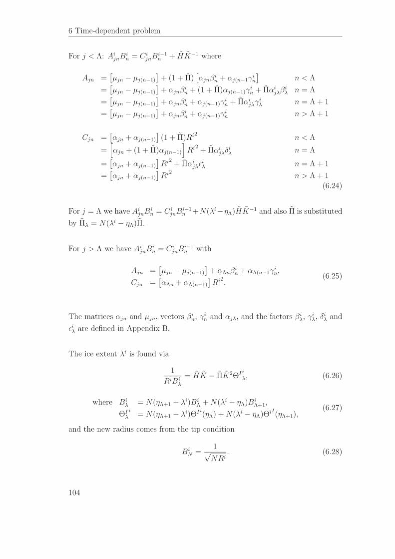
6 Time-dependent problem
For j < Λ: AijnB
in = Ci
jnBi−1n + HK−1 where
Ajn =[µjn − µj(n−1)
]+ (1 + Π)
[αjnβi
n + αj(n−1γin
]n < Λ
=[µjn − µj(n−1)
]+ αjnβ
in + (1 + Π)αj(n−1)γ
in + Παi
jλβiλ n = Λ
=[µjn − µj(n−1)
]+ αjnβ
in + αj(n−1)γ
in + Παi
jλγiλ n = Λ + 1
=[µjn − µj(n−1)
]+ αjnβ
in + αj(n−1)γ
in n > Λ + 1
Cjn =[αjn + αj(n−1)
](1 + Π)Ri2 n < Λ
=[
αjn + (1 + Π)αj(n−1)
]
Ri2 + Παijλδ
iλ n = Λ
=[αjn + αj(n−1)
]Ri2 + Παi
jλǫiλ n = Λ + 1
=[αjn + αj(n−1)
]Ri2 n > Λ + 1
(6.24)
For j = Λ we have AijnB
in = Ci
jnBi−1n +N(λi−ηΛ)HK−1 and also Π is substituted
by Πλ = N(λi − ηΛ)Π.
For j > Λ we have AijnB
in = Ci
jnBi−1n with
Ajn =[µjn − µj(n−1)
]+ αΛnβ
in + αΛ(n−1γ
in,
Cjn =[αΛn + αΛ(n−1)
]Ri2.
(6.25)
The matrices αjn and µjn, vectors βin, γi
n and αjλ, and the factors βiλ, γi
λ, δiλ and
ǫiλ are defined in Appendix B.
The ice extent λi is found via
1
RiBiλ
= HK − ΠK2ΘI i
λ, (6.26)
where Biλ = N(ηΛ+1 − λi)Bi
Λ + N(λi − ηΛ)BiΛ+1,
ΘIλ
i= N(ηΛ+1 − λi)ΘI i
(ηΛ) + N(λi − ηΛ)ΘiI(ηΛ+1),(6.27)
and the new radius comes from the tip condition
BiN =
1√NRi
. (6.28)
104
6.4 Initial condition
Technical details
We give a brief outline of the algorithm used to solve the problem described above.
• Choose initial condition
• Compute time-independent matrices µjn and αjn.
• For the ith iteration, for a number of values of λi equally spaced around
λi−1, do the following:
– Use a least squares routine to find the value of Ri that satisfies the tip
condition;
– Now that we know Ri for each of the values of λi, we can find Bin by
computing Ajn and Cjn and inverting the matrix;
– Compute the curvature at the tip of the ice using equation (6.28) for
every λi.
• We pick the largest λi for which κ − κmax < 0 (or use linear interpolation
between this and the next (positive) value to find a more accurate solution).
Figure 6.1 shows that κ − κmax is an increasing function of λi.
• We now have found the correct ice extent λi that satisfies Gibbs-Thompson.
We can now find the radius Ri that satisfies the tip condition and then solve
for the thickness Bin.
6.4 Initial condition
An advantage of solving the time-dependent problem is that we can investigate
the initial stages of ice formation and pressure build-up, rather than just looking
at the propagation at the critical state KI = K. A simple way of thinking about
how a situation like this can develop in nature is to imagine a pre-existing fault,
with some ice growing inside it. Initially, the stress at the tip is sub-critical
and hence no fracturing occurs. Instead, water keeps freezing inside the non-
propagating cavity, causing it to increase in thickness. This in turn increases the
pressure applied on the rock, and subsequently the stress at the tip. When the
critical value is reached, the propagation begins.
105
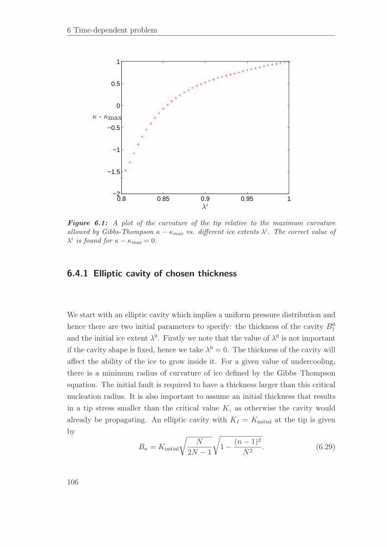
6 Time-dependent problem
0.8 0.85 0.9 0.95 1−2
−1.5
−1
−0.5
0
0.5
1
λi
κ - κmax
Figure 6.1: A plot of the curvature of the tip relative to the maximum curvatureallowed by Gibbs-Thompson κ − κmax vs. different ice extents λi. The correct value ofλi is found for κ − κmax = 0.
6.4.1 Elliptic cavity of chosen thickness
We start with an elliptic cavity which implies a uniform pressure distribution and
hence there are two initial parameters to specify: the thickness of the cavity B01
and the initial ice extent λ0. Firstly we note that the value of λ0 is not important
if the cavity shape is fixed, hence we take λ0 = 0. The thickness of the cavity will
affect the ability of the ice to grow inside it. For a given value of undercooling,
there is a minimum radius of curvature of ice defined by the Gibbs–Thompson
equation. The initial fault is required to have a thickness larger than this critical
nucleation radius. It is also important to assume an initial thickness that results
in a tip stress smaller than the critical value K, as otherwise the cavity would
already be propagating. An elliptic cavity with KI = Kinitial at the tip is given
by
Bn = Kinitial
√
N
2N − 1
√
1 − (n − 1)2
N2. (6.29)
106
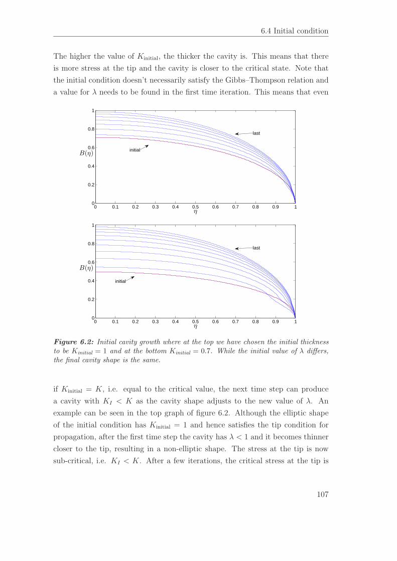
6.4 Initial condition
The higher the value of Kinitial, the thicker the cavity is. This means that there
is more stress at the tip and the cavity is closer to the critical state. Note that
the initial condition doesn’t necessarily satisfy the Gibbs–Thompson relation and
a value for λ needs to be found in the first time iteration. This means that even
0 0.1 0.2 0.3 0.4 0.5 0.6 0.7 0.8 0.9 10
0.2
0.4
0.6
0.8
1
η
B(η)initial
last
0 0.1 0.2 0.3 0.4 0.5 0.6 0.7 0.8 0.9 10
0.2
0.4
0.6
0.8
1
η
B(η)
last
initial
Figure 6.2: Initial cavity growth where at the top we have chosen the initial thicknessto be Kinitial = 1 and at the bottom Kinitial = 0.7. While the initial value of λ differs,the final cavity shape is the same.
if Kinitial = K, i.e. equal to the critical value, the next time step can produce
a cavity with KI < K as the cavity shape adjusts to the new value of λ. An
example can be seen in the top graph of figure 6.2. Although the elliptic shape
of the initial condition has Kinitial = 1 and hence satisfies the tip condition for
propagation, after the first time step the cavity has λ < 1 and it becomes thinner
closer to the tip, resulting in a non-elliptic shape. The stress at the tip is now
sub-critical, i.e. KI < K. After a few iterations, the critical stress at the tip is
107
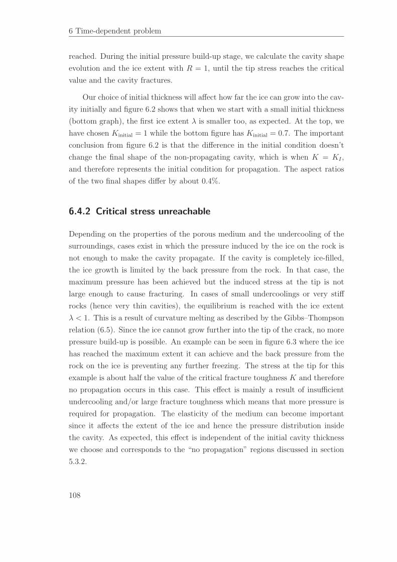
6 Time-dependent problem
reached. During the initial pressure build-up stage, we calculate the cavity shape
evolution and the ice extent with R = 1, until the tip stress reaches the critical
value and the cavity fractures.
Our choice of initial thickness will affect how far the ice can grow into the cav-
ity initially and figure 6.2 shows that when we start with a small initial thickness
(bottom graph), the first ice extent λ is smaller too, as expected. At the top, we
have chosen Kinitial = 1 while the bottom figure has Kinitial = 0.7. The important
conclusion from figure 6.2 is that the difference in the initial condition doesn’t
change the final shape of the non-propagating cavity, which is when K = KI ,
and therefore represents the initial condition for propagation. The aspect ratios
of the two final shapes differ by about 0.4%.
6.4.2 Critical stress unreachable
Depending on the properties of the porous medium and the undercooling of the
surroundings, cases exist in which the pressure induced by the ice on the rock is
not enough to make the cavity propagate. If the cavity is completely ice-filled,
the ice growth is limited by the back pressure from the rock. In that case, the
maximum pressure has been achieved but the induced stress at the tip is not
large enough to cause fracturing. In cases of small undercoolings or very stiff
rocks (hence very thin cavities), the equilibrium is reached with the ice extent
λ < 1. This is a result of curvature melting as described by the Gibbs–Thompson
relation (6.5). Since the ice cannot grow further into the tip of the crack, no more
pressure build-up is possible. An example can be seen in figure 6.3 where the ice
has reached the maximum extent it can achieve and the back pressure from the
rock on the ice is preventing any further freezing. The stress at the tip for this
example is about half the value of the critical fracture toughness K and therefore
no propagation occurs in this case. This effect is mainly a result of insufficient
undercooling and/or large fracture toughness which means that more pressure is
required for propagation. The elasticity of the medium can become important
since it affects the extent of the ice and hence the pressure distribution inside
the cavity. As expected, this effect is independent of the initial cavity thickness
we choose and corresponds to the “no propagation” regions discussed in section
5.3.2.
108
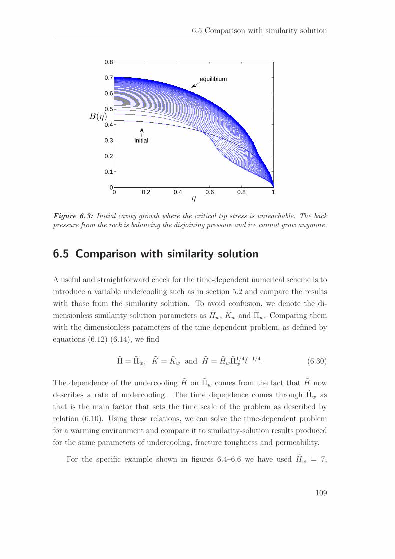
6.5 Comparison with similarity solution
0 0.2 0.4 0.6 0.8 10
0.1
0.2
0.3
0.4
0.5
0.6
0.7
0.8
η
B(η)
initial
equilibium
Figure 6.3: Initial cavity growth where the critical tip stress is unreachable. The backpressure from the rock is balancing the disjoining pressure and ice cannot grow anymore.
6.5 Comparison with similarity solution
A useful and straightforward check for the time-dependent numerical scheme is to
introduce a variable undercooling such as in section 5.2 and compare the results
with those from the similarity solution. To avoid confusion, we denote the di-
mensionless similarity solution parameters as Hw, Kw and Πw. Comparing them
with the dimensionless parameters of the time-dependent problem, as defined by
equations (6.12)-(6.14), we find
Π = Πw, K = Kw and H = HwΠ1/4w t−1/4. (6.30)
The dependence of the undercooling H on Πw comes from the fact that H now
describes a rate of undercooling. The time dependence comes through Πw as
that is the main factor that sets the time scale of the problem as described by
relation (6.10). Using these relations, we can solve the time-dependent problem
for a warming environment and compare it to similarity-solution results produced
for the same parameters of undercooling, fracture toughness and permeability.
For the specific example shown in figures 6.4–6.6 we have used Hw = 7,
109
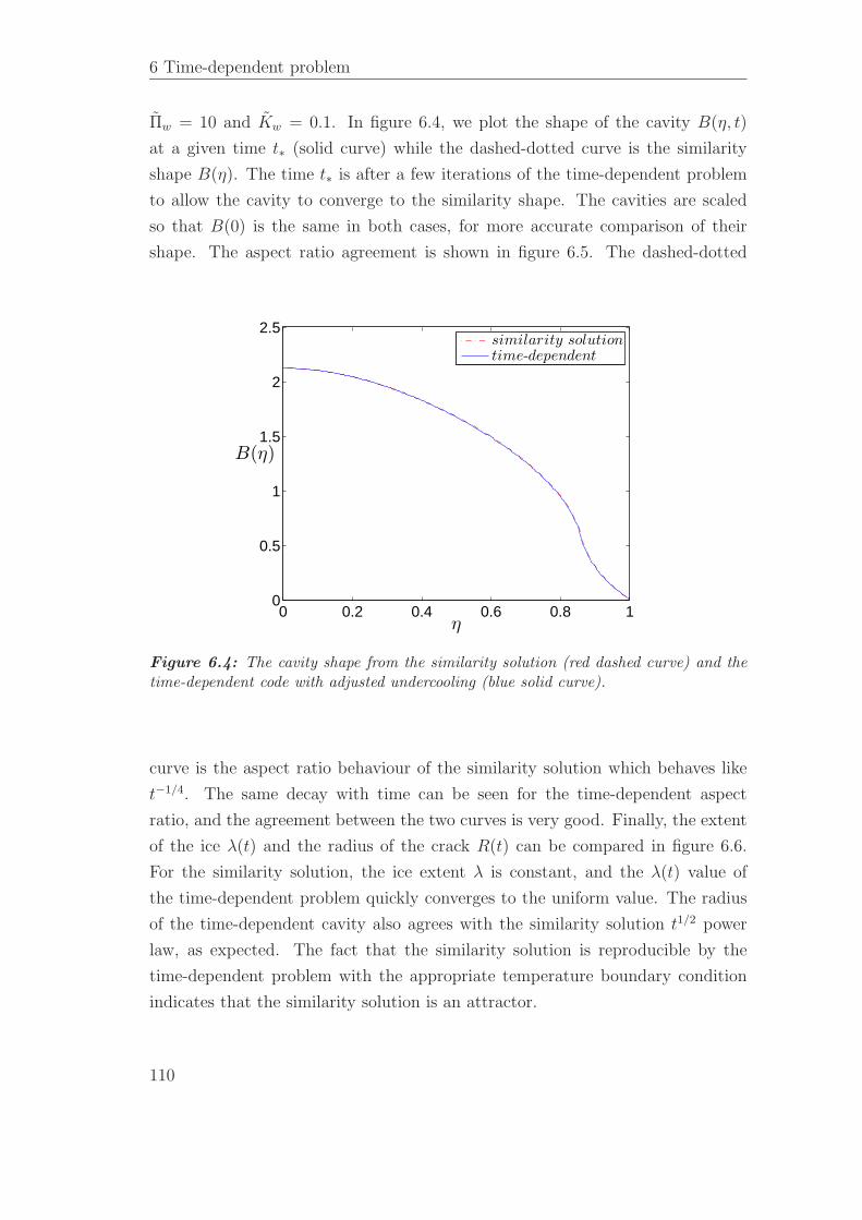
6 Time-dependent problem
Πw = 10 and Kw = 0.1. In figure 6.4, we plot the shape of the cavity B(η, t)
at a given time t∗ (solid curve) while the dashed-dotted curve is the similarity
shape B(η). The time t∗ is after a few iterations of the time-dependent problem
to allow the cavity to converge to the similarity shape. The cavities are scaled
so that B(0) is the same in both cases, for more accurate comparison of their
shape. The aspect ratio agreement is shown in figure 6.5. The dashed-dotted
0 0.2 0.4 0.6 0.8 10
0.5
1
1.5
2
2.5
B(η)
η
similarity solutiontime-dependent
Figure 6.4: The cavity shape from the similarity solution (red dashed curve) and thetime-dependent code with adjusted undercooling (blue solid curve).
curve is the aspect ratio behaviour of the similarity solution which behaves like
t−1/4. The same decay with time can be seen for the time-dependent aspect
ratio, and the agreement between the two curves is very good. Finally, the extent
of the ice λ(t) and the radius of the crack R(t) can be compared in figure 6.6.
For the similarity solution, the ice extent λ is constant, and the λ(t) value of
the time-dependent problem quickly converges to the uniform value. The radius
of the time-dependent cavity also agrees with the similarity solution t1/2 power
law, as expected. The fact that the similarity solution is reproducible by the
time-dependent problem with the appropriate temperature boundary condition
indicates that the similarity solution is an attractor.
110
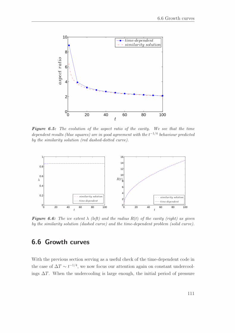
6.6 Growth curves
0 20 40 60 80 1000
2
4
6
8
10
t
asp
ect
rati
o
time-dependentsimilarity solution
Figure 6.5: The evolution of the aspect ratio of the cavity. We see that the time
dependent results (blue squares) are in good agreement with the t−1/4 behaviour predictedby the similarity solution (red dashed-dotted curve).
0 20 40 60 80 1000
0.2
0.4
0.6
0.8
1
t
λ
similarity solution
time-dependent
0 20 40 60 80 1000
2
4
6
8
10
12
14
16
t
R(t)
similarity solution
time-dependent
Figure 6.6: The ice extent λ (left) and the radius R(t) of the cavity (right) as givenby the similarity solution (dashed curve) and the time-dependent problem (solid curve).
6.6 Growth curves
With the previous section serving as a useful check of the time-dependent code in
the case of ∆T ∼ t−1/4, we now focus our attention again on constant undercool-
ings ∆T . When the undercooling is large enough, the initial period of pressure
111
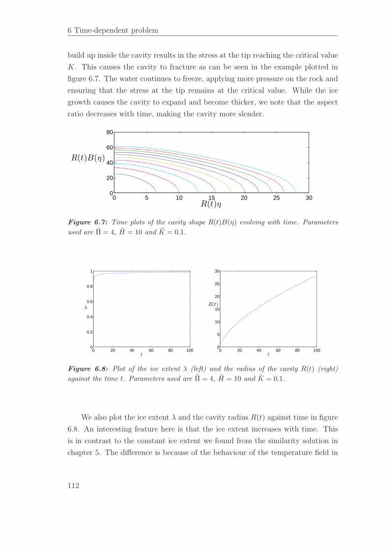
6 Time-dependent problem
build up inside the cavity results in the stress at the tip reaching the critical value
K. This causes the cavity to fracture as can be seen in the example plotted in
figure 6.7. The water continues to freeze, applying more pressure on the rock and
ensuring that the stress at the tip remains at the critical value. While the ice
growth causes the cavity to expand and become thicker, we note that the aspect
ratio decreases with time, making the cavity more slender.
0 5 10 15 20 25 300
20
40
60
80
R(t)η
R(t)B(η)
Figure 6.7: Time plots of the cavity shape R(t)B(η) evolving with time. Parameters
used are Π = 4, H = 10 and K = 0.1.
0 20 40 60 80 1000
0.2
0.4
0.6
0.8
1
t
λ
0 20 40 60 80 1000
5
10
15
20
25
30
t
R(t)
Figure 6.8: Plot of the ice extent λ (left) and the radius of the cavity R(t) (right)
against the time t. Parameters used are Π = 4, H = 10 and K = 0.1.
We also plot the ice extent λ and the cavity radius R(t) against time in figure
6.8. An interesting feature here is that the ice extent increases with time. This
is in contrast to the constant ice extent we found from the similarity solution in
chapter 5. The difference is because of the behaviour of the temperature field in
112
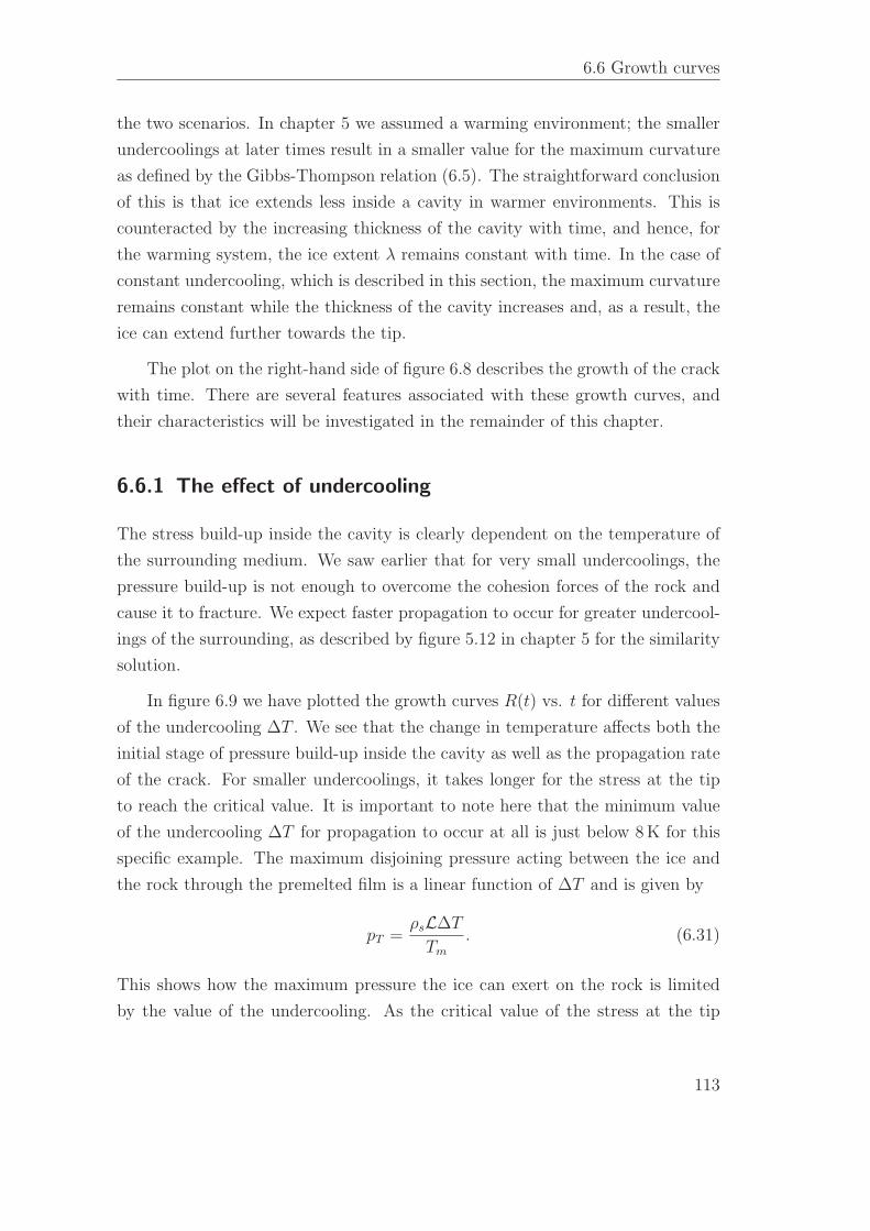
6.6 Growth curves
the two scenarios. In chapter 5 we assumed a warming environment; the smaller
undercoolings at later times result in a smaller value for the maximum curvature
as defined by the Gibbs-Thompson relation (6.5). The straightforward conclusion
of this is that ice extends less inside a cavity in warmer environments. This is
counteracted by the increasing thickness of the cavity with time, and hence, for
the warming system, the ice extent λ remains constant with time. In the case of
constant undercooling, which is described in this section, the maximum curvature
remains constant while the thickness of the cavity increases and, as a result, the
ice can extend further towards the tip.
The plot on the right-hand side of figure 6.8 describes the growth of the crack
with time. There are several features associated with these growth curves, and
their characteristics will be investigated in the remainder of this chapter.
6.6.1 The effect of undercooling
The stress build-up inside the cavity is clearly dependent on the temperature of
the surrounding medium. We saw earlier that for very small undercoolings, the
pressure build-up is not enough to overcome the cohesion forces of the rock and
cause it to fracture. We expect faster propagation to occur for greater undercool-
ings of the surrounding, as described by figure 5.12 in chapter 5 for the similarity
solution.
In figure 6.9 we have plotted the growth curves R(t) vs. t for different values
of the undercooling ∆T . We see that the change in temperature affects both the
initial stage of pressure build-up inside the cavity as well as the propagation rate
of the crack. For smaller undercoolings, it takes longer for the stress at the tip
to reach the critical value. It is important to note here that the minimum value
of the undercooling ∆T for propagation to occur at all is just below 8 K for this
specific example. The maximum disjoining pressure acting between the ice and
the rock through the premelted film is a linear function of ∆T and is given by
pT =ρsL∆T
Tm
. (6.31)
This shows how the maximum pressure the ice can exert on the rock is limited
by the value of the undercooling. As the critical value of the stress at the tip
113
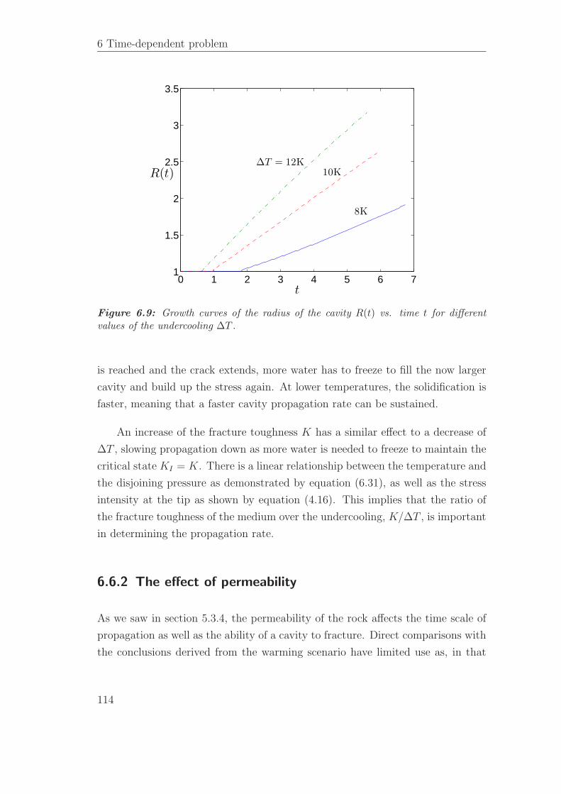
6 Time-dependent problem
0 1 2 3 4 5 6 71
1.5
2
2.5
3
3.5
t
R(t)
∆T = 12K
8K
10K
Figure 6.9: Growth curves of the radius of the cavity R(t) vs. time t for differentvalues of the undercooling ∆T .
is reached and the crack extends, more water has to freeze to fill the now larger
cavity and build up the stress again. At lower temperatures, the solidification is
faster, meaning that a faster cavity propagation rate can be sustained.
An increase of the fracture toughness K has a similar effect to a decrease of
∆T , slowing propagation down as more water is needed to freeze to maintain the
critical state KI = K. There is a linear relationship between the temperature and
the disjoining pressure as demonstrated by equation (6.31), as well as the stress
intensity at the tip as shown by equation (4.16). This implies that the ratio of
the fracture toughness of the medium over the undercooling, K/∆T , is important
in determining the propagation rate.
6.6.2 The effect of permeability
As we saw in section 5.3.4, the permeability of the rock affects the time scale of
propagation as well as the ability of a cavity to fracture. Direct comparisons with
the conclusions derived from the warming scenario have limited use as, in that
114
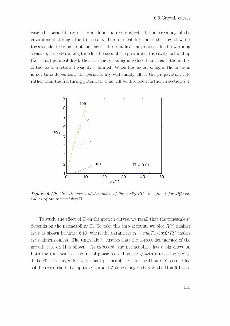
6.6 Growth curves
case, the permeability of the medium indirectly affects the undercooling of the
environment through the time scale. The permeability limits the flow of water
towards the freezing front and hence the solidification process. In the warming
scenario, if it takes a long time for the ice and the pressure in the cavity to build up
(i.e. small permeability), then the undercooling is reduced and hence the ability
of the ice to fracture the cavity is limited. When the undercooling of the medium
is not time dependent, the permeability will simply affect the propagation rate
rather than the fracturing potential. This will be discussed further in section 7.4.
0 10 20 30 40 501
2
3
4
5
6
7
8
9
c1t∗t
R(t)
Π = 0.010.1
1
100
10
Figure 6.10: Growth curves of the radius of the cavity R(t) vs. time t for differentvalues of the permeability Π.
To study the effect of Π on the growth curves, we recall that the timescale t∗
depends on the permeability Π. To take this into account, we plot R(t) against
c1t∗t as shown in figure 6.10, where the parameter c1 = mklTm/(ρ2
sL2R20) makes
c1t∗t dimensionless. The timescale t∗ ensures that the correct dependence of the
growth rate on Π is shown. As expected, the permeability has a big effect on
both the time scale of the initial phase as well as the growth rate of the cavity.
This effect is larger for very small permeabilities: in the Π = 0.01 case (blue
solid curve), the build-up time is about 5 times longer than in the Π = 0.1 case
115
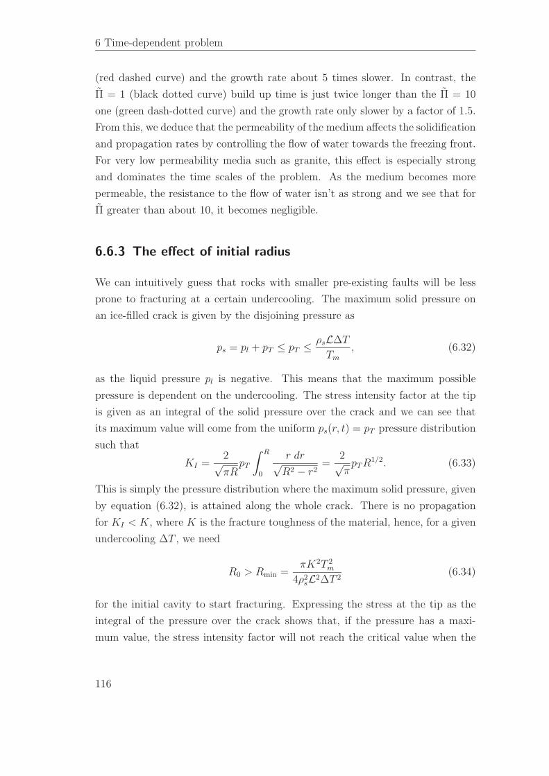
6 Time-dependent problem
(red dashed curve) and the growth rate about 5 times slower. In contrast, the
Π = 1 (black dotted curve) build up time is just twice longer than the Π = 10
one (green dash-dotted curve) and the growth rate only slower by a factor of 1.5.
From this, we deduce that the permeability of the medium affects the solidification
and propagation rates by controlling the flow of water towards the freezing front.
For very low permeability media such as granite, this effect is especially strong
and dominates the time scales of the problem. As the medium becomes more
permeable, the resistance to the flow of water isn’t as strong and we see that for
Π greater than about 10, it becomes negligible.
6.6.3 The effect of initial radius
We can intuitively guess that rocks with smaller pre-existing faults will be less
prone to fracturing at a certain undercooling. The maximum solid pressure on
an ice-filled crack is given by the disjoining pressure as
ps = pl + pT ≤ pT ≤ ρsL∆T
Tm
, (6.32)
as the liquid pressure pl is negative. This means that the maximum possible
pressure is dependent on the undercooling. The stress intensity factor at the tip
is given as an integral of the solid pressure over the crack and we can see that
its maximum value will come from the uniform ps(r, t) = pT pressure distribution
such that
KI =2√πR
pT
∫ R
0
r dr√R2 − r2
=2√π
pTR1/2. (6.33)
This is simply the pressure distribution where the maximum solid pressure, given
by equation (6.32), is attained along the whole crack. There is no propagation
for KI < K, where K is the fracture toughness of the material, hence, for a given
undercooling ∆T , we need
R0 > Rmin =πK2T 2
m
4ρ2sL2∆T 2
(6.34)
for the initial cavity to start fracturing. Expressing the stress at the tip as the
integral of the pressure over the crack shows that, if the pressure has a maxi-
mum value, the stress intensity factor will not reach the critical value when the
116
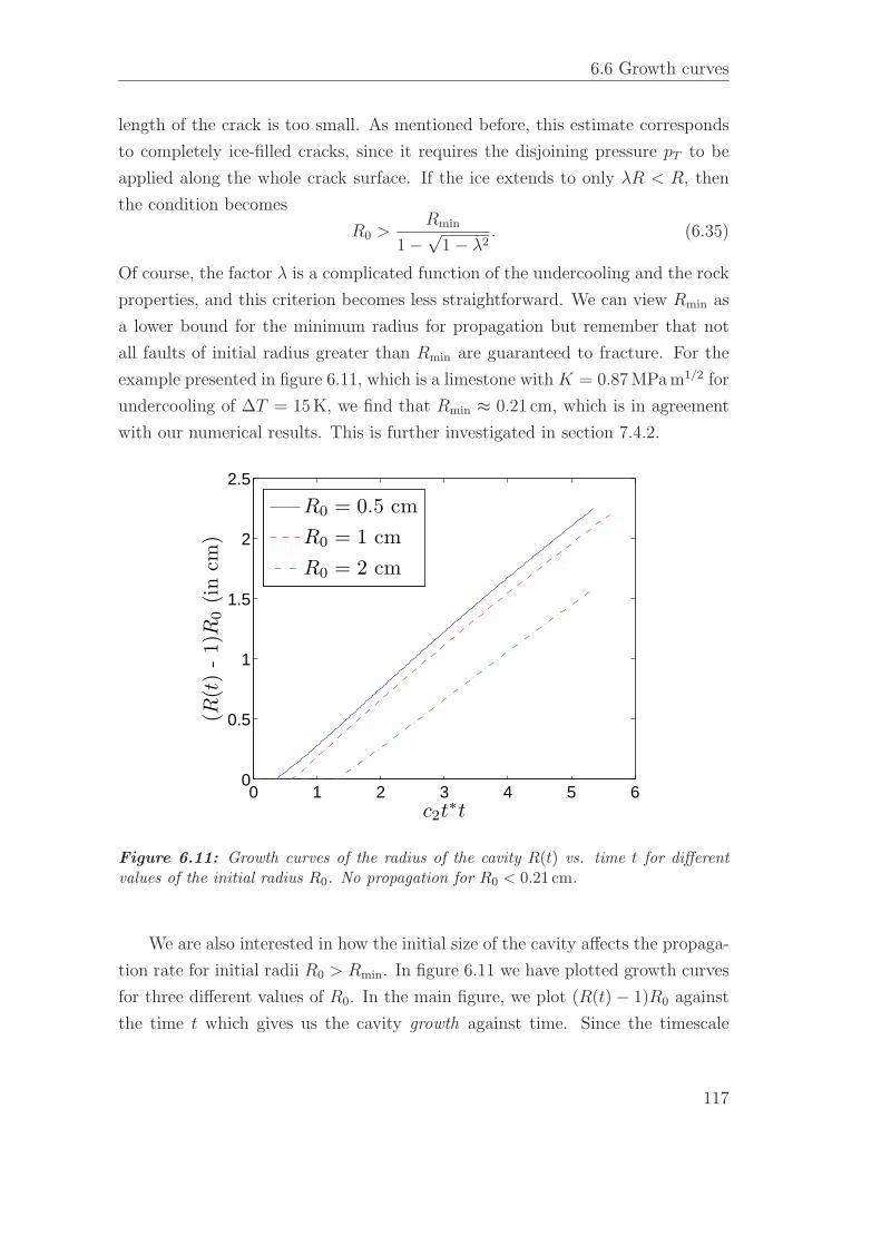
6.6 Growth curves
length of the crack is too small. As mentioned before, this estimate corresponds
to completely ice-filled cracks, since it requires the disjoining pressure pT to be
applied along the whole crack surface. If the ice extends to only λR < R, then
the condition becomes
R0 >Rmin
1 −√
1 − λ2. (6.35)
Of course, the factor λ is a complicated function of the undercooling and the rock
properties, and this criterion becomes less straightforward. We can view Rmin as
a lower bound for the minimum radius for propagation but remember that not
all faults of initial radius greater than Rmin are guaranteed to fracture. For the
example presented in figure 6.11, which is a limestone with K = 0.87 MPa m1/2 for
undercooling of ∆T = 15 K, we find that Rmin ≈ 0.21 cm, which is in agreement
with our numerical results. This is further investigated in section 7.4.2.
0 1 2 3 4 5 60
0.5
1
1.5
2
2.5
c2t∗t
(R(t
)-
1)R
0(i
ncm
)
R0 = 0.5 cm
R0 = 1 cm
R0 = 2 cm
Figure 6.11: Growth curves of the radius of the cavity R(t) vs. time t for differentvalues of the initial radius R0. No propagation for R0 < 0.21 cm.
We are also interested in how the initial size of the cavity affects the propaga-
tion rate for initial radii R0 > Rmin. In figure 6.11 we have plotted growth curves
for three different values of R0. In the main figure, we plot (R(t) − 1)R0 against
the time t which gives us the cavity growth against time. Since the timescale
117
6 Time-dependent problem
t∗ ∼ R20, we need to account for its dependence on the initial radius. We do
that by plotting against the real time t∗t, multiplied by c2 = π2Π16γ2mµ
(ρsL∆T
Tm
)4
to
keep it dimensionless. We see that, the smaller the initial radius, the less time it
takes for the critical stress condition to be reached and the propagation to start.
This does not contradict the Rmin conclusions above; the maximum pressure in
a cavity is reached faster when the cavity is smaller as less freezing is required.
If R0 < Rmin, the tip stress caused by this maximum pressure is not enough to
fracture the cavity. For R0 > Rmin, the propagation will occur as soon as KI = K.
0 2 4 6 80.5
1
1.5
2
2.5
3
3.5
4
c2t∗t
RR
0(i
ncm
)
R0 = 0.5cm
R0 = 1cm
R0 = 2cm
Figure 6.12: Growth curves of the radius of the cavity R(t) vs. time t for differentvalues of the initial radius R0. No propagation for R0 < 0.21 cm. Note that the timeorigin has been shifted between the curves.
Comparing the three different growth curves we see that their slopes are very
similar. We investigate this further by plotting the actual crack half radius R(t)R0
against the time t in figure 6.12. Like in figure 6.12, we plot the radius against
c2t∗t to take into account the dependence of the timescale on R0. The curves for
R0 = 1 cm and R0 = 2 cm are shifted in time to match the R0 = 0.5 cm curve at
R0R(t) = 1 cm and R0R(t) = 2 cm respectively. It is interesting that the three
curves appear now to completely coincide. This tells us that the propagation rate
at any time is only dependent on the cavity radius at that time and not on the
118
6.6 Growth curves
initial radius R0. Hence, a crack that started from an R0-sized fault and one
that started from a 2R0-sized fault will propagate in an almost identical way if
we ignore the initial time it takes for the smaller cavity to reach R(t) = 2R0.
This important conclusion means that the initial condition we use only has an
important effect on the fracturing potential of the crack rather than the rate of
fracturing.
6.6.4 Growth characteristics
The rate of fracturing of the cavity depends on several parameters of the prob-
lem, a few of which we investigated in sections 6.6.1-6.6.3. The propagation rate
depends on both the undercooling and the fracture toughness of the medium.
A rock being prone to fracturing means that the fracture toughness K is small.
Tough rocks will require large pressures for the stress at the tip to reach the crit-
ical value K. We saw that the maximum pressure is temperature dependent as
described by equation (6.32) and that faster propagation is predicted for larger
undercoolings, as the solidification is faster.
We plot the growth curves for both a weak (small K) and a tough (large K)
rock in figures 6.13 and 6.14. We notice there is a qualitative difference between
the two: for the weak rock, propagation is fastest for early times. Meanwhile,
for the tough rock, early propagation is slow but speeds up for t > 10. This is
accompanied by a contrasting behaviour of the solid and liquid pressures ps and
pl, which are plotted, averaged over the length of the crack, on the right hand
side of figures 6.13 and 6.14.
In both cases, there is a contrasting behaviour of the absolute values of the pres-
sures: while |pl| increases with time, supplying the cavity with an increasing flux
of water, ps decreases. The latter behaviour is easily explained if we consider the
integral expression (4.16) for the stress at the tip induced by a given solid pressure
distribution: as the crack extends, the region over which the solid pressure acts is
larger. The stress-intensity factor is the integrated ps over the whole crack and,
during propagation, is equal to the fracture toughness of the material which is
a constant. As the cavity extends, the integral of the pressure over it remains
119
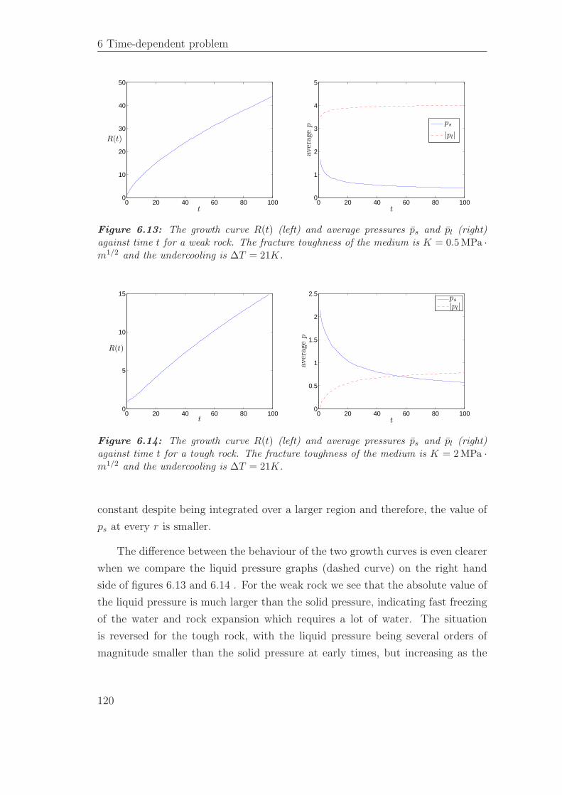
6 Time-dependent problem
0 20 40 60 80 1000
10
20
30
40
50
t
R(t)
0 20 40 60 80 1000
1
2
3
4
5
t
aver
age
p
ps
|pl|
Figure 6.13: The growth curve R(t) (left) and average pressures ps and pl (right)against time t for a weak rock. The fracture toughness of the medium is K = 0.5 MPa ·m1/2 and the undercooling is ∆T = 21K.
0 20 40 60 80 1000
5
10
15
t
R(t)
0 20 40 60 80 1000
0.5
1
1.5
2
2.5
t
aver
age
p
ps
|pl|
Figure 6.14: The growth curve R(t) (left) and average pressures ps and pl (right)against time t for a tough rock. The fracture toughness of the medium is K = 2 MPa ·m1/2 and the undercooling is ∆T = 21K.
constant despite being integrated over a larger region and therefore, the value of
ps at every r is smaller.
The difference between the behaviour of the two growth curves is even clearer
when we compare the liquid pressure graphs (dashed curve) on the right hand
side of figures 6.13 and 6.14 . For the weak rock we see that the absolute value of
the liquid pressure is much larger than the solid pressure, indicating fast freezing
of the water and rock expansion which requires a lot of water. The situation
is reversed for the tough rock, with the liquid pressure being several orders of
magnitude smaller than the solid pressure at early times, but increasing as the
120
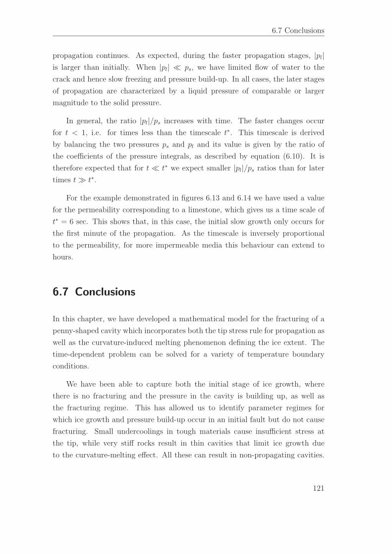
6.7 Conclusions
propagation continues. As expected, during the faster propagation stages, |pl|is larger than initially. When |pl| ≪ ps, we have limited flow of water to the
crack and hence slow freezing and pressure build-up. In all cases, the later stages
of propagation are characterized by a liquid pressure of comparable or larger
magnitude to the solid pressure.
In general, the ratio |pl|/ps increases with time. The faster changes occur
for t < 1, i.e. for times less than the timescale t∗. This timescale is derived
by balancing the two pressures ps and pl and its value is given by the ratio of
the coefficients of the pressure integrals, as described by equation (6.10). It is
therefore expected that for t ≪ t∗ we expect smaller |pl|/ps ratios than for later
times t ≫ t∗.
For the example demonstrated in figures 6.13 and 6.14 we have used a value
for the permeability corresponding to a limestone, which gives us a time scale of
t∗ = 6 sec. This shows that, in this case, the initial slow growth only occurs for
the first minute of the propagation. As the timescale is inversely proportional
to the permeability, for more impermeable media this behaviour can extend to
hours.
6.7 Conclusions
In this chapter, we have developed a mathematical model for the fracturing of a
penny-shaped cavity which incorporates both the tip stress rule for propagation as
well as the curvature-induced melting phenomenon defining the ice extent. The
time-dependent problem can be solved for a variety of temperature boundary
conditions.
We have been able to capture both the initial stage of ice growth, where
there is no fracturing and the pressure in the cavity is building up, as well as
the fracturing regime. This has allowed us to identify parameter regimes for
which ice growth and pressure build-up occur in an initial fault but do not cause
fracturing. Small undercoolings in tough materials cause insufficient stress at
the tip, while very stiff rocks result in thin cavities that limit ice growth due
to the curvature-melting effect. All these can result in non-propagating cavities.
121

6 Time-dependent problem
Assuming that the cavities are ice-filled, we have identified a lower bound for
the initial radius of a pre-existing fault which will fracture under given fracture
toughness and undercooling parameters. The expression can also be used to
determine the minimum undercooling required to fracture a cavity of a given
initial radius in a medium of a given fracture toughness.
We have also studied the effect of the different parameters of the problem on
the growth rate of the cavity. Larger undercooling or smaller fracture toughness
both result in faster fracturing. The permeability of the medium controls the flow
of water towards the solidification front. This means that it has the potential to
slow down the pressure build up and hence propagation, especially for relatively
impermeable media with permeabilities less than about 10−11 cm2.
We also find that, although the size of the initial cavity determines whether
propagation occurs or not, according to equation (6.34), it doesn’t have an effect
on the later stages of propagation. Cavities that have reached the same size after
starting from different initial radii will propagate in the same way.
The propagation characteristics were also discussed in relation to the balance
of the liquid and solid pressures. We found that, in general, low |pl| corresponds
to slow propagation and this normally occurs at the beginning of the fracturing
of a tough rock. At later times, rocks can have liquid pressures of the order of
the solid pressure.
In conclusion, the important features of crack propagation and their depen-
dence on the several parameters of the problem have been identified and analysed.
In the next chapter, we will apply the theory developed here to real-life scenarios
and compare the results with existing studies in rock fracturing.
122
Chapter 7
Applications
In the last two chapters we explored the penny-shaped crack model for differ-
ent undercooling laws. We found a similarity solution for specific undercooling
conditions and solved the more general time-dependent problem. The geome-
try we considered is applicable to several real-life situations in which media with
pre-existing faults are supercooled to some temperature from all sides. Exam-
ples include cracked pots, damaged buildings, historical monuments or statues
and many more. Even when the precise geometry is not suitable, much can be
deduced from the various scalings emerging from the modelling.
7.1 Past studies
The theoretical model for frost cracking developed by Walder & Hallet (1985) de-
scribes the propagation of an elliptical crack in a porous medium. The main con-
clusions of the study have been summarized in the introduction. Linear elasticity
123
7 Applications
was used to describe the pressure distribution, with the solid pressure uniformly
distributed on the crack walls (see also the elliptical solution from section 4.2.1).
Unlike our model, in which we assume that propagation occurs only in the
critical state KI = K, Walder & Hallet consider subcritical growth of cracks,
occurring for values of stress below the fracture toughness K. Subcritical frac-
turing can happen owing to several factors, the most usual being stress corrosion.
The stress is still required to be above a critical value, which is called the stress-
corrosion limit Ks−c. This is usually assumed to be in the region of 0.3K − 0.4K,
although difficulties in performing experiments while maintaining the stress at
such low values creates some uncertainty. Sub-critical growth is assumed to oc-
cur for a range of values of the tip stress KI > Ks−c, and not just one critical
value. Because of this, it is necessary to determine the propagation rate of the
crack caused by different stresses KI . This is usually based on results from load-
fracturing experiments, where a prescribed stress intensity KI is imposed and
the speed of the crack, V , is measured. Several equations, based on data from
experiments described above, have been proposed to describe subcritical growth.
The most used are the power law V ∼ (KI/K)n (Charles, 1958), the exponential
V ∼ eKI (Wiederhorn & Bolz, 1970), as well as V ∼ eK2I/K2
(Segall, 1984) which
is the one used by Walder & Hallet. As discussed by Atkinson (1984), because
the dependence of the crack growth rate V on the stress KI is strong, and the
data sets quite limited in range, it is difficult to distinguish between the different
models. In addition to this, it is not clear if all materials have a stress-corrosion
limit, and hence experience subcritical fracturing, as most experimental evidence
concerns glasses and there is limited data on rocks and ceramics (Freiman, 1984).
The V vs. KI law is coupled with a mass conservation of water, relating the
amount of ice freezing inside the cavity and the water flow required for it, in terms
of the hydraulic resistance of the cavity. Through that, Walder & Hallet compute
the radius of the cavity against time. In contrast to this, our model only predicts
cracking for KI = K, hence the propagation rate is directly determined by the
pressure balance across the premelted interface and does not rely on empirical
observations. Two terms contribute to the resistance to the flow into the cavity:
the permeability of the medium, and the resistance to flow from the liquid layer
of thickness h at the crack wall. The inverses of the two terms, proportional to
1/Π and 1/h3, are added to give the flow resistance factor Rf . For example, a
124
7.1 Past studies
larger permeability offers less resistance to the flow. The second term corresponds
to the spreading of the water when it exits the pores of the surrounding medium
into the liquid film inside the crack and, according to Walder & Hallet (1985),
can dominate Rf for small undercoolings (not much pore ice) or coarse grains. In
our model, we recognise that the premelted film is too thin for significant flow to
be occurring along the length of the cavity (see section 4.1.3). We assume though
that the size of the grains is small enough for the spreading of the water as it
enters the film to not present significant resistance to the flow. While this can
become significant for grain sizes of a few mm, the rocks considered here will have
considerably smaller grains. For example, one of the most coarse-grained rocks
is granite, with a grain size of 0.75 mm (Atkinson & Rawlings, 1981), but it is a
relatively impermeable rock, hence its permeability dominates the flow resistance.
More permeable media like limestones or clays are much finer-grained, resulting
in a similar balance.
So far, we have ignored the effect that the porosity φ of the medium has on
the flow of water into the cavity. In some cases though (e.g. clays), φ can be
as large as 0.4 − 0.5, and hence its effect can become important. This will be
analysed in section 7.4.1. The existence of a frozen fringe is also discussed in later
sections of this chapter.
Walder & Hallet applied their model to examples of granite and marble for
both sustained freezing and gradual cooling with a linear temperature variation
with time. The growth rates predicted are slow, of the order of mm in tens of
hours. Especially at low temperatures, their theory predicts considerable amounts
of pore ice and hence very low effective permeability which restricts the water flow
towards the solidification front. This slows down the freezing and therefore the
pressure build-up. As a result, they find that in most cases the most effective
fracturing occurs at temperatures between −5◦ C and −14◦ C, as for smaller un-
dercoolings there is not enough ice growth and pressure build-up, while at larger
undercoolings the process is significantly slowed down owing to the large amount
of pore ice restricting the water flow. This interval for “optimal fracturing” is
supported experimentally by Hallet et al. (1991), who used acoustic emissions
to detect fractures in a frozen rock. It is important to note here that, at low
temperatures, the Walder & Hallet model predicts slower fracturing, rather than
no fracturing at all. For example, the instantaneous growth rate for a crack in
125
7 Applications
granite is found (numerically) to be zero after 50 hours of freezing at −20◦ C,
but after 100 hours, fracturing is predicted. This is in agreement with our model
which predicts that fracturing of a cavity of a given size in a medium of a given
toughness will always occur for undercoolings larger than a critical value, inde-
pendent of parameters such as the permeability or the elasticity of the medium,
which can only affect the timescale. This is discussed further in section 7.4.
As we have seen in chapter 6, the timescale of our model is much smaller than
that predicted by Walder & Hallet, of the order of minutes for unfrozen granite.
We have seen that the timescale is inversely proportional to the permeability
of the medium, which indicates that the large discrepancies between ours and
Walder & Hallet’s numerical results are due to our different assumptions about
the existence of pore ice. The differences between the two models, and how they
affect the numerical results, are further discussed in section 7.2.
Murton et al. (2006) used Walder & Hallet’s model coupled with heat and wa-
ter transfer equations, given respectively by a thermal energy balance and Darcy’s
law. The pore ice content features explicitly in the energy balance equation and
appears in the effective permeability with some free parameters determined by
experimental measurements. Unlike Walder & Hallet, the sub-critical growth in
this case was modelled by V ∼ eKI/K . A year-long experiment was done on
freezing of a block of chalk. The bottom was kept at temperatures below 0◦ C,
simulating permafrost, while the upper half cycled above and below 0◦ C, simu-
lating seasonal temperature variations. Numerical results are presented for crack
length, solid pressure variations and depth at which fractures occurred, and the
latter is compared to experimental data. The undercoolings are relatively small,
which implies slow fracturing, and melting of the ice inside cracks can occur dur-
ing the thaw cycles. Their numerical predictions for the depth at which cracks
appear agree with their experimental findings when an initial distribution of 5 mm
cracks is assumed. As noted in the paper, the choice of initial crack radius has a
negligible effect on the long-time fracturing rate, which agrees with our findings
in section 6.6.3. Despite this, we would expect it to have an important role in
determining the depth at which the fractures appear, as the temperature field
varies through the depth of the rock, with the colder region being at the bottom.
As we will see in section 7.4.2, the undercooling required for a cavity to fracture
is inversely proportional to the square root of the initial radius of the cavity. This
126
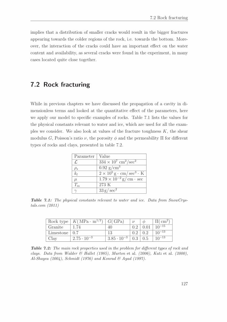
7.2 Rock fracturing
implies that a distribution of smaller cracks would result in the bigger fractures
appearing towards the colder regions of the rock, i.e. towards the bottom. More-
over, the interaction of the cracks could have an important effect on the water
content and availability, as several cracks were found in the experiment, in many
cases located quite close together.
7.2 Rock fracturing
While in previous chapters we have discussed the propagation of a cavity in di-
mensionless terms and looked at the quantitative effect of the parameters, here
we apply our model to specific examples of rocks. Table 7.1 lists the values for
the physical constants relevant to water and ice, which are used for all the exam-
ples we consider. We also look at values of the fracture toughness K, the shear
modulus G, Poisson’s ratio ν, the porosity φ and the permeability Π for different
types of rocks and clays, presented in table 7.2.
Parameter ValueL 334 × 107 cm2/sec2
ρs 0.92 g/cm3
kl 2 × 10⁵ g · cm/ sec3 · Kµ 1.79 × 10⁻² g/ cm · secTm 273 Kγ 33 g/ sec2
Table 7.1: The physical constants relevant to water and ice. Data from SnowCrys-tals.com (2011)
Rock type K( MPa · m1/2) G( GPa) ν φ Π( cm2)Granite 1.74 40 0.2 0.01 10−15
Limestone 0.7 13 0.2 0.2 10−13
Clay 2.75 · 10−3 3.85 · 10−3 0.3 0.5 10−13
Table 7.2: The main rock properties used in the problem for different types of rock andclays. Data from Walder & Hallet (1985), Murton et al. (2006), Katz et al. (2000),Al-Shayea (2004), Schmidt (1976) and Konrad & Ayad (1997).
127
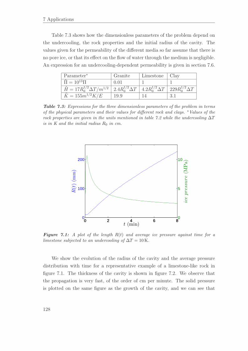
7 Applications
Table 7.3 shows how the dimensionless parameters of the problem depend on
the undercooling, the rock properties and the initial radius of the cavity. The
values given for the permeability of the different media so far assume that there is
no pore ice, or that its effect on the flow of water through the medium is negligible.
An expression for an undercooling-dependent permeability is given in section 7.6.
Parameter∗ Granite Limestone Clay
Π = 1013Π 0.01 1 1
H = 17R1/20 ∆T/m1/2 2.4R
1/20 ∆T 4.2R
1/20 ∆T 229R
1/20 ∆T
K = 155m1/2K/E 19.9 14 3.1
Table 7.3: Expressions for the three dimensionless parameters of the problem in termsof the physical parameters and their values for different rock and clays. ∗Values of therock properties are given in the units mentioned in table 7.2 while the undercooling ∆Tis in K and the initial radius R0 in cm.
0 2 4 6 80
100
200
t (min)
R(t
)(m
m)
0 2 4 6 80
5
10
ice
pre
ssure
(MPa)
Figure 7.1: A plot of the length R(t) and average ice pressure against time for alimestone subjected to an undercooling of ∆T = 10 K.
We show the evolution of the radius of the cavity and the average pressure
distribution with time for a representative example of a limestone-like rock in
figure 7.1. The thickness of the cavity is shown in figure 7.2. We observe that
the propagation is very fast, of the order of cm per minute. The solid pressure
is plotted on the same figure as the growth of the cavity, and we can see that
128
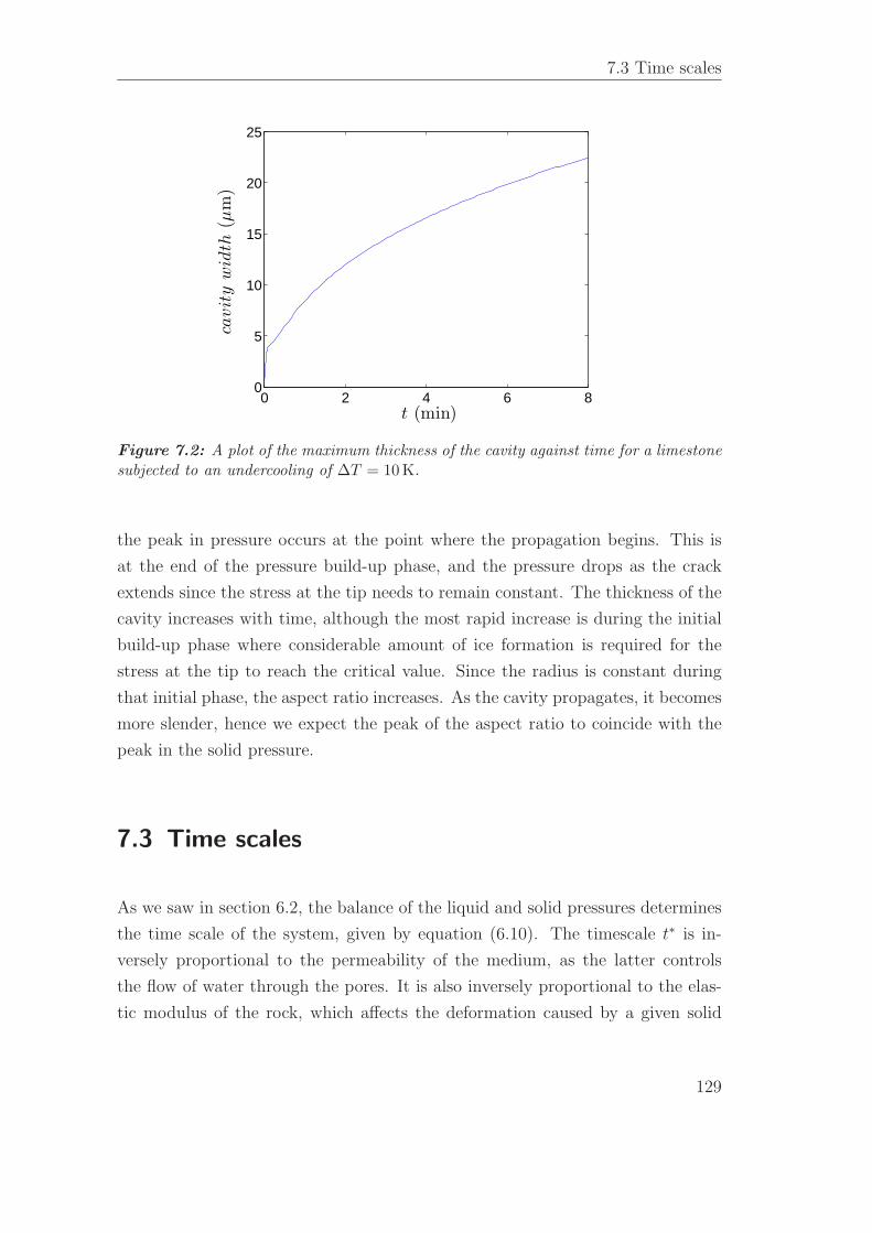
7.3 Time scales
0 2 4 6 80
5
10
15
20
25
t (min)
cavit
yw
idth
(µm
)
Figure 7.2: A plot of the maximum thickness of the cavity against time for a limestonesubjected to an undercooling of ∆T = 10 K.
the peak in pressure occurs at the point where the propagation begins. This is
at the end of the pressure build-up phase, and the pressure drops as the crack
extends since the stress at the tip needs to remain constant. The thickness of the
cavity increases with time, although the most rapid increase is during the initial
build-up phase where considerable amount of ice formation is required for the
stress at the tip to reach the critical value. Since the radius is constant during
that initial phase, the aspect ratio increases. As the cavity propagates, it becomes
more slender, hence we expect the peak of the aspect ratio to coincide with the
peak in the solid pressure.
7.3 Time scales
As we saw in section 6.2, the balance of the liquid and solid pressures determines
the time scale of the system, given by equation (6.10). The timescale t∗ is in-
versely proportional to the permeability of the medium, as the latter controls
the flow of water through the pores. It is also inversely proportional to the elas-
tic modulus of the rock, which affects the deformation caused by a given solid
129
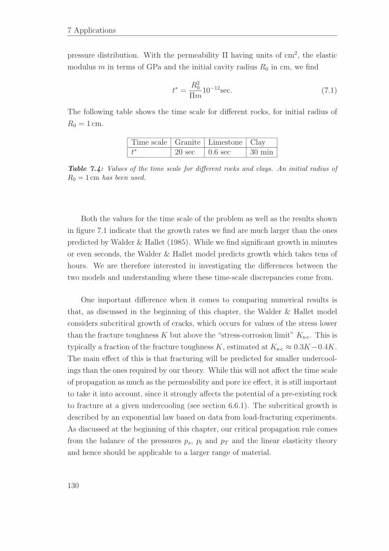
7 Applications
pressure distribution. With the permeability Π having units of cm2, the elastic
modulus m in terms of GPa and the initial cavity radius R0 in cm, we find
t∗ =R2
0
Πm10−12sec. (7.1)
The following table shows the time scale for different rocks, for initial radius of
R0 = 1 cm.
Time scale Granite Limestone Clayt∗ 20 sec 0.6 sec 30 min
Table 7.4: Values of the time scale for different rocks and clays. An initial radius ofR0 = 1 cm has been used.
Both the values for the time scale of the problem as well as the results shown
in figure 7.1 indicate that the growth rates we find are much larger than the ones
predicted by Walder & Hallet (1985). While we find significant growth in minutes
or even seconds, the Walder & Hallet model predicts growth which takes tens of
hours. We are therefore interested in investigating the differences between the
two models and understanding where these time-scale discrepancies come from.
One important difference when it comes to comparing numerical results is
that, as discussed in the beginning of this chapter, the Walder & Hallet model
considers subcritical growth of cracks, which occurs for values of the stress lower
than the fracture toughness K but above the “stress-corrosion limit” Ks-c. This is
typically a fraction of the fracture toughness K, estimated at Ks-c ≈ 0.3K−0.4K.
The main effect of this is that fracturing will be predicted for smaller undercool-
ings than the ones required by our theory. While this will not affect the time scale
of propagation as much as the permeability and pore ice effect, it is still important
to take it into account, since it strongly affects the potential of a pre-existing rock
to fracture at a given undercooling (see section 6.6.1). The subcritical growth is
described by an exponential law based on data from load-fracturing experiments.
As discussed at the beginning of this chapter, our critical propagation rule comes
from the balance of the pressures ps, pl and pT and the linear elasticity theory
and hence should be applicable to a larger range of material.
130

7.3 Time scales
Furthermore, Walder & Hallet apply their model to relatively impermeable
rocks and include the effect of a frozen fringe. It is important to point out
here that since they are considering a frozen fringe, the effective permeability of
the medium is significantly smaller than it would be in the absence of pore ice.
The contribution to the “flow resistance” Rf from the frozen fringe alone makes
for a rather large flow resistance, with the effective permeability at just 1◦C of
undercooling being of the order of 10−16cm2 (value derived from their data for the
hydraulic conductivity of the medium), and inversely proportional to the squared
power of the undercooling.
0 20 40 60 80 100 12050
55
60
65
70
t (h)
R(t
)(m
m)
W &H results
our results
Figure 7.3: Crack growth vs. time for a cavity of initial radius R0 = 50 mm in granite,with undercooling of 6 ◦C. The red squares represent numerical results from Walder &Hallet.
With these differences taken into account, we can attempt a direct comparison
of their numerical results with our theory. With the adjusted values for effective
permeability due to pore ice, we find propagation rates much closer to those
predicted by Walder & Hallet. Figures 7.3 and 7.4 show the evolution of the
radius R(t) and solid pressure ps with time. We see that the agreement of the
initial time it takes for the propagation to begin is good, and the peaks in the
solid pressure are also in agreement. During the propagating phase, the Walder
& Hallet model predicts slightly faster growth than ours. The difference in the
pressure curves is consistent with the growth curves, as faster propagation means
131
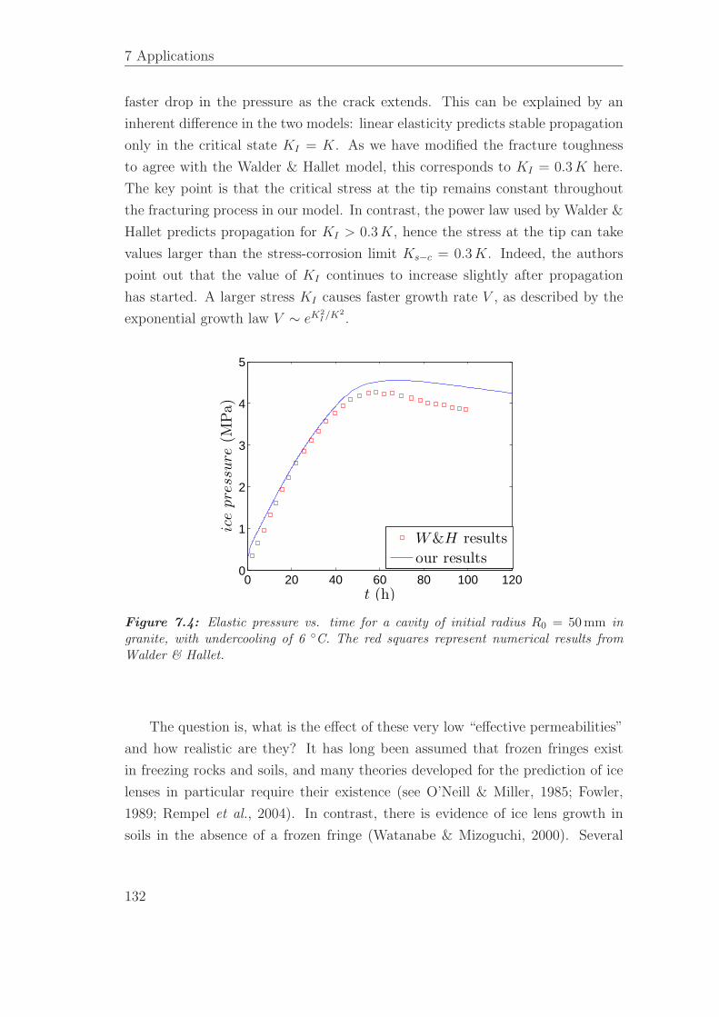
7 Applications
faster drop in the pressure as the crack extends. This can be explained by an
inherent difference in the two models: linear elasticity predicts stable propagation
only in the critical state KI = K. As we have modified the fracture toughness
to agree with the Walder & Hallet model, this corresponds to KI = 0.3 K here.
The key point is that the critical stress at the tip remains constant throughout
the fracturing process in our model. In contrast, the power law used by Walder &
Hallet predicts propagation for KI > 0.3 K, hence the stress at the tip can take
values larger than the stress-corrosion limit Ks−c = 0.3 K. Indeed, the authors
point out that the value of KI continues to increase slightly after propagation
has started. A larger stress KI causes faster growth rate V , as described by the
exponential growth law V ∼ eK2I/K2
.
0 20 40 60 80 100 1200
1
2
3
4
5
t (h)
ice
pre
ssure
(MPa)
W&H results
our results
Figure 7.4: Elastic pressure vs. time for a cavity of initial radius R0 = 50 mm ingranite, with undercooling of 6 ◦C. The red squares represent numerical results fromWalder & Hallet.
The question is, what is the effect of these very low “effective permeabilities”
and how realistic are they? It has long been assumed that frozen fringes exist
in freezing rocks and soils, and many theories developed for the prediction of ice
lenses in particular require their existence (see O’Neill & Miller, 1985; Fowler,
1989; Rempel et al., 2004). In contrast, there is evidence of ice lens growth in
soils in the absence of a frozen fringe (Watanabe & Mizoguchi, 2000). Several
132
7.3 Time scales
factors (curvature melting, premelting etc.) contribute towards the lowering of
the freezing temperature inside small pores, so all of them have to be taken
into account when predicting the existence of pore ice. While it is relatively
easy to predict if ice can exist in a pore of a certain size (see appendix E), it
is less straightforward to quantify the effect that the pore ice has on the overall
permeability of the medium. This is discussed in more details in section 7.6. Our
model shows that a frozen fringe is not necessary for frost fracturing. It also allows
us to consider whether the existence of pore ice can lower the effective permeability
enough to make expansion effects important, as was seen in chapter 3. At the end
of section 3.2 it was shown that the expansion effect becomes important when
x ∼ 1015Π cm−2, (7.2)
i.e. for large radii (x ≈ 1) and small permeabilities (Π < 10−15 cm2). For a
penny-shaped cavity, it is more complicated to quantify the expansion regime
pressure, as the growth of the ice will be asymmetric. We can estimate though
that the worst case scenario will again occur when x ≈ 1, which corresponds to
the case where a large part of the pre-existing fault is occupied with ice which
is growing, but no considerable deformation of the cavity has occurred yet. The
values of permeability for which the expansion can produce large pressures are
not unreasonable for some of the frozen granites Walder & Hallet are considering.
Even though this phenomenon is sensitive to the saturation of the medium as well
as the exact process of ice growth at the early stages of solidification, we expect
that in some cases, high pressures can develop not only during the premelting
stage, where the pre-existing faults are ice-filled, but also during the initial stage
of freezing.
Finally, it is important to note that, despite the two different sets of results not
completely overlapping, our method can reproduce the qualitative features of the
Walder & Hallet model, when we adjust the permeability and fracture toughness
so that they reflect some of their assumptions. We note that the initially slow
and then rapidly accelerating fracturing can be seen in both models. As discussed
at the beginning of this chapter, the empirical law used by Walder & Hallet
is not the only one that can be used to describe subcritical fracturing. Most
laboratory experiments provide data of a small range, making it impossible to
distinguish between the different laws discussed at the beginning of section 7.1.
133
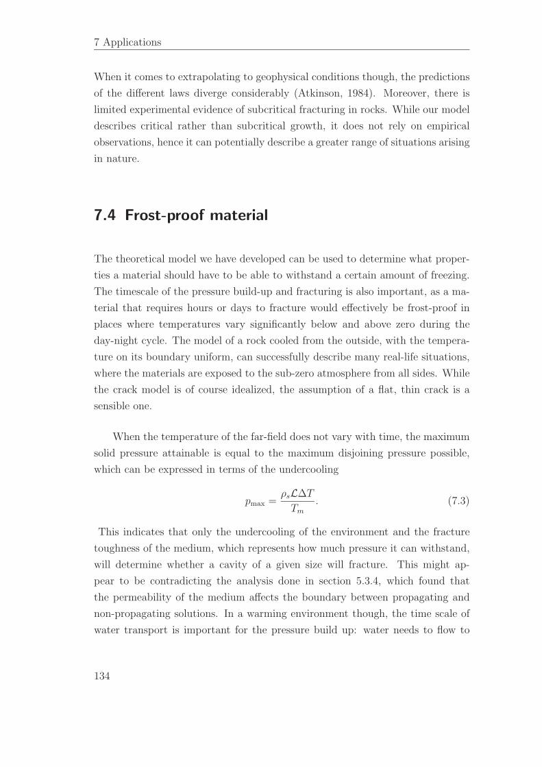
7 Applications
When it comes to extrapolating to geophysical conditions though, the predictions
of the different laws diverge considerably (Atkinson, 1984). Moreover, there is
limited experimental evidence of subcritical fracturing in rocks. While our model
describes critical rather than subcritical growth, it does not rely on empirical
observations, hence it can potentially describe a greater range of situations arising
in nature.
7.4 Frost-proof material
The theoretical model we have developed can be used to determine what proper-
ties a material should have to be able to withstand a certain amount of freezing.
The timescale of the pressure build-up and fracturing is also important, as a ma-
terial that requires hours or days to fracture would effectively be frost-proof in
places where temperatures vary significantly below and above zero during the
day-night cycle. The model of a rock cooled from the outside, with the tempera-
ture on its boundary uniform, can successfully describe many real-life situations,
where the materials are exposed to the sub-zero atmosphere from all sides. While
the crack model is of course idealized, the assumption of a flat, thin crack is a
sensible one.
When the temperature of the far-field does not vary with time, the maximum
solid pressure attainable is equal to the maximum disjoining pressure possible,
which can be expressed in terms of the undercooling
pmax =ρsL∆T
Tm
. (7.3)
This indicates that only the undercooling of the environment and the fracture
toughness of the medium, which represents how much pressure it can withstand,
will determine whether a cavity of a given size will fracture. This might ap-
pear to be contradicting the analysis done in section 5.3.4, which found that
the permeability of the medium affects the boundary between propagating and
non-propagating solutions. In a warming environment though, the time scale of
water transport is important for the pressure build up: water needs to flow to
134
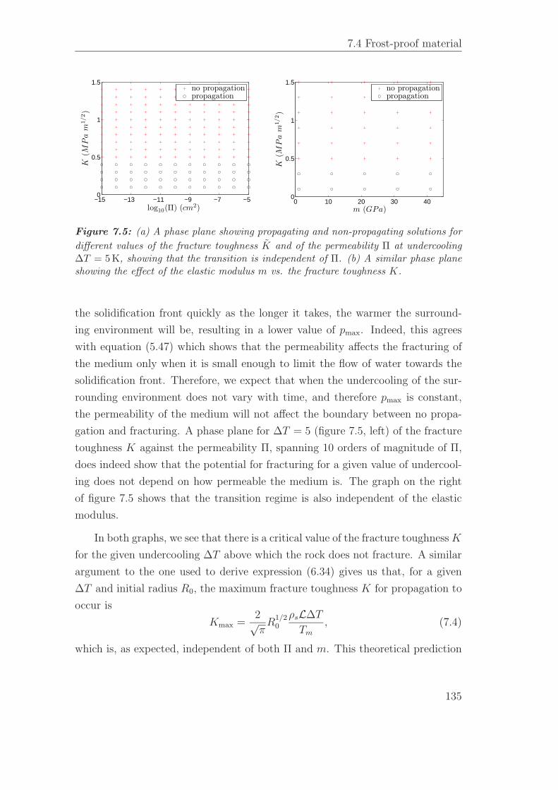
7.4 Frost-proof material
−15 −13 −11 −9 −7 −50
0.5
1
1.5
log10(Π) (cm2)
K(M
Pa
m1/2)
no propagationpropagation
0 10 20 30 400
0.5
1
1.5
m (GPa)
K(M
Pa
m1/2)
no propagationpropagation
Figure 7.5: (a) A phase plane showing propagating and non-propagating solutions for
different values of the fracture toughness K and of the permeability Π at undercooling∆T = 5 K, showing that the transition is independent of Π. (b) A similar phase planeshowing the effect of the elastic modulus m vs. the fracture toughness K.
the solidification front quickly as the longer it takes, the warmer the surround-
ing environment will be, resulting in a lower value of pmax. Indeed, this agrees
with equation (5.47) which shows that the permeability affects the fracturing of
the medium only when it is small enough to limit the flow of water towards the
solidification front. Therefore, we expect that when the undercooling of the sur-
rounding environment does not vary with time, and therefore pmax is constant,
the permeability of the medium will not affect the boundary between no propa-
gation and fracturing. A phase plane for ∆T = 5 (figure 7.5, left) of the fracture
toughness K against the permeability Π, spanning 10 orders of magnitude of Π,
does indeed show that the potential for fracturing for a given value of undercool-
ing does not depend on how permeable the medium is. The graph on the right
of figure 7.5 shows that the transition regime is also independent of the elastic
modulus.
In both graphs, we see that there is a critical value of the fracture toughness K
for the given undercooling ∆T above which the rock does not fracture. A similar
argument to the one used to derive expression (6.34) gives us that, for a given
∆T and initial radius R0, the maximum fracture toughness K for propagation to
occur is
Kmax =2√π
R1/20
ρsL∆T
Tm
, (7.4)
which is, as expected, independent of both Π and m. This theoretical prediction
135
7 Applications
0 5 10 150
0.5
1
1.5
∆T (K)
K(M
Pa
m1/2)
no propagation
propagation
analytic prediction
Figure 7.6: A phase plane showing propagating and non-propagating solutions for
different values of the fracture toughness K and of the undercooling ∆T . The green lineshows the theoretical prediction defined by equation (7.4).
can be seen in figure 7.6, where we have plotted the slope between K and ∆T
(green line). We see that the match is not perfect, which is a result of the cavity
not being completely ice-filled, as was explained in section 5.3.2. The quantitative
effect of λ < 1 on the above expression is described by equation (6.35).
From the above we can conclude that the most important parameters for the
susceptibility of a medium to fracturing are the fracture toughness of the material
and the undercooling of the environment. The size of the pre-existing faults also
strongly influences the fracturing potential, as indicated by equation (7.4). We
will discuss this further in section 7.4.2. We also found that the permeability and
elasticity of the medium do not affect the potential for fracturing in the idealized
situation of constant undercooling but have an important effect on the timescale
of propagation, as we will see in section 7.5. In real situations, the tempera-
ture of the far field can vary significantly with time. As we saw in chapter 5,
both the permeability and the elasticity of the material affect the potential for
fracturing in a warming environment. In these cases, the timescale of pressure
build-up becomes important when discussing the susceptibility of a material, as
the conditions change with time.
136
7.4 Frost-proof material
7.4.1 Effect of porosity
When we derived the equations describing the flow of water through the medium
and inside the crack in section 4.1.3, we ignored the porosity of the medium
and approximated the volume outside the cavity as consisting of only rock when
using mass conservation arguments. Considering the flow of water into the porous
medium, we only included the component of the Darcy flow u as the contribution
to the flux at the film–rock boundary z = b. In reality, a proportion φ of the rock
is already occupied with water and hence, as the rock boundary deforms with
velocity ∂b∂t
, an additional term of −φ∂b∂t
needs to be included in the contribution
of the flux at z = b. This indicates that in the frame of reference of the thin film,
there is a component of the flow out of the cavity, acting in an opposing way
to the Darcy flow. This makes sense physically; the term u expresses the flux of
the water that flows towards the cavity to fill the opening gap which is created
because areas previously occupied by rock need to be filled by water. In the limit
of φ → 1, i.e. if the rock is very porous and consists mostly of water, the effect
of the opening of the cavity is negligible, as very little space is occupied by the
rock. In the opposite limit of φ → 0, we assume most of the cavity boundary is
occupied by rock, which when it opens up frees the space to be filled by water.
This limiting case represents the assumption we made when ignoring the porosity.
The mass continuity equation in the thin film now gives
(1 − φ)∂b
∂t+
1
r
∂
∂r
(
rh3
12µ
∂pl
∂r
)
= −u(b) =Π
µ
∂p
∂z
∣∣∣z=b
. (7.5)
The factor (1 − φ) now multiplies the liquid pressure integral, giving
pl(r, t) =2
π
µ
Π(1 − φ)
∫ R(t)
0
K
(2√
rs
r + s
)∂b
∂t
s ds
s + rif r ≤ λR, (7.6)
hence it can be absorbed in Π to give a new permeability
Πφ =Π
1 − φ. (7.7)
As we have seen, a change in the permeability of the medium does not affect the
fracturing potential of a cavity but just the timescale of the pressure build-up
and subsequent fracturing. Similarly, the effect of the porosity is simply limited
137
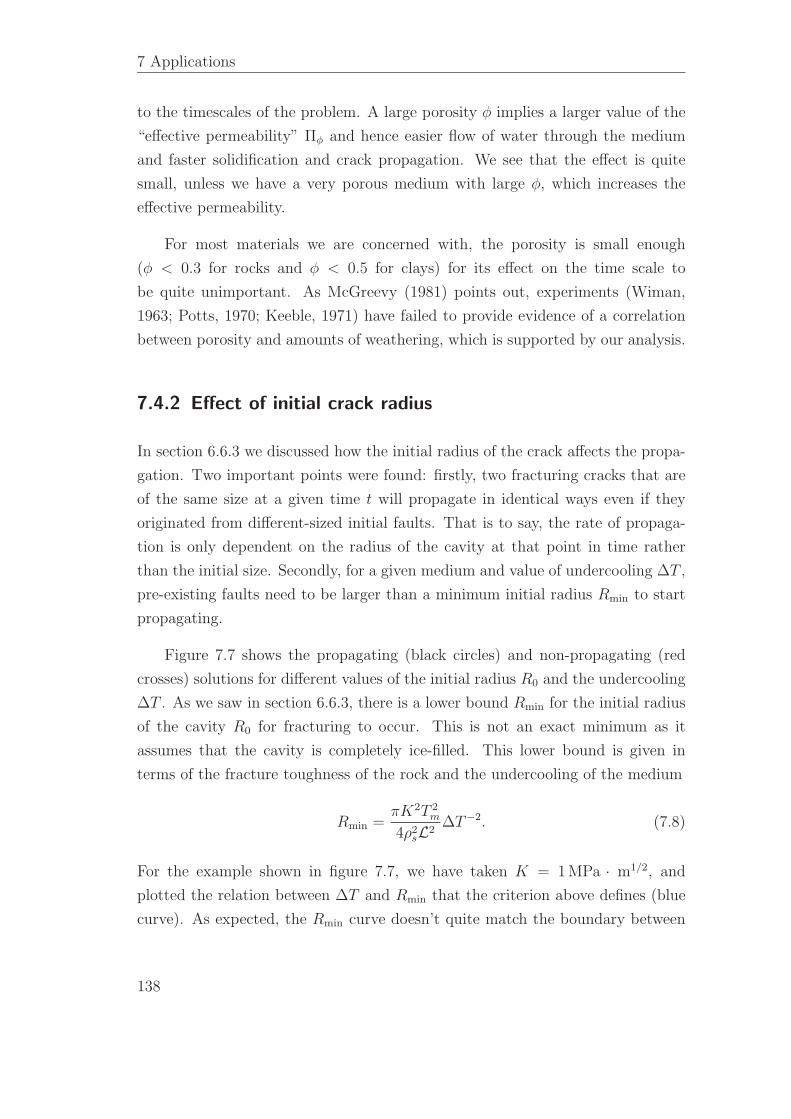
7 Applications
to the timescales of the problem. A large porosity φ implies a larger value of the
“effective permeability” Πφ and hence easier flow of water through the medium
and faster solidification and crack propagation. We see that the effect is quite
small, unless we have a very porous medium with large φ, which increases the
effective permeability.
For most materials we are concerned with, the porosity is small enough
(φ < 0.3 for rocks and φ < 0.5 for clays) for its effect on the time scale to
be quite unimportant. As McGreevy (1981) points out, experiments (Wiman,
1963; Potts, 1970; Keeble, 1971) have failed to provide evidence of a correlation
between porosity and amounts of weathering, which is supported by our analysis.
7.4.2 Effect of initial crack radius
In section 6.6.3 we discussed how the initial radius of the crack affects the propa-
gation. Two important points were found: firstly, two fracturing cracks that are
of the same size at a given time t will propagate in identical ways even if they
originated from different-sized initial faults. That is to say, the rate of propaga-
tion is only dependent on the radius of the cavity at that point in time rather
than the initial size. Secondly, for a given medium and value of undercooling ∆T ,
pre-existing faults need to be larger than a minimum initial radius Rmin to start
propagating.
Figure 7.7 shows the propagating (black circles) and non-propagating (red
crosses) solutions for different values of the initial radius R0 and the undercooling
∆T . As we saw in section 6.6.3, there is a lower bound Rmin for the initial radius
of the cavity R0 for fracturing to occur. This is not an exact minimum as it
assumes that the cavity is completely ice-filled. This lower bound is given in
terms of the fracture toughness of the rock and the undercooling of the medium
Rmin =πK2T 2
m
4ρ2sL2
∆T−2. (7.8)
For the example shown in figure 7.7, we have taken K = 1 MPa · m1/2, and
plotted the relation between ∆T and Rmin that the criterion above defines (blue
curve). As expected, the Rmin curve doesn’t quite match the boundary between
138
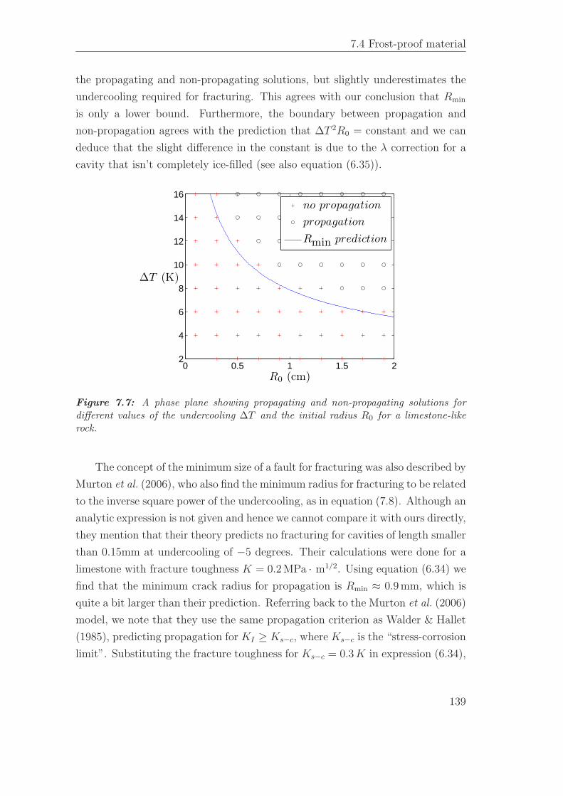
7.4 Frost-proof material
the propagating and non-propagating solutions, but slightly underestimates the
undercooling required for fracturing. This agrees with our conclusion that Rmin
is only a lower bound. Furthermore, the boundary between propagation and
non-propagation agrees with the prediction that ∆T 2R0 = constant and we can
deduce that the slight difference in the constant is due to the λ correction for a
cavity that isn’t completely ice-filled (see also equation (6.35)).
0 0.5 1 1.5 22
4
6
8
10
12
14
16
R0 (cm)
∆T (K)
no propagation
propagation
Rmin prediction
Figure 7.7: A phase plane showing propagating and non-propagating solutions fordifferent values of the undercooling ∆T and the initial radius R0 for a limestone-likerock.
The concept of the minimum size of a fault for fracturing was also described by
Murton et al. (2006), who also find the minimum radius for fracturing to be related
to the inverse square power of the undercooling, as in equation (7.8). Although an
analytic expression is not given and hence we cannot compare it with ours directly,
they mention that their theory predicts no fracturing for cavities of length smaller
than 0.15mm at undercooling of −5 degrees. Their calculations were done for a
limestone with fracture toughness K = 0.2 MPa · m1/2. Using equation (6.34) we
find that the minimum crack radius for propagation is Rmin ≈ 0.9 mm, which is
quite a bit larger than their prediction. Referring back to the Murton et al. (2006)
model, we note that they use the same propagation criterion as Walder & Hallet
(1985), predicting propagation for KI ≥ Ks−c, where Ks−c is the “stress-corrosion
limit”. Substituting the fracture toughness for Ks−c = 0.3 K in expression (6.34),
139
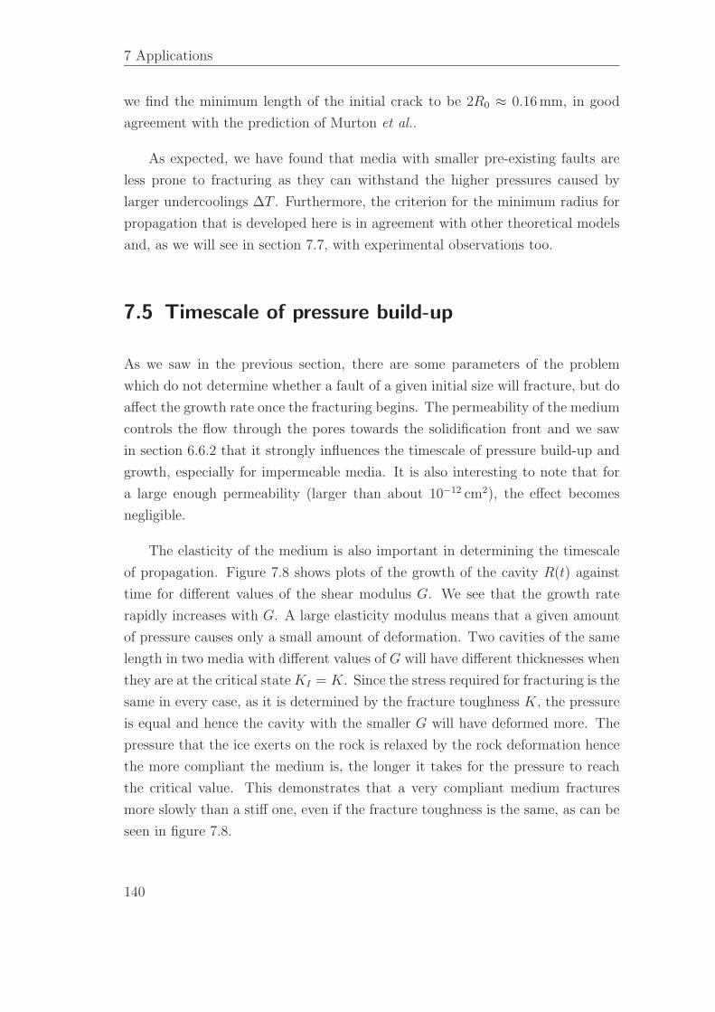
7 Applications
we find the minimum length of the initial crack to be 2R0 ≈ 0.16 mm, in good
agreement with the prediction of Murton et al..
As expected, we have found that media with smaller pre-existing faults are
less prone to fracturing as they can withstand the higher pressures caused by
larger undercoolings ∆T . Furthermore, the criterion for the minimum radius for
propagation that is developed here is in agreement with other theoretical models
and, as we will see in section 7.7, with experimental observations too.
7.5 Timescale of pressure build-up
As we saw in the previous section, there are some parameters of the problem
which do not determine whether a fault of a given initial size will fracture, but do
affect the growth rate once the fracturing begins. The permeability of the medium
controls the flow through the pores towards the solidification front and we saw
in section 6.6.2 that it strongly influences the timescale of pressure build-up and
growth, especially for impermeable media. It is also interesting to note that for
a large enough permeability (larger than about 10−12 cm2), the effect becomes
negligible.
The elasticity of the medium is also important in determining the timescale
of propagation. Figure 7.8 shows plots of the growth of the cavity R(t) against
time for different values of the shear modulus G. We see that the growth rate
rapidly increases with G. A large elasticity modulus means that a given amount
of pressure causes only a small amount of deformation. Two cavities of the same
length in two media with different values of G will have different thicknesses when
they are at the critical state KI = K. Since the stress required for fracturing is the
same in every case, as it is determined by the fracture toughness K, the pressure
is equal and hence the cavity with the smaller G will have deformed more. The
pressure that the ice exerts on the rock is relaxed by the rock deformation hence
the more compliant the medium is, the longer it takes for the pressure to reach
the critical value. This demonstrates that a very compliant medium fractures
more slowly than a stiff one, even if the fracture toughness is the same, as can be
seen in figure 7.8.
140
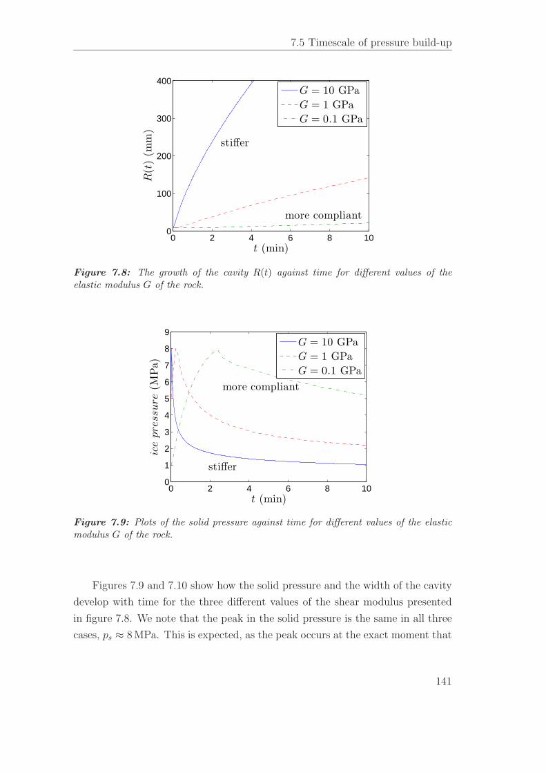
7.5 Timescale of pressure build-up
0 2 4 6 8 100
100
200
300
400
t (min)
R(t
)(m
m)
G = 10 GPa
G = 1 GPa
G = 0.1 GPa
stiffer
more compliant
Figure 7.8: The growth of the cavity R(t) against time for different values of theelastic modulus G of the rock.
0 2 4 6 8 100
1
2
3
4
5
6
7
8
9
t (min)
ice
pre
ssure
(MPa)
G = 10 GPa
G = 1 GPa
G = 0.1 GPa
stiffer
more compliant
Figure 7.9: Plots of the solid pressure against time for different values of the elasticmodulus G of the rock.
Figures 7.9 and 7.10 show how the solid pressure and the width of the cavity
develop with time for the three different values of the shear modulus presented
in figure 7.8. We note that the peak in the solid pressure is the same in all three
cases, ps ≈ 8 MPa. This is expected, as the peak occurs at the exact moment that
141
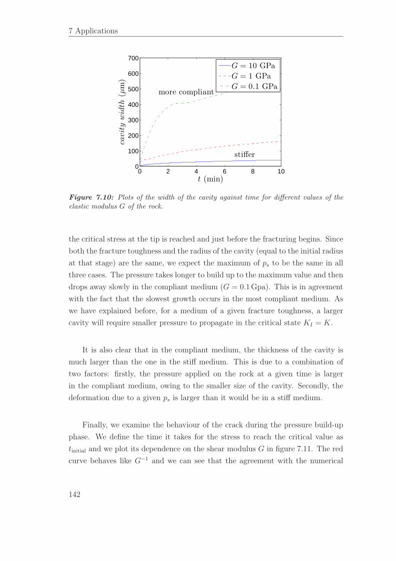
7 Applications
0 2 4 6 8 100
100
200
300
400
500
600
700
t (min)
cavit
yw
idth
(µm
)
G = 10 GPa
G = 1 GPa
G = 0.1 GPamore compliant
stiffer
Figure 7.10: Plots of the width of the cavity against time for different values of theelastic modulus G of the rock.
the critical stress at the tip is reached and just before the fracturing begins. Since
both the fracture toughness and the radius of the cavity (equal to the initial radius
at that stage) are the same, we expect the maximum of ps to be the same in all
three cases. The pressure takes longer to build up to the maximum value and then
drops away slowly in the compliant medium (G = 0.1 Gpa). This is in agreement
with the fact that the slowest growth occurs in the most compliant medium. As
we have explained before, for a medium of a given fracture toughness, a larger
cavity will require smaller pressure to propagate in the critical state KI = K.
It is also clear that in the compliant medium, the thickness of the cavity is
much larger than the one in the stiff medium. This is due to a combination of
two factors: firstly, the pressure applied on the rock at a given time is larger
in the compliant medium, owing to the smaller size of the cavity. Secondly, the
deformation due to a given ps is larger than it would be in a stiff medium.
Finally, we examine the behaviour of the crack during the pressure build-up
phase. We define the time it takes for the stress to reach the critical value as
tinitial and we plot its dependence on the shear modulus G in figure 7.11. The red
curve behaves like G−1 and we can see that the agreement with the numerical
142
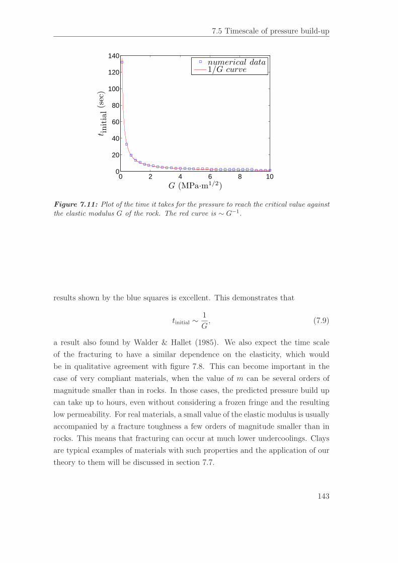
7.5 Timescale of pressure build-up
0 2 4 6 8 100
20
40
60
80
100
120
140
G (MPa·m1/2)
t init
ial(s
ec)
numerical data1/G curve
Figure 7.11: Plot of the time it takes for the pressure to reach the critical value againstthe elastic modulus G of the rock. The red curve is ∼ G−1.
results shown by the blue squares is excellent. This demonstrates that
tinitial ∼1
G, (7.9)
a result also found by Walder & Hallet (1985). We also expect the time scale
of the fracturing to have a similar dependence on the elasticity, which would
be in qualitative agreement with figure 7.8. This can become important in the
case of very compliant materials, when the value of m can be several orders of
magnitude smaller than in rocks. In those cases, the predicted pressure build up
can take up to hours, even without considering a frozen fringe and the resulting
low permeability. For real materials, a small value of the elastic modulus is usually
accompanied by a fracture toughness a few orders of magnitude smaller than in
rocks. This means that fracturing can occur at much lower undercoolings. Clays
are typical examples of materials with such properties and the application of our
theory to them will be discussed in section 7.7.
143
7 Applications
7.6 Frozen fringe
The theory developed in this thesis predicts fracturing of pre-existing faults in
rocks without the need for a frozen fringe. Previous studies of rock fracturing
(Walder & Hallet, 1985; Murton et al., 2006) have assumed the existence of pore
ice, while studies of frost heave (Rempel et al., 2004) predict no ice lens forma-
tion in the absence of a frozen fringe. Physically, when a water-saturated porous
medium is subjected to sub-zero temperatures, water inside the bigger pores can
freeze, restricting the hydraulic connectivity of the medium. The extent of the
freezing depends on the freezing-point depression, which is a result of curvature
melting or the disjoining forces between rock and ice. Quantifying this effect is dif-
ficult, as pore size varies from material to material, and there can be a large range
of pore diameters within one material too. For example, while most limestones
have pore sizes of the order of 0.1−1 µm, marbles and lithographic limestones can
have an average pore size of about 0.005µm (Lautridou & Ozouf, 1982). The crit-
ical nucleation radius for an undercooling of ∆T = 1 K is approximately 0.1 µm
and, while inversely proportional to ∆T , we see that even for low temperatures,
curvature melting can stop ice from growing inside porous material. While we
have assumed no pore ice, it is a concept that is easily incorporated into our
model. The existence of ice in the pores of a medium primarily affects the per-
meability and limits the flow of water towards the solidification front. We expect
the change in permeability to have an effect on the time scale of pressure build-up
and propagation, but not on the fracturing potential of a fault (see sections 6.6.2
and 7.4).
Both Walder & Hallet (1985) and Murton et al. (2006) consider the effect of
pore ice on the permeability of the medium. The former use a modified hydraulic
conductivity for the medium of the form k = κ1∆T−2, where the parameter κ1
is found from experimental data. The value of κ1 used in their work corresponds
to a permeability of Π = 10−16 cm2 at an undercooling of 1◦ C for a granite. In
contrast, Murton et al. include an ‘ice content’ term in the heat equation which is
then used to determine the permeability which behaves like Π ∼ (1 − I)γ , where
I is the volumetric ice fraction and γ is determined experimentally and usually
ranges between 6 and 9.
144
7.6 Frozen fringe
The permeability is closely related to the size of the pores, and can be shown
(Bear, 1988) to be proportional to the square of the average pore diameter
Π = Cd2, (7.10)
where C is a constant relating to the flow paths connecting the pores. If we
consider the growth of ice in a small spherical pore, two effects contribute to the
depression of the freezing temperature: the curvature-induced melting, and the
disjoining forces which become important when the pore is almost ice-filled, as
explained in chapter 3. It can be shown that, at first order, the smallest depression
of the freezing temperature is determined by the curvature melting effect (i.e.
dictated by the Gibbs–Thompson relation). In that case, the ice is close enough
to the rock for the curvature to be approximately given by κ = 1/d, where d is
the diameter of the pore, but not close enough for the disjoining forces to become
important, hence causing further depression of the melting temperature. The
details of the calculation are shown in appendix E.
For a given undercooling ∆T , pores that are larger than the corresponding
d∆T diameter
d∆T =γTm
ρsL∆T(7.11)
will be almost completely ice-filled, reducing the overall average pore diameter of
the medium to d < d. We expect this new average diameter d to be a function
of both the initial average pore diameter d as well as the freezing pore diameter
d∆T . When ∆T = 0, hence d∆T → ∞, no ice grows inside the pores and therefore
the average diameter remains unchanged, d = d. As the temperature drops, d∆T
becomes smaller and hence some of the pores can fill with ice. This reduces the
overall average pore size. This analysis implies a relationship between d, d and
d∆T of the form
1
d=
√
1
d2+
α
d2∆T
, (7.12)
where α is a parameter to be determined and relates to the distribution of pore
sizes of the medium. We have used the quadratic average (or root mean square)
of 1/d and 1/d∆T , rather than the mean, as this includes a measure of the spread
of the values. For example, when d∆T is large (i.e. ∆T is small) and hence 1/d∆T
is much smaller than 1/d, the quadratic average means that the effect of 1/d∆T
145
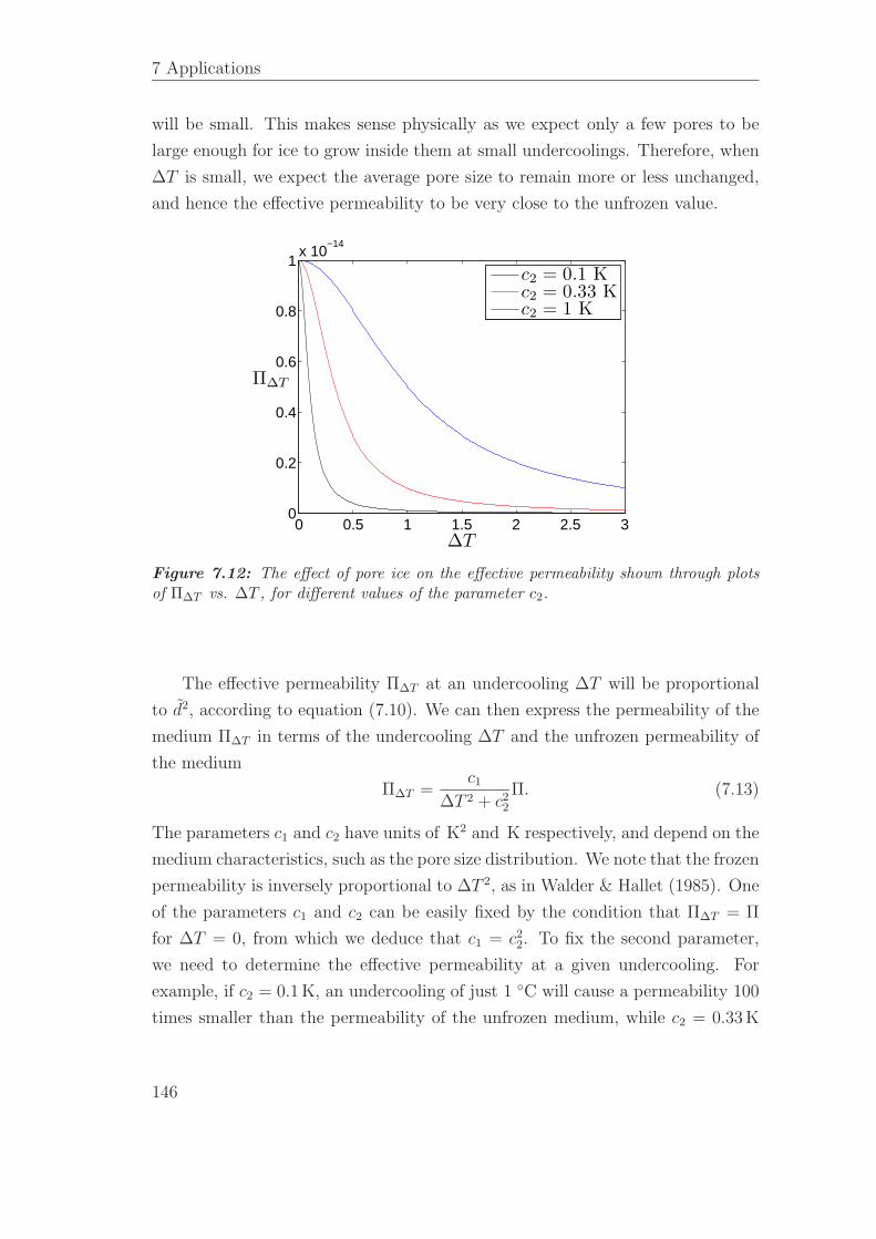
7 Applications
will be small. This makes sense physically as we expect only a few pores to be
large enough for ice to grow inside them at small undercoolings. Therefore, when
∆T is small, we expect the average pore size to remain more or less unchanged,
and hence the effective permeability to be very close to the unfrozen value.
0 0.5 1 1.5 2 2.5 30
0.2
0.4
0.6
0.8
1x 10
−14
∆T
Π∆T
c2 = 0.1 Kc2 = 0.33 Kc2 = 1 K
Figure 7.12: The effect of pore ice on the effective permeability shown through plotsof Π∆T vs. ∆T , for different values of the parameter c2.
The effective permeability Π∆T at an undercooling ∆T will be proportional
to d2, according to equation (7.10). We can then express the permeability of the
medium Π∆T in terms of the undercooling ∆T and the unfrozen permeability of
the medium
Π∆T =c1
∆T 2 + c22
Π. (7.13)
The parameters c1 and c2 have units of K2 and K respectively, and depend on the
medium characteristics, such as the pore size distribution. We note that the frozen
permeability is inversely proportional to ∆T 2, as in Walder & Hallet (1985). One
of the parameters c1 and c2 can be easily fixed by the condition that Π∆T = Π
for ∆T = 0, from which we deduce that c1 = c22. To fix the second parameter,
we need to determine the effective permeability at a given undercooling. For
example, if c2 = 0.1 K, an undercooling of just 1 ◦C will cause a permeability 100
times smaller than the permeability of the unfrozen medium, while c2 = 0.33 K
146
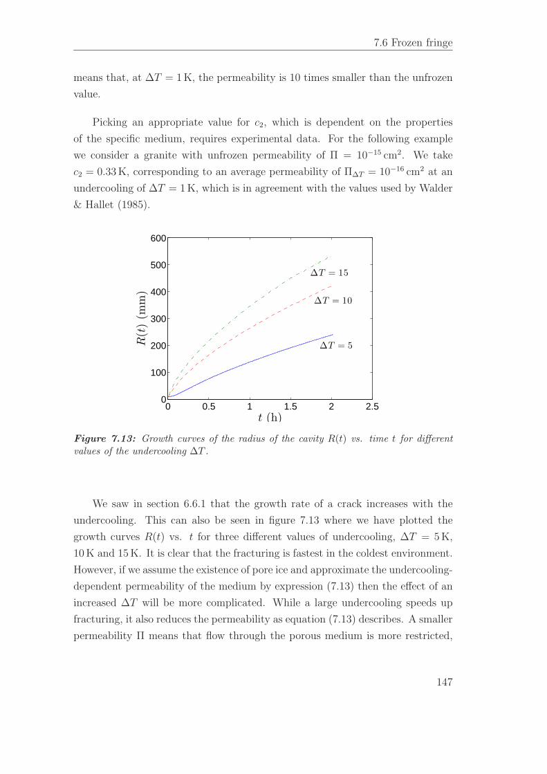
7.6 Frozen fringe
means that, at ∆T = 1 K, the permeability is 10 times smaller than the unfrozen
value.
Picking an appropriate value for c2, which is dependent on the properties
of the specific medium, requires experimental data. For the following example
we consider a granite with unfrozen permeability of Π = 10−15 cm2. We take
c2 = 0.33 K, corresponding to an average permeability of Π∆T = 10−16 cm2 at an
undercooling of ∆T = 1 K, which is in agreement with the values used by Walder
& Hallet (1985).
0 0.5 1 1.5 2 2.50
100
200
300
400
500
600
t (h)
R(t
)(m
m)
∆T = 10
∆T = 5
∆T = 15
Figure 7.13: Growth curves of the radius of the cavity R(t) vs. time t for differentvalues of the undercooling ∆T .
We saw in section 6.6.1 that the growth rate of a crack increases with the
undercooling. This can also be seen in figure 7.13 where we have plotted the
growth curves R(t) vs. t for three different values of undercooling, ∆T = 5 K,
10 K and 15 K. It is clear that the fracturing is fastest in the coldest environment.
However, if we assume the existence of pore ice and approximate the undercooling-
dependent permeability of the medium by expression (7.13) then the effect of an
increased ∆T will be more complicated. While a large undercooling speeds up
fracturing, it also reduces the permeability as equation (7.13) describes. A smaller
permeability Π means that flow through the porous medium is more restricted,
147
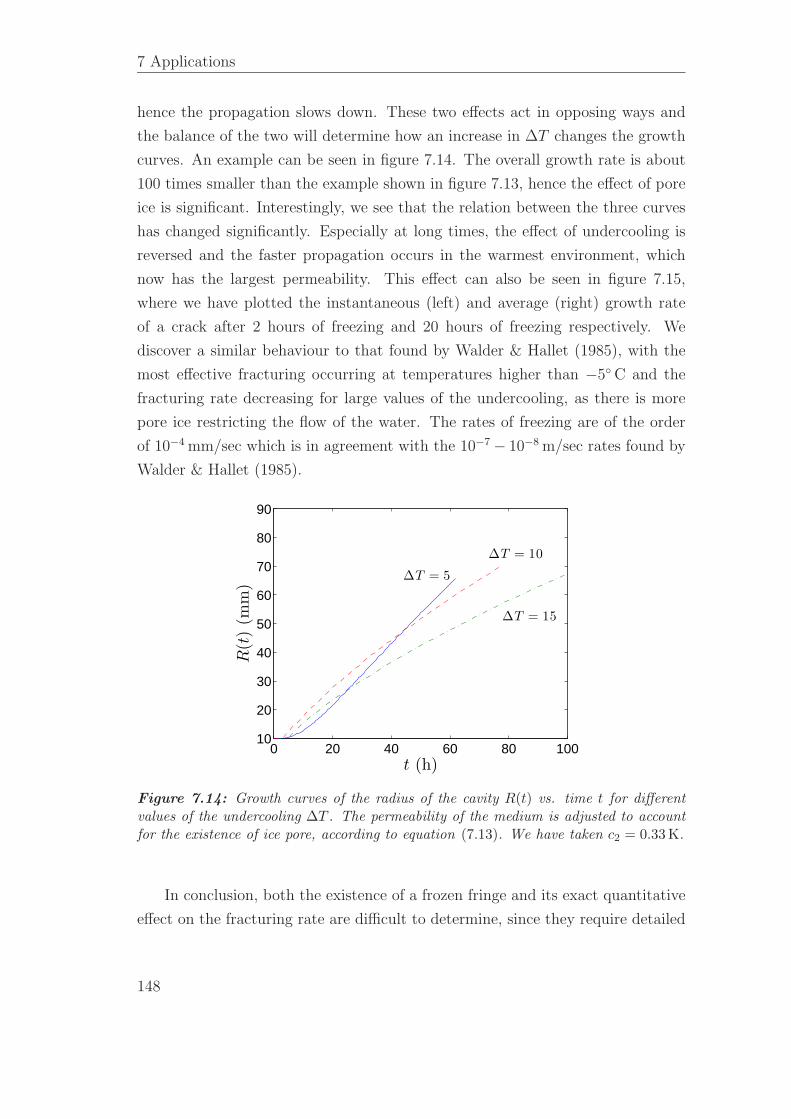
7 Applications
hence the propagation slows down. These two effects act in opposing ways and
the balance of the two will determine how an increase in ∆T changes the growth
curves. An example can be seen in figure 7.14. The overall growth rate is about
100 times smaller than the example shown in figure 7.13, hence the effect of pore
ice is significant. Interestingly, we see that the relation between the three curves
has changed significantly. Especially at long times, the effect of undercooling is
reversed and the faster propagation occurs in the warmest environment, which
now has the largest permeability. This effect can also be seen in figure 7.15,
where we have plotted the instantaneous (left) and average (right) growth rate
of a crack after 2 hours of freezing and 20 hours of freezing respectively. We
discover a similar behaviour to that found by Walder & Hallet (1985), with the
most effective fracturing occurring at temperatures higher than −5◦ C and the
fracturing rate decreasing for large values of the undercooling, as there is more
pore ice restricting the flow of the water. The rates of freezing are of the order
of 10−4 mm/sec which is in agreement with the 10−7 − 10−8 m/sec rates found by
Walder & Hallet (1985).
0 20 40 60 80 10010
20
30
40
50
60
70
80
90
t (h)
R(t
)(m
m)
∆T = 5
∆T = 10
∆T = 15
Figure 7.14: Growth curves of the radius of the cavity R(t) vs. time t for differentvalues of the undercooling ∆T . The permeability of the medium is adjusted to accountfor the existence of ice pore, according to equation (7.13). We have taken c2 = 0.33 K.
In conclusion, both the existence of a frozen fringe and its exact quantitative
effect on the fracturing rate are difficult to determine, since they require detailed
148
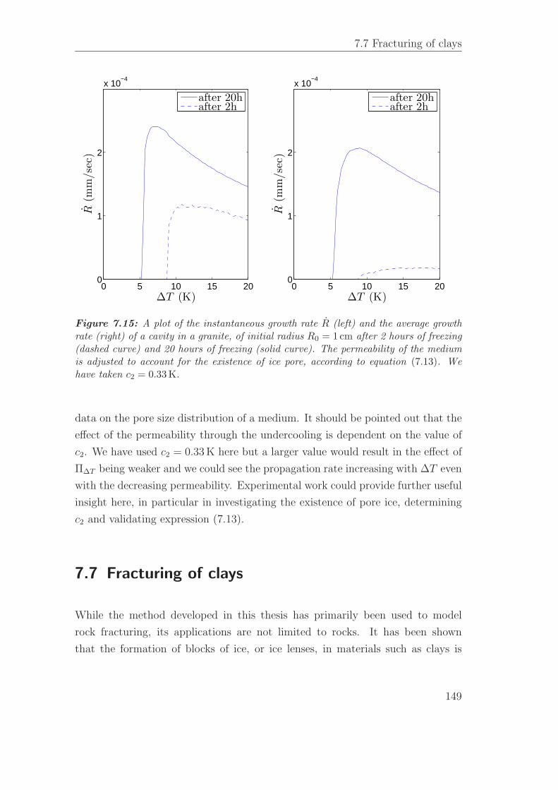
7.7 Fracturing of clays
0 5 10 15 200
1
2
x 10−4
∆T (K)
R(m
m/se
c)
after 20hafter 2h
0 5 10 15 200
1
2
x 10−4
∆T (K)
R(m
m/se
c)
after 20hafter 2h
Figure 7.15: A plot of the instantaneous growth rate R (left) and the average growthrate (right) of a cavity in a granite, of initial radius R0 = 1 cm after 2 hours of freezing(dashed curve) and 20 hours of freezing (solid curve). The permeability of the mediumis adjusted to account for the existence of ice pore, according to equation (7.13). Wehave taken c2 = 0.33 K.
data on the pore size distribution of a medium. It should be pointed out that the
effect of the permeability through the undercooling is dependent on the value of
c2. We have used c2 = 0.33 K here but a larger value would result in the effect of
Π∆T being weaker and we could see the propagation rate increasing with ∆T even
with the decreasing permeability. Experimental work could provide further useful
insight here, in particular in investigating the existence of pore ice, determining
c2 and validating expression (7.13).
7.7 Fracturing of clays
While the method developed in this thesis has primarily been used to model
rock fracturing, its applications are not limited to rocks. It has been shown
that the formation of blocks of ice, or ice lenses, in materials such as clays is
149
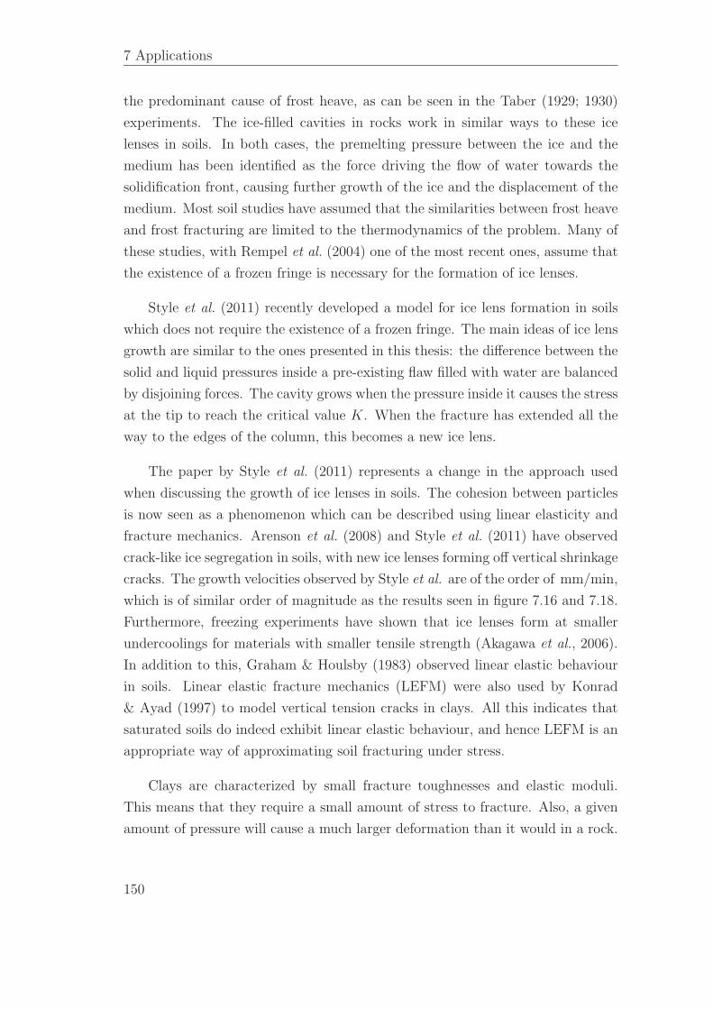
7 Applications
the predominant cause of frost heave, as can be seen in the Taber (1929; 1930)
experiments. The ice-filled cavities in rocks work in similar ways to these ice
lenses in soils. In both cases, the premelting pressure between the ice and the
medium has been identified as the force driving the flow of water towards the
solidification front, causing further growth of the ice and the displacement of the
medium. Most soil studies have assumed that the similarities between frost heave
and frost fracturing are limited to the thermodynamics of the problem. Many of
these studies, with Rempel et al. (2004) one of the most recent ones, assume that
the existence of a frozen fringe is necessary for the formation of ice lenses.
Style et al. (2011) recently developed a model for ice lens formation in soils
which does not require the existence of a frozen fringe. The main ideas of ice lens
growth are similar to the ones presented in this thesis: the difference between the
solid and liquid pressures inside a pre-existing flaw filled with water are balanced
by disjoining forces. The cavity grows when the pressure inside it causes the stress
at the tip to reach the critical value K. When the fracture has extended all the
way to the edges of the column, this becomes a new ice lens.
The paper by Style et al. (2011) represents a change in the approach used
when discussing the growth of ice lenses in soils. The cohesion between particles
is now seen as a phenomenon which can be described using linear elasticity and
fracture mechanics. Arenson et al. (2008) and Style et al. (2011) have observed
crack-like ice segregation in soils, with new ice lenses forming off vertical shrinkage
cracks. The growth velocities observed by Style et al. are of the order of mm/min,
which is of similar order of magnitude as the results seen in figure 7.16 and 7.18.
Furthermore, freezing experiments have shown that ice lenses form at smaller
undercoolings for materials with smaller tensile strength (Akagawa et al., 2006).
In addition to this, Graham & Houlsby (1983) observed linear elastic behaviour
in soils. Linear elastic fracture mechanics (LEFM) were also used by Konrad
& Ayad (1997) to model vertical tension cracks in clays. All this indicates that
saturated soils do indeed exhibit linear elastic behaviour, and hence LEFM is an
appropriate way of approximating soil fracturing under stress.
Clays are characterized by small fracture toughnesses and elastic moduli.
This means that they require a small amount of stress to fracture. Also, a given
amount of pressure will cause a much larger deformation than it would in a rock.
150
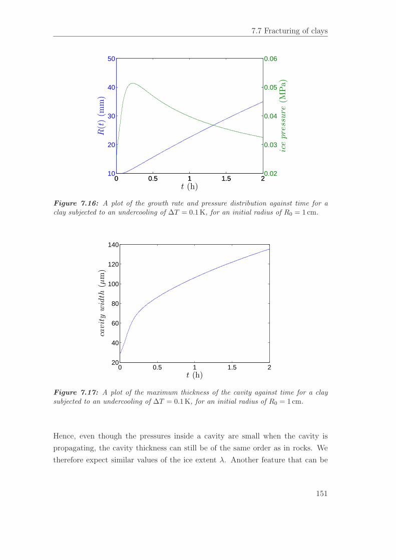
7.7 Fracturing of clays
0 0.5 1 1.5 210
20
30
40
50
R(t
)(m
m)
0 0.5 1 1.5 20.02
0.03
0.04
0.05
0.06
ice
pre
ssure
(MPa)
t (h)
Figure 7.16: A plot of the growth rate and pressure distribution against time for aclay subjected to an undercooling of ∆T = 0.1 K, for an initial radius of R0 = 1 cm.
0 0.5 1 1.5 220
40
60
80
100
120
140
t (h)
cavit
yw
idth
(µm
)
Figure 7.17: A plot of the maximum thickness of the cavity against time for a claysubjected to an undercooling of ∆T = 0.1 K, for an initial radius of R0 = 1 cm.
Hence, even though the pressures inside a cavity are small when the cavity is
propagating, the cavity thickness can still be of the same order as in rocks. We
therefore expect similar values of the ice extent λ. Another feature that can be
151
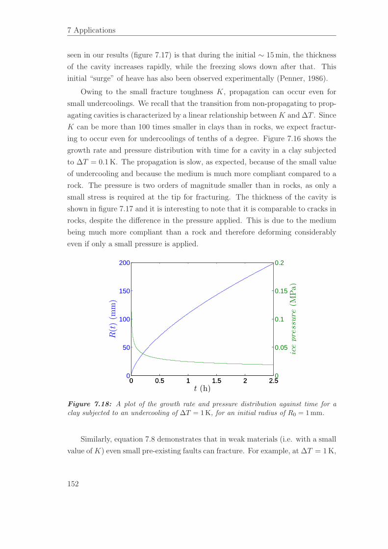
7 Applications
seen in our results (figure 7.17) is that during the initial ∼ 15 min, the thickness
of the cavity increases rapidly, while the freezing slows down after that. This
initial “surge” of heave has also been observed experimentally (Penner, 1986).
Owing to the small fracture toughness K, propagation can occur even for
small undercoolings. We recall that the transition from non-propagating to prop-
agating cavities is characterized by a linear relationship between K and ∆T . Since
K can be more than 100 times smaller in clays than in rocks, we expect fractur-
ing to occur even for undercoolings of tenths of a degree. Figure 7.16 shows the
growth rate and pressure distribution with time for a cavity in a clay subjected
to ∆T = 0.1 K. The propagation is slow, as expected, because of the small value
of undercooling and because the medium is much more compliant compared to a
rock. The pressure is two orders of magnitude smaller than in rocks, as only a
small stress is required at the tip for fracturing. The thickness of the cavity is
shown in figure 7.17 and it is interesting to note that it is comparable to cracks in
rocks, despite the difference in the pressure applied. This is due to the medium
being much more compliant than a rock and therefore deforming considerably
even if only a small pressure is applied.
0 0.5 1 1.5 2 2.50
50
100
150
200
t (h)
R(t
)(m
m)
0 0.5 1 1.5 2 2.50
0.05
0.1
0.15
0.2
ice
pre
ssure
(MPa)
Figure 7.18: A plot of the growth rate and pressure distribution against time for aclay subjected to an undercooling of ∆T = 1 K, for an initial radius of R0 = 1 mm.
Similarly, equation 7.8 demonstrates that in weak materials (i.e. with a small
value of K) even small pre-existing faults can fracture. For example, at ∆T = 1 K,
152
7.7 Fracturing of clays
an initial cavity of just R0 = 1 mm propagates rapidly as described in figure 7.18.
In this case, the pressures are still small compared to rocks but larger than in
figure 7.16. This is possible due to the higher value of undercooling and is nec-
essary for propagation because, although the fracture toughness is the same in
the two cases, the area over which the pressure is acting is much smaller in the
R0 = 1 mm case.
Watanabe (2002) performed experiments of freezing of a water-saturated pow-
der and found that the growth rate of ice lenses is proportional to the undercool-
ing, a relation that can also be seen in our figure 7.13 which, even though it uses
values representative of a rock, can be used to qualitatively describe soils too.
This indicates that, for the temperature range used in Watanabe’s experiments
(< 1◦ C), either no pore ice exists or its effect on the permeability was negligi-
ble. Indeed, Watanabe et al. (1997) observed the microstructure near the freezing
front of an ice lens in a soil and found no pore ice. The heaving rate in the silt, i.e.
the rate of the thickness increase of the ice lens, was found to be 1µm sec−1 ◦ C−1.
As we have found typical aspect ratios of ice lenses in soils to be about 10−3, we
deduce that this approximately corresponds to a fracturing rate of 0.1 mm min−1
◦ C−1, which is similar to what our theory predicts. As we mentioned earlier,
similar order of magnitude growth rates were observed by Style et al. (2011).
While there is some uncertainty over the exact values of initial cavity radius and
medium permeability used in the experiments, it is important to point out here
that these should not affect the agreement with the growth rates much. First of
all, we have seen that the growth rate of a crack is not very sensitive to the initial
radius (see section 6.6.3). Secondly, the value for the permeability used for the
examples shown in figures 7.16-7.18 is representative of a clay and close to the
critical value (Π ≈ 10−12 cm2) above which the effect of Π on the timescale of
the propagation becomes negligible (see also section 6.6.2). Clays are unlikely to
have permeabilities smaller than the ones used here, unless they are affected by
a large amount of pore ice, which wasn’t observed experimentally.
Some evidence also exists on the temperature required for the first ice lens
to grow. Watanabe (2002), during his experiments in a system of silica micro-
spheres, observed new ice lenses at an undercooling of just 0.02 K. Using a fracture
toughness of K = 102 Pa · m1/2 and an initial radius of R0 = 0.0011 cm (values
taken from Style et al., 2011), our theory predicts that the minimum temperature
153
7 Applications
for fracturing to occur is ∆T = 0.024 K. In experiments with kaolinite clay with
K = 1.5 MPa· m1/2 and R0 = 0.001 cm, Style et al. (2011) observed lenses forming
at temperatures of −0.3◦ C, where our theory predicts a minimum undercooling
of 0.37 K required for fracturing. The agreement with predictions from both ex-
periments is good. This reinforces the idea that ice lens formation in soils can be
described by ideas similar to fracturing in rocks, and our model seems to be in
good agreement with existing observations and experimental data in soils.
7.8 Conclusions
In this chapter, our aim has been to further explore the model developed and
solved in chapter 6 to understand some real-life situations of frost fracturing. We
have also discussed some existing models and determined ways in which our work
complements and extends past studies.
We have discussed the work of Walder & Hallet (1985) and compared our
predictions for the growth rate of a cavity to theirs. After incorporating some of
the features of their model in ours we have managed to achieve good agreement
and understand where the small differences in predictions come from. We have
also discussed some aspects of the work of Murton et al. (2006) and found that
our estimates for the minimum radii for propagation are in good agreement.
Extending the work done in chapter 6, we have studied the effect of several
parameters on the fracturing potential of an existing fault. This has led us to
some important conclusions about the properties required for a material to be
frost-proof. Interestingly, it is only the fracture toughness of the material and
the size of pre-existing faults that affect the potential for fracturing at a given
temperature, while all other material parameters can only affect the time scale of
the process once it occurs.
Following from the discussion of the existence of pore ice, motivated by the
work of Walder & Hallet (1985) and Murton et al. (2006), we have attempted
to incorporate a frozen fringe in our model. We suggested a rule to describe the
undercooling-dependent permeability and demonstrated the effect that a variable
154
7.8 Conclusions
permeability has on the propagation rate. The existence of pore ice is a non-
straightforward subject that requires a lot more theoretical work, coupled with
experimental evidence, which is beyond the scope of this thesis. We have shown
though that our model is flexible enough to include these ideas.
Finally, we have explained how our model can be used to describe fracturing in
clays, and analyzed the main features that differentiate this from rock fracturing.
With the studies of rock fracturing and frost heaving revealing many similarities
between the two processes, our work can serve as a theoretical model for the
analysis of a large variety of frost fracturing problems. Our model agrees with
experimental data of the prediction of the temperature needed for ice lenses to
grow, as well as evidence on ice lens growth rates. It also reproduces other features
that have been observed experimentally, such as the sudden surge of heave at the
initial stages of ice lens formation.
155

Chapter 8
Conclusions and future work
The aim of this thesis has been to study the phenomenon of frost fracturing
of rocks due to water freezing inside them at low temperatures, and develop a
theoretical model describing ice growth and crack propagation from fundamental
physical principles. We summarized past theoretical and experimental studies in
chapter 1, where we identified considerable progress in the theoretical modelling
of frost cracking. The important role played by unfrozen films of water between
ice and rock has been identified by several studies. The physics causing and
governing these films were presented in chapter 2. The balance of pressures across
these premelted films determines the fracturing of an ice-filled crack and forms
the basis of our theoretical model.
The first problem we discussed was that of ice growth inside a spherical cav-
ity in a porous, elastic medium. The aim of using this simple geometry was to
157
8 Conclusions and future work
compare the contributions of two different processes on the pressure acting on
the rock: the expansion of water during freezing, and the disjoining forces acting
across the thin premelted film in almost-filled cavities. The important conclu-
sion here was that the effect of expansion on the pressure applied to the rock is
negligible for media more permeable than about Π ≈ 10−15 cm2.
The ideas deduced from the spherical model allowed us to develop a theoretical
model for a more realistic geometry, concentrating on the important premelting
stage rather than the initial ice growth. The 3D penny-shaped crack problem,
first developed in chapter 4, was studied both in the framework of a similarity
solution for a warming environment, and as a time-dependent problem. Both
these approaches provided us with the opportunity to study the existence of
solutions for different values of the rock parameters, as well as the undercooling
of the environment. The different regimes were summarized in figure 5.7, and we
developed a criterion predicting whether a pre-existing fault will fracture. This
can be expressed in terms of the fracture toughness of the material, over the
undercooling of the environment
K
∆T<
2√π
R1/20
ρsLTm
. (8.1)
In the case where this condition is not met, ice can still grow inside the cavity
and deform it without fracturing it. The process continues with the thickness of
the cavity increasing until an equilibrium is reached where the disjoining pressure
between the ice and the rock is balanced by the elastic response of the medium.
We also established that for the permeability of the medium to affect the
fracturing potential of a fault, the undercooling of the environment needs to vary
with time. For example, in the case of a warming environment described in
chapter 5, the maximum value of K/∆T for which fracturing can occur behaves
as
β = max{K
H} ∼ Π1/4
(1 + Π)1/4. (8.2)
In cases with constant ∆T , the permeability of the medium only affects the
timescale of growth. In either situation, only permeabilities smaller than about
10−12 cm2 have an important effect on either the fracturing potential or the frac-
turing rate. A similar behaviour was found with the elastic modulus m, which
158
also affects only the timescale of the problem.
Another interesting result is associated with the initial size of a fault. As
expected, media with smaller faults are less prone to fracturing (see section 7.4.2)
as, due to their shorter length, larger pressure is required for the stress at the tip
to reach the critical value. We did see in section 6.6.3 though that the fracturing
rate of a crack is dependent only on its current size rather than its initial size,
which means that the growth curves of two cracks of different initial sizes will
coincide if all other parameters are the same.
General patterns of dependence of the growth curves of a cavity on different
parameters of the problem were established. The ratio of fracture toughness to
undercooling not only determines the susceptibility of a medium to fracturing,
but also strongly affects the propagation rate, with a larger K/∆T ratio resulting
in slower propagation. The growth rate is also proportional to the elastic modulus
of the medium, hence stiff rocks are expected to fracture quickly. The fast growth
rates ( mm/ sec) found for some rocks can be attributed to the fact that we have
considered the permeability of the medium to remain unchanged even for low
temperatures, but the concept of pore ice is easy to incorporate in our model.
We considered under which conditions a pore of a given size will become ice-
filled. This allowed us to construct an expression for the effective permeability
of a medium with pore ice as an attempt to quantify its effect on the water
flow through the medium. We found that, in the presence of pore ice, maximum
growth rates come from undercoolings of around 5 − 10◦ C. We believe that it
is important to establish a better understanding of the existence of pore ice in
frozen media, through either experimental or field observations.
An important point of the thesis is that the model developed here can also
be used to describe the growth of ice lenses in soils, as these have been observed
to have crack-like behaviour. Treating saturated soils as elastic media means
that ice lens growth is predicted without the need for a frozen fringe, which is in
agreement with observations. The results from our model agree with experimental
observations of the warmest temperature at which an ice lens can form. It is
also in good agreement with the order of magnitude of ice lens growth observed
in experiments. The surge in heave during early times, which has been seen
experimentally, is also present in our results.
159
8 Conclusions and future work
In conclusion, we have developed a theoretical model which we believe can
describe both fracturing in rocks as well as ice lens growth in cohesive soils. The
model is based on fundamental physical ideas, and explains the nature of the thin
films of water existing between ice and medium which are critical in the process
of fracturing. We have shown that different features can be incorporated into the
model, such as a variable permeability or temperature, to obtain results for specific
environmental conditions. Much experimental work done in previous decades
was focused around concepts such as the expansion of water upon freezing, which
resulted in the study of only specific parameters of the problem and environmental
conditions necessary for the expansion effect to be important. The existence of
a theoretical model and the analysis of the several parameters of the problem
that we have performed in this thesis can assist with steering future experimental
work in the right direction. In addition to this, if phenomena like pore ice or
freezing rates are found to be important, the model is capable of coupling a time-
dependent temperature with the resulting effective permeability to investigate
their effect on the growth rate of cracks.
While we believe that the penny-shaped geometry here is applicable to many
real-life situations, and we do not expect the results to be very sensitive to it,
the mathematical and physical ideas that we have developed can be modified
for different geometries too. For example, ice lenses in soils have been observed
to grow off vertical ice-filled cracks (Arenson et al., 2008; Style et al., 2011).
This indicates that a 2D wedge geometry could be applicable. Suitable solutions
for both the solid and liquid pressure fields can be found for a quarter plane
configuration, which could then be used to develop a similar model for the wedge
geometry.
160
Appendix A
Linear Elasticity
A.1 The biharmonic equation in cylindricals
In cylindricals, the equations relating the stress to the displacement can be written
in the form:
σrr = (λ + 2G)∂ur
∂r+ λ
ur
r+ λ
∂uz
∂z, (A.1)
σθθ = λ∂ur
∂r+ (λ + 2G)
ur
r+ λ
∂uz
∂z, (A.2)
σzz = λ∂ur
∂r+ λ
ur
r+ (λ + 2G)
∂uz
∂z, (A.3)
σrz = G
(∂ur
∂z+
∂uz
∂r
)
, (A.4)
161
A Linear Elasticity
where the subscripts represent components of the stress tensor σ and the displace-
ment vector u. Lame’s first parameter is represented by λ, while G is the shear
modulus. Now, if we let
ur =λ + G
GΦrz, (A.5)
uz =λ + 2G
G∇2Φ − λ + G
GΦzz, (A.6)
where the subscripts of the function Φ(r, z) describe partial differentiation. Then,
the expressions for the stress components become
σrr = λ∇2Φz − 2(λ + G)Φrrz, (A.7)
σzz = (3λ + 4G)∇2Φz − 2(λ + G)Φzzz, (A.8)
σθθ = ∇2Φz −2
r(λ + G)Φzr, (A.9)
σrz = (λ + 2G)∂
∂r∇2Φ − 2(λ + G)Φzzr, (A.10)
which, when substituted into the equilibrium equations, imply that Φ(r, z) must
satisfy the biharmonic equation:
∇4Φ = 0. (A.11)
A.2 Pressure and displacement fields in terms of Bessel
functions
We want to use the function Φ to find an expression relating the displacement and
press distribution fields. In cylindrical coordinates we note the following identity
∫∞
0
r∇2fJ0(ξr) dr =
(d2
dz2− ξ2
) ∫∞
0
rfJ0(ξr) dr. (A.12)
where J0 is the Bessel function of the first kind of order zero. If we use this with
f = ∇2Φ and then again with f = Φ we find
(d2
dz2− ξ2
)2
F (ξ, z) =
∫∞
0
r∇4ΦJ0(ξr) dr = 0, (A.13)
162
A.2 Pressure and displacement fields in terms of Bessel functions
where
F (ξ, z) =
∫∞
0
rΦJ0(ξr) dr. (A.14)
The solution to equation (A.13) is
F (ξ, z) = [A(ξ) + zB(ξ)] e−ξz, (A.15)
where we have assumed that Φ decays at infinity. Now, by multiplying equation
(A.5) by rJ1(ξr) and integrating from 0 to ∞ we find
∫∞
0
rurJ1(ξr) dr =λ + G
GξdF
dz. (A.16)
We use the following identity to invert the integral
∫∞
0
Jn(xu)(xu)1/2 du
∫∞
0
Jn(yu)(yu)1/2f(y) dy = f(x) for n ≥ −1
2(A.17)
and find an expression for ur:
ur =λ + G
G
∫∞
0
ξ2 dF
dzJ1(ξr) dξ. (A.18)
Similarly,
uz =
∫∞
0
ξ
(d2F
dz2− λ + 2G
Gξ2F
)
J0(ξr) dξ, (A.19)
σzz =
∫∞
0
ξ
[
(λ + 2G)d3F
dz3− (3λ + 4G)ξ2 dF
dz
]
J0(ξr) dξ, (A.20)
σrz =
∫∞
0
ξ2
[
λd2F
dz2+ (λ + 2G)ξ2F
]
J1(ξr) dξ (A.21)
,
σrr + σθθ = 2
∫∞
0
ξ
(
λd3F
dz3+ Gξ2 dF
dz
)
J0(ξr) dξ. (A.22)
We can use the equation of equilibrium
∂
∂r
(r2σrr
)= r(σrr + σθθ) − r2∂σrz
∂z. (A.23)
163
A Linear Elasticity
We substitute for the expressions for σrr + σθθ and σrz and integrate to find
σrr =
∫∞
0
ξ
[
λd3F
dz3+ (λ + 2G)ξ2 dF
dz
]
J0(ξr) dξ − 2(λ + G)
r
∫∞
0
ξ2 dF
dzJ1(ξr) dξ
(A.24)
and therefore
σθθ = λ
∫∞
0
ξ
(d3F
dz3− ξ2 dF
dz
)
J0(ξr) dξ +2(λ + G)
r
∫∞
0
ξ2 dF
dzJ1(ξr) dξ. (A.25)
164
Appendix B
Numerical method for time-dependent
penny-shaped problem
We use a mid-point rule to represent the cavity shape which means that inside
the nth interval
Bi =Bi
n + Bin+1
2(B.1)
at the i-th iteration in time. Then
∂Bi
∂η= N(Bi
n+1 − Bin) (B.2)
and∂Bi
n
∂t≈ Bi − Bi−1
∆t=
Bin + Bi
n+1 − Bi−1n − Bi−1
n+1
2∆t(B.3)
We will treat the interval which includes the tip of the ice a bit more care-
fully. We define Λ = ⌈λN⌉, so that the ice tip is in the Λth interval. Then, we
165
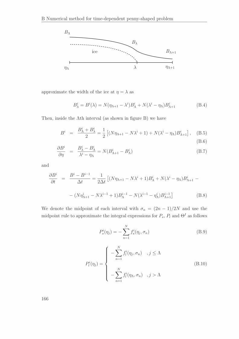
B Numerical method for time-dependent penny-shaped problem
ηΛ λ ηΛ+1
BΛ
Bλ
BΛ+1ice
approximate the width of the ice at η = λ as
Biλ = Bi(λ) = N(ηΛ+1 − λi)Bi
Λ + N(λi − ηΛ)BiΛ+1 (B.4)
Then, inside the Λth interval (as shown in figure B) we have
Bi =Bi
Λ + Biλ
2=
1
2
[(NηΛ+1 − Nλi + 1) + N(λi − ηΛ)Bi
Λ+1
], (B.5)
(B.6)
∂Bi
∂η=
Biλ − Bi
Λ
λi − ηΛ
= N(BiΛ+1 − Bi
Λ) (B.7)
and
∂Bi
∂t=
Bi − Bi−1
∆t=
1
2∆t
[(NηΛ+1 − Nλi + 1)Bi
Λ + N(λi − ηΛ)BiΛ+1 −
− (NηiΛ+1 − Nλi−1 + 1)Bi−1
Λ − N(λi−1 − ηiΛ)Bi−1
Λ+1
](B.8)
We denote the midpoint of each interval with σn = (2n − 1)/2N and use the
midpoint rule to approximate the integral expressions for Ps, Pl and ΘI as follows
P is(ηj) = −
N∑
n=1
f is(ηj, σn) (B.9)
P il (ηj) =
−N∑
n=1
f il (ηj, σn) , j ≤ Λ
−N∑
n=1
f il (ηΛ, σn) , j > Λ
(B.10)
166

ΘI i(ηj) =
Λi−1∑
n=1
f il (ηj, σn) + f i
l (ηj, σiλ) (B.11)
where σiλ = (ηΛi + λi)/2. The new functions f i
s and f il that we have introduced
are given by
f is(ηj, σn) =
1
σn
M∗
(ηj
σn
)
(Bin+1 − Bi
n) (B.12)
f il (ηj, σn) = αjnR
i{[
(2n + 1)Ri − 2nRi−1]Bi
n − RiBi−1n +
+[(3 − 2n)Ri + (2n − 2)Ri−1
]Bi
n+1 − RiBi−1n+1
}(B.13)
(B.14)
and
f il (ηj, σ
iλ) = αjλR
i{[
(3NηΛ − Nλi + 4)Ri + 2(NηΛ + 1)Ri−1]Bi
Λ
+ −(NηΛ − Nλi + 2)RiBi−1Λ +
[N(λi − 3ηΛ)Ri + 2NηΛRi−1
]Bi
Λ+1 −+ −N(λi − ηΛ)RiBi−1
Λ+1
}(B.15)
(B.16)
We now have
P is(ηj) =
N∑
n=1
(µjn − µj(n−1))Bin where µjn =
1
σn
M∗
(ηj
σn
)
(B.17)
P il (ηj) =
−N∑
n=1
(αjnβin + αj(n−1)γ
in)Bi
n +N∑
n=1
(αjn + αj(n−1))Ri2Bi−1
n , j ≤ Λ
−N∑
n=1
(αΛnβin + αΛ(n−1)γ
in)Bi
n +N∑
n=1
(αΛn + αΛ(n−1))Ri2Bi−1
n , j > Λ
(B.18)
with
αjn =1
2N∆t
σn
ηj + σn
K
(2√
ηjσn
ηj + σn
)
andβi
n = (2n + 1)Ri2 − 2nRiRi−1
γin = (5 − 2n)Ri2 − (2n − 4)RiRi−1
(B.19)
167
B Numerical method for time-dependent penny-shaped problem
ΘI i(ηj) =
Λ−1∑
n=1
(αjnβin + αj(n−1)γ
in)Bi
n + (αj(Λ−1)γiΛ + αi
jλβiλ)B
iΛ + αi
jλγiλB
iΛ+1 −
−Λ−1∑
n=1
(αjn + αj(n−1))Ri2Bi−1
n − (αj(Λ−1)Ri2 + αi
jλδiλ)B
i−1Λ − αi
jλǫiλB
i−1Λ+1
(B.20)
where
αijλ =
λi − ηΛ
2∆t
σλ
ηj + σλ
K
(2√
ηjσλ
ηj + σλ
)
(B.21)
βiλ = (3NηΛ − Nλi + 4)Ri2 − 2(NηΛ + 1)RiRi−1 (B.22)
γiλ = N(λi − 3ηΛ)Ri2 + 2NηΛRiRi−1 (B.23)
δiλ = (NηΛ − Nλi + 2)Ri2 (B.24)
ǫiλ = N(λi − ηΛ)Ri2 (B.25)
(B.26)
Pressure balance:
P is(ηj) − P i
l (ηj) =
= HK−1 − ΠΘI i(ηj) if j < Λ
= N(λi − ηΛ)(
HK−1 − ΠΘI i(ηj)
)
if j = Λ
= 0 if j > Λ
(B.27)
168
Appendix C
Method for estimating integrals over
intervals with pole singularities
In general, we integrate numerically by using a gaussian quadrature, which can
deal with weak singularities at an endpoints c like log(x−c) and 1/√
x − c. Some
intervals though require special treatment because they have stronger singulari-
ties. The kernel M(η/σ) has a pole singularity at σ = η. The elliptic integrals
K(z) and E(z) have the following expansions around z = 1:
K(z) ≈ −1
2log (1 − z) (1 + O(z − 1)) + log 4 + O(z − 1) (C.1)
and
E(z) ≈ 1 + log (1 − z)O(z − 1) + O(z − 1), (C.2)
hence the singularities are at most logarithmic. For Snn and Tnn (i.e. the intervals
that include the pole singularity) we use the following method. Suppose we want
169
C Method for estimating integrals over intervals with pole singularities
to integrate
I = −∫ ηn
ηn−1
f(σ, η) dσ
(σ − η)√
1 − σ2= I− + I+ = (C.3)
= limǫ→0+
[∫ η−ǫ
ηn−1
f1(σ, η) dσ
(σ − η)√
1 − σ2+
∫ ηn
η+ǫ
f2(σ, η) dσ
(σ − η)√
1 − σ2
]
.(C.4)
We want to subtract the singularity in order to be left with some integral that
can be integrated numerically using a gaussian quadrature. To do so, we subtract
the residue in the following way:
I− =
∫ η−ǫ
ηn−1
f1(σ, η) − f1(η, η)
(σ − η)√
1 − σ2dσ + f1(η, η)
∫ η−ǫ
ηn−1
dσ
(σ − η)√
1 − σ2=
≈∫ η−ǫ
ηn−1
f1′(σ, η)√1 − σ2
dσ + f1(η, η)
∫ η−ǫ
ηn−1
dσ
(σ − η)√
1 − σ2, (C.5)
which then gives for the whole integral
I =
∫ η
ηn−1
f1′(σ, η)√1 − σ2
dσ +
∫ ηn
η
f2′(σ, η)√1 − σ2
dσ + f(η, η)−∫ ηn
ηn−1
dσ
(σ − η)√
1 − σ2, (C.6)
where f(η, η) = f1(η, η) = f2(η, η) since f(σ, η) is continuous at σ = η. The last
integral is a Cauchy principal value integral and when evaluated gives
−∫ ηn
ηn−1
dσ
(σ − η)√
1 − σ2=
1√
1 − η2log
(
1 +√
1 − η2√
1 − η2n−1 − ηηn−1
1 +√
1 − η2√
1 − η2n − ηηn
)
.
(C.7)
The remaining integrals are approximated numerically using a Gaussian quadra-
ture since their singularities are weak enough. This analysis can be applied for
both Snn and Tnn.
170
Appendix D
Assumption of uniform pressure in the
tip of the crack
In chapter 5, we used the thin film approximation inside all of the cavity in
order to describe the flow of water. This assumed that both the premelted film
occupying r < λR as well as the cavity at r > λR are thin enough for the flow
along them to be negligible. If this is not true for the r > λR region, we can
instead use the uniform pressure assumption, which implies that the flow along
the cavity dominates the flow from the porous medium into the cavity, so that any
pressure variations are evened out quickly. These two ideas represent the opposite
ends of the spectrum but we will see that they make only a small difference to
the overall characteristics of the problem.
The liquid pressure in the porous medium is given as an integral of the flux
171
D Assumption of uniform pressure in the tip of the crack
into the cavity q(r, t)
pl(r, t) =1
π
µ
Π
∫ R(t)
0
K
(2√
rs
r + s
)
q(s, t)s ds
s + r, (D.1)
The flux is related to the derivative of the liquid pressure through
q(r, t) = −2Π
µlimz→0
∂p
∂z(D.2)
and for the ice-occupied region, lubrication theory gives
q(r, t) = −2Π
µlimz→0
∂p
∂z= −2
∂b
∂t. (D.3)
The liquid pressure now becomes
pl(r, t) = − 2
π
µ
Π
∫ λR(t)
0
K
(2√
rs
r + s
)∂b
∂t
s ds
s + r−
− 2
π
µ
Π
∫ R(t)
λR(t)
K
(2√
rs
r + s
)∂pl
∂z
∣∣∣∣z=0
s ds
s + r, (D.4)
with the condition of uniform pressure in the water-filled tip of the crack
pl(r, t) = pl(λR, t) for r > λR. (D.5)
Following the same process as in chapter 5, we can write down the equations
describing the similarity solution for ∆T = Ht−1/4. The dimensionless liquid
pressure is given by
Pl(η) = −k2
∫ λ
0
K
(2√
ησ
η + σ
) [1
4B(σ) − 1
2σB′(σ)
]σdσ
η + σ−
−2k
π
∫ 1
λ
K
(2√
ησ
η + σ
)
P zl (σ)
σdσ
η + σ, (D.6)
where we denote P zl (σ) =
∂Pl(σ, z)
∂z
∣∣∣∣z=0
. The temperature is given by equa-
172
tion (5.23) as in chapter 5, hence the liquid pressure can be written as
Pl(η) = −ΘI(η) − 2k
π
∫ 1
λ
K
(2√
ησ
η + σ
)
P zl (σ)
σdσ
η + σ≡ −ΘI(η) − Φ(η). (D.7)
The pressure balance can then be re-written as
Ps(η) = (Π + 1)Pl(η) + ΠΦ(η) + ΠC for η < λ.
= Pl(η) for η > λ. (D.8)
We use the same discretization method as in section 5.2.1. The difference
here is that since the terms P zl cannot be written in terms of the cavity thickness
B, they have to be determined from the matrix problem. The simplest way
to write it is to assume 2N unknowns, [B1, ...BN ] and [Pl1 , ...PlΛ , P zlΛ+1
, ...P zlN
],
where Pln = Pl(ηn). We have N conditions from the expression for the liquid
pressure (D.7)
δjnPln +8k
π
N∑
n=Λ+1
(λjn + νjn)P zln + k2
Λ−1∑
n=1
(λjn + νj(n−1))Bn +
+k2(νj(n−1) + Iλj )BΛ + k2Jλ
j BΛ+1 = 0, (D.9)
which is valid for j ≤ Λ, while for j > Λ the first term is replaced by PlΛ to
account for the uniform pressure condition in the water-filled tip. The pressure
balance in the ice-filled region provides us with a further Λ conditions for j ≤ Λ
(Π + 1)δjnPln +8k
πΠ
N∑
n=Λ+1
(λjn + νjn)P zln −
−∑
n=1
(µjn − µj(n−1))Bn = −ΠC, (D.10)
while for j > Λ we have the following N − Λ conditions
PlΛ −∑
n=1
(µjn − µj(n−1))Bn = 0. (D.11)
The 2N linear relations described by equations (D.9)-(D.11) replace the matrix
equation of section 5.2.1.
173
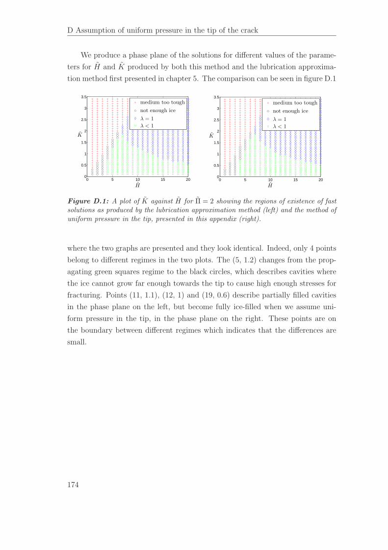
D Assumption of uniform pressure in the tip of the crack
We produce a phase plane of the solutions for different values of the parame-
ters for H and K produced by both this method and the lubrication approxima-
tion method first presented in chapter 5. The comparison can be seen in figure D.1
0 5 10 15 200
0.5
1
1.5
2
2.5
3
3.5
H
K
medium too tough
not enough ice
λ = 1
λ < 1
0 5 10 15 200
0.5
1
1.5
2
2.5
3
3.5
H
K
medium too tough
not enough ice
λ = 1
λ < 1
Figure D.1: A plot of K against H for Π = 2 showing the regions of existence of fastsolutions as produced by the lubrication approximation method (left) and the method ofuniform pressure in the tip, presented in this appendix (right).
where the two graphs are presented and they look identical. Indeed, only 4 points
belong to different regimes in the two plots. The (5, 1.2) changes from the prop-
agating green squares regime to the black circles, which describes cavities where
the ice cannot grow far enough towards the tip to cause high enough stresses for
fracturing. Points (11, 1.1), (12, 1) and (19, 0.6) describe partially filled cavities
in the phase plane on the left, but become fully ice-filled when we assume uni-
form pressure in the tip, in the phase plane on the right. These points are on
the boundary between different regimes which indicates that the differences are
small.
174
Appendix E
Freezing temperature depression of a
spherical nucleus in a spherical pore
Consider a spherical pore of radius R with ice growing inside it. Two effects
contribute to the depression of the freezing temperature: the curvature of the
spherical ice nucleus, and the disjoining forces which become important when the
pore is almost filled with ice. This is shown by the following relation
ρsLTm − T
Tm
= pT + κγ =A
6π(R − a)3+
2γ
a, (E.1)
where we have assumed that the ice is also spherical, with radius a. The depression
of T due to curvature melting decreases as the ice grows, whereas the disjoining
pressure pT becomes larger the closer the ice is to the rock. Since these two
effects act in opposing ways, there is a radius of ice for which the depression of
175
E Freezing temperature depression of a spherical nucleus in a spherical pore
the freezing temperature is minimised. This is of interest when considering the
existence of pore ice in a porous medium. If the minimum Tm − T occurs for
an almost ice-filled cavity, we can assume that at a given undercooling all pores
larger than a given size are completely ice-filled, while the smaller ones are devoid
of ice. It is also useful to determine which term dominates the depression of the
temperature at that stage. Minimising the right-hand-side of equation (E.1) with
respect to a, we find
(R − a)4 − A4πγ
a2 = 0. (E.2)
Defining c = A/(4πγ), we find
R = a ± c1/4a1/2. (E.3)
Setting x = a1/2 we have two quadratic equations for x
x2 ± c1/4x − R = 0 (E.4)
with four solutions
x =∓c1/4 ±
√c1/2 + 4R
2. (E.5)
Of these solutions, only one satisfies 0 < a < R (the first minus and the second
plus) and gives
amin = R +1
2c1/4
(
c1/4 −√
c1/2 + 4R)
. (E.6)
For typical values of the parameters, R is about 7 orders of magnitude larger than
c1/2 which means that we can expand the square root to find
amin = R − c1/4R1/2 +1
2c1/2 + c1/4O(ǫ2), (E.7)
where ǫ2 = c1/2/R = O(10−7) and the terms on the right-hand-side are ordered
in decreasing size. This shows that the first and second order terms are R(1− ǫ),
where ǫ = O(10−3) − O(10−4). Substituting into equation (E.1) we find the
176
minimum undercooling
minρsL∆T
2γTm
=1
3c(R − amin)
−3 + a−1min
=1
3c(c1/4R1/2 − 1
2c1/2)−3 + (R − c1/4R1/2 +
1
2c1/2)−1
=1
3c1/4R−3/2(1 − O(ǫ))−3 + R−1(1 − O(ǫ))−1
= R−1O(ǫ)(1 − O(ǫ)) + R−1(1 + O(ǫ))
= R−1(1 + O(ǫ)), (E.8)
which shows that the largest contribution comes from the curvature melting term,
and it is 3–4 orders of magnitude larger than the disjoining forces effect. In
conclusion, the above analysis shows that the minimum temperature depression
is found for ice which is as large as possible (to minimize curvature melting effect)
but not close enough to the rock to cause the disjoining pressure effect to become
large. This occurs for ice which is 10−3R − 10−4R away from the pore boundary,
hence the pore can be considered ice-filled when we discuss the effect of pore ice
on the permeability of the medium.
177

Bibliography
Akagawa, S., Satoh, M., Kanie, S. & Mikami, T. 2006 Effect of tensile
strength on ice lens initiation temperature. ASCE.
Al-Shayea, N.A. 2004 Effects of testing methods and conditions on the elastic
properties of limestone rock. Engineering geology 74 (1-2), 139–156.
Arenson, L.U., Azmatch, T.F., Sego, D.C. & Biggar, KW 2008 A new
hypothesis on ice lens formation in frost-susceptible soils. In Proceedings of the
Ninth International Conference on Permafrost, Fairbanks, Alaska, June 29–
July 3, 2008 .
Atkinson, B.K. 1984 Subcritical crack growth in geological materials. Journal
of Geophysical Research 89 (B6), 4077–4114.
Atkinson, BK & Rawlings, RD 1981 Acoustic emission during stress corro-
sion cracking in rocks. Richards, PG (Ed.), Earthquake prediction pp. 605–616.
179
Bibliography
Battle, WRB 1960 Temperature observations in bergschrunds and their rela-
tionship to frost shattering. Norwegian cirque glaciers 4, 83–95.
Bear, J. 1988 Dynamics of fluids in porous media. Dover publications.
Center, Hilton Pond 2000 Frost heave.
Charles, RJ 1958 Static fatigue of glass. i. Journal of Applied Physics 29 (11),
1549–1553.
Davis, S.H. 2001 Theory of solidification. Cambridge Univ Pr.
Embleton, C. & King, C.A. 1975 SERIES TITLE: YEAR: 1975 .
Everett, D.H. 1961 The thermodynamics of frost damage to porous solids.
Transactions of the Faraday Society 57, 1541–1551.
Faraday, M. 1859 Note on regelation. Proceedings of the Royal Society of London
10, 440–450.
Fowler, AC 1989 Secondary frost heave in freezing soils. SIAM Journal on
Applied Mathematics pp. 991–1008.
Fowler, A.C. & Krantz, W.B. 1994 A generalized secondary frost heave
model. Siam Journal on Applied Mathematics pp. 1650–1675.
Freiman, SW 1984 Effects of chemical environments on slow crack growth in
glasses and ceramics. Journal of Geophysical Research 89 (B6), 4072–4076.
Fukuda, M. 1983 The pore water pressure profile in porous rocks during freez-
ing. In Proceedings. Fourth International Conference on Permafrost. National
Academy Press, Washington, DC , , vol. 322, p. 327.
de Gennes, P.G. 1985 Wetting: statics and dynamics. Reviews of Modern
Physics 57 (3), 827.
Gilpin, R.R. 1979 A model of the “liquid-like”layer between ice and a substrate
with applications to wire regelation and particle migration. J. Colloid Interface
Sci 68, 235–251.
180
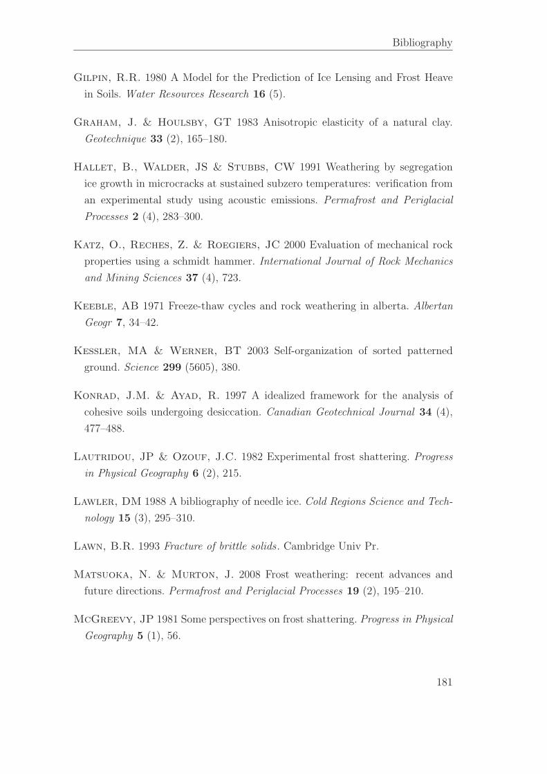
Bibliography
Gilpin, R.R. 1980 A Model for the Prediction of Ice Lensing and Frost Heave
in Soils. Water Resources Research 16 (5).
Graham, J. & Houlsby, GT 1983 Anisotropic elasticity of a natural clay.
Geotechnique 33 (2), 165–180.
Hallet, B., Walder, JS & Stubbs, CW 1991 Weathering by segregation
ice growth in microcracks at sustained subzero temperatures: verification from
an experimental study using acoustic emissions. Permafrost and Periglacial
Processes 2 (4), 283–300.
Katz, O., Reches, Z. & Roegiers, JC 2000 Evaluation of mechanical rock
properties using a schmidt hammer. International Journal of Rock Mechanics
and Mining Sciences 37 (4), 723.
Keeble, AB 1971 Freeze-thaw cycles and rock weathering in alberta. Albertan
Geogr 7, 34–42.
Kessler, MA & Werner, BT 2003 Self-organization of sorted patterned
ground. Science 299 (5605), 380.
Konrad, J.M. & Ayad, R. 1997 A idealized framework for the analysis of
cohesive soils undergoing desiccation. Canadian Geotechnical Journal 34 (4),
477–488.
Lautridou, JP & Ozouf, J.C. 1982 Experimental frost shattering. Progress
in Physical Geography 6 (2), 215.
Lawler, DM 1988 A bibliography of needle ice. Cold Regions Science and Tech-
nology 15 (3), 295–310.
Lawn, B.R. 1993 Fracture of brittle solids. Cambridge Univ Pr.
Matsuoka, N. & Murton, J. 2008 Frost weathering: recent advances and
future directions. Permafrost and Periglacial Processes 19 (2), 195–210.
McGreevy, JP 1981 Some perspectives on frost shattering. Progress in Physical
Geography 5 (1), 56.
181
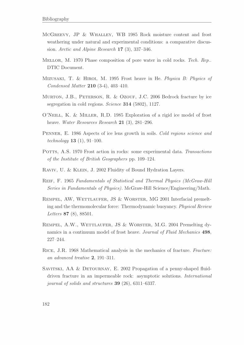
Bibliography
McGreevy, JP & Whalley, WB 1985 Rock moisture content and frost
weathering under natural and experimental conditions: a comparative discus-
sion. Arctic and Alpine Research 17 (3), 337–346.
Mellor, M. 1970 Phase composition of pore water in cold rocks. Tech. Rep..
DTIC Document.
Mizusaki, T. & Hiroi, M. 1995 Frost heave in He. Physica B: Physics of
Condensed Matter 210 (3-4), 403–410.
Murton, J.B., Peterson, R. & Ozouf, J.C. 2006 Bedrock fracture by ice
segregation in cold regions. Science 314 (5802), 1127.
O’Neill, K. & Miller, R.D. 1985 Exploration of a rigid ice model of frost
heave. Water Resources Research 21 (3), 281–296.
Penner, E. 1986 Aspects of ice lens growth in soils. Cold regions science and
technology 13 (1), 91–100.
Potts, A.S. 1970 Frost action in rocks: some experimental data. Transactions
of the Institute of British Geographers pp. 109–124.
Raviv, U. & Klein, J. 2002 Fluidity of Bound Hydration Layers.
Reif, F. 1965 Fundamentals of Statistical and Thermal Physics (McGraw-Hill
Series in Fundamentals of Physics). McGraw-Hill Science/Engineering/Math.
Rempel, AW, Wettlaufer, JS & Worster, MG 2001 Interfacial premelt-
ing and the thermomolecular force: Thermodynamic buoyancy. Physical Review
Letters 87 (8), 88501.
Rempel, A.W., Wettlaufer, JS & Worster, M.G. 2004 Premelting dy-
namics in a continuum model of frost heave. Journal of Fluid Mechanics 498,
227–244.
Rice, J.R. 1968 Mathematical analysis in the mechanics of fracture. Fracture:
an advanced treatise 2, 191–311.
Savitski, AA & Detournay, E. 2002 Propagation of a penny-shaped fluid-
driven fracture in an impermeable rock: asymptotic solutions. International
journal of solids and structures 39 (26), 6311–6337.
182
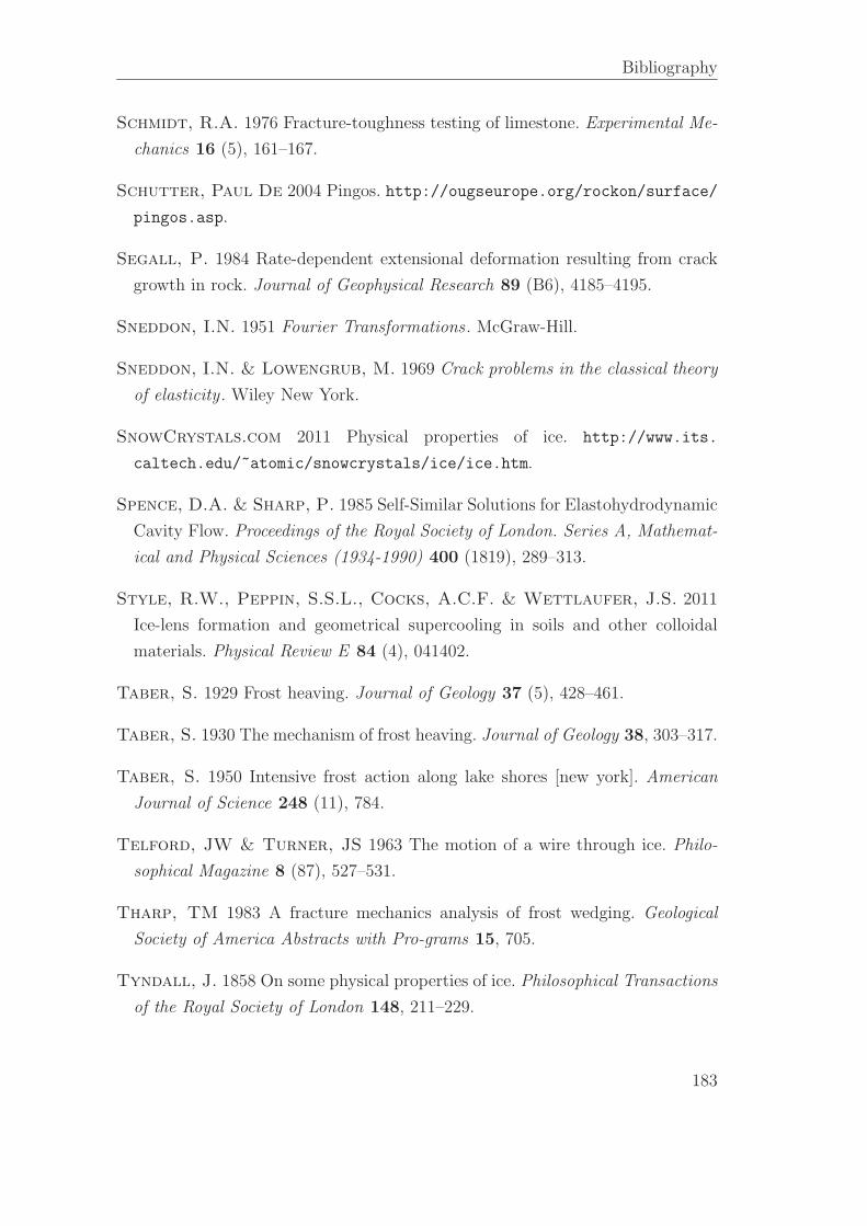
Bibliography
Schmidt, R.A. 1976 Fracture-toughness testing of limestone. Experimental Me-
chanics 16 (5), 161–167.
Schutter, Paul De 2004 Pingos. http://ougseurope.org/rockon/surface/
pingos.asp.
Segall, P. 1984 Rate-dependent extensional deformation resulting from crack
growth in rock. Journal of Geophysical Research 89 (B6), 4185–4195.
Sneddon, I.N. 1951 Fourier Transformations. McGraw-Hill.
Sneddon, I.N. & Lowengrub, M. 1969 Crack problems in the classical theory
of elasticity . Wiley New York.
SnowCrystals.com 2011 Physical properties of ice. http://www.its.
caltech.edu/~atomic/snowcrystals/ice/ice.htm.
Spence, D.A. & Sharp, P. 1985 Self-Similar Solutions for Elastohydrodynamic
Cavity Flow. Proceedings of the Royal Society of London. Series A, Mathemat-
ical and Physical Sciences (1934-1990) 400 (1819), 289–313.
Style, R.W., Peppin, S.S.L., Cocks, A.C.F. & Wettlaufer, J.S. 2011
Ice-lens formation and geometrical supercooling in soils and other colloidal
materials. Physical Review E 84 (4), 041402.
Taber, S. 1929 Frost heaving. Journal of Geology 37 (5), 428–461.
Taber, S. 1930 The mechanism of frost heaving. Journal of Geology 38, 303–317.
Taber, S. 1950 Intensive frost action along lake shores [new york]. American
Journal of Science 248 (11), 784.
Telford, JW & Turner, JS 1963 The motion of a wire through ice. Philo-
sophical Magazine 8 (87), 527–531.
Tharp, TM 1983 A fracture mechanics analysis of frost wedging. Geological
Society of America Abstracts with Pro-grams 15, 705.
Tyndall, J. 1858 On some physical properties of ice. Philosophical Transactions
of the Royal Society of London 148, 211–229.
183
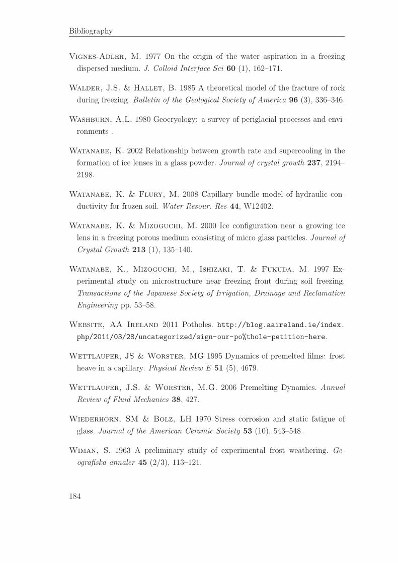
Bibliography
Vignes-Adler, M. 1977 On the origin of the water aspiration in a freezing
dispersed medium. J. Colloid Interface Sci 60 (1), 162–171.
Walder, J.S. & Hallet, B. 1985 A theoretical model of the fracture of rock
during freezing. Bulletin of the Geological Society of America 96 (3), 336–346.
Washburn, A.L. 1980 Geocryology: a survey of periglacial processes and envi-
ronments .
Watanabe, K. 2002 Relationship between growth rate and supercooling in the
formation of ice lenses in a glass powder. Journal of crystal growth 237, 2194–
2198.
Watanabe, K. & Flury, M. 2008 Capillary bundle model of hydraulic con-
ductivity for frozen soil. Water Resour. Res 44, W12402.
Watanabe, K. & Mizoguchi, M. 2000 Ice configuration near a growing ice
lens in a freezing porous medium consisting of micro glass particles. Journal of
Crystal Growth 213 (1), 135–140.
Watanabe, K., Mizoguchi, M., Ishizaki, T. & Fukuda, M. 1997 Ex-
perimental study on microstructure near freezing front during soil freezing.
Transactions of the Japanese Society of Irrigation, Drainage and Reclamation
Engineering pp. 53–58.
Website, AA Ireland 2011 Potholes. http://blog.aaireland.ie/index.
php/2011/03/28/uncategorized/sign-our-po%thole-petition-here.
Wettlaufer, JS & Worster, MG 1995 Dynamics of premelted films: frost
heave in a capillary. Physical Review E 51 (5), 4679.
Wettlaufer, J.S. & Worster, M.G. 2006 Premelting Dynamics. Annual
Review of Fluid Mechanics 38, 427.
Wiederhorn, SM & Bolz, LH 1970 Stress corrosion and static fatigue of
glass. Journal of the American Ceramic Society 53 (10), 543–548.
Wiman, S. 1963 A preliminary study of experimental frost weathering. Ge-
ografiska annaler 45 (2/3), 113–121.
184
Bibliography
Worster, MG 2000 Perspectives in Fluid Dynamics – a Collective Introduction
to Current Research, chap. Solidification of Fluids, pp. 393–446. CUP.
Zhu, D.M., Vilches, O.E., Dash, J.G., Sing, B. & Wettlaufer, J.S.
2000 Frost Heave in Argon. Physical Review Letters 85 (23), 4908–4911.
185


