WP/03/229

Free Trade Areas and Rules of Origin: Economics and Politics

Rupa Duttagupta and Arvind Panagariya

© 2003 International Monetary Fund WP/03/229

IMF Working Paper

Research Department

Free Trade Areas and Rules of Origin: Economics and Politics

Prepared by Rupa Duttagupta and Arvind Panagariya1

Authorized for distribution by Peter Clark

November 2003

Abstract

The views expressed in this Working Paper are those of the author(s) and do not necessarily represent those of the IMF or IMF policy. Working Papers describe research in progress by the author(s) and are published to elicit comments and to further debate.

Incorporating intermediate inputs into a small-union general-equilibrium model, this paper first develops the welfare economics of preferential trading under the rules of origin (ROO) and then demonstrates that the ROO could improve the political viability of Free Trade Agreements (FTAs). Two interesting outcomes are derived. First, a welfare reducing FTA that was rejected in the absence of the ROO becomes feasible in the presence of these rules. Second, a welfare improving FTA that was rejected in the absence of the ROO is endorsed in their presence, but upon endorsement it becomes welfare inferior relative to the status quo. JEL Classification Numbers: F10 Keywords: Rules of Origin, FTA, Welfare, Political economy Authors’ E-Mail Address: rduttagupta@imf.org, apanagari@econ.umd.edu

1 The authors are at the International Monetary Fund (rduttagupta@imf.org) and Department of Economics, University of Maryland at College Park (panagari@econ.umd.edu), respectively. They would like to thank Rachel Kranton, Jose Pineda, Francisco Rodriguez and Robert Schwab and the seminar participants at the World Bank Research Department, Columbia University and Michigan State University for many useful suggestions.

- 2 -

Contents Page

I. Introduction ................................................................................................................................. 3 II. The Model .................................................................................................................................. 5

The Pattern of Trade under MFN Tariffs ................................................................................. 7

III. The Economics and Politics of FTAs in the Absence of ROOs ............................................. 10 IV. The Economic Effects of the Rules of Origin ........................................................................ 13

A. Effects of the ROO: Positive Analysis ................................................................................. 14

B. Effects of the ROO: Welfare................................................................................................. 17

V. Political Viability of FTA with ROO....................................................................................... 18 A. ROOs, FTA Viability and Welfare....................................................................................... 19

B. ROO, FTA Viability and Welfare: Numerical Examples..................................................... 20

C. Extensions............................................................................................................................. 23

Extension 1. Both HC and FC Import Good 2 ....................................................................... 24

Extension 2. Endogenous determination of external tariffs in the post FTA equilibrium ..... 24

Extension 3. Exogenously given positive tariffs on final good and intermediate input......... 25

VI. Conclusion .............................................................................................................................. 25 References..................................................................................................................................... 27

- 3 -

I. INTRODUCTION

The rules of origin (ROOs) are an integral part of Free Trade Areas (FTAs): union members confer duty-free status on a product only if a pre-specified proportion of its value added originates within the union. Though it is generally recognized that ROOs make FTAs politically more acceptable, there is practically no formal analysis supporting this proposition.2 Since intermediate inputs are rarely incorporated into the formal models of FTAs, the recent political-economy-theoretic literature, including the pioneering contribution by Grossman and Helpman (1995) and the important paper by Krishna (1998), leaves the role of ROOs entirely out of consideration.3, 4 This paper accomplishes two broad objectives. First, incorporating intermediate inputs into the analysis, it derives the welfare implications of FTAs in the presence of the ROO. Second and more importantly, the impact of the ROO on the political feasibility of FTAs is then analyzed, and it is shown that the ROO could make FTAs more feasible. The analysis is conducted within a conventional general-equilibrium model that has three final goods and an intermediate input used in the production of one of the final goods. One partner country is assumed to import the input and export the final good using the input. The other partner country exports the input and imports the final good, thereby opening the way for the exchange of a tariff preference in the final good for a ROO. It is important to clarify that the exchange of a tariff preference for the ROO in the above model is only a part of the overall story of the politics of FTAs. The latter is inevitably multifaceted, aspects of which were analyzed by Helpman and Grossman (1995), Krishna (1998) and others.

2 The nascent literature on ROOs includes Krishna and Krueger (1995), Ju and Krishna (1998) and Falvey and Reed (1997, 1998). In addition, Panagariya and Krishna (forthcoming), who generalize the Kemp-Vanek-Ohyama-Wan proposition on necessarily welfare-enhancing customs unions to FTAs, discuss the rules of origin necessary to support welfare-enhancing FTAs.

3 Two recent surveys of the traditional and modern theoretical literature on preferential trade areas (PTAs) are Bhagwati and Panagariya (1996) and Panagariya (2000). Among the recent contributions to the literature, mention may be made of Baldwin (1995), Bhagwati (1993), Bond and Syropoulos (1996), Cadot, de Melo and Olarreaga (1999), Ethier (1998), Krugman (1991), Levy (1997), Panagariya and Findlay (1998), and Yi (1996).

4 Grossman and Helpman (1994) discuss the politics of tariff protection in the presence of intermediate inputs, but do not analyze FTAs in the context of input based ROO. Grossman and Helpman (1995) allow for ROOs that prevent transshipment of goods imported by a lower tariff member to the higher tariff member. In contrast, this paper focuses on ROOs based on input usage. Cadot, demelo and Olarreaga (2000) analyze the political economy of protection on intermediate inputs, in the presence of duty-drawback systems.

- 4 -

As such, this paper should be viewed as contributing to the understanding of one aspect of the overall story, although an important one. The setting captures a particularly relevant aspect of the recent wave of FTAs between developed and developing countries such as the North American Free Trade Agreement (NAFTA) in which the developing country member typically exports final goods that use inputs exported by the developed country member.5 Policy papers, particularly writings by Anne Krueger, have strongly emphasized the role played by the ROO in these FTAs. A key welfare result is that in general a ROO has an ambiguous effect on the welfare of union members individually as well as jointly. First consider the case in which the preference in the final good results in trade diversion. In the input market, the ROO diverts trade by substituting within-union supply for outside-union supply. But in the final-good market, it reverses trade diversion by making the within-union production of the good more costly relative to when the ROO were absent. Thus, the net effect is ambiguous.6 If the ROO is weakly binding on the price of the input, a tightening of it improves joint welfare because the loss from the price distortion in the intermediate input market is second-order small whereas the benefit from reversing trade diversion in the final good is finite. However, as the ROO is tightened further, the loss from the input price distortion is larger and may eventually offset the benefit in the final good market. However, if the tariff preference in the final good is purely trade creating such that the post-FTA price is at its free trade level, a binding ROO turns out to be unambiguously harmful. In this case, there is no trade diversion in the final good to be reversed whereas the ROO does lead to trade diversion in the input market. The political-economy analysis of FTAs is developed in three steps. First, using the original Grossman-Helpman (1994) model, the structure of tariffs in the initial equilibrium is determined. The key result here is that the tariff on the input is zero in both partners.7 Second, the viability of an FTA is studied, in the absence of the ROOs. Third, it is analyzed whether the FTAs rejected in the absence of ROOs could become acceptable once ROOs are introduced. The union members in this model are necessarily asymmetric in that one imports the input while the other imports the final good using it. Starting from a situation where the initial tariffs are chosen to maximize the final good importing country’s government payoff, and then neutralizing all other sources of asymmetry, it is shown that the country importing the final good necessarily rejects the FTA. When the partner country’s supply is not large enough to displace the rest of the 5 Similar arrangements have been concluded recently by the European Union with countries in North Africa.

6 This result was anticipated by Panagariya (1999) but not proved formally. Ju and Krishna (1998) also consider it but their focus being on the impact of the ROO on the market access of the outside world to the union’s markets in final and intermediate goods, they stop short of deriving the welfare result formally.

7 This result is anticipated in Grossman and Helpman (1994).

- 5 -

world from the market of good 1, a FTA with the partner results in a loss of tariff revenue for the final good importer, without any corresponding tariff-revenue gain in its partner’s market (since the endogenously determined tariff on the input in the country importing the input is already zero). The FTA is rejected by the final good importer even when its partner’s supply of the final good is large enough to displace the rest of the world and the FTA is equivalent to having free trade, owing to the larger weight given to the producers’ surplus losses of the import competing final good in the government’s payoff relative to the weight given to the gains in consumer surplus, which also explains why a positive tariff on the final good was chosen at the initial equilibrium. The introduction of a binding ROO alters these outcomes. The ROO increases the price of the regionally produced intermediate input and hence effectively provides protection to it. The FTA that was unattractive to the input exporter in the absence of a ROO can now become attractive. Therefore, the ROO could make a previously infeasible FTA feasible. When an FTA becomes feasible after the inclusion of the ROO, two interesting possibilities are shown to arise. (i) An FTA that lowered the joint welfare of the union and was rejected in the absence of the ROO is accepted upon the inclusion of such a rule; and (ii) an FTA that improved joint welfare of the union but was nevertheless rejected in the absence of the ROO is accepted in the presence of the rule, but the supporting ROO is so distortionary that the FTA lowers the union’s joint welfare relative to the status quo. The paper is organized as follows. In Section II, a general equilibrium model of trade is developed to analyze the economic and political characteristics of the initial equilibrium, based on a nondiscriminatory tariff. In Section III, the economic consequences of an FTA and the viability of its endorsement are analyzed in the absence of ROOs. A ROO is then introduced and the resulting price and welfare outcomes are derived in Section IV. In Section V, the feasibility and welfare implications of the FTA are reassessed when the latter encompasses the ROO. Some numerical examples are provided to highlight the key results in this section, and some interesting extensions discussed. Section VI concludes the paper.

II. THE MODEL

Consider a world comprised of three countries, the home country (HC), the foreign country (FC) and the rest of the world (ROW), producing and trading four goods, 0, 1, 2 and m. Goods 0, 1 and 2 are final, and m a pure intermediate input used in the production of good 1. Good 0 is the numeraire, which balances trade for the three countries. All final goods are consumed in all three countries. The potential partners HC and FC are small in relation to the ROW. All markets are assumed to be perfectly competitive. The world price of commodity i, (i = 0, 1, 2, m) is denoted Pi

W and is determined in the ROW. Units of goods are chosen such that all world prices can be normalized to 1, i.e., Pi

W = 1.8 Initial tariffs are nondiscriminatory so that the domestic price of

8 The production and demand structure in the ROW are irrelevant for this analysis and, therefore, not modeled.

- 6 -

each good exceeds its world price by per-unit tariff.9 All tariff revenue is redistributed to the consumers in a lump-sum fashion. The variables and functions associated with HC are discussed in detail; while those associated with FC are defined similarly and distinguished by an asterisk (*). Xi and ci (i = 0, 1, 2, m) denote the quantities of good i supplied and demanded, Li (i = 0, 1, 2, m) and iK (i = 1, 2, m) the quantities of labor and specific factor used in good i, L the total endowment of labor, and Pi (i = 1, 2, m) the domestic price of non-numeraire good i. Consumption: The number of consumers is normalized at unity. Assuming quasi-linear preferences as in Grossman and Helpman (1994, 1995), the consumer solves

(1) i

2 2

i i 0 0 i ic i=1 i=1Min Pc +c subject to U= c + u (c ) ,∑ ∑

where U is an exogenously specified level of utility and the ui(.) are differentiable, increasing and strictly concave subutility functions for the non-numeraire final goods (ui′ > 0 and ui″ < 0). The first-order conditions generate the demand functions, ci = di(Pi), where di(.) is the inverse of ui′(.). The solution to (1) generates the following expenditure function for the home country:

(2) 2

2 3 i ii=1

E(1,P ,P ;U) = U+ e (P ) ,∑

where, -ei(Pi) = i i i i i iu (d (P ))-Pd (P ) is the consumer’s surplus derived from the consumption of the non-numeraire good i. It is readily verified that ci = ei′(Pi). Production: The numeraire good is produced under constant returns to scale (CRS), using labor only. In particular, its production function is written as X0 = L0 with the competitive wage, w, getting fixed at 1. The production functions for non-numeraire goods are given by:

9 Export and import subsidies are ruled out by assumption. Article XVIII of the General Agreement on Tariffs and Trade (GATT) and the Uruguay Round Agreement on Subsidies and Countervailing Duties prohibit export subsidies. Though the GATT does not prohibit import subsides, they are rarely used and, therefore, ruled out here.

- 7 -

(3)

m11 1 1 1 1

m

22 2 2

mm m m

c(i) X = Min {V , } , V =F (L ,K )a

(ii) X = F (L ,K ),

(iii) X = F (L ,K ).

The Fi(.), (i = 1, 2, m) are CRS, increasing and concave in their arguments. The production of good 1 occurs in two stages. First, a composite factor of production, called the “value added” good and denoted by V1, is produced and then am units of m are combined with one unit of V1 to produce one unit of good 1.10 Given this production structure, the producer in each sector chooses Li to solve the following optimization problem:

(4) 1

i

v v1 11 1 1 1 1 1L

i ii i i i i iL

π (P ;K )= max P F (L ,K ) - L ,

π (P ;K )= max PF (L ,K ) - L , i=2, m.

The πi(.), denote the rent earned by the specific factor iK . For good 1, the net value-added price received by producers is P1

v = P1 - amPm where P1 is the final-good price and amPm is per-unit cost of the intermediate input. As usual, the πi(.) are increasing and convex in the price, with Xi = πi′(.), where Xi is the quantity of good i supplied. The Pattern of Trade under MFN Tariffs Under nondiscriminatory tariffs, the differences in factor endowments and production technologies across countries are assumed to be such as to generate the pattern of trade shown in Figure 1.11 Thus, HC imports input m from FC and exports (final) good 1 to it. For concreteness, the reader may wish to identify HC with Mexico and FC with the United States. Each potential union member also imports the good imported from its “potential partner” from ROW. As in Grossman and Helpman (1995), both HC and FC could import other final goods, represented by good 2, from ROW (as shown in Figure 1). However, to sharpen the focus on the role of input specific ROOs, good 2 is dropped from the analysis for the time being.12 Using t, with appropriate sub- and super-scripts, to denote per-unit tariff rate, the domestic price of m in HC is

10 This production function (also employed in Lopez and Panagariya (1992) among others) allows for substitutability between primary inputs but not between the intermediate input and the primary inputs. A more general specification makes the handling of ROOs cumbersome. However, even if substitutability were allowed, as long as the intermediate and value-added inputs are not perfect substitutes, the general results of the analysis would not change.

11 As shown later, an FTA between HC and FC may change this pattern.

12 Section V briefly discusses the politics of FTAs when both partners import good 2 from the ROW (see Duttagupta (2000) for a more detailed analysis).

- 8 -

1+tm and that of good 1in FC is 1+t1*. With no intervention in exportable goods, the price of

good 1 in HC and of m in FC is 1. The price of the numeraire good 0 is 1 everywhere as it is free from duties whether it is imported or exported.

Figure 1: Direction of Trade Under MFN Tariffs

The welfare of the HC is determined from the income-expenditure equality. Since income consists of wages, profits and tariff revenue, equation (2) yields, (5) U = L + [π1(1-am(1+tm)) + πm(1+tm) ] + [-e1(1)] + [tm{amπ1′(.) -πm′(.)} ] Note that in this equality, L represents the wage income while the terms in successive pairs of square brackets represent profits, consumer’s surplus and tariff revenue. As expected, utility equals income as measured by wages, profits and tariff revenue plus the consumer’s surplus. The tariff rates are now endogenized. It is assumed that tariff rates are chosen (in each country) so as to maximize a weighted sum of welfare as measured by U and producers’ profits. In HC, this objective function—also called the HC government’s payoff function—is represented by

(6) n

ii 1

G gU=

= π +∑ , g > 0.

Since profits also enter U, they receive a weight of 1+g in G whereas the remaining components of U receive a weight of g only.13 13 Analogously, G∗ is the payoff for FC.

ROW

HC FC

m 0 2 2 0 1

1

m

- 9 -

Note that the first-order conditions obtained by maximizing (6) with respect to tariff rates are the same as those obtained under the Grossman and Helpman (1994) lobbying game between the government and the lobbyists, where lobbyists are the owners of sector-specific factors.14 For future reference, we note that the acceptance or rejection of an FTA will be based on the evaluation of (6), which also coincides with the pressured or coalition-proof FTA equilibrium of Grossman and Helpman (1995). Thus, the use of (6) is a short cut to the Grossman-Helpman game for the choice of initial tariffs as well as that of FTA. Restricting tariff to be nonnegative, maximization of (6) with respect to the tariff rates yields, (7) 1 mt = 0, t = 0. Given HC exports good 1, the lobby for it would like exports to be subsidized. But since export subsidies are ruled out by appeal to Article XVIII of GATT, we obtain t1 = 0. In the case of the imported intermediate input, the story is slightly more involved. The lobby for mK wants a positive tariff but that for 1K wants the opposite. The lobby for 1K , thus, actively contests the lobby for mK . The lobbying strength over the intermediate input price is then determined from the relative buying or selling power in the intermediate input market. As HC is a net importer of m, the lobbying strength of the owners of 1K (proportional to total demand for m) exceeds that of mK (proportional to domestic supply of m). Thus, the interior solution turns out to be an import subsidy, which is ruled out by assumption. 15 Next, tariff rates in FC are given by,

(8) * *

*1 1m* * *

1 1

t 1 = > 0, t =01+t g

αη

.

Here α*

1 is the ratio of domestic output of good 1 to its imports and η*1 the absolute value of the

price elasticity of import demand for good 1 in FC. For the imported final good (in FC), the standard Grossman and Helpman (1994) result is obtained: the MFN tariff is inversely proportional to the elasticity of import demand and the government’s weight on social welfare, and directly proportional to the ratio of domestic production to the imports of that good.

14 The authors develop the micro foundations of the political game that results in the equilibrium described in Equation (6).

15 To avoid any misunderstanding that HC is already a free-trading country, making FTA a fruitless exercise for it, note that this is merely because we are not considering good 2. Initial protection in HC can readily be brought to bear on the analysis by making the existence of good 2 explicit, as considered in Section V.

- 10 -

This structure of initial tariffs has an important bearing on the decision to form an FTA in later sections. It establishes the presumption that a country that primarily exports final goods and imports intermediate goods stands to benefit from the FTA since it gains access to the protected markets of its partners whereas its own input market is already free of tariffs. Conversely, a country that primarily exports intermediate inputs does not have an incentive to endorse the FTA in the absence of other sources of gains from the latter. In Section V, we will bring ROOs as this alternative source. Presently, we consider the politics of FTA in the presence of intermediate inputs without ROOs.

III. THE ECONOMICS AND POLITICS OF FTAS IN THE ABSENCE OF ROOS

It is assumed throughout that when the FTA is formed, the countries freeze their external tariffs at their initial, MFN level.16 While trade in goods produced within the union is freed up entirely, no trade deflection is permitted—i.e., goods imported by one partner from the rest of the world cannot be re-exported to the other partner. To determine whether such an FTA is accepted or rejected its impacts on welfare and total profits and, hence, on G in (6) are evaluated. Under an FTA, each member country removes the import duty on its partner but retains it on the rest of the world. Depending on the configurations of demand and supply curves in the two member countries, three analytically distinct possibilities for each good are distinguished. To see how these three cases play out in the model, consider final good 1, which is imported by FC and exported by HC. For the time being the analytical solutions of the tariffs derived on this good in the previous section are ignored. We denote t1 and t1

* to be per-unit MFN tariffs on this good in HC and FC, respectively, and assume 0tt 1

*1 >≥ .

In Figure 2, let I*I* represent the import demand for the good in the country with the higher tariff rate, FC. When the FTA is formed, the tariffs apply to imports from outside only so that HC has the incentive to sell all its supply in FC unless doing so lowers the price there below it own domestic price, 1t1+ . Based on where the prices in the two countries settle in the new equilibrium, three cases are distinguished. Case 1: Purely Trade Diverting FTA As long as HC’s total supply curve intersects I*I* at point Y or above, as shown by S1S1, the price in FC remains *

1t1+ . HC then sells all its production in the market of FC, satisfying its own domestic demand by imports from ROW. To the extent that the quantity supplied by HC increases, the union’s total imports from outside decline. This is enhanced protection in the Grossman-Helpman terminology or pure trade diversion in the Vinerian terminology. FC loses tariff revenue in the amount MHRQ with consumers’ and producers’ surpluses remaining unchanged. Of this loss, area MHJL is the net increase in producers’ surplus accruing to HC, and area LJNQ is the additional tariff revenue raised by HC, since it now imports quantity LJ instead 16 Section V discusses the case when external tariffs are endogenously chosen in the post- FTA equilibrium.

- 11 -

of buying it from its own suppliers. Thus, trapezium JHRN is a deadweight loss due to trade diversion.

Figure 2: Post FTA market of a final good in FC

P *

I *

I*

S1

S2

S 1

S2

1+t* 1

1+t1

1

Quantity

M H Y

L J X T

Q N R S Z

Case 2: Purely Trade Creating FTA At the other extreme, suppose HC’s supply curve intersects I*I* at point T (whose height is 1t1+ ) or below as shown by S2S2. In this case, the union-wide price settles at 1t1+ or less with imports into FC from the outside country eliminated entirely. If S2S2 crosses I*I* exactly at T as in Figure 2, HC’s suppliers sell everything in FC. If S2S2 crosses I*I* below T, HC’s suppliers sell a part of their output in their home market. The price in FC declines to 1t1+ as a result of which there is consumers’ surplus gain, producers’ surplus loss and tariff revenue loss. The lost tariff revenue (equal to area MYSQ) goes partially to boost tariff revenue gain in HC (equal to the area LTZQ) since the latter now buys a quantity equal to LT from outside rather than its own firms, and partially to increase the consumer’s plus producers’ surplus in FC (equal to area MYTL). The overall effect on the union is a welfare gain equal to area YTZS. This situation is trade creating, and results in “reduced protection” for the unions’ producers for that good. Case 3: Mixed Case If the supply curve of HC crosses I*I* between points Y and T, the price in FC is endogenous with producers from HC selling their entire quantity in FC and imports in FC entirely supplied by HC. Noting that the analyses under cases 1 and 2 become substantially complicated with the inclusion of the ROOs, the mixed case is dropped from the analysis.

- 12 -

We now relate this analysis to the effect of the FTA on the actual prices of the particular goods within this model. Note that in the initial MFN equilibrium, t1 = 0. Therefore, for this good, the horizontal lines beginning at 1+t1 and 1 (in Figure 2) coincide with each other. Thus, HC does not collect any tariff revenue on this good either before or after the formation of the FTA. In the purely trade diverting case, case 1, all of the lost revenue in FC becomes the extra producers’ surplus for HC. In the purely trade creating case, case 2, the FTA establishes free trade in good 1 in FC, with the lost tariff revenue becoming a part of the increased net consumers’ surplus in FC. In general, the three cases that were discussed would also apply to input m. However, since there is no tariff on this good in the MFN equilibrium in either HC or FC within the model, there is no scope for either trade creation or trade diversion.17 Thus, until a rule of origin is introduced, the welfare calculations will not be affected by changes in this sector. Indeed, given the strong separability across goods in both demand and supply and the fixity of the input price, profits in this sector are also unchanged. Thus, the changes in m make no contribution to the changes in G. This will, of course, change when a ROO is introduced. The stage for assessing the feasibility of the FTA is now set. Consider the cases 1 and 2 for the final good, good 1. Case 1FTA is Purely Trade Diverting in Good 1 In good 1, HC benefits and FC is hurt in terms of welfare. Profits from good 1 rise in HC and are unchanged in FC. Hence, HC accepts the welfare reducing FTA and FC rejects it. This is easily verified from an increase in the value of G in (6) and a fall in the corresponding value of G* under FTA relative to that under MFN. Case 2FTA is Purely Trade Creating in Good 1 In this case, the price of good 1 drops to the world price in the FC. This leads to a net gain in welfare but decline in profits in sector 1 in FC. The price of good 1 faced by producers and consumers in HC remain unchanged at the world price of 1. Based purely on the changes in sector 1, HC will weakly endorse the welfare increasing FTA but FC would reject it in the absence of any other change in other sectors of the economy, noting that the endogenous price of good 1 that was initially chosen to maximize the government’s payoff was greater than the world price of 1. These results are summarized in Proposition 1.

Proposition 1: An FTA in the absence of a ROO that is purely trade diverting or trade creating in good 1 is necessarily rejected by FC.18 17 This result would be different in the presence of an exogenously given tariff on the input as considered in Section V.

18 These results would be modified slightly in the presence of good 2. As discussed in Section V, Proposition 1 holds if t2 <= t2

*. See Duttagupta (2000) for details.

- 13 -

IV. THE ECONOMIC EFFECTS OF THE RULES OF ORIGIN

We now assume that under the FTA the duty-free status to the exports of good 1 from HC to FC is conferred only if they have some minimum content of the intermediate input produced within the union.19 The specific form in which we define the ROO is as follows. Denote by θ the ratio of the intermediate input purchased from within the union to the total quantity of input used by the producers of good 1 in HC. In particular,

(9) θ *

m m* W

m m m

c +c= c +c +c

,

where cm

W is the quantity of the input obtained from the ROW and cm + cm*+cm

W = amX1. The ROO imposes a lower bound, denoted θR, on the choice of θ. Producers of good 1 from HC receive the tariff-inclusive price in FC only if they use fraction θR of the input from regional sources.20 Formally, the price they receive in FC is given by,

(10) * *

1 1 R

R

P = (1+t ) if θ θ =1 if θ < θ .

≥

If the ROO (i.e., θR) is set at a sufficiently high level, it creates a premium on the within-union supply of m thereby raising its price above unity. The precise price is then determined endogenously by the regional demand for and supply of m. An understanding of how this price is determined is important for the subsequent analysis and requires a careful consideration.

19 In practice, there are three main forms that a ROO may take (see Falvey and Reed (1997)): (i) substantial transformation—the input imported by a member from outside must undergo substantial change in terms of name, character or use to qualify for duty-free access into another member’s market, (ii) change in the tariff heading—the commodity, assembled from parts originating outside the union, must undergo a classification change in the tariff line, and (iii) value-added test—a minimum percentage of value added must have within-union origin. The ROOs based on transformation or tariff classification requirements involve discrete changes that are not readily handled by differential calculus unless one works with a model with a continuum of production stages. Thus, we use a ROO that is based on a value-added test.

20 Alternatively, the ROO can be defined in terms of the final good price or unit cost. The former would place a floor on the within-union value added as a proportion of the price in the importing country, i.e., on [P1

* - am(1-θ)]/ P1*. The latter would apply a floor to within-union cost as a

fraction of total cost, i.e., on [P1v + θ amPm]/[ P1

v+ θ amPm + am(1-θ)]. As shown in Duttagupta (2000), these criteria are equivalent to each other and to that defined in (9) and (10).

- 14 -

A. Effects of the ROO: Positive Analysis

The price effects of the ROO depend on whether the initial FTA is trade diverting or trade creating in good 1. Hence, both cases are considered separately. Case 1Purely Trade Diverting FTA in Good 1 Consider the post-FTA supply of the value-added input, V1, in HC and relate it to the regional market for m. These are depicted in Figures 3(a) and 3(b), respectively. In Figure 3(a), SvSv denotes the supply curve of V1, the value-added input. Under the FTA with no ROO, the price received for V1 is 1+t1

*-am. The quantity of V1 supplied at this price equals OXF, which is also the quantity of good 1 exported by HC at price P1

* = 1+t1*.

Figure 3(b) shows the corresponding market for the intermediate input. Sm+m*Sm+m* is the total, union-wide supply curve of m. At Pm = 1, the total supply within the union is 1

FOM . Given am and the supply of V1 in Figure 3(a), we can compute the total demand for the input by HC. Let this demand be represented by OMT. Let quantity OMF equal the supply of m in HC plus the export supply of FC. The remaining demand for m in HC, MFMT, is satisfied by imports from outside the union. The value of θ in this situation is given by the ratio of OMF to OMT. Now suppose that a ROO is introduced. Define 1

1 F Tθ OM /OM≡ so that θ1 is the ratio of the total within-union supply of the input to its usage by the producers of good 1 in HC in the absence of a ROO. As long as the ROO is set at R 1θ θ≤ , exporters of good 1 do not feel the bite of the ROO. They satisfy the ROO by drawing extra units of m from input producers in FC and buying less from outside. Correspondingly, FC’s producers of good 1 buy less of the input from their own input producers and more from outside. We have, (11) m R 1P =1 for θ θ≤ If the ROO is increased beyond 1θ , however, the supply of regional m must rise. This, in turn, requires an increase in the price of m. Since the regionally supplied m now carries a premium, Pm is no longer tied to the world price. Effectively, the regionally supplied m is a different input than that imported from outside the union. Formally, the price of the regionally supplied input is now determined by the interaction of HC’s demand for it and the total quantity supplied by the two countries together:

(12) v *R m 1 1 m m m m R 1 R 2θ a π (P ) = π (P ) π (P ); θ such that θ θ θ .′′ ′ + ∀ ≤ ≤

The left-hand side of (12) represents the demand for the input by the exporters of good 1 in HC and the right-hand side its total within-union supply. The value-added price received for each unit of good 1 sold by the firms in HC to buyers in FC is v *

1 1 m R m RP =1+t -a {θ P +(1-θ )} . For each unit of the input used by the producers of good 1 in HC, θR is purchased regionally at Pm and 1-θR from outside the union at a price of 1. Thus, the effective unit price of m is R m Rθ P +(1-θ ) .

- 15 -

The upper limit on θR, denoted θ2 in equation (12), is chosen so as to ensure that the ROO does not become so restrictive as to lower P1

v below 1- am. Thus, θ2 is obtained by solving, (13) v *

1 1 m R m R mP 1 + t - a {θ P +(1- θ )} = 1- a .≡ Or, equivalently,

(14) *1

R 2m m

tθ = θ a (P -1)

≡ ,

where Pm is obtained from equation (12). When θR exceeds θ2, producers of good 1 in HC would rather import the input from the world market at the price of 1 and sell their output at home and

Quantity

Quantity

P1v

Sv

Sv

a

b

c d

1+t1*-am

P1R

1- am

XR XF

PmSm+m*

Sm+m*

O

O MF MF1 MR MT

Pm

1

e

f g

Figure 3b: The Regional Market for m

Figure 3a: Value Added in Sector 1

- 16 -

thus earn P1v = 1- am, unless the increase in the ROO is met by a corresponding fall in Pm to

satisfy equation (14). 21 Although Pm rises locally as θR is increased at θR = θ1, this is not necessarily so at intermediate values. An examination of the effect of a change in θR on Pm using (12) and the first equality in (13) demonstrates this. Straightforward manipulations yield

(15)

m R 1mv

R m 1D S

m R m m

a θ ε[1- (P -1)]θ dP P=P dθ ε +ε

where ε1 is the elasticity of supply of good 1 in HC, εm

D the absolute value of the elasticity of demand for within-union m and εm

S the elasticity of total supply of m within the union. The first elasticity is defined with respect to v

1P and the last two with respect to Pm. The denominator of (15) is positive. Therefore, since Pm = 1 at θR = θ1, the right-hand side is unambiguously positive when the ROO is just binding. But once Pm has risen above 1, the numerator of (15) can turn negative. Note that even at the upper extreme value of θR, i.e., θR = θ2, the right-hand side of (15) can be positive. Intuitively, an increase in θR has two effects on the demand for m. At a constant output of good 1, the change increases the demand for m, which is a scale effect. But by reducing v

1P (see the definition of v

1P above), it also reduces the output of good 1 and, hence, the demand for m, which is a substitution effect. At Pm = 1, the latter effect is absent so that the demand for m and hence Pm necessarily rises. At Pm > 1, both effects are present. The outcome now depends on the relative strength of the second effect. The larger is ε1, i.e., the more elastic the export supply curve for good 1, the larger the output response of good 1 to the change in P1

v and the larger the second effect.22 Hence, Pm could monotonically increase with the ROO, if the first effect always dominates over the second. Again, Pm could first rise, then reach a maximum and then decline. We summarize these results in the following proposition. Proposition 2: Assuming the union is purely trade diverting in the final good, Pm may rise monotonically, have an inverted-U shape, or exhibit multiple peaks as a function of the ROO. Case 2Purely Trade Creating Union in Good 1

21 It is possible that θR reaches the value of 1 before P1

v reaches 1-am, i.e., θ2 solved in (14) is larger than unity. In this case, the upper limit on θR is 1 and the producers of good 1 in HC always find it more profitable to export to FC.

22 In the special case when ε1 = 0, the second effect is absent such that Pm reaches a maximum when θR= θ2.

- 17 -

Note that in this case, in the absence of a ROO, producers of good 1 in HC sold in their home market as well as in FC and the FTA price of the good dropped to the world price of 1. In the presence of a binding ROO, a further tightening of the ROO increases the cost of exports through an increase in Pm, which can be sustained only by an increase in the consumer price of good 1 in FC. Given the fixed tariff on the imports from outside, such an increase is, indeed, feasible. Producers in HC simply divert their sales from FC towards the home market, which raises the price in the former market. At a binding ROO, the consumer price of good 1 in FC, P1

*, exceeds 1 by just enough to yield the exporters in HC the price they receive for value added in their own market, i.e., P1

v = 1 – am. Thus, P1* is endogenously determined by the size of the ROO. An increase in θR

and hence Pm correspondingly results in a fall in the proportion of good 1 exported, which is denoted by eγ . The fall in eγ , in turn, leads to an increase in P1

*. Now at a binding ROO, Pm, P1

*and eγ are endogenously determined by the following three equations: (15) γeθRamπ1′(1-am) = πm′(Pm) + π*

m′(Pm) ; for θR ≥ θ1 (16) *

1 m R mP =1+a θ (P -1). (17) *' * *' * e '

1 1 1 1 m 1 me (P )-π (P - a )=γ π (1- a ) The left-hand side of (15) is the demand for the regional intermediate input based on the proportion of total production used for exports, whereas the right-hand side is the overall regional supply. The left hand side of (17) is the total import demand for good 1 in FC and right-hand side is the total exports of good 1 by HC. Differentiating these equations, the following proposition on the effect of a small tightening of the ROO at θR = θ1 can be obtained. Proposition 3: In the purely trade creating case, starting at θR = θ1, if we increase θR, γe

decreases and Pm and P1* increase such that the value-added price received on exports, v

1P , remains constant at m1-a . At an initially strictly binding ROO, further increases in θR may be accompanied by a decrease in Pm as in the purely trade diverting case, due to a decline in demand for the intermediate input.

B. Effects of the ROO: Welfare

The ROO affects the joint welfare of the union in two ways. Its direct effect is to divert the demand for the intermediate input towards the inefficient regional source by distorting its price. Its indirect effect depends on the post-FTA market for the final good that uses this input. In case 1, the increase in the cost of exporting good 1 caused by the ROO reduces the export supply from HC to FC and reverses the initial trade diversion in the FTA. However, in case 2, there is no trade diversion in this market to be reversed, and the ROO causes a distortion in the consumer price of the good in FC.

- 18 -

Proposition 4: (a) When the initial FTA is trade diverting in good 1 (case 1), and the ROO is increased at the weakly binding level, joint welfare of the partners improves, but the ROO is tightened further, joint welfare can eventually fall. (b) When the initial FTA is trade creating in good 1(case 2), a tightening of a binding ROO weakly worsens the joint welfare of the union. These conclusions can be verified by evaluating the welfare levels of HC and FC under the ROO and then differentiating the expression for joint welfare with respect to θR under the alternative cases.23 The intuition behind Proposition 4 (a) can be best understood by referring to Figures 3(a) and 3(b). In Figure 3(a) the increase in ROO lowers the level of export production of good 1 from OXF to OXR. Thus, the increase in production efficiency in that market is given by area abcd. This area is FC’s (and the unions’) overall gain from substituting production from the less efficient HC to that from the ROW and is proportional to t1*, the external tariff on good 1. Figure 3(b) shows the cost of introducing a distortion in the regional market for m. This distortion is proportional to (Pm-1) and the associated cost is equal to area efg. The efficiency costs of distortion fall on HC and the union as a whole. When Pm is close to 1, the distortion is negligible and net joint welfare gains are positive. But as the ROO pushes P1

v sufficiently close to 1 – am and the input price sufficiently far from 1, the extra gains from further tightening of the ROO in the final-good market in Figure 3(a) can be smaller than the extra losses from the misallocation of resources in the input market in Figure 3(b). Thus, the tightening of the ROO would first raise welfare and then lower it. Proposition 4(b) follows from the fact that, in the absence of the ROO, the FTA leads to the free-trade outcome. Therefore, at θR = θ1, the effect of the introduction of a just binding ROO on joint welfare is second-order small and welfare neither rises nor falls. But as the ROO is tightened, welfare declines due to increased distortion in both the final-good and input markets. Note that the cost of the ROO on the exports of good 1 from HC is partially transmitted to the consumers of good 1 in FC through an increase in the price paid by them. This leads to a net loss in consumers’ plus producers’ surplus in good l, which is proportional to the distortion in the regional price of good m.24

V. POLITICAL VIABILITY OF FTA WITH ROO

We first consider the impact of ROOs on the viability of FTAs, outlining the analytic argument of how a ROO could make a previously infeasible FTA become feasible and alter the welfare implications of such changes. We then switch to the linear case to provide explicit examples that prove our main results. 23 See Duttagupta (2000) for the detailed algebraic analysis.

24 The result in Proposition 4(b) can also be generated from Grossman and Helpman (1995). In their model, if transshipment of goods were allowed, then the FTA would effectively lead to free trade. To the extent ROO disallows transshipment, it also allows for some trade diverting FTAs. This result is close in spirit to Proposition 4(b). However, what does not follow from the Grossman-Helpman model is the possibility that ROOs can be welfare improving, which is shown in this paper by drawing the linkages between intermediate and final goods.

- 19 -

A. ROOs, FTA Viability, and Welfare

The introduction of a binding ROO increases the regional price of m, and hence the returns to the owners of

*m mK and K . It is this key effect of the ROO that can make previously infeasible

FTAs become feasible. In terms of the objective function being maximized, note from Proposition 1 that in the absence of a ROO, the FTA leads to a reduction in G* relative to its level under the MFN tariff. The increase in the returns to

*mK , induced by the ROO, may reverse

this reduction. In terms of the Grossman-Helpman set-up, the ROO enhances the potential lobbying strengths of input producers, which could enable switching the government’s decision in favor of the FTA in the country where the FTA was rejected in the absence of the ROO. More precisely, the outcome in the presence of a ROO can be summarized as follows. Proposition 5: (a) An initially infeasible FTA that reduces joint welfare of the union (case 1) can become feasible after the inclusion of a ROO. (b) An initially infeasible FTA that improves the joint welfare of the union (case 2) can become feasible at the inclusion of the ROO, although the ROO supporting it can be so distortionary that joint welfare of the union could actually fall with the FTA. We first offer the intuitive argument underlying Proposition 4. The definite proof will be shown by recourse to numerical examples below. First consider Proposition 5 (a). Note from Proposition 1 that the FTA is unambiguously endorsed by HC in the absence of the ROO. When the FTA includes the ROO, the return to 1K remains at least as high as that under the MFN tariff. In addition, when the ROO binds, the owners of mK benefit more in the presence of the ROO than in its absence. This implies that the FTA with ROO remains acceptable to HC. Thus, the fate of the FTA is determined by FC. In the absence of ROO, FC voted against the FTA due to the tariff revenue loss in the final good market without any compensating gain in the input market. In the presence of the ROO, the tariff revenue loss in sector 1 is less and profits in sector m are strictly higher than under the MFN tariffs. Moreover, the increase in the profits in sector m gets a larger weight in G* than the loss in tariff revenue. These factors help raise G* and may make it larger than under MFN tariffs. Now consider the welfare implications of this FTA. From Proposition 4 (a) we know that the initiation of a strictly binding ROO improves joint welfare of the union relative to the situation where there were no ROOs. However, joint welfare of the union under the FTA could still be less compared to that under the initial MFN equilibrium. Next, consider Proposition 5 (b). Because the owners of 1K receive as much as under MFN while the owners of mK benefit with a strictly binding ROO, HC votes in favor of the FTA. Again, the outcome of the FTA depends on the FC, which could now be positive due to the fact that the ROO increases the price of good 1 as well as m. This redistributes income in favor of

- 20 -

producers and, for sufficiently high values of g*, may turn a previously negative vote into a positive one.25 Now consider the welfare outcome of this FTA. From Proposition 4 (b) we know that the initiation of the binding ROO worsens joint welfare of the union. Hence, at a stringent ROO while the FTA might become politically feasible, it could be harmful for the union in term of welfare. We now consider specific numerical examples to substantiate our argument in Proposition 5.

B. ROO, FTA Viability, and Welfare: Numerical Examples

Denote the demand function for final good 1 in HC by 1 1D = D - cP and the supply functions for goods 1 and m by v

1 1 1X = α P and m mM = α P respectively where c > 0 and kα > 0 for k = 1, m. Assume also that both governments assign identical weights to social welfare, g. Then, at the MFN equilibrium, the tariffs for good 1 in FC and input m in HC (following the derivations in Section II) are given by:

(18) *

* m 11 * *

1 1

(1-a )t = .g( +c)-

αα α

tm = 0.

Consider first the welfare implications of the FTA in the absence of the ROO. Case 1 Purely Trade Diverting Case. This purely trade diverting case requires that the total, within union supply in the FTA equilibrium without ROO be smaller than the total demand of the FC. This condition implies: (19) * * * *

1 1 1 1 mD - (1+t )c > (α +α ) (1+t -a ) . From Proposition 1(a), FC rejects this welfare reducing FTA in the absence of the ROO. To investigate the fate of the FTA under the ROO, note that the endogenous price of the regional intermediate input in the present case is given by,

(20) 2 2*

m R 1 m m Rm 2 2

m m R

a θ (1+t -a )+a θP = ,β +a θ

where *

m mm

1

α +αβ =α

.

25 Under certain conditions the ROO could also make previously feasible FTAs infeasible. From a practical standpoint, these cases as less interesting and hence not explored in detail here (see extensions in subsection C however).

- 21 -

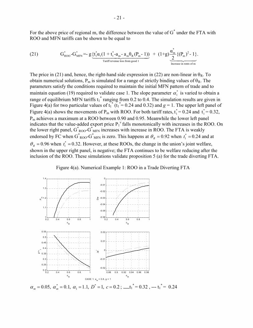
For the above price of regional m, the difference between the value of G* under the FTA with ROO and MFN tariffs can be shown to be equal to

(21) *

* * * * 2mROO MFN 1 1 1 m m R m m

Tariff revenue loss from good 1Increase in rents of m

αG -G =- g{t α (1 + t -a - a θ (P - 1)) + (1+g) {(P ) - 1}.214444424444431442443

The price in (21) and, hence, the right-hand side expression in (22) are non-linear in θR. To obtain numerical solutions, Pm is simulated for a range of strictly binding values of θR. The parameters satisfy the conditions required to maintain the initial MFN pattern of trade and to maintain equation (19) required to validate case 1. The slope parameter *

1α is varied to obtain a range of equilibrium MFN tariffs t1

* ranging from 0.2 to 0.4. The simulation results are given in Figure 4(a) for two particular values of t1* (t1

*= 0.24 and 0.32) and g = 1. The upper left panel of Figure 4(a) shows the movements of Pm with ROO. For both tariff rates, *

1t = 0.24 and *1t = 0.32,

Pm achieves a maximum at a ROO between 0.90 and 0.95. Meanwhile the lower left panel indicates that the value-added export price P1

v falls monotonically with increases in the ROO. On the lower right panel, G*

ROO-G*MFN increases with increase in ROO. The FTA is weakly

endorsed by FC when G*ROO-G*

MFN is zero. This happens at Rθ = 0.92 when *1t = 0.24 and at

Rθ = 0.96 when *1t = 0.32. However, at these ROOs, the change in the union’s joint welfare,

shown in the upper right panel, is negative; the FTA continues to be welfare reducing after the inclusion of the ROO. These simulations validate proposition 5 (a) for the trade diverting FTA.

Figure 4(a). Numerical Example 1: ROO in a Trade Diverting FTA

0.2 0.4 0.6 0.8 11

1.1

1.2

1.3

1.4

Pm

θR

0.2 0.4 0.6 0.8 10.2

0.25

0.3

0.35

0.4

0.45

0.5

0.55

Pv * 1

θR

0.2 0.4 0.6 0.8 1-0.06

-0.05

-0.04

-0.03

-0.02

-0.01

0

Dw

θR

0.88 0.9 0.92 0.94 0.96 0.98

-0.02

-0.01

0

0.01

0.02

Jp*

θRCASE 1: am = 0.8, g = 1

* *10.05, 0.1, 1.1, 1, 0.2m m D cα α α= = = = = ; t1

* = 0.32 , --- t1* = 0.24

- 22 -

Case 2Purely Trade Creating Case. This purely trade creating case requires that the total, within union supply in the FTA equilibrium without ROO be equal to the total demand of the FC. For the assumed demand and supply curves, this condition implies: (22) * * e

1 m 1 mD - c = α (1- a ) + γ α (1- a ) , where γe is as defined in Section IV. This FTA is welfare improving for FC and has no effect on the welfare of HC. Being purely trade creating in the absence of a ROO, the FTA necessarily improves joint welfare. In HC, the FTA leaves the value of G unchanged so that it weakly accepts the FTA. However, in FC, the reduction in the price of good 1 can lower the value of G* by lowering the return on

*1K .

Consider now the FTA in the presence of a ROO. Initially, a binding ROO increases the input price, which in turn, raises the price of good 1 faced by consumers in FC. All parameter values are maintained at the same values as under case 1 except 1α , which is assigned a higher value to ensure higher export capacity of good 1 in conformity with equation (22). It is verified that for the assumed values of the parameters, the value of G* under the FTA without ROO is less than that under MFN tariffs. The three equations determining * e

m 1P , P and γ are given by:

(23) e1m R m m*

m m

αP = θ γ a (1- a )α +α

,

(24) *

1 m R mP = 1 + a θ (P - 1) , and

(25) * * * *

e 1 1 1 m

1 m

(D - cP ) - α (P - a )γ = α (1- a )

.

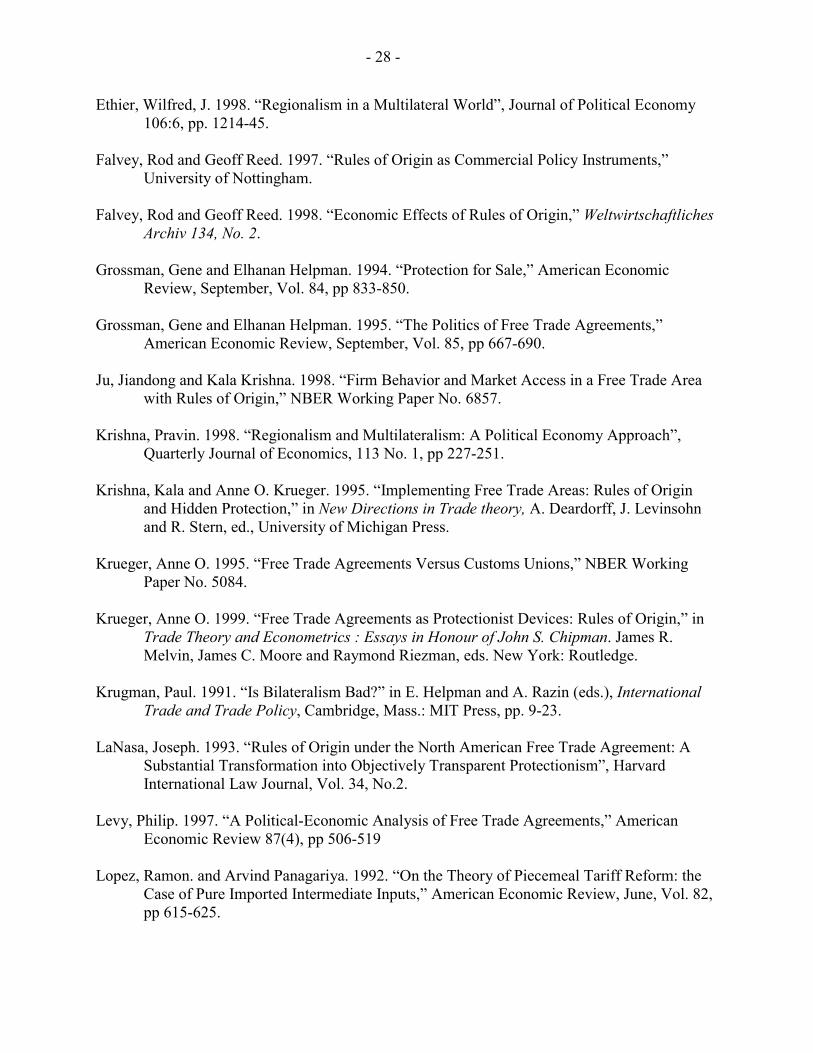
The results of the simulation are given in Figure 4(b). Note that G*

ROO- G*MFN is strictly positive

for all ROOs, implying that the FTA is unambiguously endorsed by FC. Also notice, that the price of good 1 in FC, P1

*, increases monotonically with the increase in the stringency of the ROO. If the ROO is such that Rθ ≤ 0.35, then joint welfare improves with the FTA. However,

- 23 -

for Rθ 0.35> , the ROO is so distortionary that joint welfare of the union actually falls with the FTA.26 These simulations validate proposition 5 (b) for the trade creating FTA.

Figure 4(b). Numerical Example 2: ROO in a Trade Creating FTA

0.34 0 .345 0.35 0.355

1.34

1.36

1.38

1.4

1.42

Pm

θR

0.377 0.378 0.379 0.38 0.381 0.382

1.14

1.145

1.15

1.155

1.16

P* 1

θR

0.2 0.3 0.4 0.5-0.06

-0.04

-0.02

0

0.02

DU

J

θR

0.25 0.3 0.350.005

0.01

0.015

0.02

G* R

OO

-G* M

FN

θR

CA S E 2, am = 0 .8, g = 1

* *

10.05, 0.1, 3.5, 1, 0.2m m D cα α α= = = = = , t1* = 0.24 , --- t1

* = 0.32

C. Extensions

The above analysis showed that a ROO could increase the viability of FTAs by facilitating the exchange of a tariff on a final good for a higher regional price on the intermediate input. However, ROOs could play a wider role in FTAs where positive tariffs exist on more than one final good, or when the political game determining the tariff structures is different. Without going into explicit analysis, three interesting extensions to the above model are discussed, which confirm that under different economic settings, ROOs could affect the viability of FTAs in different ways.

26 This is an important caveat to bear in mind for FTAs like the North American Free Trade Agreement (NAFTA) where the value-added ROOs in most sectors are typically between 0.50 and 0.625.

- 24 -

Extension 1. Both HC and FC Import Good 2 Suppose that both HC and FC import good 2 from ROW in the pre-FTA equilibrium (see Figure 1 again). Consider first the case without ROO on good 1 and assume t2 < t2

*.27 In this case, the producers of good 2 in HC export all production to FC after the FTA and consumption of good 2 in HC is met through imports. It can be verified (from equation (6)) that the HC continues to benefit from the FTA, and that FC’s payoff from FTA is worse than in the MFN equilibrium, implying that the FTA is infeasible in the absence of rules of origin (since it is rejected by FC). In the presence of ROO on the use of input m, FC may accept the ROO if the deficit in FC’s payoff as a result of loss in tariff revenue from goods 1 and 2 is more than compensated by the gain from the increase in producers’ surplus in good m. Again, the inclusion of ROO could increase the viability of the FTA. Now assume that t2

*< t2. In the absence of ROO, the FTA may or may not be accepted by both HC and FC given that HC (FC) loses tariff revenue in good 2 (good 1), and enjoys higher producer’s profits in good 1 (good 2). Suppose that both governments marginally accepted the FTA, i.e., the loss in HC’s payoff owing to tariff revenue loss from good 2 is exactly compensated by the gain in HC’s payoff as a result of increase in producers’ surplus in good 1, and analogously for FC. Next consider the FTA with a binding ROO. The negative impact of tariff revenue loss from good 1 is now lesser for FC (since a binding ROO would reduce the payoff for the exporters of good 1 from HC and hence their exports to FC) and more than compensated by the gain from producers’ surplus in good 2 and good m. However, this also implies that the gain in producer’s surplus from good 1 in HC is lesser (although HC also yields positive payoff from the producers’ surplus in good m). Thus, the FTA would continue to be viable only if the sum of the producers’ surplus from good 1 and input m in HC compensates for the loss in tariff revenue from good 2. If the losses outweigh the gains, HC would vote against the FTA. Thus, the FTA that is feasible in the absence of ROOs would then become infeasible once the ROOs are included. Extension 2. Endogenous determination of external tariffs in the post FTA equilibrium Suppose that the union members endogenously determine their external tariffs in the post FTA equilibrium and consider the post FTA equilibrium in the absence of ROO. Assume that ROW continues to export good 1 to FC after the FTA.28 Using the same payoff function as in Equation (6), the “optimal” external tariff on good 1 for the FC government would now be lower than that prior to the pre-FTA equilibrium.29 Since the FTA price of good 1 in FC is lower, the FTA 27 Also assume that the ROW continues to export goods 1 and 2 to the union in the post FTA equilibrium, such that the prices of good 1 is 1+ t1

* and that of good 2 is 1+ t2* (if t2 < t2

*) or 1+ t2 (if t2

* < t2) in the post FTA equilibrium.

28 Good 2 is eliminated from the analysis again.

29 It is also assumed that in determining external tariffs, FC takes the export supply from HC as exogenously given.

- 25 -

increases consumer surplus in FC at the cost of lowering producer’s surplus. Tariff revenue in the post FTA might also be greater, provided the increase in imports from ROW compensates the fall in external tariff rate. Thus, the FC’s decision to accept or reject the FTA becomes ambiguous depending on the relative weights given to the payoffs of alternative economic agents. Now consider the post FTA equilibrium in the presence of the ROO. A binding ROO would decrease the export supply from HC, thus increasing FC’s import and tariff revenue from the ROW. Again, a FTA that was rejected before might be accepted by the FC. Other interesting outcomes are also possible, such that a previously feasible FTA becomes infeasible in the presence of the ROO (e.g., if the shortfall in the producer’s surplus gain in good 1 in HC in the presence of ROO is greater than the producer’s surplus gain in input m). Extension 3. Exogenously given positive tariffs on final good and intermediate input Suppose that under the MFN equilibrium, the tariffs on goods 1 and m were t1 and tm, with tm > 0 and consider again the prospects of an FTA between HC and FC in the absence of ROOs given that ROW continues to export good 1 to FC after the FTA. Under the FTA, the loss in tariff revenue in good 1 (input m) for FC (HC) is partially or fully offset by the gain in producer’s surplus in input m (good 1). In the absence of ROOs, the FTA may or may not be feasible. Suppose that the FTA in the absence of the ROO is weakly feasible for both HC and FC. Now consider the political feasibility of the FTA in the presence of ROO. Starting from any given ROO and assuming that the ROO is not binding in that the FTA price of m is 1+tm, as the ROO becomes tighter, HC shifts its purchase of m from the ROW to FC and the loss in tariff revenue from good m for HC becomes larger. Thus, the inclusion of the ROO would actually make HC worse off and it would vote against the FTA, since HC was weakly endorsing the FTA in the absence of ROO. On the other hand, if the ROO is binding (Pm > 1+ tm), then even though the HC loses the entire tariff revenue on m, it benefits from greater producers’ surplus in input m, which enjoys a greater weight in the HC’s payoff relative to tariff revenue. In this situation, provided the gains outweigh the losses, the HC might continue to support the FTA.

VI. CONCLUSION

This paper offers an analysis of the relationship among traded intermediate inputs, rules of origin, welfare and political feasibility of FTAs. Our main results may be summarized as follows. First, contrary to the general impression in the policy literature, a ROO may improve or worsen the joint welfare of the union. Second, the price distortion created by the ROO has a direct bearing on the political economy of the FTA endorsement. By increasing rents for the interest group that owns the intermediate input, the ROO strengthens their potential influence on the government. Therefore there are situations when a member that unambiguously votes against the FTA in the absence of ROO would switch its vote in its presence. Finally and most importantly, the paper addresses the social desirability of an FTA that becomes feasible after the inclusion of a ROO. Two results are offered that have potentially important policy implications. One, an initially infeasible but welfare-reducing FTA becomes feasible after the inclusion of the ROO. And two, an infeasible but joint welfare improving FTA becomes

- 26 -

feasible upon ROO inclusion. However, the ROO can be so distortionary that after including its inclusion, the FTA becomes joint welfare diminishing. The paper provides insight into the politics behind the widespread use of product specific ROOs in the FTAs. For instance, the successful lobbying for strict ROO by the auto parts manufacturers in the United States under NAFTA did increase the trade in auto parts between Mexico and the United States. Similarly, the yarn forward rule directing trade in textiles in the NAFTA virtually amounting to a 100 percent value-added ROOhas played a crucial role in the phenomenal expansion of the U.S-Mexican trade in textiles.30 As shown in this paper, ROOs that protect domestic import competing industries as well as intermediate exporting industries can improve the chances of FTA endorsement for the country exporting inputs and importing final goods. However, the paper also shows that the FTA that is supported by stringent ROOs may not be desirable, as Anne Krueger has often argued. In conclusion, while the size of the ROO is treated as exogenous in this paper, the ROO can itself be subject to industry specific lobbying as evident from the experiences of the automotive parts, electronics, and textiles sectors under NAFTA. This feature can be incorporated into the analysis of the paper along the lines of the exclusion of sensitive sectors in Grossman and Helpman (1995). In view of the space constraints, we leave this extension to a future paper.

30 See Joseph A. LaNasa (1993) for an analysis of the restrictive nature of ROOs under the NAFTA.

- 27 -

REFERENCES

Andriamananjara Soamiley. 1999. “On the Size and Number of Regional Integration Arrangements: A Political Economy Model,” University of Maryland, mimeo.

Bagwell, Kyle and Robert W. Staiger. 1997a. “Multilateral Tariff Cooperation During the

Formation of Free Trade Areas,” International. Economic Review, 38:2, May, pp. 291-319.

Bagwell, Kyle and Robert Staiger. 1997b. “Multilateral Tariff Cooperation During the Formation

of Customs Unions,” Journal of International Economics 42:1-2, pp. 91-123. Baldwin, Richard. 1995. “A Domino Theory of Regionalism” in Expanding Membership of the

European Union. Richard Baldwin, P. Haaparnata, and J. Kiander, eds. Cambridge, U.K: Cambridge University Press, pp. 25-53.

Bernheim, FC. Douglas and Michael D. Whinston. 1986. “Menu Auctions, Resource allocation,

and Economic Influence.” Quarterly Journal of Economics, 101(1), pp 1-31. Bhagwati, Jagdish. 1993. “Regionalism and Multilateralism: An Overview,” in New Dimensions

in Regional Integration. Jaime de Melo and Arvind Panagariya, eds. pp. 22-51 Bhagwati, Jagdish, Pravin Krishna and Arvind Panagariya, eds. 1999. Trading Blocs:

Alternative Approaches to Analyzing Preferential Trade Agreements, Cambridge, MA: MIT Press.

Bhagwati, Jagdish and Arvind Panagariya. 1996. “The Theory of Preferential Trade Agreements:

Historical Evolution and Current Trends.” American Economics Review 86:2, pp. 82-87. Bond, Eric W. and Constantinos Syropoulos. 1996. “The Size of Trading Blocs, Market Power

and World Welfare Effects,” Journal of International Economics. 40:3-4, pp. 411-437. Cadot, Olivier, Jaime de Melo and Marcelo Olarreaga, 1999. "Regional Integration and

Lobbying for Tariffs Against Non-Members," Int. Econ. Rev. 40(3), 635-57. Cadot, Olivier, Jaime de Melo and Marcelo Olarreaga, 2000. “Can Duty-Drawbacks Have a

Protectionist Bias? Evidence from Mercosur,” Deardorff, Alan and Robert Stern. 1994. "Multilateral Trade Negotiations and Preferential

Trading Arrangements," in Analytical and Negotiating Issues in the Global Trading System. Alan Deardorff and Robert Stern, eds. Ann Arbor, MI: University of Michigan Press, pp. 53-85.

Duttagupta, Rupa. 2000. “Intermediate Inputs and Rules of Origin: Implications for Welfare and

Viability of Free Trade Agreements”, University of Maryland, Ph.D. Thesis.

- 28 -

Ethier, Wilfred, J. 1998. “Regionalism in a Multilateral World”, Journal of Political Economy 106:6, pp. 1214-45.

Falvey, Rod and Geoff Reed. 1997. “Rules of Origin as Commercial Policy Instruments,”

University of Nottingham. Falvey, Rod and Geoff Reed. 1998. “Economic Effects of Rules of Origin,” Weltwirtschaftliches

Archiv 134, No. 2. Grossman, Gene and Elhanan Helpman. 1994. “Protection for Sale,” American Economic

Review, September, Vol. 84, pp 833-850. Grossman, Gene and Elhanan Helpman. 1995. “The Politics of Free Trade Agreements,”

American Economic Review, September, Vol. 85, pp 667-690. Ju, Jiandong and Kala Krishna. 1998. “Firm Behavior and Market Access in a Free Trade Area

with Rules of Origin,” NBER Working Paper No. 6857. Krishna, Pravin. 1998. “Regionalism and Multilateralism: A Political Economy Approach”,

Quarterly Journal of Economics, 113 No. 1, pp 227-251. Krishna, Kala and Anne O. Krueger. 1995. “Implementing Free Trade Areas: Rules of Origin

and Hidden Protection,” in New Directions in Trade theory, A. Deardorff, J. Levinsohn and R. Stern, ed., University of Michigan Press.

Krueger, Anne O. 1995. “Free Trade Agreements Versus Customs Unions,” NBER Working

Paper No. 5084. Krueger, Anne O. 1999. “Free Trade Agreements as Protectionist Devices: Rules of Origin,” in

Trade Theory and Econometrics : Essays in Honour of John S. Chipman. James R. Melvin, James C. Moore and Raymond Riezman, eds. New York: Routledge.

Krugman, Paul. 1991. “Is Bilateralism Bad?” in E. Helpman and A. Razin (eds.), International

Trade and Trade Policy, Cambridge, Mass.: MIT Press, pp. 9-23. LaNasa, Joseph. 1993. “Rules of Origin under the North American Free Trade Agreement: A

Substantial Transformation into Objectively Transparent Protectionism”, Harvard International Law Journal, Vol. 34, No.2.

Levy, Philip. 1997. “A Political-Economic Analysis of Free Trade Agreements,” American

Economic Review 87(4), pp 506-519 Lopez, Ramon. and Arvind Panagariya. 1992. “On the Theory of Piecemeal Tariff Reform: the

Case of Pure Imported Intermediate Inputs,” American Economic Review, June, Vol. 82, pp 615-625.

- 29 -

Olson, Mancur. 1965. “The Logic of Collective Action”, Cambridge, MA: Harvard University Press.

Panagariya, Arvind. 1999. “The Regionalism Debate: An Overview,” World Economy 22, 477-

511. Panagariya, Arvind. 1999. “Preferential Trading and Welfare: The Small-Union Case Revisited”,

University of Maryland (unpublished). Panagariya, Arvind. 2000. “Preferential Trade Liberalization: The Traditional Theory and new

Developments”, Journal of Economic Literature XXXVIII, 287-331. Panagariya, Arvind and Ronald Findlay. 1996. “A Political Economy Analysis of Free Trade

Areas and Customs Unions,” in Robert Feenstra, Gene Grossman, and Douglas Irwin, eds., The Political Economy of Trade Reform, essays in honor of Jagdish Bhagwati, MIT Press, 1996.

Reproduced as Chapter 17 in Bhagwati, J., P. Krishna and Arvind Panagariya, eds., Trading

Blocs: Alternative Approaches to Analyzing Preferential Trade Agreements, Cambridge, MA: MIT Press, February 1999.

Panagariya, Arvind and Pravin Krishna. (forthcoming). “On Welfare Enhancing FTAs,” Journal

of International Economics. Srinivasan, T.N. 1993. “Regionalism versus Multilateralism: Analytical Notes. Comment,” in

New Dimensions in Regional Integration, Jaime de Melo and Arvind Panagariya eds. Cambridge, Great Britain: Cambridge University Press, pp. 84-89.

Viner, Jacob. 1950. The Customs Union Issue. New York: Carnegie Endowment for International

Peace. Yi, Sang-Seung. 1996. “Endogenous Formation of Customs Unions under Imperfect

Competition: Open Regionalism is Good,” Journal of International Economics. 41:1-2, pp. 153-77.