1

Free book on Eddy covariance. Nicely produced by the company that produces many of the top instruments for eddy covariance and who has invested in producing open access software, EddyPro, for data logging and producing fluxes. http://www.licor.com/env/products/eddy_covariance/software.html

Both Burba and I were students of Shashi Verma, so we had lessons from the pioneer.  Parts of this book are taken from this course, but produced much nicer, so it is a great reference to add to your book shelf.

http://www.licor.com/env/products/eddy_covariance/ec_book.html

2

Aubinet et al is a real nice paper and one of the early reviews on eddy covariance, as written for documentation for the EuroFlux community. I think it is important that you read independent papers from me to get alternative perspectives

But for background, it may be worthwhile to read one of my reviews, too, since I am an expert on this topic.  My paper is widely used and is a follow up from a 1988 paper I wrote for Ecology with Bruce Hicks and Tilden Meyers.  This GCB paper has an interesting history, worth recounting. It was written on commission for the Annual Reviews of Ecology and Systematics, circa 2001‐02.  After about 10 months I had heard nothing and was starting to see papers printed for the volume this paper was intended.  I wrote the editor and found out he had lost track of the paper…he then got a hasty review by a card carrying ecologist who recommended rejection because they did not understand it; I had had the paper vetted by expert peers, so I knew this was wrong.  Hence, I withdrew the paper and I wrote to Steve Long, editor at Global Change Biology, who encouraged me to submit the paper.  Well long story short, the paper has been successful.  Steve Long recently wrote to inform me it is one of the top cited papers in the 20 year history of GCB.  So this is a lesson in perseverance and persistence…and realizing some editors can be wrong (a confession, written by the editor in chief of JGR. Biogeosciences).

3

The first and earliest papers go back to work by F. J. Scrase 1930 Some characteristics of eddy motion in the atmosphere. Only a few studies were conducted in the 1970s and 80s, with active groups including Verma at Nebraska, Hicks and Wesely at Argonne, Denmead at CSIRO in Australia, Desjardins Ag Canada, Ohtaki in Japan, the NCAR group of Lenschow, Wyngaard and Kaimal, David Fowler, Jim Shuttleworth at Center for Ecology and Hydrology (near Edinburghand Wallingford, UK), Jenson and colleagues at RISO in Denmark (life was simpler as there were fewer papers to track and you could count the groups active on both hands).

The field is rather new and the explosion in its use has trended with the PC and the availability of a affordable and robust computation and data storage.  Big field studies like Fife and Boreas in the late 80s and early 90s also stimulated growth in the field as scientists were becoming more confident in making eddy covariance flux measurements unattended.  In the 80’s we literally were in the field for each hour of data we collected, changing disc drives, calibrating, fixing problems, covering instruments in the event of rain. And my former NOAA/ATDD group was one of the first to mass produce open path CO2/water vapor sensors that were stable and affordable (Auble and Meyers), which then lead to independent commercialization of a very high quality sensor by LICOR and who produced software that could be shared and used for data acquisition (see McMillen et al).

4

These are the compelling reasons why people like me are adherents and advocates of the eddy covariance method. It measures fluxes of the complex systems people want to measure, yet have difficulty doing so with sets of chambers, deployed manually

5

The equation for eddy covariance is deceptively simple.  It is the covariance between fluctuations in vertical velocity, w’, and mixing ratio, s.

Because we separate fluctuation from the means, the excessive accuracyrequirements needed to make gradient measurements is relaxed.

6

Ideally it is preferable to define F in terms of mixing ratio, the ratio of partial pressures, that define concentrations.  One of the first complications we will see is that few if any sensors measure mixing ratio, so more terms will need to be considered

7

The key to evaluating the eddy covariance is that we need to measure all the fast and slow fluctuations that occur in the turbulent atmosphere. Here is a time series showing the turbulent flucuations in vertical velocity and temperature.  Note coherent patterns of sustained updrafts and down drafts associated with parcels of warmer and cooler air.

8

Dialing in on the time series for periods of 24 hours, one hour and 100 seconds for vertical velocity. I love MATLAB. It has given me a whole new vision and appreciation of the dynamics of turbulent fluctuations over a day.  In the past we watch the computer screen but only saw 5 min windows of turbulence.  Processing data in Basic and C did not give us the opportunity to visual the data as we processed it.  With MATLAB we can visualize data in a variety of windows of time.  I’ll give you some raw data to play with in the next lecture or two and be creative and explore.

9

Dialing in on the time series for periods of 24 hours, one hour and 100 seconds for CO2. Note the coherent structures that transfer lots of material through sweeps and ejections.  Over 100s we may experience 8 to 10 such events.

10

The computation of the eddy covariance relies on computing the mean from a time series and the fluctuations of the mean.  The mean has to be long enough to capture the ensemble of low frequency, but important transfer events, yet not too long to introduce daily trends.

11

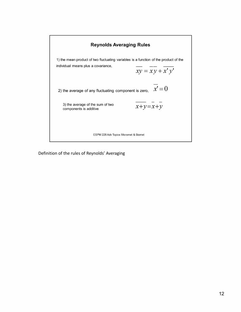
Definition of the rules of Reynolds’ Averaging

12

Let’s do the algebra to compute the eddy covariance from the mean mass flux as we have three time varying variables, density, vertical velocity and specific concentration of the scalar

13

14

15

16

17

18

19

20

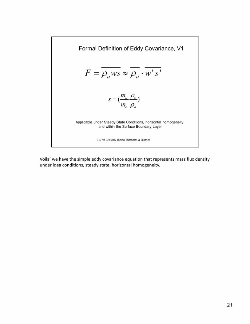
Voila’ we have the simple eddy covariance equation that represents mass flux density under idea conditions, steady state, horizontal homogeneity.

21

Beer’s law which is the basis behind infrared spectrometers, lyman alpha hygrometers and tunable diode laser spectrometers measures the mole density within the path in which light is absorbed by molecules of interest.  So in reality we don’t have instruments that measure s per se.

22

The LI 7500 is an open path sensor that can be placed close to the sonic anemometer to measure Co2 and H2O with minimal disturbance. The altnerative involves suck air down a tube to an analyzer. This requires power hungry pumps and is susceptible to fluctuation dampening as air interacts with tube walls.

23

Simplest case for dry air with fluctuations in temperature.  The mean vertical velocity is not exactly zero.  It is a very small but non zero value and since it is multiplied by a large quantity, this product can produce a sizeable flux density that is added, or subtracted from the formal covariance.

24

Why is w non zero?  We can inspect this cartoon for some perspective.  The density fluctuation theory laid out by Webb, Pearman and Leuning, indicates there is a small vertical velocity, too small to measure with a sonic anemometer, but large enough to bias the flux measurements and in many circumstances change the sign, or direction, of the flux!!  Changes in temperature, for example can alter the volume of a parcel of air, as can additional moisture through adding to the partial pressure of that volume.  So changes in pressure and temperature cause changes in volume, that cause expansion or contraction of the parcel, leading to a velocity, dx/dt

25

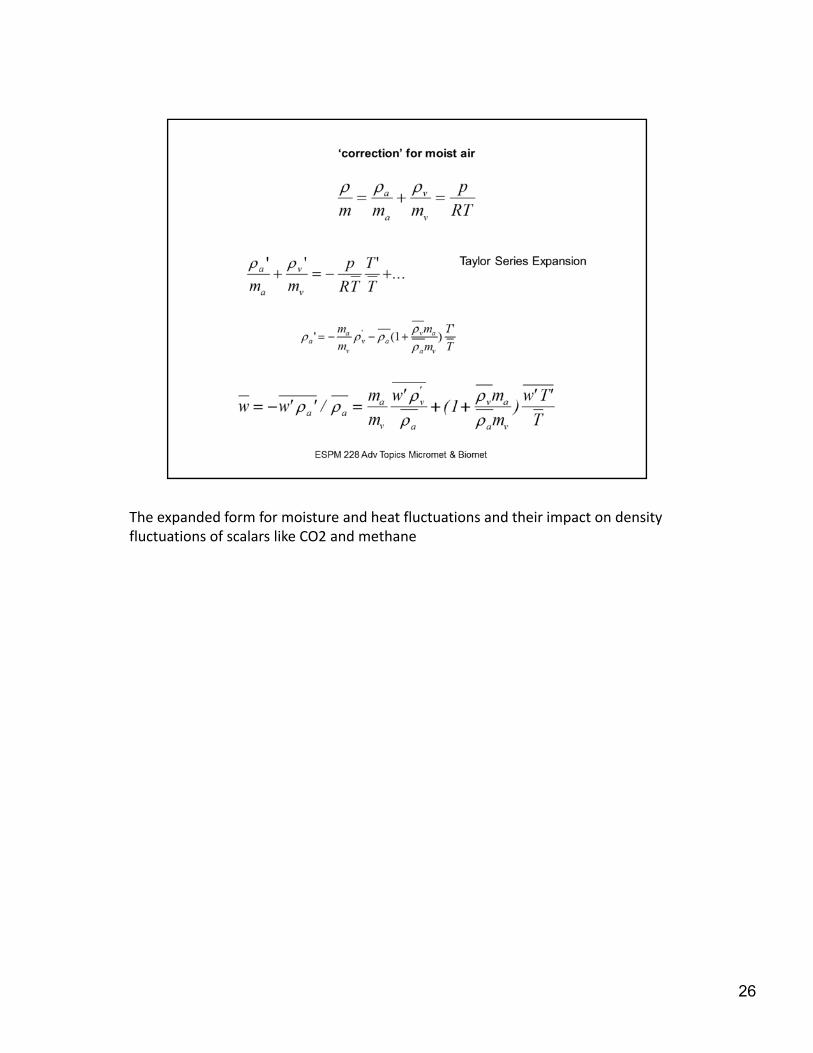
The expanded form for moisture and heat fluctuations and their impact on density fluctuations of scalars like CO2 and methane

26

This equation shows you must measure fluxes of moisture and heat when measuring fluxes of a trace gas

27

This figure shows the relative correction to the raw CO2 flux covariance with varyingvalues of H and LE.  Corrections are most severe with high values of sensible heat exchange

28

29

This figure gives an example why it is important to consider the wpl correction.  Under certain conditions the sign of the raw and ‘corrected’ flux density can be of opposite signs, especially when H, sensible heat exchange, is high, as when the forest is leafless and respiring, but the raw covariance suggests it is photosynthesizing.

30

This study proves the contention that the covariance measured with mixing ratio equals that computed with WPL with mole density measurements

31

Interesting case of a resistance to paradigm shift (see Thomas Kuhn, The Structure of Scientific Revolution).  There have been many attempts by young and ambitious scientists to overturn WPL.  Yet, in most circumstances the critics have been proven wrong and WPL theory has withstood independent tests.

It is my opinion that this theory is resistant to paradigm shifts because the theory is correct..the only term missing here is the role of pressure fluctuations, but they tend to be on the order of +/‐ 10 Pa in an atmosphere that is 101.3 kPa

32

One of the more clever studies, test of the WPL theory on the Kansas State Football Field Parking lot

33

At Cal we don’t have big parking lots like the Midwest Football schools.  So We did our own parking lot tests at Moffett Field, NASA Ames

34

During the summer at our annual grassland the raw fluxes infer photosynthesis, but the grass is dead. Only after wpl corrections are applied do we get the right sign.  Though I do remain skeptical about the magnitude of the day effluxes as the soil is so dry, yet it lead us to investigate the role of photodegradation,

35

36

The one big problem is the accuracy of open path CO2 flux measurements are a function of the accuracy of measurements of sensible and latent heat exchange.  Why may this be a problem?  There continues to be wide spread lack of energy balance closure with across eddy covariance flux sites.  In certain instances it may be due to filtering of the flux covariance measurements. Nevertheless, the lack of wide spread closure raises skepticism by critics of errors in the carbon balances we produce. And remember a bias error of only 1 micromol m‐2 s‐1 over a year can accumulate to 400 gC m‐2 y‐1.  So we want to remove all possible sources of errors..now are you appreciating how the deceptively simple covariance equation can become very complicated in practice?  And we are only at the tip of the ice berg on this topic. More is to come.

37

38

Even closed path sensors need some corrections for moisture.  Theory assumes that sampling through a tube dampens temperature fluctuations

39

40

Burba Corrections

41

In the cold and snow of the north there has been concerns about self heating of the sensor and causing some spurious corrections.  Grelle and Burba have worked hardon this problem.

42

The development of the LI 7200 is an optimal design that yields the benefits of the small, low power LI 7500 with the closed path attributes of minimizing temperature and rain problems that may plague the LI 7500 in wet environments

43

Ray Leuning, one of the wise men and pioneers of flux measurements has said it best. ‘Know thy site’.  When you start a new experiment at a new site do your due diligence and check for all the possible advection and storage effects, as well as other itemslike spectra, we will talk about later.

44

Eddy covariance measurements are typically made in the real world, where fetch is not infinite, fetch is heterogeneous, terrain is undulating or sloping and the atmosphere is not at steady state. So we have to think about the 3D budget equation and make measurements of other terms that may not be negligible.

In the following we will describe how we arrive at the assumption of a constant flux layer and the relation between flux densities, flux divergences and the conservation budget for a scalar, c.  This theoretical framework will guide us for using the eddy covariance method under ideal and less ideal situation. It will tell us what else to measure when we apply the eddy covariance method in less ideal conditions, because remember the real world is mostly non ideal.

45

We see and use this equation everywhere in environmental fluid mechanics, micrometeorology and biometeorology.  Understanding how these terms arise and which ones are negligible tell us about the constant flux layer and the impacts of advection and storage on interpreting eddy covariance measurements

46

We will dive into the 3 D budget equation. So start with a conceptual volume of air and consider how the scalar concentration changes with time as there are fluxes of material into and out of each face.

47

First lets look at what the total derivative dc/dt means.

48

We can break the partial derivative of the product (d [a b] /dx) using the product rule of derivatives d(a b)/dx = a db/dx + b da/dx

49

Consider the case of the budget of air density, rho

50

From the continuity equation, because air is considered incompressible for our situation, this budget sums to zero.

51

So we can drop the terms with du/dx + dv/dy +dw/dz. Now we are starting to see terms that are familiar if we go back to the master equation at the beginning of this section.

52

53

In this case we are assuming the budget with just diffusion.  We need to start with this basic instantaneous equation to derive the equation for turbulence

54

Starting with the simple diffusion budget we now apply rules of Reynolds’ averaging to define the conservation equation for turbulent flows.

The most important point is the introduction of a new term, d <u’c’>/dx..This is the turbulent flux divergence.

55

In turbulent flows the diffusive flux divergence is tiny and ignored.  So we now have the full fledged time averaged conservation budget in turbulent flow.

56

We can break up this equation into its terms, yielding information on time rate of change, advection and flux divergence

57

Under ideal conditions we assume steady state (dc/dt is zero) and infinite fetch so advection is zero (dc/dx = 0), yielding the vertical flux divergence equal zero (d <w’c’>/dz), which is the constant flux layer. It does not say the vertical flux is zero, just the flux divergence. Hence if we measure <w’c’> at a level z over the canopy we can be assured it equals the flux of material in and out of the canopy.!!!!!!

58

59

60

61

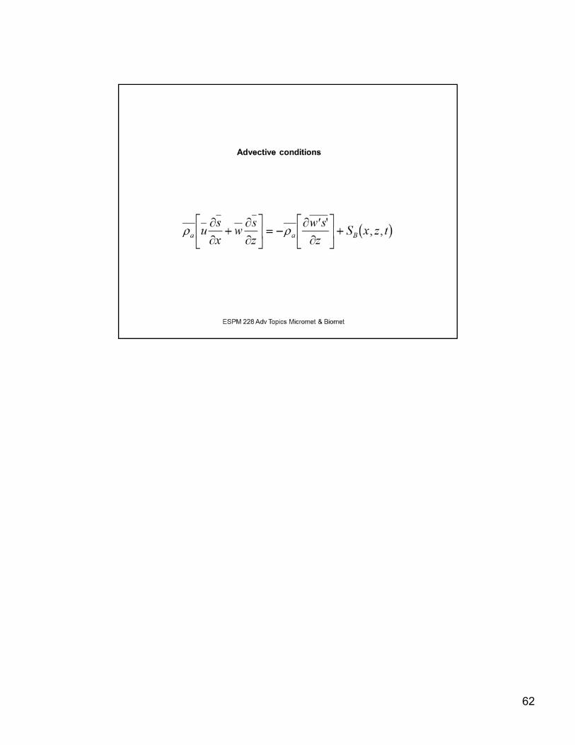
62

It is often difficult to measure the horizontal gradients needed to assess advection as wind direction changes. One idea is to measure flux gradients

63

Many interesting and important AmeriFlux/FLUXNET sites are on topographically challenging locations.  Here is the Niwot Ridge site operated by the team at University of Colorado, formerly under Russ Monson.

64

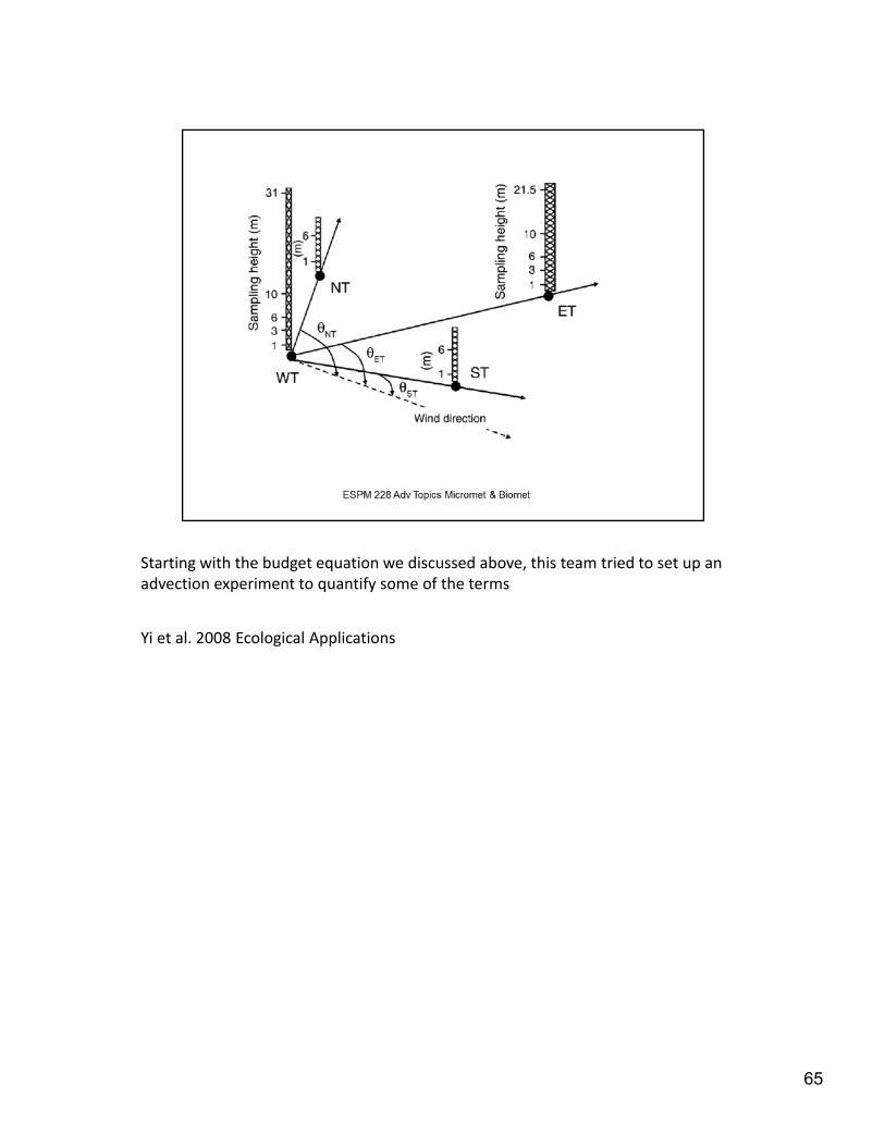
Starting with the budget equation we discussed above, this team tried to set up an advection experiment to quantify some of the terms

Yi et al. 2008 Ecological Applications

65

66

Missing different advection and storage terms in complex terrain can yield huge differences in the net annual carbon flux

Yi et al 2008 Ecological Applications

67

68

If you are to be an eddy flux practitioner or consumer of such data this lecture gives you the fundamentals!

69