Frank J. Wentz and Thomas MeissnerRemote Sensing Systems

Aquarius Salinity Algorithm and Simulations

Aquarius/SAC-D Science Workshop19-21 July 2010, Seattle WA

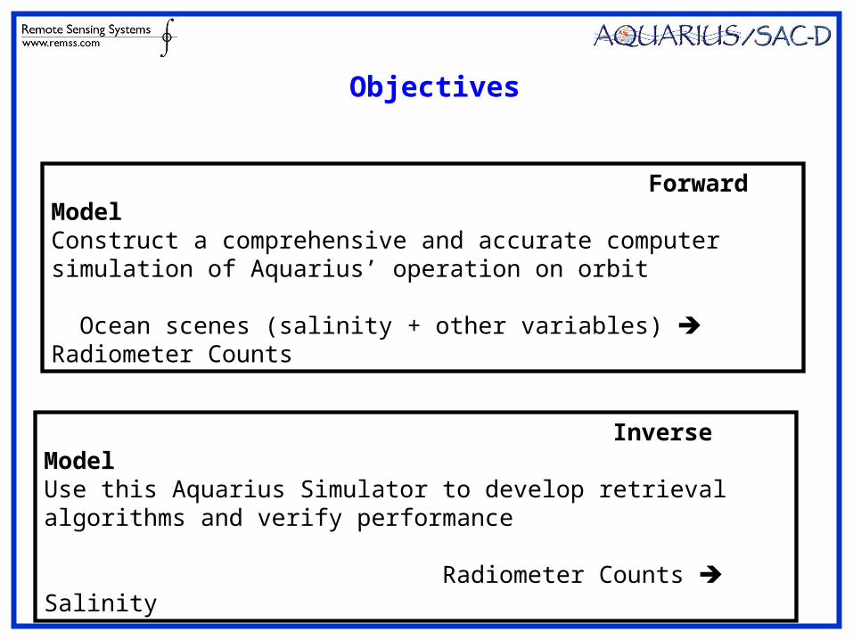
Objectives

Forward ModelConstruct a comprehensive and accurate computer simulation of Aquarius’ operation on orbit

Ocean scenes (salinity + other variables) Radiometer Counts

Inverse ModelUse this Aquarius Simulator to develop retrieval algorithms and verify performance

Radiometer Counts Salinity

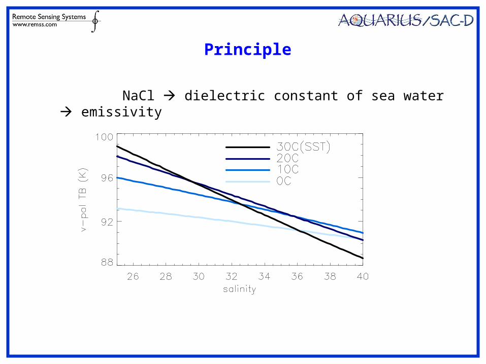
NaCl dielectric constant of sea water emissivity

Principle

Aquarius

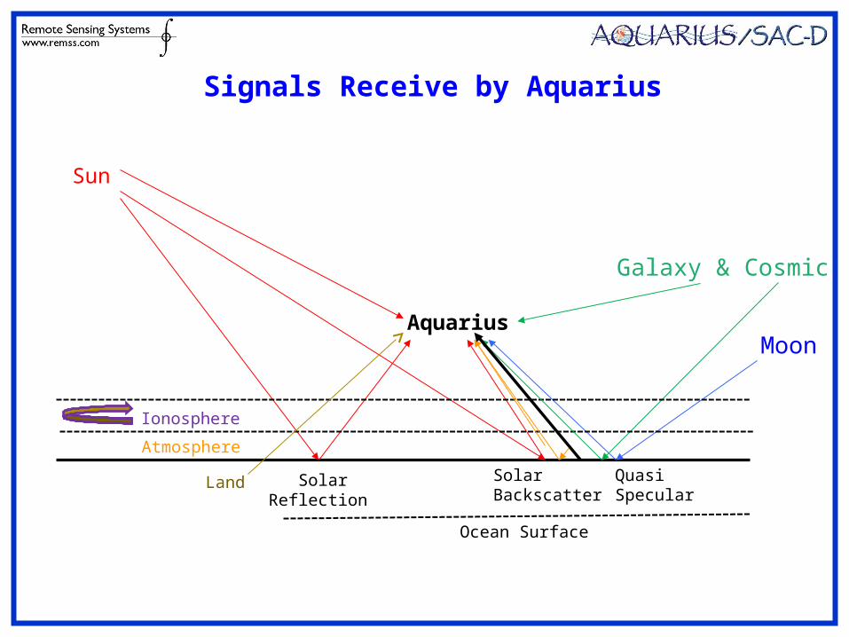
Sun

SolarReflection

QuasiSpecular

SolarBackscatter

Galaxy & Cosmic

Moon

Ocean Surface

Signals Receive by Aquarius

Ionosphere

Atmosphere

Land

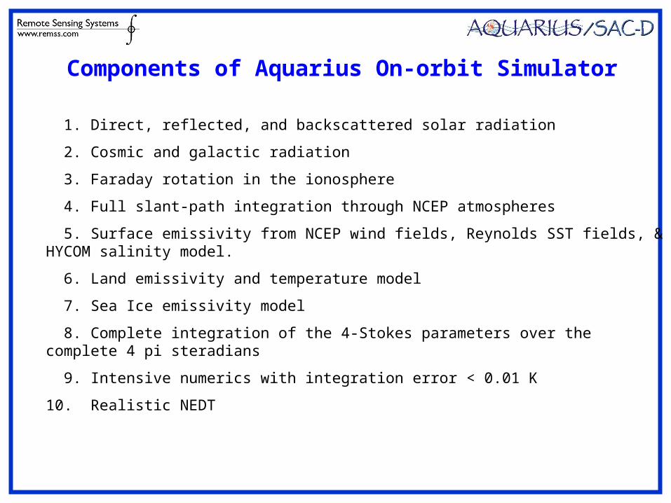
Components of Aquarius On-orbit Simulator

1. Direct, reflected, and backscattered solar radiation

2. Cosmic and galactic radiation

3. Faraday rotation in the ionosphere

4. Full slant-path integration through NCEP atmospheres

5. Surface emissivity from NCEP wind fields, Reynolds SST fields, & HYCOM salinity model.

6. Land emissivity and temperature model

7. Sea Ice emissivity model

8. Complete integration of the 4-Stokes parameters over the complete 4 pi steradians

9. Intensive numerics with integration error < 0.01 K

10. Realistic NEDT

, ,

, ,

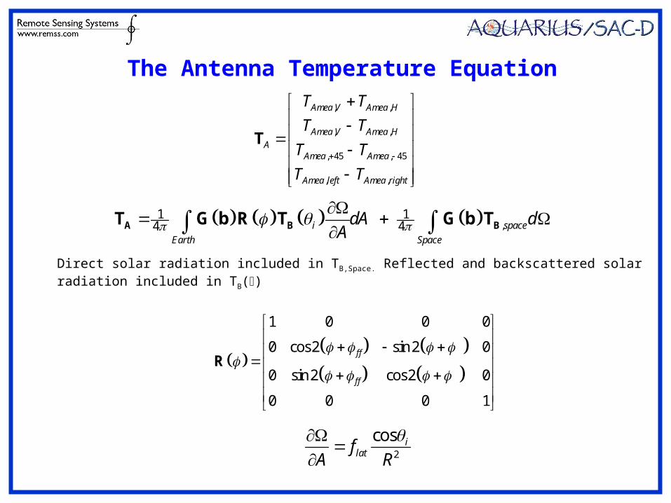
, 45 , 45

, ,

Amea V Amea H

Amea V Amea H

AAmea Amea

Amea left Amea right

T T

T T

T T

T T

T

,1 1

4 4i space

Earth Space

dA dA

A B BT G b R T G b T

1 0 0 0

0 cos2 sin 2 0

0 sin 2 cos2 0

0 0 0 1

f f

f f

R

2

cos ilatfA R

Direct solar radiation included in TB,Space. Reflected and backscattered solar radiation included in TB()

The Antenna Temperature Equation

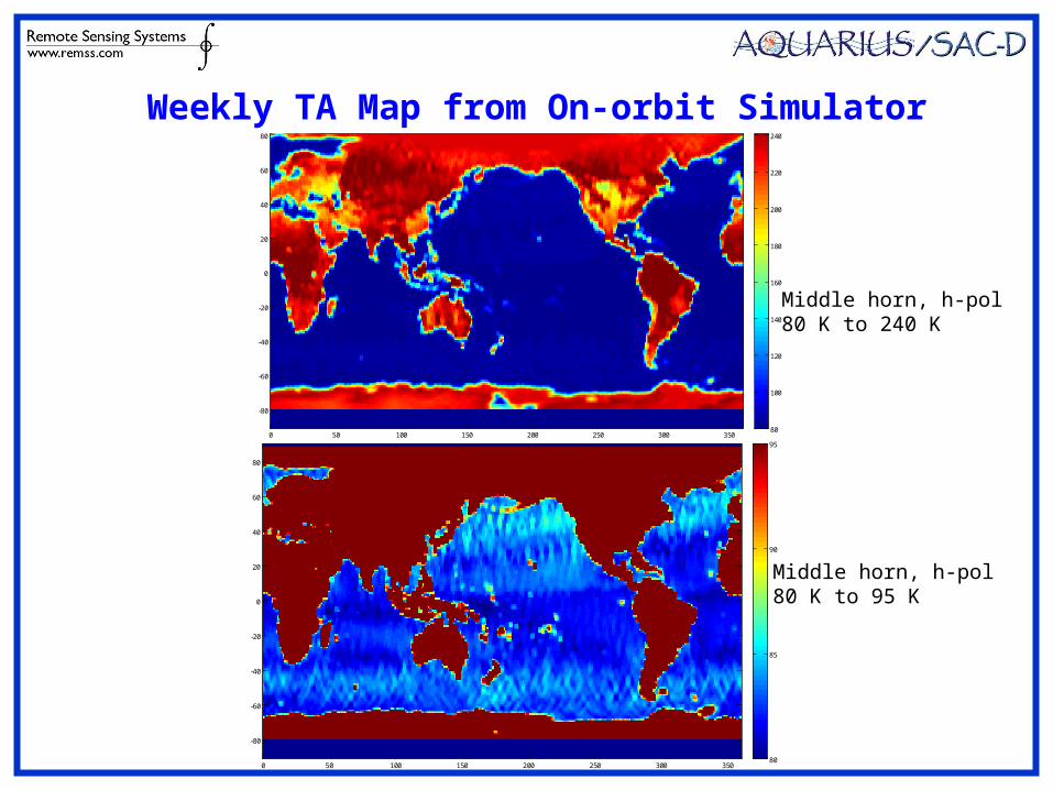
0 50 100 150 200 250 300 350

-80

-60

-40

-20

0

20

40

60

80

80

100

120

140

160

180

200

220

240

0 50 100 150 200 250 300 350

-80

-60

-40

-20

0

20

40

60

80

80

85

90

95

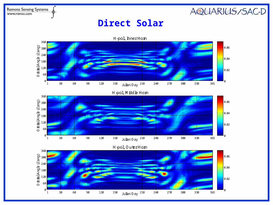
Weekly TA Map from On-orbit Simulator

Middle horn, h-pol80 K to 240 K

Middle horn, h-pol80 K to 95 K

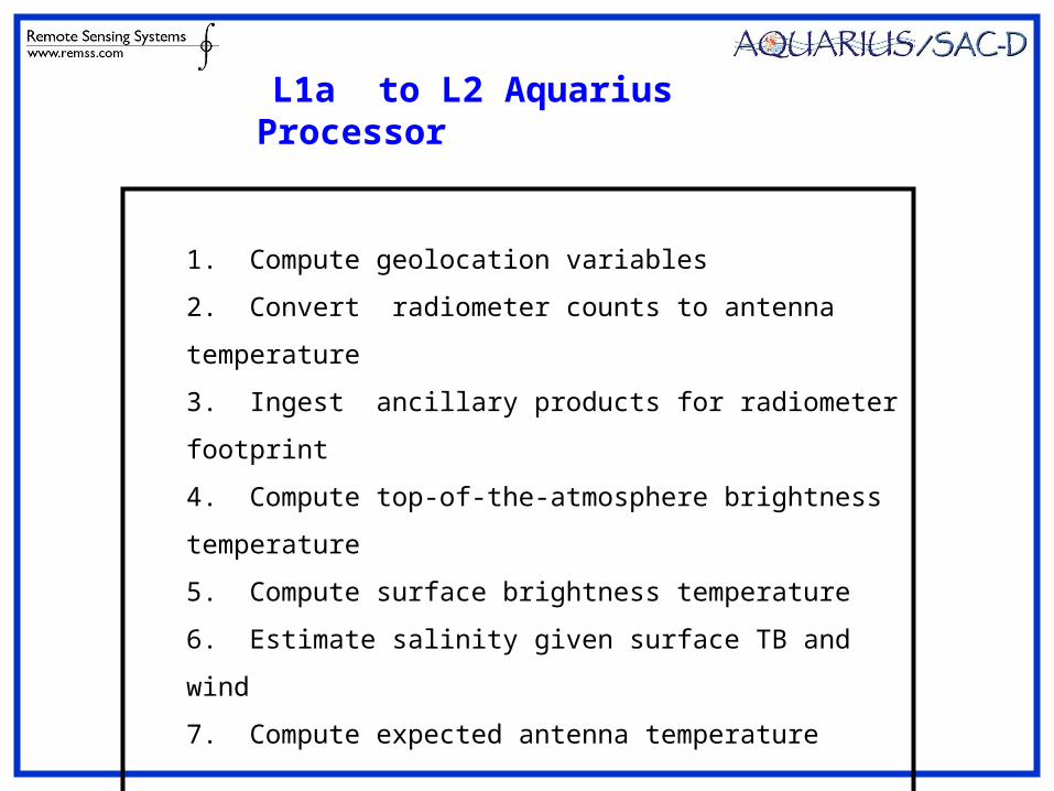
1. Compute geolocation variables

2. Convert radiometer counts to antenna temperature

3. Ingest ancillary products for radiometer footprint

4. Compute top-of-the-atmosphere brightness temperature

5. Compute surface brightness temperature

6. Estimate salinity given surface TB and wind

7. Compute expected antenna temperature

L1a to L2 Aquarius Processor

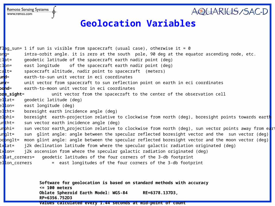
iflag_sun= 1 if sun is visible from spacecraft (usual case), otherwise it = 0zang= intra-orbit angle. it is zero at the south pole, 90 deg at the equator ascending node, etc.sclat= geodetic latitude of the spacecraft earth nadir point (deg)sclon= east longitude of the spacecraft earth nadir point (deg)scalt= spacecraft altitude, nadir point to spacecraft (meters)sund= earth-to-sun unit vector in eci coordinates sunr= unit vector from spacecraft to sun reflection point on earth in eci coordinatesmoond= earth-to-moon unit vector in eci coordinates bore_sight= unit vector from the spacecraft to the center of the observation cellcellat= geodetic latitude (deg)cellon= east longitude (deg)celtht= boresight earth incidence angle (deg)celphi= boresight earth-projection relative to clockwise from north (deg), boresight points towards earthsuntht= sun vector earth incidence angle (deg)sunphi= sun vector earth_projection relative to clockwise from north (deg), sun vector points away from earthsunglt= sun glint angle: angle between the specular reflected boresight vector and the sun vector (deg)mooonglt= moon glint angle: angle between the specular reflected boresight vector and the moon vector (deg)glxlat= j2k declination latitude from where the specular galactic radiation originated (deg)glxlon= j2k ascension from where the specular galactic radiation originated (deg)cellat_corners= geodetic latitudes of the four corners of the 3-db footprintcellon_corners= east longitudes of the four corners of the 3-db footprint

Geolocation Variables

Software for geolocation is based on standard methods with accuracy <= 100 metersOblate Spheroid Earth Model: WGS-84 RE=6378.137D3, RP=6356.752D3Values calculated every 1.44 seconds at mid-point of count averaging.

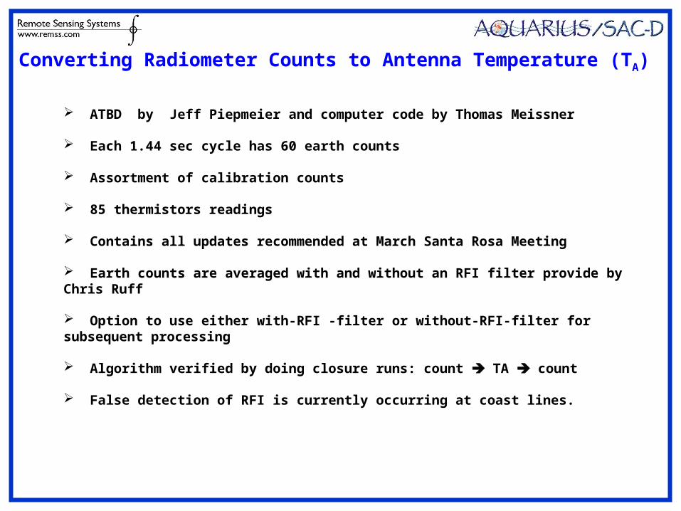
Converting Radiometer Counts to Antenna Temperature (TA)

ATBD by Jeff Piepmeier and computer code by Thomas Meissner

Each 1.44 sec cycle has 60 earth counts

Assortment of calibration counts

85 thermistors readings

Contains all updates recommended at March Santa Rosa Meeting

Earth counts are averaged with and without an RFI filter provide by Chris Ruff

Option to use either with-RFI -filter or without-RFI-filter for subsequent processing

Algorithm verified by doing closure runs: count TA count

False detection of RFI is currently occurring at coast lines.

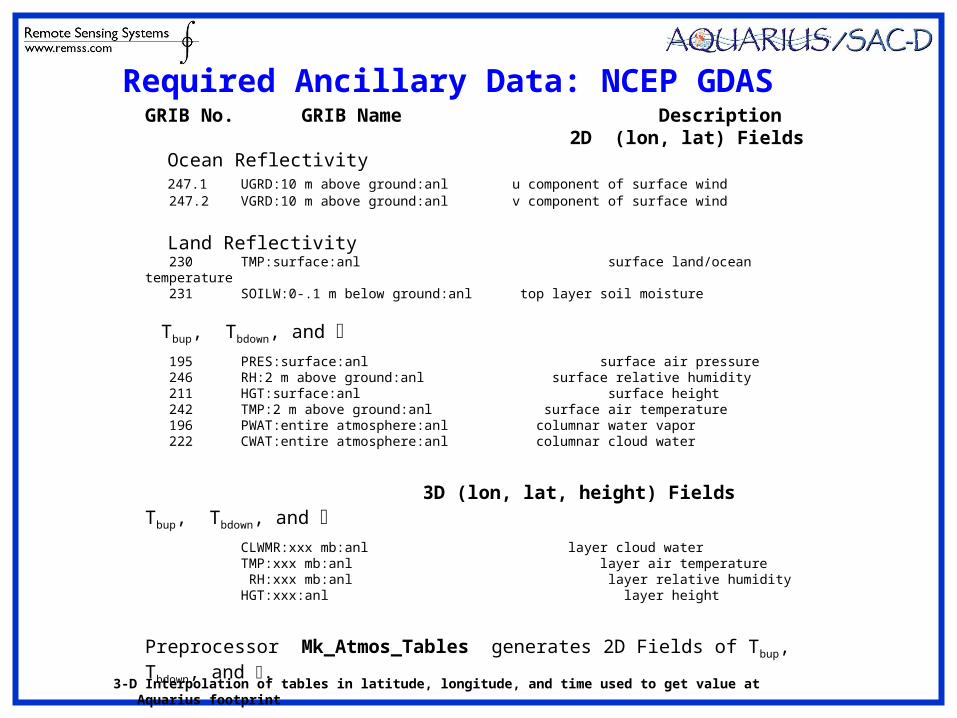
GRIB No. GRIB Name Description 2D (lon, lat) Fields Ocean Reflectivity 247.1 UGRD:10 m above ground:anl u component of surface wind 247.2 VGRD:10 m above ground:anl v component of surface wind

Land Reflectivity 230 TMP:surface:anl surface land/ocean temperature 231 SOILW:0-.1 m below ground:anl top layer soil moisture

Tbup, Tbdown, and 195 PRES:surface:anl surface air pressure 246 RH:2 m above ground:anl surface relative humidity 211 HGT:surface:anl surface height 242 TMP:2 m above ground:anl surface air temperature 196 PWAT:entire atmosphere:anl columnar water vapor 222 CWAT:entire atmosphere:anl columnar cloud water

3D (lon, lat, height) FieldsTbup, Tbdown, and

CLWMR:xxx mb:anl layer cloud water TMP:xxx mb:anl layer air temperature RH:xxx mb:anl layer relative humidity HGT:xxx:anl layer height

Preprocessor Mk_Atmos_Tables generates 2D Fields of Tbup, Tbdown, and .

Required Ancillary Data: NCEP GDAS

3-D Interpolation of tables in latitude, longitude, and time used to get value at Aquarius footprint

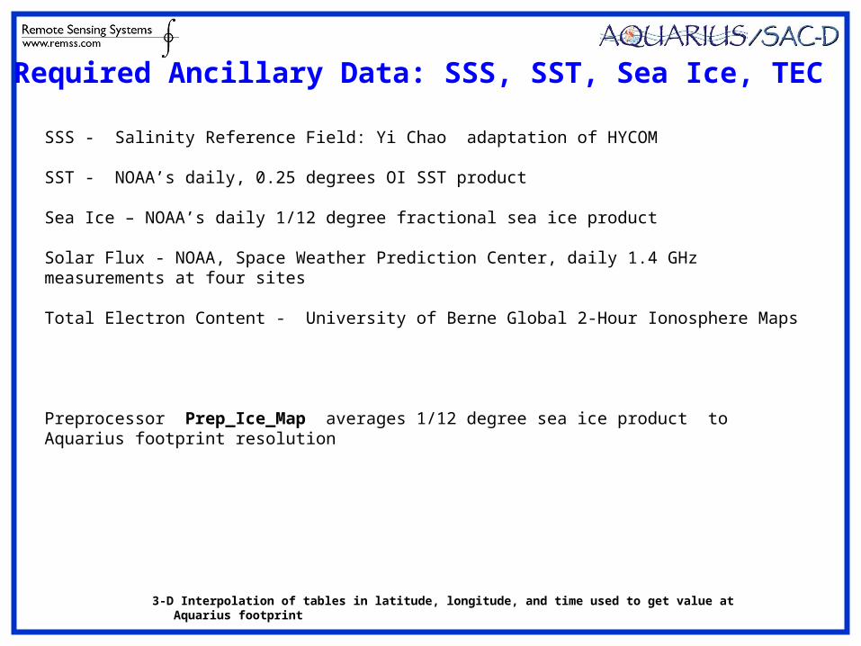
SSS - Salinity Reference Field: Yi Chao adaptation of HYCOM

SST - NOAA’s daily, 0.25 degrees OI SST product

Sea Ice – NOAA’s daily 1/12 degree fractional sea ice product

Solar Flux - NOAA, Space Weather Prediction Center, daily 1.4 GHz measurements at four sites

Total Electron Content - University of Berne Global 2-Hour Ionosphere Maps

Preprocessor Prep_Ice_Map averages 1/12 degree sea ice product to Aquarius footprint resolution

3-D Interpolation of tables in latitude, longitude, and time used to get value at Aquarius footprint

Required Ancillary Data: SSS, SST, Sea Ice, TEC

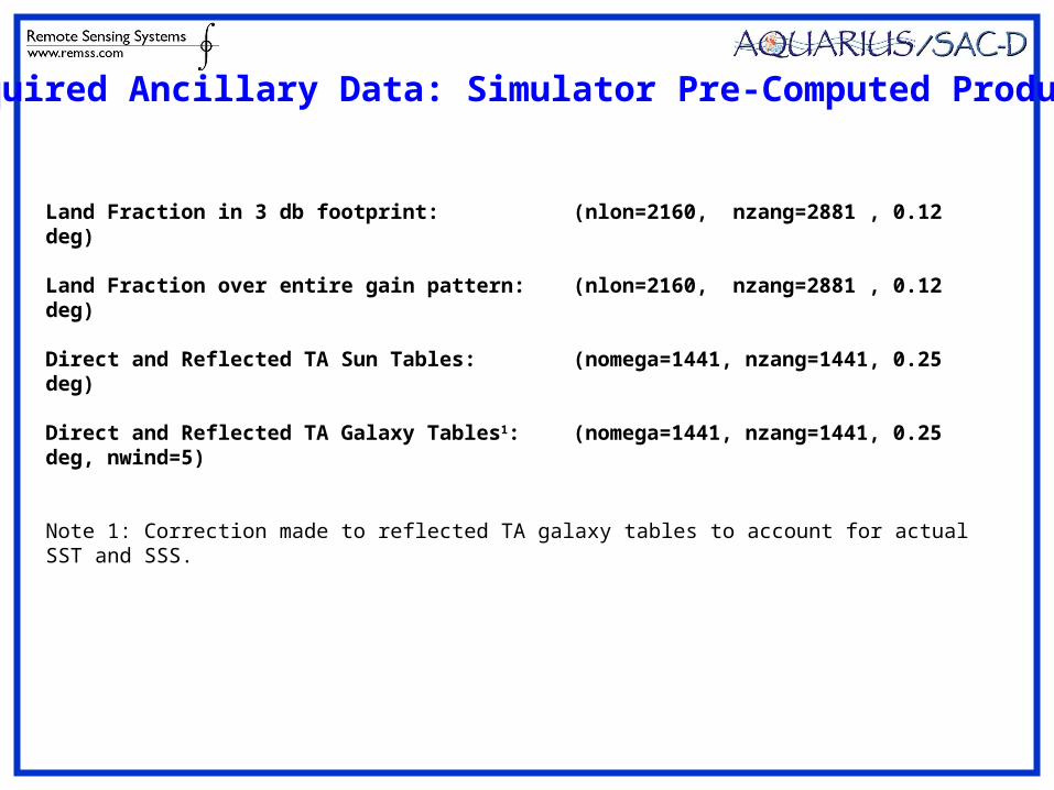
Land Fraction in 3 db footprint: (nlon=2160, nzang=2881 , 0.12 deg) Land Fraction over entire gain pattern: (nlon=2160, nzang=2881 , 0.12 deg)

Direct and Reflected TA Sun Tables: (nomega=1441, nzang=1441, 0.25 deg)

Direct and Reflected TA Galaxy Tables1: (nomega=1441, nzang=1441, 0.25 deg, nwind=5)

Note 1: Correction made to reflected TA galaxy tables to account for actual SST and SSS.

Required Ancillary Data: Simulator Pre-Computed Products

Julian Day

Orb

ital A

ngle

(Z

an

g)H-pol, Inner Horn

1 30 60 90 120 150 210 240 270 300 330 3650

60

120

180

240

300

360

0

0.02

0.04

0.06

Julian Day

Orb

ital A

ngle

(Z

an

g)

H-pol, Middle Horn

1 30 60 90 120 150 210 240 270 300 330 3650

60

120

180

240

300

360

0

0.02

0.04

0.06

Julian Day

Orb

ital A

ngle

(Z

an

g)

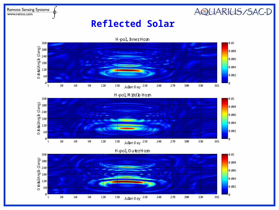
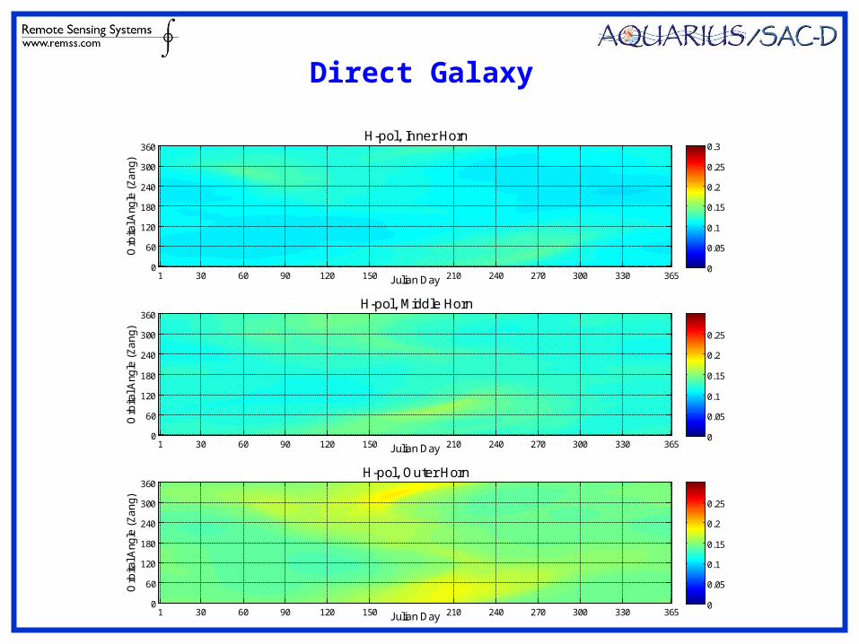
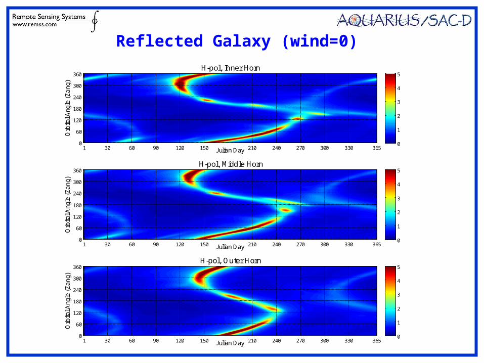
H-pol, Outer Horn

1 30 60 90 120 150 210 240 270 300 330 3650

60

120

180

240

300

360

0

0.02

0.04

0.06

Direct Solar

Julian Day

Orb

ital A

ngle

(Z

an

g)H-pol, Inner Horn

1 30 60 90 120 150 210 240 270 300 330 3650

60

120

180

240

300

360

0

0.002

0.004

0.006

0.008

0.01

Julian Day

Orb

ital A

ngle

(Z

an

g)

H-pol, Middle Horn

1 30 60 90 120 150 210 240 270 300 330 3650

60

120

180

240

300

360

0

0.002

0.004

0.006

0.008

0.01

Julian Day

Orb

ital A

ngle

(Z

an

g)

H-pol, Outer Horn

1 30 60 90 120 150 210 240 270 300 330 3650

60

120

180

240

300

360

0

0.002

0.004

0.006

0.008

0.01

Reflected Solar

Julian Day

Orb

ital A

ngle

(Z

an

g)H-pol, Inner Horn

1 30 60 90 120 150 210 240 270 300 330 3650

60

120

180

240

300

360

0

0.05

0.1

0.15

0.2

0.25

0.3

Julian Day

Orb

ital A

ngle

(Z

an

g)

H-pol, Middle Horn

1 30 60 90 120 150 210 240 270 300 330 3650

60

120

180

240

300

360

0

0.05

0.1

0.15

0.2

0.25

Julian Day

Orb

ital A

ngle

(Z

an

g)

H-pol, Outer Horn

1 30 60 90 120 150 210 240 270 300 330 3650

60

120

180

240

300

360

0

0.05

0.1

0.15

0.2

0.25

Direct Galaxy

Julian Day

Orb

ital A

ngle

(Z

an

g)H-pol, Inner Horn

1 30 60 90 120 150 210 240 270 300 330 3650

60

120

180

240

300

360

0

1

2

3

4

5

Julian Day

Orb

ital A

ngle

(Z

an

g)

H-pol, Middle Horn

1 30 60 90 120 150 210 240 270 300 330 3650

60

120

180

240

300

360

0

1

2

3

4

5

Julian Day

Orb

ital A

ngle

(Z

an

g)

H-pol, Outer Horn

1 30 60 90 120 150 210 240 270 300 330 3650

60

120

180

240

300

360

0

1

2

3

4

5

Reflected Galaxy (wind=0)

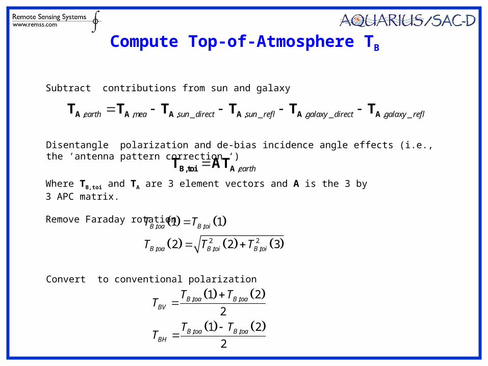
Where TB,toi and TA are 3 element vectors and A is the 3 by 3 APC matrix.

Remove Faraday rotation

,earthB,toi AT AT

, ,

2 2, , ,

1 1

2 2 3

B toa B toi

B toa B toi B toi

T T

T T T

, ,

, ,

1 2

21 2

2

B toa B toaBV

B toa B toaBH

T TT

T TT

, , , _ , _ , _ , _earth mea sun direct sun refl galaxy direct galaxy refl A A A A A AT T T T T T

Subtract contributions from sun and galaxy

Disentangle polarization and de-bias incidence angle effects (i.e., the ‘antenna pattern correction ‘)

Convert to conventional polarization

Compute Top-of-Atmosphere TB

, ,,

, , , _ , _,

, ,, _ , _,

,

,

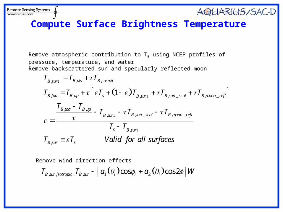
1

B dw B cosmicB sur

B toa B up s B sun scat B moon reflB sur

B toa B upB sun scat B moon reflB sur

s B sur

B sur s

T T T

T T T T T T

T TT T T

T T

T T Valid for all surfaces

, , , 1 2cos cos2B sur isotropic B sur i r iT T a a W

Remove atmospheric contribution to TB using NCEP profiles of pressure, temperature, and waterRemove backscattered sun and specularly reflected moon

Remove wind direction effects

Compute Surface Brightness Temperature

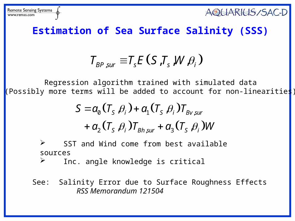
Estimation of Sea Surface Salinity (SSS)

, , , ,BP sur s s iT T E S T W

0 1 ,

2 , 3

, ,

, ,

S i S i Bv sur

S i Bh sur S i

S a T a T T

a T T a T W

Regression algorithm trained with simulated data(Possibly more terms will be added to account for non-linearities)

SST and Wind come from best available sources Inc. angle knowledge is critical

See: Salinity Error due to Surface Roughness Effects RSS Memorandum 121504

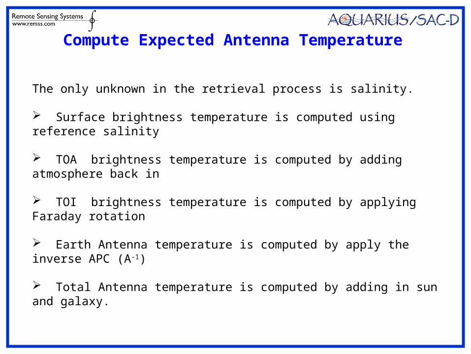
Compute Expected Antenna Temperature

The only unknown in the retrieval process is salinity.

Surface brightness temperature is computed using reference salinity

TOA brightness temperature is computed by adding atmosphere back in

TOI brightness temperature is computed by applying Faraday rotation

Earth Antenna temperature is computed by apply the inverse APC (A-1)

Total Antenna temperature is computed by adding in sun and galaxy.

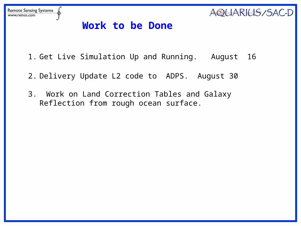
1. Get Live Simulation Up and Running. August 16

2. Delivery Update L2 code to ADPS. August 30

3. Work on Land Correction Tables and Galaxy Reflection from rough ocean surface.

Work to be Done

Backup Slide on Algorithm Performance

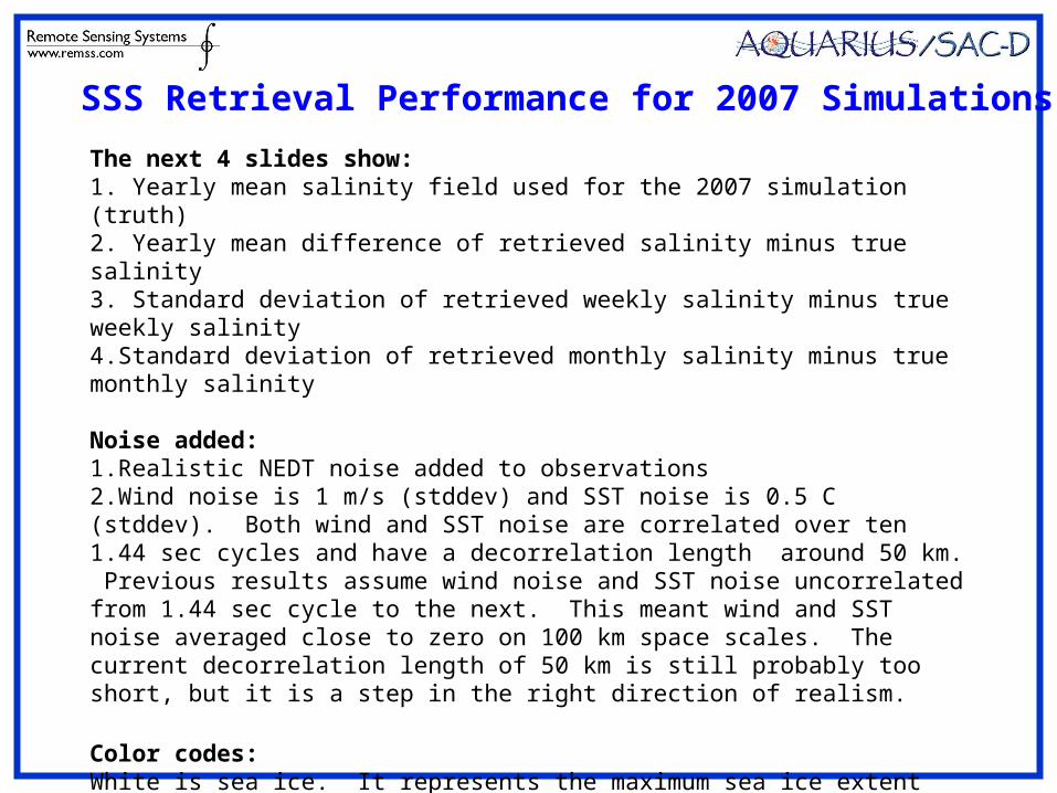
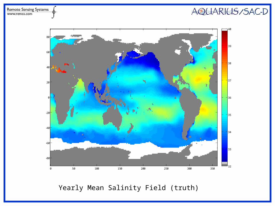
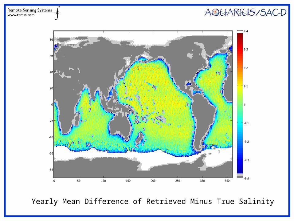
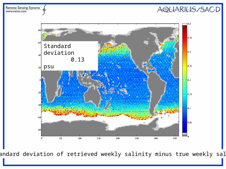
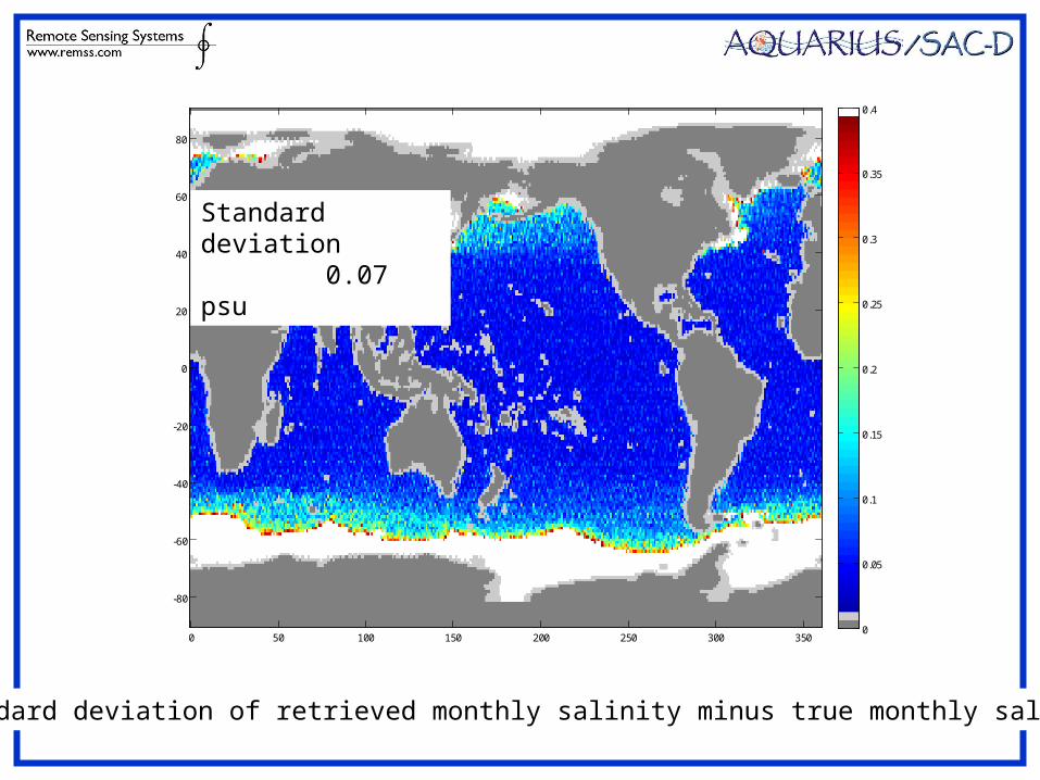
The next 4 slides show:1. Yearly mean salinity field used for the 2007 simulation (truth)2. Yearly mean difference of retrieved salinity minus true salinity3. Standard deviation of retrieved weekly salinity minus true weekly salinity4.Standard deviation of retrieved monthly salinity minus true monthly salinity

Noise added:1.Realistic NEDT noise added to observations2.Wind noise is 1 m/s (stddev) and SST noise is 0.5 C (stddev). Both wind and SST noise are correlated over ten 1.44 sec cycles and have a decorrelation length around 50 km. Previous results assume wind noise and SST noise uncorrelated from 1.44 sec cycle to the next. This meant wind and SST noise averaged close to zero on 100 km space scales. The current decorrelation length of 50 km is still probably too short, but it is a step in the right direction of realism.

Color codes:White is sea ice. It represents the maximum sea ice extentLight gray denotes land contamination exceeding 0.2%Dark gray denotes land contamination exceeding 5%.

SSS Retrieval Performance for 2007 Simulations

0 50 100 150 200 250 300 350

-80

-60

-40

-20

0

20

40

60

80

32

33

34

35

36

37

38

39

40

Yearly Mean Salinity Field (truth)

0 50 100 150 200 250 300 350

-80

-60

-40

-20

0

20

40

60

80

-0.4

-0.3

-0.2

-0.1

0

0.1

0.2

0.3

0.4

Yearly Mean Difference of Retrieved Minus True Salinity

0 50 100 150 200 250 300 350

-80

-60

-40

-20

0

20

40

60

80

0

0.05

0.1

0.15

0.2

0.25

0.3

0.35

0.4

Standard deviation of retrieved weekly salinity minus true weekly salinity

Standard deviation 0.13 psu

0 50 100 150 200 250 300 350

-80

-60

-40

-20

0

20

40

60

80

0

0.05

0.1

0.15

0.2

0.25

0.3

0.35

0.4

Standard deviation of retrieved monthly salinity minus true monthly salinity

Standard deviation 0.07 psu

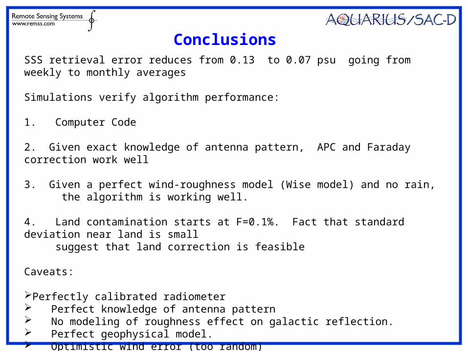
SSS retrieval error reduces from 0.13 to 0.07 psu going from weekly to monthly averages

Simulations verify algorithm performance:

1. Computer Code

2. Given exact knowledge of antenna pattern, APC and Faraday correction work well

3. Given a perfect wind-roughness model (Wise model) and no rain, the algorithm is working well.

4. Land contamination starts at F=0.1%. Fact that standard deviation near land is small suggest that land correction is feasible

Caveats:

Perfectly calibrated radiometer Perfect knowledge of antenna pattern No modeling of roughness effect on galactic reflection. Perfect geophysical model. Optimistic wind error (too random) Perfect modeling of rain

Conclusions