Mechanics and Mechanical EngineeringVol. 13, No. 2 (2009) 5–21c© Technical University of Lodz

Fracture of the Nonlinear Multi–Layered Composites

MieczysÃlaw Jaroniek

Technical University of ÃLodz,Department of Materials and Structures Strength

Stefanowskiego 1/15, 90-924 ÃLodz, Poland

Received (18 May 2009)Revised (25 May 2009)Accepted (20 Juli 2009)

Advanced mechanical and structural applications require accurate assessment of thedamage state of materials during the fabrications as well as during the service. Due tothe complex nature of the internal structure of the material, composites including thelayered composite often fail in a variety of modes.

Fabrication of the functionally graded materials (FGM) can be obtained by layeredmixing of two materials of different thermo–mechanical properties with different volumeratios gradually changed from layer to layer such that first layer has only a few particlesof the other phase and last has maximum volume ratio of this other phase. The material(FGM) is functionally graded thermal and stress barrier.

Between the ceramic layer and metallic bond layer there exist a functionally gradedlayer ”2” that contains volume of the bond (metallic) phase as a function of the distancey from he bond layer and volume ratio of the ceramics phase also as a function of ydistance from the bond layer.

The failure modes very often are influenced by the local material properties thatmay develop in time under heat and pressure, local defect distribution, process inducedresidual stress, and other factors.

Fracture problems in the layer can be studied using J integral in finite elementmethod, because it is not path independent

Consider a laminate composite in plane stress conditions, multi–layered beam bondedto planes. The fracture mechanics problem will be analysed using the photoelastic visu-alisation of the fracture events in a model structure

Keywords: Composites, multi–layered beams, fracture mechanic, photoelastic method,finite element method

1. Introduction

Fabrication of the model of the FGM can be obtained by layered mixing of twophotoelastic materials of different thermo-mechanical properties with different vol-ume ratios gradually changed from layer to layer such that first layer has only afew particles of the other phase and last has maximum volume ratio of this otherphase.

6 Jaroniek, M

The development of the failure criterion for a particular application is also veryimportant for the predictions of the crack path and critical loads.

Recently, there has been a successful attempt to formulate problems of multi-ple cracks without any limitation. This attempt was concluded with the series ofpapers summarising the undertaken research for isotropic [2], anisotropy [4] andnon–homogeneous class of problems [5] and [4].

Crack propagation in multi–layered composites of finite thickness is especiallychallenging and open field for investigation. Some results have been recently re-ported in [5]. The numerical calculations were carried out using the finite elementprograms ANSYS 9 and 10 [11]. Two different methods were used: solid modelingand direct generation.

2. Material properties

Material properties exert an influence on the stress distribution and concentration,damage process and load carrying capacity of elements. In the case of elastic–plastic materials, a region of plastic strains originates in most heavily loaded cross–sections. In order to visualise the state of strains and stresses, some tests have beenperformed on the samples made of an ”araldite”–type optically active epoxy resin(Ep–53), modified with softening agents in such a way that an elastic material hasbeen obtained. Properties of the components of experimental model are given inTab. 1.

Table 1 Mechanical properties of the experimental model components

Layer Young’sModulusEi [MPa]

Poisson’sratioνi [1]

Photoelasticconstants in termsof stresseskσ [MPa/fr]

Photoelasticconstants in termsof strainfε [-/fr]

1 3450.0 0.35 1.68 6.572 ·10−4

2 1705.0 0.36 1.18 9.412 ·10−4

3 821.0 0.38 0.855 14.31 ·10−4

4 683.0 0.40 0.819 16.79 ·10−4

3. Experimental Results

The stress distribution in was determined using two methods:Shear Stress Difference Procedure (SDP – evaluation a complete stress

state by means the isochromatics and the angles of the isoclines along the cuts) [3].Method of the characteristics (the stress distribution were determined using

the isochromatics only and the equations of equilibrium [10].In a general case [7], the Cartesian components of stress: σx , σy and τxy in the

neighbourhood of the crack tip are:

σx = KI√2πr

cos Θ2 (1− sin Θ

2 sin 3Θ2 ) + σox

σy = KI√2πr

cos Θ2 (1 + sin Θ

2 sin 3Θ2 ) (1)

τxy = 1√2πr

[KI sin Θ2 cos Θ

2 cos 3Θ2 ) + KII cos Θ

2 (1− sin Θ2 sin 2Θ

2 )]

Fracture of the Nonlinear ... 7

From which:

(σ1 − σ2)2 =1

2πr

[(KI sinΘ + 2KII cosΘ)2 + (KII sinΘ)2

]

(2)

−2σox√2πr

sinΘ2

[KI sinΘ(1 + 2 cos Θ) + KII(1 + 2 cos2 Θ + cos Θ)

]+ σ2

ox

where KI and KII are the stress–intensity factors, r and θ are coordinates of apolar coordinate system.

By inserting the values kσmi = σ1 − σ2 into (2) we obtain the isochromaticscurves in polar coordinates (r, Θ). For each isochromatic loop the position ofmaximum angle Θm corresponds to the maximum radius of the rm. This principlecan also be used in the mixed mode analysis [7] by employing information from twoloops in the near field of the crack, if the far field stress component – σox(Θ) = const.Differentiating Eqn (2) with respect to Θ, setting Θ = Θm and r = rm and usingequation ∂τm/∂Θm = 0 gives:

g(KI ,KII , σox) =1

2πr

[K2

I sin 2Θ + 4KIKII cos 2Θ− 3K2II sin 2Θ

]

−2σox√2πrr

sinΘ2{ [KI(cos Θ + 2 cos 2Θ)−KII(2 sin 2Θ + sin Θ)]

+12

cosΘ2

[Ki(sinΘ + sin 2Θ) + KII(2 + cos 2Θ + cos Θ)] } (3)

f(KI ,KII , σox) = (σ1 − σ2)2 − (kσm)2 = 0

g(KI ,KII , σox) =∂[(σ1 − σ2)2]

∂Θm= 0

Substituting the radii rm and the angles Θm from these two loops into a pair ofequations of the form given in Eqn (3) gives two independent relations dependenton the parameters KI , KII and σox. The third equation is obtained by using (2).The three equations obtained in this way have the form

gi(KI ,KII , σox) = 0gj(KI ,KII , σox) = 0 (4)fk(KI ,KII , σox) = 0

In order to determine KI , KII and σox it is sufficient to select two arbitrary pointsri, Θi and apply the Newton–Raphson method to the solution of three simultaneousnon–linear equations (4).

The values KC according to mixed mode of the fracture were obtained from

KC =√

K2I + K2

II (5)

Example of the numerical results obtained from (4):m = 12.5, r1 = 0.6 mm, Θ1 = 1.484, r2 = 10.45 mm, Θ2 = 1.416,K

(4)I = 0.14 MPa

√m, K

(4)II = 1.05 MPa

√m, σox = 0.039 MPa,

K(4)C = 1.05 MPa

√m

8 Jaroniek, M

a)

y

x

a

P

l = 210 mm

P

cracks

Strain gauges

1

2

3

4

E j=E(x)

1

2

3

4

100 mm

10

10

9.0

11

10

b)

c)

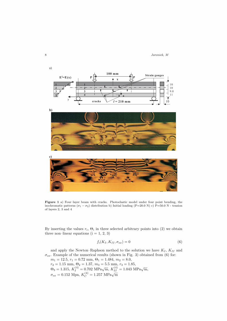
Figure 1 a) Four–layer beam with cracks. Photoelastic model under four point bending, theisochromatic patterns (σ1 − σ2) distribution b) Initial loading (P=20.0 N) c) P=50.0 N - tensionof layers 2, 3 and 4

By inserting the values ri, Θi in three selected arbitrary points into (2) we obtainthree non–linear equations (i = 1, 2, 3)

fi(KI ,KII , σox) = 0 (6)

and apply the Newton–Raphson method to the solution we have KI , KII andσox. Example of the numerical results (shown in Fig. 3) obtained from (6) for:

m1 = 12.5, r1 = 0.72 mm, Θ1 = 1.484, m2 = 8.0,r2 = 1.15 mm, Θ2 = 1.37, m3 = 5.5 mm, r3 = 1.85,Θ3 = 1.315, K

(4)I = 0.702 MPa

√m, K

(4)II = 1.043 MPa

√m,

σox = 0.152 Mpa, K(4)C = 1.257 MPa

√m

Fracture of the Nonlinear ... 9

A B

A B

Figure 2 The isochromatic patterns (σ1 − σ2) distribution according to the propagation of thecrack obtained experimentally

P=540N-15.41MPa

m=4.55

3.72MPa

5.5 MPa

2.95MPam=2.95

5.77MPa

m=4.1

sx

3.98MPa

m=6.25

Mg=27000Nm

m

A

A

m=3.5

-3.54MPa

-5.88 MPa

e=4.5mm

P=540N-17.64MPa

2.78 MPa

2.57 „

5.51 MPa

2.95 MPa

41.1 MPa

sx

5.45 MPa

Mg=29700Nmm

BS

BS

-3.45MPa

-4.29 MPa

0.5 mm

Figure 3 Distribution of stresses in cros sections A-A and B-B 0.5mm with respect to crackobtained experimentally

4. The stress analysis from complex potentials

In the present paper the elastic and plastic deformation has been approximatelyanalysed using the Muskhelishvili’s complex potentials method.

σxx + σyy = 4Re [ψ′ (z)]σyy − σxx + 2iτxy = 2 [zψ′′ (z) + χ′′ (z)]2G (u + iυ) = κψ (z)− zψ′ (z)− χ′ (z)2G (u′ + iυ′) = κψ′ (z)− zψ′ (z)− zψ”(z)− χ” (z)

10 Jaroniek, M

where κ = 3− 4ν for plain strain and κ = 3−ν1+ν plain stress

σxx + σyy = 4Re [ψ′ (z)]σyy − σxx = Re2 [zψ′′ (z) + χ′′ (z)]τxy = Im [zψ′′ (z) + χ′′ (z)]

The elastostatic stress field is required to satisfy the well–known equilibrium equa-tions [1] using two analytic functions ψ(z) and χ(z)

σxx = Re [2ψ′ (z)− zψ′′ (z)− χ′′ (z)]σyy = Re [2ψ′ (z) + zψ′′ (z) + χ′′ (z)]τxy = Im [zψ′′ (z) + χ′′ (z)] (7)2G (u + iυ) = κψ (z)− zψ′ (z)− χ′ (z)χ′′(z) = −zψ′′ (z)

Using two analytic functions ψ(z) and χ(z)

ψ′ (z) = ψ′1 (z) + ψ′2 (z) χ′′(z) = z [ψ′′1 (z)− ψ′′2 (z)]

The complex stress potentials are assumed as follows

2ψj(z) =N∑

n=1

[Cn

∫z(2−n)

√z − a

z + adz

]

2ψ′(j) (z) =N∑

n=1

√z − a

z + aCj

nz(2−n)

2ψ2(z) =N∑

n=1

[Dn

∫z(3−n)dz√

z2 − a2

](8)

2ψ′2(z) =N∑

n=1

[Dnz(3−n)

√z2 − a2

]

The stress σx , σy and τxy characterizes by

σx = Re [2ψ′ − 2xψ′′1 ]− yIm2ψ′′2σy = Re [2ψ′ + 2xψ′′1 ] + yIm2ψ′′2τxy = xIm2ψ′′1 − yRe2ψ′′2

The stress–intensity factors are related by:

KI = limx→a

σy (x, 0)√

2π (x− a)

KII = limx→a

τxy (x, 0)√

2π (x− a)

GC = 2a∫0

p (x)uy (x, 0) dx

KI = limx→a

σy (x, 0)√

2π (x− a)

KII = limx→a

τxy (x, 0)√

2π (x− a)

GC = 2a∫0

p (x)uy (x, 0) dx

(9)

Fracture of the Nonlinear ... 11

1

2

M

3

x

y

a

ey

sy

sysy=txy=0

M

x0

xj

xj –x0

x1

Figure 4 The boundary conditions for 3 layer beam and isochromatic patterns (σ1 − σ2) distri-bution corresponding to vertical crack

By inserting the (8) into (9) we obtain

K(j)I = lim

x→a

{Re

[2ψ′(j) (z)

]+ x2ψ′′(j) (z)

} √2π (x− a)

K(j)II = lim

x→a

{xIm

[2ψ”(j) (z)

]}√2π (x− a)

and

σjx =

N∑n=1

{Re

[(C

j

n + iCj

n)f1(z) + (Dj

n + iDj

n)f2(z)]}

−N∑

n=1

{yIm

[(D

j

n + iDj

n)f3(z)]}

σjy =

N∑n=1

{Re

[(C

j

n + iCj

n)f4(z) + (Dj

n + iDj

n)f2(z)]}

(10)

+N∑

n=1

{yIm

[(D

j

n + iDj

n)f3(z)]}

τ jxy =

N∑n=1

{xIm

[(C

j

n + iCj

n)f5(z)]}

−N∑

n=1

{yRe

[(D

j

n + iDj

n)f3(z)]}

For y = 0 in this case, the Cartesian components of stress: σx, σy and τxy are givenas:

12 Jaroniek, M

σjx =

N∑n=1

{Re

[(C

j

n + iCj

n)f1(z)]}

σjy =

N∑n=1

{Re

[(C

j

n + iCj

n)f4(z)]}

(11)

τ jxy =

N∑n=1

{xIm

[(C

j

n + iCj

n)f5(z)]}

f1(z) =1

zn−1

(1z

√z − a

z + a− x

az − (n− 2)(z2 − a2)(z + a)

√z2 − a2

)

f2(z) =z3−n

√z2 − a2

f3(z) = z2−n (3− n)(z2 − a2) + z2

(z2 − a2)3/2

f4(z) =1

zn−1

(1z

√z − a

z + a+ x

az − (n− 2)(z2 − a2)(z + a)

√z2 − a2

)

f5(z) =1

zn−1

az(n− 2)(z2 − a2)(z + a)

√z2 − a2

Cin = ReCi

n + iImCin

Din = ReDi

n + iImDin

Cin = ReCi

n

Cin = ImCi

n

(12)

The boundary conditions can by expressed as

σ(∞)y − σ(∞)

x + 2iτ (∞)xy = (z − z) 2ψ” (z) + 2A

σg = −M

I(x− s) = σ∞y σ∞x = 0 (13)

εjy = εj+1

y εjy = ∂υj

∂y εjx = εj+1

x

u′ =∂u

∂xuj = uj+1 υj = υj+1

Fracture of the Nonlinear ... 13

20 19.1 18.2 17.3 16.4 15.5 14.6 13.7 12.8 11.9 1122

23.2

24.4

25.6

26.8

28

29.2

30.4

31.6

32.8

3432.1

22.1

xi

11.53-19.982- s yi

12 10.2 8.4 6.6 4.8 3 1.2 0.6 2.4 4.2 610

11.2

12.4

13.6

14.8

16

17.2

18.4

19.6

20.8

2220.6

10.35

xi

4.40710.675- s yi

0 9 18 27 36 45 54 63 72 81 908

8.3

8.6

8.9

9.2

9.5

9.8

10.1

10.4

10.7

11

xi

syi

1

2

3

x

ya

s2y

s1y = –19.9 MPa

s3y = 81.5 MPa

s y = txy = 0

M Msy(max) = 81.5 MPa

sy= 4.5 MPa

sy = 4.2 MPa

sy = –11.8 MPa

sy = –11.5 MPa

sy = –19.88 MPa

Figure 5 Distribution of stresses in cross sections A-A and B-B 0.5mm with respect to crackobtained experimentally and used in the analysis of the complex potentials

H∫

0

σjydx

=N∑

n=1

Re

H∫

0

[Cj

n

zn−1

(1z

√z − a

z + a+ x

az − (n− 2)(z2 − a2)(z + a)

√z2 − a2

)]dx

= 0

H∫

0

bσjyxdx + M (14)

=N∑

n=1

H∫

0

bRe[

Cjn

zn−1

(1z

√z − a

z + a+ x

az − (n− 2)(z2 − a2)(z + a)

√z2 − a2

)]dx

+ M = 0

σjy =

N∑n=1

{Re

[Cj

n

zn−1

(1z

√z − a

z + a+ x

az − (n− 2)(z2 − a2)(z + a)

√z2 − a2

)]}

σg = −M

I(x− s) = σ∞y

For each isochromatic loop σ1 − σ2 = kσm

σyy − σxx = kσmt cos 2α (15)

14 Jaroniek, M

in other hand σ1 + σ2 = σxx + σyy and

σxx + σyy =N∑

n=1

2Re[Cnz(2−n)

√z − a

z + a+

Dnz(3−n)

√z2 − a2

](16)

This principle can be used in the analysis of the stresses, by inserting the valuesmi, αi in selected arbitrary points P (ri, Θi) we obtain equations

N∑n=1

{Re

[(Cn + iCn)[f4(z)− f1(z)]

]+ 2yIm

[(Dn + iDn)f3(z)

]}= kσmi cos 2αi

from which:

K(j)II = lim

x→a

N∑n=1

{xIm

[Cj

nf4(z)] √

2π(x− a)}

(17)

K(j)II = lim

x→a

N∑n=1

{xIm

[Cj

nf5(z)] √

2π(x− a)}

τ2m = Re [zψ′′ (z) + χ′′ (z)]2 + Im [zψ′′ (z) + χ′′ (z)]2 (18)

τ2m =

(N∑

n=1

{xRe [Cnf5(z)] + yIm [Dnf3(z)]})2

+

(N∑

n=1

{xIm [Cnf5(z)]− yRe [Dnf3(z)]})2

For each isochromatic loop

εyy − εxx =1

2G′

N∑n=1

{Re

[(Cn + iCn)[f4(z)− f1(z)]

]+ 2yIm

[(Dn + iDn)f3(z)

]}

in other hand εyy − εxx = fε(m)m cos 2α and

(1 + νj)Ej

N∑n=1

{Re

[(C

j

n + iCj

n)[f4(z)− f1(z)]]

+ 2yIm[(D

j

n + iDj

n)f3(z)]}

= fεm(xt) cos 2α

KI = limx→a

N∑n=1

{Re

[Cn

zn−1

(1z

√z − a

z + a+ x

az − (n− 2)(z2 − a2)(z + a)

√z2 − a2

)

+Dnz3−n

√z2 − a2

] √2π(x− a)

}(19)

KII = limx→a

N∑n=1

{xIm

[Cn

zn−1

az(n− 2)(z2 − a2)(z + a)

√z2 − a2

] √2π(x− a)

}

Fracture of the Nonlinear ... 15

8 7 6 5 4 3 2 1 0 1 2 3 4 5 6 7 8

2

1.4

0.8

0.2

0.4

1

1.6

2.2

2.8

3.4

4

trace 1

trace 2

trace 3

trace 4

2.963

1.57-

x1i

x2i

x3i

x4i

7.6517.651- y1 i y2 i, y3 i, y4 i,

0.9mm

7.5 mm9.0 mm

-7.8 mm

x

y

a)

b)

1.5 mm

4

5

4.5

m = 4.0

s1- s2 = 6.72

m = 5.5

s1- s2 = 9.24

m = 7.0

s1- s2 = 11.8

m = 9.0

s1- s2 = 15.12

m = 4.0

m = 5.5

x

1 mm

y

M = 7

6

3

7

Figure 6 The isochromatic patterns (σ1 − σ2) distribution according to the propagation of thecrack obtained experimentally and used in the analysis of the complex potentials

Where

zl

√z − a

z + a= rl

(r1

r2

)1/2 [cos

(Θ1 + Θ2

2+ Θl

)+ i sin

(Θ1 + Θ2

2+ Θl

)]

zl

√z2 − a2

=rl

(r1r2)1/2

[cos

(Θl − Θ1 + Θ2

2

)+ i sin

(Θl − Θ1 + Θ2

2

)]

Photoelastic measurements make possible deformations and stresses study in wholestructure of elastomer. On basis of photoelastic measurements, we define directlydifference of strains:

σ1 − σ2 = kδm

ε1 − ε2 =1 + ν

E(σ1 − σ2) =

1 + ν

Ekδm (20)

16 Jaroniek, M

where:fσ =

1 + ν

Ekδ

fε =1 + ν

Ekσ

model constants corresponding to difference of stresses and main deformations.As well as it is known lines for which differences between stresses and main

strains have constant value and one color are called isochromatics. Next, basingon isochromatics measurements stresses distribution has been defined. Applyingstress–strain relation, in elastic body deviator strain components are proportionalto deviator stress component, as written:

σ1 − σsr

ε1 − εsr=

σ2 − σsr

ε2 − εsr(21)

Photoelastic measurements results one can apply also for strain and stress analyseconcerning elasto–plastic materials. In elasto–plastic body, proportion of deviatorstrain components and deviator stress components is described by relation:

σ1 − σsr

ε1 − εsr=

σ2 − σsr

ε2 − εsr= 2G′ (22)

where

G′ =τ0

γ0

(τ

γ0

)N−1

Es

1 + νs=

2σo

εpoεp−1

3− (1− 2νo)(

εεo

)p−1

σ1 − σ2 =2σo

εpoεp−1

3− (1− 2νo)(

εεo

)p−1 (ε1 − ε2)

σ1 − σ2

ε1 − ε2=

2σo

εpoεp−1

3− (1− 2νo)(

εεo

)p−1

For simply tensile test, when σ1 = σ, σ2= σ3= 0, parameters ε1 = εint , ε2 andε3 one can determine on the basis of shape change low ε2 = ε3 = − 1

2 (εint − 3εsr),

where σint = σ = AεP and εint =(

1Aσint

)1/p or σsr = σ/3.Main strains difference amount:

ε1 − ε2 = 32εint − 3εsr (23)

ε1 − ε2 =32α0εpl

(J

α0σplεplIn

) n1+n

r−n

n+1 σn−1int

[(σrr − σθθ)

2 − (2τrθ)2]1/2

(24)

Where σ2int = σ2

rr + σ2θθ − σrrσθθ + 3σ2

rθ

σ1 − σ2 = σpl

(J

α0σplεplIn

) 11+n

r−1

n+1

[(σrr − σθθ)

2 − (2τrθ)2]1/2

(25)

Fracture of the Nonlinear ... 17

On basis of photoelastic measurements, we define directly difference of strains:

σ1 − σ2 = kδm

ε1 − ε2 =1 + ν

E(σ1 − σ2) =

1 + ν

Ekδm

By inserting the values ε1 − ε2 into (24) we obtain the isochromatics curves inpolar coordinates (r, Θ).

rε (Θ) =(

32

α0εpl

fεm

)n+1n

(J

α0σplεplIn

)σ

n2−1n

int

[(σrr − σθθ)

2 − (2τrθ)2]n+1

2n

(26)

In elasto–plastic body, proportion of deviator strain components and deviator stresscomponents is described by:

σ1 − σ2

ε1 − ε2=

σpl32αεpl

(J

α0σplεplIn

) 1−n1+n

r−1−nn+1 σ1−n

int (27)

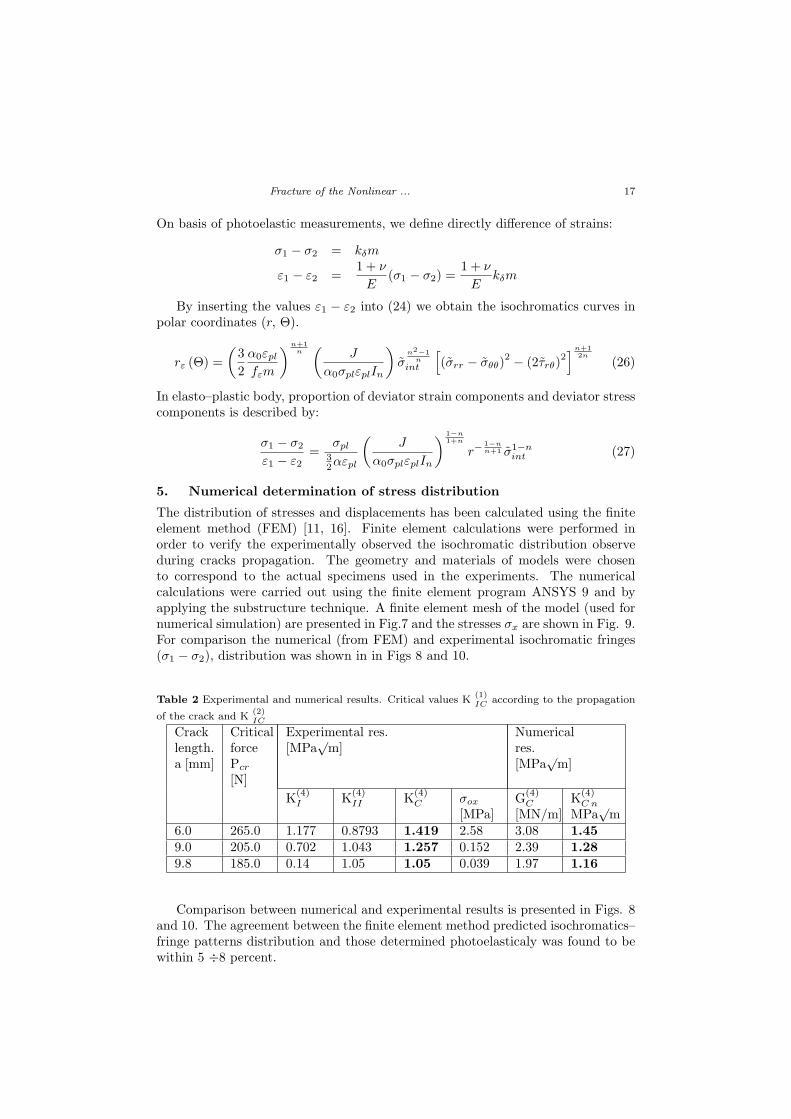
5. Numerical determination of stress distribution

The distribution of stresses and displacements has been calculated using the finiteelement method (FEM) [11, 16]. Finite element calculations were performed inorder to verify the experimentally observed the isochromatic distribution observeduring cracks propagation. The geometry and materials of models were chosento correspond to the actual specimens used in the experiments. The numericalcalculations were carried out using the finite element program ANSYS 9 and byapplying the substructure technique. A finite element mesh of the model (used fornumerical simulation) are presented in Fig.7 and the stresses σx are shown in Fig. 9.For comparison the numerical (from FEM) and experimental isochromatic fringes(σ1 − σ2), distribution was shown in in Figs 8 and 10.

Table 2 Experimental and numerical results. Critical values K(1)IC according to the propagation

of the crack and K(2)IC

Cracklength.a [mm]

CriticalforcePcr

[N]

Experimental res.[MPa

√m]

Numericalres.[MPa

√m]

K(4)I K(4)

II K(4)C σox

[MPa]G(4)

C

[MN/m]K(4)

C n

MPa√

m6.0 265.0 1.177 0.8793 1.419 2.58 3.08 1.459.0 205.0 0.702 1.043 1.257 0.152 2.39 1.289.8 185.0 0.14 1.05 1.05 0.039 1.97 1.16

Comparison between numerical and experimental results is presented in Figs. 8and 10. The agreement between the finite element method predicted isochromatics–fringe patterns distribution and those determined photoelasticaly was found to bewithin 5 ÷8 percent.

18 Jaroniek, M

h1

h2

h3

h4

1

2

3

4

y1

y3

y2

y5y4

a

Figure 7 A finite element mesh of the model (for numerical simulation)

Figure 8 Numerical determination of stress distribution (Ansys 5.6). Distribution of the stressesσx (cracks length a=6.0 mm )

Fracture of the Nonlinear ... 19

sy

y

x sc= –18.58B

B

smax = 52.56

1 – Layer

2 – Layer

3 – Layer

4 – Layer

Crack

Figure 9 Numerical determination of stress distribution (Ansys 9). Distribution of the normalstress σx and equivalent stress σint along the crack

Figure 10 Experimental determination of stress distribution (The stress intensity). Distributionof the absolute values of σ1 − σ2 (cracks length a=6.0 mm )

20 Jaroniek, M

6. Conclusions

Fabrication of the model of the FGM can be obtained similarly as the function-ally graded materials by layered mixing of two photoelastic materials of differentthermo–mechanical properties with different volume ratios gradually changed fromlayer to layer such that first layer has only a few particles of the other phase andlast has maximum volume ratio of this other phase. Photoelasticity was shown tobe promising in stress analysis of beams with various numbers and orientation ofcracks.

In the present paper the elastic deformation has been approximately analysedusing the Muskhelishvili’s complex potentials method in the analysis of the stresses.Using two analytic functions in the analysis of the stresses we obtain equations forisochromatic loop.

The specimen can be build as layered beam, for example,glass layer at the bottom then particles of the same glass in the epoxy in several

layers of various volume ratio of the glass in epoxy and pure epoxy at the top.The beam can be loaded in bending to generate cracks while will propagate

through the FGM layer.It is possible to fabricate a model using various photoelastic materials to model

multi layered structure.Finite element calculations (FEM) were performed in order to verify the ex-

perimentally observed branching phenomenon and the isochromatic distributionobserved during cracks propagation. The agreement between the finite elementmethod predicted isochromatics–fringe patterns distribution and those determinedphotoelasticaly was found to be within 3÷5 percent.

References

[1] Cherepanov G.P.: Mechanics of brittle fracture, Mc Graw – Hill, New York, 1979.

[2] Cook T.S. and Erdogan F.: Stresses in bonded materials with a crack perpendic-ular to the interface, Int. Journ. of Engineering Science, Vol. 10, 677–697, 1972.

[3] Frocht M.M.: Photoelasticity, John Wiley, New York, 1960.

[4] Gupta A.G.: Layered composite with a broken laminate, International Journal ofSolids and Structures, No36 (1845-1864), 1973.

[5] Hilton P.D. and Sin G.C.: A laminate composite with a crack normal to interfaces,International Journal of Solids and Structures, No 7, 913, 1971.

[6] Rychlewska J. and Wozniak C.: Boundary layer phenomena in elastodynamics offunctionally graded laminates, Archives of Mechanics, 58, 4–5, 431–444, 2006.

[7] Sanford R.J. and Dally J.: A General Method For Determining Mixed–Mode StressIntensity Factors From Isochromatic Fringe Patterns, —textitEng. Fract. Mech., Vol.2, 621–633, 1979.

[8] Szczepinski W.: A photoelastic method for determining stresses by meansisochromes only, Arch. of Applied Mechanics, 5 (13), Warsaw, 1961.

[9] Szymczyk J. and Wozniak C.: Continuum modelling of laminates with a slowlygraded microstructure, Archives of Mechanics, 58, 4-5, 445–458, 2006.

[10] Theocaris P.S. and Gdoutos E.E.: A photoelastic determination of KI stressintensity factors, Eng. Fract. Mech., Vol. 7, 331–339, 1975.

[11] User’s Guide ANSYS : Ansys 9, Inc., Huston, USA, 2006.

Fracture of the Nonlinear ... 21

[12] Wozniak C.: Nonlinear Macro–Elastodynamics of Microperiodic Composites, Bull.Ac. Pol. Sci.: Tech. Sci., 41, 315–321, 1993.

[13] Wozniak C.: Microdynamics: Continuum. Modelling the Simple Composite Materi-als, J. Theor. Appl. Mech., 33, 267–289, 1995.

[14] Wozniak C.: Nonlinear Macro–Elastodynamics of Microperiodic Composites, Bull.Ac. Pol. Sei.: Tech. Sei., 41, 315–321, 1993.

[15] Wozniak C.: Microdynamics: Continuum. Modelling the Simple Composite Materi-als, J. Theor. Appl. Mech., 33, 267–289, 1995.

[16] Zienkiewicz O.C.: The Finite Element Method in Engineering Science, Mc Graw –Hill, London, New York, 1971.