Fractional-order uniaxial visco-elasto-plastic models … · Fractional-order uniaxial...

Available online at www.sciencedirect.com

ScienceDirect

Comput. Methods Appl. Mech. Engrg. 308 (2016) 443–467www.elsevier.com/locate/cma

Fractional-order uniaxial visco-elasto-plastic models for structuralanalysis

J.L. Suzukia,d, M. Zayernourib,c, M.L. Bittencourta, G.E. Karniadakisd,∗

a Department of Integrated Systems, Faculty School of Mechanical Engineering, University of Campinas, SP 13083-970, Brazilb Department of Computational Mathematics, Science, and Engineering (CMSE), Michigan State University, MI 48824, USA

c Department of Mechanical Engineering, Michigan State University, MI 48824, USAd Division of Applied Mathematics, Brown University, Providence, RI 02912, USA

Received 12 January 2016; received in revised form 23 May 2016; accepted 25 May 2016Available online 1 June 2016

Highlights

• Two fractional-order visco-elasto-plastic models are developed, namely M1 and M2.• Model M1 uses a rate-dependent yield function via time-fractional Caputo derivative.• Model M2 uses a visco-plastic regularization via time-fractional Caputo derivative.• A fractional return-mapping algorithm is developed for each model.• Results show flexibility of the fractional-orders and recovery of classical models.

Abstract

We propose two fractional-order models for uniaxial large strains and visco-elasto-plastic behavior of materials in structuralanalysis. Fractional modeling seamlessly interpolates between the standard elasto-plastic and visco-elasto-plastic models, takinginto account the history (memory) effects of the accumulated plastic strain to specify the state of stress. To this end, we developtwo models, namely M1 and M2, corresponding to visco-elasto-plasticity considering a rate-dependent yield function and visco-plastic regularization, respectively. Specifically, we employ a fractional-order constitutive law that relates the Kirchhoff stress tothe Caputo time-fractional derivative of the strain with order β ∈ (0, 1). When β → 0 the standard rate-independent elasto-plastic model with linear isotropic hardening is recovered by the models for general loading, and when β → 1, the correspondingclassical visco-plastic model of Duvaut–Lions (Perzyna) type is recovered by the model M2 for monotonic loading. Since thematerial behavior is path-dependent, the evolution of the plastic strain is achieved by fractional-order time integration of the plasticstrain rate with respect to time. The plastic strain rate is then obtained by means of the corresponding plastic slip and properconsistency conditions. Finally, we develop the so called fractional return-mapping algorithm for solving the nonlinear system ofthe equilibrium equations developed for each model. This algorithm seamlessly generalizes the standard return-mapping algorithmto its fractional counterpart. We test both models for convergence subject to prescribed strain rates, and subsequently we implementthe models in a finite element truss code and solve for a two-dimensional snap-through instability problem. The simulation resultsdemonstrate the flexibility of fractional-order modeling using the Caputo derivative to account for rate-dependent hardening and

∗ Corresponding author.E-mail address: [email protected] (G.E. Karniadakis).

http://dx.doi.org/10.1016/j.cma.2016.05.0300045-7825/ c⃝ 2016 Elsevier B.V. All rights reserved.

http://crossmark.crossref.org/dialog/?doi=10.1016/j.cma.2016.05.030&domain=pdf

http://www.elsevier.com/locate/cma

http://dx.doi.org/10.1016/j.cma.2016.05.030

http://www.elsevier.com/locate/cma

mailto:[email protected]

http://dx.doi.org/10.1016/j.cma.2016.05.030

444 J.L. Suzuki et al. / Comput. Methods Appl. Mech. Engrg. 308 (2016) 443–467

viscous dissipation, and its potential to effectively describe complex constitutive laws of engineering materials and especiallybiological tissues.c⃝ 2016 Elsevier B.V. All rights reserved.

Keywords: Fractional-order constitutive laws; History-dependent visco-elasto-plasticity; Large strains; Time-fractional integration

1. Introduction

Fractional differential operators appear in many systems in science and engineering such as visco-elastic materials[1–3], electrochemical processes [4] and porous or fractured media [5]. For instance, it has been found that the trans-port dynamics in complex and/or disordered systems is governed by non-exponential relaxation patterns [6,7]. Forsuch processes, a time-fractional equation, in which the time-derivative emerges as Dν

t u(t), appears in the continuouslimit. One interesting application of fractional calculus is to model complex elasto-plastic behavior of engineeringmaterials (e.g. [8,9]). Recently, fractional calculus has been employed as an effective tool for modeling materials ac-counting for heterogeneity/multi-scale effects to the constitutive model [10–12], where the fractional visco-plasticitywas introduced as a generalization of classical visco-plasticity of Perzyna type [13]. The fundamental role of theformulation is the definition of the flow rule by introducing a fractional gradient of the yield function. Also, a con-stitutive model for rate-independent plasticity based on a fractional continuum mechanics framework accounting fornonlocality in space was developed in [14].

Formulating fast and accurate numerical methods for solving the resulting system of fractional ODEs/PDEsin such problems is the key to incorporating such nonlocal/history-dependent models in engineering applications.Efficient discretization of the fractional operators is crucial. Lubich [15,16] pioneered the idea of discretized fractionalcalculus within the spirit of finite-difference method (FDM). Later, Sanz-Serna [17] adopted the idea of Lubich andpresented a temporal semi-discrete algorithm for partial integro-differential equations, which was first order accurate.Sugimoto [18] also employed a FDM for approximating the fractional derivative emerging in Burgers’ equation.Later on, Gorenflo et al. [19] adopted a finite-difference scheme by which they could generate discrete models ofrandom walk in such anomalous diffusion. Diethelm et al. proposed a predictor–corrector scheme in addition to afractional Adams method [20,21]. After that, Langlands and Henry [22] considered the fractional diffusion equation,and analyzed the L1 scheme for the time-fractional derivative. Sun and Wu [23] also constructed a difference schemewith L∞ approximation of the time-fractional derivative. Of particular interest, Lin and Xu [24] analyzed a FDM forthe discretization of the time-fractional diffusion equation with order (2 − α). However, there are other classes ofglobal methods (spectral and spectral element methods) for discretizing fractional ODEs/PDEs (e.g., [25–28]), whichare efficient for low-to-high dimensional problems. Furthermore, Zayernouri and Matzavinos developed a fractionalfamily of schemes, called fractional Adams–Bashforth and fractional Adams–Moulton method for high-order explicitand implicit treatment of nonlinear problems [29]. There were recent developments on meshless approaches appliedto fractional-diffusion and space-fractional advection–dispersion problems [30,31]. Also, Chen [32] developed a newdefinition of fractional Laplacian and applied to three-dimensional, nonlocal heat conduction.

The main contribution of the present work is to propose and solve two fractional-order models, namely M1 andM2, for uniaxial large strains and visco-elasto-plastic behavior of materials. Both models account for fractionalvisco-elastic modeling by defining a stress–strain relationship involving the Caputo time derivative of fractional-order, but have distinct formulations to model the fractional visco-plasticity. For the model M1, visco-plasticity isachieved by including history effects in time for the internal hardening parameter in the yield function, making it rate-dependent. Differently from some works found in the literature [10–12], we do not modify the flow rule. The modelM2 accounts for a rate-independent yield function without an internal hardening parameter, and the visco-plasticeffect is achieved based on the approach of visco-plastic regularization used in the classical visco-plastic model ofDuvaut–Lions type (which is equivalent to Perzyna’s model). Furthermore, the models consider different memoryeffects for visco-elasticity and visco-plasticity. Both models are used within the framework of a time-fractionalbackward-Euler integration procedure with a fractional return-mapping algorithm, based on the classical modelsin the literature [9,8]. The developed algorithm seamlessly generalizes the standard return-mapping algorithm to itsfractional counterpart, making it amenable for path-dependent visco-elasto-plastic analyses in engineering and bio-

J.L. Suzuki et al. / Comput. Methods Appl. Mech. Engrg. 308 (2016) 443–467 445

engineering applications. We also present the standard nonlinear finite element formulation for trusses and show thatthe only required modifications are in the stress update procedure, which will be described in constitutive boxes foreach model.

Several numerical analyses are performed to investigate the behavior of the models. We test the algorithmspresented in terms of convergence using a benchmark solution, then we perform tests with cyclic strains to accountfor hysteresis behavior. Both models are implemented in the context of finite element method (FEM) using an updatedLagrangian approach to solve a two-bar snap-through problem. Because no analytical solutions are derived, weimplemented the classical one-dimensional models for elasto-plasticity with linear hardening and visco-plasticityof Duvaut–Lions type, and we recover these limit cases for verification. We verify that both fractional-ordermodels recover the classical rate-independent elasto-plastic model for general loading/unloading conditions, and alsointerpolate between plastic/visco-plastic behavior with the variation of the fractional-order parameters. The obtainedresults show the flexibility of the fractional-order models to describe the rate-dependent hardening and viscousdissipation. This motivates the application of the models developed in this work to identify material parameters ofcomplex constitutive laws of engineering materials and biological tissues.

2. Definitions of fractional calculus

We start with some preliminary definitions of fractional calculus [33]. The left-sided Riemann–Liouville integralsof order µ, when 0 < µ < 1, are defined, as

(RLxL

I µx f )(x) =

1Γ (µ)

x

xL

f (s)

(x − s)1−µds, x > xL , (1)

where Γ represents the Euler gamma function and xL denotes the lower integration limit. The corresponding inverseoperator, i.e., the left-sided fractional derivatives of order µ, is then defined based on Eq. (1) as

(RLxL

Dµx f )(x) =

d

dx(RL

xLI 1−µ

x f )(x) =1

Γ (1 − µ)

d

dx

x

xL

f (s)

(x − s)µds, x > xL . (2)

Furthermore, the corresponding left-sided Caputo derivatives of order µ ∈ (0, 1) are obtained as

(CxL

Dµx f )(x) =

RLxL

I 1−µx

d f

dx

(x) =

1Γ (1 − µ)

x

xL

f ′(s)

(x − s)µds, x > xL . (3)

The definitions of Riemann–Liouville and Caputo derivatives are linked by the following relationship, which can bederived by a direct calculation

(RLxL

Dµx f )(x) =

f (xL)

Γ (1 − µ)(x + xL)µ+ (C

xLDµ

x f )(x), (4)

which denotes that the definitions of the aforementioned derivatives coincide when dealing with homogeneousDirichlet initial/boundary conditions.

3. Kinematics of large visco-elasto-plastic deformations

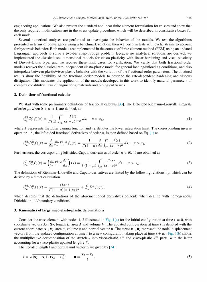
Consider the truss element with nodes 1, 2 illustrated in Fig. 1(a) for the initial configuration at time t = 0, withcoordinate vectors X1, X2, length L , area A and volume V . The updated configuration at time t is denoted with thecurrent coordinates x1, x2, area a, volume v and normal vector n. The terms u1, u2 represent the nodal displacementvectors from the updated configuration at time t to a new configuration taking place at time t + dt . Fig. 1(b) showsthe multiplicative decomposition of the stretch λ into visco-elastic λve and visco-plastic λvp parts, with the latteraccounting for a visco-plastic updated length lvp.

The updated length l and normal unit vector n are given by [34]

l =

(x2 − x1) · (x2 − x1), n =

x2 − x1

l, (5)


(a) Truss element in 2D space. (b) Stretch decomposition.

Fig. 1. (a) Kinematics of the truss in terms of initial and updated configurations; (b) Multiplicative decomposition of the stretch into visco-elasticand visco-plastic parts, taking place from the initial to the updated configuration.

where the updated coordinates of the element nodes are denoted as

x1 =

x1y1

, x2 =

x2y2

. (6)

We consider the decomposition of the stretch illustrated in Fig. 1(b) for the truss element when subject to a changein configuration. The visco-elastic and visco-plastic stretches are given by

λve=

l

lvp , λvp=

lvp

L. (7)

The total stretch is given by

λ = λveλvp=

l

L. (8)

Applying the natural logarithm to the above equation, we obtain an additive decomposition given by [8]

ln(λ) = ln(λve) + ln(λvp), (9)

which is called logarithmic strain and is usually denoted as

ε = εve+ εvp. (10)

The logarithmic strain measure defined in Eq. (9) is thermodynamically conjugate to the Kirchhoff stress τ [8], whichwill be addressed in the next section, along with the constitutive equations for the visco-elasto-plastic models.

4. Fractional-order visco-elasto-plastic models

We consider two visco-elasto-plastic models, called M1 and M2. The developed framework for both modelsincorporates memory effects for the evaluation of visco-elasto-plastic large strains. We present the mathematicalformulation for each model and an efficient algorithm to solve the nonlinear system of fractional-order differentialequations, and remark on how the models recover the classical local models.

To account for the memory effects in time, we modify the classical models presented in the literature [8,9]. Themodel M1 is a modification of classical elasto-plasticity with linear hardening and the model M2 is a modification ofvisco-plasticity of Duvaut–Lions type. For this purpose, we introduce Scott–Blair elements with fractional-order β,which interpolate between linear spring when β → 0 and viscous Newton element when β → 1 [1].

The memory effects for both models will be presented in the stress–strain relationship regarding the visco-elasticpart, which is evaluated for the entire time domain. To account for memory effects in visco-plasticity, we willconsider the Caputo time-fractional derivative in the yield function for the model M1, while for the model M2 we willincorporate the memory effects via a separate equation that describes the visco-plastic regularization. The memoryfor the fractional derivatives describing visco-plasticity will be considered starting from the last attained yield stress.


(a) Diagram with rheological elements. (b) Stress versus strain response.

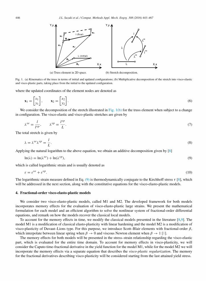
Fig. 2. Visco-elasto-plastic model M1. (a) Constitutive diagram with the rheological elements for visco-elasticity and visco-plasticity. (b) Stressversus strain response described by the yield function (Eq. (16)), showing the expansion of the visco-elastic boundary from ∂ Eτ (point A) to ∂ E∗

τ

(point B) after exceeding the yield stress.

4.1. Model M1

The model M1 is illustrated in Fig. 2(a), consisting of a Scott–Blair element with constant E [Pa · sβE ] and afractional-order βE for the visco-elastic part with corresponding visco-elastic strain εve. The visco-plastic deviceconsists of a parallel combination of a Coulomb frictional element with yield stress τY

[Pa], a linear hardening springwith constant H [Pa], a Scott–Blair element with constant K [Pa · sβK ] and fractional-order βK . The correspondingvisco-plastic strain is denoted by εvp. The term τ [Pa] stands for the Kirchhoff stress.

We start by rewriting Eq. (10) in terms of the visco-elastic strain component:

εve= ε − εvp. (11)

The history-dependent constitutive law for this model is assumed to be of the form:

τ = E C0 DβE

t (εve) = E C0 DβE

t (ε − εvp), 0 < βE < 1. (12)

To satisfy the homogeneous initial conditions for the Caputo time derivative, we assume the given point of thematerial to have no initial strains, that is, ε(t = 0) = εve(t = 0) = εvp(t = 0) = 0. In this sense, we observe that theRiemann–Liouville definition (Eq. (2)) could also be employed, since we consider homogeneous initial conditions.To designate a set of admissible stresses, we define the following closed convex stress space:

Eτ = τ ∈ R | f (τ, α) ≤ 0, (13)

where f : R × R+→ R represents the yield condition, defined by

f (τ, α) := |τ | −τ y′

+ Hα, (14)

where

τ y′= τ y

+ K Ctp

DβKt (α), 0 < βK < 1, (15)

with α representing an internal hardening variable with initial condition α(t = 0) = 0, that is, we assume no initialhardening. The term τ y denotes an yield stress which is updated according to unloading conditions (τ y

= τY in thebeginning of the process) and tp denotes the time of onset of plasticity. The term τ y′ in Eq. (15) can be interpretedas an updated yield stress accounting for memory effects in visco-plasticity, while the term Hα represents a localhardening parameter.

The time tp for plasticity is reset when we unload the material from a visco-plastic state, and the yield stress isupdated to a new value τ y′. Substituting Eq. (15) into Eq. (14), we obtain

f (τ, α) := |τ | −

τ y

+ K Ctp

DβKt (α) + Hα

. (16)

We do not consider different time derivative limits for Eq. (12) because plastic strains inevitably take place in thevisco-elastic range. Notice that we included the Caputo derivative of order βK inside f (τ, α), thus making the yield


(a) Diagram with rheological elements. (b) Stress versus strain response.

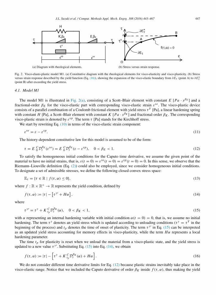
Fig. 3. Visco-elasto-plastic model M2 considering visco-plastic regularization. (a) Constitutive diagram with the rheological elements for visco-elasticity and visco-plasticity. (b) Stress versus strain response: path A–B described by the yield function (Eq. (20)), which is visco-elastic perfectlyplastic; path A–B’ with the stress response after the visco-plastic regularization (V-P-R) procedure (Eq. (22)). The relaxation path B’–B occurs atconstant strain levels and t → ∞ (compared to the relaxation time of the material).

condition rate-dependent. The corresponding boundary of Eτ is the convex set denoted by ∂Eτ , given as

∂Eτ = τ ∈ R | f (τ, α) = 0, (17)

where f (τ, α) = 0 is the so-called consistency condition in the classical elasto-plastic models. In the present model,we assume that the hardening is isotropic in the sense that at any state of loading the center of Eτ remains at theorigin of the stress–strain domain. The expected stress versus strain response based on Eqs. (16) and (17) is presentedin Fig. 2(b). The consistency condition (Eq. (17)) will be addressed in incremental form in time to derive the visco-plastic solutions. Moreover, similar to classical elasto-plasticity, the evolution of hardening is assumed to be linear interms of the visco-plastic strain rate. Therefore

α = |εvp|, (18)

and the flow rule is not modified, and is given by

εvp= γ sign(τ ), (19)

where γ denotes the amount of plastic slip, also with initial condition γ (t = 0) = 0, and the term sign(τ ) representsthe direction of the plastic flow. Recalling Eq. (16) and the definition of the fractional derivative, when βK → 0,we recover the limit case without rate effects (spring) and the constant K accounts for the standard plastic modulusof rate-independent plasticity, with units of [Pa]. On the other hand, if βK → 1 we recover the limit case of a localinteger-order derivative (dashpot), where K would be equivalent to the material viscosity η, with corresponding unitsof [Pa · s].

4.2. Model M2

The schematic diagram of the model M2 is illustrated in Fig. 3(a), which consists of the same elements as themodel M1, except that we remove the linear hardening spring with constant H in the visco-plastic part.

The stress–strain relation for this model is the same as Eq. (12). We consider the yield function of perfect plasticitygiven by

f (τ ) := |τ | − τ y′, (20)

where we consider the yield stress τ y′= τY when t = 0 and update it when the material is unloaded from visco-

plastic behavior (more details will be addressed in Section 6). Because the model is based on visco-plasticity ofDuvaut–Lions type, we use the idea of visco-plastic regularization in [9] to take into account the memory effect of thevisco-plastic strain εvp when we obtain an over-stressed level f (τ ) > 0:

K Ctp

DβKt (εvp) = τ − τ∞, (21)

where τ∞ is the relaxed stress when t → ∞ (compared to the natural relaxation time of the material). Substitutingthe stress–strain relation from Eq. (12) into Eq. (21), and rearranging the visco-plastic strains to the left-hand-side, weobtain

E C0 DβE

t (εvp) + K Ctp

DβKt (εvp) = E C

0 DβEt (ε) − τ∞. (22)


The solution for this model involves determination of the rate-independent stress τ∞ by applying the consistencycondition to Eq. (20) and substituting the result into Eq. (22) to determine the visco-plastic strains εvp. After that, thetime-dependent stress can be determined from the constitutive relation (Eq. (12)). Fig. 3(b) presents the stress versusstrain response in the relaxed state (path O-A-B) described by the yield function (Eq. (20)) and the regularized state(path O-A-B’) achieved with Eq. (22). More details about this procedure will be presented after the time discretizationscheme. We note that when βK → 1 in Eq. (22) we recover the local first-order derivatives and therefore the classicalDuvaut–Lions formulation.

4.2.1. Remark about parameter HWe note that when we set the linear hardening parameter H = 0 in the model M1, we obtain the same diagram

for both models. However, the approaches are still different, since the model M1 considers the Caputo-time fractionalderivative in the yield function (Eq. (16)) while the model M2 uses an yield function of visco-elastic perfectly plasticbehavior and accounts for visco-plastic regularization with relaxation effects described by Eq. (21).

4.2.2. Remark about visco-elastic/plastic memory effectsThe initial study of the presented models considered the entire time domain for the visco-plastic equations (16),

(22) without updating the yield stress τ y . However, for model M1 it was observed that due to long memory effectsand no update in the yield stress, the visco-elastic range did not expand in an isotropic way when cyclic loads wereapplied. Furthermore, for the model M2, we obtained non-physical results for the visco-plastic part without updatingthe yield stress τ y′ due to lack of internal hardening combined with long memory on visco-plastic strains.

We consider the distinction between “visco-elastic time” and “visco-plastic time” a more natural way of treatingthe memory effects, since in a general problem the material will not be in a visco-plastic state (Eqs. (17) and (22)) atall times. On the other hand, the stress–strain relation (Eq. (12)) is used regardless of the stress state.

5. Time integration and discretization in space

For notation purposes, we denote variables at times tn, tn+1 by the lower-scripts n, n+1, respectively. The governingequations on the equilibrium of a truss are discretized in time and space to obtain (e.g., see [35])

ψn+1 = Mb1 (un+1 − un) − b2vn − b3an

+ Rn+1 − Pn+1 = 0, (23)

where we denote ψn+1 as the residual force vector, M as the global mass matrix for all nodes, Rn+1 as theglobal internal force vector dependent of the updated configuration with coordinates xn+1, which in turn dependon the displacements un+1. The term Pn+1 represents the global external nodal force vector. The terms an and vn ,respectively, denote the global acceleration and velocity vectors. More details regarding the Newmark scheme arepresented in Appendix B with the description of the approximation coefficients bi . We do not consider a lineardamping matrix in Eq. (23) because the constitutive law will naturally introduce damping effects for both visco-elastic/plastic contributions.

We note that our approach can be employed in the context of any standard numerical method e.g., finite elementmethod (FEM), spectral element methods, etc. This is particularly true because our history-dependent modeling resultsin a system of time-fractional equations. Hence, the spatial domain can be always treated using available standarddiscretizations. However, the computation of the incremental stresses needs special care as shown in the sequel.

The equilibrium system (Eq. (23)) is linearized by employing Newton’s method using incremental globaldisplacements, defined as

uk+1n+1 = uk

n+1 + ∆u. (24)

Accordingly, the updated global coordinates are given by

xk+1n+1 = xn + uk+1

n+1, (25)

where the superscript k + 1 refers to the current iteration of the Newton’s method. The linearized form of Eq. (23) inthe direction of a displacement increment ∆u is given by the following system of equations:

b1M + KkTn+1

∆u = −M

b1(uk

n+1 − un) − b2vn − b3an

− Rk

n+1 + Pn+1. (26)


The terms un , vn , an are obtained from the last converged time step n. The term KT is the tangent stiffness matrix andis updated at each iteration k along with the internal force vector. In the linear finite element spatial discretization, theelement tangent stiffness for the current formulation is given by (see [8])

K(e)T =

K11 K12K21 K22

, with K11 =

KC

l3

(x2 − x1)

2 (x2 − x1)(y2 − y1)

(x2 − x1)(y2 − y1) (y2 − y1)2

+

aσ

l

1 00 1

, (27)

where the superscript (e) denotes the local elemental operation associated with the eth element, and K22 = K11, K12 =

K21 = −K11. The term l denotes the current element length, x1, x2, y1, y2 denote the element updated coordinates,σ denotes the Cauchy stress at the element, and KC is given by

KC = aV

v

∂τ

∂ε− 2aσ. (28)

The relation between the Kirchhoff and Cauchy stresses is given by τ =vV σ . We note that there is no assumption

in the constitutive behavior, therefore the formulation presented in this section is general. The local stress derivativein terms of strain in Eq. (28) is known as tangent modulus, and its computation will be addressed in the next section.Notice that this derivative is local in nature, and comes from the linearized kinematics of the problem. The elementalinternal force vector and the corresponding mass matrix are given by

R(e)=

aσ

l

x2 − x1y2 − y1x1 − x2y1 − y2

, M(e)=

ρ AL

6

2 0 1 00 2 0 11 0 2 00 1 0 2

, (29)

where ρ is the material density. In the next section we determine the current stress τn+1 and tangent modulus

∂τ∂ε

n+1

for the fractional-order models.

6. Fractional return-mapping algorithms

We present the time-fractional backward-Euler integration procedure for both fractional models, where a trial stateis defined by freezing the internal variables and a fractional return-mapping algorithm is obtained enforcing the properconditions. For the model M1, the solution for the plastic slip is given by a fractional-order differential equation. Forthe model M2 we solve a fractional-order differential equation for the visco-plastic strain instead, using the idea ofvisco-plastic regularization.

The backward-Euler procedure is implicit in time, unconditionally stable and is first-order accurate. We assume thatat time tn+1, with t ∈ [0, T ] all variables for the previous time step tn are known. We consider a strain increment ∆εn ,which in the context of the standard finite element method, can be obtained using Eqs. (8) and (9) from an increase inelement length ∆l, calculated from the displacement increments ∆u (Eq. (26)). From the constitutive model point ofview, we just consider this increment to be known, regardless of being prescribed or obtained by the equilibrium ofthe system. The strain for time tn+1 is given by

εn+1 = εn + ∆εn . (30)

The stress–strain relation is given by

τn+1 = E C0 DβE

tε − εvp

t=tn+1. (31)

The incremental flow rule and evolution of the hardening parameter are, respectively, given by

εvpn+1 = ε

vpn + ∆γ sign (τn+1) , (32)

αn+1 = αn + ∆γ, (33)

where ∆γ denotes the plastic slip for the time interval [tn, tn+1] under consideration. In our fractional return-mappingalgorithm, we make use of the so called trial state, where we freeze the internal variables of the model at time tn+1 in


the following way:

εvptr ial

n+1 = εvpn , αtr ial

n+1 = αn . (34)

Having the trial visco-plastic strain defined, we perform a trial visco-elastic stress given by

τ tr ialn+1 = E C

0 DβEt

ε − εvptr ial

t=tn+1

, (35)

where we will keep the term εvptr ialinstead of ε

vpn for notation purposes, since the time-fractional Caputo derivative

is evaluated at time tn+1. The trial state defined in Eq. (34) will be substituted in the discrete form of the fractionalCaputo derivatives, which is presented in Section 6.1. The result of Eq. (35) is applied in a trial yield function f tr ial

n+1in order to check if the stress state lies within the visco-elastic or over the visco-plastic ranges, and perform thereturn-mapping procedure if necessary.

The current visco-plastic reference time is denoted here as tpn+1 , and is updated when a new yield stress is achievedfrom cyclic behavior. We introduce an auxiliary notation to track this visco-plastic time by using an incrementalvariable pn+1. The initial value is considered to be p0 = 0. In the incremental procedure, we account for the currenttime step pn+1 = 0 if the state is visco-elastic. The value pn+1 = n + 1 is set when the stress state exceeds the yieldstress, coming from a visco-elastic state. When the stress state is an increasing visco-plastic state (without change ofload direction), the visco-plastic time reference is the same as the previous step, that is, pn+1 = pn .

6.1. Algorithm for the model M1

The yield function (Eq. (16)) at time tn+1 is given by

fn+1 = |τn+1| −

τ y

+ Hαn+1 + K Ctpn+1

DβKt (α)

t=tn+1

. (36)

Considering the definition of the trial state, we obtain

f tr ialn+1 = |τ tr ial

n+1 | −

τ y

+ Hαn + K Ctpn

DβKt

αtr ial

t=tn+1

, (37)

where the Caputo time-fractional derivative of αtr ial is taken starting from time tpn , because it is the availableinformation about the last known yield stress τ y . If f tr ial

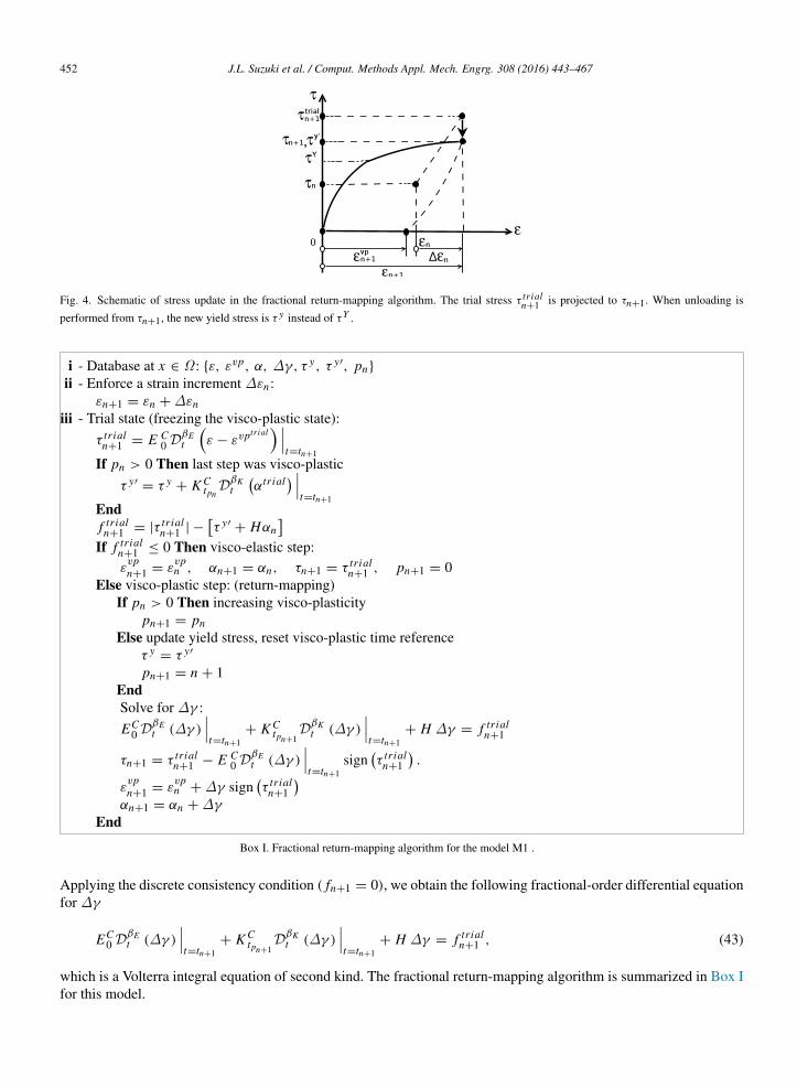
n+1 ≤ 0 we are within the visco-elastic range. Otherwise,we have an inadmissible stress indicating the onset of visco-plasticity. We enforce the discrete consistency conditionfn+1 = 0 to obtain the solution for ∆γ and then to perform a projection of the trial stress onto the yield surface, asillustrated in Fig. 4. Substituting Eq. (32) into Eq. (31), and recalling Eq. (35), we obtain

τn+1 = τ tr ialn+1 − E C

0 DβEt (∆γ )

t=tn+1

sign (τn+1) . (38)

We can rewrite the above equation as

|τn+1| sign(τn+1) = |τ tr ialn+1 | sign(τ tr ial

n+1 ) − E C0 DβE

t (∆γ )

t=tn+1

sign (τn+1) , (39)

hence,|τn+1| + EC

0 DβEt (∆γ )

t=tn+1

sign(τn+1) = |τ tr ial

n+1 | sign(τ tr ialn+1 ). (40)

The terms inside the brackets must be positive since ∆γ > 0 and E > 0, and therefore

sign(τn+1) = sign(τ tr ialn+1 ). (41)

Substituting Eqs. (38) and (33) into Eq. (36) and recalling Eqs. (37) and (41), yields

fn+1 = f tr ialn+1 − H∆γ − EC

0 DβEt (∆γ )

t=tn+1

− K Ctpn+1

DβKt (∆γ )

t=tn+1

. (42)


Fig. 4. Schematic of stress update in the fractional return-mapping algorithm. The trial stress τ tr ialn+1 is projected to τn+1. When unloading is

performed from τn+1, the new yield stress is τ y instead of τY .

i - Database at x ∈ Ω : ε, εvp, α, ∆γ, τ y, τ y′, pn

ii - Enforce a strain increment ∆εn :εn+1 = εn + ∆εn

iii - Trial state (freezing the visco-plastic state):

τ tr ialn+1 = E C

0 DβEt

ε − εvptr ial

t=tn+1

If pn > 0 Then last step was visco-plastic

τ y′= τ y

+ K Ctpn

DβKt

αtr ial

t=tn+1

Endf tr ialn+1 = |τ tr ial

n+1 | −τ y′

+ Hαn

If f tr ialn+1 ≤ 0 Then visco-elastic step:εvpn+1 = ε

vpn , αn+1 = αn, τn+1 = τ tr ial

n+1 , pn+1 = 0Else visco-plastic step: (return-mapping)

If pn > 0 Then increasing visco-plasticitypn+1 = pn

Else update yield stress, reset visco-plastic time referenceτ y

= τ y′

pn+1 = n + 1EndSolve for ∆γ :

EC0 DβE

t (∆γ )

t=tn+1

+ K Ctpn+1

DβKt (∆γ )

t=tn+1

+ H ∆γ = f tr ialn+1

τn+1 = τ tr ialn+1 − E C

0 DβEt (∆γ )

t=tn+1

signτ tr ial

n+1

.

εvpn+1 = ε

vpn + ∆γ sign

τ tr ial

n+1

αn+1 = αn + ∆γ

End

Box I. Fractional return-mapping algorithm for the model M1 .

Applying the discrete consistency condition ( fn+1 = 0), we obtain the following fractional-order differential equationfor ∆γ

EC0 DβE

t (∆γ )

t=tn+1

+ K Ctpn+1

DβKt (∆γ )

t=tn+1

+ H ∆γ = f tr ialn+1 , (43)

which is a Volterra integral equation of second kind. The fractional return-mapping algorithm is summarized in Box Ifor this model.


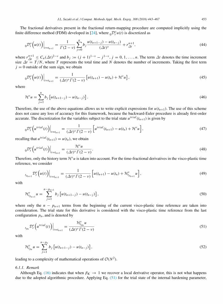
The fractional derivatives present in the fractional return-mapping procedure are computed implicitly using thefinite difference method (FDM) developed in [24], where 0 Dν

t u(t) is discretized as

0 Dνt

u(t)

t=tn+1

=1

Γ (2 − ν)

nj=0

b ju(tn+1− j ) − u(tn− j )

(∆t)ν+ rn+1

∆t , (44)

where rn+1∆t ≤ Cu(∆t)2−ν and b j := ( j + 1)1−ν

− j1−ν, j = 0, 1, . . . , n. The term ∆t denotes the time incrementsize ∆t = T/N , where T represents the total time and N denotes the number of increments. Taking the first termj = 0 outside of the sum sign, we obtain

0 Dνt

u(t)

t=tn+1

=1

(∆t)νΓ (2 − ν)

u(tn+1) − u(tn) + Hνu

, (45)

where

Hνu =

nj=1

b ju(tn+1− j ) − u(tn− j )

. (46)

Therefore, the use of the above equations allows us to write explicit expressions for u(tn+1). The use of this schemedoes not cause any loss of accuracy for this framework, because the backward-Euler procedure is already first-orderaccurate. The discretization for the variables subject to the trial state utr ial(tn+1) is given by

0 Dνt

utr ial(t)

t=tn+1

=1

(∆t)νΓ (2 − ν)

utr ial(tn+1) − u(tn) + Hνu

, (47)

recalling that utr ial(tn+1) = u(tn), we obtain

0 Dνt

utr ial(t)

t=tn+1

=Hνu

(∆t)νΓ (2 − ν). (48)

Therefore, only the history term Hνu is taken into account. For the time-fractional derivatives in the visco-plastic timereference, we consider

tpn+1Dν

t

u(t)

t=tn+1

=1

(∆t)νΓ (2 − ν)

u(tn+1) − u(tn) + Hν

tpn+1u, (49)

with

Hνtpn+1

u =

n−pn+1j=1

b ju(tn+1− j ) − u(tn− j )

, (50)

where only the n − pn+1 terms from the beginning of the current visco-plastic time reference are taken intoconsideration. The trial state for this derivative is considered with the visco-plastic time reference from the lastconfiguration pn , and is denoted by

tpnDν

t

utr ial(t)

t=tn+1

=

Hνtpn

u

(∆t)νΓ (2 − ν)(51)

with

Hνtpn

u =

n−pnj=1

b ju(tn+1− j ) − u(tn− j )

, (52)

leading to a complexity of mathematical operations of O(N 2).

6.1.1. RemarkAlthough Eq. (16) indicates that when βK → 1 we recover a local derivative operator, this is not what happens

due to the adopted algorithmic procedure. Applying Eq. (51) for the trial state of the internal hardening parameter,


we obtain

tpnDβK

t

αtr ial

t=tn+1

=HβK

tpnα

(∆t)βK Γ (2 − βK ). (53)

Recalling Eq. (50), when the fractional-order ν → 1, the associated weights b j → 0, and therefore the above equationfor the fractional derivative of αn vanish. This asymptotic case, in fact, leads to the following trial yield function:


n+1 | −τ y

+ Hαn. (54)

Therefore, the only remaining hardening effect relies on the rate-independent linear hardening term Hαn . If wecombine both effects βK → 1 and H = 0, we obtain a limit case of asymptotic perfect visco-plasticity, whichwill be observed in results of Section 7.2.

The above discussion shows that due to the employment of a trial state, there is no reason in using a local first orderderivative of the hardening parameter α in the definition of f (τ, α), since the term would vanish regardless of thematerial parameters. However, the inclusion of a fractional derivative introduces memory effects that do not vanish,except when βK → 1.

6.2. Algorithm for the model M2

We consider the same stress–strain relationship as the model M1, given by Eq. (31). The incremental yield functionis given by

fn+1 = |τn+1| − τ y′, (55)

with the corresponding trial function


n+1 | − τ y′. (56)

Substituting Eq. (31) into Eq. (55), and recalling Eqs. (32) and (56), we obtain

fn+1 = f tr ialn+1 − EC

0 DβEt (∆γ )

t=tn+1

. (57)

With the discrete consistency condition ( fn+1 = 0), we obtain the following fractional-order differential equation:

EC0 DβE

t (∆γ )

t=tn+1

= f tr ialn+1 . (58)

To calculate the rate-independent solution for stress, we use Eq. (38) replacing τn+1 with τ∞:

τ∞ = τ tr ialn+1 − EC

0 DβEt (∆γ )

t=tn+1

signτ tr ial

n+1

. (59)

Comparing Eqs. (58) and (59), we can rewrite Eq. (59) as

τ∞ = τ tr ialn+1 − sign(τ tr ial

n+1 ) f tr ialn+1 = sign(τ tr ial

n+1 ) τ y′. (60)

Therefore, the expression for τ∞ is given in a closed form. The algorithm to be used is of same type as the modelM1, but we consider an additional equation when solving for the visco-plastic step, which is the incremental form ofEq. (22), given by

EC0 DβE

tεvp

t=tn+1+ K C

tpn+1DβK

tεvp

t=tn+1= EC

0 DβEt (ε)

t=tn+1

− sign(τ tr ialn+1 ) τ y′. (61)

Also, we use an auxiliary incremental loading function denoted by f ∗

n+1 to check for unloading conditions in thevisco-plastic range, in order to perform an update in the yield stress in case of unloading:

f ∗

n+1 = |τ tr ialn+1 | − τn, (62)


i - Database at x ∈ Ω : ε, εvp, τ y, τ y′, τn, pn

ii - Enforce a strain increment ∆εn :εn+1 = εn + ∆εn

iii - Trial state (freezing the visco-plastic state):

τ tr ialn+1 = E C

0 DβEt

ε − εvptr ial

t=tn+1


n+1 | − τ y′

If f tr ialn+1 ≤ 0 Then visco-elastic step:εvpn+1 = ε

vpn , τn+1 = τ tr ial

n+1 pn+1 = 0Else visco-plastic step: (return-mapping)

If pn > 0 Then increasing visco-plasticitypn+1 = pn

Else reset visco-plastic time referencepn+1 = n + 1

Endf ∗

n+1 = |τ tr ialn+1 | − τn

If f ∗ < 0 Then unloading during visco-plastic step, update:τ y′

= |τn|

EndPerform visco-plastic regularization. Solve for ε

vpn+1:

EC0 DβE

t (εvp)

t=tn+1

+ K Ctpn+1

DβKt (εvp)

t=tn+1

= EC0 DβE

t (ε)

t=tn+1

− sign(τ tr ialn+1 ) τ y′

τn+1 = E C0 DβE

t (ε − εvp)

t=tn+1

.

End

Box II. Fractional return-mapping algorithm with visco-plastic regularization for the model M2 .

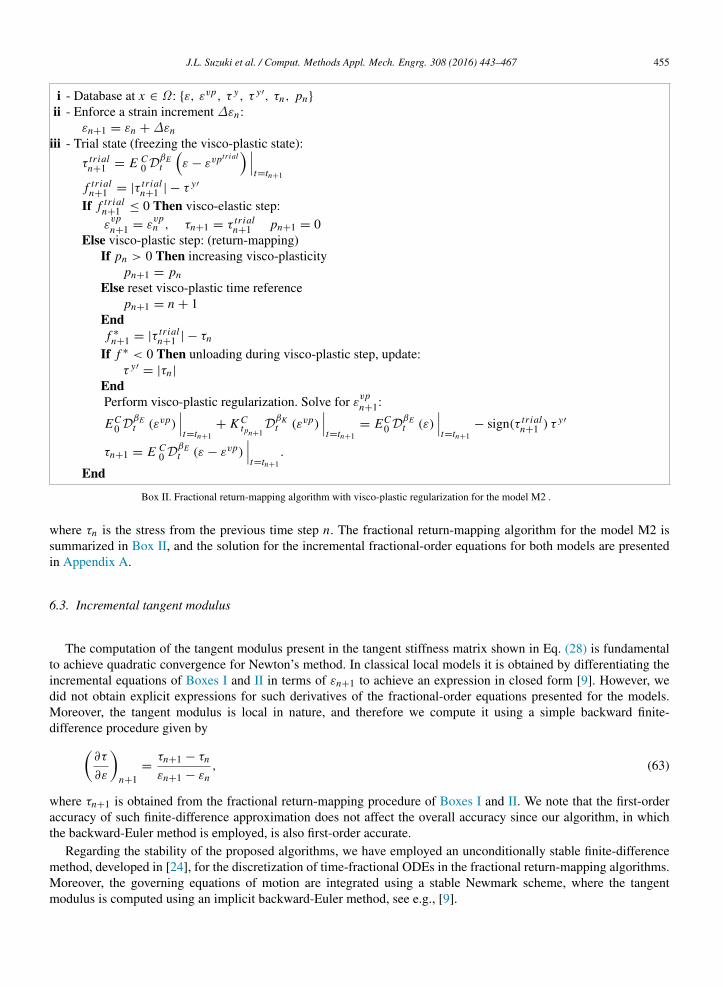
where τn is the stress from the previous time step n. The fractional return-mapping algorithm for the model M2 issummarized in Box II, and the solution for the incremental fractional-order equations for both models are presentedin Appendix A.

6.3. Incremental tangent modulus

The computation of the tangent modulus present in the tangent stiffness matrix shown in Eq. (28) is fundamentalto achieve quadratic convergence for Newton’s method. In classical local models it is obtained by differentiating theincremental equations of Boxes I and II in terms of εn+1 to achieve an expression in closed form [9]. However, wedid not obtain explicit expressions for such derivatives of the fractional-order equations presented for the models.Moreover, the tangent modulus is local in nature, and therefore we compute it using a simple backward finite-difference procedure given by

∂τ

∂ε

n+1

=τn+1 − τn

εn+1 − εn, (63)

where τn+1 is obtained from the fractional return-mapping procedure of Boxes I and II. We note that the first-orderaccuracy of such finite-difference approximation does not affect the overall accuracy since our algorithm, in whichthe backward-Euler method is employed, is also first-order accurate.

Regarding the stability of the proposed algorithms, we have employed an unconditionally stable finite-differencemethod, developed in [24], for the discretization of time-fractional ODEs in the fractional return-mapping algorithms.Moreover, the governing equations of motion are integrated using a stable Newmark scheme, where the tangentmodulus is computed using an implicit backward-Euler method, see e.g., [9].


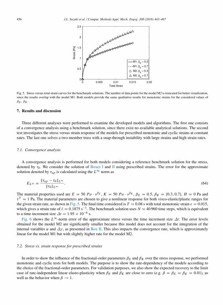
Fig. 5. Stress versus total strain curves for the benchmark solutions. The number of data points for the model M2 is truncated for better visualization,since the results overlap with the model M1. Both models provide the same qualitative results for monotonic strains for the considered values ofβE , βK .

7. Results and discussion

Three different analyses were performed to examine the developed models and algorithms. The first one consistsof a convergence analysis using a benchmark solution, since there exist no available analytical solutions. The secondtest investigates the stress versus strain response of the models for prescribed monotonic and cyclic strains at constantrates. The last one solves a two-member truss with a snap-through instability with large strains and high strain rates.

7.1. Convergence analysis

A convergence analysis is performed for both models considering a reference benchmark solution for the stress,denoted by τb. We consider the solution of Boxes I and II using prescribed strains. The error for the approximatesolution denoted by τap is calculated using the L∞ norm as

EL∞ =∥τap − τb∥L∞

∥τb∥L∞

. (64)

The material properties used are E = 50 Pa · sβE , K = 50 Pa · sβK , βE = 0.5, βK = 0.3, 0.7, H = 0 Pa andτY

= 1 Pa. The material parameters are chosen to give a nonlinear response for both visco-elastic/plastic ranges forthe given strain rate, as shown in Fig. 5. The final time considered is T = 0.08 s with total monotonic strain ε = 0.015,which gives a strain rate of ε = 0.1875 s−1. The benchmark solution uses N = 40 960 time steps, which is equivalentto a time increment size ∆t = 1.95 × 10−6 s.

Fig. 6 shows the L∞-norm error of the approximate stress versus the time increment size ∆t . The error levelsobtained for the model M2 are significantly smaller because this model does not account for the integration of theinternal variables α and ∆γ , as presented in Box II. This also impacts the convergence rate, which is approximatelylinear for the model M1 but with slightly higher rate for the model M2.

7.2. Stress vs. strain response for prescribed strains

In order to show the influence of the fractional-order parameters βE and βK over the stress response, we performedmonotonic and cyclic tests for both models. The purpose is to show the rate-dependency of the models according tothe choice of the fractional-order parameters. For validation purposes, we also show the expected recovery to the limitcase of rate-independent linear elasto-plasticity when βE and βK are close to zero (e.g. β = βE = βK = 0.01), aswell as the behavior when β → 1.


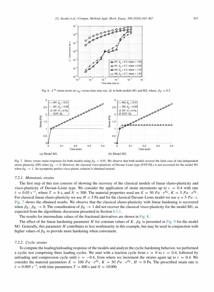
Fig. 6. L∞-norm errors in τap versus time step size ∆t in both models M1 and M2, where, βE = 0.5.

(a) Model M1. (b) Model M2.

Fig. 7. Stress versus strain responses for both models using βE = 0.01. We observe that both models recover the limit case of rate-independentelasto-plasticity (EP) when βK → 0. However, the classical visco-plasticity of Duvaut–Lions type (EVP-DL) is not recovered for the model M1when βK → 1. An asymptotic perfect visco-plastic solution is obtained instead.

7.2.1. Monotonic strainsThe first step of this test consists of showing the recovery of the classical models of linear elasto-plasticity and

visco-plasticity of Duvaut–Lions type. We consider the application of strain increments up to ε = 0.4 with rateε = 0.05 s−1, where T = 8 s, and N = 500. The material properties used are E = 50 Pa · sβE , K = 5 Pa · sβK .For classical linear elasto-plasticity we use H = 5 Pa and for the classical Duvaut–Lions model we use η = 5 Pa · s.Fig. 7 shows the obtained results. We observe that the classical elasto-plasticity with linear hardening is recoveredwhen βE , βK → 0. The consideration of βK → 1 did not recover the classical visco-plasticity for the model M1, asexpected from the algorithmic discussion presented in Section 6.1.1.

The results for intermediate values of the fractional derivatives are shown in Fig. 8.The effect of the linear hardening parameter H for constant values of K , βK is presented in Fig. 9 for the model

M1. Generally, this parameter H contributes to less nonlinearity in this example, but may be used in conjunction withhigher values of βK to provide more hardening when convenient.

7.2.2. Cyclic strainsTo compute the loading/unloading response of the models and analyze the cyclic hardening behavior, we performed

a cyclic test comprising three loading cycles. We start with a traction cycle from ε = 0 to ε = 0.4, followed byunloading and compression cycle until ε = −0.4, from where we increment the strains again up to ε = 0.4. Weconsider the material parameters E = 100 Pa · sβE , K = 50 Pa · sβK , H = 0 Pa. The prescribed strain rate isε = 0.005 s−1, with time parameters T = 400 s and N = 10 000.



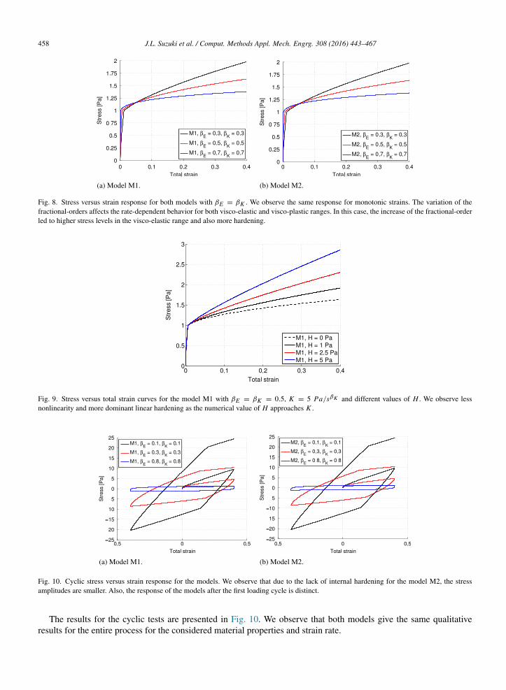
Fig. 8. Stress versus strain response for both models with βE = βK . We observe the same response for monotonic strains. The variation of thefractional-orders affects the rate-dependent behavior for both visco-elastic and visco-plastic ranges. In this case, the increase of the fractional-orderled to higher stress levels in the visco-elastic range and also more hardening.

Fig. 9. Stress versus total strain curves for the model M1 with βE = βK = 0.5, K = 5 Pa/sβK and different values of H . We observe lessnonlinearity and more dominant linear hardening as the numerical value of H approaches K .


Fig. 10. Cyclic stress versus strain response for the models. We observe that due to the lack of internal hardening for the model M2, the stressamplitudes are smaller. Also, the response of the models after the first loading cycle is distinct.

The results for the cyclic tests are presented in Fig. 10. We observe that both models give the same qualitativeresults for the entire process for the considered material properties and strain rate.


(a) K/E = 0.1 s0.799. (b) K/E = 0.5 s0.799.

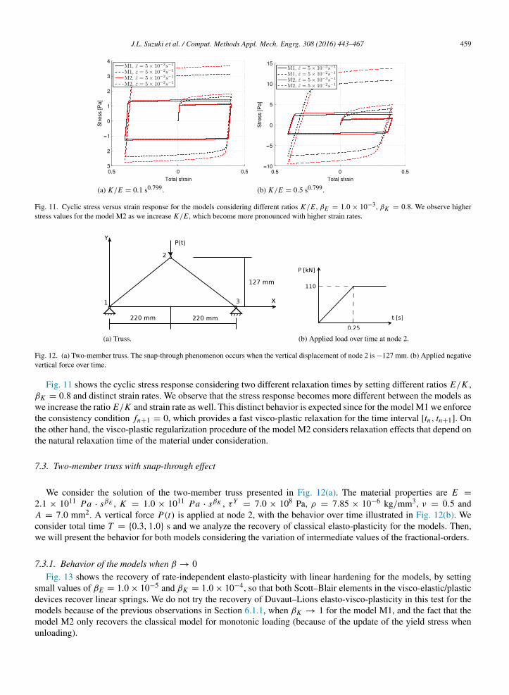
Fig. 11. Cyclic stress versus strain response for the models considering different ratios K/E , βE = 1.0 × 10−3, βK = 0.8. We observe higherstress values for the model M2 as we increase K/E , which become more pronounced with higher strain rates.

(a) Truss. (b) Applied load over time at node 2.

Fig. 12. (a) Two-member truss. The snap-through phenomenon occurs when the vertical displacement of node 2 is −127 mm. (b) Applied negativevertical force over time.

Fig. 11 shows the cyclic stress response considering two different relaxation times by setting different ratios E/K ,βK = 0.8 and distinct strain rates. We observe that the stress response becomes more different between the models aswe increase the ratio E/K and strain rate as well. This distinct behavior is expected since for the model M1 we enforcethe consistency condition fn+1 = 0, which provides a fast visco-plastic relaxation for the time interval [tn, tn+1]. Onthe other hand, the visco-plastic regularization procedure of the model M2 considers relaxation effects that depend onthe natural relaxation time of the material under consideration.

7.3. Two-member truss with snap-through effect

We consider the solution of the two-member truss presented in Fig. 12(a). The material properties are E =

2.1 × 1011 Pa · sβE , K = 1.0 × 1011 Pa · sβK , τY= 7.0 × 108 Pa, ρ = 7.85 × 10−6 kg/mm3, ν = 0.5 and

A = 7.0 mm2. A vertical force P(t) is applied at node 2, with the behavior over time illustrated in Fig. 12(b). Weconsider total time T = 0.3, 1.0 s and we analyze the recovery of classical elasto-plasticity for the models. Then,we will present the behavior for both models considering the variation of intermediate values of the fractional-orders.

7.3.1. Behavior of the models when β → 0Fig. 13 shows the recovery of rate-independent elasto-plasticity with linear hardening for the models, by setting

small values of βE = 1.0 × 10−5 and βK = 1.0 × 10−4, so that both Scott–Blair elements in the visco-elastic/plasticdevices recover linear springs. We do not try the recovery of Duvaut–Lions elasto-visco-plasticity in this test for themodels because of the previous observations in Section 6.1.1, when βK → 1 for the model M1, and the fact that themodel M2 only recovers the classical model for monotonic loading (because of the update of the yield stress whenunloading).


(a) Displacement versus time. (b) Stress versus strain.

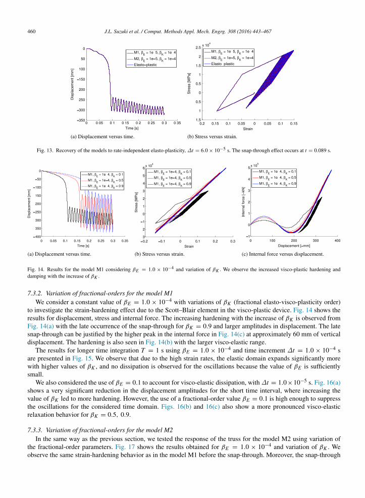
Fig. 13. Recovery of the models to rate-independent elasto-plasticity, ∆t = 6.0 × 10−5 s. The snap-through effect occurs at t = 0.089 s.

(a) Displacement versus time. (b) Stress versus strain. (c) Internal force versus displacement.

Fig. 14. Results for the model M1 considering βE = 1.0 × 10−4 and variation of βK . We observe the increased visco-plastic hardening anddamping with the increase of βK .

7.3.2. Variation of fractional-orders for the model M1We consider a constant value of βE = 1.0 × 10−4 with variations of βK (fractional elasto-visco-plasticity order)

to investigate the strain-hardening effect due to the Scott–Blair element in the visco-plastic device. Fig. 14 shows theresults for displacement, stress and internal force. The increasing hardening with the increase of βK is observed fromFig. 14(a) with the late occurrence of the snap-through for βK = 0.9 and larger amplitudes in displacement. The latesnap-through can be justified by the higher peak in the internal force in Fig. 14(c) at approximately 60 mm of verticaldisplacement. The hardening is also seen in Fig. 14(b) with the larger visco-elastic range.

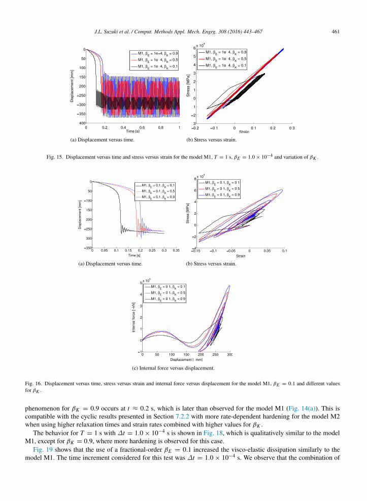
The results for longer time integration T = 1 s using βE = 1.0 × 10−4 and time increment ∆t = 1.0 × 10−4 sare presented in Fig. 15. We observe that due to the high strain rates, the elastic domain expands significantly morewith higher values of βK , and no dissipation is observed for the oscillations because the value of βE is sufficientlysmall.

We also considered the use of βE = 0.1 to account for visco-elastic dissipation, with ∆t = 1.0×10−5 s. Fig. 16(a)shows a very significant reduction in the displacement amplitudes for the short time interval, where increasing thevalue of βK led to more hardening. However, the use of a fractional-order value βE = 0.1 is high enough to suppressthe oscillations for the considered time domain. Figs. 16(b) and 16(c) also show a more pronounced visco-elasticrelaxation behavior for βK = 0.5, 0.9.

7.3.3. Variation of fractional-orders for the model M2In the same way as the previous section, we tested the response of the truss for the model M2 using variation of

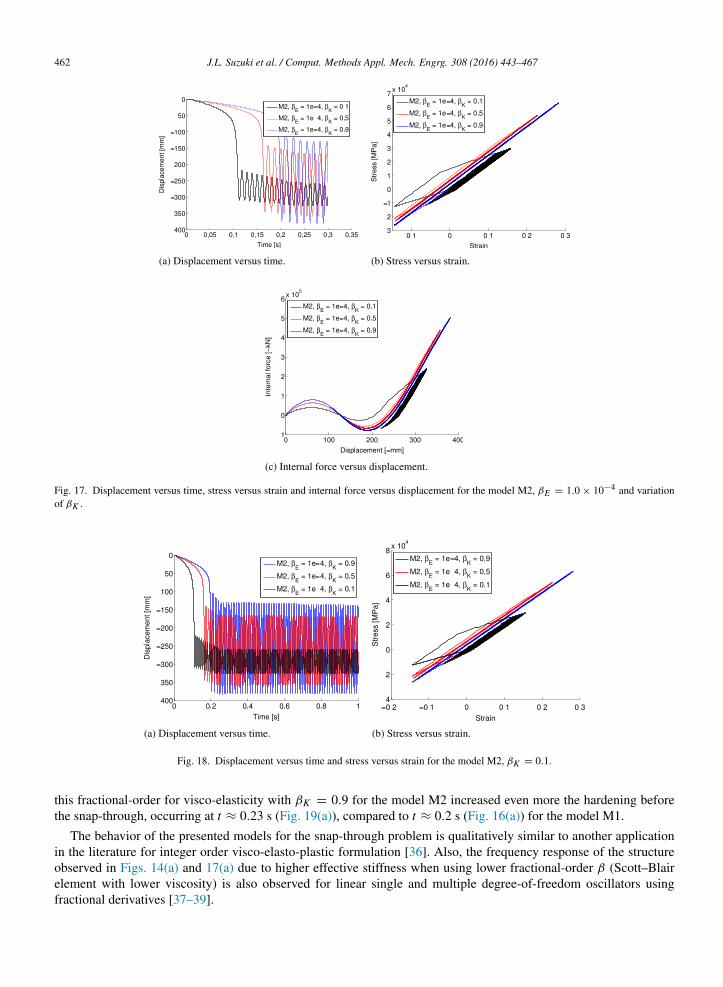
the fractional-order parameters. Fig. 17 shows the results obtained for βE = 1.0 × 10−4 and variation of βK . Weobserve the same strain-hardening behavior as in the model M1 before the snap-through. Moreover, the snap-through



Fig. 15. Displacement versus time and stress versus strain for the model M1, T = 1 s, βE = 1.0 × 10−4 and variation of βK .


(c) Internal force versus displacement.

Fig. 16. Displacement versus time, stress versus strain and internal force versus displacement for the model M1, βE = 0.1 and different valuesfor βK .

phenomenon for βK = 0.9 occurs at t ≈ 0.2 s, which is later than observed for the model M1 (Fig. 14(a)). This iscompatible with the cyclic results presented in Section 7.2.2 with more rate-dependent hardening for the model M2when using higher relaxation times and strain rates combined with higher values for βK .

The behavior for T = 1 s with ∆t = 1.0 × 10−4 s is shown in Fig. 18, which is qualitatively similar to the modelM1, except for βK = 0.9, where more hardening is observed for this case.

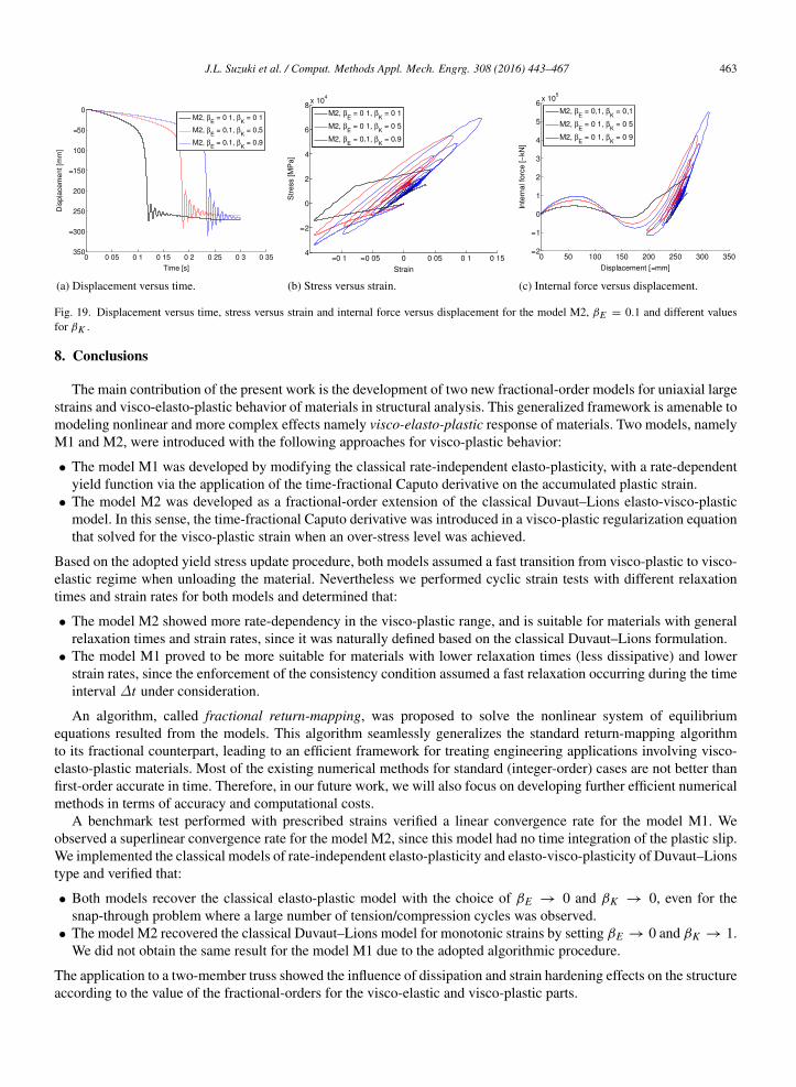
Fig. 19 shows that the use of a fractional-order βE = 0.1 increased the visco-elastic dissipation similarly to themodel M1. The time increment considered for this test was ∆t = 1.0 × 10−4 s. We observe that the combination of



(c) Internal force versus displacement.

Fig. 17. Displacement versus time, stress versus strain and internal force versus displacement for the model M2, βE = 1.0 × 10−4 and variationof βK .


Fig. 18. Displacement versus time and stress versus strain for the model M2, βK = 0.1.

this fractional-order for visco-elasticity with βK = 0.9 for the model M2 increased even more the hardening beforethe snap-through, occurring at t ≈ 0.23 s (Fig. 19(a)), compared to t ≈ 0.2 s (Fig. 16(a)) for the model M1.

The behavior of the presented models for the snap-through problem is qualitatively similar to another applicationin the literature for integer order visco-elasto-plastic formulation [36]. Also, the frequency response of the structureobserved in Figs. 14(a) and 17(a) due to higher effective stiffness when using lower fractional-order β (Scott–Blairelement with lower viscosity) is also observed for linear single and multiple degree-of-freedom oscillators usingfractional derivatives [37–39].


(a) Displacement versus time. (b) Stress versus strain. (c) Internal force versus displacement.

Fig. 19. Displacement versus time, stress versus strain and internal force versus displacement for the model M2, βE = 0.1 and different valuesfor βK .

8. Conclusions

The main contribution of the present work is the development of two new fractional-order models for uniaxial largestrains and visco-elasto-plastic behavior of materials in structural analysis. This generalized framework is amenable tomodeling nonlinear and more complex effects namely visco-elasto-plastic response of materials. Two models, namelyM1 and M2, were introduced with the following approaches for visco-plastic behavior:

• The model M1 was developed by modifying the classical rate-independent elasto-plasticity, with a rate-dependentyield function via the application of the time-fractional Caputo derivative on the accumulated plastic strain.

• The model M2 was developed as a fractional-order extension of the classical Duvaut–Lions elasto-visco-plasticmodel. In this sense, the time-fractional Caputo derivative was introduced in a visco-plastic regularization equationthat solved for the visco-plastic strain when an over-stress level was achieved.

Based on the adopted yield stress update procedure, both models assumed a fast transition from visco-plastic to visco-elastic regime when unloading the material. Nevertheless we performed cyclic strain tests with different relaxationtimes and strain rates for both models and determined that:

• The model M2 showed more rate-dependency in the visco-plastic range, and is suitable for materials with generalrelaxation times and strain rates, since it was naturally defined based on the classical Duvaut–Lions formulation.

• The model M1 proved to be more suitable for materials with lower relaxation times (less dissipative) and lowerstrain rates, since the enforcement of the consistency condition assumed a fast relaxation occurring during the timeinterval ∆t under consideration.

An algorithm, called fractional return-mapping, was proposed to solve the nonlinear system of equilibriumequations resulted from the models. This algorithm seamlessly generalizes the standard return-mapping algorithmto its fractional counterpart, leading to an efficient framework for treating engineering applications involving visco-elasto-plastic materials. Most of the existing numerical methods for standard (integer-order) cases are not better thanfirst-order accurate in time. Therefore, in our future work, we will also focus on developing further efficient numericalmethods in terms of accuracy and computational costs.

A benchmark test performed with prescribed strains verified a linear convergence rate for the model M1. Weobserved a superlinear convergence rate for the model M2, since this model had no time integration of the plastic slip.We implemented the classical models of rate-independent elasto-plasticity and elasto-visco-plasticity of Duvaut–Lionstype and verified that:

• Both models recover the classical elasto-plastic model with the choice of βE → 0 and βK → 0, even for thesnap-through problem where a large number of tension/compression cycles was observed.

• The model M2 recovered the classical Duvaut–Lions model for monotonic strains by setting βE → 0 and βK → 1.We did not obtain the same result for the model M1 due to the adopted algorithmic procedure.

The application to a two-member truss showed the influence of dissipation and strain hardening effects on the structureaccording to the value of the fractional-orders for the visco-elastic and visco-plastic parts.


The developed models can be fitted to experimental data from uniaxial stress/strain tests at constant or varyingstrain rates, as well as creep and relaxation tests, in order to identify the corresponding material coefficients andfractional-orders. Although the visco-elastic portion of the models consisted of a single Scott–Blair element, a moresophisticated fractional-order model can be incorporated (e.g. Kelvin–Voigt, Zener [40]).

In the case of very large visco-elastic strains (e.g. rubber), a hyper-visco-elastic behavior should be incorporatedto the models to provide an accurate description. Moreover, the accuracy of the developed models can be improvedby using a higher-order time integration method (e.g. fast convolution [41]). However, more theoretical developmentswould be necessary to derive the constitutive equations in convolution form. Also, a higher-order method to estimatethe algorithmic tangent modulus would also be required (e.g. complex-step derivative [42]), since the finite-differencemethod adopted here was first-order accurate. Moreover, an extension of the developed models can be done in astraightforward way to account for kinematic hardening effects, as well as a continuum damage model (e.g. Lemaitre’smodel [43]).

Therefore, fractional-order constitutive relations like the models developed in this work may be suitable to describethe constitutive behavior of a range of applications like: polymers, glass, metal alloys at higher temperatures [44],biological tissues (e.g. skin, bone, respiratory tissue, tendons [45–49]), as well as other relaxation phenomena in chem-istry, electronics, magnetic systems [50,44,51] and social sciences (e.g. memory phenomena in psychology [52]).

Acknowledgments

This work was supported by the Coordination for the Improvement of Higher Education Personnel (CAPES), grantnumber 99999.010717/2014-05, the MURI/ARO on “Fractional PDEs for Conservation Laws and Beyond: Theory,Numerics and Applications (W911NF-15-1-0562)”, and the University of Campinas (UNICAMP) (33003017).

Appendix A. Solution of the fractional-order differential equations in incremental form

In this section we present the explicit expressions for the variables at time tn+1 after applying the finite-differencescheme for the Caputo time-fractional derivatives for both models. The trial stress is given by

τ tr ialn+1 = E∗

εn+1 − εn + HβE ε − ε

vptr ial

n+1 + εvpn − HβE εvp

, (A.1)

where

E∗=

E

∆t βE Γ (2 − βE ), (A.2)

where E∗ has units of [Pa]. Recalling that εvptr ial

n+1 = εvpn , we can rewrite Eq. (A.1) as

τ tr ialn+1 = E∗

εn+1 − εn + HβE ε − HβE εvp . (A.3)

The associated trial yield function for the model M1 is explicitly given by


n+1 | −

τY

+ Hαtr ialn+1 + K ∗(αtr ial

n+1 − αn + HβKtpn

α), (A.4)

with

K ∗=

K

∆t βK Γ (2 − βK ), (A.5)

where K∗ has units of [Pa]. Recalling that αtr ialn+1 = αn , we obtain


n+1 | −

τY

+ Hαn + K ∗HβKtpn

α

. (A.6)

Now we consider the solution for the plastic slip ∆γn+1. Applying Eqs. (44) and (49) to Eq. (43) for the model M1,we obtain

E

∆t βE Γ (2 − βE )

∆γn+1 − ∆γn + HβE ∆γ

+

K

∆t βK Γ (2 − βK )

∆γn+1 − ∆γn + HβK

tpn+1∆γ


+ H∆γn+1 = f tr ialn+1 . (A.7)

Solving the above equation for the plastic slip at current time tn+1, we obtain

∆γn+1 =

E∗∆γn − HβE ∆γ

+ K ∗

∆γn − HβK

tpn+1∆γ

+ f tr ial

n+1

E∗ + K ∗ + H. (A.8)

Applying the same procedure to Eq. (38), we obtain the updated stress τn+1 for the model M1 given by

τn+1 = τ tr ialn+1 − E∗

∆γn+1 − ∆γn + HβE ∆γ

sign

τ tr ial

n+1

. (A.9)

Now we present the explicit expression for εvpn+1 from Eq. (61) for the model M2. Therefore, we have

E∗εvpn+1 − ε

vpn + HβE εvp

+ K ∗

εvpn+1 − ε

vpn + HβK

tpn+1εvp

= E∗

εn+1 − εn + HβE ε

− sign

τ tr ial

n+1

τ y′. (A.10)

Solving for εvpn+1, we obtain

εvpn+1 = ε

vpn +

E∗εn+1 − εn + HβE ε − HβK ε

− K ∗HβK

tpn+1εvp

− signτ tr ial

n+1

τ y′

E∗ + K ∗. (A.11)

Appendix B. Newmark integration scheme

We consider the equation of conservation of linear momentum in the discrete implicit form using a Newmarkintegration scheme without damping effects [35],

Man+1 + Rn+1 = Pn+1, (B.1)

with the above terms already described in Section 5. The initial conditions at t = 0 are given by

u0 = u, v0 = v. (B.2)

The global accelerations and velocities are approximated as

an+1 = b1 (un+1 − un) − b2vn − b3an (B.3)

vn+1 = b4 (un+1 − un) − b5vn − b6an, (B.4)

with the following Newmark coefficients

b1 =1

g1∆t2 , b2 =1

g1∆t, b3 =

1 − 2g1

2g1

b4 =g2

g1∆t2 , b5 =

1 −

g2

g1

, b6 =

1 −

g2

2g1

∆t,

where it is usual to choose g1 = 0.5, g2 = 0.25 for unconditional stability.

References

[1] F. Mainardi, Fractional Calculus and Waves in Linear Viscoelasticity: An Introduction to Mathematical Models, Imperial College Press, 2010.[2] B.J. West, M. Bologna, P. Grigolini, Physics of Fractal Operators, Springer Verlag, New York, NY, 2003.[3] M. Naghibolhosseini, Estimation of outer-middle ear transmission using DPOAEs and fractional-order modeling of human middle ear (Ph.D.

thesis), City University of New York, NY, 2015.[4] M. Ichise, Y. Nagayanagi, T. Kojima, An analog simulation of non-integer order transfer functions for analysis of electrode processes,

J. Electroanal. Chem. Interfacial Electrochem. 33 (2) (1971) 253–265.[5] D.A. Benson, S.W. Wheatcraft, M.M. Meerschaert, Application of a fractional advection–dispersion equation, Water Resour. Res. 36 (6)

(2000) 1403–1412.

http://refhub.elsevier.com/S0045-7825(16)30441-8/sbref1






[6] R. Metzler, J. Klafter, The random walk’s guide to anomalous diffusion: a fractional dynamics approach, Phys. Rep. 339 (1) (2000) 1–77.[7] R. Klages, G. Radons, I.M. Sokolov, Anomalous Transport: Foundations and Applications, Wiley-VCH, 2008.[8] J. Bonet, R. Wood, Nonlinear Continuum Mechanics for Finite Element Analysis, second ed., Cambridge, 2008.[9] J. Simo, T. Hughes, Computational Inelasticity, Springer-Verlag, 1998.

[10] W. Sumelka, Fractional viscoplasticity, in: 37th Solid Mechanics Conference, Warsaw, Poland, 2012, pp. 102–103.[11] W. Sumelka, Fractional viscoplasticity: an introduction, in: Workshop 2012—Dynamic Behavior of Materials and Safety of Structures,

Poznan, Poland, 2012, pp. 1–2.[12] W. Sumelka, Fractional viscoplasticity, Mech. Res. Commun. 56 (2014) 31–36.[13] P. Perzyna, The Constitutive Equations for Rate Sensitive Plastic Materials, Tech. Report, DTIC Document, 1962.[14] W. Sumelka, Application of fractional continuum mechanics to rate independent plasticity, Acta Mech. 225 (11) (2014) 3247–3264.[15] C. Lubich, On the stability of linear multistep methods for Volterra convolution equations, IMA J. Numer. Anal. 3 (4) (1983) 439–465.[16] C. Lubich, Discretized fractional calculus, SIAM J. Math. Anal. 17 (3) (1986) 704–719.[17] J. Sanz-Serna, A numerical method for a partial integro-differential equation, SIAM J. Numer. Anal. 25 (2) (1988) 319–327.[18] N. Sugimoto, Burgers equation with a fractional derivative; hereditary effects on nonlinear acoustic waves, J. Fluid Mech. 225 (631–653)

(1991) 4.[19] R. Gorenflo, F. Mainardi, D. Moretti, P. Paradisi, Time fractional diffusion: a discrete random walk approach, Nonlinear Dynam. 29 (1–4)

(2002) 129–143.[20] K. Diethelm, N.J. Ford, Analysis of fractional differential equations, J. Math. Anal. Appl. 265 (2) (2002) 229–248.[21] K. Diethelm, N.J. Ford, A.D. Freed, Detailed error analysis for a fractional adams method, Numer. Algorithms 36 (1) (2004) 31–52.[22] T. Langlands, B. Henry, The accuracy and stability of an implicit solution method for the fractional diffusion equation, J. Comput. Phys. 205

(2) (2005) 719–736.[23] Z.-Z. Sun, X. Wu, A fully discrete difference scheme for a diffusion-wave system, Appl. Numer. Math. 56 (2) (2006) 193–209.[24] Y. Lin, C. Xu, Finite difference/spectral approximations for the time-fractional diffusion equation, J. Comput. Phys. 225 (2) (2007) 1533–1552.[25] M. Zayernouri, W. Cao, Z. Zhang, G.E. Karniadakis, Spectral and discontinuous spectral element methods for fractional delay equations,

SIAM J. Sci. Comput. 36 (6) (2014) B904–B929.[26] M. Zayernouri, G.E. Karniadakis, Exponentially accurate spectral and spectral element methods for fractional ODEs, J. Comput. Phys. 257

(2014) 460–480.[27] M. Zayernouri, M. Ainsworth, G.E. Karniadakis, A unified Petrov–Galerkin spectral method for fractional PDEs, Comput. Methods Appl.

Mech. Eng. 283 (2015) 1545–1569.[28] M. Zayernouri, G.E. Karniadakis, Fractional spectral collocation methods for linear and nonlinear variable order FPDEs, J. Comput. Phys.

(Special issue on FPDEs: Theory, Numerics, and Applications) 293 (2015) 312–338.[29] M. Zayernouri, T. Matzavinos, Fractional Adams- Bashforth/Moulton methods: An application to the fractional Keller–Segel chemotaxis

system, J. Comput. Phys. 317 (2016) 1–14.[30] Z.-J. Fu, W. Chen, H.-T. Yang, Boundary particle method for Laplace transformed time fractional diffusion equations, J. Comput. Phys. 235

(2013) 52–66.[31] G. Pang, W. Chen, Z. Fu, Space-fractional advection–dispersion equations by the Kansa method, J. Comput. Phys. 293 (2015) 280–296.[32] W. Chen, G. Pang, A new definition of fractional Laplacian with application to modeling three-dimensional nonlocal heat conduction,

J. Comput. Phys. 309 (2016) 350–367.[33] I. Podlubny, Fractional Differential Equations, Academic Press, San Diego, CA, USA, 1999.[34] M. Bittencourt, Computational Solid Mechanics: Variational Formulation and High Order Approximation, CRC Press, 2014.[35] P. Wriggers, Nonlinear Finite Element Methods, Springer, 2008.[36] T. Carniel, P. Muoz Rojas, M. Vaz Jr., A viscoelastic viscoplastic constitutive model including mechanical degradation: Uniaxial transient

finite element formulation at finite strains and application to space truss structures, Appl. Math. Model. 39 (2015) 1725–1739.[37] D. Ingman, J. Suzdalnitsky, Iteration method for equation of viscoelastic motion with fractional differential operator of damping, Comput.

Methods Appl. Mech. Eng. 190 (37–38) (2001) 5027–5036.[38] D. Ingman, J. Suzdalnitsky, Control of damping oscillations by fractional differential operator with time-dependent order, Comput. Methods

Appl. Mech. Eng. 193 (52) (2004) 5585–5595.[39] Y. Shen, S. Yang, H. Xing, H. Ma, Primary resonance of Duffing oscillator with two kinds of fractional-order derivatives, Int. J. Non-Linear

Mech. 47 (2012) 975–983.[40] S. Nasholm, S. Holm, On a fractional Zener elastic wave equation, Fract. Calc. Appl. Anal. 16 (1) (2013) 26–50.[41] C. Lubich, A. Schadle, Fast convolution for nonreflecting boundary conditions, SIAM J. Sci. Comput. 24 (2002) 161–182.[42] M. Tanaka, M. Fujikawa, D. Balzani, J. Schroder, Robust numerical calculation of tangent moduli at finite strains based on complex-step

derivative approximation and its application to localization analysis, Comput. Methods Appl. Mech. Engrg. 269 (2014) 454–470.[43] J. Lemaitre, Coupled elasto-plasticity and damage constitutive equations, Comput. Methods Appl. Mech. Engrg. 51 (1) (1985) 31–49.[44] K. Ngai, Relaxation and Diffusion in Complex Systems, Springer, 2011.[45] B. Querleux, Computational Biophysics of the Skin, CRC Press, 2014.[46] J. Weickenmeier, M. Jabareen, Elastic–viscoplastic modeling of soft biological tissues using a mixed finite element formulation based on the

relative deformation gradient, Int. J. Numer. Methods Biomed. Eng. 30 (11) (2014) 1238–1262.[47] J. Schwiedrzik, P. Zysset, An anisotropic elastic-viscoplastic damage model for bone tissue, Biomech. Model. Mechanobiol. 12 (2) (2013)

201–213.[48] J. Sun, Y. Tsuang, T. Liu, Y. Hang, C. Cheng, W. Lee, Viscoplasticity of rabbit skeletal muscle under dynamic cyclic loading, Clin. Biomech.

10 (5) (1995) 258–262.












































[49] P. Romero, C. Caete, J. Aguilar, F. Romero, Elasticity, viscosity and plasticity in lung parenchyma, in: J. Milic-Emili (Ed.), Applied Physiologyin Respiratory Mechanics, Topics in Anaesthesia and Critical Care, Springer Milan, 1998, pp. 57–72.

[50] F. Mainardi, R. Gorenflo, Time-fractional derivatives in relaxation processes: a tutorial survey, Fract. Calc. Appl. Anal. 10 (3) (2007) 269–308.[51] C. Monje, Y. Chen, B. Vinagre, D. Xue, V. Feliu-Batlle, Fractional-order Systems and Controls, Springer, 2010.[52] M. Du, Z. Wang, H. Hu, Measuring memory with the order of fractional derivative, Sci. Rep. 3 (3431) (2013) 1–3.





Fractional-order uniaxial visco-elasto-plastic models … · Fractional-order uniaxial...

Documents

Transcript of Fractional-order uniaxial visco-elasto-plastic models … · Fractional-order uniaxial...