FRACTIONAL MAGNETOHYDRODYNAMICS …...FRACTIONAL MAGNETOHYDRODYNAMICS OLDROYD-B FLUID OVER AN...

FRACTIONAL MAGNETOHYDRODYNAMICS OLDROYD-B FLUIDOVER AN OSCILLATING PLATE

by

Muhammad JAMIL a,b*, Najeeb Alam KHAN c, and Nazish SHAHID a

a Abdus Salam School of Mathematical Sciences,GC University, Lahore, Pakistanb Department of Mathematics, NED University of Engineering and Technology, Karachi,Pakistan

c Department of Mathematics, University of Karachi, Karachi, Pakistan

Original scientific paperDOI: 10.2298/110731140J

This paper presents some new exact solutions corresponding to the oscillatingflows of a magnetohydrodynamic Oldroyd-B fluid with fractional derivatives. Thefractional calculus approach in the governing equations is used. The exact solu-tions for the oscillating motions of a fractional magnetohydrodynamic Oldroyd-Bfluid due to sine and cosine oscillations of an infinite plate are established with thehelp of discrete Laplace transform. The expressions for velocity field and the asso-ciated shear stress that have been obtained, presented in series form in terms of FoxH-functions, satisfy all imposed initial and boundary conditions. Similar solutionsfor ordinary magnetohydrodynamic Oldroyd-B, fractional and ordinarymagnetohydrodynamic Maxwell, fractional and ordinary magnetohydrodynamicsecond grade and magnetohydrodynamic Newtonian fluid as well as those for hy-drodynamic fluids are obtained as special cases of general solutions. Finally, theobtained solutions are graphically analyzed through various parameters of inter-est.Mathematics Subject Classification (2010). 76A05, 76A10

Key words: magnetohydrodynamic Oldroyd-B fluid, fractional derivatives,oscillating flows, exact solutions, Fox H-functions, velocity field,shear stress, discrete laplace transforms.

Introduction

Flows in the neighborhood of spinning or oscillating bodies are of interest to both aca-

demic field and industry. The study of time-dependent flows of viscoelastic fluids caused by the

oscillations of a flat plate is of considerable interest both industrially as well as a test to assess

the performance of numerical methods for the computation of transient flows. Such flows are

not only of fundamental and theoretical interest but they also occur in many biological and in-

dustrial processes such as the quasi-periodic blood flow in the cardiovascular system, acoustic

streaming around an oscillating body, an unsteady boundary layer with fluctuations and so forth.

Although exact solutions to various oscillating flow problems of Newtonian fluid have been ob-

tained and are available in the literature, the first closed-form transient solution for the flow of a

Newtonian fluid due to an oscillating plate seems to be that of Penton [1]. Puri and Kythe [2]

have discussed an unsteady flow problem which deals with non-classical heat condition effects

and the structure of waves in Stokes' second problem. Erdogan [3] provided two starting solu-

tions for the motion of a viscous fluid due to cosine and sine oscillations of a flat plate. The first

exact solutions for the longitudinal and torsional oscillations of a rod in a non-Newtonian fluid

Jamil, M., et al.: Fractional Magnetohydrodynamics Oldroyd-B Fluid over an ...THERMAL SCIENCE: Year 2013, Vol. 17, No. 4, pp. 997-1011 997

* Corresponding author; e-mail: [email protected]

are those obtained by Rajagopal [4] and Rajagopal and Bhatnagar [5]. Moreover, exact solu-

tions for various flow geometries in non-Newtonian fluids have been also obtained by Hayat et

al. [6], Aksel et al. [7], Khan et al. [8], and Fetecau et al. [9, 10]. More recently exact solutions

for oscillating flow of different non-Newtonian fluids have been obtained by Khan et al. [11,

12], Mahmood et al. [13], Zhen et al. [14], and Anjum et al. [15].

These exact solutions become even rare if the constitutive equations of non-Newto-

nian fluids with fractional derivatives are considered. For numerous fluids between elastic and

viscous materials the fractional constitutive relationship model has an advantage over the cus-

tomary constitutive relationship model. Fractional calculus has achieved much success in the

description of the complex dynamics. The constitutive equations with fractional derivatives

have been proved to be a valuable tool to handle viscoelastic properties [16]. In [17], the rest

state stability of an objective fractional derivative viscoelastic fluid model has been established

which is an important finding that gives strength to the physical basis of these fractional models.

Moreover, a very good fit of experimental data is achieved when the constitutive equation with

fractional derivatives is used [18]. We mention here some recent contributions [19-35] in the

discussion of flows of viscoelastic fluids with a fractional calculus approach.

The aim of this communication is two fold. Firstly, it is to give new exact solutions for

magnetohydrodynamic (MHD) Oldroyd-B fluids with fractional derivatives, which is more nat-

ural and appropriate tool to describe the complex behavior of non-Newtonian fluids. Secondly,

it is to study the oscillating effects on MHD Oldroyd-B fluids with fractional derivatives, which

is important due to their practical applications. More precisely, our aim is to find the velocity

field and the shear stress corresponding to the motion of fractional MHD Oldroyd-B fluid due to

a plate that oscillates with sine or cosine oscillations in its own plane. The general solutions are

obtained using the discrete Laplace transform formula for sequential fractional derivatives.

They are presented in series form in terms of the Fox H-functions. The similar solutions for ordi-

nary MHD Oldroyd-B, fractional and ordinary MHD Maxwell, fractional and ordinary MHD

second grade and MHD Newtonian fluids, can easily be obtained as special cases of general so-

lutions. Furthermore, the solutions for hydrodynamic fluids are also easily obtained from gen-

eral solutions as special cases and they are similar with previously known results in literature.

The general solutions also recover many existing solutions for Stokes' first and second problem

for MHD and ordinary non-Newtonian fluids. Finally, the influence of the material, magnetic

and fractional parameters on the motion of MHD fractional Oldroyd-B fluids is underlined by

graphical illustrations. The difference among fractional MHD Oldroyd-B, fractional MHD

Maxwell, fractional MHD second grade and MHD Newtonian fluid models is also spotlighted.

Basic governing equations

The continuity equation and the equation of motion for the flow of an incompressible

fluid, in the absence of body forces, are:

� � � � � �V T V V0, ( )r r¶

¶

V

t(1)

where r is the fluid density, V – the velocity field, t – the time and � represents the gradient op-

erator. The Cauchy stress T in an incompressible Oldroyd-B fluid is given by

T I S S S LS SL A A LA AL� � � � � � � � � �p Tr

T, ( � ) [ ( � )l m l (2)

where –pI denotes the indeterminate spherical stress due to the constraint of incompressibility, S is

the extra-stress tensor, L – the velocity gradient, A = L + LT – the first Rivlin Ericksen tensor, m –

the dynamic viscosity of the fluid, l and lr are relaxation and retardation times, the superposed dot

Jamil, M., et al.: Fractional Magnetohydrodynamics Oldroyd-B Fluid over an ...998 THERMAL SCIENCE: Year 2013, Vol. 17, No. 4, pp. 997-1011

indicates the material time derivative and the superscript T indicates the transpose operation. The

model characterized by the constitutive eq. (2) contains as special cases the upper-convected

Maxwell model for lr � 0 and the Newtonian fluid model for lr � 0 and l� 0. In some special

flows, as those to be considered here, the governing equations for an Oldroyd-B fluid resemble for

a fluid of second grade. For the problem under consideration we assume a velocity field V and an

extra-stress tensor S of the form:

V = V(y,t) = u(y,t)i, S = S(y,t), (3)

where i is the unit vector along the x-co-ordinate direction. For these flows the constraint of

incompressibility is automatically satisfied. In the absence of a pressure gradient in the x-direc-

tion, the governing equations of the fractional MHD Oldroyd-B fluid are [26]:

( )( , )

( )( , )

(1 1 12

2� � � � �l n l la a b b aD

u y t

tD

u y t

yM Dt r t t

¶

¶

¶

¶

a ) ( , )u y t (4)

( ) ( , ) ( )( , )

1 1� � �l t m la arb bD y t D

u y t

tt t

¶

¶(5)

where t(y, t) = Sxy(y, t) is the non-trivial shear stress, r – the constant density of the fluid, n = m/r

– the kinematic viscosity, M = sB02 /r , s – the electrical conductivity of the fluid, and B0 – the

applied magnetic field [36-38]. Alsoa and b are fractional parameters such that 0 � b < 1 and the

fractional differential operator so called Caputo fractional operator Dtp defined by [39, 40]:

D f t p

f

tp

f t

tp

tp p

t

( ) ( )

( )

( ),

( ),

� �

�

��

�

�

1

10 1

1

0G

t

ttd

d

d

�

�

(6)

where G(.) is the Gamma function. In the following the system of fractional partial differential

eqs. (4) and (5), with appropriate initial and boundary conditions, will be solved by means of

discrete Laplace transform [25-30].

Statement of the problem

Consider an incompressible MHD Oldroyd-B fluid with fractional derivatives occu-

pying the space lying over an infinitely extended plate which is situated in the (x, z) plane and

perpendicular to the y-axis. Initially the fluid, as well as the plate is at rest and at t = 0+ the plate

starts to oscillate in its own plane. Due to the shear, the fluid above the plate is gradually moved.

Its velocity is of the form (3)1 while the governing equations are given by eqs. (4) and (5). The

appropriate initial and boundary conditions are:

u yu y

ty y( , )

( , ), ( , ) ,0

00 0 0 0� � � �

¶

¶t (7)

u y U t UH t t t( , ) sin( ) ( )cos( );0 0� �w wor (8)

where w is the frequency, U – the amplitude of the velocity of the plate and H(.) is the Heaviside

function. Furthermore the natural condition:

u y t y t( , ) � � �0 0as � (9)

has also to be satisfied. It is a consequence of the fact that the fluid is at rest at infinity and there

is no shear in the free stream.


Solution of the problem

Calculation of the velocity field

First of all we solve the velocity field for sine oscillation. Applying the Laplace trans-

form to eq. (4), using the Laplace transform formula for sequential fractional derivatives [39,

40] and taking into account the initial conditions (7) 1,2, we find that:

¶

¶

2

2

1

10

u y q

y

q q M

qu y q

r

( , ) ( )( )

( )( , )�

� �

��

l

n l

a a

b b(10)

The boundary conditions are:

u qU

qu y q y( , ) ( , )0 0

2 2� � �

w

wand as � (11)

where u(y, q) is the Laplace transform of u(y, t) and q is a transform parameter. Solving eqs.

(10) and (11), we get:

u y qU

q

q q M

qy

r

( , ) exp( )( )

( )� �

� �

�

��

�

��

�

w

w

l

n l

a a

b b2 2

1

1 �(12)

In order to obtain u(y, t) = L–1{u(y, q)} and to avoid the lengthy and burdensome calcu-

lations of residues and contour integrals, we apply the discrete inverse Laplace transform

method [25-30]. However, for a suitable presentation of the velocity field, we firstly rewrite eq.

(12) in series form:

u y qU

qU

k

yj

j k

k

( , ) ( )!

(�

��

�

��

�

��

�

� ��

w

ww w

n2 2

2

0 1

1� � M

l m

km

kn

l

l

m

m

)

!

( )

!� ��

��

�

��

��

�

��

�

��

�

��

0 0

12 2

� � la

G G Gk

nk k k

q

rn

k

2

2 2 2

1

�

��

�

��

��

��

�

��

�

��

�

��

�

��

�

��

�

( )

!

lb

G G G 22 20 � � � � ��

�l m n jn a b

�

(13)

Inverting eq. (13) by means of discrete inverse Laplace transform, we find that:

u y t U t Uk

yj

j k

k

( , ) sin( ) ( )!

(� � � �

�

��

�

��

� �� w w w

n

2

0 1

1� � ��

��

��

��

�

�

�

�

� � � � �

�

�

M

l

mt

k

l

l

m

m

kl m j

)

!

( )

!

0

0

22 1

12

�

� la a

G � ��

��

�

��

�

��

�

��

��

�

��

��

��

�

��

G G

G

mk

nk

t

nk

r

n

2 2

2

lb

b

! G G G��

��

�

��

�

��

�

��

�

��

�

��

��

k k kl m n j

n

2 2 22 2

0a b

�

(14)

In terms of the Fox-H function [41], we write the above relation in a simpler form:

u y t U t Uk

y Ms

j

j

kl

( , ) sin( ) ( )!

( )� � � �

�

��

�

��

�

��w w w

n

2

0

1�

l mt

H

l

m

m

kl m j

k

r

!

( )

!

,,

� �

� � � � �

��

��

�

0 0

22 1

1

3 51 3

� ��

l

l

a a

b

bt

lk

mk k

12

0 12

0 12

1

0 1

� ��

��

�

��

��

�

��

��

�

��, , , , ,

( , ) 12

0 12

0 12

02

1 2 1��

��

�

��

��

�

��

��

�

��

k k k km j, , , ,a b

�

��

�

��

�

�

��

�

�

(15)


where the property of the Fox H-function is [41]:

( ) ( )

! ( )

(

,

,� �

��

��

�

�

z A n

n b B nH z

anj

pj j

j

qj j

p q

pP G

P G

1

1

1

11a

1 1

1 1

1

0 1 1 1

, ), ..., ,

( , )( , ), ..., ( , )

A a A

b B b B

p p

q q

�

� �

�

��

�

� �

�n 0

�

(16)

Proceeding in the same way as above, the velocity field corresponding to cosine oscil-

lation is:

u y t H t t UH tk

yc

j

j

( , ) ( )cos( ) ( ) ( )!

� � � ��

��

�

��

��w w

n

2

0

1�

kl

l

m

m

kl m j

k

M

l mt

H

( )

!

( )

!

,

� ��

�

� �

� � � �

��

0 0

22

1

3 51

� ��

la a

,

, , , , ,

(

3

12

0 12

0 12

1lb

b

r

t

lk

mk k

� ��

��

�

��

��

�

��

��

�

��

0 1 12

0 12

0 12

02

1 2, ) , , ,��

��

�

��

��

�

��

��

�

��

k k k km ja �

�

��

�

��

�

�

��

�

�

1, b

(17)

In order to justify the initial conditions (7)1,2, we use the initial value theorem of

Laplace transform [42]. It is easy to see that the exact solutions (15) and (17) satisfy the bound-

ary condition (8).

Calculation of the shear stress

Applying the Laplace transform to eq. (5) and using the initial condition (7)3, we find

that:

t ml

l

b b

a a( , )

( , )y q

q

q

u y q

y

r��

�

1

1

¶

¶(18)

where t(y, q) is the Laplace transform of t(y, t). Introducing eq. (12) in (18), we find that:

tm w l

n w l

lb b

a a

a

( , )( )( )

( ) ( )expy q

U q q M

q q

qr� ��

� ��

�1

1

1

2 2

a

b bn l

(

(

q M

qy

r

�

�

�

��

�

�

��

�

��

��1(19)

In order to obtain a more suitable form of t(y, t), we rewrite eq. (19) in series form:

tm w

nw

n

la( , ) ( )

!

( )

!

( )y q

U

k

y

lj

j

kl

� � � ��

��

�

��

� �

�� 2

0

1� M m

mlk m

km

kn

k

!��

�

��

��

�

��

��

��

�

��

000

12

2

1

2

��

G G G��

��

�

��

��

��

�

��

��

��

�

��

��

��

1

2

1

2

1

2

1

2

( )

!

lbrn

nk k k

G G G�

��

��

� � � � ��

11

22 20

qk

l am n jn b

�

(20)

Taking the Laplace inverse of eq. (20), we get:

tm w

nw

n

la( , ) ( )

!

( )

!

( )y t

U

k

y

lj

j

kl

� � � ��

��

�

��

� �

�� 2

0

1� M m

m

kl m j

lk mt

k

!�

��

� � � �

��

�

��

��

�

��

0

1

22 1

00

11

2

�� a

G G mk

nk

t

nk

r

n

��

��

�

��

��

��

�

��

��

��

�

��

��

�

1

2

1

2

1

2

G

G

lb

b

! ��

��

��

��

�

��

��

��

�

��

��

�

��

�G G G

k k kl m n j

1

2

1

2

1

22 2a b

��

��n 0

�

(21)


or equivalently:

tm w

nw

n

la

s ( , ) ( )!

( )

!

(y t

U

k

y

lj

j

kl

� � � ��

��

�

��

� �

�� 2

0

1� M )

!

,,

m

m

kl m j

lk

r

mt

Ht

�

��

� � � �

��

�

0

1

22 1

00

3 51 3

1

�� a

b

b

l� �

��

��

�

��

��

��

�

��

��

��

�

��l

km

k k1

20 1

1

20 1

1

21

0

, , , , ,

( ,1 11

20 1

1

20 1

1

20

1

21) , , ,�

��

��

�

��

��

��

�

��

��

��

�

��

��

k k k k� � �

�

��

�

��

�

�

��

�

�

a bm j2 1,

(22)

The shear stress corresponding to cosine oscillation is:

tm w

nw

n

la

C ( , ) ( )!

( )

!

(y t

U

k

y

lj

j

kl

� � � ��

��

�

��

� �

�� 2

0

1� M )

!

,,

m

m

kl m j

lk

r

mt

Ht

l

�

��

� � �

��

�

�

0

1

22

00

3 51 3

1

�� a

b

b

l�

��

��

�

��

��

��

�

��

��

��

�

��

km

k k1

20 1

1

20 1

1

21

0 1

, , , , ,

( , ) 11

20 1

1

20 1

1

20

1

21�

��

��

�

��

��

��

�

��

��

��

�

��

��

k k k k, , , am j� �

�

��

�

��

�

�

��

�

�

2 1, b (23)

The special cases

Ordinary MHD Oldroyd-B fluid

Making a � 1 and b � 1 into eqs. (15), (17), (22), and (23), we obtain the velocity

fields and shear stresses for ordinary MHD Oldroyd-B fluid.

Fractional MHD Maxwell fluid

Making lr � 0 in eqs. (14) and (21), we obtain the velocity field:

u y t U t Uk

yj

j

k

SM ( , ) sin( ) ( )!

( )� � � �

�

��

�

��

�

��w w w

n

2

0

1� M l kl j

lk lt

Ht

lk

!

,

,,

� � � �

��

�

�

� ��

��

�

�

�� 22 1

01

2 41 2

12

0

��

la

a

� ��

��

�

��

��

��

�

��

��

�

��

, ,

( , ) , ,

12

1

0 1 12

0 12

02

1 2

k

k k kj �

�

��

�

��

�

�

��

�

�

1,a

(24)

and the associate shear stress:

tm w

nw

nS ( , ) ( )

!

( )

!y t

U

k

y

ltj

j

kl k

� � � ��

��

�

��

�

�

��

� 2

0

1� M1

22 1

00

2 41 2

11

20 1

� � �

��

�

�

� ��

��

�

��

��l j

lk

Ht

lk

��

,,

, ,la

a

��

��

�

��

��

��

�

��

��

��

�

��

k k

k k

1

20 1

1

21

01 11

20 1

, , ,

( , ) ,��

��

�

��

��

�

��

�

��

�

�

��

�

�

1

20 1

1

21 2 1, ,

kj a

(25)

corresponding to the fractional MHD Maxwell fluid performing the same motion. The similar

solutions for cosine oscillations of the boundary are:


u y t UH t t UH tk

yj

jCM ( , ) ( )cos( ) ( ) ( )

!� � � �

�

��

�

��w w

n

2

0

1�

��

�

�

� �

� � �

��

kl k

l j

lk lt

Ht

lk

( )

!

,

,,

M2

2

01

2 41 2

12

0

��

la

a

�

��

�

��

��

�

��

��

��

�

��

��

�

��

, ,

( , ) , ,

12

1

0 1 12

0 12

02

k

k k k� � �

�

��

�

��

�

�

��

�

�

1 2 1j ,a

(26)

tm

nw

nCM ( , )

( )( )

!

( )

!y t

UH t

k

y

lj

j

kl

� � � ��

��

�

��

�

�� 2

0

1� Mt

Ht

lk

kl j

lk

��

� �

��

�

�

� ��

��

�

��

��1

22

01

2 41 2

11

20

��

,,

,la

a

, ,

( , ) , ,

11

21

0 1 11

20 1

1

20

��

��

�

��

��

��

�

��

��

��

�

��

�

k

k k k 1

21 2 1� � �

�

��

�

��

�

�

��

�

�

j ,a

(27)

Ordinary MHD Maxwell fluid

Making a � 1 in eqs. (24)-(27), we obtain the velocity fields and the shear stresses

corresponding to MHD ordinary Maxwell fluid.

Fractional MHD second grade fluid

Making l� 0 in eqs. (15), (17), (22), and (23), we obtain the velocity fields and

the associated shear tresses:

u y t U t Uk

yj

j

k

SSG ( , ) sin( ) ( )!

(� � � �

�

��

�

��

�

��w w w

n

2

0

1� M )

!

,

,,

l

lk

kl j

l

t Ht

lk

��

� � � �

��

�

� ��

��

01

22 1

2 41 2

12

0

��

lrb

b

�

��

��

�

��

��

��

�

��

��

�

��

, ,

( , ) , ,

12

1

0 1 12

0 12

02

1

k

k k k2 1j �

�

��

�

��

�

�

��

�

�

, b

(28)

tm w

nw

nSSG ( , ) ( )

!

( )

!y t

U

k

y

ltj

j

kl

� � � ��

��

�

��

�

�

�

� 2

0

1� Mk

l j

lk

Ht

lk

��

��

�

�

� ��

��

�

�

��1

22 1

01

2 41 2

11

20

��

,,

,lrb

b

� ��

��

�

��

��

��

�

��

��

��

�

��

, ,

( , ) , ,

11

21

0 1 11

20 1

1

20

k

k k k ��

�

��

�

��

�

�

��

�

�

1

21 2 1j , b

(29)

u y t UH t t UH tk

yj

jCSG ( , ) ( )cos( ) ( ) ( )

!� � � �

�

��

�

��w w

n

2

0

1�

��

��

�

� �

� � �

��

kl k

l j

lk

r

lt

Ht

lk

( )

!

,,

M2

2

01

2 41 2

12

��

lb

b

, , ,

( , ) , ,

0 12

1

0 1 12

0 12

0

�

��

�

��

��

�

��

��

��

�

��

��

�

��

k

k k kj

21 2� �

�

��

�

��

�

�

��

�

�

, b

(30)


tm

nw

nCSG ( , )

( )( )

!

( )y t

UH t

k

y

lj

j

kl

� � � ��

��

�

��

�

�� 2

0

1� M

!

,

,,

t

Ht

lk

kl j

lk

��

� �

��

�

�

� ��

��

�

��1

22

01

2 41 2

11

20

��

lrb

b

��

��

��

�

��

��

��

�

��

��

��

�

��

, ,

( , ) , ,

11

21

0 1 11

20 1

1

20

k

k k kj

��

�

��

�

��

�

�

��

�

�

1

21 2 , b

(31)

corresponding to fractional MHD second grade fluid are obtained.

Ordinary MHD second grade fluid

Making b � 1 into eqs. (28)-(31), we obtain the velocity field and corresponding

shear stress for MHD ordinary second grade fluid.

MHD Newtonian fluid

Making l and lr � 0 into eqs. (14) and (21), we obtain the solutions for velocity field

and shear stress corresponding to sine oscillation for MHD Newtonian fluid:

u y t U t Uk

ytj

j

k k

SNG ( , ) sin( ) ( )!

� � � ��

��

�

��

�

�

�w w wn

2

0

1�

22 1

1

1 31 1

12

1

0 1 12

0

� �

�

�

�

��

��

�

��

��

��

�

�j

k

H Mt

k

k

�

,,

,

( , ), ,��

�

��

�

��

�

�

��

�

�

, ,k

j l2

2 1

(32)

tm w

nw

nSN ( , ) ( )

!y t

U

k

ytj

j

k kj

� � � ��

��

�

��

�

��

� �

� 2

0

1

221� 1

1

1 31 1

11

20

0 1 11

20

�

�

��

��

�

��

��

��

�

�

��k

H Mt

k

k

�

,,

,

( , ), , ��

� ��

��

�

��

�

�

��

�

�

, ,k

j l1

22 1

(33)

The solutions for the cosine oscillations are given by:

u y t UH t t UH tk

yj

jCN ( , ) ( )cos( ) ( ) ( )

!� � � �

�

��

�

��w w

n

2

0

1�

��

�

��

��

�

��

�

� �

��

k kj

k

t

H Mt

k

k

22

1

1 31 1

12

1

0 1 12

0

�

,,

,

( , ), ,�

��

�

��

�

��

�

��

�

�

��

�

�

, ,k

j1

22 1

(34)


tm

nw

nCN ( , )

( )( )

!y t

UH t

k

ytj

j

k k

� � � ��

��

�

��

�

��

�

� 2

0

1

21� 2

1

1 31 1

11

21

0 1 11

20

j

k

H Mt

k

k

�

�

��

��

�

��

��

��

�

��

,,

,

( , ), ,��

��

�

��

�

��

�

�

��

�

�

, ,k

j1

22 1 (35)

Making M = w = 0 into eqs. (34) and (35) we find that:

u y t UHy

vty tN N( , ) ( , ), , , ( , )

,,� �

�

��

�

��

�

��

�

� 0 2

1 0 0 1 01

2t � � �

�

��

�

��

�

��

�

�

mU

vtH

y

vt0 21 0 0 1

3

2

1

2,, ( , ), , (36)

Using the definition of Fox H-function and the series expression of the error function,

we can easily prove that:

Hy

vy

zH

0 21 0 0 1 0

1

2 2,, ( , ), , ,�

�

��

�

��

�

��

�

� �

�

��

�

��erfc

0 21 0

2

0 13

2

1

2

1

4,, ( , ), , exp

y

vt

z�

�

��

�

��

�

��

�

� � �

�

��

�

��

p

(37)

Substituting eq. (37) into eq. (36), we recover the classical solutions:

u y t Uerfcy

vty t

U

t

y

tN N( , ) , ( , ) exp�

�

��

�

��

�

2 2

2

tm

n np ��

�

�� (38)

corresponding to the first problem of Stokes.

Hydrodynamic fluids

Finally, making M � 0 into eqs. (15), (17), (22), and (23), the solutions for hydrody-

namic fluid are obtained.

Numerical results and discussions

In the previous sections, we have established exact analytical solutions for a flow

problem of fractional MHD Oldroyd-B fluids. In order to capture some relevant physical as-

pects of the obtained results, several graphs are depicted in this section. The numerical results il-

lustrate the velocity and the shear stress profiles for the flow induced by a rigid oscillating plate.

We interpret these results with respect to the variations of emerging parameters of interest.

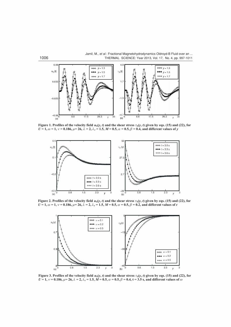
Figures 1 are sketched to show the velocity uS(y, t) and the shear stress tS(y, t) profiles

at different values of y. From these figures, it can be seen that the amplitude of the fluid oscilla-

tion decays away from the plate and approaches to zero. Figures 2 and 3 are prepared to show the

effect of time t and frequency of oscillation w on velocity and shear stress profiles. It is clear that

the amplitude of fluid oscillations decreases when time or frequency of oscillation w increases.

However, it is noticeable that this result cannot be generalized for all time because it possesses

monotonic behavior. The effect of magnetic parameter M and kinematic viscosity n is shown in

figs. 4 and 5. The increasing values of these parameters also decrease the amplitude of fluid os-

cillation. However, the shear stress for both cases change its monotonicity away from the plate.

The influence of relaxation and retardation times l and lr is depicted in figs. 6 and 7. As ex-



Figure 1. Profiles of the velocity field uS(y, t) and the shear stress tS(y, t) given by eqs. (15) and (22), forU = 1, w = 1, n = 0.186, m= 26, l = 2, lr = 1.5, M = 0.5, a = 0.5, b = 0.4, and different values of y

Figure 2. Profiles of the velocity field uS(y, t) and the shear stress tS(y, t) given by eqs. (15) and (22), forU = 1, w = 1, n = 0.186, m= 26, l = 2, lr = 1.5, M = 0.5, a = 0.5, b = 0.2, and different values of t

Figure 3. Profiles of the velocity field uS(y, t) and the shear stress tS(y, t) given by eqs. (15) and (22), forU = 1, n = 0.186, m= 26, l = 2, lr = 1.5, M = 0.5, a = 0.5, b = 0.4, t = 3.5 s, and different values of w


Figure 4. Profiles of the velocity field uS(y, t) and the shear stress tS(y, t) given by eqs. (15) and (22), forU = 1, w = 1, n = 0.186, m= 26, l = 2, lr = 1.5, a = 0.5, b = 0.4, t = 3.5 s, and different values of M

Figure 5. Profiles of the velocity field uS(y, t) and the shear stress tS(y, t) given by eqs. (15) and (22), forU = 1, w = 1, r= 140, l = 2, lr = 1.5, a = 0.5, b = 0.4, t = 3.5 s, and different values of n

Figure 6. Profiles of the velocity field uS(y, t) and the shear stress tS(y, t) given by eqs. (15) and (22), forU = 1, w = 1, n = 0.186, m= 26, lr = 0.1, M = 0.5, a = 0.3, b = 0.2, t = 3.5 s, and different values of l

pected their effects on fluid oscillations are opposite. For instance, it is easy to see that for large

values of y, the behavior of relaxation time is shear-thickening while retardation time has

shear-thinning behavior on fluid oscillations.

More important for us is to discuss the effects of fractional parameters a and b of the

model. In figs. 8 and 9, we depict the profiles of velocity uS(y, t) and shear stress uS(y, t) for three

different values of a and b. It is observed from these figures that a shows a shear-thinning be-

havior while b depicts a shear-thickening behavior. As b strengthens the shear-thickening, the

amplitude of fluid oscillation away from the plate is also reduced whilea depicts an opposite be-

havior. Finally, for comparison, the velocity field and the shear stress corresponding to the four

models (fractional Oldroyd-B, fractional Maxwell, fractional second grade and Newtonian) for

magnetic and without magnetic effect are together depicted in figs. 10 and 11. It is clearly seen

from these figures that fractional Maxwell fluids have largest and the fractional M0nd grade flu-

ids have the smallest amplitude of fluid oscillations for velocity field as well as shear stress,

whether magnetic effect is present or not. The units of the material parameters in all figures are

SI units.


Figure 7. Profiles of the velocity field uS(y, t) and the shear stress tS(y, t) given by eqs. (15) and (22), forU = 1, w = 1, n = 0.186, m= 26, l = 5, M = 0.5, a = 0.5, b = 0.4, t = 3.5 s, and different values of lr

Figure 8. Profiles of the velocity field uS(y, t) and the shear stress tS(y, t) given by eqs. (15) and (22), forU = 1, w = 1, n = 0.186, m= 26, l = 2, lr = 1.5, M = 0.5, b = 0.1, t = 3.5 s, and different values of a


Figure 9. Profiles of the velocity field uS(y, t) and the shear stress tS(y, t) given by eqs. (15) and (22), forU = 1, w = 1, n = 0.186, m= 26, l = 2, lr = 1.5, M = 0.5, a = 0.9, t = 3.5 s, and different values of b

Figure 10. Profiles of the velocity field uS(y, t) and the shear stress tS(y, t) for fractional MHD Oldroyd-B(l = 5, lr = 1.5), fractional MHD Maxwell (l = 5, lr = 1.5), fractional MHD second grade (l = 0, lr = 1,5), andMHD Newtonian (l= 0, lr = 0) fluids, for U = 1,w= 1, n= 0.186,m= 26, M = 0.5,a= 0.5, b= 0.4 ,and t = 3.5 s

Figure 11. Profiles of the velocity field uS(y, t) and the shear stress tS(y, t) for fractional MHD Oldroyd-B(l = 5, lr = 1.5), fractional MHD Maxwell (l = 5, lr = 0), fractional MHD second grade (l = 0, lr = 1.5), andMHD Newtonian (l= 0, lr = 0) fluids, for U = 1,w= 1, n= 0.186,m= 26, M = 0.5,a= 0.5, b= 0.4, and t = 3.5 s

Concluding remarks

The purpose of this paper is to establish exact solutions corresponding to oscillating

motion of a MHD Oldroyd-B fluid with fractional derivatives. Analytical expressions for veloc-

ity fields and the corresponding shear stresses for flows due to oscillations of an infinite flat

plate were determined using discrete Laplace transform for sequential fractional derivatives.

The solutions that have been obtained, presented in series form in terms of the Fox H-functions,

satisfy all imposed initial and boundary conditions. In special cases the solutions for ordinary

MHD Oldroyd-B , fractional and ordinary MHD Maxwell, fractional and ordinary MHD second

grade, and MHD Newtonian fluid as well as those for hydrodynamic fluids are obtained from

general solutions. Many previously known results are recovered from the present results, such

as Stokes' first and second problems for MHD and hydrodynamic Oldroyd-B, Maxwell, second

grade and Newtonian fluids. The results categorically indicate the following findings.

! The amplitude of the fluid oscillation decays away from the plate and approaches to zero.

! The amplitude of fluid oscillation decreases when time or frequency of oscillation w

increases, however this result cannot be generalized.

! The influence of magnetic field M and kinematic viscosity n decrease the amplitude of

oscillation.

! The relaxation time implies shear-thickening while the retardation time implies shear-thin-

ning behavior on the fluid motion.

! The fractional Maxwell fluid have the largest and fractional second grade have the smallest

amplitude of oscillations independent of the magnetic field.

References

[1] Fenton, R., The Transient for Stokes' Oscillating Plane: A Solution in Terms of Tabulated Functions, J.Fluid. Mech., 31 (1968), 1, pp. 810-825

[2] Puri, P., Kythe, P. K., Nonclassical Thermal Effects in Stokes' Second Problem, Acta Mech., 112 (1995),1-4, pp. 1-9

[3] Erdogan, M. E. , A Note on an Unsteady Flow of a Viscous Fluid Due to an Oscillating Plane Wall,Internat. J. Non-Linear Mech., 35 (2000), 1, pp. 281-285

[4] Rajagopal, K. R., Longitudinal and Torsional Oscillations of a Rod in a Non-Newtonian Fluid, Acta.Mech., 49 (1983), 3-4, pp. 281-285

[5] Rajagopal, K. R., Bhatnagar, R. K., Exact Solutions for Some Simple Flows of an Oldroyd-B Fluid, Acta.Mech., 113 (1995), 1-4, pp. 233-239

[6] Hayat, T., et al., Some Simple Flows of an Oldroyd-B Fluid, Int. J. Engrg. Sci., 39 (2001), 2, pp. 135-147[7] Aksel, N., et al., Starting Solutions for Some Unsteady Unidirectional Flows of Oldroyd-B Fluids, Z.

Angew. Math. Phys., 57 (2006), 5, pp. 815-831[8] Khan, M., et al., Hall Effect on the Pipe Flow of a Burgers' Fluid: An Exact Solution, Nonlinear Anal.:

Real World Appl., 10 (2009), 2, pp. 974-979[9] Fetecau, C., Fetecau Corina, Starting Solutions for Some Unsteady Unidirectional Flows of a Second

Grade Fluid, Int. J. Engrg. Sci., 43 (2005), 10, pp. 781-789[10] Fetecau, C., Fetecau Corina, Starting Solutions for the Motion of a Second Grade Fluid Due to Longitudi-

nal and Torsional Oscillations of a Circular Cylinder, Int. J. Engrg. Sci., 44 (2006), pp. 788-796[11] Khan, M., et al., On Exact Solutions for Some Oscillating Motions of a Generalized Oldroyd-B Fluid, Z.

Angew. Math. Phys., 61 (2010), 1, pp. 133-145[12] Khan, M., et al., Exact Solutions for Some Oscillating Motions of a Fractional Burgers' Fluid, Math.

Comput. Modelling, 51 (2010), 5-6, pp. 682-692[13] Mahmood, A., et al., Some Exact Solutions of the Oscillatory Motion of a Generalized Second Grade Fluid

in an Annular Region of Two Cylinders, Acta Mech Sin, 26 (2010), 4, pp. 541-550[14] Zheng, L., et al., Exact Solutions for Generalized Maxwell Fluid Flow Due to Oscillatory and Constantly

Accelerating Plate, Nonlinear Anal.: Real World Appl., 11 (2010), 5, pp. 3744-3751[15] Anjum, A., et al., Starting Solutions for Oscillating Motions of an Oldroyd-B Fluid over a Plane Wall,

Commun Nonlinear Sci Numer Simulat, 17 (2012), 1, pp. 472-482


[16] Bagley, R. L., A Theoretical Basis for the Application of Fractional Calculus to Viscoelasticity, J. Rheol.,27 (1983), 1, pp. 201-210

[17] Heibig, A., Palade, L. I., On the Rest State Stability of an Objective Fractional Derivative ViscoelasticFluid Model, J. Math. Phys., 49 (2008), 1, pp. 43-101

[18] Song, D. Y., Study of Rheological Characterization of Fenu-Greek Gum with Modified Maxwell, J. Chem.Eng., 8 (2008), 1, pp. 85-88

[19] Wang, S., Xu, M., Axial Coutte Flow of Two Kinds of Fractional Viscoelastic Fluids in an Annulus, Non-linear Anal: Real World Appl. 10 (2009), 2, pp. 1087-1096

[20] Fetecau, C., et al., Exact Solutions for the Flow of a Viscoelastic Fluid Induced by a Circular CylinderSubject to a Time Dependent Shear Stress, Commun Nonlinear Sci Numer Simulat, 15 (2010), 12, pp.3931-3938

[21] Tripathi, D., et al., Peristaltic Flow of Viscoelastic Fluid with Fractional Maxwell Model through a Chan-nel, Applied Mathematics and Computation, 215 (2010), pp. 3645-3654

[22] Hyat, T., et al., On Exact Solutions for Oscillatory Flows in a Generalized Burgers' Fluid with Slip Condi-tion, Z. Naturforsch, 65a (2010), 10, pp. 381-391

[23] Hayat, T., et al., Flows in a Fractional Generalized Burgers' Fluid, J. Porus Media, 13 (2010), 8, pp.725-739

[24] Tripathi, D., Peristaltic Flow of a Fractional Second Grade Fluid through a Cylindrical Tube, Thermal Sci-ence 15 (2011), Suppl. 2, pp. S167-S173

[25] Liu, Y., Zheng, L., Unsteady MHD Couette Flow of a Generalized Oldroyd-B Fluid with Fractional De-rivative, Comput. Math. Appl., 61 (2011), 2, pp. 443-450

[26] Zheng, L., et al., Slip Effects on MHD Flow of a Generalized Oldroyd-B Fluid with Fractional Derivative,Nonlinear. Anal.: Real World Appl., 13 (2012), 2, pp. 513-523

[27] Fetecau, C., et al., Flow of Fractional Maxwell Fluid between Coaxial Cylinders, Arch. App. Mech., 81(2011), 1, pp. 1153-1163

[28] Jamil, M., et al., New Exact Analytical Solutions for Stokes' First Problem of Maxwell Fluid with Frac-tional Derivative Approach, Comput. Math. Appl., 62 (2011), 3, pp. 1013-1023

[29] Jamil, M., et al., Translational Flows of an Oldroyd-B Fluid with Fractional Derivatives, Comput. Math.Appl., 62 (2011), 3, pp. 1540-1553

[30] Siddique, I., Vieru, D., Exact Solutions for Rotational Flow of a Fractional Maxwell Fluid in a CircularCylinder, Thermal Science, 16 (2011), 2, pp. 345-355

[31] Tripathi, D., et al., Influence of Slip Condition on Peristaltic Tansport of a Viscoelastic Fluid with Model,Thermal Science, 15 (2011), 2, pp. 501-515

[32] Tripathi, D., Peristaltic Transport of Fractional Maxwell Fluids in Uniform Tubes: Application of an En-doscope, Computers and Mathematics with Applications, 62 (2011), 3, pp. 1116-1126

[33] Tripathi, D., Peristaltic Transport of a Viscoelastic Fluid in a Channel, Acta Astronautica, 68 (2011), 7, pp.1379-1385

[34] Tripathi, D., et al., Peristaltic Transport of a Generalized Burgers' Fluid: Application to the Movement ofChyme in Small Intestine, Acta Astronautica, 69 (2011), 1, pp. 30-38

[35] Tripathi, D., Numerical Study on Peristaltic Flow of Generalized Burgers' Fluids in Uniform Tubes inPresence of an Endoscope, International Journal for Numerical Methods in Biomedical Engineering, 27(2011), 11, pp. 1812-1828

[36] Beg, O. A., et al., Numerical Study of Magnetohydrodynamic Viscous Plasma Flow in Rotating PorousMedia with Hall Currents and Inclined Magnetic Field Influence, Communications in Nonlinear Scienceand Numerical Simulation, 15 (2010), 2, pp. 345-359

[37] Pandey, S. K., Tripathi, D., Influence of Magnetic Field on the Peristaltic Flow of a Viscous Fluidthrough a Finite-Length Cylindrical Tube, Applied Bionics and Biomechanics, 7 (2010), 3, pp. 169-176

[38] Pandey, S. K., Tripathi, D., Peristaltic Flow Characteristics of Maxwell and Magneto-HydrodynamicFluids in Finite Channels, Journal of Biological Systems, 18 (2010), 3, pp. 621-647

[39] Podlubny, I., Fractional Differential Equations, Academic press, San Diego, Cal., USA, 1999[40] Mainardi, F., Fractional Calculus and Waves in Viscoelasticity: An Introduction to Mathematical Models,

Imperial College Press, London, 2010[41] Mathai, A. M., et al., The H-Functions: Theory and Applications, Springer, New York, USA, 2010[42] Debnath, L., Bhatta, D., Integral Transforms and Their Applications, 2nd ed., Chapman & Hall/CRC,

Boca Raton, Fla., USA, 2007

Paper submitted: July 31, 2011Paper revised: October 22, 2011Paper accepted: October 26, 2011


FRACTIONAL MAGNETOHYDRODYNAMICS …...FRACTIONAL MAGNETOHYDRODYNAMICS OLDROYD-B FLUID OVER AN...

Documents

Transcript of FRACTIONAL MAGNETOHYDRODYNAMICS …...FRACTIONAL MAGNETOHYDRODYNAMICS OLDROYD-B FLUID OVER AN...