Fractional Graph Theory - Department of Applied ... · PDF file6.1 Relaxing isomorphism 93 6.2...
167
Fractional Graph Theory A Rational Approach to the Theory of Graphs Edward R. Scheinerman The Johns Hopkins University Baltimore, Maryland Daniel H. Ullman The George Washington University Washington, DC With a Foreword by Claude Berge Centre National de la Recherche Scientifique Paris, France
Transcript of Fractional Graph Theory - Department of Applied ... · PDF file6.1 Relaxing isomorphism 93 6.2...

Fractional Graph TheoryA Rational Approach to the Theory of Graphs
Edward R. ScheinermanThe Johns Hopkins UniversityBaltimore, Maryland
Daniel H. UllmanThe George Washington UniversityWashington, DC
With a Foreword by
Claude BergeCentre National de la Recherche ScientifiqueParis, France

c©2008 by Edward R. Scheinerman and Daniel H. Ullman.This book was originally published by John Wiley & Sons. The copyright has reverted to theauthors.Permission is hereby granted for readers to download, print, and copy this book for free so long asthis copyright notice is retained. The PDF file for this book can be found here:
http://www.ams.jhu.edu/~ers/fgt

To Rachel, Sandy, Danny, Jessica, Naomi, Jonah, and Bobby

Contents
Foreword vii
Preface viii
1 General Theory: Hypergraphs 1
1.1 Hypergraph covering and packing 11.2 Fractional covering and packing 21.3 Some consequences 41.4 A game-theoretic approach 51.5 Duality and duality 61.6 Asymptotic covering and packing 71.7 Exercises 121.8 Notes 13
2 Fractional Matching 14
2.1 Introduction 142.2 Results on maximum fractional matchings 172.3 Fractionally Hamiltonian graphs 212.4 Computational complexity 262.5 Exercises 272.6 Notes 28
3 Fractional Coloring 30
3.1 Definitions 303.2 Homomorphisms and the Kneser graphs 313.3 The duality gap 343.4 Graph products 383.5 The asymptotic chromatic and clique numbers 413.6 The fractional chromatic number of the plane 433.7 The Erdos-Faber-Lovasz conjecture 493.8 List coloring 513.9 Computational complexity 533.10 Exercises 543.11 Notes 56
iv

Contents v
4 Fractional Edge Coloring 57
4.1 Introduction 574.2 An exact formula 584.3 The matching polytope 594.4 Proof and consequences 614.5 Computational complexity 634.6 Fractional total chromatic number 634.7 Exercises 704.8 Notes 71
5 Fractional Arboricity and Matroid Methods 72
5.1 Arboricity and maximum average degree 725.2 Matroid theoretic tools 735.3 Matroid partitioning 775.4 Arboricity again 815.5 Maximum average degree again 845.6 Duality, duality, duality, and edge toughness 855.7 Exercises 905.8 Notes 91
6 Fractional Isomorphism 93
6.1 Relaxing isomorphism 936.2 Linear algebra tools 966.3 Equitable partitions 1006.4 Iterated degree sequences 1016.5 The main theorem 1026.6 Other relaxations of isomorphism 1056.7 Exercises 1086.8 Notes 110
7 Fractional Odds and Ends 111
7.1 Fractional topological graph theory 1117.2 Fractional cycle double covers 1137.3 Fractional Ramsey theory 1147.4 Fractional domination 1167.5 Fractional intersection number 1217.6 Fractional dimension of a poset 1257.7 Sperner’s theorem: a fractional perspective 1277.8 Exercises 1287.9 Notes 129

vi Contents
A Background 131
A.1 Basic graph theory and notation 131A.2 Hypergraphs, multigraphs, multisets, fuzzy sets 134A.3 Linear programming 134A.4 The subadditivity lemma 137A.5 Exercises 138A.6 Notes 138
Bibliography 139
Author Index 148
Subject Index 152
Foreword
Graph theory is one of the branches of modern mathematics having experienced a most impressivedevelopment in recent years. In the beginning, Graph Theory was only a collection of recreationalor challenging problems like Euler tours or the four coloring of a map, with no clear connectionamong them, or among techniques used to attach them. The aim was to get a “yes” or “no” answerto simple existence questions. Under the impulse of Game Theory, Management Sciences, andTransportation Network Theory, the main concern shifted to the maximum size of entities attachedto a graph. For instance, instead of establishing the existence of a 1-factor, as did Petersen andalso Konig (whose famous theorem on bipartite graphs was discovered 20 years earlier by Steinitzin his dissertation in Breslau), the main problem was now to study the maximum number ofedges in a matching, even if not a 1-factor or “perfect matching”. In this book, Scheinerman andUllman present the next step of this evolution: Fractional Graph Theory. Fractional matchings,for instance, belong to this new facet of an old subject, a facet full of elegant results.
By developing the fractional idea, the purpose of the authors is multiple: first, to enlarge thescope of applications in Scheduling, in Operations Research, or in various kinds of assignmentproblems; second, to simplify. The fractional version of a theorem is frequently easier to prove thanthe classical one, and a bound for a “fractional” coefficient of the graph is also a bound for theclassical coefficient (or suggests a conjecture). A striking example is the simple and famous theoremof Vizing about the edge-chromatic number of a graph; no similar result is known for the edge-chromatic number of a hypergraph, but the reader will find in this book an analogous statement forthe “fractional” edge-chromatic number which is a theorem. The conjecture of Vizing and Behzadabout the total chromatic number becomes in its fractional version an elegant theorem.
This book will draw the attention of the combinatorialists to a wealth of new problems andconjectures. The presentation is made accessible to students, who could find a clear expositionof the background material and a stimulating collection of exercises. And, above all, the pleasureafforded by these pages will contribute to making Combinatorics more appealing to many.
Claude BergeParis, France
vii

Preface
Graphs model a wide variety of natural phenomena, and it is the study of these phenomena thatgives rise to many of the questions asked by pure graph theorists. For example, one motivationfor the study of the chromatic number in graph theory is the well-known connection to schedulingproblems. Suppose that an assortment of committees needs to be scheduled, each for a total of onehour. Certain pairs of committees, because they have a member in common, cannot meet at thesame time. What is the length of the shortest time interval in which all the committees can bescheduled?
Let G be the graph whose vertices are these committees, with an edge between two committeesif they cannot meet at the same time. The standard answer to the scheduling question is that thelength of the shortest time interval is the chromatic number of G. As an illustration, suppose thatthere are 5 committees, with scheduling conflicts given by the graph in Figure A. Since G can be
1
2
34
5
Figure A: The graph C5, colored with three colors.
colored with 3 colors, the scheduling can be done in 3 hours, as is illustrated in Figure B.It is a widely held misconception that, since the chromatic number of G is 3, the schedule in
Figure B cannot be improved. In fact, the 5 committees can be scheduled in two-and-a-half hours,as is illustrated in Figure C.
All that is required is a willingness to allow one committee to meet for half an hour, to interrupttheir meeting for a time, and later to reconvene for the remaining half hour. All that is requiredis a willingness to break one whole hour into fractions of an hour—to break a discrete unit intofractional parts. The minimum length of time needed to schedule committees when interruptionsare permitted is not the chromatic number of G but the less well-known fractional chromatic numberof G.
This example illustrates the theme of this book, which is to uncover the rational side of graphtheory: How can integer-valued graph theory concepts be modified so they take on nonintegralvalues? This “fractionalization” bug has infected other parts of mathematics. Perhaps the best-known example is the fractionalization of the factorial function to give the gamma function. Fractalgeometry recognizes objects whose dimension is not a whole number [126]. And analysts considerfractional derivatives [132]. Some even think about fractional partial derivatives!
We are not the first to coin the term fractional graph theory; indeed, this is not the first book
viii

Preface ix
1 2 3 4 512:00
1:00
2:00
3:00
Figure B: A schedule for the five committees.
1 2 3 4 512:00
1:00
2:00
3:00
Figure C: An improved schedule for the five committees.
on this subject. In the course of writing this book we found that Claude Berge wrote a shortmonograph [16] on this very subject. Berge’s Fractional Graph Theory is based on his lecturesdelivered at the Indian Statistical Institute twenty years ago. Berge includes a treatment of thefractional matching number and the fractional edge chromatic number.1 Two decades have seena great deal of development in the field of fractional graph theory and the time is ripe for a newoverview.
Rationalization
We have two principal methods to convert graph concepts from integer to fractional. The firstis to formulate the concepts as integer programs and then to consider the linear programmingrelaxation (see §A.3). The second is to make use of the subadditivity lemma (Lemma A.4.1 onpage 137). It is very pleasing that these two approaches typically yield the same results. Nearlyevery integer-valued invariant encountered in a first course in graph theory gives rise to a fractionalanalogue.
Most of the fractional definitions in this book can be obtained from their integer-valued coun-terparts by replacing the notion of a set with the more generous notion of a “fuzzy” set [190]. Whilemembership in a set is governed by a {0, 1}-valued indicator function, membership in a fuzzy set isgoverned by a [0, 1]-valued indicator function. It is possible to devise fractional analogues to nearly
1More recently, Berge devotes a chapter of his monograph Hypergraphs: Combinatorics of Finite Sets [19] tofractional transversals of hypergraphs, which includes an exploration of fractional matchings of graphs.

x Preface
any integer-valued graph-theoretic concept by phrasing the integer-valued definition in the rightway and then inserting the word “fuzzy” in front of the word “set” in the appropriate place. Al-though this lends a unifying spirit to the book, we choose to avoid this language in favor of spellingout the definitions of fractional invariants directly in terms of [0, 1]-valued labelings or functions.Nonetheless, the word “fractional” is meant to suggest the continuous unit interval [0, 1] in placeof the “discrete unit interval” {0, 1}. Further, “fractional” underscores the fact that the resultingreal numbers are almost always rational values in [0, 1].
Goals
The focus of this book is not on the theory of mathematical programming, although this theoryis used and certain polytopes of interest to the programming theorist do make appearances here.Neither is the focus on algorithms and complexity, although these issues are discussed in places.Rather, the main goal is to prove theorems that are analogous to the main theorems of basic graphtheory. For example, one might ask if there is a fractional analogue of the four-color theorem. Onemight hope to prove a fractional three-and-a-half-color result saying that the fractional chromaticnumber of any planar graph is no more than 7/2 (in fact, this is obviously false) or one mighthope to prove a fractional four-and-a-half-color result via an argument that does not rely on thefour-color theorem itself (no such proof is known). The focus is on comparing and contrastinga fractional graph invariant to its integer-valued cousin and on discerning to what degree basicproperties and theorems of the integer-valued invariant are retained by the fractional analogue.
Our goal has been to collect in one place the results about fractional graph invariants that onecan find scattered throughout the literature and to give a unified treatment of these results. Wehave highlighted the theorems that seem to us to be attractive, without trying to be encyclopedic.There are open questions and unexplored areas here to attract the active researcher. At the sametime, this book could be used as a text for a topics course in graph theory. Exercises are includedin every chapter, and the text is meant to be approachable for graduate students in graph theoryor combinatorial optimization.
Chapter Overview
In Chapter 1 we develop a general fractional theory of hypergraphs to which we regularly referin the subsequent chapters. In Chapters 2, 3, and 4 we study the fractional analogues of thematching number, the chromatic number, and the edge chromatic number. In Chapter 5 we studyfractional arboricity via matroids. In Chapter 6 we discuss an equivalence relation on graphs thatweakens isomorphism and is called fractional isomorphism. In Chapter 7 we touch on a number ofother fractional notions. Finally, the Appendix contains background material on notation, graphs,hypergraphs, linear programming, and the subadditivity lemma.
Each chapter features exercises and a Notes section that provides references for and furtherinformation on the material presented.
Acknowledgments
We would like to give thanks to a number of people who have assisted us with this project.Thanks to Dave Fisher, Leslie Hall, Mokutari Ramana, and Jim Propp, for inspiring conversa-
tions.Thanks to Noga Alon, Brian Alspach, Arthur Hobbs, Luis Goddyn, and Saul Stahl for a number
of helpful suggestions and ideas for material.

Preface xi
Thanks to Donniell Fishkind, Bilal Khan, Gregory Levin, Karen Singer, Brenton Squires, andYi Du (JHU), and to Phyllis Cook, Eric Harder, Dave Hough, Michael Matsko, and Elie Tannous(GWU), graduate students who read early drafts of the manuscript and offered numerous helpfulsuggestions.
Thanks to Claude Berge for writing the Foreword.Thanks to Andy Ross for the wonderful cover design.Thanks also to Jessica Downey and Steven Quigley, our editors at Wiley, for their enthusiasm
for and support of this project. We also acknowledge and appreciate the comments and suggestionsof the anonymous reviewers.
And finally, thanks to our wives, Amy and Rachel, who endure our obsessions with patienceand good humor.
Feedback
We appreciate your comments and reactions. Feel free to reach us by e-mail at [email protected](Scheinerman) or [email protected] (Ullman).
Finally
It is possible to go to a graph theory conference and to ask oneself, at the end of every talk,What is the fractional analogue? What is the right definition? Does the fractional version of thetheorem still hold? If so, is there an easier proof and can a stronger conclusion be obtained? Ifthe theorem fails, can one get a proof in the fractional world assuming a stronger hypothesis? Wecan personally attest that this can be an entertaining pastime. If, after reading this book, youtoo catch the fractional bug and begin to ask these questions at conferences, then we will considerourselves a success. Enjoy!
—ES, Baltimore—DU, Washington, D.C.
Exercise
1. Let f : R→ R by f(x) = x. The half derivative of f is 2√x/π. Why?
1
General Theory: Hypergraphs
Our purpose is to reveal the rational side of graph theory: We seek to convert integer-baseddefinitions and invariants into their fractional analogues. When we do this, we want to be sure thatwe have formulated the “right” definitions—conversions from integer to real that are, in some sense,natural. Here are two ways we might judge if an integer-to-real conversion process is natural: First,when two seemingly disparate conversions yield the same concept, then we feel confident that thefractionalized concept is important (and not tied to how we made the conversion). Second, when thesame conversion process works for a variety of concepts (e.g., we convert from matching number andchromatic number to their fractional analogues by the same methods), then we feel we have arrivedat a reasonable way to do the integer-to-real transformation. Happily, we can often satisfy both ofthese tests for “naturalness”. If a variety of attractive theorems arise from the new definition, thenwe can be certain that we are on the right track.
This chapter develops two general methods for fractionalizing graph invariants: linear relaxationof integer programs and applications of the subadditivity lemma.1 We present both methods andprove that they yield the same results.
1.1 Hypergraph covering and packing
A hypergraph H is a pair (S,X ), where S is a finite set and X is a family of subsets of S. The setS is called the ground set or the vertex set of the hypergraph, and so we sometimes write V (H) forS. The elements of X are called hyperedges or sometimes just edges.
A covering (alternatively, an edge covering) of H is a collection of hyperedges X1,X2, . . . ,Xj
so that S ⊆ X1 ∪ · · · ∪Xj . The least j for which this is possible (the smallest size of a covering) iscalled the covering number (or the edge covering number) of H and is denoted k(H).
An element s ∈ S is called exposed if it is in no hyperedges. If H has an exposed vertex, then nocovering of H exists and k(H) = ∞. Hypergraphs are sometimes known as set systems, althoughin that case one often forbids exposed vertices.
The covering problem can be formulated as an integer program (IP). To each set Xi ∈ Xassociate a 0,1-variable xi. The vector x is an indicator of the sets we have selected for the cover.Let M be the vertex-hyperedge incidence matrix of H, i.e., the 0,1-matrix whose rows are indexedby S, whose columns are indexed by X , and whose i, j-entry is 1 exactly when si ∈ Xj . Thecondition that the indicator vector x corresponds to a covering is simply Mx ≥ 1 (that is, everycoordinate of Mx is at least 1). Thus k(H) is the value of the integer program “minimize 1txsubject to Mx ≥ 1” where 1 represents a vector of all ones. Further, the variables in this andsubsequent linear programs are tacitly assumed to be nonnegative.
1These central ideas (linear programming and subadditivity), as well as other basic material, are discussed inAppendix A. The reader is encouraged to peruse that material before proceeding.
1

2 Chapter 1. General Theory: Hypergraphs
The covering problem has a natural dual. Let H = (S,X ) be a hypergraph as before. A packing(a vertex packing) in H is a subset Y ⊆ S with the property that no two elements of Y are togetherin the same member of X . The packing number p(H) is defined to be the largest size of a packing.The packing number of a graph is its independence number α.
Note that ∅ is a packing, so p(H) is well defined.There is a corresponding IP formulation. Let yi be a 0,1-indicator variable that is 1 just when
si ∈ Y . The condition that Y is a packing is simply M ty ≤ 1 where M is, as above, the vertex-hyperedge incidence matrix of H. Thus p(H) is the value of the integer program “maximize 1tysubject to M ty ≤ 1.” This is the dual IP to the covering problem and we have therefore provedthe following result.
Proposition 1.1.1 For a hypergraph H, we have p(H) ≤ k(H). �
Many graph theory concepts can be seen as hypergraph covering or packing problems. Forinstance, the chromatic number χ(G) is simply k(H) where the hypergraph H = (S,X ) has S =V (G) and X is the set of all independent subsets of V (G). Similarly, the matching number μ(G) isp(H) where H = (S,X ) has S = E(G) and X contains those sets of edges of G incident on a fixedvertex.
1.2 Fractional covering and packing
There are two ways for us to define the fractional covering and packing numbers of a hypergraphH. The first is straightforward. Since k(H) and p(H) are values of integer programs, we define thefractional covering number and fractional packing number of H, denoted k∗(H) and p∗(H) respec-tively, to be the values of the dual linear programs “minimize 1tx s.t. Mx ≥ 1” and “maximize1ty s.t. M ty ≤ 1”. By duality (Theorem A.3.1 on page 135) we have k∗(H) = p∗(H).
(Note that if H has an exposed vertex then the covering LP is infeasible and the packing LP isunbounded; let us adopt the natural convention that, in this case, we set both k∗ and p∗ equal to∞.)
We will not use the ∗ notation much more. There is a second way to define the fractionalcovering and packing numbers of H that is not a priori the same as k∗ and p∗; the ∗ notation istemporary until we show they are the same as kf and pf defined below.
We begin by defining t-fold coverings and the t-fold covering number of H. Let H = (S,X ) bea hypergraph and let t be a positive integer. A t-fold covering of H is a multiset {X1,X2, . . . ,Xj}(where each Xi ∈ X ) with the property that each s ∈ S is in at least t of the Xi’s. The smallestcardinality (least j) of such a multiset is called the t-fold covering number of H and is denotedkt(H). Observe that k1(H) = k(H).
Notice that kt is subadditive in its subscript, that is,
ks+t(H) ≤ ks(H) + kt(H)
since we can form a (perhaps not smallest) (s+ t)-fold covering of H by combining a smallest s-foldcovering and a smallest t-fold covering. By the lemma of Fekete (Lemma A.4.1 on page 137) wemay therefore define the fractional covering number of H to be
kf (H) = limt→∞
kt(H)t
= inft
kt(H)t
.
Yes, we have called both k∗ and kf the fractional covering numbers—the punch line, of course, isthat these two definitions yield the same result. However, it is clear that k∗(H) must be a rational

1.2 Fractional covering and packing 3
number since it is the value of a linear program with integer coefficients; it is not clear that kf
is necessarily rational—all we know so far is that the limit kt(H)/t exists. We also know thatkt(H) ≤ tk1(H) = tk(H) and therefore kf (H) ≤ k(H).
In a similar way, we define a t-fold packing of H = (S,X ) to be a multiset Y (defined over thevertex set S) with the property that for every X ∈ X we have
∑s∈X
m(s) ≤ t
where m is the multiplicity of s ∈ S in Y . The t-fold packing number of H, denoted pt(H), is thesmallest cardinality of a t-fold packing. Observe that p1(H) = p(H).
Notice that pt is superadditive in its subscript, i.e.,
ps+t(H) ≥ ps(H) + pt(H).
This holds because we can form a (not necessarily largest) (s+t)-fold packing by combining optimals- and t-fold packings. Using an analogue of the subadditivity lemma (exercise 1 on page 138), wedefine the fractional packing number of H to be
pf (H) = limt→∞
pt(H)t
.
Note that since pt(H) ≥ tp1(H) = tp(H) we have that pf (H) ≥ p(H).
Theorem 1.2.1 The two notions of fractional covering and the two notions of fractional packingare all the same, i.e., for any hypergraph H we have
k∗(H) = kf (H) = p∗(H) = pf (H).
Proof. If H has an exposed vertex, then all four invariants are infinite. So we restrict to the casethat H has no exposed vertices.
We know that kf = pf by LP duality. We show the equality k∗ = kf ; the proof that p∗ = pf issimilar and is relegated to exercise 1 on page 12.
First we prove that k∗ ≤ kf . Let a be a positive integer. Let {X1, . . . ,Xj} be a smallest a-foldcovering of H and let xi be the number of times Xi appears in this covering. Then Mx ≥ a, andtherefore M(x/a) ≥ 1. Thus x/a is a feasible vector for the covering problem, hence k∗(H) ≤1t(x/a) = ka(H)/a. Since this holds for all positive integers a, we have k∗(H) ≤ kf (H).
Next we prove that k∗ ≥ kf . Let x be a vector that yields the value of the LP “minimize1t · x s.t. Mx ≥ 1”. We may assume that x is rational (since the data in the LP are all integers).Let n be the least common multiple of all the denominators appearing in the vector x; thus theentries in nx are all integers. Further, we have Mnx ≥ n. We can form an n-fold cover of H bychoosing hyperedge Xi with multiplicity nxi. The size of this n-fold cover is
∑i nxi = 1t ·nx. Thus,
nk∗(H) = 1t · nx ≥ kn(H). Furthermore, for any positive integer a, we also have (an)k∗(H) ≥kan(H). Since k∗(H) ≥ kan(H)/(an) for all a, we have k∗(H) ≥ kf (H). �

4 Chapter 1. General Theory: Hypergraphs
1.3 Some consequences
Since the fractional covering/packing number of H is the value of a linear program with integercoefficients, we have the following.
Corollary 1.3.1 If H has no exposed vertices, then kf (H) is a rational number. �
Not only is kf (H) rational, but we can choose the optimal weights xi of the Xi to be rationalnumbers as well. Let N be a common multiple of the denominators of the xi’s and consider kN (H).One checks that we can form an N -fold covering of H if we choose Xi with multiplicity Nxi;moreover, this is best possible since (
∑Nxi)/N =
∑xi = kf (H).
Corollary 1.3.2 If H has no exposed vertices, then there exists a positive integer s for whichkf (H) = ks(H)/s. �
Thus we know not only that lim kt(H)/t = inf kt(H)/t (Lemma A.4.1 on page 137) but alsothat both equal min kt(H)/t and this minimum is achieved for infinitely many values of t. We usethis fact next to obtain a strengthening of the subadditivity of ks(H).
Proposition 1.3.3 If H is any hypergraph, then there exist positive integers s and N such that,for all t ≥ N , ks(H) + kt(H) = ks+t(H).
Proof. Let s be as in the previous corollary so that kf (H) = ks(H)/s. Then, for any n ≥ 1,
kf (H) ≤ kns(H)/(ns) ≤ ks(H)/s = kf (H),
where the second inequality follows from the subadditivity of ks. Hence kns(H) = nks(H). Nowfix j with 0 ≤ j < s and for any positive integer n let an = kns+j(H) − kns(H). Clearly an is anonnegative integer. Also,
an+1 = k(n+1)s+j(H)− k(n+1)s(H)
= k(n+1)s+j(H)− (n+ 1)ks(H)
≤ kns+j(H) + ks(H)− (n+ 1)ks(H)
= kns+j(H)− nks(H)
= an,
where again the inequality follows from subadditivity. A nonincreasing sequence of positive integersis eventually constant; we thus have an integer Mj such that, if m,n ≥Mj, then am = an.
Let M = max{M0,M1, . . . ,Ms−1}. Then, whenever m,n ≥M , we have
kms+j(H)− kms(H) = kns+j(H)− kns(H)
for all j with 1 ≤ j < s. In particular, with m = n+ 1, we have
k(n+1)s+j(H) = kns+j(H) + ks(H)
for 1 ≤ j < s. Now let N = Ms. If t ≥ N , then put n = �t/s� and put j = t− sn. Then t = sn+ jwith n ≥M and 0 ≤ j < s, so
ks+t(H) = k(n+1)s+j(H) = kns+j(H) + ks(H) = kt(H) + ks(H).
This completes the proof. �

1.4 A game-theoretic approach 5
In fact, the proof shows that any subadditive sequence a1, a2, . . . of nonnegative integers forwhich inf{an/n} equals as/s satisfies the same conclusion: as+t = as + at for sufficiently larget. This implies that the sequence of differences dn = an+1 − an is eventually periodic, sincedt+s = at+s+1 − at+s = at+1 + as − at − as = dt for sufficiently large t.
In the presence of sufficient symmetry, there is a simple formula for kf (H). An automorphismof a hypergraph H is a bijection π : V (H)→ V (H) with the property that X is a hyperedge of Hiff π(X) is a hyperedge as well. The set of all automorphisms of a hypergraph forms a group underthe operation of composition; this group is called the automorphism group of the hypergraph. Ahypergraph H is called vertex-transitive provided for every pair of vertices u, v ∈ V (H) there existsan automorphism of H with π(u) = v.
Proposition 1.3.4 Let H = (S,X ) be a vertex-transitive hypergraph and let e = max{|X| : X ∈X}. Then kf (H) = |S|/e.
Proof. If we assign each vertex of H weight 1/e, then we have a feasible fractional packing. Thuskf (H) = pf (H) ≥ |S|/e. Note that no larger uniform weighting of the vertices is feasible.
Let Γ denote the automorphism group of H. Let w:S → [0, 1] be an optimal fractional packingof H and let π ∈ Γ. Then w ◦ π also is an optimal fractional packing of H. Since any convexcombination of optimal fractional packings is also an optimal fractional packing,
w∗(v) :=1|Γ|
∑π∈Γ
w[π(v)]
is an optimal fractional packing which, because H is vertex-transitive, assigns the same weight toevery vertex of H. Thus w∗(v) = 1/e and the result follows. �
1.4 A game-theoretic approach
Consider the following game, which we call the hypergraph incidence game, played on a hypergraphH = (S,X ). There are two players both of whom know H. In private, the vertex player chooses anelement s of S. Also in private, the hyperedge player chooses an X in X . The players then revealtheir choices. If s ∈ X then the vertex player pays the hyperedge player $1; otherwise there is nopayoff. Assuming both players play optimally, what is the expected payoff to the hyperedge player?This is a classic, zero-sum matrix game whose matrix is M , the vertex-hyperedge incidence matrix.The optimal strategy for the players is typically a mixed strategy wherein the vertex player choosesan element si ∈ S with probability yi and the hyperedge player chooses Xj ∈ X with probabilityxj. The value of such a game is defined to be the expected payoff assuming both players adopttheir optimal strategies.
Theorem 1.4.1 For a hypergraph H the value of the hypergraph incidence game played on H is1/kf (H).
Proof. First note that if there is an element s ∈ S that is in no X ∈ X (an exposed vertex) thenby playing s the vertex player can always avoid paying the hyperedge player; the value is 0 = 1/∞as claimed. We therefore restrict ourselves to hypergraphs with no exposed vertices.
From game theory, we know that the value of this game v∗ is the largest number v so thatMx ≥ v for any probability vector x. Likewise, v∗ is the smallest number v so that M ty ≤ v forall probability vectors y. Our claim is that v∗ = 1/kf (H) = 1/pf (H).

6 Chapter 1. General Theory: Hypergraphs
Let v∗ be the value of the game and let probability vector x∗ be an optimal mixed strategy forthe hyperedge player. We therefore have that Mx∗ ≥ v∗. Letting x = x∗/v∗, we note that Mx ≥ 1so x is a feasible covering and therefore kf (H) ≤ 1tx = 1tx∗/v∗ = 1/v∗ (since x∗ is a probabilityvector).
Now let probability vector y∗ be an optimal mixed strategy for the vertex player. Then M ty∗ ≤v∗ and therefore y = y∗/v∗ is a feasible packing. We therefore have pf (H) ≥ 1ty = 1ty∗/v∗ = 1/v∗.Since kf = pf , the result follows. �
1.5 Duality and duality
The matching and covering problems are dual in the sense of linear/integer programming. IfH = (S,X ) is a hypergraph and M is its vertex-hyperedge incidence matrix, then the problems ofcomputing k(H) and p(H) are dual integer programs:
k(H) = min1tx s.t. Mx ≥ 1, and
p(H) = max 1ty s.t. M ty ≤ 1.
The problems of computing kf (H) and pf (H) are the dual linear programs obtained from these IPsby relaxing the condition that the variables be integers.
For example, let G be a graph and let H = (V,X ) where V = V (G) and X is the set of allindependent subsets of V (G). Now k(H) is the minimum number of independent sets that containall vertices, i.e., χ(G). Similarly, p(H) is the maximum number of vertices, no two of which aretogether in an independent set, i.e., the maximum number ω(G) of pairwise adjacent vertices. Thisis the sense in which the graph problems of computing the chromatic number and the size of thelargest clique are dual.
Let us introduce a second notion of duality: hypergraph duality. LetH = (S,X ) be a hypergraphand write
S = {s1, . . . , sn} and X = {X1, . . . ,Xm}.Then M (the vertex-hyperedge incidence matrix) is n × m with Mij = 1 if and only if si ∈ Xj .We define the dual hypergraph of H, denoted H∗, to be the hypergraph with vertex set X andhyperedge set S with
X = {x1, . . . , xm} and S = {S1, . . . , Sn}
and we put xj ∈ Si exactly when si ∈ Xj (in H). In matrix language, the vertex-hyperedgeincidence matrices of H and H∗ are transposes of one another.
We now consider the covering and packing problems in H∗. A covering of H∗ is the smallestnumber of Si’s that include all the xj’s. From the perspective of H, we seek the minimum numberof elements si that intersect all the Xj ’s. A subset of S that is incident with all hyperedges is calleda transversal of H and the smallest size of a transversal of H is called the transversal number of Hand is denoted τ(H). Thus,
τ(H) = k(H∗).
Next, consider p(H∗). The packing number of the dual of H is the largest number of xi’s withno two in a common Sj. In terms of H, we seek the maximum number of hyperedges Xi that are
1.6 Asymptotic covering and packing 7
Covering number, kmin # hyperedges to contain vertices
min 1tx s.t. Mx ≥ 1
Packing number, pmax # vertices, no two in a hyperedge
max 1tx s.t. Mtx ≤ 1
Transversal number, τmin # vertices to touch hyperedges
min 1tx s.t. Mtx ≥ 1
Matching number, μmax # pairwise disjoint hyperedges
max 1tx s.t. Mx ≤ 1
Mathematical programming duality
Hyp
ergr
aph
dual
ity
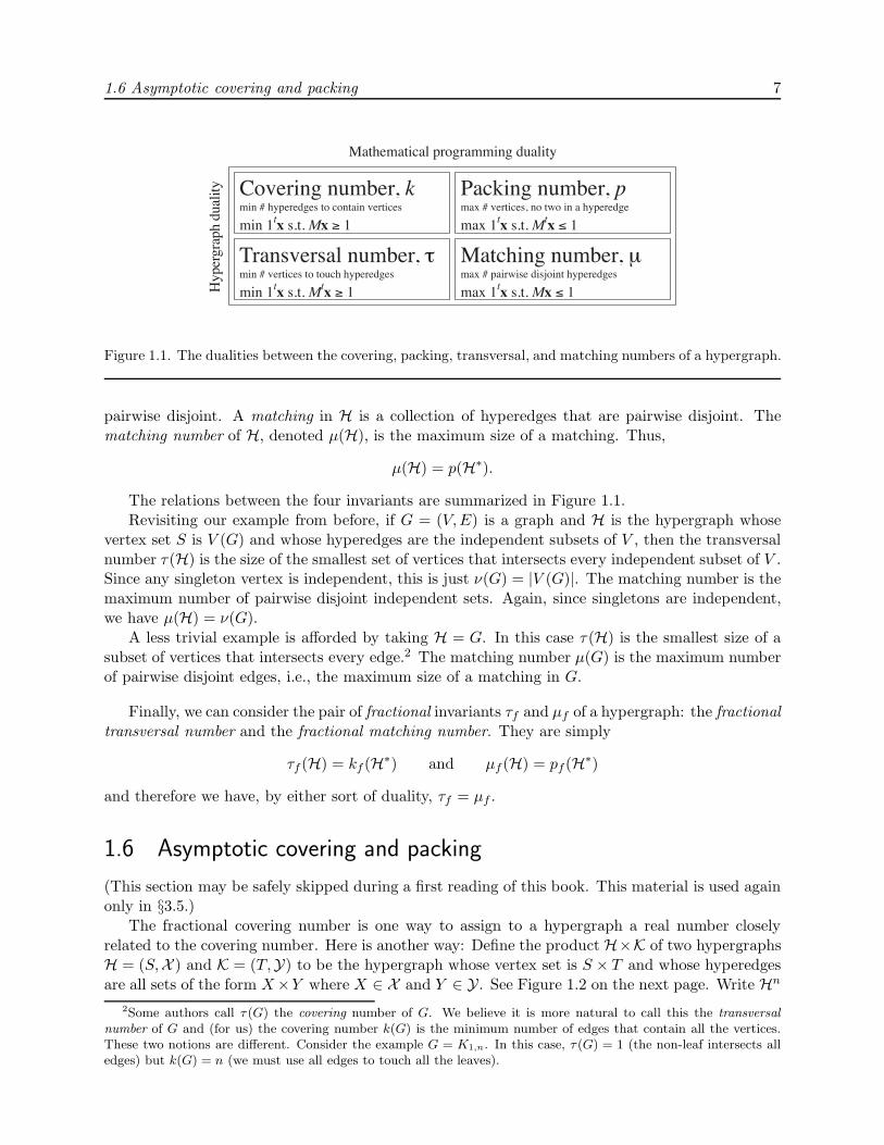
Figure 1.1. The dualities between the covering, packing, transversal, and matching numbers of a hypergraph.
pairwise disjoint. A matching in H is a collection of hyperedges that are pairwise disjoint. Thematching number of H, denoted μ(H), is the maximum size of a matching. Thus,
μ(H) = p(H∗).
The relations between the four invariants are summarized in Figure 1.1.Revisiting our example from before, if G = (V,E) is a graph and H is the hypergraph whose
vertex set S is V (G) and whose hyperedges are the independent subsets of V , then the transversalnumber τ(H) is the size of the smallest set of vertices that intersects every independent subset of V .Since any singleton vertex is independent, this is just ν(G) = |V (G)|. The matching number is themaximum number of pairwise disjoint independent sets. Again, since singletons are independent,we have μ(H) = ν(G).
A less trivial example is afforded by taking H = G. In this case τ(H) is the smallest size of asubset of vertices that intersects every edge.2 The matching number μ(G) is the maximum numberof pairwise disjoint edges, i.e., the maximum size of a matching in G.
Finally, we can consider the pair of fractional invariants τf and μf of a hypergraph: the fractionaltransversal number and the fractional matching number. They are simply
τf (H) = kf (H∗) and μf (H) = pf (H∗)
and therefore we have, by either sort of duality, τf = μf .
1.6 Asymptotic covering and packing
(This section may be safely skipped during a first reading of this book. This material is used againonly in §3.5.)
The fractional covering number is one way to assign to a hypergraph a real number closelyrelated to the covering number. Here is another way: Define the product H×K of two hypergraphsH = (S,X ) and K = (T,Y) to be the hypergraph whose vertex set is S × T and whose hyperedgesare all sets of the form X×Y where X ∈ X and Y ∈ Y. See Figure 1.2 on the next page. Write Hn
2Some authors call τ (G) the covering number of G. We believe it is more natural to call this the transversalnumber of G and (for us) the covering number k(G) is the minimum number of edges that contain all the vertices.These two notions are different. Consider the example G = K1,n. In this case, τ (G) = 1 (the non-leaf intersects alledges) but k(G) = n (we must use all edges to touch all the leaves).

8 Chapter 1. General Theory: Hypergraphs
Figure 1.2. An example of hypergraph product. The 20-vertex hypergraph is the product of the 4-vertexhypergraph (left) and the 5-vertex hypergraph (top). The vertex set of the product is the Cartesian productof the vertex sets of the factors. Hyperedges in the product are the Cartesian products of hyperedges of thefactors.
to be the nth power of H with respect to this product. We define the asymptotic covering numberto be
k∞(H) = infn
n
√k(Hn).
If A ⊆ X and B ⊆ Y are coverings of H and K respectively, then clearly the sets of the formsA×B, where A ∈ A and B ∈ B, form a covering of H×K. Hence k(H×K) ≤ k(H)k(K). Thus ifwe define g(n) to be log k(Hn), we see that g(m + n) ≤ g(m) + g(n). An appeal to Lemma A.4.1on page 137 then tells us that the infimum in the definition of k∞ is also a limit.
The dual invariant to the asymptotic covering number is naturally the asymptotic packingnumber, denoted p∞(H) and defined as supn
n√p(Hn). If A ⊆ S is a packing of H and B ⊆ T is a
packing of K, then A× B is a packing of H ×K. Using exercise 1 on page 138 and the argumentin the preceding paragraph, one sees that the supremum in this definition is also a limit.
We begin with the following result, which shows that the fractional covering number respectshypergraph products.
Theorem 1.6.1 If H and K are any hypergraphs, then
kf (H×K) = kf (H)kf (K) = pf (H)pf (K) = pf (H×K).
Proof. As above, write H = (S,X ) and K = (T,Y). If A is a smallest s-fold covering of H andB is a smallest t-fold covering of K, then the family of sets of the form A × B where A ∈ A andB ∈ B is an st-fold covering of H×K. Thus
kst(H×K)st
≤ ks(H)s· kt(K)
t

1.6 Asymptotic covering and packing 9
and it follows that kf (H×K) ≤ kf (H)kf (K).Similarly, if A ⊆ S is a largest s-fold packing of H and B ⊆ T is a largest t-fold packing of K,
then the set A×B is an st-fold packing of H×K. It follows that pf (H×K) ≥ pf (H)pf (K). Threeapplications of the duality theorem (via Theorem 1.2.1 on page 3) yield
kf (H×K) ≤ kf (H)kf (K) = pf (H)pf (K) ≤ pf (H×K) = kf (H×K),
and we are done. �
There is a curious lack of symmetry between the two asymptotic invariants. It may come asa surprise that the asymptotic covering number of a hypergraph is always equal to the fractionalcovering number of the hypergraph. Perhaps a greater surprise is that the same is not true of theasymptotic packing number. This is discussed in §3.5.Theorem 1.6.2 If H is any hypergraph, then k∞(H) = kf (H).
We provide two proofs: the first uses a random covering, and the second uses a greedy covering.We begin with a lemma.
Lemma 1.6.3 If H and K are any hypergraphs, then k(H×K) ≥ kf (H)k(K).
Proof. Suppose that H = (S,X ) and K = (T,Y). It is enough to show that there is a k(K)-foldcovering of H of cardinality k(H ×K). Let n = k(H×K). Consider a covering
{X1 × Y1,X2 × Y2, . . . ,Xn × Yn}of H×K. We claim that the multiset {X1,X2, . . . ,Xn} is the desired covering. Clearly it has theright cardinality. To see that it is a k(K)-fold covering, we must show that every s ∈ S is in Xi forat least k(K) of the indices i.
Fix s ∈ S. Let I ⊆ [n] be the set of indices i such that s ∈ Xi. We want to show that |I| ≥ k(K).Consider the multiset M = {Yi}i∈I . For every t ∈ T , we have (s, t) ∈ Xi×Yi for some i ∈ I. Hencet ∈ Yi. This shows that M is a covering of K and so I has cardinality at least k(K). �
Proof (of Theorem 1.6.2). Suppose that H = (S,X ). We first show that kf (H) ≤ k∞(H).Substituting Hn for K in Lemma 1.6.3 yields kf (H) ≤ k(Hn+1)/k(Hn). Since this is true for all n(including n = 0, if one understands H0 to be the hypergraph with one vertex and one nonemptyhyperedge),
kf (H) ≤ infn≥0
k(Hn+1)k(Hn)
≤ limn→∞
n
√k(H1)k(H0)
· k(H2)
k(H1)· · · k(H
n)k(Hn−1)
= limn→∞
n
√k(Hn)k(H0)
= k∞(H).
For the opposite inequality, suppose kf (H) = kt(H)/t and suppose K is a t-fold covering of H.Fix ε > 0. Pick a multiset M of hyperedges of Hn of cardinality
L =⌈(
kt(H)t
(1 + ε))n⌉

10 Chapter 1. General Theory: Hypergraphs
at random, each choice made independently and uniformly among the hyperedges of the form
E = X1 ×X2 × · · · ×Xn
where each Xi ∈ K. We show that for large enough n the probability that M = {E1, E2, . . . , EL}is a covering of Hn is positive, and, in fact, arbitrarily close to unity.
Let s = (s1, s2, . . . , sn) be an arbitrary element of the vertex set of Hn. A random hyperedgeE = X1×X2× · · · ×Xn contains s if and only if si ∈ Xi for all 1 ≤ i ≤ n. For each i, this happenswith probability at least t/kt(H) = 1/kf (H). Hence s ∈ E with probability at least (1/kf (H))n.Hence the probability that s is not in any of the hyperedges in M is less than
[1−
(1
kf (H)
)n]L
≤[1−
(1
kf (H)
)n](kf (H)(1+ε))n
=
[1−
(1
kf (H)
)n](kf (H))n(1+ε)n
.
Since limx→0 (1− x)1/x = 1e <
12 , the above probability is less than
(12
)(1+ε)n
for sufficiently large n. Since the cardinality of the vertex set of Hn is |S|n, the probability that Mis not a covering of Hn is less than
|S|n2(1+ε)n
.
The denominator grows superexponentially with n, but the numerator grows (merely) exponentiallywith n, so we can choose n so that this fraction is less than 1. For such an n, the probability thatM is a covering of Hn is positive, hence at least one such M exists. �
The following alternative proof of Theorem 1.6.2 produces a covering of Hn using a greedyapproach. The proof is quite short once we establish the following lemma.
Lemma 1.6.4 If H is any hypergraph and m is the maximum cardinality of a hyperedge in H, thenk(H) ≤ (1 + logm)kf (H).
Proof. Produce a covering of H in the following straightforward way. First pick a hyperedge X1 ofmaximal cardinality m. Inductively, pick Xi to be a hyperedge that contains the most elements ofthe vertex set not yet covered by X1,X2, . . . ,Xi−1. Continue picking hyperedges in this way untilevery element of the vertex set is in some Xi, and then stop.
The algorithm prescribes that |Xi − ∪i−1j=1Xj | is a nonincreasing function of i. Let ak denote
the number of indices i such that |Xi − ∪i−1j=1Xj | = k. Let a =
∑mk=1 ak. We show that a ≤
(1 + logm)kf (H). Since we have produced a covering of cardinality a, the optimal covering can beno larger, and the result follows.
In fact, we show that a ≤(1 + 1
2 + 13 + · · · + 1
m
)kf (H). To see this, for 1 ≤ j ≤ m let Hj be
the hypergraph whose ground set S is obtained from H by deleting all vertices covered by the firstam + am−1 + · · ·+ aj+1 hyperedges from the algorithm, and whose edge set is obtained from H byintersecting every hyperedge with the set S. (Take Hm to be H.) The hypergraph Hj has no edges

1.6 Asymptotic covering and packing 11
of cardinality greater than j, so no j-fold packing of Hj has fewer elements than the number ofelements of the vertex set of Hj, which is a1 + 2a2 + · · ·+ jaj . Hence, for 1 ≤ j ≤ m,
pj(H) ≥ pj(Hj) ≥ a1 + 2a2 + · · ·+ jaj .
Now kf (H) = pf (H) ≥ (pj(H)/j) for every j. It follows that, for 1 ≤ j ≤ m,
jkf (H) ≥ a1 + 2a2 + · · ·+ jaj . (∗)
For 1 ≤ j < m, divide equation (∗) by j(j + 1) and for j = m, divide inequality (∗) by m to obtain
12kf (H) ≥ 1
2a1
13kf (H) ≥ 1
2 · 3a1 +2
2 · 3a2
14kf (H) ≥ 1
3 · 4a1 +2
3 · 4a2 +3
3 · 4a3
...
1mkf (H) ≥ 1
(m− 1)ma1 +
2(m− 1)m
a2 + · · ·+ m− 1(m− 1)m
am−1
kf (H) ≥ 1ma1 +
2ma2 + · · ·+ m− 1
mam−1 +
m
mam.
Adding these inequalities yields(
12
+13
+14
+ · · ·+ 1m
+ 1)kf (H) ≥ a1 + a2 + a3 + · · ·+ am. (∗∗)
The left-hand side of inequality (∗∗) is less than (1 + logm)kf (H) and the right-hand side of (∗∗)is no less than k(H), since we have produced a covering of H of cardinality a1 + a2 + a3 + · · ·+ am.The result follows. �
Proof (of Theorem 1.6.2). We obtain the inequality kf (H) ≤ k∞(H) in the same way as the firstproof of Theorem 1.6.2.
For the opposite inequality, apply Lemma 1.6.4 to the hypergraph Hn to obtain
k(Hn) ≤ (1 + log(mn))kf (Hn).
By Theorem 1.6.1, kf (Hn) = (kf (H))n, and so
k(Hn) ≤ (1 + log(mn)) (kf (H))n = (1 + n logm) (kf (H))n .
Taking nth roots yieldsn
√k(Hn) ≤ n
√1 + n logmkf (H),
and letting n approach infinity gives the desired inequality. �

12 Chapter 1. General Theory: Hypergraphs
Although the definition suggests otherwise, this theorem and Corollary 1.3.1 imply that k∞ isalways rational.
In contrast to k∞, the invariant p∞ need not equal pf = kf and in fact need not be rational.As an example, let H be the 2-uniform hypergraph (i.e., graph) C5. Then p(H) = 2, k(H) = 3,and pf (H) = kf (H) = k∞(H) = 5/2. The asymptotic packing number p∞(H), however, turnsout to equal what is called the Shannon capacity of C5, which Lovasz [123] proved is equal to
√5.
(See §3.5.)
1.7 Exercises
1. Prove that p∗(H) = pf (H). (This completes the proof of Theorem 1.2.1 on page 3.)
2. Find several graph invariants that can be expressed as either a hypergraph covering or ahypergraph packing problem.
Find some graph invariants that cannot be so expressed.
3. Let H = (S,X ) be a hypergraph. The automorphism group of H induces a partition of Sinto subsets called orbits: two vertices u, v are together in an orbit if and only if there is anautomorphism π so that π(u) = v.
Prove that in an optimal fractional packing of H we may assume that all vertices in a givenorbit are assigned the same weight.
This is a generalization of Proposition 1.3.4 on page 5.
4. State and prove a result akin to Proposition 1.3.4 on page 5 but instead of assuming thehypergraph is vertex-transitive, assume that it is edge-transitive.
5. Let n, r be positive integers and let H be the complete, r-uniform hypergraph, i.e., the vertexset of H is an arbitrary n-set and the hyperedges of H are all
(nr
)size r subsets of the vertices.
Compute k(H), p(H), μ(H), τ(H), kf (H), and μf (H).
6. A finite projective plane is a hypergraph H with the following properties:
• For each pair of distinct vertices u and v, there is exactly one hyperedge that containsboth u and v.
• The intersection of any pair of distinct hyperedges contains exactly one vertex.
• There exist four vertices, no three of which are contained in a single hyperedge.
The vertices of H are called points and the hyperedges of H are called lines of the projectiveplane.
If H is a finite projective plane, then there exists a positive integer n, called the order of theprojective plane, with the following properties:
• H contains exactly n2 + n+ 1 points and n2 + n+ 1 lines.
• Every line of H contains exactly n+ 1 points.
• Every point of H is contained in exactly n+ 1 lines.
If H is a finite projective plane of order n, find k(H), p(H), τ(H), μ(H), kf (H), and τf (H).

1.8 Notes 13
7. Let H = (S,X ) be a hypergraph. Define the partitioning number k(H) to be the smallestsize of a partition of S into parts chosen from X . This is analogous to the covering numberexcept that the parts must be pairwise disjoint.
Give a definition for the fractional partitioning number kf (H) of H.
Prove that if H is a simplicial complex, then k(H) = k(H) and kf (H) = kf (H).
(A simplicial complex is a hypergraph in which every subset of an edge is also an edge. See§A.2 on page 134.)
8. In the fractional covering problem for a hypergraph, we assign weights to each hyperedge sothat the sum of the weights of the hyperedges containing any particular vertex is at least one.
Prove that in an optimal fractional covering of a simplicial complex we may assume (withoutloss of optimality) that the sum of the weights of the hyperedges containing a given vertex isexactly one, i.e.,
k(H) = min1tx s.t. Mx = 1.
1.8 Notes
For a general introduction to hypergraphs, see Berge [15] or [19]. For the general approach tofractional invariants of hypergraphs see Berge’s Fractional Graph Theory [16] or Chapter 3 ofHypergraphs [19], as well as the survey article by Furedi [70]. See also Laskar, Majumdar, Domke,and Fricke’s paper [111]. For information on the extension of the ideas in this chapter to infinitehypergraphs, see the work of Aharoni and Ziv, [1], [2].
The game theoretic approach to hypergraph covering and packing can be found in Fisher [63].See also Brightwell and Scheinerman [30]. For background reading on linear programming andgames, see the book by Gale, Kuhn, and Tucker [73].
The first appearance of a theorem like Proposition 1.3.3 seems to be in a paper of Stahl [171].The first proof of Theorem 1.6.2 on page 9 can be traced back to an idea that appears, in a
rather different context, in a paper of McEliece and Posner [129]. See also the paper by Bergeand Simonovits [20]. The second proof is due to Lovasz [121]. Propp, Pemantle, and Ullman [144]extend Theorem 1.6.2 to a more general class of integer programming problems.
Lemma 1.6.4 on page 10 is due to Lovasz [121] and Stein [175].

2
Fractional Matching
2.1 Introduction
A matching in a graph is a set of edges no two of which are adjacent. The matching number μ(G)is the size of a largest matching. A fractional matching is a function f that assigns to each edge ofa graph a number in [0, 1] so that, for each vertex v, we have
∑f(e) ≤ 1 where the sum is taken
over all edges incident to v. If f(e) ∈ {0, 1} for every edge e, then f is just a matching, or moreprecisely, the indicator function of a matching. The fractional matching number μf (G) of a graphG is the supremum of
∑e∈E(G) f(e) over all fractional matchings f .
These definitions coincide with the definitions of μ(G) and μf (G) from Chapter 1, where a graphG is interpreted as a 2-uniform hypergraph. Alternatively, one can understand μ(G) as the packingnumber of a certain hypergraph. Given a graph G, construct a hypergraph H whose ground set isE(G) and with a hyperedge ev for each vertex v ∈ V (G) consisting of all edges in E(G) incident tov. This is nothing more than the hypergraph dual of the 2-uniform hypergraph G. It is easy to seethat μ(G) = p(H), the packing number of H. The fractional analogue of μ(G) is naturally definedto be μf (G) = pf (H).
Dual to the notion of matching is the notion of a transversal of a graph. A transversal of agraph G is a set S of vertices such that every edge is incident to some vertex in S. The followingclassical result of Konig-Egervary (see [50], [109]) says that the duality gap for matching vanisheswhen the graph is bipartite.
Theorem 2.1.1 If G is bipartite, then there is a transversal of G of cardinality μ(G). �
It is clear that μf (G) ≥ μ(G) for all graphs G. As an example, μ(C5) = 2, while the functionthat assigns the number 1/2 to every edge of C5 shows that μf (C5) ≥ 5/2. In fact, μf (C5) = 5/2,as the following basic lemma guarantees.
Lemma 2.1.2 μf (G) ≤ 12ν(G).
Proof. For any vertex v and fractional matching f , we have∑
e�v f(e) ≤ 1. Summing theseinequalities over all vertices v yields ∑
e∈E(G)
2f(e) ≤ ν(G)
and the result follows. �
The example of C5 also shows that μf (G) can exceed μ(G), although this does not happen forbipartite graphs.
Theorem 2.1.3 If G is bipartite, then μf (G) = μ(G).
We offer two proofs, one combinatorial and one using the unimodularity theorem (Theorem A.3.3on page 136).
14

2.1 Introduction 15
Proof. In a bipartite graph, Theorem 2.1.1 provides us a transversal K ⊆ V (G) whose cardinalityis the same as that of a maximum matching. If f is any fractional matching of G, then∑
e∈E(G)
f(e) ≤∑v∈K
∑e�v
f(e) ≤∑v∈K
1 = |K|.
Hence μf (G) ≤ |K| = μ(G). However μ(G) ≤ μf (G) always, so we have equality here. �
Our second proof uses the total unimodularity (see page 136) of the vertex-edge incidence matrixM(G) of G.
Lemma 2.1.4 A graph G is bipartite if and only if M(G) is totally unimodular.
Proof. If G contains an odd cycle, then select the submatrix of M(G) whose rows and columnsare indexed by the vertices and edges in the odd cycle. Since this submatrix has determinant ±2,M(G) is not totally unimodular.
To prove the converse, suppose that G is bipartite and pick any m-by-m submatrix B of M .If any column of B is zero, then certainly det(B) = 0. If any column of B has a unique 1 in it,then the determinant of B is (plus or minus) the determinant of the smaller square submatrix ofM obtained by removing the unique 1 and its row and column, and we proceed by induction on m.If every column of B has two 1’s in it, then the vertices and edges identified by B form a 2-factor,a union of cycles, which according to our hypothesis must all be of even length. If in fact morethan one cycle is identified by B, decompose B into smaller square submatrices representing thecycles, and proceed by induction. Finally, if B represents a single cycle, switch rows and columnsof B until the i, j element is 1 just when i = j or i = j + 1 or i = 1, j = m. (One way to do thisis to first switch rows so that every row has a 1 immediately under another 1 from the row above,and then to switch columns.) This matrix has determinant 0, since the sum of the even columnsis equal to the sum of the odd columns, which identifies a linear dependence among the columns.Hence in all cases the determinant of B is 0, 1, or −1, and M is totally unimodular. �
Proof (of Theorem 2.1.3). The fractional matching number is the value of the linear relaxation ofthe integer program that computes the matching number. The matrix of coefficients of this programis the incidence matrix M(G) of G. Since this matrix is totally unimodular by Lemma 2.1.4, anappeal to Theorem A.3.3 on page 136 gives the result. �
The upper bound ν/2 of Lemma 2.1.2 on the facing page is attained for the cycle Cn, showingthat μf can take the value n/2 for any n ≥ 2. It turns out that these are the only values that μf
can take. (This is in stark contrast with the behavior of the fractional chromatic number or thefractional domination number, whose values can be any rational number greater than or equal to2; see Proposition 3.2.2 on page 32 and Theorem 7.4.1 on page 117.)
Theorem 2.1.5 For any graph G, 2μf (G) is an integer. Moreover, there is a fractional matchingf for which ∑
e∈E(G)
f(e) = μf (G)
such that f(e) ∈ {0, 1/2, 1} for every edge e.
Proof. Among all the fractional matchings f for which∑
e∈E(G) f(e) = μf (G), choose one withthe greatest number of edges e with f(e) = 0. Let H be the subgraph of G induced on the set ofedges with f(e) > 0. What does H look like?

16 Chapter 2. Fractional Matching
–1 +1 –1 +1 –1 +1+1/2
–1/2
+1/2
+1/2
–1/2
+1/2
–1/2+1/2
–1/2
–1/2
+1/2–1/2
+1/2
–1/2+1/2
–1/2
Figure 2.1. The nonzero values of the function g.
First, we show that H can have no even cycles. Suppose that C were such a cycle, and supposethat mine∈C f(e) = m and that this minimum is achieved at edge e0. Define g : E(G)→ {0, 1,−1}to be the function that assigns 1 and −1 alternately to the edges of C with g(e0) = −1 and thatassigns 0 to all other edges of G. Then f +mg would be an optimal fractional matching of G withat least one more edge, namely e0, assigned a value of 0, contradicting the definition of f .
Second, we show that if H has a pendant edge, then that edge is an entire component of H. Forif e = vw is an edge with d(v) = 1 and d(w) > 1 and if f(e) < 1, then increasing the value of f(e)to 1 and decreasing the value of f to zero on all other edges incident to w produces a fractionalmatching of G that attains the supremum and that has more edges assigned the value 0. Thiscontradicts the definition of f .
Third, we show that if H has an odd cycle C, that cycle must be an entire component ofH. Suppose that C were such a cycle. Suppose that some vertex v ∈ C has dH(v) ≥ 3. Startat v, take a non-C edge, and trace a longest path in H. Since this path can never return to C(this would create an even cycle) or reach a vertex of degree 1 (there are no pendant edges), thispath ends at a vertex where any further step revisits the path, forming another cycle. Thus Hcontains a graph K with 2 (necessarily odd) cycles connected by a path (possibly of length 0). Letg : E(H) → {−1,−1/2, 0, 1/2, 1} be the function that assigns 0 to edges not in K, ±1 alternatelyto the path connecting the two cycles of K, and ±1/2 alternately around the cycles of K so that∑
e�v g(e) = 0. An illustration of g on K appears in Figure 2.1. Note that∑
e∈E(H) g(e) = 0.Let m be the real number of smallest absolute value such that f +mg takes the value 0 on one
of the edges of K. Then f +mg is a fractional matching with more edges assigned the number 0than has f , contradicting the definition of f .
Hence, H consists only of components that are isomorphic to K2 or odd cycles. The value off(e) is easily seen to be 1 if e is an isolated edge and 1/2 if e is in an odd cycle. Hence f takesonly the values 0, 1, and 1/2. �
A fractional transversal of a graph G is a function g : V (G) → [0, 1] satisfying∑
v∈e g(v) ≥ 1for every e ∈ E(G). The fractional transversal number is the infimum of
∑v∈V (G) g(v) taken over
all fractional transversals g of G. By duality, the fractional transversal number of a graph G isnothing more than the fractional matching number μf (G) of G.
Theorem 2.1.6 For any graph G, there is a fractional transversal g for which∑v∈V (G)
g(v) = μf (G)

2.2 Results on maximum fractional matchings 17
such that g(v) ∈ {0, 1/2, 1} for every vertex v.
Proof. Suppose that V (G) = {v1, v2, . . . , vn}. Define B(G) to be the bipartite graph whose vertexset is V (B(G)) = {x1, x2, . . . , xn} ∪ {y1, y2, . . . , yn} with an edge xiyj ∈ E(B(G)) if and only ifvivj ∈ E(G). Another way of describing B(G) is to say that it is the bipartite graph whose bipartiteadjacency matrix is the adjacency matrix of G.
Given any fractional matching f : E(G) → {0, 1/2, 1}, orient all the edges e of G for whichf(e) = 1/2 so that no two directed edges have the same head or tail. This is easy to arrange,because the graph induced on the edges with f(e) = 1/2 has maximum degree 2; simply orientthe cycles cyclically and orient the paths linearly. Now define a matching of B(G) by selecting(1) edge xiyj in case f(vivj) = 1/2 and the edge vivj is oriented from vi to vj, and (2) both edgesxiyj and xjyi in case f(vivj) = 1. The cardinality of this matching is equal to 2
∑e∈E(G) f(e).
Conversely, given any matching of B(G), define a fractional matching f : E(G) → {0, 1/2, 1} bysetting f(vivj) = 1 if both xiyj and xjyi are in the matching, 1/2 if only one is, and 0 if neither are.Owing to this correspondence, the fractional matching number of G is half the matching numberof B(G).
Given an optimal fractional matching of G, we construct a maximum matching of B(G) ofcardinality 2
∑e∈E(G) f(e). By Theorem 2.1.1, there is a transversal of B(G) of the same cardinality.
From this transversal, construct a fractional transversal g : V (G) → {0, 1/2, 1} of G by settingg(vi) = 1 if both xi and yi are in the transversal, 1/2 if only one is, and 0 otherwise. The sum∑
v∈V (G) g(v) is clearly half the cardinality of the transversal of B(G), namely,∑
e∈E(G) f(e), whichis equal to μf (G). Hence g is an optimal fractional transversal. �
2.2 Results on maximum fractional matchings
Fractional Tutte’s theorem
A fractional perfect matching is a fractional matching f with∑f(e) = ν(G)/2, that is, a fractional
matching achieving the upper bound in Lemma2.1.2 on page 14. When a fractional perfect matching takes only the values 0 and 1, it is aperfect matching. In this section we present necessary and sufficient conditions for a graph to havea fractional perfect matching. The result is a lovely analogue of Tutte’s [180] theorem on perfectmatchings (see Theorem 2.2.3 below).
We begin with some simple propositions.
Proposition 2.2.1 Suppose that f is a fractional matching. Then f is a fractional perfect match-ing if and only if
∑e�v f(e) = 1 for every v ∈ V .
Proof. If the condition is satisfied at every vertex, then
2∑e∈E
f(e) =∑v∈V
∑e�v
f(e) = ν(G),
and we have a fractional perfect matching. Were there strict inequality in∑
e�v f(e) ≤ 1 for somev ∈ V , then there would be strict inequality when they are summed, and we would not have afractional perfect matching. �
Proposition 2.2.2 The following are equivalent for a graph G.
(1) G has a fractional perfect matching.

18 Chapter 2. Fractional Matching
(2) There is a partition {V1, V2, . . . , Vn} of the vertex set V (G) such that, for each i, the graphG[Vi] is either K2 or Hamiltonian.
(3) There is a partition {V1, V2, . . . , Vn} of the vertex set V (G) such that, for each i, the graphG[Vi] is either K2 or a Hamiltonian graph on an odd number of vertices.
Proof. (1) =⇒ (2): If G has a fractional perfect matching, then by Theorem 2.1.5 on page 15 it hasa fractional perfect matching f that is restricted to the values 0, 1/2, and 1. Create the partitionby putting two vertices in the same block if they are connected by an edge e with f(e) = 1 or ifthey are connected by a path P all of whose edges e have f(e) = 1/2. The graphs induced on theseblocks are all either isomorphic to K2 or else have a spanning cycle.
(2) =⇒ (3): If any block Vi of the partition induces a Hamiltonian graph on an even number ofvertices, that block may be refined into blocks of size 2 each of which induces a K2.
(3) =⇒ (1): If a block of the partition induces a K2, let f(e) = 1 where e is the included edge. Ifa block of the partition induces a Hamiltonian graph on an odd number of vertices, let f(e) = 1/2for every edge e in the Hamilton cycle. Let f(e) be 0 for all other edges e. The function f is clearlya fractional perfect matching. �
Let us write o(G) to stand for the number of components of G with an odd number of verticesand i(G) to stand for the number of isolated vertices of G. The main theorem on perfect matchingsis the following, due to Tutte [180].
Theorem 2.2.3 A graph G has a perfect matching if and only if o(G − S) ≤ |S| for every setS ⊆ V (G). �
The analogous theorem for fractional perfect matchings is the following result.
Theorem 2.2.4 A graph G has a fractional perfect matching if and only if i(G − S) ≤ |S| forevery set S ⊆ V (G).
Proof. First assume that G has a fractional perfect matching f and, for some S ⊆ V (G), thenumber of isolated vertices in G − S is greater than |S|. Let I be this set of isolated vertices andconsider the graph H = G[S ∪ I]. See Figure 2.2 on the facing page. Then f restricted to H is afractional matching of H with ∑
e∈E(H)
f(e) ≥ |I| > 12ν(H),
which contradicts Lemma 2.1.2 on page 14.
To prove the converse, assume that G has no fractional perfect matching. Then G must havea fractional transversal g : V (G) → [0, 1] for which
∑v∈V (G) g(v) < ν/2. By Theorem 2.1.6 on
page 16, this fractional transversal may be assumed to take only the values 0, 1/2, and 1. Let
S = {v ∈ V (G) : g(v) = 1},I = {v ∈ V (G) : g(v) = 0}, and
C = V (G)− S − I.
Note that, because g is a fractional transversal, no edge in G joins a vertex in I to another vertexin I, nor a vertex in I to a vertex in C. Hence the vertices in I are isolated vertices in G− S. So

2.2 Results on maximum fractional matchings 19
S
I
H
Figure 2.2. A graph G that has no fractional perfect matching. Note that |S| = 3 and i(G − S) = 4.Subgraph H is G[S ∪ I].
i(G− S) ≥ |I|. But
|I| = ν(G)− |S| − |C|= ν(G)− 2|S| − |C|+ |S|
=
⎛⎝ν(G)− 2
∑v∈V (G)
g(v)
⎞⎠ + |S| > |S|.
Hence i(G − S) > |S| and the condition is violated. �
A perfect matching is also called a 1-factor of a graph. It might seem sensible to find a gener-alization of Theorem 2.2.4 that provides a condition for the existence of a fractional k-factor. Theonly reasonable candidate for a definition of a fractional k-factor, however, is that it is k times afractional 1-factor. Hence the necessary and sufficient condition for the existence of a fractionalperfect matching is also a necessary and sufficient condition for the existence of a fractional k-factor.
Fractional Berge’s theorem
The extent to which the condition in Tutte’s theorem fails determines the matching number of thegraph, in the sense of the following result due to Berge [14].
Theorem 2.2.5 For any graph G,
μ(G) =12
(ν(G)−max
{o(G− S)− |S|
}),
where the maximum is taken over all S ⊆ V (G). �
The analogous result works also for the fractional matching number.
20 Chapter 2. Fractional Matching
Theorem 2.2.6 For any graph G,
μf (G) =12
(ν(G)−max
{i(G− S)− |S|
}),
where the maximum is taken over all S ⊆ V (G).
Proof. Suppose that the maximum is m, achieved at S. The case m = 0 is Theorem 2.2.3, so wemay assume m ≥ 1.
We first show that μf (G) ≤ 12 (ν(G)−m). Let C ⊆ V (G) be the set of vertices that are neither
in S nor isolated in G− S. If f is any fractional matching of G, then
∑e∈E(G)
f(e) ≤∑v∈S
∑e�v
f(e) +12
∑v∈C
∑e�v
f(e),
since no edge connects an isolated vertex in G−S to another isolated vertex in G−S or to a vertexin C. But then
∑e∈E(G)
f(e) ≤ |S|+ 12|C| = 1
2
[i(G − S) + |S|+ |C| − (i(G − S)− |S|)
]
=12(ν(G) −m).
To obtain the opposite inequality, let H be the join1 of G and Km. We show that H has afractional perfect matching. Choose T ⊆ V (H). If some vertex in the Km portion is not in T , theneither i(H − T ) = 0 and so |T | ≥ i(H − T ), or else H − T is just a single vertex in Km in whichcase i(H −T ) = 1 ≤ |T |. If T contains all the vertices of the Km portion, let T ′ = T ∩V (G). Theni(H − T ) = i(G− T ′), and so
|T | − i(H − T ) = m+ |T ′| − i(G − T ′) ≥ 0.
In all cases, i(H−T ) ≤ |T |, so by Theorem 2.2.4 on page 18, H has a fractional perfect matching f .The restriction of f to E(G) is then a fractional matching on G with∑
e∈E(G)
f(e) =∑
e∈E(H)
f(e) −∑
e∈E(H)−E(G)
f(e)
=ν(H)
2−m =
ν(G) +m
2−m =
ν(G)−m2
as required. �
Fractional Gallai’s theorem
Gallai’s theorem relates the covering number k of a graph to its matching number μ.
Theorem 2.2.7 Let G be a graph without isolated vertices. Then k(G) + μ(G) = ν(G). �
This result remains true in the fractional case.1The join of graphs G and H , denoted G ∨ H , is formed by taking copies of G and H on disjoint sets of vertices
and adding edges between every vertex of G and every vertex of H .

2.3 Fractionally Hamiltonian graphs 21
Theorem 2.2.8 Let G be a graph without isolated vertices. Then kf (G) + μf (G) = ν(G).
Proof. By duality, it is enough to show that pf (G) + τf (G) = ν(G). Choose f, g : V (G) → [0, 1]with g(v) = 1− f(v). For any pair of vertices (but especially for uv ∈ E(G)) we have
f(u) + f(v) ≥ 1 ⇐⇒ g(u) + g(v) ≤ 1.
If follows that f is a fractional transversal if and only if g is a fractional packing. If f is a minimumfractional transversal, then g is a feasible fractional packing and so
τf (G) + pf (G) ≥∑v
f(v) +∑v
g(v) = ν(G).
Similarly, if g is a maximum fractional packing, then f is a feasible fractional transversal and so
τf (G) + pf (G) ≤∑v
f(v) +∑v
g(v) = ν(G). �
2.3 Fractionally Hamiltonian graphs
A Hamiltonian cycle in a graph is a cycle that contains every vertex, i.e., a spanning cycle. Graphsthat have Hamiltonian cycles are called Hamiltonian.
Here is an alternative definition: Let G be a graph on n vertices. For a nonempty, propersubset S ⊂ V , write [S, S] for the set of all edges with exactly one end in S. A set of this formis called an edge cut of G and is a set of edges whose removal disconnects G. Note that, if G isdisconnected, then the null set is an edge cut of G, obtained by selecting S to be one componentof G. A Hamiltonian cycle in G is a subset F ⊆ E(G) for which (1) |F | = n and (2) every edge cutof G contains at least two edges of F .
This definition has a natural fractional analogue. Consider the indicator function of the Hamil-ton cycle, and then relax! A graph G is called fractionally Hamiltonian if there is a functionf : E(G)→ [0, 1] such that the following two conditions hold:∑
e∈E(G)
f(e) = ν(G)
and for all ∅ ⊂ S ⊂ V (G) ∑e∈[S,S]
f(e) ≥ 2.
We call such a function f a fractional Hamiltonian cycle. Note that connectedness is a necessarycondition for fractional Hamiltonicity.
For example, Petersen’s graph (see Figure 3.1 on page 31) is fractionally Hamiltonian (letf(e) = 2
3 for all edges e), but is not Hamiltonian; see also exercise 10 on page 28.It is helpful to consider an LP-based definition of fractional Hamiltonicity. Let G be a graph.
We consider f(e) to be the “weight” of edge e, which we also denote we. Consider the LP:
min∑
e∈E(G) we
subject to∑
e∈[S,S]we ≥ 2 ∀S, ∅ ⊂ S ⊂ V (G)
we ≥ 0, ∀e ∈ E(G)
This linear program is called the fractional Hamiltonian LP.
Proposition 2.3.1 Let G be a graph on at least 3 vertices. Then G is fractionally Hamiltonian ifand only if the value of the fractional Hamiltonian LP is exactly ν(G).
Proof. Exercise 7 on page 27. �

22 Chapter 2. Fractional Matching
Note that every edge cut in a fractional Hamiltonian cycle must have weight at least 2, butcertain natural cuts must have weight exactly two.
Proposition 2.3.2 Let f be a fractional Hamiltonian cycle for a graph G and let v be any vertexof G. Then ∑
e�v
f(e) = 2.
Proof. Let v be any vertex and let S = {v}. Then∑e�v
f(e) =∑
e∈[S,S]
f(e) ≥ 2.
To conclude, we compute
2ν(G) ≤∑
v∈V (G)
∑e�v
f(e) = 2∑
e∈E(G)
f(e) = 2ν(G)
and the result follows. �
If G has an even number of vertices and a Hamiltonian cycle, then clearly G has a perfectmatching: simply take half the Hamiltonian cycle, i.e., every other edge. Likewise, we have thefollowing simple result.
Theorem 2.3.3 If G is fractionally Hamiltonian, then G has a fractional perfect matching.
Proof. If f is a fractional Hamiltonian cycle, then, by Proposition 2.3.2, 12f is a fractional perfect
matching. �
We say that G is tough provided that c(G−S) ≥ |S| for every S ⊆ V (G), where c(G) stands forthe number of connected components in G. (Compare the definition of toughness to the conditionsin Theorems 2.2.3 and 2.2.4.) Perhaps the best-known necessary condition for a graph to beHamiltonian is that the graph must be tough. This fact can be strengthened to the following.
Theorem 2.3.4 Let G be a graph with ν(G) ≥ 3 that is fractionally Hamiltonian. Then G istough.
Proof. Suppose, for the sake of contradiction, that G is not tough. Let S = {u1, . . . , us} be a setof vertices so that c(G − S) > s = |S|. Let the components of G− S be H1,H2, . . . ,Hc.
Consider the dual to the fractional Hamiltonian LP:
max∑
2yF s.t.∑F�e
yF ≤ 1 for all e ∈ E(G), and y ≥ 0.
The variables yF are indexed by the edge cuts of G. To show that G is not fractionally Hamiltonian,it is enough to present a feasible solution to the dual LP with objective value greater than ν(G).
Let Fi = [V (Hi), V (G) − V (Hi)] and set yFi = 12 . For each vertex u ∈ V (G) − S let Fu =
[{u}, V (G)− {u}] and put yFu = 12 . All other edge cuts are assigned weight 0.
First we check that this weighting is feasible for the dual LP. Let e be any edge of G.
• If e has both ends in S, then∑
F�e yF = 0.
• If e has exactly one end in S, then∑
F�e yF = 12 + 1
2 = 1.

2.3 Fractionally Hamiltonian graphs 23
• If e has no ends in S, then e has both ends in a component Hi, and∑
F�e yF = 12 + 1
2 = 1.
Therefore the weighting yF is feasible.Second we compute the value of the objective function
∑F 2yF . We have
∑F
2yF =c∑
i=1
2yFi +∑
u∈V (G)−S
2yFu
= c+ 2[12(ν(G)− s)
]
= ν(G) + c− s> ν(G)
and therefore G is not fractionally Hamiltonian. �
It is known that being tough is not a sufficient condition for a graph to be Hamiltonian; Pe-tersen’s graph is tough but not Hamiltonian. However, Petersen’s graph is fractionally Hamiltonian,so one might ask, Is being tough sufficient for fractional Hamiltonicity? The answer is no. Indeed,we can say a bit more.
The toughness of a graph G is defined to be
σ(G) = min{ |S|c(G − S)
: S ⊆ V (G), c(G− S) > 1}.
A graph is called t-tough provided σ(G) ≥ t. A graph is tough if and only if it is 1-tough.
Proposition 2.3.5 Let t < 32 . There is a graph G with σ(G) ≥ t that is not fractionally Hamilto-
nian.
Proof. Let n be a positive integer. Let G be a graph with V (G) = A ∪B ∪C where A, B, and Care disjoint with |A| = 2n+ 1, |B| = 2n+ 1, and |C| = n. Thus ν(G) = 5n+ 2. Both A and C arecliques in G, while B is an independent set. The only other edges in G are a matching between Aand B, and a complete bipartite graph between B and C. See Figure 2.3 on the next page (wheren = 2). One checks (exercise 11 on page 28) that the toughness of G is (3n + 1)/(2n + 1) (letS = A ∪C in the definition), which can be made arbitrarily close to 3
2 .To show that G is not fractionally Hamiltonian we work with the dual to the fractional Hamil-
tonian LP. We assume that the vertices in A,B,C are labeled so that A = {a1, . . . , a2n+1},B = {b1, . . . , b2n+1}, and C = {c1, . . . , cn} and that ai is adjacent to bi for 1 ≤ i ≤ 2n + 1.We define a weighting yF of the edge cutsets F of G as follows:
• If F = [{ai}, V (G)− {ai}], then yF = 14 .
• If F = [{bi}, V (G) − {bi}], then yF = 34 .
• If F = [{ai, bi}, V (G)− {ai, bi}], then yF = 14 .
• For all other edge cuts, yF = 0.
One now checks, patiently, that for every edge e ∈ E(G) that∑
F�e yF ≤ 1. (There are four casesdepending on whether the endpoints of e are (1) both in A, (2) both in C, (3) in A and B, or (4) inB and C.) We leave this verification to the reader.

24 Chapter 2. Fractional Matching
A B
C
Figure 2.3. A tough graph that is not fractionally Hamiltonian.
The value of the objective function is
∑F
2yF =24|A|+ 6
4|B|+ 2
4|A|
=2(2n + 1) + 6(2n + 1) + 2(2n + 1)
4
= 5n+52> 5n+ 2 = ν(G).
Therefore G is not fractionally Hamiltonian. �
It is conjectured that if a graph’s toughness is sufficiently high, then it must be Hamiltonian;indeed, it is believed that σ(G) ≥ 2 is enough. It therefore seems safe to make the analogousconjecture.
Conjecture 2.3.6 If σ(G) ≥ 2, then G is fractionally Hamiltonian. �
The middle levels problem: a fractional solution
The middle levels problem is a notorious problem in the study of Hamiltonian graphs. It concernsthe following family of graphs. Let n, a, b be integers with 0 ≤ a < b ≤ n. Let G(n; a, b) denotethe bipartite graph whose vertices are all the a-element and b-element subsets of an n-set, say[n] = {1, 2, . . . , n}. The a-sets are called the bottom vertices and the b-sets are called the topvertices. A bottom vertex A and a top vertex B are adjacent exactly when A ⊂ B.
The middle levels problem is as follows. For a positive integer k, is the graph G(2k+1; k, k+1)Hamiltonian? The middle levels problem is so-named because it deals with the central levels of theBoolean algebra 2[2k+1]. More generally, the following is believed.
Conjecture 2.3.7 Let k and n be integers with 0 < k < n/2. Then the graph G(n; k, n − k) isHamiltonian.
We prove the fractional analogue.

2.3 Fractionally Hamiltonian graphs 25
Theorem 2.3.8 Let k and n be integers with 0 < k < n/2. Then the graph G(n; k, n − k) isfractionally Hamiltonian.
Proof. Note that G(n; k, n−k) is a regular bipartite graph in which every vertex has degree(n−k
k
).
Let w = 2/(n−k
k
)and assign weight w to every vertex. The sum of the weights of the edges is
w(nk
)(n−kk
)= 2
(nk
)= ν(G(n; k, n − k)). To see that this weighting is a fractional Hamiltonian cycle
we just need to show that there are at least(n−k
k
)edges in every edge cut.
We prove this below (Proposition 2.3.11 on the next page) and this completes the proof. �
Note that G(n; k, n − k) is edge-transitive. It follows that G(n; k, n − k) is fractionally Hamil-tonian if and only if it has a fractional Hamiltonian cycle in which every edge has the same weight.This, in turn, is equivalent to showing that the edge connectivity κ′ of G(n; k, n − k) equals itsminimum degree. It follows that κ′ = δ for G(n; k, n− k) is a necessary condition for G(n; k, n− k)to be Hamiltonian.
In the remainder of this section we analyze the edge connectivity of G(n; k, n − k).
Proposition 2.3.9 Let 0 ≤ a < b ≤ n be integers. Then every pair of distinct bottom vertices ofG(n; a, b) is joined by
(n−ab−a
)edge-disjoint paths.
Proof. Let f(n; a, b) denote the maximum number of edge-disjoint paths between pairs of distinctbottom vertices. Since bottom vertices have degree
(n−ab−a
), we have f(n; a, b) ≤ (n−a
b−a
)and we work
to show that equality holds.The proof is by induction on n and a. The basis cases n = 1 and/or a = 0 are easy to check.Let X �= Y be bottom vertices. We claim that we can restrict to the case where X and
Y are disjoint, for suppose X and Y have nonempty intersection, say n ∈ X ∩ Y . There aref(n−1; a−1, b−1) edge-disjoint paths joining X−{n} to Y −{n} in G(n−1; a−1, b−1). By theinduction hypothesis f(n− 1; a − 1, b− 1) =
((n−1)−(a−1)(b−1)−(a−1)
)=
(n−ab−a
). If we insert element n into the
vertices (sets) on those paths we create(n−a
b−a
)edge-disjoint paths from X to Y in G(n; a, b). Thus
we may assume that X and Y are disjoint. This implies that n ≥ 2a.
We claim that we can further restrict to the case that X∪Y = [n], for suppose that X∪Y �= [n].Without loss of generality, n /∈ X ∪ Y .
In case b > a+ 1, there are f(n− 1; a, b) edge-disjoint X-Y paths that avoid element n. Thereare also f(n− 1; a, b − 1) edge-disjoint X-Y paths all of whose top sets use element n. Thus
f(n; a, b) ≥ f(n− 1; a, b) + f(n− 1; a, b − 1)
=
(n− 1− ab− a
)+
(n− 1− ab− a− 1
)=
(n− ab− a
)
as required.In case b = a+1, there are f(n−1; a, a+1) =
((n−1)−a1
)= n−a−1 edge-disjoint paths that avoid
element n. We can create one additional path that begins X → X ∪{n} and ends Y ∪{n} → Y allof whose internal vertices contain the element n. This gives a total of n − a ≥ a+ 1 edge-disjointX-Y paths as required.
Thus we may assume X ∪ Y = [n] and X ∩ Y = ∅. This means that n = 2a ≥ b > a and wework to construct
(n−ab−a
)=
( ab−a
)edge-disjoint X-Y paths.
Write X = {x1, . . . , xa} and Y = {y1, . . . , ya}. For a subset J ⊂ [a] we define X[J ] to be the setof elements in X with subscripts in J , i.e., X[J ] = {xj : j ∈ J}. Define Y [J ] analogously. Choose

26 Chapter 2. Fractional Matching
J ⊂ [a] with |J | = b− a; there are( ab−a
)choices for this set. We now construct a path from X to
Y that begins X → X ∪ Y [J ] and ends X[J ] ∪ Y → Y . The top vertices on this path satisfy thefollowing conditions:
• They contain X[J ] ∪ Y [J ].
• For any index k /∈ J , they contain exactly one of xk or yk.
It is easy to find such paths; here is an explicit, if inefficient, construction. Let T be a top vertexon this path, which contains xk, but not yk. From T delete xk and any b − a − 1 other elementsto reach a bottom vertex; next add to this bottom vertex yk and the b − a − 1 other elementspreviously deleted. We repeat these steps until we have transformed X ∪ Y [J ] into X[J ] ∪ Y .
It is immediate that if J �= J ′, the corresponding paths are edge-disjoint because the top verticeson the J-path are disjoint from the top vertices on the J ′-path.
Thus f(n; a, b) = f(2a; a, b) ≥ ( ab−a
)as required. �
Proposition 2.3.10 Let 0 ≤ a < b ≤ n be integers. Then every pair of distinct top vertices ofG(n; a, b) is joined by
(ba
)edge-disjoint paths.
Proof. The mapping X �→ [n]−X is an isomorphism from the graph G(n; a, b) to G(n;n−b, n−a)that exchanges top and bottom vertices in the two graphs. The maximum number of edge-disjointpaths between top vertices of G(n; a, b) equals the maximum number of edge-disjoint paths betweenbottoms in G(n;n− b, n− a). By Proposition 2.3.9, this is precisely
( n−(n−b)(n−a)−(n−b)
)=
( bb−a
)=
(ba
). �
Proposition 2.3.11 Let n and k be integers with 0 ≤ k < n/2. Then the edge connectivity ofG(n; k, n − k) is
(n−kk
).
Proof. Let S be a nonempty, proper subset of V = V (G(n; k, n − k)). We must show that thenumber of edges between S and V − S is at least
(n−kk
). If S and V − S both contain a bottom
vertex, or if they both contain a bottom vertex, then by Propositions 2.3.9 and 2.3.10 we have atleast
(n−kk
)edges in [S, V − S]. Otherwise, the set of top vertices is entirely contained in (say) S
and the set of bottom vertices is entirely contained in V − S, and since the graph is(n−k
k
)-regular,
there are at least that many edges between S and V − S. �
2.4 Computational complexity
The fractional matching number of a graph can be computed in polynomial time. Indeed, theconstraint matrix in the fractional matching number problem has size |V | × |E| and thereforepolynomial-time LP solutions for this problem exist (see the discussion on page 136 of §A.3). Amore efficient approach, however, is to find the matching number of B(G) using a standard bipartitematching algorithm. See also Bourjolly and Pulleyblank [29] for an efficient algorithm.
Fractional Hamiltonicity can also be tested in polynomial time. Here are two methods. First,we can formulate fractional Hamiltonicity as a multicommodity flow problem. There are two typesof variables in this formulation: capacities and flows. To begin, arbitrarily assign a direction toevery edge. To each edge e we assign a “capacity” variable ce in the interval [0, 1]. For every pairof vertices (u, v) and to every edge e we assign a flow fu,v,e. One should imagine that there aren(n− 1) different commodities flowing through the graph and fu,v,e represents the amount of flowof commodity (u, v) on edge e. The flow must satisfy −ce ≤ fu,v,e ≤ ce. At every vertex otherthan u or v the net flow of commodity (u, v) must be zero (flow in must equal flow out). The

2.5 Exercises 27
objective is to minimize the sum of the capacities∑ce subject to the additional constraint that
the net flow of each commodity must be at least 2. One can show (exercise 12 on the followingpage) that the value of this multicommodity flow problem is ν(G) if and only if G is fractionallyHamiltonian. We have introduced a number of new variables and many constraints, but note thatthe number of variables and constraints is polynomial in ν(G) + ε(G). Thus the value of this LPand the determination of G being fractionally Hamiltonian can be found in polynomial time.
The fractional Hamiltonicity problem admits another polynomial-time solution, again usinglinear programming. This time we formulate the problem in the natural way. We assign a weightto each edge of G. We seek to minimize the sum of these weights subject to the constraints thatthe sum of the weights across any edge cut is at least 2. Now there are exponentially many cutsso this LP formulation is not polynomial in the size of G. However, the separation problem can beefficiently solved for this problem: Given a weight vector w we can, in polynomial time, identify anedge cut of minimum weight. This detects any edge cut with total weight less than 2. If this cuthas total weight at least 2, then we know w is feasible. Otherwise, we know w is infeasible and wehave identified a violated constraint. Therefore (see the discussion on page 137) we can find thevalue of the fractional Hamiltonian LP in polynomial time (polynomial in the size of G).
Since there exist polynomial-time algorithms to recognize fractionally Hamiltonian graphs, itwould seem that there should be a “nice” theorem laying out necessary and sufficient conditionsfor fractional Hamiltonicity. Finding (and proving!) such a result is an open problem.
2.5 Exercises
1. Petersen’s theorem [146] states that every 2-edge-connected 3-regular graph has a perfectmatching. Prove this in the fractional case. Indeed, it is easy to prove that any r-regulargraph has a fractional perfect matching.
2. Tutte’s theorem (2.2.3) characterizes those graphs that have perfect matchings. Characterizethose graphs that are “matching perfect”, i.e., graphs G such that μ(H) = μf (H) for allinduced subgraphs H of G.
3. Use the previous two exercises to prove Hall’s marriage theorem: Every r-regular bipartitegraph has a perfect matching.
4. It is known that if G is connected and has an even number of edges then L(G), the line graphof G, has a perfect matching. Prove the easier result that asserts that every such line graphhas a fractional perfect matching.
5. A graph is called semi-bipartite if any two vertex disjoint odd cycles are joined by an edge.Prove that a regular, connected, semi-bipartite graph has a matching with at most one un-saturated vertex.
6. Let M be a matrix. The term rank of M is the maximum number of nonzero entries of Mno two of which are in the same row or column of M .
Let G be a graph. Prove that the term rank of A(G) is 2μf (G).
7. Prove Proposition 2.3.1 on page 21. Why do we need the condition ν(G) ≥ 3?
Note: The principal difference between the two definitions of fractionally Hamiltonian iswhether or not we allow edge weights to exceed one.

28 Chapter 2. Fractional Matching
8. Prove or disprove: Every fractionally Hamiltonian graph has a fractional Hamiltonian cyclewith edge weights in {0, 1/2, 1}.
9. Define a t-fold Hamiltonian cycle to be a closed walk in a graph that visits every vertexexactly t times (we do not double count the first/last vertex on the walk). A Hamiltoniancycle is just a 1-fold Hamiltonian cycle. An alternative definition for fractional Hamiltonicitymight be: A graph is fractionally Hamiltonian provided there is a positive integer t for whichit has a t-fold Hamiltonian cycle.
To what extent is this definition equivalent to the one presented in §2.3? Is the alternativenotion implied by the one in §2.3? Does the alternative notion imply the one in §2.3?
10. Let G be Petersen’s graph with one edge deleted. Show that G is fractionally Hamiltonian.What happens if we delete two edges from Petersen’s graph?
11. Prove that σ(G) = (3n+1)/(2n+1) for the graph in the proof of Proposition 2.3.5 on page 23.
12. Let G be a graph and consider the multicommodity flow problem (see the discussion on page27) on G. Prove that G is fractionally Hamiltonian if and only if the value of the flow problemis ν(G).
13. An Eulerian tour is a walk in a graph that traverses every edge exactly once. Develop asensible definition for a graph to have a fractional Eulerian tour.
For your definition, prove or disprove: A graph has a fractional Eulerian tour if and only ifit has an Eulerian tour.
14. In formulating fractional Hamiltonicity as a multicommodity flow problem, we have a com-modity for every pair of vertices. Show that this is excessive and that one needs to consideronly n− 1 commodities (flowing between a selected vertex and every other vertex).
2.6 Notes
The material on fractional perfect matchings is based on the work of Balas, Balinski, Bourjolly,Lovasz, Plummer, Pulleyblank, and Uhry. See [8], [9], [28], [29], [124], [147], [148], and [181].
In [37], Chung et al. show that all denominators are possible for the fractional transversal numberof a hypergraph of rank 3. They go on to explore, for each integer r > 2, the set of rational numbersthat can be the fractional transversal number of a rank r hypergraph. A complete characterizationof these sets remains open.
The fractional Gallai theorem (Theorem 2.2.8) was first noticed by Grinstead and Slater; see[79], [166].
Aharoni and Ziv [1], [2] have studied matchings and fractional matchings in infinite graphs andhypergraphs. In particular, they show that Theorems 2.1.5 and 2.1.6 hold for infinite graphs aswell.
The construction in the proof of Proposition 2.3.5 is based on an example due to Leslie Hall.The 2-tough conjecture is due to Chvatal [39]. See also Enomoto, Jackson, Katerinis, and Saito[51].
The middle levels problem has been attributed to various researchers. See, for example De-jter [42]. Unable to find Hamiltonian cycles in the middle levels graph, some researchers try to findlong cycles; see the work of Savage [157], and Savage and Winkler [158]. An alternative approachis to consider levels that are widely separated. Hurlbert [97] shows that if n is large enough (on the

2.6 Notes 29
order of k2) then the graph G(n; k, n−k) is Hamiltonian. See also Duffus, Sands, and Woodrow [47]as well as Kierstead and Trotter [106].
Exercise 5 on page 27 is based on Fulkerson, Hoffman, and McAndrew’s paper [69]. See alsoBerge [16], page 27.
3
Fractional Coloring
3.1 Definitions
The most celebrated invariant in all of graph theory is the chromatic number. Recall that an n-coloring of a graph G is an assignment of one of n colors to each vertex so that adjacent verticesreceive different colors. The chromatic number of G, denoted χ(G), is the least n for which G hasan n-coloring.
The fractional chromatic number is defined as follows. A b-fold coloring of a graph G assignsto each vertex of G a set of b colors so that adjacent vertices receive disjoint sets of colors. We saythat G is a: b-colorable if it has a b-fold coloring in which the colors are drawn from a palette of acolors. We sometimes refer to such a coloring as an a: b-coloring. The least a for which G has ab-fold coloring is the b-fold chromatic number of G, denoted χb(G). Note that χ1(G) = χ(G).
Since χa+b(G) ≤ χa(G) + χb(G), we define the fractional chromatic number to be
χf (G) = limb→∞
χb(G)b
= infb
χb(G)b
.
(See §A.4 on page 137.)
We can also use the methods of Chapter 1 to describe the fractional chromatic number. Asso-ciate with a graph G its vertex-independent set hypergraph H defined as follows. The vertices of Hare just the vertices of G, while the hyperedges of H are the independent sets of G. Then k(H) isthe minimum number of independent sets of vertices needed to cover V (G). Since a subset of anindependent set is again independent, this is equivalent to the minimum number of independentsets needed to partition V (G), i.e., the chromatic number. (See also exercise 7 on page 13.) Thusk(H) = χ(G). Furthermore, the b-fold chromatic number of G is just the b-fold covering numberof H and so χf (G) = kf (H).
We know from Corollary 1.3.1 on page 4 that χf (G) is a rational number and from Corol-lary 1.3.2 that there is a b so that χf (G) = χb(G)/b. If G has no edges, then χf (G) = 1. Otherwise,χf (G) ≥ 2.
Proposition 3.1.1 For any graph G, χf (G) ≥ ν(G)/α(G). Furthermore, if G is vertex-transitive,then equality holds.
Proof. Immediate from Proposition 1.3.4 on page 5. �
What is the dual notion? There is a natural interpretation of pf (H) (where H is the vertex-independent set incidence hypergraph of G). Note that p(H) is the maximum number of verticesno two of which are together in an independent set. Stated another way, p(H) is the maximum size
30

3.2 Homomorphisms and the Kneser graphs 31
Figure 3.1. The Petersen graph K5:2.
of a clique, so p(H) = ω(G). Thus pf (H) is the fractional clique number of G, denoted ωf (G). Byduality, χf (G) = ωf (G).
The fractional clique number can also be defined as follows. For a graph G and positive integersa, b, we call a multiset of vertices K an a: b-clique if |K| = a and if for every independent set ofvertices S the number of vertices of K ∩ (aS) (counting multiplicities) is at most b. The b-foldclique number of G, denoted ωb(G), is the largest a such that G has an a: b-clique, and then
ωf (G) = limb→∞
ωb(G)b
= supb
ωb(G)b
.
A graph G is called perfect if χ(H) = ω(H) for all induced subgraphs of H. Perfection becomestrivial in fractional graph theory: for all graphs G, χf (H) = ωf (H) for all induced subgraphs H ofG! See also exercise 9 on page 54.
Proposition 3.1.2 χf (C2m+1) = 2 + (1/m)
Proof. Since cycles are vertex-transitive and α(C2m+1) = m, the result follows from Proposi-tion 3.1.1 on the facing page. �
3.2 Homomorphisms and the Kneser graphs
Given positive integers a and b, define a graph Ka:b as follows: the vertices are the b-element subsetsof a fixed a-element set. There is an edge between two of these vertices if they are disjoint sets.The graphs Ka:b are known as the Kneser graphs and they play a central role in the theory of thefractional chromatic number. As an illustration, K5:2 is pictured in Figure 3.1.
We restrict attention to the case where a ≥ 2b, since otherwise Ka:b has no edges. Note thatKa:1 = Ka, the complete graph on a vertices. The graph Ka:2 is just L(Ka), the complement ofthe line graph of the complete graph on a vertices.
Suppose that G and H are graphs. A homomorphism φ : G → H is a mapping from V (G) toV (H) such that φ(v)φ(w) ∈ E(H) whenever vw ∈ E(G).
There is a simple connection between graph coloring and graph homomorphisms, namely, agraph G is n-colorable if and only if there is a homomorphism φ:G→ Kn.
This easily generalizes to a: b-colorings and motivates our study of Kneser graphs.

32 Chapter 3. Fractional Coloring
Figure 3.2. The graph G16,5 from Proposition 3.2.2. Note that α(G16,5) = 5 (black vertices) and ω(G16,5) =�16/5� = 3 (thick edges). See also exercise 1 on page 54.
Proposition 3.2.1 A graph G has an a: b-coloring if and only if there is a graph homomorphismφ : G→ Ka:b. �
We know that χf can take only rational values and that χf (G) = 0, χf (G) = 1, or χf (G) ≥ 2(see exercises 2 and 3 on page 54). In fact, all such values are actually achieved.
Proposition 3.2.2 Let a and b be positive integers with a ≥ 2b. Let Ga,b be the graph with vertexset V (G) = {0, 1, . . . , a − 1}. The neighbors of vertex v are {v + b, v + b + 1, . . . , v + a − b} withaddition modulo a.
Then χf (Ga,b) = a/b and χb(Ga,b) = a.
Think of the vertices of Ga,b as equally spaced points around a circle, with an edge between twovertices if they are not too near each other; see Figure 3.2.
Proof. Note that Ga,b has a vertices and is vertex-transitive. The maximum independent set ofGa,b are all those of the form {i + 1, i + 2, . . . , i + b}, so α(Ga,b) = b (exercise 1 on page 54). ByProposition 3.1.1 on page 30, χf (Ga,b) = a/b. This implies χb(G) ≥ a so it remains to exhibitan a: b-coloring of Ga,b. Let the colors be {0, 1, . . . , a − 1} and assign to vertex v the color set{v, v + 1, . . . , v + b− 1} with addition modulo a. It is easy to check that if vw ∈ E(Ga,b) then thecolor sets assigned to v and w are disjoint. �
Another graph whose fractional chromatic number is a/b is the Kneser graph Ka:b. There is aclose connection between this fact and the following well-known theorem [55] of extremal set theory,which has a simple phrasing in terms of the independence number of the Kneser graphs.
3.2 Homomorphisms and the Kneser graphs 33
Theorem 3.2.3 (Erdos-Ko-Rado) If a and b are positive integers with a > 2b, then
α(Ka:b) =
(a− 1b− 1
).
We prove this theorem below and, in fact, show that it is equivalent to the following proposition.
Proposition 3.2.4 χf (Ka:b) = a/b.
We provide two proofs, both very short. The first proof uses the Erdos-Ko-Rado theorem 3.2.3.The second uses composition of graph homomorphisms and is independent of Theorem 3.2.3. Wemay thus use Proposition 3.2.4 to prove the Erdos-Ko-Rado theorem without circularity.
Proof 1. The Kneser graph Ka:b has(ab
)vertices and is vertex-transitive. By Theorem 3.2.3,
α(Ka:b) =(a−1b−1
). Hence, by Proposition 3.1.1
χf (Ka:b) =
(a
b
)/(a− 1b− 1
)= a/b. �
Proof 2. Let Ga,b be the graph of Proposition 3.2.2 on the facing page. That result tells us thatthere is a homomorphism φ : Ga,b → Ka:b. Suppose that Ka:b has a c: d-coloring; in other words,suppose that there is a homomorphism ψ : Ka:b → Kc:d. Then ψ ◦ φ would be a homomorphismfrom Ga,b to Kc:d, so Ga,b would have a c: d-coloring. Hence c
d ≥ χf (Ga,b) = ab . We conclude that
the natural a: b-coloring of Ka:b (i.e., the identity coloring) is optimal. �
As promised, we now use Proposition 3.2.4 to give a proof of the Erdos-Ko-Rado theorem.
Proof (of Theorem 3.2.3). Let S ⊆ V (Ka:b) be the set of vertices that (considered as sets) containthe number a. There are exactly
(a−1b−1
)elements in S, one for every subset of [a− 1] of size b− 1.
It is clear that S is an independent set, since all elements of S contain a and so no two can bedisjoint. Hence α(Ka:b) ≥
(a−1b−1
).
To see that one can do no better than the set S, suppose that there is an independent setT of vertices in Ka:b of cardinality c. Let the full symmetric group on [a] act on T , permutingthe elements of [a], to obtain a! independent sets (counting multiplicities) of cardinality c. Bysymmetry, every vertex of Ka:b is in the same number t of these independent sets π(T ). If we countin two ways the number of pairs (v, π) with v ∈ π(T ) we have a! · c =
(ab
) · t. Thus, assigning onecolor to each of these independent sets gives a t-fold coloring of Ka:b using a! colors. By Proposition3.2.4,
a!t
=(ab
)c≥ χf (Ka:b) =
a
b.
Simplifying this expression yields |T | = c ≤ (a−1b−1
)= |S|. Hence S is maximal and the theorem is
proved. �
The fact that homomorphisms can be composed with one another is used again profitably inthe following proposition.
Proposition 3.2.5 If Ka:b has a c: d-coloring, then every graph that has an a: b-coloring also hasa c: d-coloring.
Proof. Suppose that Ka:b has a c: d-coloring. Then there is a homomorphism φ : Ka:b → Kc:d.Suppose also that G has an a: b-coloring. Then there is a homomorphism ψ : G→ Ka:b. But thenφ ◦ ψ is a homomorphism from G to Kc:d, and the conclusion follows. �

34 Chapter 3. Fractional Coloring
It would be nice to be able to characterize those integers a, b, c, d that make the followingassertion true: Whenever a graph G has an a: b-coloring, it must have a c: d-coloring. Because ofProposition 3.2.5, the assertion is true exactly when Ka:b has a c: d-coloring. This occurs exactlywhen χd(Ka:b) ≥ c. Unfortunately, the values of χd(Ka:b) are not known for all a, b, d. Even thecase d = 1 is difficult, Kneser having offered a conjecture in 1955 [108] that was not proved until1977 by Lovasz [122].
Theorem 3.2.6 χ(Ka:b) = a− 2b+ 2. �
Lovasz’s proof is deep and we omit it. A short proof by Barany appears in [10].The following result of Stahl [171] allows us to extend Theorem 3.2.6.
Lemma 3.2.7 Given c > 2d > 0, there is a homomorphism mapping Kc:d to K(c−2):(d−1).
Proof. Let S = {s1, s2, . . . , sd} be a vertex of Kc:d with s1 < s2 < · · · < sd. We define φ(S) asfollows. First, remove sd from S. If the resulting d − 1 element set has all its entries less thanc− 1, we call that set φ(S). Otherwise, suppose that sd−1 = c− 1 and suppose that k is the largestinteger such that sd−k = c− k. Then subtract 1 from sd−j for each j with 1 ≤ j ≤ k to give φ(S).
Clearly φ(S) is a (d − 1)-element subset of [c − 2]. The reader is left to verify (exercise 6 onpage 54) that φ is a homomorphism. �
Theorem 3.2.8 If 1 ≤ m ≤ b, then χm(Ka:b) = a− 2b+ 2m.
Proof. First note that the result holds when m = 1 by Theorem 3.2.6 and when m = b byProposition 3.2.2. Define a sequence s2, s3, . . . , sb by sd = χd(Ka:b) − χd−1(Ka:b). We now showthat sd ≥ 2 for every d with 2 ≤ d ≤ b. To see this, suppose that χd(Ka:b) = c. Then there is ahomomorphism ψ : Ka:b → Kc:d. Compose ψ with the homomorphism φ : Kc:d → K(c−2):(d−1) givenby Lemma 3.2.7 to obtain a homomorphism from Ka:b to K(c−2):(d−1), whose existence guaranteesthat χd−1(Ka:b) ≤ c− 2. This simplifies to sd ≥ 2.
The sum of sd over all d telescopes and yields
b∑d=2
sd = χb(Ka:b)− χ(Ka:b) = a− (a− 2b+ 2) = 2(b− 1).
Were even one of the numbers sd greater than 2 for some d with 2 ≤ d ≤ b, this sum would begreater than
∑bd=2 2 = 2(b − 1), and we would obtain a contradiction. Hence sd = 2 for every d
with 2 ≤ d ≤ b and the result follows. �
Stahl has conjectured that the formula given in the statement of Theorem 3.2.8 holds for allvalues of m.
3.3 The duality gap
While a linear program and its dual must have the same value, the same is not true for integerprograms. Somewhere in this gap lies the common value of the linear relaxations of an IP andits dual. As an example, consider the fact that the clique number and the chromatic number of agraph need not be the same. Somewhere between these two numbers lies the fractional chromaticnumber. In this section, we explore examples that illustrate the various possibilities for the relativepositions of these quantities.
When χ(G) = ω(G), as is the case for perfect graphs, then obviously χf (G) = χ(G). Whenχ(G) > ω(G), many possibilities arise.

3.3 The duality gap 35
Figure 3.3. A graph with [ω, χ] = [3, 4] and with χf = 4.
Example 3.3.1 Choose integers n ≥ 2 and b ≥ 2. Let G be Knb:b. Then ω(G) = χf (G) = n, butχ(G) = (n− 2)b+ 2 by Theorem 3.2.6. This is an instance where the fractional chromatic numberis at the left endpoint of the interval [ω(G), χ(G)]. By choosing n large, one obtains an examplewhere the gap between ω(G) and χ(G) is as large as one pleases. Indeed, for n = 3 this givesexamples in which χf is bounded but χ is arbitrarily large.
Example 3.3.2 Let G be the graph pictured in Figure 3.3.Note that ω(G) = 3, but that α(G) = 2, so χf (G) ≥ 8/2 = 4. It is just as easy to see
that χ(G) = 4 and so we have an example where χf (G) is at the right endpoint of the interval[ω(G), χ(G)]. Moreover, if we let H = G[Kn], the lexicographic product1 of G and Kn, thenω(H) = 3n, χf (H) = χ(H) = 4n. Hence we get such an example with a gap between ω(G) andχ(G) as large as we want.
One of the well-known ways of producing examples of graphs G with a large gap between ω(G)and χ(G) is by iterating the following graph function—an idea due to Mycielski [136]. Given agraph G, define the graph Y (G) as follows: V (Y (G)) = (V (G) × {1, 2}) ∪ {z} and with an edgebetween two vertices of Y (G) if and only if
(1) one of them is z and the other is (v, 2) for some v ∈ V (G), or
(2) one of them is (v, 1) and the other is (w, 1) where vw ∈ E(G), or
(3) one of them is (v, 1) and the other is (w, 2) where vw ∈ E(G).
Figure 3.4 on the next page shows Y (C5), also known as the Grotzsch graph.This function Y preserves the clique number of a graph but increases the chromatic number.
Mycielski [136] proved the following.
Theorem 3.3.3 If G is a graph with at least one edge, then ω(Y (G)) = ω(G) and χ(Y (G)) =χ(G) + 1. �
1The lexicographic product of graphs G and H , denoted G[H ], is defined to have vertex set V (G)×V (H) with anedge (v1, w1)(v2, w2) if and only if v1v2 ∈ E(G) or both v1 = v2 and w1w2 ∈ E(H). Informally, we substitute a copyof H for each vertex of G. If vw ∈ E(G), then every vertex in v’s copy of H is adjacent to every vertex in w’s copy.

36 Chapter 3. Fractional Coloring
Figure 3.4. The Grotzsch graph Y (C5). Its fractional chromatic number is 52 + 2
5 = 2910 .
It turns out that there is a simple but surprising formula relating χf (Y (G)) to χf (G).
Theorem 3.3.4 If G is any graph, then
χf (Y (G)) = χf (G) +1
χf (G).
Proof. Suppose that G has an a: b-coloring and that χf (G) = ab . To show that χf (Y (G)) ≤
χf (G)+1/χf (G), it is enough to find an (a2+b2): (ab)-coloring of Y (G). For the sake of definiteness,we use the numbers in {1, 2, . . . , a} to stand for the colors on G and we write C(v) for the set ofcolors assigned to v.
The vertices of Y (G) are assigned sets of colors drawn from a palette of a2 “ordered pair” colorsand b2 “new” colors. The former are all ordered pairs of the form (i, j) with 1 ≤ i, j ≤ a and thelatter are simply another b2 additional colors, the set of which we denote N .
These a2 + b2 colors are assigned to vertices of Y (G) as follows:
• C ′(v, 1) = {(i, j) : i ∈ C(v), 1 ≤ j ≤ a},
• C ′(v, 2) = {(i, j) : i ∈ C(v), b < j ≤ a} ∪N , and
• C ′(z) = {(i, j) : 1 ≤ i ≤ a, 1 ≤ j ≤ b}.
Note that this assigns exactly ab colors to each vertex, using a2 ordered pair colors and b2 newcolors, a total of a2 + b2 colors. Since adjacent vertices of Y (G) are assigned disjoint sets of colorsby this scheme, we have our (a2 + b2): (ab)-coloring of Y (G) and we have our upper bound.
To prove the opposite inequality, we consider fractional cliques. Suppose that g : V (G)→ [0, 1]is a fractional clique on G such that
∑v∈V (G) g(v) = χf (G). We must manufacture a fractional
clique h on H such that ∑v∈V (Y (G))
h(v) =a2 + b2
ab.
Here is an h that works: Let h(v, 1) = a−ba g(v), let h(v, 2) = b
ag(v), and let h(z) = ba . We now
show that this is a fractional clique.

3.3 The duality gap 37
Let I be an independent set of vertices in H. If z ∈ I, then clearly I contains no vertices of theform (v, 2), so ∑
x∈I
h(x) = h(z) +∑
(v,1)∈I
h(v, 1) =b
a+a− ba
∑(v,1)∈I
g(v).
The sum in this last expression is no more than 1, since g is a fractional clique on G. Hence
∑x∈I
h(x) ≤ b
a+a− ba
= 1.
If z �∈ I, then I = [J ×{1}]∪ [K ×{2}], where J ⊆ V (G) is independent and K ⊆ V (G) has novertices adjacent to any vertices in J . We then compute∑
x∈I
h(x) =∑v∈J
h(v, 1) +∑v∈K
h(v, 2) (3.1)
=∑v∈J
a− ba
g(v) +∑v∈K
b
ag(v) (3.2)
=a− ba
∑v∈J
g(v) +b
a
∑v∈J∩K
g(v) +b
a
∑v∈K−J
g(v) (3.3)
≤∑v∈J
g(v) +b
a
∑v∈K−J
g(v) (3.4)
Let H = G[K − J ]. Suppose that H has a c: d-coloring and that χf (H) = c/d. Since H is asubgraph of G,
c
d= χf (H) ≤ χf (G) =
a
b. (3.5)
If C1, C2, . . . , Cc be the color classes of this coloring, then the sets of the form J∪Ci are independentsets of vertices of G. Hence ∑
v∈J∪Ci
g(v) ≤ 1
for 1 ≤ i ≤ c. Summing this inequality over all i yields
c∑v∈J
g(v) + d∑
v∈K−J
g(v) ≤ c.
Dividing through by c gives ∑v∈J
g(v) +d
c
∑v∈K−J
g(v) ≤ 1,
which together with (3.1) through (3.4) and (3.5) yields∑x∈I
h(x) ≤ 1.
Hence h is a fractional clique and so χf (G) is at least as large as∑
x∈V (H)
h(x) =∑
v∈V (G)
h(v, 1) +∑
v∈V (G)
h(v, 2) + h(z)
38 Chapter 3. Fractional Coloring
=a− ba
∑v∈V (G)
g(v) +b
a
∑v∈V (G)
g(v) +b
a
=∑
v∈V (G)
g(v) +b
a
=a
b+b
a= χf (G) + (1/χf (G)).
This gives the reverse inequality and the theorem is proved. �
Theorem 3.3.4 tells us that the fractional chromatic number of the Grotzsch graph of Fig-ure 3.4 is χf (C5) + 1/χf (C5) = (5/2) + (2/5) = 29/10, which is near the center of the interval[ω(Y (G)), χ(Y (G))] = [2, 4]. If Gn is defined inductively by G1 = K2 and Gn = Y (Gn−1) for n > 1,then ω(Gn) = 2 and χ(Gn) = n+1 for all n, while χf (Gn) grows without bound and is asymptoticto√
2n. (See exercise 11 on page 54.)The graph Gn also provides an example of a graph for which χf (G) = χk(G)/k for no small k.
In fact, ν(Gn) = 3 ·2n−1−1, while χf (G) is a fraction whose denominator, when written in smallestterms, is greater than 22n−2
. Hence this denominator is greater than 2ν(G)/6. (See exercise 12 onpage 54.) This shows that there is no bound on this denominator that is a polynomial function ofthe number of vertices of G. This is an obstacle to finding a good algorithm for the computationof χf . (See Theorem 3.9.2 on page 53.)
3.4 Graph products
Given two graphs G and H, there are many natural ways to define a product graph on the vertexset V (G) × V (H). In this section, we first focus on the disjunctive product of G and H, which wedenote G ∗H and define as follows: V (G ∗H) = V (G)× V (H) and (v1, w1)(v2, w2) ∈ E(G ∗H) ifand only if v1v2 ∈ E(G) or w1w2 ∈ E(H). The next proposition explains the special importance ofthis product.
Proposition 3.4.1 Given a graph G, we write H(G) for the hypergraph whose vertex set S is V (G)and whose hyperedges are the maximal independent sets of G. Given any two graphs G1 and G2,
H(G1 ∗G2) = H(G1)×H(G2).
Proof. The vertex sets of the hypergraphs on the two sides of the equation are both V (G1)×V (G2).We must show that they have the same hyperedges. A hyperedge in H(G1 ∗ G2) is a maximalindependent set in G1 ∗ G2. A hyperedge in H(G1) × H(G2) is a product S1 × S2 of a maximalindependent set S1 from G1 and a maximal independent set S2 from G2. We show that these arethe same thing.
Let T be a maximal independent subset of G1 ∗G2. For i = 1, 2, let Si be the projection of Tonto Gi; in other words,
S1 = {v1 ∈ V (G1) : v1v2 ∈ T for some v2 ∈ V (G2)}and similarly for S2. Clearly Si is independent in Gi. Moreover Si must be maximal independent inGi, since T is maximal independent in the product graph. Also S1× S2 is independent in G1 ∗G2.But since T ⊆ S1 × S2 is maximal independent by assumption, we must have T = S1 × S2, and weare done. �
3.4 Graph products 39
This result has the following corollaries.
Corollary 3.4.2 If G1 and G2 are any two graphs, then χf (G1 ∗G2) = χf (G1)χf (G2).
Proof. We use Theorem 1.6.1 on page 8 and compute:
χf (G1 ∗G2) = kf (H(G1 ∗G2))
= kf (H(G1)×H(G2))
= kf (H(G1))kf (H(G2)) = χf (G1)χf (G2). �
Corollary 3.4.3 Let G be a graph. For a positive integer n, write Gn for the nth power of G usingthe disjunctive product. Then
χf (G) = limn→∞
n
√χ(Gn) = inf
n
n
√χ(Gn).
Proof. Immediate from Theorem 1.6.2 on page 9. �
Borrowing in a similar way from the theory of hypergraph coverings, we obtain the followingresult.
Proposition 3.4.4 If G and H are any two graphs, then
χf (G)χ(H) ≤ χ(G ∗H) ≤ χ(G)χ(H).
Proof. The first inequality follows from Lemma 1.6.3 on page 9. The second follows from thesimple observation that colorings on G and H give rise to a product coloring on G ∗ H. (Analternative argument is to apply the inequality k(H × K) ≤ k(H)k(K), which was presented onpage 8.) �
There is a result analogous to Corollary 3.4.2 for the lexicographic product (for the definition,see the footnote on page 35).
Corollary 3.4.5 If G1 and G2 are any two graphs, then χf (G1[G2]) = χf (G1)χf (G2).
Proof. Since G1[G2] is a subgraph of G1 ∗G2, it is clear that χf (G1[G2]) ≤ χf (G1 ∗G2), which isequal to χf (G1)χf (G2) by Corollary 3.4.2. For the opposite inequality, suppose, for i = 1, 2, thatSi is an ai: bi-clique on Gi with ai/bi as large as possible. We claim that the multiset S = S1 × S2
is an a1a2 : b1b2-clique on G1[G2]. Clearly |S| = a1a2.It remains to show that no independent set of vertices intersects S in more than b1b2 points.
What are the independent sets in G1[G2]? They are simply the sets I such that J = {v : (v,w) ∈ Ifor some w} is independent in G1 and, for each v ∈ V (G1), Lv = {w : (v,w) ∈ I} is independent inG2. Hence
|S ∩ I| =∣∣∣∣∣(S1 × S2) ∩
( ⋃v∈J
{v} × Lv
)∣∣∣∣∣
=
∣∣∣∣∣⋃v∈J
(S1 ∩ {v}) × (S2 ∩ Lv)
∣∣∣∣∣≤ |S1 ∩ J | · b2
≤ b1b2,as was to be shown. �

40 Chapter 3. Fractional Coloring
Although the lexicographic product is not commutative, Corollary 3.4.5 shows that the graphsG1[G2] and G2[G1] have the same fractional chromatic number.
A communication complexity story
Alice and Bob have a graph G that they know well. Alice knows the name of a vertex v in G andBob knows the name of an edge e. Alice does not know e and Bob does not know v, but they doknow that v is an endpoint of e.
Alice and Bob teach at a school with 250 students. Each day at recess exactly 200 of thesestudents form two teams of size exactly 100 to play a game of Capture the Flag.2 Bob is on dutyfor the first half of the recess, so he knows the students on each team. However, he goes to have hislunch before recess is over. Alice is the gym teacher and later that day she learns which team won.In other words, Bob knows an edge of the Kneser graph K250:100 and Alice knows an endpoint ofthat edge.
What is the shortest possible message (minimum number of bits) that Alice should send to Bobto tell him v? Certainly Alice may take the simple approach of communicating to Bob the name(number) of her vertex; this transmission requires �lg |V (G)|� bits. But is there a more efficientway?
Later that evening, Alice calls Bob to tell him which team won, but wants to get off the phonewith him as quickly as possible.
The answer is that �lg χ(G)� bits are necessary and sufficient. Alice and Bob can precolor thegraph using as few colors as possible. Then, when Alice wants to inform Bob which vertex sheknows, she need only tell him the color of her vertex; this is sufficient information for Bob (whoknows an edge containing v) to deduce which vertex Alice knows. On the other hand, if fewer bitsare communicated, then a pair of adjacent vertices must have the same label and if Bob shouldhold that edge, he will be unable to deduce which vertex Alice holds.
By Theorem 3.2.6 on page 34, χ(K250:100) = 250−200+2 = 52 so 6 bits of information suffice.
Now suppose that Alice knows a list of vertices v1, v2, . . . , vn and Bob knows a list of edgese1, e2, . . . , en with vi ∈ ei. If Alice wishes to communicate her entire list of vertices to Bob she cando so in n separate messages, for a total of n�lgχ(G)� bits.
Let Gn denote the nth power of G using the disjunctive product. The list (v1, v2, . . . , vn) ofvertices held by Alice is a single vertex of Gn. The endpoints of the n edges held by Bob correspondto the 2n possible vertices ofGn that Alice might hold. Note, however, if (v1, . . . , vn) and (v′1, . . . , v′n)are two different vertices that Alice might hold, then in some coordinate we have vi ∼ v′i in G.Therefore, the 2n vertices that Alice might hold form a clique of Gn. For Alice to send Bob herlist of vertices, it suffices for them to precolor Gn and then for Alice to send the color of her vertex(list). By Corollary 3.4.3, χ(Gn) ≈ χf (G)n. Thus the number of bits to send the vertex list dropsfrom n lgχ(G) bits (using n messages) to n lgχf (G) bits (under this new protocol).
To greatly reduce her phone time with Bob, Alice calls Bob at the end of the school year to reportall the results. Instead of using 6 bits per game result, she can speed up to lgχf (K250:100) = lg 5
2 ≈1.32 bits per game or an overall savings of over 75% in phone time with Bob!
2In Capture the Flag large teams are desirable, but if the teams are too large the situation is completely unman-ageable. Let us imagine that one hundred players per team is ideal.

3.5 The asymptotic chromatic and clique numbers 41
3.5 The asymptotic chromatic and clique numbers
Given any graph G, we may define the asymptotic chromatic number of G to be χ∞(G) =inf n
√χ(Gn), where the power of G is with respect to the disjunctive product (page 38) and
the infimum is taken over all natural numbers n. By Corollary 3.4.3 on page 39 we know thatχ∞(G) = χf (G) for all graphs G and that the infimum in the definition of χ∞ is in fact a limit.
Example 3.5.1 Let G = C5. It is no easy matter to compute χ(Gn) even for small values of n.For n = 1, it is clearly 3. To calculate χ(G2), we appeal to Proposition 3.4.4 with H = G to obtain152 ≤ χ(G2) ≤ 9. In fact, it is not hard to find a coloring of G2 with 8 colors, and so χ(G2) = 8.A similar analysis for n = 3 yields 20 ≤ χ(G3) ≤ 24, while ad hoc methods provide a coloring ofG3 with 21 colors. Hence the sequence { n
√χ(Gn)} begins 3,
√8, 3√
20 or 3√
21, · · ·. There is no hintfrom these data that this sequence converges to χf (G) = 5/2.
Proposition 3.5.2 A graph G has the property that χ(G∗H) = χ(G)χ(H) for all graphs H if andonly if χ(G) = χf (G).
Proof. If G has the property, then putting H = Gn leads to the conclusion that χ(Gn) = χ(G)n
for all n. Hence n√χ(Gn) = χ(G) for all n, and so χf (G) = χ∞(G) = χ(G). Conversely, if
χ(G) = χf (G), then Proposition 3.4.4 implies that χ(G)χ(H) is both an upper and a lower boundfor χ(G ∗H). �
The situation with the dual invariant is not so simple. Define the asymptotic clique number ofa graph G to be sup n
√ω(Gn). This equals the asymptotic packing number of the corresponding
hypergraph, that is, p∞(H(G)). The complementary invariant Θ(G) = ω∞(G) has been studiedby several authors (e.g., Lovasz [123], Shannon [165]) and is known as the Shannon capacity of G.Given the parallelism between dual invariants, one might expect that ω∞ would behave like χ∞and, in particular, that ω∞(G) would equal ωf (G) for all G. In fact, this is not the case even forC5, as Lovasz discovered in 1979 [123].
Theorem 3.5.3 The asymptotic clique number of C5 is√
5.
Proof. If we label the vertices of C5 in cyclic order v1, v2, v3, v4, v5, then a clique in C25 is given by
(v1, v1), (v2, v3), (v3, v5), (v4, v2), (v5, v4). Hence ω(C25 ) ≥ 5 (in fact, there is equality here), and so
ω∞(C5) = sup n
√ω(Cn
5 ) ≥√ω(C2
5 ) =√
5.To obtain the opposite inequality, we introduce a graph invariant η(G) and show that ω∞(G) ≤
η(G) for all G and that η(C5) ≤√
5. An orthonormal representation of a graph G is a mappingthat associates to every v ∈ V (G) a unit vector v in some Euclidean space so that v and w areorthogonal whenever vw ∈ E(G). We define η(G) to be the
inf
{max
v∈V (G)(c · v)−2
}
where the infimum is taken over all orthonormal representations of G and all unit vectors c. Bycompactness, it is clear that this infimum is actually achieved.
Our first observation about η is that η(G∗H) ≤ η(G)η(H). To see this, suppose that the infimumin the definition of η(G) is achieved at the orthonormal representation v ∈ V (G) �→ v and the unitvector c and the infimum in the definition of η(H) is achieved at w ∈ V (H) �→ w and d. Then form

42 Chapter 3. Fractional Coloring
the tensor product of the two representations by considering the map (v,w) ∈ V (G ∗H) �→ v⊗w,where v ⊗w is the tensor product3 of v and w. Also form the tensor product of c and d. Then
η(G ∗H) ≤ max(v,w)∈V (G∗H)
((c⊗ d) · (v ⊗w))−2
= maxv∈V (G)w∈V (H)
∑i,j
(cidjviwj)−2
= maxv∈V (G)w∈V (H)
∑i
(civi)−2∑j
(djwj)−2
= maxv∈V (G)w∈V (H)
(c · v)−2(d ·w)−2
= η(G)η(H).
The importance of η is that it is at once submultiplicative and an upper bound for ω. To showthat ω(G) ≤ η(G) for any G, suppose that S ⊆ V (G) is a clique of vertices of size ω(G). Then forthe orthonormal representation of G that achieves the infimum in the definition of η(G), we musthave
ω(G) =ω(G)|c|2 ≤
ω(G)∑v∈S(c · v)2
≤ 1min(c · v)2
= max(c · v)−2 = η(G).
Since ω(Gn) ≤ η(Gn) ≤ η(G)n, taking nth roots and limits yields the fact that ω∞(G) ≤ η(G)for any graph G. All that remains is to compute η(G) for the graph G = C5. Let c be the unitvector in R3 that corresponds with the north pole [0, 0, 1]t and let v1,v3,v5,v2,v4 (in that order)be vectors whose heads are arranged on the upper unit hemisphere in R3 equally spaced around alatitude line, the latitude chosen so that the angle between vi and vi+1 is exactly π/2. (See Figure3.5.) Since this is an orthonormal representation of C5, we have that η(C5) ≤ (c · v1)−2.
We are left with a problem in 3-dimensional geometry: calculate c · v1. The spherical law ofcosines asserts that for any triangle on a sphere, with sides that sweep out angles x, y, z from thecenter of the unit sphere and with angle Z opposite the side with central angle z,
cos z = cos x cos y + sinx sin y cosZ.
Applying this to the triangle formed by v1, v2, and c on the unit sphere, we substitute 4π/5 forZ, π/2 for z, and c · v1 for both cos x and cos y. This yields
0 = (c · v1)2 +(1− (c · v1)2
)cos(4π/5).
Since cos(4π/5) = −(1 +√
5)/4, we may solve for (c · v1)2 obtaining
(c · v1)2 =(1 +
√5)/4
1 + (1 +√
5)/4=
1√5.
Hence (c · v1)−2 =√
5.In summary, ω∞(C5) ≤ η(C5) =
√5, and the theorem is proved. �
Thus, in the chain
ω(G) ≤ ω∞(G) ≤ ωf (G) = χf (G) = χ∞(G) ≤ χ(G),
all the inequalities can be strict.3The tensor product of two vectors (v1, . . . , vm) and (w1, . . . , wn) is the vector in Rmn whose entries are indexed
by ordered pairs (i, j) with 1 ≤ i ≤ m and 1 ≤ j ≤ n and whose (i, j)th entry is simply viwj .

3.6 The fractional chromatic number of the plane 43
Figure 3.5. An umbrella of vectors.
3.6 The fractional chromatic number of the plane
In this section, we depart from the world of finite graphs to consider one infinite graph, the unitdistance graph in the plane. This is the graph whose vertex set is the (uncountably infinite) setof points in the plane R2, with an edge between two points if and only if the points are exactlydistance one from each other in the usual Euclidean metric. It is descriptive to abuse language andnotation and call this graph “the plane” and denote it by R2. A unit graph is any subgraph of R2.
Much has been written about the chromatic number of R2 (see, e.g., Soifer [169]), a long-standing open problem attributed to Edward Nelson. The problem may be rephrased without thelanguage of graph theory as follows: What is the smallest number of colors needed to color theplane if no two points of the same color may be exactly one unit apart? It can certainly be donewith 7 colors owing to the coloring exhibited in Figure 3.6, while 3 colors is not enough even tocolor the 7 points which form the vertices of the unit graph in Figure 3.7, known as the spindle.
These examples show that 4 ≤ χ(R2) ≤ 7. What is the exact value? Despite the popularizationof this question over the last 40 years, no further work has improved these bounds.
In this section, we consider the fractional chromatic number of the plane, and show that 3.555 ≤χf (R2) ≤ 4.36.
Theorem 3.6.1 χf (R2) ≤ 4.36.

44 Chapter 3. Fractional Coloring
1
2
3
4
5
6
7
1
6
7
1
2
3
4
5
6
4
5
6
7
1
2
3
4
2
3
4
5
6
7
1
2
7
1
2
3
4
5
6
7
5
6
7
1
2
3
4
5
4
5
6
7
1
2
3
4
2
3
4
5
6
7
1
2
7
1
2
3
4
5
6
7
5
6
7
1
2
3
4
5
3
4
5
6
7
1
2
3
Figure 3.6. A 7-coloring of the plane.
Figure 3.7. A unit graph with chromatic number 4.

3.6 The fractional chromatic number of the plane 45
1
Figure 3.8. A set in the plane avoiding unit distance.
Proof. The key here is to find a set in the plane with density as large as possible while avoidingpairs of points at unit distance. The densest independent set in R2 that is known is the set Swhich we now describe: Let A be the open convex set pictured in Figure 3.8. The set A may beobtained from an open disk of diameter one by removing 6 small circular segments, each of thesame size and equally spaced around the circle, in such a way that the perimeter of A is exactly 50%circular arcs and 50% segments. (The angle θ swept out by each circular arc of A is the solution ofθ = 2 sin
(π6 − θ
2
).) Now frame A in a hexagon whose sides are parallel to the segments of A and
whose boundary is exactly 1/2 unit from A. Then form S by tiling R2 with these hexagons, lettingS be the union of the translates of A that appear in this tiling. This is pictured in Figure 3.9 onthe next page.
The density of S in the plane may be computed numerically, and turns out to be d = 0.229365to six decimal places. (See exercise 15 on page 54.)
To complete the proof, we illustrate why the set S of density d yields an upper bound forχf (R2) of 1/d. For the sake of definiteness, coordinatize the plane by assuming that neighboringcomponents of S are centered at (0, 0) and (s, 0). (This defines s and determines the center of allthe components of S.) Fix a positive integer n and, for 0 ≤ i, j < n, let
Si,j = S + (si/n)(1, 0) + (sj/n)(1/2,√
3/2),
a translate of S. Color the plane with n2 colors, with one color class for each of the sets Si,j.How many colors does this assign to an arbitrary point (x, y) in the plane? We have
(x, y) ∈ Si,j ⇐⇒ (x, y)− (si/n)(1, 0) − (sj/n)(1/2,√
3/2) ∈ S.Let Hi,j be the hexagon of width s/n centered at
(si/n)(1, 0) + (sj/n)(1/2,√
3/2)

46 Chapter 3. Fractional Coloring
1
Figure 3.9. A periodic set in the plane avoiding unit distance.
with two sides parallel to the y-axis. Such hexagons tile the plane and have area (√
3/2)(s/n)2.Moreover, the number of ordered pairs (i, j) satisfying (x, y) ∈ Si,j is at least the number ofhexagons Hi,j that lie entirely within S − (x, y). Let An be the set of points p in the plane suchthat the disk centered at p of radius 1/n lies entirely within A. Considerations of area show thatthe number of pairs (i, j) with (x, y) ∈ Si,j is at least as large as the area of An divided by the area(√
3/2)(s/n)2 of a hexagon Hi,j. Thus, this coloring assigns at least 2n2 Area(An)/(√
3s2) colors toeach point. Now the density of S is given by Area(A)/((
√3/2)s2) and Area(An) clearly approaches
Area(A) as n gets large. Hence, when n is large, this gives a coloring with n2 colors and with eachpoint in the plane assigned nearly n2d colors. Hence the fractional chromatic number of the planeis at most n2/(n2d) = 1/d.
Since we have an independent set of density 0.229365, we obtain an upper bound for χf (R2) of1/0.229365 = 4.35987 to six decimal places. �
To obtain lower bounds for χf (R2), one looks for finite unit graphs with as large a fractionalchromatic number as possible. It is easy to show that the fractional chromatic number of thespindle of Figure 3.7 on page 44 is 7/2 and so χf (R2) ≥ 7/2. In the following theorem, the lowerbound of 7/2 is slightly improved.
Theorem 3.6.2 χf (R2) ≥ 32/9.
Proof. We describe a subgraphG of R2 with 57 vertices and 198 edges that has fractional chromaticnumber equal to 32/9. Since a subgraph of R2 can only have smaller fractional chromatic numberthan does R2, this gives the desired result. In fact, to obtain the theorem it is sufficient to prove

3.6 The fractional chromatic number of the plane 47
Figure 3.10. The core of G.
only that χf (G) ≥ 32/9. To do this, it is sufficient to provide a 96: 27-clique for G. This is whatwe do below.
Although the graph G can be precisely described by giving the coordinates of the 57 vertices,the most readily absorbed description of G is through pictures. We choose the latter approach sothat we can provide a readable, self-contained proof that χf (G) ≥ 32/9. We build G in stages.First give G the 12 vertices and 24 edges pictured in Figure 3.10.
To this core we add 45 vertices, 3 vertices in each of 15 gadgets that we call spindles. A spindleis the graph with 7 vertices and 11 edges pictured in Figure 3.7 on page 44. Note that four ofthe vertices in Figure 3.7 are drawn slightly larger than the other three. These vertices are tobe identified with vertices from the core as follows. Take five copies of the spindle as drawn inFigure 3.7. Without rotating them, translate them over to the core until the four larger verticesof the spindle lie over four vertices of the core. There are just five ways to do this. The threesmaller vertices in each of the five spindles describe 15 vertices to be added to G along with 30new edges in the spindles and 21 new edges formed between new vertices in adjacent spindles. Wehave added 15 vertices and 51 edges to the core. Now rotate the core 120◦ and do the same thing,adding another 15 vertices and 51 edges. Then rotate 120◦ once again and do the same thing athird and last time. The resulting graph G has 12+3 ·15 = 57 vertices. There are exactly 198 pairsof these vertices that are one unit apart, arising from the 24 edges in the core, the 51 × 3 = 153edges described above in the process of adding spindles, and 21 other pairs of vertices that windup exactly one unit apart in the construction. The resulting graph on 57 vertices and 198 edges ispictured in Figure 3.11.
To complete the proof, we define a 96: 27-clique on G. This multiset consists of all the non-corevertices of G, each taken with multiplicity 1, and all the core vertices of G, taken with multiplicityaccording to the labels in Figure 3.12 on page 49.
The cardinality of this multiset is 3 · 7 + 3 · 4 + 6 · 3 + 45 · 1 = 96.Refer to the multiplicity of a vertex in this multiset as its weight and let the weight of any
set of vertices be the sum of the weights of the elements. We must show that no independent

48 Chapter 3. Fractional Coloring
Figure 3.11. A unit graph with fractional chromatic number 32/9.
set of vertices in G has weight greater than 27. To this end, note that no independent set hasmore than one vertex from the three new vertices in any one spindle. Therefore, no independentset in G can pick up more than 15 spindle vertices. Thus we have something to prove only forindependent sets that intersect the core in vertices with total weight at least 13. But there areonly a few independent sets of core vertices that weigh that much. One consists of four vertices ofweight 7, 4, 3, and 3, respectively. But then only 10 of the 15 spindles can contribute more vertices,leaving a total weight of 7 + 4 + 3 + 3 + 10 = 27. Another has two vertices of weight 4 and two ofweight 3. But then only 13 of the 15 spindles can contribute more vertices, leaving a total weightof 4 + 4 + 3 + 3 + 13 = 27. The last possibility consists of a vertex of weight 7 and two of weight

3.7 The Erdos-Faber-Lovasz conjecture 49
3
4
3
7 4
73 37
3 34
Figure 3.12. The 27-clique of G restricted to the core.
3. No matter how these are chosen, only 14 spindle vertices can be added, leaving a total weightof 7 + 3 + 3 + 14 = 27.
The fractional chromatic number of G is thus at least 96/27 = 32/9. This is enough to give thetheorem. �
It can be shown that χf (G) does in fact equal 32/9, so a different graph would be needed toimprove the lower bound given here. However, the best lower bound might not be achieved by thismethod because the supremum of the fractional chromatic numbers of the finite subgraphs of R2
might not equal χf (R2); see exercises 23 and 24.
3.7 The Erdos-Faber-Lovasz conjecture
In this section we prove the fractional analogue of a result whose integer version remains a notoriousopen problem.
In 1972, Erdos, Faber, and Lovasz posed the following conjecture.
Conjecture 3.7.1 If a graph G is the union of n cliques of size n no two of which share morethan one vertex, then χ(G) = n. �
Erdos at first offered $50 for the proof of this innocent assertion, but later raised the amount to$500, when it became clear that the conjecture is deep. It remains open despite wide popularizationfor more than two decades. Here we prove the fractional version, due to Kahn and Seymour [105].

50 Chapter 3. Fractional Coloring
Theorem 3.7.2 If a graph G is the union of n cliques of size n no two of which share more thanone vertex, then χf (G) = n.
The proof depends on the following lemma, first mentioned by Motzkin [134].
Lemma 3.7.3 If H is a bipartite graph with nonempty parts X and Y such that no vertex in Xis adjacent to every vertex in Y , then there are nonadjacent vertices x ∈ X and y ∈ Y satisfying|X|d(x) ≥ |Y |d(y).
Proof. If any vertex y ∈ Y is adjacent to every vertex in X, then we may throw y away and applyan induction hypothesis to obtain
|X| (d(x)− 1) ≥ (|Y | − 1) d(y).
The result follows by adding to this inequality the obvious inequality |X| ≥ d(y).If no vertex in Y is adjacent to every vertex in X, then
∑x∈X,y∈Y :xy/∈E(H)
|X|d(x) − |Y |d(y)(|X| − d(y)) (|Y | − d(x)) =
∑x∈X,y∈Y :xy/∈E(H)
|Y ||Y | − d(x) −
|X||X| − d(y)
=∑x∈X
|Y | −∑y∈Y
|X| = 0.
It follows that the summand in the first expression must be nonnegative for some xy /∈ E(H). �
In fact, what we use below is a fractional version of Motzkin’s lemma.
Lemma 3.7.4 Suppose that H is a bipartite graph with nonempty parts X and Y such that novertex in X is adjacent to every vertex in Y . If f : Y → [0,∞), then there are nonadjacent verticesx0 ∈ X and y0 ∈ Y satisfying
|X|∑y∈Y :
x0y∈E(H)
f(y) ≥ d(y0)∑y∈Y
f(y).
Proof. If f = 1, this is just a restatement of Lemma 3.7.3. If f is integral, it follows from Lemma3.7.3 by replacing every y ∈ Y with f(y) copies of itself. If f is rational, it follows by replacing fby cf , where c is a common denominator of the fractional values of f . Finally, for general f , weobtain the result by rational approximation. �
Proof (of Theorem 3.7.2). Since G has cliques of size n, we know χf (G) is at least n. We showhere that it is at most n as well. Let g : V (G) → [0, 1] be a fractional clique of maximum weight,so that χf (G) =
∑v∈V (G) g(v). Let G′ be the subgraph of G induced on vertices v with g(v) > 0.
(Note that g is a fractional clique of G′ as well.) Let I be the collection of independent sets ofvertices in G′ and let f : I → [0, 1] be a fractional coloring of G′ of minimum weight. Then
χf (G) ≥ χf (G′) =∑I∈I
f(I) ≥∑
v∈V (G′)g(v) = χf (G),
so equality holds.

3.8 List coloring 51
By the complementary slackness property (Theorem A.3.2 on page 135), we may assume, forevery vertex v ∈ V (G′), that
∑I�v f(I) = 1. By the same reasoning, for every I ∈ I with f(I) > 0
we may assume that∑
v∈I g(v) = 1, which implies that every such I is a maximal independent setin G′. Let I ′ = {I ∈ I : f(I) > 0}.
Let C be the n-set of n-cliques as described in the hypothesis of the Theorem. Let C′ be therestriction of C to V (G′). If any clique C ∈ C′ intersects every independent set I ∈ I ′, then wehave
χf (G) =∑I∈I ′
f(I) =∑v∈C
∑I�v
f(I) =∑v∈C
1 ≤ n,
which is what we want to prove. (The inequality follows from the fact that ω(G) = n; see exercise 17on page 55.)
Thus we may assume that no such clique C exists. Build a bipartite graphH with V (H) = C′∪I ′
and with an edge between clique C and independent set I if and only if C∩ I �= ∅. By Lemma 3.7.4on the facing page, there is a clique C0 and an independent set I0 such that f(I0) > 0, C0 ∩ I0 = ∅,and
|{C ∈ C′ : C ∩ I0 �= ∅}|∑I∈I ′
f(I) ≤ |C′|∑
I∈I ′:I∩C0 �=∅
f(I) (3.6)
≤ n∑
I∈I ′:I∩C0 �=∅
f(I). (3.7)
But ∑I∈I ′:
I∩C0 �=∅
f(I) =∑
v∈C0
∑I�v
f(I) (3.8)
=∑
v∈C0
1 (3.9)
= |C0| (3.10)
≤ |{C ∈ C′ : C ∩ C0 �= ∅, C �= C0} (3.11)
≤ |{C ∈ C′ : C ∩ I0 �= ∅}|. (3.12)
The inequality in line (3.11) is derived from the maximality of I0: Every v in C0 lies in (at least)one other C ∈ C′, for otherwise I0 ∪ {v} would be a larger independent set. The inequality at line(3.12) holds since any clique C ∈ C′ that intersects C0 must intersect I0 (otherwise I0 ∪ (C ∩ C0)would be a larger independent set of vertices). Inequalities (3.8)–(3.12) together with (3.6) and(3.7) give
χf (G) =∑I∈I
f(I) ≤ n. �
3.8 List coloring
Recall that a graph is a-colorable provided we can assign a color to each vertex, from a paletteof a colors, so that adjacent vertices receive different colors. A list coloring of a graph is quitesimilar, only now each vertex may have its own private palette of colors. In other words, the list ofacceptable colors for one vertex might be different from that of another.

52 Chapter 3. Fractional Coloring
More formally, let a be a positive integer. An a-palette for G is a mapping that assigns toeach vertex v a set P (v) of cardinality a. Given P , we say G is P -choosable provided we canproperly color the graph G such that each vertex v is colored C(v) where C(v) ∈ P (v). A graphis a-choosable provided it is P -choosable for every a-palette P . Finally, the list chromatic numberof G is the least a such that G is a-choosable and is denoted χ�(G). The list chromatic number isalso known as the choice number.
Clearly if a graphG is a-choosable it must be a-colorable. Thus χ�(G) ≥ χ(G) and the inequalitycan be strict. For example, let G = K3,3 with bipartition {x1, x2, x3} ∪ {y1, y2, y3}. We claim thatK3,3 is not 2-choosable by setting P (xi) = P (yi) = {1, 2, 3} − {i}. Exercise 22 on page 55 asks thereader to check that K3,3 is not P -choosable.
The fractional list chromatic number is analogous to the fractional chromatic number. In ana: b-coloring of a graph, we assign a set of b colors to each vertex, with adjacent vertices receivingdisjoint color sets; the colors are selected from a master palette of a colors. Likewise, we say agraph G is a: b-choosable if for every a-palette P of G we can assign to each vertex v of G a b-setof colors C(v) ⊆ P (v) so that v ∼ w =⇒ C(v) ∩C(w) = ∅. The b-fold list chromatic number of G,denoted χ�
b(G), is the least a so that G is a: b-choosable. It is easy to see that χ�b is subadditive in
its subscript, so we define the fractional list chromatic number of G to be
χ�f (G) = lim
b→∞χ�
b(G)b
= infb
χ�b(G)b
.
Note that if a graph is a: b-choosable then it must be a: b-colorable. Thus
χf (G) = limb→∞
χb
b≤ lim
b→∞χ�
b
b= χ�
f (G). (∗)
However, in the fractional case there can be no gap!
Theorem 3.8.1 The fractional chromatic number of a graph equals its fractional list chromaticnumber, i.e., χf (G) = χ�
f (G) for all graphs G.
Proof. In light of (∗) it is enough to show that χf (G) ≥ χ�f (G). Let a, b be positive integers so
that χf (G) = ab and G is a: b-colorable. Let ε > 0 be an arbitrary rational number. Let n = ν(G).
Let m be a positive integer so that
A = (1 + ε)am and B = bm
are integers. We claim that if m is large enough then G is A:B-choosable. Let P be an A-paletteof G and let X be the union of all the P (v)’s, i.e.,
X =⋃
v∈V (G)
P (v).
We create a random partition of X into a-parts
X = X1 ∪X2 ∪ · · · ∪Xa
placing a color c ∈ X into Xi with probability 1/a, i.e., uniformly. The expected size of P (v) ∩Xi
is 1a |P (v)| = (1 + ε)m. Thus if m is sufficiently large we have (using well-known results for sums of
independent Bernouli random variables, e.g., Chernoff bounds) that
Pr{|P (v) ∩Xi| < m
}<
1na.

3.9 Computational complexity 53
It follows that, with positive probability, there is a partition of X so that |P (v) ∩Xi| ≥ m for all iand all v. Let Pi(v) be an m-set contained in P (v) ∩Xi.
Now consider the a: b-coloring of G and let c(v) ⊆ {1, 2, . . . , a} be the b-set of colors assignedto vertex v. Let
C(v) =⋃
i∈c(v)
Pi(v).
Since the Xi are pairwise disjoint and c is a proper b-fold coloring we have that C is a proper B-foldcoloring. Thus
χ�f (G) ≤ χ�
B(G)B
≤ A
B= (1 + ε)
a
b= (1 + ε)χf (G).
As ε was arbitrary, the result follows. �
3.9 Computational complexity
The decision problem of determining whether a graph is k-colorable is NP-complete for any fixed k ≥3 [75],[76]. On the other hand, there is a simple, linear-time algorithm for checking 2-colorability.Where does checking a: b-colorability fit in?
The following theorem of Hell and Nesetril [86] answers this question.
Theorem 3.9.1 If H is a fixed graph that is not bipartite, then the problem of determining whetherthere is a homomorphism from a given graph G to H is NP-complete. �
When a > 2b, the Kneser graph Ka:b is not bipartite. Putting Ka:b in place of H in this theoremshows that checking a: b-colorability is NP-complete.
This does not immediately imply that determining whether a graph has fractional chromaticnumber less than or equal to r ∈ Q is NP-complete. There is no guarantee, after all, that in orderto compute whether a graph has fractional chromatic number equal to 5/2, say, one must checkwhether it is 5: 2-colorable. In fact, one way to compute the fractional chromatic number of a graphis to compute the value of the associated linear program. It is true that the problem of computingthe value of an LP can be solved in polynomial time (via the ellipsoid algorithm) but this doesnot imply that computing χf can be done in polynomial time. The problem is that the associatedLP potentially has exponentially many (in the number of vertices) variables, one for each maximalindependent set in the graph.
In fact, the fractional chromatic number cannot be computed in polynomial time4, as was firstobserved by Grotschel, Lovasz, and Schrijver [81].
Theorem 3.9.2 For every real number r > 2, the problem of determining whether a graph G hasχf (G) ≤ r is NP-complete. �
Ironically, this negative result follows from the positive result that the ellipsoid algorithm forsolving linear programs does run in polynomial time. It turns out that the ellipsoid algorithm givesa polynomial transformation between the fractional coloring problem and the problem of computingthe independence number of a graph. The latter invariant is known to be NP-hard to compute.
4Unless P = NP.

54 Chapter 3. Fractional Coloring
3.10 Exercises
1. Show that the clique number is dual to the chromatic number by showing that the dual tothe integer program that computes χ(G) computes ω(G).
2. Show that χ(G) = 2 if and only if χf (G) = 2.
3. Show that there is no graph G with 0 < χf (G) < 1 or 1 < χf (G) < 2.
4. Show, without recourse to the fact that χ∞(G) = χf (G), that χ(G) = 2 if and only ifχ∞(G) = 2.
5. Let Ga,b be the graph defined in Proposition 3.2.2 on page 32. Prove that α(Ga,b) = b andω(Ga,b) = �a/b�.
6. Show that the mapping φ described in the proof of Lemma 3.2.7 on page 34 is indeed a graphhomomorphism, i.e., prove that if S ∩ T = ∅, then φ(S) ∩ φ(T ) = ∅.
7. Prove the easy half of Theorem 3.2.6 on page 34 by showing that a−2b+2 is an upper boundfor χ(Ka:b).
8. The star chromatic number χ∗(G) of a graph G is the infimum of all fractions a/b such thatthere is a coloring f : V (G) → [a] satisfying b ≤ |f(u)− f(v)| ≤ a − b for every uv ∈ E(G).Prove that χf (G) ≤ χ∗(G) for every graph G.
9. Prove that a graph G is perfect if and only if ω(H) = ωf (H) for all induced subgraphs H ofG.
10. For any graph χ(G)χ(G) ≥ ν(G). Prove the fractional analogue χf (G)χf (G) ≥ ν(G). Notethat the fractional version is a stronger result than its integer original.
11. Show that the fractional chromatic number of the graph Y n(K2) (see page 35) is asymptoticto√
2n.
12. Let a, b be positive integers. Prove that if a and b are relatively prime, then so are a2 + b2
and ab.
Conclude that the denominator of χf (Y n(K2)) is greater than 22n−2.
13. Show that χf (G+H) = max{χf (G), χf (H)} and that χf (G ∨H) = χf (G) + χf (H).
(For the definition of the join (∨) of two graphs, see page 20.)
14. In this problem we generalize the notion of chromatic polynomial. Let G be a graph and leta, b be positive integers. Define χ(G; a, b) to be the number of a: b-colorings of G.
(a) Find χ(Kn; a, b).
(b) Find χ(T ; a, b) for a tree T on n vertices.
(c) For any graph G and fixed b, prove that χ(G; a, b) is a polynomial in a.
15. Imagine forming a periodic, independent set in the plane via the construction in the proofof 3.6.1 on page 43 but without the specification that the perimeter of the set A is composedequally of circular and straight parts. There is a one-parameter family of such independentsets, ranging from periodically placed hexagons at one extreme to periodically placed disks

3.10 Exercises 55
at the other. Show that the density of the resulting independent set is maximized when theperimeter of A is composed in equal amounts of circular and straight parts. (This is a calculusexercise.) Show that the density of set S appearing in Figure 3.9 on page 46 is approximately0.229365. (This is a computational exercise.)
16. Show that the Erdos-Faber-Lovasz conjecture follows from Vizing’s theorem (Theorem 4.1.1on page 57) in the special case that no three cliques have a common vertex.
Conjecture a hypergraph version of Vizing’s theorem that is strong enough to imply theErdos-Faber-Lovasz conjecture in the general case.
Prove a fractional version of your hypergraph conjecture along the lines of the proof of The-orem 3.7.2 on page 50.
17. Let G be a graph that satisfies the hypothesis of Theorem 3.7.2 on page 50. Prove thatω(G) = n.
18. Show that a graph can have exponentially many maximal independent sets by constructing asequence of graphsGn such that, for some constant c > 1, the number of maximal independentsets in Gn is greater than cν(Gn) for all n.
19. Let Q2 be the subgraph of the unit distance graph R2 induced on the set of points both ofwhose coordinates are rational. Show that Q2 is bipartite.
20. In a fractional coloring of a graph, the sum of the weights of the independent sets containinga given vertex is at least one. Show that there is no loss of generality in assuming that thesum of the weights of the independent sets containing any given vertex is exactly one.
In other words, prove that if t ≥ χf (G), then there is a fractional coloring with total weightt so that for every vertex v, the sum of the weights of the independent sets containing v isexactly 1.
[Hint: ∅ is independent.]
21. The chromatic number of a graph can be expressed as an integer program in the followingcurious way: Suppose that V (G) = {v1, v2, . . . vn} and imagine a palette of n colors (whichis plenty to color a graph with n vertices!). For 1 ≤ j ≤ n, let aj be the indicator functionthat is 1 if color j is used and 0 otherwise. For each i and j with 1 ≤ i, j ≤ n, let bi,j be theindicator function that is 1 if vertex vi has color j and 0 otherwise. The coloring problemmay be expressed as the minimum value of a1 + a2 + · · ·+ an subject to the constraints that∑n
j=1 bi,j ≥ 1 for every i (every vertex needs a color), bi,j ≤ aj for every i and j (you can’tpaint a vertex with an unused color), and bi,k + bj,k ≤ 1 for every i, j, k with vivj ∈ E(G) (thecoloring must be proper). One might try to define a new type of fractional chromatic numberof G to be the value of the real relaxation of this integer program. What is wrong with thisdefinition?
22. Prove that χ�(K3,3) = 3.
23. Let G be an infinite graph and let k be a positive integer. Then G is k-colorable if and onlyif all finite induced subgraphs of G are k-colorable. This result, which requires the Axiom ofChoice when G is uncountable, is due to Erdos and de Bruijn [53].
Note that the b-fold chromatic number of an infinite graph can be defined in exactly the samemanner as for finite graphs. One naturally defines χf (G) for infinite G to be limχb(G)/b.Show that there is no analogue of the Erdos-de Bruijn result for fractional chromatic number.

56 Chapter 3. Fractional Coloring
Hint: Let G be the infinite graph formed by taking the disjoint union of the Kneser graphsK3a:a for a = 1, 2, 3, · · ·.
24. Let Gn be the graph formed from Kn by replacing each edge of Kn with a length 3 path.Thus Gn has n+ 2
(n2
)= n2 vertices. Prove the following:
(a) For fixed b and n sufficiently large, χb(Gn) = 3b.
(b) limn→∞ χf (Gn) = 1 +√
2.
(c) Conclude that χf (G∞) = 3 but for any finite subgraphH ofG∞ we have χf (H) < 1+√
2.
25. Let G be an infinite graph. Prove that χ(G) =∞ if and only if χf (G) =∞.
3.11 Notes
The fractional analogue of the four-color theorem is the assertion that the maximum value of χf (G)over all planar graphs G is 4. That this maximum is no more than 4 follows from the four-colortheorem itself, while the example of K4 shows that it is no less than 4. Given that the proof of thefour-color theorem is so difficult, one might ask whether it is possible to prove an interesting upperbound for this maximum without appeal to the four-color theorem. Certainly χf (G) ≤ 5 for anyplanar G, because χ(G) ≤ 5, a result whose proof is elementary. But what about a simple proof of,say, χf (G) ≤ 9/2 for all planar G? The only result in this direction is in a 1973 paper of Hilton,Rado, and Scott [89] that predates the proof of the four-color theorem; they prove χf (G) < 5 forany planar graph G, although they are not able to find any constant c < 5 with χf (G) < c for allplanar graphs G. This may be the first appearance in print of the invariant χf .
Girth and fractional chromatic number can be large simultaneously. Erdos[52] was the first to prove that girth and chromatic number can be simultaneously large. In fact,his argument shows that girth and n/α can be made simultaneously large. It follows from Proposi-tion 3.1.1 on page 30 that girth and fractional chromatic number can also be made simultaneouslylarge.
The communications complexity story is based on a paper by Alon and Orlitsky [4].Corollary 3.4.3 on page 39 can be traced to the work of McEliece and Posner [129]. See also
the paper by Berge and Simonovits [20]. For an alternative proof go to Hell and Roberts [87].Theorem 3.3.4 is due to Larsen, Propp, and Ullman [114].The graph in Figure 3.11 on page 48 was discovered by D. Fisher and D. Ullman. By considering
larger graphs built in the same fashion as this one, it seems plausible that one can show thatχf (R2) ≥ 4. The set illustrated in Figure 3.9 on page 46 was discovered by Croft [40] in 1967 andthen rediscovered in 1993 by Hochberg and O’Donnell [92].
The material in Section 3.7 on page 49 is due to Kahn and Seymour [105].The notion of list chromatic number is due to Vizing [185] and independently to Erdos, Rubin,
and Taylor [56]. Noga Alon has written a nice survey article [3]. Theorem 3.8.1 on page 52 is dueto Alon, Tusa, and Voigt [5].
Exercise 23 on fractional chromatic number of infinite graphs is based on a paper by Leader [115].Leader asks if there is an infinite graph G for which∞ > χf (G) > supH χf (H) where the supremumis over finite induced subgraphs of G, and exercise 24 answers that question. The example there isdue to Levin [118, 119].

4
Fractional Edge Coloring
4.1 Introduction
The edge chromatic number
The edge chromatic number of a graph G, denoted χ′(G), is the smallest size of a partition of E(G)into matchings of G. Since any subset of a matching is again a matching, we can formulate theedge chromatic number as the covering number of the hypergraph H whose vertices are the edgesof G and whose hyperedges are the matchings of G.
Perhaps the most important result on the edge chromatic number is the following celebratedtheorem of Vizing [183] relating the edge chromatic number to the maximum degree Δ.
Theorem 4.1.1 (Vizing) For any graph G, Δ(G) ≤ χ′(G) ≤ Δ(G) + 1. �
Thus it is easy to narrow down the value of χ′(G) to one of two possible values, but it turnsout that it is NP-hard to determine which of Δ(G) or Δ(G) + 1 is the exact value. We call graphsfor which χ′(G) = Δ(G) class one and all other graphs class two. All bipartite graphs are class one(exercise 1 on page 70), while any regular graph on an odd number of vertices is class two.
The fractional edge chromatic number
The fractional edge chromatic number, χ′f (G), can be defined in the following equivalent ways:
• χ′f (G) = kf (H), where H is the edge-matching hypergraph described above.
• χ′f (G) = χf [L(G)], where L(G) is the line graph of G.
• Let χ′t(G) be the smallest size of a t-fold edge coloring of G, i.e., a coloring where we assign
sets of t colors to each edge so that no color is present twice at any vertex. (Equivalently,χ′
t(G) = χ′(t ·G) where t ·G is the multigraph formed from G by replacing every edge with tparallel edges.)
Then χ′f (G) = limt→∞ χ′
t(G)/t.
• A fractional edge coloring is an assignment of a nonnegative weight wM to each matching Mof G so that for every edge e we have ∑
M�e
wM ≥ 1.
Then χ′f (G) is the minimum value of
∑M wM (where the sum is over all matchings M and
the minimum is over all fractional edge colorings w).
57

58 Chapter 4. Fractional Edge Coloring
Dually, χ′f (G) is the maximum sum of weights on edges in which no matching has total weight
exceeding 1.
The notions of edge chromatic number and fractional edge chromatic number easily extendto multigraphs. However, if the multigraph has a loop, then no edge coloring or fractional edgecoloring is possible. Thus we restrict our attention to loopless multigraphs.
4.2 An exact formula
Since no two edges incident at a vertex can be the same color in a proper edge coloring of a graph,we see that
χ′(G) ≥ Δ(G).
(This is the easy portion of Vizing’s theorem 4.1.1 on the preceding page.)Here is another lower bound: Since each color class is a matching, it can contain at most
�ν(G)/2� edges. Thus,
χ′(G) ≥⌈
ε(G)�ν(G)/2�
⌉.
Furthermore, we can replace G in the right-hand side of this inequality by any subgraph H of Gsince each color class uses at most �ν(H)/2� of the ε(H) edges in H. Thus,
χ′(G) ≥ maxH
⌈ε(H)�ν(H)/2�
⌉(∗)
where the maximum is over all subgraphs H of G that have at least two vertices.In searching for a subgraph H that achieves the maximum in (∗), we can clearly restrict H to
be an induced subgraph of G. Also, we claim that we may assume that H has an odd number ofvertices. To see why, suppose that the maximum in (∗) is achieved for a graph H with an evennumber of vertices. Let v be a vertex of minimum degree in H. Since
δ(H) ≤ 2ε(H)ν(H)
,
we obtainε(H)− δ(H)12(ν(H)− 2)
≥ 2ε(H)ν(H)
,
which leads toε(H − v)�ν(H − v)/2� ≥
ε(H)�ν(H)/2� .
Thus we can restrict the scope of the maximization in (∗) to induced subgraphs H for which ν(H)is odd and at least 3.
We define
Λ(G) = maxH
2ε(H)ν(H)− 1
where the maximization is over all induced subgraphs H of G with ν(H) ≥ 3 and ν(H) odd. Incase G has fewer than three vertices, put Λ(G) = 0. Thus
χ′(G) ≥ max {Δ(G), �Λ(G)�} . (∗∗)

4.3 The matching polytope 59
Now (∗∗) is true not only for graphs G, but for loopless multigraphs as well. Furthermore, it iseasy to check that
Δ(t ·G) = tΔ(G) and Λ(t ·G) = tΛ(G)
and thereforeχ′
t(G)t
=χ′(t ·G)
t≥ max {Δ(G),Λ(G)}
henceχ′
f (G) ≥ max{Δ(G),Λ(G)}.The lovely surprise is that this lower bound on χ′
f gives the exact value.
Theorem 4.2.1 For any loopless multigraph G,
χ′f (G) = max{Δ(G),Λ(G)}.
4.3 The matching polytope
The key to proving Theorem 4.2.1 is a careful description of the matching polytope. Let G be aloopless multigraph. To a subset F of E(G) we may associate a vector iF in {0, 1}ε(G), called theincidence vector of F , whose entry in position e is a 1 just when e ∈ F .
The matching polytope of G, denoted M(G), is the convex hull of the incidence vectors of allthe matchings of G. In symbols,
M(G) =⟨{iM : M is a matching of G}
⟩where 〈·〉 denotes convex hull. Note that since ∅ is a matching, 0 ∈ M. Also, any single edgeof G forms a matching so the ε standard basis vectors are in M. Thus M contains the simplexdetermined by these ε+ 1 vectors and therefore has nonempty interior.
Because the matching polytope is defined as the convex hull of 0,1-vectors, the extreme pointsof M are exactly the incidence vectors of matchings. (That is, no incidence vector of a matchingcan be written as a convex combination of the others. See exercise 4 on page 70.)
We have described the matching polytope by naming its extreme points. A polytope can alsobe described as the intersection of a family of halfspaces. To present this alternative representation,we need some more notation.
Let S be a subset of the vertex set of a graph G. Write ∂S to stand for those edges that haveexactly one end in S. For a vertex v, we write ∂v for ∂{v}. We write G[S] for the subgraph of Ginduced on S, and we write E[S] in place of E(G[S]), i.e., the set of edges with both ends in S.
Theorem 4.3.1 Let M be the matching polytope of a loopless multigraph G. Then a vector x isin M if and only if it satisfies all of the following:
(i) x ≥ 0,
(ii) x · i∂v ≤ 1 for all v ∈ V (G), and
(iii) x · iE[S] ≤ �|S|/2� for all S ⊆ V (G).
Proof. Let M be the matching polytope of G and let P be the polyhedron defined by the inequal-ities (i), (ii), and (iii). Our claim is that M = P.
It is easy to check that M ⊆ P. It is enough to check that for any matching M we have iM ∈ P.Obviously, iM ≥ 0. For any vertex v, at most one edge of M is incident with v, so iM · i∂v ≤ 1.Finally, let S be any subset of V . Any matching M can intersect E[S] in at most �|S|/2� edges so,iM · iE[S] ≤ �|S|/2�. Since the extreme points of M satisfy (i), (ii), and (iii), it follows that M ⊆ P.

60 Chapter 4. Fractional Edge Coloring
Proving P ⊆ M is more complicated. Suppose P �⊆ M. Let z ∈ P −M, i.e., z satisfies (i),(ii), and (iii), but is not a convex combination of incidence vectors iM of matchings. Let Π bea hyperplane that separates z from M. We may take Π to be a facet hyperplane of M, i.e., ahyperplane that contains a maximal face (facet) of M. Thus Π is defined by the equation a ·x = b.The halfspace H defined by a · x ≤ b contains M but not z.
Note that since M has nonempty interior, each facet of M has at least ε extreme points iM .We refer to the incidence vectors iM that lie on Π as Π-extremal.
Suppose Π′ is another hyperplane that contains all the Π-extremal incidence vectors. Then,since Π is a facet hyperplane, we must have Π = Π′. Moreover, if all the Π-extremal incidencevectors satisfy some linear equation, then that linear equation must define Π and be the same as(up to nonzero multiple) the equation a · x = b.
Case I: Some entry in a is negative.Suppose that e ∈ E(G) has ae < 0. Let iM be a Π-extremal incidence vector. We claim that
e /∈M . Suppose e ∈M . Then
iM−e · a = iM · a− ae = b− ae > b,
implying that iM−e /∈ M, a contradiction. Thus every Π-extremal incidence vector satisfies theequation iM · i{e} = 0. Therefore Π is defined by the equation xe = 0. So H, which contains M, isgiven by the inequality xe ≥ 0, but, since z is on the other side of Π, we have ze < 0, contradicting(i).
Thus we may assume a ≥ 0.
Case II: Some vertex v is saturated by every matching M for which iM is Π-extremal.Let iM be Π-extremal. Since v is M -saturated, iM · i∂v = 1. Since every Π-extremal incidence
vector satisfies the equation x·i∂v = 1, this must be the equation for Π and H must be the halfspacedefined by x · i∂v ≤ 1. Since z is on the other side of Π, we have z · i∂v > 1, a contradiction to (ii).
One case remains.
Case III: For every vertex v, there is a Π-extremal incidence vector iM so that v is not M -saturated.Let H be the subgraph of G given by those edges e for which ae > 0. Let S be the vertex set
of one component of H.Claim A: Some S is not a singleton. If every S were a single vertex, this would imply that a = 0,a contradiction since a · x = b is the equation of a hyperplane.
Thus we may choose S containing at least two vertices.Claim B: For every Π-extremal iM , at most one vertex in S is M -unsaturated. Suppose, for sakeof contradiction, that two vertices, u and v, are not saturated by M . Since u and v lie in the samecomponent of H, we know there is a path in H joining them.
We choose a matching M and u, v ∈ S so that iM is Π-extremal, u and v are M -unsaturated,and with the distance dH(u, v) as small as possible.
Note that the edge uv (if it exists in G) is not in H (i.e., auv = 0). For if auv > 0 we wouldhave
iM+uv · a = iM · a + auv > b,
a contradiction. Thus dH(u, v) ≥ 2.Let P be any shortest path in H from u to v, and let w be the vertex on P immediately after
u.By our choice of u and v, we know that w is M -saturated. Also, there is another matching M ′
for which w is M ′-unsaturated and iM ′ is Π-extremal. Starting from w, create a maximal pathwhose edges are alternately in M and M ′; call this path Q.

4.4 Proof and consequences 61
We claim thatiM∩Q · a = iM ′∩Q · a. (∗)
To see this, note that if these quantities were different, then the incidence vectors of the matchings
(M −Q) ∪ (M ′ ∩Q) and (M ′ −Q) ∪ (M ∩Q)
would be on opposite sides of Π, a contradiction.Finally, let M ′′ = (M − Q) ∪ (M ′ ∩ Q). By (∗) we have iM ′′ · a = b and therefore iM ′′ is
Π-extremal. However, u and w are M ′′ unsaturated and dH(u,w) = 1 < d(u, v), a contradictionto the choice of u, v, and M . This proves Claim B.Claim C: For every Π-extremal iM , we have |M ∩ E[S]| = �|S|/2�. Note that Claim B says thatM fails to saturate at most 1 vertex in S. When |S| is odd, this means that M saturates all butone vertex of S, and when |S| is even, M must saturate all of S.
The question that remains is: Does every edge of M that saturates a vertex of S lie in E[S]?We claim the answer is yes. For suppose some edge of e ∈ M has one end, say v, in S and oneend not in S. Then, by definition of S, we know ae = 0. Then iM−e is again Π-extremal, andtherefore M − e misses at most one vertex of S. If |S| is odd, this is impossible. If |S| is even,there is another edge f in M ∩ ∂S that saturates another vertex w ∈ S. But then iM−e−f is stillΠ-extremal (because ae = af = 0) and M−e−f fails to saturate two vertices of S, a contradiction.This proves Claim C.
We have shown that iM · iE[S] = �|S|/2� for every Π-extremal iM and every set S ⊆ V (G). Thusthe equation for Π must be x · iE[S] = �|S|/2�. We therefore have z · iE[S] > �|S|/2�, contradicting(iii) and proving the theorem. �
4.4 Proof and consequences
We now apply Theorem 4.3.1 on page 59 to prove Theorem 4.2.1 on page 59 that
χ′f (G) = max {Δ(G),Λ(G)}
whereΛ(G) = max
H
2ε(H)ν(H)− 1
where the maximization is over all induced subgraphs H with ν(H) ≥ 3 and odd.
Proof (of Theorem 4.2.1). We know that χ′f (G) ≥ Δ(G) and χ′
f (G) ≥ Λ(G).The fractional edge chromatic number of G can be expressed as a linear program:
min∑M
wM s.t.∑M
wM iM ≥ 1
where the sum is over all matchings M of G, wM is a nonnegative weight for the matching M , and1 is a vector of all 1’s. Suppose that an optimal weighting assigns wM to matching M .
We may assume that∑
M wM iM = 1. To see this, let e be an edge that receives total weightexceeding 1. Let M be any matching that contains e and has wM > 0. By decreasing wM andincreasing wM−e by the same amount, we can reduce the excess weight on e with no loss of optimalityor feasibility. In this way, we may assume our optimal weighting satisfies
∑M wM iM = 1. (See also
exercise 8 on page 13 and exercise 20 on page 55.)

62 Chapter 4. Fractional Edge Coloring
Let w∗ =∑
M wM = χ′f (G). Then we may write
∑M
wM
w∗ iM =1w∗1.
Thus, (1/w∗)1 ∈M, the matching polytope of G. We now apply Theorem 4.3.1 on page 59. Weknow that w∗ is the smallest number so that (1/w∗)1 satisfies (i), (ii), and (iii). Now (ii) requiresthat (1/w∗)1 · i∂v ≤ 1 for any v ∈ V (G), which is equivalent to saying that d(v) ≤ w∗ for all v, i.e.,Δ(G) ≤ w∗. And (iii) requires that (1/w∗)1 · iE[S] ≤ �|S|/2� for all S ⊆ V . This is tantamount torequiring that
w∗ ≥ maxS
|E[S]|�|S|/2�
where the maximum is over all S ⊆ V with |S| > 1. But we observed earlier that this maximumis simply Λ(G). Thus the conditions of Theorem 4.3.1 tell us that w∗ must simply be the larger ofΔ(G) and Λ(G). This completes the proof. �
Let us consider the fractional edge chromatic number of a simple graph. We know, by Theo-rem 4.1.1 (Vizing) and the fact that χ′
f (G) ≤ χ′(G), that Δ(G) ≤ χ′f (G) ≤ Δ(G) + 1. We can use
Theorem 4.2.1 to deduce the same result.
Corollary 4.4.1 (Fractional Vizing) Let G be a graph. Then
Δ(G) ≤ χ′f (G) ≤ Δ(G) + 1.
Proof. The lower bound is trivial. For the upper bound, by Theorem 4.2.1 it is enough to showthat Λ(G) ≤ Δ(G) + 1. Let H be an induced subgraph of G on ν(H) ≥ 3 vertices with ν(H) oddfor which Λ(G) = 2ε(H)/(ν(H) − 1). Now, since G is simple, Δ(H) ≤ ν(H)− 1. Thus
2ε(H) ≤ Δ(H)ν(H) ≤ Δ(H)ν(H)−Δ(H) + (ν(H)− 1).
Dividing by ν(H)− 1 we have
Λ(G) =2ε(H)ν(H)− 1
≤ Δ(H) + 1 ≤ Δ(G) + 1. �
Now it is reasonable to ask: Which graphs have χ′f (G) = Δ(G) and which have χ′
f (G) =Δ(G) + 1? We answer the first for regular graphs and the second for connected graphs.
We say that a graph G is an r-graph provided G is r-regular and for any subset X ⊆ V (G) with|X| odd we have |∂X| ≥ r.
Corollary 4.4.2 Let G be an r-regular graph. Then χ′f (G) = r if and only if G is an r-graph.
Proof. Let G be r-regular and let H be an induced subgraph of G with V (H) = X and with |X|odd. Clearly, if |X| = 1 we have |∂X| = r since G is r-regular. So we may consider |X| ≥ 3. Since
ε(H) =r|X| − |∂X|
2
we have2ε(H)
ν(H)− 1≤ r ⇐⇒ |∂X| ≥ r
and the result follows. �

4.5 Computational complexity 63
Corollary 4.4.3 Let G be a connected simple graph. Then χ′f (G) = Δ(G) + 1 if and only if
G = K2n+1 (with integer n ≥ 1).
Proof. It is easy to check that Λ(K2n+1) = 2n + 1 = Δ(K2n+1) + 1, so if G = K2n+1 we haveχ′
f (G) = Δ(G) + 1.Suppose G is not a complete graph. Let H be any induced subgraph of G with ν(H) ≥ 3 and
ν(H) odd. We claim that 2ε(H)/(ν(H) − 1) < Δ(G) + 1.Now 2ε(H) ≤ ν(H)Δ(H) = [ν(H)− 1]Δ(H) + Δ(H) so,
2ε(H)ν(H)− 1
≤ Δ(H) +Δ(H)
ν(H)− 1≤ Δ(H) + 1 ≤ Δ(G) + 1.
Now if H is not regular or if Δ(H) < ν(H)−1 or if Δ(H) < Δ(G), then one of the above inequalitiesis strict and so
2ε(H)ν(H)− 1
< Δ(G) + 1.
This implies that Λ(G) < Δ(G) + 1 and, by Theorem 4.2.1 on page 59, χ′f (G) < Δ(G) + 1.
The only case that remains is when H satisfies (1) H is regular, (2) Δ(H) = ν(H) − 1, and(3) Δ(H) = Δ(G). Conditions (1) and (2) imply that H is a complete graph. But since G isconnected but not complete, if follows that there is some vertex in G that is not in H, but adjacentto a vertex w of H. But then Δ(G) ≥ d(w) > Δ(H), a contradiction to condition (3).
Thus, if χ′f (G) = Δ(G) + 1, G must be complete. We know that G �= K1 (since χ′
f (K1) = 0 <Δ(K1) + 1). Further, Δ(K2n) ≤ χ′
f (K2n) ≤ χ′(K2n) = 2n− 1 = Δ(K2n) so it follows that G mustbe a complete graph on an odd number (at least 3) of vertices. �
4.5 Computational complexity
The computation of the chromatic number and edge chromatic number are NP-hard [117]. Asnoted in the previous chapter, it is also NP-hard to compute the fractional chromatic number ofa graph. Thus, at first glance, one might expect that the fractional edge chromatic number isjust as intractable. However, Theorem 4.2.1 on page 59 expressed the fractional edge chromaticnumber (a minimization problem) in terms of Δ(G) and Λ(G) (which are maximization problems).A consequence of this minimax theorem is that the problem “Given a graph G and integers a, b > 0,decide if χ′
f (G) ≤ a/b” is in NP and co-NP. This suggests that a polynomial-time solution oughtto exist, and indeed one does.
Consider the dual of the LP formulation of the fractional edge chromatic number. The variablesare indexed by the edges of the graph and the constraints are indexed by its matchings. A givengraph may have exponentially many matchings, so the LP formulation might not be of polynomialsize. However, given a weighting of the edges (as a candidate dual solution), one can find a violatedconstraint (or verify feasibility) in polynomial time by solving a maximum weighted matchingproblem. Thus (see the discussion on page 137) the value of this LP can be determined in timepolynomial in the size of the graph. Therefore one can compute in polynomial time the fractionaledge chromatic number of a graph.
4.6 Fractional total chromatic number
Given any graph G, the total graph T (G) is the graph whose vertex set is V (G) ∪ E(G) and withan edge between two elements if they are adjacent vertices of G, adjacent edges of G, or a vertex

64 Chapter 4. Fractional Edge Coloring
and an incident edge of G. The total chromatic number χ′′(G) of a graph G is just the chromaticnumber of its total graph. In other words, χ′′(G) is the smallest number of colors needed to color allthe vertices and edges of G in such a way that no two adjacent or incident objects are colored thesame. We call a subset S ⊆ V ∪E totally independent provided no two elements of S are adjacentor incident.
It is easy to see that χ′′(G) ≥ Δ(G) + 1, since a vertex of highest degree and its incident edgesmust all receive different colors. For an upper bound, we can use disjoint palettes for coloringthe vertices and the edges and by using the theorems of Brooks [31] and Vizing [183], to obtainχ′′(G) ≤ 2Δ + 1 for all graphs G. In fact, this upper bound can be substantially improved. Inthe 1960s, both Behzad [12, 13] and Vizing conjectured that the upper bound can be improved toΔ + 2, a result that would be optimal, considering the case of K2n.
Conjecture 4.6.1 (Total Coloring) For any graph G, χ′′(G) ≤ Δ(G) + 2.
The current best upper bound for χ′′(G) is due to Hind, Molloy, and Reed [85], who prove thatΔ +O(log8 Δ) colors suffice. In this same paper, Molloy and Reed announce a proof that this canbe improved to Δ + c for some large constant c.
The fractional total chromatic number χ′′f (G) is the fractional chromatic number of the total
graph T (G). The main result of this section, due to Kilakos and Reed [107], is to prove the totalcoloring conjecture in the fractional case.
Theorem 4.6.2 If G is any graph, then χ′′f (G) ≤ Δ(G) + 2.
We begin by proving a slightly weaker version of Theorem 4.6.2. The basic ideas used in theproof of the weak version carry over to the proof of the full version.
Proposition 4.6.3 If G is any graph, then χ′′f (G) ≤ Δ + 3.
Proof. Throughout this proof Δ refers to the maximum degree of G, i.e., Δ = Δ(G). (Whenwe want to speak of the maximum degree of some subgraph H of G, we will always write Δ(H)without suppressing the argument.) Color the vertices of G with Δ + 3 colors. For each i with1 ≤ i ≤ Δ + 3, let Vi be the set of vertices colored i. For each such i, apply Vizing’s theorem(Theorem 4.1.1 on page 57) to the graph G− Vi to obtain an edge coloring of G− Vi using Δ + 1colors. For each such i and each j with 1 ≤ j ≤ Δ+1, let Mi,j be the set of edges in G−Vi coloredj. Note that Ti,j = Vi ∪Mi,j is a totally independent set.
Assign weight wi,j = 1/(Δ + 1) to each Ti,j . (The same weight is assigned to all of these sets.)To see that these weights create a fractional total coloring of G, note that, if v is any vertex in G,then ∑
i,j:v∈Ti,j
wi,j =Δ+1∑j=1
∑i:v∈Vi
1Δ + 1
= 1,
since there is exactly one i for which v ∈ Vi. Also, if e is any edge in G whose ends are colored aand b, then ∑
i,j:e∈Ti,j
wi,j =∑
i�=a,b
∑j:e∈Mi,j
1Δ + 1
= 1,
since for each i �= a, b there is exactly one j for which e ∈Mi,j.The total weight of this fractional total coloring is
Δ+3∑i=1
Δ+1∑j=1
wi,j = Δ + 3
and so χ′′f (G) ≤ Δ + 3. �

4.6 Fractional total chromatic number 65
We are ready to extend the ideas in the above proof to prove Theorem 4.6.2. The essential ideais to replace the appeal to χ′(H) ≤ Δ(H)+1 (Vizing’s theorem) with an appeal to χ′
f (H) ≤ Δ(H).Unfortunately, this inequality is not true in general; the correct result is given by Theorem 4.2.1on page 59. A more detailed analysis is needed to circumvent this obstacle.
The basic approach imitates the proof of Proposition 4.6.3. We color the vertices of G withΔ + 2 colors; the ith color class is denoted Vi. We then try to fractionally color the edges of G− Vi
with Δ colors and complete the proof in a manner similar to the above.What might go wrong? The problem is that G−Vi might not be fractionally Δ-edge colorable.
However, Theorem 4.2.1 tells us that
χ′f (G− Vi) = max {Δ(G− Vi),Λ(G − Vi)} .
Since Δ is certainly no smaller than Δ(G−Vi), the only way G−Vi can fail to be Δ-edge colorableis if Λ(G − Vi) > Δ. Let H be an induced subgraph of G. We call H an overfull subgraph of Gprovided ν(H) is odd and
Λ(H) =2ε(H)
ν(H)− 1> Δ.
Note that if H is a subgraph of G for which χ′f (H) > Δ, then, by Theorem 4.2.1, H must contain
an overfull subgraph of G. In the absence of overfull subgraphs of G, the proof proceeds withoutdifficulty. Let us call an overfull subgraph H of G minimal overfull provided H is overfull in G,but no proper induced subgraph of H is overfull in G.
When H is an induced subgraph of G we write ∂H for ∂V (H), i.e., the set of edges of G withexactly one end in V (H).
Lemma 4.6.4 If G is a graph of maximum degree Δ with overfull subgraph H, then the followinghold:
(1) |∂H| < Δ,
(2) ν(H) ≥ Δ + 1, and
(3) H contains a vertex w all of whose neighbors are in H.
Moreover,
(4) any two minimal overfull subgraphs are vertex disjoint, and
(5) if K is an induced subgraph of G that does not contain (as an induced subgraph) a minimaloverfull subgraph of G, then χ′
f (K) ≤ Δ.
Proof. For (1), count the set
X = {(v, e) : v ∈ V (H), e ∈ E(G), v ∈ e}in two ways. On the one hand, |X| ≤ ν(H)Δ. On the other hand,
|X| = 2ε(H) + |∂H| > (ν(H)− 1)Δ + |∂H|and (1) easily follows.
For (2), note that the number of edges in H is at most(ν(H)
2
). But then
2ε(H)ν(H)− 1
≤ ν(H) ≤ Δ,

66 Chapter 4. Fractional Edge Coloring
so if ν(H) ≤ Δ, then H is not overfull.Conclusion (3) follows easily from (1) and (2).For (4), let H,K be overfull subgraphs of G. Let ε(A,B) denote the number of edges with one
end in A and one end in B. Without loss of generality, we may assume
ε(H ∩K,H −K) ≤ ε(H ∩K,K −H).
It follows that
ε(H ∩K) + ε(H ∩K,H −K)
≤ ν(H ∩K)Δ− ε(H ∩K,G− (H ∩K))2
+
+ ε(H ∩K,H −K)
≤ ν(H ∩K)Δ2
− ε(H ∩K,K −H)2
− ε(H ∩K,H −K)2
+
+ ε(H ∩K,H −K)
≤ ν(H ∩K)Δ2
.
Thus,
ε(H −K) = ε(H)− ε(H ∩K,H −K)− ε(H ∩K)
>(ν(H)− 1)Δ
2− ν(H ∩K)Δ
2
=(ν(H −K)− 1)Δ
2.
Therefore H −K is (or contains, if ν(H −K) is even) an overfull subgraph of G.Thus, if H and K are distinct minimal overfull subgraphs, they must have empty intersection.Finally, for (5), note that if χ′
f (K) > Δ, then, by Theorem 4.2.1, Λ(K) > Δ. Therefore Kcontains an overfull subgraph of G, and so K must contain a minimal overfull subgraph of G. �
In the proof of Theorem 4.6.2 we color V (G) with Δ + 2 colors, but not in an entirely arbitrarymanner. Our aim is to ensure that every overfull subgraph of G has at least one vertex fromevery color class. Were we to be successful in this aim, then G − Vi would be fractionally Δ-edgecolorable (where Vi is color class i) and the proof would proceed smoothly. However, Lemma 4.6.4only assures us that minimal overfull subgraphs have at least Δ + 1 vertices, and clearly it is notpossible to color the vertices of these with all Δ + 2 colors. Further, it is not obvious that we cancolor the other minimal overfull subgraphs properly and use all Δ + 2 colors. The next lemma isa partial solution to this problem. We define a minimal overfull subgraph H of G to be small ifν(H) = Δ(G) + 1.
Lemma 4.6.5 Let G be a graph with maximum degree Δ. There exists a proper vertex coloring ofG using Δ + 2 colors, with classes V1, V2, . . . , VΔ+2, that satisfies the following properties:

4.6 Fractional total chromatic number 67
(1) If H is a small minimal overfull subgraph, then V (H) ∩ Vi �= ∅ for all i = 1, 2, . . . ,Δ + 1.
(2) Otherwise, if H is a minimal overfull subgraph with at least Δ+2 vertices, then V (H)∩Vi �= ∅for all i = 1, 2, . . . ,Δ + 2.
Proof. We perform a “careful” greedy coloring of G with Δ + 2colors as follows. Let H1,H2, . . . be the minimal overfull subgraphs of G. These subgraphs arepairwise disjoint by Lemma 4.6.4 (4). Having colored H1, . . . ,Hj−1 in the manner described, colorHj as follows. Sort the vertices in Hj in decreasing order of their degree to non-Hj neighbors, i.e.,in decreasing order of |∂Hj ∩ ∂v| for all v ∈ V (Hj). From the palette {1, 2, . . . ,Δ + 2} assign tovertices (in the order described) the first proper (legal) color not already used in Hj. Since novertex has degree greater than Δ, there are more than enough colors to color Hj properly. SinceHj has at least Δ+1 vertices, but at most Δ− 1 edges to V (G)−V (Hj) (see Lemma 4.6.4 (1) and(2)), we know we can color Hj properly using all Δ + 2 colors, unless Hj is small minimal overfull,in which case we have used colors 1 through Δ + 1.
Finally, color all vertices not in a minimal overfull subgraph greedily. Again, since there areΔ + 2 colors available, this gives a proper coloring of the entire graph G. �
Proof (of Theorem 4.6.2). We continue to write Δ for Δ(G).Color V (G) with Δ + 2 colors as described in Lemma 4.6.5, i.e., so that every minimal overfull
subgraph intersects all Δ+2 color classes Vi except for the small minimal overfull subgraphs, whichintersect all color classes except VΔ+2.
Let H1,H2, . . . ,Hr be the small minimal overfull subgraphs of G. By part (3) of Lemma 4.6.4there is in each Hk a vertex wk so that all neighbors of wk are contained in Hk. (Indeed, there are atleast two such choices; let wk be any such vertex.) Set W = {w1, w2, . . . , wr} and set Wi = W ∩Vi,i.e., Wi is the set of W vertices that have color i.
For 1 ≤ i ≤ Δ + 1, let Gi be the multigraph formed from G − (Vi −Wi) by doubling everyedge except those incident with vertices in Wi. In other words, starting from G, delete all verticesof color i except those in Wi. Then replace every edge by a double edge except for edges incidentwith vertices in Wi.
Similarly, let GΔ+2 be the multigraph formed from G−VΔ+2 by doubling every edge of G exceptfor those incident with W (regardless of the color).
The key step is the following:
Claim. For 1 ≤ i ≤ Δ + 2, we have χ′f (Gi) ≤ 2Δ.
To prove the claim, we appeal to Theorem 4.2.1 on page 59. Since the maximum degree ofGi is (at most) 2Δ, we must show that Λ(Gi) ≤ 2Δ. Suppose, for sake of contradiction, that Gi
contains a subgraph Li which is overfull (with respect to Gi). Without loss of generality, assumeLi is minimal overfull in Gi.
Since Gi is a (mostly) doubled version of an induced subgraph of G, any overfull subgraph ofGi will also be overfull in G. To see this, let L be the subgraph of G induced on V (Li). Then
2Δ <2ε(Li)ν(Li)− 1
≤ 4ε(L)ν(L)− 1
so L is overfull in G.Therefore, the only overfull subgraphs of G that might “survive” in Gi are some of the small
minimal subgraphs Hk. Thus V (Li) = V (Hk) for some k. Now we compute
2ε(Li)ν(Li)− 1
≤ 2[2(Δ
2
)+ Δ]
Δ= 2Δ.

68 Chapter 4. Fractional Edge Coloring
Thus Li is not overfull with respect to Gi and therefore χ′f (Gi) ≤ 2Δ, proving the claim.
Now, for each i, let fi be an optimal fractional edge coloring of Gi, i.e., fi assigns a weight toeach matching of Gi so that∑
M :e∈M
fi(M) ≥ 1 and∑M
fi(M) ≤ 2Δ.
The first sum holds for every e ∈ E(Gi) and is over all matchings containing e. The second sumis over all matchings in Gi. However, using exercise 20 on page 55, we may assume that equalityholds in both sums, i.e., the total weight of the matchings containing a given edge is exactly 1 andthe total weight of all matchings is exactly 2Δ.
Each fi is a fractional edge coloring of Gi, a multigraph derived from G. A matching M of Gi
can be considered to be a matching of G as well. Formally, if M is a matching of Gi, let π(M) bethe projection of M into G in which e ∈ π(M) if and only if e or its double is in M . We can extendfi to be defined on matchings of G by fi(M) =
∑fi(N) where the sum is over all matchings N of
Gi for which π(N) = M .Let Mi denote the set of all matchings we can form by projecting a matching of Gi to G. Note
that if e is an edge of G that is not incident to any vertex in Vi ∪W (so e is doubled in Gi), then∑M :e∈M∈Mi
fi(M) = 2
while if e is incident with a vertex of Wi (so e is not doubled in Gi), then∑M :e∈M∈Mi
fi(M) = 1.
Thus if w is a vertex in Wi, we have that∑M :M∈Mi∂w∩M �=∅
fi(M) ≤ d(w) ≤ Δ
and ∑M :M∈MΔ+2
∂w∩M �=∅
fΔ+2(M) ≤ d(w) ≤ Δ,
hence ∑M :M∈Mi∂w∩M=∅
fi(M) ≥ Δ and∑
M :M∈MΔ+2
∂w∩M=∅
fΔ+2(M) ≥ Δ. (∗)
We are ready to present the fractional total coloring of G. For each i with 1 ≤ i ≤ Δ + 2 andfor each matching M ∈Mi let
Ti,M ={M ∪ (Vi − {w : w ∈Wi, ∂w ∩M �= ∅}) for 1 ≤ i ≤ Δ + 1M ∪ VΔ+2 ∪ {w : w ∈W, ∂w ∩M = ∅} for i = Δ + 2.
Roughly speaking, we form Ti,M by including with matching M all vertices of color i we possiblycan. Clearly, every Ti,M is a totally independent set.
Next, we assign to Ti,M the weight
w(Ti,M ) =fi(M)2Δ
.
We claim that these weights give a total fractional coloring of G with total weight Δ + 2. Tothis end we show the following:

4.6 Fractional total chromatic number 69
(1) the sum of the weights of all Ti,M is exactly Δ + 2;
(2) for every vertex, the sum of the weights of the Ti,M containing that vertex is (at least) one;and
(3) for every edge, the sum of the weights of the Ti,M containing that edge is (at least) one.
We take each of these tasks in turn.
For (1), the sum of the weights of all totally independent sets is
∑T
w(T ) =Δ+2∑i=1
∑M∈Mi
fi(M)2Δ
=Δ+2∑i=1
1 = Δ + 2.
For (2), we first consider a vertex v not in W . Note that v ∈ Vj for some 1 ≤ j ≤ Δ + 2 andthe only totally independent sets that contain v and to which we have assigned any weight are ofthe form Tj,M . Thus
∑T�v
w(T ) =∑
M∈Mj
w(Tj,M ) =∑
M∈Mj
fj(M)2Δ
=2Δ2Δ
= 1
as required.Next, let w ∈ W . We know that w ∈ Vj for some 1 ≤ j ≤ Δ + 1. The total stable sets that
contain w are of two types: those of the form Tj,M and those of the form TΔ+2,M . In both cases,we only consider those matchings M for which ∂w ∩M = ∅. We apply (∗) to compute:
∑T�w
w(T ) =∑
M :M∈Mj
∂w∩M=∅
fj(M)2Δ
+∑
M :M∈MΔ+2
∂w∩M=∅
fΔ+2(M)2Δ
≥ Δ2Δ
+Δ2Δ
= 1.
For (3), first consider an edge e with e /∈ ∂W . Suppose the ends of e are in Va and Vb. Thenwe have ∑
T�e
w(T ) =Δ+2∑j=1
j �=a,b
∑M∈Mj
fj(M)2Δ
=Δ+2∑j=1
j �=a,b
22Δ
= 1.
If on the other hand e is an edge incident with a vertex of W , it has one end in W ∩Va and theother end in Vb. We compute
∑T�e
w(T ) =Δ+2∑j=1j �=b
∑M :e∈M∈Mj
fj(M)2Δ
=Δ+1∑j=1
j �=a,b
∑M :e∈M∈Mj
fj(M)2Δ
+∑
M :e∈M∈Ma
fa(M)2Δ
+
+∑
M :e∈M∈MΔ+2
fΔ+2(M)2Δ
=2(Δ − 1)
2Δ+
12Δ
+1
2Δ= 1.
This completes the proof. �

70 Chapter 4. Fractional Edge Coloring
Figure 4.1. A graph G with χ′(G) = 4 but χ′f (G) = 3.
4.7 Exercises
1. Prove that all bipartite graphs are class one.
2. Here are two candidate definitions for “edge coloring perfect”:
• A graph G is edge coloring perfect provided χ′(H) = Δ(H) for all induced subgraphs Hof G.
• A graph G is edge coloring perfect provided χ′(H) = χ′f (H) for all induced subgraphs
H of G.
Prove these definitions are equivalent and characterize this family of graphs.
3. Consider the following alternative approach to fractional edge coloring. Let k be a posi-tive integer. Call a graph G k-edge fractionally colorable if there exist fractional matchingsf1, f2, . . . , fk of G so that for every e ∈ E(G) we have
∑j fj(e) ≥ 1. Let χ′(G) be the least k
for which G is k-edge fractionally colorable. Note that χ′ is an integer.
Why is χ′ uninteresting?
Hint: Prove a simple result about the value of χ′.
4. Prove that the incidence vector of a matching cannot be written as the convex combinationof incidence vectors of other matchings. Conclude that the extreme points of the matchingpolytope are exactly all the incidence vectors of the matchings.
5. Consider the graph G in Figure 4.1. Show that χ′(G) = 4 but χ′f (G) = 3.

4.8 Notes 71
6. Let G be a connected graph other than K2n+1 (for integer n ≥ 1). Prove that
χ′f (G) ≤
{Δ + Δ−1
Δ+1 if Δ is odd, andΔ + Δ
Δ+2 if Δ is even
where Δ = Δ(G).
7. By Tait’s theorem, the four-color theorem is equivalent to the statement that all 3-regular,2-edge-connected planar graphs have χ′ = 3. Prove that every 3-regular, 2-edge connectedgraph is a 3-graph. (See page 62 for the definition of a 3-graph.) Conclude that all suchgraphs have χ′
f = 3. This gives a fractional analogue of the four-color theorem — thoughperhaps not the analogue one might have hoped for — whose proof does not depend on thefour-color theorem itself.
4.8 Notes
Our exposition of fractional edge chromatic number is based on work by Edmonds, Lovasz, Plum-mer, Seymour, and Stahl. The material on the total chromatic number is based on the work ofKilakos and Reed. See [48], [107], [124], [161], and [172].
The inequalities in Edmond’s Theorem 4.3.1 on page 59 are somewhat redundant; all facet-defining inequalities are listed, but not all those listed are facet-defining. See Edmonds [48]. Theproof we present is a simplified version of the one in Lovasz and Plummer [124]; we save some effortby not attempting to sort out which of the inequalities are facet-defining.
Seymour [161] gives a non-polyhedral approach to proving Theorem 4.2.1 on page 59 by studyingr-graphs (see Corollary 4.4.2 on page 62).
Corollary 4.4.3 and exercise 6 are due to Stahl [171].The graph in Figure 4.1 (see exercise 5) is due to Isaacs [100].The Kneser graphs show that the chromatic number and fractional chromatic number of a given
graph can be quite different. However, for a graph G we have Δ(G) ≤ χ′f (G) ≤ χ′(G) ≤ Δ(G) + 1,
so the ordinary and fractional edge chromatic numbers of a graph are both close to its maximumdegree. The situation is not so clear for multigraphs. Consider the multigraph formed from K3 byreplacing each edge with t parallel edges. In this case Δ = 2t but χ′ = χ′
f = 3t. Thus the gapbetween maximum degree and [fractional] edge chromatic number can be large. The best that canbe said is that χ′(G) ≤ 3
2Δ(G); this is a result of Shannon [164].Instead, let us consider the gap between χ′(G) and Λ(G) for a multigraph G. The following
conjecture was proposed by Andersen [6], Goldberg [77], and Seymour [162].
Conjecture 4.8.1 Let G be a multigraph with χ′(G) > Δ(G) + 1. Then χ′(G) = �Λ(G)�.If correct, this conjecture would imply that χ′
f is between χ′ and χ′+1. Thus it seems reasonableto suppose that χ′ and χ′
f should always be close. Indeed, Kahn [103] proves just that.
Theorem 4.8.2 For every ε > 0 there exists an N > 0 so that for every multigraph G withχ′
f (G) > N we have χ′(G) ≤ (1 + ε)χ′f (G). �
Stated succinctly, Kahn’s result says that the edge chromatic number is asymptotic to thefractional edge chromatic number. In a subsequent paper, Kahn [104] shows that not only arethe ordinary and fractional edge chromatic numbers asymptotic to one another, but they are alsoasymptotic to the list edge chromatic number. Of course, the fractional list edge chromatic numberis the same as the ordinary fractional edge chromatic number by Theorem 3.8.1 on page 52.

5
Fractional Arboricity and Matroid Methods
The material in this chapter is motivated by two notions of the density of a graph. The arboricityand the maximum average degree of a graph G measure the concentration of edges in the “thickest”part of the graph.
5.1 Arboricity and maximum average degree
Suppose we wish to decompose the edges of a graph G into acyclic subsets, i.e., if G = (V,E) wewant to find E1, E2, . . . , Ek ⊆ E so that (1) each of the subgraphs (V,Ei) is acyclic and (2) E =E1 ∪ E2 ∪ · · · ∪ Ek. The smallest size of such a decomposition is called the arboricity (or edge-arboricity) of G and is denoted Υ(G). If G is connected, the arboricity is also the minimumnumber of spanning trees of G that include all edges of G.
One can think of arboricity as being a variant of the edge chromatic number. We are askedto paint the edges of G with as few colors as possible. In the case of edge chromatic number, wedo not want to have two edges of the same color incident with a common vertex. In the case ofarboricity, we do not want to have a monochromatic cycle.
There is an obvious lower bound on Υ(G). Since G has ε(G) edges and each spanning acyclicsubgraph has at most ν(G) − 1 edges we have Υ(G) ≥ ε(G)/(ν(G) − 1). Moreover, since Υ is aninteger, we have Υ(G) ≥
⌈ε(G)
ν(G)−1
⌉.
This bound is not very accurate if the graph is highly “unbalanced”; for example, consider thegraph G consisting of a K9 with a very long tail attached—say 100 additional vertices. We haveν(G) = 109, ε(G) = 136, and therefore Υ(G) ≥
⌈136108
⌉= 2. The actual value of Υ(G) is larger since
we clearly cannot cover the edges of K9 with two trees; indeed, the arboricity of a graph is at leastas large as the arboricity of any of its subgraphs. Thus we have
Υ(G) ≥ max⌈
ε(H)ν(H)− 1
⌉
where the maximum is over all subgraphs of H with at least 2 vertices. Indeed, this improved lowerbound gives the correct value.
Theorem 5.1.1
Υ(G) = max⌈
ε(H)ν(H)− 1
⌉
where the maximum is over all subgraphs of H with at least 2 vertices.
The proof of this theorem of Nash-Williams [137, 138] is presented in §5.4 below.
72

5.2 Matroid theoretic tools 73
Notice that the arboricity of a graph can be expressed as a hypergraph covering problem. Givena graph G = (V,E) we define a hypergraph H = (E,X ) where X is the set of all acyclic subsets ofedges of G. Then Υ(G) = k(H).
The fractional arboricity of G, denoted Υf (G), is simply kf (H). In other words, to computeΥf (G) we assign weights to the various acyclic subsets of edges so that every edge is contained insets of total weight at least 1 and we seek to minimize the total of all the weights.
The arboricity of G gives us some information about the “density” of G; graphs with higherarboricity are more tightly “packed” with edges. Another measure of the density of a graph is itsaverage degree: let
d(G) =∑d(v)
ν(G)=
2ε(G)ν(G)
.
Average degree gives us an overall measure of a graph’s density, but does not indicate thedensity in the densest portion of the graph. Reconsider the graph G consisting of a K9 with along tail. The average degree in such a graph is fairly low: d(G) = 2 × 136/109 ≈ 2.5. However,the dense part of this graph—the K9—has average degree 8. The value 8, in this case, is a bettermeasure of the densest portion of the graph.
We define the maximum average degree of G, denoted mad(G), to be the maximum of d(H)over all subgraphs H of G.
The invariant mad(G) arises naturally in the theory of random graphs; see, for example, [23,141].
At first glance, mad(G) does not seem to fit the paradigm of our other fractional graph-theoreticinvariants. However, in §5.5, we see mad(G) in the same light as Υf (G).
5.2 Matroid theoretic tools
The way to understand arboricity and maximum average degree is through matroid theory.
Basic definitions
A matroid is a pair M = (S,I) where S is a finite set and I is a subset of 2S that satisfies thefollowing three conditions:
• (nontriviality) ∅ ∈ I,
• (heredity) if X ∈ I and Y ⊆ X, then Y ∈ I, and
• (augmentation) if X,Y ∈ I and |X| > |Y |, then there is an x ∈ X − Y so that Y ∪ {x} ∈ I.
The set S is called the ground set of the matroid and the sets in I are called the independent setsof M. Note that the term independent is motivated by the concept of linear independence and isnot related to graph-theoretic independence (what some graph theorists also call stability).
The following two basic examples provide the motivation for this abstraction.
Example 5.2.1 Columns of a matrix. Let A be a matrix and let S be the set of its columns. Weput a collection I of columns of A in I exactly when those columns are linearly independent. Theresulting pair M(A) = (S,I) is a matroid. See exercise 3 on page 90.
74 Chapter 5. Fractional Arboricity and Matroid Methods
Example 5.2.2 Acyclic sets in a graph. Let G = (V,E) be a graph. The cycle matroid of G,denoted M(G), has ground set E and a subset I ⊆ E is independent in M provided (V, I) has nocycles. Proving that M(G) forms a matroid is relegated to exercise 4 on page 90. A matroid iscalled graphic if it is (isomorphic to) the cycle matroid of a graph.
Bases
The maximal independent sets of M are called the bases of M and the set of all bases of M isdenoted by B (or B(M)). If G is a connected graph, then the bases ofM(G) are exactly the (edgesets of) spanning trees of G. If A is a matrix, the bases of M(A) are those subsets of columns ofA that form bases, in the sense of linear algebra, of the column space of A.
Theorem 5.2.3 The set of bases B of a matroid M satisfies the following:
• B �= ∅,• if X,Y ∈ B, then |X| = |Y |, and
• if X,Y ∈ B and x ∈ X, then there is a y ∈ Y , so that (X − {x}) ∪ {y} ∈ B.Moreover, if B is any collection of subsets of some set S and B satisfies the above properties, thenB forms the set of bases of a matroid on S.
Note: The fact that any two spanning trees of a graph have the same number of edges, and thefact that any two bases of a vector space have the same cardinality, are instances of this theorem.
Proof. Since I �= ∅, we know that there are maximal independent sets, hence B �= ∅.Suppose X,Y ∈ B with |X| > |Y |. Since X and Y are independent, there is an x ∈ X − Y so
that Y ∪ {x} ∈ I, contradicting the maximality of Y . Thus any two bases have the same size.To show the third property, we note that X − {x} ∈ I and has one less element than Y , so
there is a y ∈ Y − (X − {x}) so that X ′ = (X − {x}) ∪ {y} is independent. Were X ′ not a basis,it would be contained in a strictly larger basis X ′′, but then |X ′′| > |X ′| = |X|, which contradictsthe second property.
Now suppose B satisfies the three stated properties. Define
I = {X ⊆ S : X ⊆ B for some B ∈ B}.
Note that since B �= ∅, there is some B ∈ B and since ∅ ⊆ B, we have ∅ ∈ I.Clearly if X ⊆ Y and Y ∈ I, then X ∈ I.Finally, we show that I has the augmentation property. Suppose X,Y ∈ I and |X| < |Y |.
Choose A,B ∈ B so that X ⊆ A and Y ⊆ B. We know that A and B have the same cardinality,which we call r. We may also assume that we have chosen A and B so that |A ∩ B| is as large aspossible.
Write
X = {x1, x2, . . . , xj},A = {x1, x2, . . . , xj , a1, a2, . . . , ar−j},Y = {y1, y2, . . . , yj, . . . , yj+k}, and
B = {y1, y2, . . . , yj, . . . , yj+k, b1, . . . , br−j−k}.

5.2 Matroid theoretic tools 75
If some ai ∈ Y then X ∪{ai} ∈ I and we’re done. So we consider the case that no ai ∈ Y . Withoutloss of generality, we may also assume a1 /∈ B (since there are more a’s than b’s). Consider A−{a1}.By hypothesis, we know there is a z ∈ B so that A′ = (A− {a1}) ∪ {z} ∈ B. Since all members ofB have the same cardinality, we know that z /∈ A and therefore z /∈ X. If we are lucky, z ∈ Y (andthus z ∈ Y −X) so then X ∪ {z} ⊆ A′ so X ∪ {z} ∈ I and we’re done.
Otherwise (z /∈ Y ), we can replace A by A′ and observe that A′ and B have more elements incommon than do A and B. This contradicts the maximality of |A ∩B|. �
Rank
We have seen that any two bases of a matroid have the same cardinality. Just as the maximumnumber of linearly independent columns in a matrix is called the rank of the matrix, so too do wedefine the rank of a matroid M, denoted ρ(M), to be the maximum size of an independent set inM.
We can extend the notion of rank further. Let X be any subset of the ground set of a matroidM. One readily checks that any two maximal independent subsets of X are necessarily of thesame size. We therefore define the rank of X, denoted ρ(X), to be the maximum cardinality of anindependent subset of X.
When A is a matrix and X is a subset of its columns, then the rank of X in the matroidM(A)is exactly the rank (in the usual linear algebra sense) of the matrix composed of those columns.
The rank function for a graphic matroid can be described as follows. Let G = (V,E) be agraph and let M(G) be its cycle matroid. Let F ⊆ E. The rank ρ(F ) is the maximum size of anacyclic subset of F . If the graph (V, F ) has c components (including isolated vertices, if any), thenρ(F ) = ν(G)− c.
Properties of the rank function of a general matroid are collected in the following result.
Theorem 5.2.4 Let M = (S,I) be a matroid and let ρ be its rank function. Then:
• ρ(∅) = 0,
• if X ⊆ Y ⊆ S, then ρ(X) ≤ ρ(Y ),
• if X ⊆ S, then 0 ≤ ρ(X) ≤ |X|,
• if X ⊆ S and y ∈ S, then ρ(X) ≤ ρ(X ∪ {y}) ≤ ρ(X) + 1,
• if X ⊆ S and x, y ∈ S satisfy ρ(X ∪ {x}) = ρ(X ∪ {y}) = ρ(X), then ρ(X ∪ {x, y}) = ρ(X),and
• if X,Y ⊆ S, then ρ(X ∪ Y ) + ρ(X ∩ Y ) ≤ ρ(X) + ρ(Y ).
Proof. The verification of most of these properties is routine; here we just prove the last property,which is known as the submodular inequality.
Pick X,Y ⊆ S. Let I be a maximal independent subset of X ∩ Y . Using the augmentationproperty, we can construct a J ⊇ I that is maximal independent in X ∪ Y . Furthermore, letK = J − Y and L = J −X. See Figure 5.1. Note that K ∪ I is an independent subset of X and

76 Chapter 5. Fractional Arboricity and Matroid Methods
X YK
J
I L
Figure 5.1. Understanding why the rank function of a matroid satisfies the submodular inequality.
L ∪ I is an independent subset of Y . Thus we may compute
ρ(X) + ρ(Y ) ≥ |K ∪ I|+ |L ∪ I|= 2|I| + |K|+ |L|= |I|+ |J |= ρ(X ∩ Y ) + ρ(X ∪ Y ). �
Circuits
Let M = (S,I) be a matroid. The subsets of S not in I are called dependent. The minimaldependent subsets of M are called the circuits of M. IfM is the cycle matroid of a graph G, thecircuits of M correspond exactly to the (edges sets of) cycles in G. The set of circuits of M isdenoted C (or C(M)).
If a singleton {x} is dependent, it forms a circuit called a loop of the matroid. Note that aloop of a multigraph G corresponds exactly to a loop of M(G). If A is a matrix, a loop of M(A)corresponds to a column of all zeros.
If neither x nor y is a loop but {x, y} is dependent (and therefore a circuit), then the elementsx and y are called parallel. Edges x, y ∈ E(G) are parallel edges (i.e., have the same endpoints)if and only they are parallel elements of M(G). Nonzero columns x, y of a matrix A are parallelelements of M(A) just when each is a scalar multiple of the other.
Theorem 5.2.5 If M is a matroid and C is the set of circuits of M then the following conditionshold.
• If X,Y ∈ C and X ⊆ Y , then X = Y , and
• if X,Y ∈ C, X �= Y , and a ∈ X ∩ Y , then there exists a Z ∈ C with Z ⊆ (X ∪ Y )− {a}.
Proof. The first property is trivial. For the second, suppose X,Y are distinct circuits witha ∈ X ∩ Y . Then X ∩ Y is independent, and so
ρ(X) = |X| − 1,
ρ(Y ) = |Y | − 1, and
ρ(X ∩ Y ) = |X ∩ Y |.The submodularity inequality then gives
ρ(X ∪ Y ) ≤ ρ(X) + ρ(Y )− ρ(X ∩ Y )
5.3 Matroid partitioning 77
= |X| − 1 + |Y | − 1− |X ∩ Y |= |X ∪ Y | − 2.
But thenρ((X ∪ Y )− {a}) ≤ ρ(X ∪ Y ) < |(X ∪ Y )− {a}|.
Thus X ∪ Y − {a} is dependent, and so contains a circuit. �
We know that if we add an edge between two vertices of a tree we create a unique cycle. Asimilar result holds for matroids.
Theorem 5.2.6 LetM = (S,I) be a matroid, let I be independent, and let x ∈ S−I. If I∪{x} /∈I, then there is a unique C ∈ C with C ⊆ I ∪ {x}.
Proof. Since I ∪ {x} is dependent, it contains a minimal dependent subset C ∈ C. To showuniqueness, suppose C1, C2 ∈ C and C1, C2 ⊆ I ∪ {x}, but C1 �= C2. Note that x ∈ C1 ∩ C2
(otherwise one of C1 or C2 would be contained in I, contradicting the independence of I) andtherefore, by Theorem 5.2.5 on the facing page, there is a C ∈ C with C ⊆ (C1 ∪ C2)− {x} ⊆ I, acontradiction. �
5.3 Matroid partitioning
Let us now revisit the arboricity of a graph in the language of matroid theory. Given a graphG = (V,E), we wish to partition1 E into the smallest number of sets E1, E2, . . . , Ek so that eachof the graphs (V,Ei) is acyclic. In matroid language, we seek to partition S, the ground set ofM = (S,I), into S1, S2, . . . , Sk so that each Si ∈ I.
Since a matroidM = (S,I) is a hypergraph, it makes sense to speak of the covering number ofa matroid and to write k(M(G)). Note that Υ(G) = k(M(G)).
It is perhaps useful to use the language of “coloring” to discuss matroid partitioning. We seekto color the elements of the ground set S so that each color class (the set of elements of a givencolor) is independent. Indeed, we call a coloring of the elements proper in just this case.
Our goal is to find formulas and efficient (polynomial-time) algorithms for computing k and kf
of a matroid M. For convenience we present the formulas here:
k(M) = maxY ⊆S
⌈ |Y |ρ(Y )
⌉and kf (M) = max
Y ⊆S
( |Y |ρ(Y )
).
(See Corollary 5.3.3 on page 81 and Theorem 5.4.1 on page 83.)
We begin by developing an algorithm, known as the Matroid Partitioning Algorithm, that com-putes whether or not a given matroid M can be partitioned into a given number k of independentsets. In this algorithm, we begin with all the elements of the ground set S uncolored. As thealgorithm progresses, colors are assigned to elements of S and, at various times, the color assignedto an element can change. We first prove a lemma assuring ourselves that the recoloring step ofthe algorithm maintains the independence of the color classes. We then formulate the completealgorithm (on page 80) by iterating the lemma. We conclude with proofs of the formulas for k(M)and kf (M).
1We may either partition or cover E by acyclic subsets of edges—there is no difference since a subset of an acyclicset of edges is also acyclic. See exercise 7 on page 13.

78 Chapter 5. Fractional Arboricity and Matroid Methods
Suppose Si (with 1 ≤ i ≤ k) represents the set of elements that are currently color i and letx be any element. We can (re)assign color i to x (and still have a proper coloring) exactly whenSi ∪ {x} ∈ I. It is useful to have a notation for this. Let us write
x← 〈i〉 to mean x /∈ Si and Si ∪ {x} ∈ I,which we read as “x may get color i”.
At times, the algorithm transfers a color from one element to another. Let x and y be elementsin S with y colored and x either uncolored or colored differently from y. Let us write
x← y to mean y ∈ Si, x /∈ Si, and (Si − y) ∪ {x} ∈ I for some i.
We read this as “y may relinquish its color to x” or, more tersely, “x may get y’s color”.Thus, given a partial proper coloring S1, . . . , Sk ofM, the ← relation defines a digraph on the
set S ∪ {〈1〉, 〈2〉, . . . , 〈k〉}.The central idea in the Matroid Partitioning Algorithm is the following.
Lemma 5.3.1 Suppose M = (S,I) is a matroid and S1, S2, . . . , Sk forms a partial proper coloringof M. Suppose there is a directed path of the form
x0 ← x1 ← x2 ← · · · ← xn ← 〈a〉that is minimal in the sense that xi ←� xj for j > i + 1 and xi ←� 〈a〉 for 0 ≤ i < n. Furthermoresuppose we recolor the elements of S as follows: The new color of xi is the old color of xi+1 (for0 ≤ i < n) and the new color of xn is a. Then the recoloring described results in a proper partialcoloring of M.
The notation xi ← xi+1 means that xi can acquire a new color from xi+1. The assertion hereis that it is permissible to make all these changes simultaneously. Because the ← relation changesglobally every time the partial coloring is amended, the lemma is not trivial.
Proof. We proceed by induction on n, the length of the path.The basis case, n = 0, is trivial.For n ≥ 1, suppose
x0 ← x1 ← x2 ← · · · ← xn ← 〈a〉is a minimal path as described in the statement of the lemma and suppose the lemma has beenproved for all smaller values of n. Suppose the current color of xn is b.
Recolor the matroid so that xn now has color a. That is, let S′1, S
′2, . . . , S
′k be the new partial
coloring with
S′i = Si (i �= a, b)
S′a = Sa ∪ {xn}S′
b = Sb − {xn}We know that all S′
i’s are independent because xn ← 〈a〉 was true for the old coloring.We claim that in this new partial coloring
x0 ← x1 ← x2 ← · · · ← xn−1 ← 〈b〉is a valid minimal path. Note that once we have verified this claim, this proof is complete byinduction.
To this end, we need to verify four claims.

5.3 Matroid partitioning 79
1. In the new coloring xn−1 ← 〈b〉.This is correct because in the old coloring we had xn−1 ← xn and xn ∈ Sb. This means thatSb − {xn} ∪ {xn−1} is independent. Since xn is not in S′
b, we may recolor xn−1 to color b asrequired.
2. In the new coloring xi ← xi+1 for all 0 ≤ i < n− 1.
If xi+1 is any color other than a, then we clearly have xi ← xi+1 in the new coloring becausexi ← xi+1 was true in the old coloring. Thus we may assume the color of xi+1 is a.
To show xi ← xi+1 (in the new coloring) we must show that the set S′′a = S′
a−{xi+1}∪{xi} =Sa − {xi+1} ∪ {xi, xn} is independent.
Suppose S′′a were dependent. Since S′′
a is the union of an independent set (S′a−{xi+1}) and a
single element (xi), by Theorem 5.2.6, S′′a contains a unique cycle C. Note that xi ∈ C. Also,
xn ∈ C since S′′a is the union of the independent set Sa−{xi+1} ∪ {xi} (independent because
xi ← xi+1 in the old partial coloring) and the single element xn.
Now xi ←� 〈a〉 (by minimality) so Sa ∪ {xi} is dependent and contains a unique circuit C ′.Since xi ← xi+1 in the old coloring, C ′ must contain both xi and xi+1. Since xn ∈ Sb, we knowthat xn /∈ C ′. Thus C and C ′ are distinct circuits both containing xi. By Theorem 5.2.5,there is a circuit C ′′ ⊆ (C ∪ C ′)− {xi}.Summarizing, we have
C ⊆ S′′a = Sa ∪ {xi, xn} − {xi+1},
C ′ ⊆ Sa ∪ {xi}, and
C ′′ ⊆ (C ∪ C ′)− {xi} ⊆ Sa ∪ {xn} ∈ I,
which gives a contradiction.
3. In the new coloring xi ←� 〈b〉 (for i < n− 1).
If xi ← 〈b〉 were true in the new coloring, then xi ← xn would have been true in the oldcoloring—a contradiction to minimality.
4. In the new coloring xi ←� xj (for 0 ≤ i < j + 1 ≤ n).Suppose that, in the new coloring, we had xi ← xj with 0 ≤ i < j + 1 ≤ n. If the color ofxj is not b (say it’s c), then we have S′
c ∪ {xi} − {xj} ⊇ Sc ∪ {xi} − {xj} /∈ I (with strictcontainment only if c = a), and therefore S′
c ∪ {xi} − {xj} is dependent, a contradiction. Wemay therefore restrict to the case that xj has color b.
Since xi ← xj in the new coloring, the set I = S′b−{xj}∪{xi} is independent. Since xi ←� xj
in the old coloring, the set D = Sb − {xj} ∪ {xi} is dependent. Now D = I ∪ {xn} so Dcontains a unique circuit C. Notice that C necessarily contains xn and xi.
Now xi ←� xn in the old coloring, so Sb−{xn}∪{xi} must be dependent and contain a circuitC ′. Note that C ′ must contain xi but not xn, and therefore C ′ �= C and both contain xi.Thus there is a circuit C ′′ ⊆ C ∪ C ′ − {xi}. However C ∪C ′ − {xi} ⊆ Sb, a contradiction.
This completes the proof. �

80 Chapter 5. Fractional Arboricity and Matroid Methods
Lemma 5.3.1 gives us a method for extending a partial coloring of a matroid. Given a partialcoloring S1, . . . , Sk ofM, we construct the← digraph on S∪{〈1〉, . . . , 〈k〉} and search for a minimaldirected path to an unlabeled element of S from one of 〈1〉, 〈2〉, . . . , or 〈k〉.
If this is successful at each stage, we ultimately construct a partition ofM into k independentsets. However, at some point we might not be able to find such a path. In such a case, we wouldlike to know that no partition of M into k independent sets is possible.
There is a simple test we can apply to see if M is not partitionable into k independent sets.Recall that ρ(M), the rank ofM, is the maximum size of an independent set. IfM had a partitionS = S1 ∪ S2 ∪ · · · ∪ Sk we would have |S| ≤ kρ(M).
More generally, if Y ⊆ S, then Y = (S1∩Y )∪(S2∩Y )∪· · ·∪(Sk∩Y ) and therefore |Y | ≤ kρ(Y ).Thus if there is a Y ⊆ S for which |Y | > kρ(Y ) there can be no partition ofM into k independentsets.
Theorem 5.3.2 Let M = (S,I) be a matroid and let k be a positive integer. Then M has apartition into k independent sets if and only if |Y | ≤ kρ(Y ) for all Y ⊆ S.
The proof of this theorem is closely tied to the following algorithm.
Matroid Partitioning Algorithm
Input: A matroid M = (S,I) and a positive integer k.Output: Either a partition S = S1 ∪ · · · ∪ Sk with each Si ∈ I or a Y ⊆ S with |Y | > kρ(Y ).
1. Let S1, S2, . . . , Sk all equal ∅.2. If S = S1 ∪ S2 ∪ · · · ∪ Sk, output this partition and stop.
3. Otherwise (there are uncolored vertices), form the ← directed graph based on the partialcoloring S1, . . . , Sk.
4. If there is dipath to an uncolored vertex xi from a color class 〈a〉, recolor along a minimalsuch dipath, and go to step 2.
5. Otherwise (there is no such path), let Y be the set of all vertices that can reach to uncoloredvertices in the ← digraph (i.e., y ∈ Y if there is a u ∈ S (with u uncolored) and a dipath2
u← · · · ← y). Output the set Y .
Proof (of Theorem 5.3.2 and the correctness of the Matroid Partitioning Algorithm).It is enough to prove that if the algorithm reaches step 5, then |Y | > kρ(Y ). Let U denote the
(nonempty) set of elements uncolored in the algorithm and let V = Y −U (perhaps V = ∅). SinceU �= ∅, |Y | > |V |.
We claim that ρ(Y ) = |Y ∩ Si| for each i. Since Y ∩ Si ∈ I we know that ρ(Y ) ≥ |Y ∩ Si|.Suppose ρ(Y ) > |Y ∩Si|. This implies there is an x ∈ Y −Si with (Y ∩Si)∪{x} ∈ I. If Si∪{x} ∈ Ithen we would have x← 〈i〉, contradicting the fact that the algorithm passed step 4. Thus Si∪{x}contains a unique circuit C. Now C is not contained in Y (since (Y ∩ Si) ∪ {x} is independent) so
2We allow dipaths of length zero. In other words, Y contains all uncolored vertices.

5.4 Arboricity again 81
there is an element z ∈ C−Y and, since z �= x, we have z ∈ Si−Y . Therefore, (Si−{z})∪{x} ∈ I,so x← z. However, this is a contradiction because x ∈ Y but z /∈ Y .
Finally, we compute:
kρ(Y ) =k∑
i=1
ρ(Y )
=k∑
i=1
|Y ∩ Si|
=
∣∣∣∣∣k⋃
i=1
Y ∩ Si
∣∣∣∣∣= |V | < |Y |
as required. �
If M has no loops (every singleton subset is independent), then there is a least k so thatS = S1 ∪ · · · ∪ Sk with each Si ∈ I; indeed, this is just the covering number k(M) ofM.
Corollary 5.3.3 If M = (S,I) is a matroid, then
k(M) = maxY ⊆S
⌈ |Y |ρ(Y )
⌉.
Proof. Immediate from Theorem 5.3.2. �
A few words are in order about the worst-case run time of the Matroid Partitioning Algorithm.The “price” of a matroid-theoretic algorithm is often assessed by the number of times we “ask” thematroid if a given set is independent.
Suppose the ground set of a matroid M has n elements. We run through steps 2, 3, and 4 atmost n times (we add one element to the partial coloring on each pass). To create the digraph instep 3, we check every pair of elements x, y to see if x← y. Each x← y and x← 〈a〉 determinationcan be made by determining if a certain set is independent. We also compare each element x toeach color class 〈a〉 to check if x← 〈a〉. These determinations take O(n2) tests of independence.
Thus, overall, we make O(n3) independence queries in the worst case.To determine k(M) we can run the Matroid Partitioning Algorithm for k = 1, 2, 3, . . . until we
succeed in finding a partition. Even if this is done naively, we perform O(n4) independence queries.Thus k(M) can be computed in polynomial time.
5.4 Arboricity again
Let G be a graph. Recall that Υ(G) is the smallest size of a partition of E(G) into acyclic subsets.In other words, Υ(G) = k(M(G)). The Matroid Partitioning Algorithm gives us a method tocompute k(M(G)) with a number of queries of independence that is a polynomial in the size ofthe matroid. Since we can check if a subset of E(G) is acyclic in polynomial time, the overall timecomplexity of Υ is polynomial.
We may use Theorem 5.3.2 on the facing page to obtain a proof of Nash-Williams’s Theo-rem 5.1.1 on page 72.

82 Chapter 5. Fractional Arboricity and Matroid Methods
Proof (of Theorem 5.1.1). Let G = (V,E) be a graph. We want to show
Υ(G) = maxH
⌈ε(H)
ν(H)− 1
⌉(∗)
where the maximum is over all subgraphs H (with at least 2 vertices). We claim that we mayrestrict our attention to connected H. Suppose the maximum on the right-hand side of (∗) isachieved for a graph H with more than one component. If one of those components is an isolatedvertex v, then ν(H − v) < ν(H), but ε(H − v) = ε(H), a contradiction. Thus each component ofH has at least two vertices. If the components of H are H1,H2, . . . ,Hc, then we have
ε(H)ν(H)− 1
=∑
i ε(Hi)(∑
i ν(Hi))− 1
≤∑
i ε(Hi)∑i (ν(Hi)− 1)
≤ maxi
{ε(Hi)
ν(Hi)− 1
}.
(See exercise 10 on page 91.)Now by Corollary 5.3.3 on the preceding page we know that
Υ(G) = maxY ⊆E(G)
⌈ |Y |ρ(Y )
⌉.
We claim that the maximum here is achieved at a set Y ⊆ E(G) such that (V, Y ), the subgraphof G induced on the set Y , has just one nontrivial3 component. To see this, suppose Y can bepartitioned into Y = Y1 ∪Y2∪ · · · ∪Yc where each (V, Yi) is a nontrivial component of (V, Y ). Then
|Y |ρ(Y )
=|Y1|+ · · · + |Yc|
ρ(Y1) + · · · + ρ(Yc)
≤ maxi
{ |Yi|ρ(Yi)
}.
(Again, see exercise 10.) If H = (V, Y ) has a single, nontrivial component on h vertices, thenρ(V, Y ) = h− 1. Thus we have
Υ(G) = maxH
⌈ε(H)
ν(H)− 1
⌉,
where the maximum is over all connected subgraphs H of G with at least 2 vertices. �
We now turn to a discussion of the fractional arboricity of G. We define Υf (G) to be kf (M(G)),the fractional covering number of the cycle matroid of G. Equivalently, we write Υt(G) to denotethe t-fold arboricity of G: the minimum number of acyclic subsets of edges that include all edgesof G at least t times. Alternatively, Υt(G) = Υ(t ·G) where t ·G is the multigraph formed from Gby replacing each edge of G with t parallel edges. Finally, Υf (G) = limt→∞ Υt(G)/t.
In a similar vein, the t-fold covering number kt(M) of a matroid M is the size of a smallestcollection of independent sets ofM that includes every element ofM at least t times. Alternatively,let t · M denote the matroid formed by replacing each element of the ground set S with t parallelelements. (We leave it to the reader to make this precise; see exercise 11 on page 91.) Thenkt(M) = k(t ·M) and kf (M) = lim kt(M)/t = lim k(t · M)/t.
The following result is an analogue of Corollary 5.3.3 on the preceding page.3A trivial component is an isolated vertex.

5.4 Arboricity again 83
Theorem 5.4.1 Let M be a matroid. Then
kf (M) = maxX⊆S
|X|ρ(X)
.
Proof. We know that kt(M) = k(t · M) so by Corollary 5.3.3 on page 81 we have
kt(M) = maxY ⊆t·S
⌈ |Y |ρ(Y )
⌉
where t · S is the ground (multi)set of t · M. Consider a Y ⊆ t · S that achieves the maximum.Notice that if y ∈ Y then all elements of t · S parallel to y are also in Y ; otherwise we could addthem to Y without increasing Y ’s rank. Thus we may restrict the scope of the maximization tothose Y of the form t ·X where X ⊆ S. We have
kt(M) = maxX⊆S
⌈t|X|ρ(X)
⌉= max
X⊆S
{t|X|ρ(X)
}+O(1) = tmax
X⊆S
{ |X|ρ(X)
}+O(1)
and thereforekt(M)t
= maxX⊆S
{ |X|ρ(X)
}+O(1/t)
so as t→∞ we finally have
kf (M) = maxX⊆S
{ |X|ρ(X)
}. �
We know (see Corollary 1.3.2 on page 4) that there is a finite positive integer t for whichkf (M) = kt(M)/t. We claim that there is such a t with t ≤ ρ(M) ≤ |S|.Corollary 5.4.2 Let M be a matroid. There exists a positive integer t with t ≤ ρ(M) so thatkf (M) = kt(M)/t.
Proof. We know that kf (M) = maxY |Y |/ρ(Y ). Let Y be a subset of S that achieves thismaximum and let t = ρ(Y ). It follows that
kt(M) = maxX
⌈t|X|ρ(X)
⌉
and this maximum is certainly achieved by Y , so, since we chose t = ρ(Y ), we also have
kt(M) =⌈t|Y |ρ(Y )
⌉= |Y | = t|Y |
ρ(Y )
and thereforekt(M)t
=|Y |ρ(Y )
= kf (M). �
It follows that there is a polynomial-time algorithm to compute kf (M): we simply computek(t ·M)/t for 1 ≤ t ≤ ρ(M) and take the smallest answer.
Let us apply what we have learned about kf (M) to give an analogue of Theorem 5.1.1 onpage 72 for fractional arboricity.
Corollary 5.4.3 Let G be a graph. Then
Υf (G) = maxH
{ε(H)
ν(H)− 1
}
where the maximum is over all subgraphs H of G with at least 2 vertices. �
Thus the fractional arboricity of a graph can never be much less than its arboricity.

84 Chapter 5. Fractional Arboricity and Matroid Methods
5.5 Maximum average degree again
Recall that mad(G) denotes the maximum average degree of G, i.e., mad(G) = maxH d(H) whered(H) = 2ε(H)/ν(H) and the maximization is over all subgraphs H of G.
Our goal is to show that mad(G) is actually an instance of the fractional covering problem fora matroid that is quite similar toM(G).
First note that if G is a tree then mad(G) = d(G) = 2(1 − 1n) where n = ν(G). If G is not
connected, one checks (e.g., using exercise 10 on page 91) that mad(G) equals the maximum averagedegree of one of its components. Thus in the sequel we assume that G is connected, but not a tree.
The first step is to define a new matroid on such graphs. Let G = (V,E) be a connected graphthat is not a tree. Let us call a subset Y of the edges nearly acyclic if (V, Y ) has at most one cycle.Let M1(G) be the pair (E,I1) where I1 consists of all nearly acyclic subsets of edges. We claimthat this forms a matroid. (In exercise 13 on page 91 this matroid is seen to be a special case ofthe elongation of a matroid.) The proof uses the following simple lemma.
Lemma 5.5.1 Let G be a connected graph. Then G has exactly one cycle if and only if ν(G) =ε(G).
Proof. Exercise 12 on page 91. �
Theorem 5.5.2 Let G = (V,E) be a connected graph. Then M1(G) is a matroid.
Proof. If G is a tree then M(G) =M1(G) and the result is trivial, so we may assume that G isnot a tree.
Let the set of maximal members of I1 be denoted B1. In other words, B ∈ B1 just when (V,B)is a spanning, connected, unicyclic subgraph of G. We use Theorem 5.2.3 on page 74 to show thatM1 =M1(G) is a matroid.
Note first that since ∅ ∈ I1 we have that B1 �= ∅.Next, by Lemma 5.5.1, note that any two members of B1 have the same size ν(G).Finally, choose B,B′ ∈ B1 and x ∈ B. We must prove there is a y ∈ B′ so thatB−{x}∪{y} ∈ B1.
If x ∈ B′ this is trivial, so we may suppose x /∈ B′.Now (V,B) has a unique cycle C. Either x ∈ C or x /∈ C.If x ∈ C, then T = (V,B − {x}) is a spanning tree of G. Now |B′| = |B| and B′ �= B, so we
select y to be any member of B′−B. Observe that T +y is therefore a spanning unicyclic subgraphof G, i.e., B − {x} ∪ {y} ∈ B1 as required.
Otherwise x /∈ C and so (V,B − {x}) consists of two connected components: one containing Cand one that is acyclic. Now let T ′ be a spanning tree of (V,B′) (we form T ′ by deleting any edgein the unique cycle of (V,B′)). There must be some edge y ∈ B′ that links the two components of(V,B−{x}). Thus (V,B−{x}∪{y}) is a spanning unicyclic subgraph of G, i.e., B−{x}∪{y} ∈ B1
as required. �
Now that we have verified that M1(G) is a matroid, we can use Theorem 5.3.2 on page 80to show that finding mad(G) is (essentially) an instance of the fractional covering problem for amatroid.
Theorem 5.5.3 Let G be a connected graph that is not a tree. Then mad(G) = 2kf (M1(G)).
Proof. Let G = (V,E) be as in the theorem. Let H be a subgraph of G for which d(H) = mad(G).
5.6 Duality, duality, duality, and edge toughness 85
Now consider an optimal fractional covering of M1(G), i.e., we have J1, J2, . . . , Jk ∈ I1 andweights w1, w2, . . . , wk ∈ [0, 1] so that for any edge e of G we have∑
i:e∈Ji
wi ≥ 1.
Since the fractional covering is optimal,∑wi = kf (M1(G)).
Now we calculate:
ε(H) ≤∑
e∈E(H)
∑i:e∈Ji
wi
= w1|J1 ∩ E(H)|+ · · · + wk|Jk ∩ E(H)|≤ w1ν(H) + · · · + wkν(H)
= kf (M1(G))ν(H)
and thereforemad(G) = d(H) =
2ε(H)ν(H)
≤ 2kf (M1(G)).
We now prove the opposite inequality. By Corollary 5.3.3 on page 81
kf (M1(G)) = maxY ⊆E
|Y |ρ1(Y )
(∗)
where ρ1 is the rank function forM1(G). As in the proof of Theorem 5.1.1, it is enough to considerin (∗) just those Y so that (V, Y ) has only one nontrivial connected component.
We know, by hypothesis, that G has at least one cycle. If C is the set of edges in that cycle,note that |C|/ρ1(C) = 1. If T is an acyclic set of edges, then |T |/ρ1(T ) = 1, so in computing (∗)we may further restrict our attention to those Y for which (V, Y ) has one nontrivial componentthat is not a tree; let H be the nontrivial component associated with an optimal Y . Note thatρ1(Y ) = ν(H), so we have
kf (M1(G)) =|Y |ρ1(Y )
=ε(H)ν(H)
=12d(H) ≤ 1
2mad(G)
and we are done. �
Thus the Matroid Partitioning Algorithm can be used to compute, in polynomial time, themaximum average degree of a graph. Note that a “greedy” heuristic to compute mad(G) does notwork (exercise 2 on page 90).
5.6 Duality, duality, duality, and edge toughness
We have expended considerable effort studying the covering number of a matroidM. However, aswe discussed in §1.5, there are three other related invariants closely allied to the covering number:the packing number, the transversal number, and the matching number. We consider each of thesein turn.
We show that of the four invariants from Chapter 1 (covering, packing, transversal, and match-ing) only k(M) is interesting.
We then introduce yet another notion of duality—matroid duality—and we consider the coveringand fractional covering number of this dual. Finally, we show how the fractional covering numberof the (matroid) dual ofM(G) is closely connected to the edge toughness of G.

86 Chapter 5. Fractional Arboricity and Matroid Methods
Hypergraph duality and mathematical programming duality
We have examined k and kf of a matroid in extensive detail. Here we consider p, τ , and μ of amatroid (and their fractional counterparts) and find little of interest.
Let us begin with p(M), the packing number of a matroid. Here we seek the maximum numberof elements of S no two of which are together in an independent set. Let P be a maximal subsetof S with no two elements of P forming an independent set. Certainly all loops of M are in P .Further, if x, y ∈ P are not loops, then we must have x and y parallel. We therefore have thefollowing.
Theorem 5.6.1 Let M be a matroid. Let � denote the number of loops in M and let m denotethe maximum number of pairwise parallel elements of M. Then p(M) = �+m. �
We know that p(M) ≤ k(M), but Theorem 5.6.1 does not give an interesting lower bound fork(M). If M has a loop, then k(M) = ∞. If M is loopless, then k(M) is finite but certainly wehave k(M) ≥ m, the maximum number of pairwise parallel elements, since parallel elements musthave different colors.
Next consider the transversal number of M = (S,I), the minimum number of elements of theground set S that intersect every member of I. Since ∅ ∈ I, no transversal can exist, and thereforeτ(M) is undefined (or ∞).
Finally, consider the matching number of M. We want to compute the maximum number ofpairwise disjoint independent sets of M. It is clear that the best we can do is to take all thesingleton sets in I (the non-loops) and ∅.
(See exercise 17 on page 91 for another approach to matching and packing.)
Theorem 5.6.2 Let M = (S,I) be a matroid. Let n = |S| and suppose M has � loops. Thenμ(M) = n− �+ 1. �
Now the fractional packing and fractional covering numbers of a matroid are the same, andthese are covered by Theorem 5.4.1 on page 83. The common value of the fractional transversaland fractional matching number is ∞.
Matroid duality
In addition to mathematical programming duality and hypergraph duality, matroids admit yetanother form of duality. Let M = (S,I) be a matroid and let B be the bases of M. The dualof the matroid M, denoted4 M = (S, I), has the same ground set as S and a subset X of S isindependent in M (i.e., is in I) if and only if X ⊆ S − B for some B ∈ B. Indeed, it is easier todescribe M in terms of its bases: The bases of M are the complements (relative to S) of the basesofM. In symbols: B ∈ B ⇐⇒ S −B ∈ B. We call x ∈ S a coloop ofM if {x} is a dependent setin M. In other words, a coloop of a matroid is an element contained in every basis.
The first order of business is to verify that M is a matroid.
Theorem 5.6.3 If M is a matroid, then so is its dual, M.
4The customary notation for a matroid dual is M∗. We use the ∗ superscript to denote hypergraph duality, so weadopt this unconventional notation.

5.6 Duality, duality, duality, and edge toughness 87
Proof. We check that B satisfies the conditions of Theorem 5.2.3 on page 74. It is immediate thatB is nonempty and any two members of B have the same cardinality.
Suppose B1, B2 ∈ B (so that their complements B1, B2 are bases of M) and let x ∈ B1. Weseek a y ∈ B2 so that B1 ∪ {y} − {x} ∈ B. If x ∈ B2 we may take y = x, so suppose x /∈ B2. Wenow know that x ∈ B2 − B1. Now B1 ∪ {x} must be dependent, and contain a unique circuit C.Note that C is not entirely contained in B2, so there must be a y ∈ C −B2. Since y /∈ B2, we havey ∈ B2. Finally B1 ∪ {x} − {y} must be independent (since we have removed y from the uniquecycle C of B1 ∪ {x}) and therefore a basis (since it is of full rank). Therefore its complement,S − (B1 ∪ {x} − {y}) = B1 ∪ {y} − {x} is in B as desired. �
Let G = (V,E) be a graph. The dual of the cycle matroid M(G) is denoted M(G) and iscalled the cocycle matroid of G. Let us describe the independent sets of M(G). Call a subset Fof E disconnecting if G−F has more components than G. Let K be a maximal, nondisconnectingset of edges of G, and consider the graph H = (V,E −K). Notice that H has the same numberof components as G (since K is nondisconnecting), but every edge of H is a cut edge (since Kis maximal). Thus H is a maximal spanning forest of G, i.e., E − K is a basis of M. We haveshown that if K is maximal, nondisconnecting, then K is a basis of M. One easily checks that theconverse is true as well. Thus the independent sets of edges of M(G) are the subsets of the maximal,nondisconnecting subsets of edges of G. A less convoluted way of saying this is the following.
Proposition 5.6.4 Let G = (V,E) be a graph and let M(G) be its cocycle matroid. A set of edgesF ⊆ E is independent in M if and only if F is nondisconnecting in G. �
It follows that the circuits of M(G) are the minimal disconnecting sets of edges of G; these areknown as bonds or cocycles of G. A single edge of G is a loop of M(G) if and only if it is a cut edge.A pair of edges of G are parallel in M(G) if and only if they are not cut edges, but together theyform a disconnecting set. Observe that in case G is planar, then a loop of G corresponds to a cutedge of G’s planar dual, and a pair of edges forming a minimal disconnecting set in G correspondsto a pair of parallel edges in the dual. This is more than a curious observation. When G = (V,E)is a planar graph, then M(G) has a particularly nice description.
Theorem 5.6.5 Let G be a planar graph (embedded in the plane) and let G be its dual. ThenM(G) =M(G). �
The equal sign in the conclusion makes sense since we can identify the edge set of an embeddedplanar graph with that of its dual. The proof of Theorem 5.6.5 is relegated to exercise 14 onpage 91. A corollary of this result is that if G is connected and planar, then the complement of aspanning tree in G corresponds to a spanning tree in the dual of G.
Dual rank
Let M = (S,I) be a matroid and let M be its dual. Denote by ρ and ρ the rank functionsof these matroids. Since bases of M and M are complements of one another, we clearly haveρ(M) + ρ(M) = |S|. The formula for ρ(X) for any X ⊆ S is presented next.
Theorem 5.6.6 Let M = (S,I) be a matroid and let M be its dual. Denote by ρ, ρ the rankfunctions of M,M respectively. Then for any X ⊆ S we have
ρ(X) = |X| − ρ(S) + ρ(S −X).
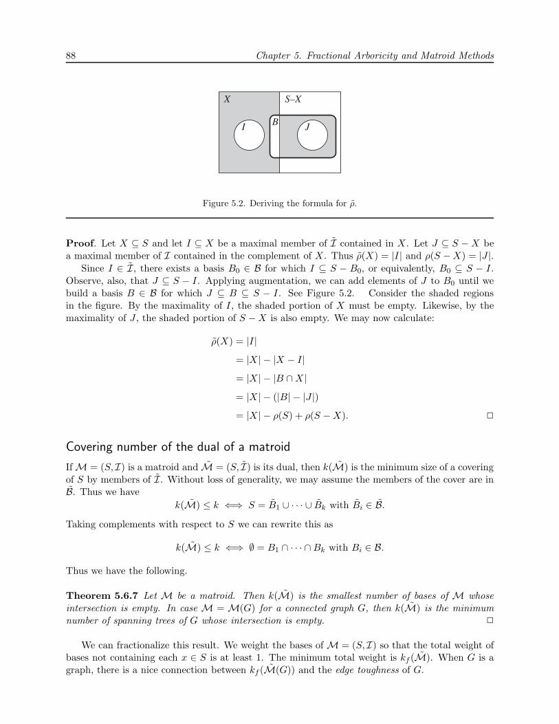
88 Chapter 5. Fractional Arboricity and Matroid Methods
X S–X
I JB
Figure 5.2. Deriving the formula for ρ.
Proof. Let X ⊆ S and let I ⊆ X be a maximal member of I contained in X. Let J ⊆ S −X bea maximal member of I contained in the complement of X. Thus ρ(X) = |I| and ρ(S −X) = |J |.
Since I ∈ I, there exists a basis B0 ∈ B for which I ⊆ S − B0, or equivalently, B0 ⊆ S − I.Observe, also, that J ⊆ S − I. Applying augmentation, we can add elements of J to B0 until webuild a basis B ∈ B for which J ⊆ B ⊆ S − I. See Figure 5.2. Consider the shaded regionsin the figure. By the maximality of I, the shaded portion of X must be empty. Likewise, by themaximality of J , the shaded portion of S −X is also empty. We may now calculate:
ρ(X) = |I|= |X| − |X − I|= |X| − |B ∩X|= |X| − (|B| − |J |)= |X| − ρ(S) + ρ(S −X). �
Covering number of the dual of a matroid
IfM = (S,I) is a matroid and M = (S, I) is its dual, then k(M) is the minimum size of a coveringof S by members of I. Without loss of generality, we may assume the members of the cover are inB. Thus we have
k(M) ≤ k ⇐⇒ S = B1 ∪ · · · ∪ Bk with Bi ∈ B.Taking complements with respect to S we can rewrite this as
k(M) ≤ k ⇐⇒ ∅ = B1 ∩ · · · ∩Bk with Bi ∈ B.
Thus we have the following.
Theorem 5.6.7 Let M be a matroid. Then k(M) is the smallest number of bases of M whoseintersection is empty. In case M =M(G) for a connected graph G, then k(M) is the minimumnumber of spanning trees of G whose intersection is empty. �
We can fractionalize this result. We weight the bases of M = (S,I) so that the total weight ofbases not containing each x ∈ S is at least 1. The minimum total weight is kf (M). When G is agraph, there is a nice connection between kf (M(G)) and the edge toughness of G.

5.6 Duality, duality, duality, and edge toughness 89
Edge toughness
Let G be a graph with at least one edge. The edge toughness of G is an invariant that measureshow resilient the graph is against edge deletion. Formally, the edge toughness of G, denoted σ′(G),is defined to be
σ′(G) = minF
|F |c(G− F )− c(G)
where the minimization is over all disconnecting subsets of edges of G. For example, if G is aconnected graph with edge toughness σ′, then we must delete at least �σ′j� edges to break G intoj + 1 components. This invariant is also known as the strength of the graph.
Now the denominator c(G−F )−c(G) is computable from the cycle matroid of G. If F ⊆ E(G),then ρ(F ) = n− c(V, F ) where n = |V (G)| and c(V, F ) is, of course, the number of components ofthe graph (V, F ). Thus
c(G− F )− c(G) = [n − c(G)] − [n− c(G − F )] = ρ(E) − ρ(E − F ).
Thus, letting X = E − F , we can rewrite the definition of edge toughness as
σ′(G) = minX
|E −X|ρ(E)− ρ(X)
where the minimization is over all subsets of edges X for which (V,X) has more components thanG.
Notice that this new definition easily extends to matroids. IfM = (S,I) is a matroid, define
σ′(M) = minX
|S −X|ρ(S)− ρ(X)
where the minimization is over all X ⊆ S for which ρ(X) < ρ(S).
Note that if G has at least one edge, then σ′(G) = 1 if and only if G has a cut edge (exercise 15on page 91). In a similar vein, Υ(G) =∞ if and only if G has a loop.
More generally, for a matroid M (with rank at least 1) we have σ′(M) = 1 if and only if Mhas a coloop (exercise 16), and Υ(M) =∞ if and only if M has a loop.
IfM has neither loops nor coloops, then there is a nice connection between σ′(M) and kf (M).
Theorem 5.6.8 Let M be a matroid and suppose both M and M are loopless. Then
1σ′(M)
+1
kf (M)= 1.
Proof. Rewrite Theorem 5.6.6 on page 87 as ρ(X) = |X|− ρ(S)+ ρ(S−X) and use it to compute:
1− 1σ′(M)
= 1−max(ρ(S)− ρ(X)|S −X|
)
= min(
1− ρ(S)− ρ(X)|S −X|
)
= min(
1− [|S| − ρ(S)]− [|X| − ρ(S) + ρ(S −X)]|S −X|
)
= min(
1− |S| − |X| − ρ(S −X)|S −X|
)

90 Chapter 5. Fractional Arboricity and Matroid Methods
= min(ρ(S −X)|S −X|
)
=1
kf (M). �
We can rewrite Theorem 5.6.8 in graph terms.
Corollary 5.6.9 Let G be a graph. The edge toughness of G is given by
σ′(G) =kf (M(G))
kf (M(G)) − 1.
If G is planar with planar dual G, then
σ′(G) =Υf (G)
Υf (G)− 1. �
In particular, the Matroid Partitioning Algorithm gives us a polynomial-time algorithm forcomputing the edge toughness of a graph.
5.7 Exercises
1. Prove that the arboricity of a planar graph is at most 3 and that this bound is the bestpossible.
2. Prove that mad(G) cannot be computed in a greedy fashion. Specifically, find a graph G forwhich the following algorithm fails.
Input: a graph G.
Output: (allegedly) mad(G).
(a) Let X ← ∅.(b) Let X ← X ∪ {d(G)}.(c) Let v be a vertex of minimum degree in G.
(d) Let G← G− v.(e) If G is not empty, go to step (b).
(f) Output the largest element of X.
3. Prove that for any matrix A, M(A) is indeed a matroid.
4. Prove that for any graph G, M(G) is indeed a matroid.
5. Create a good definition of isomorphic matroids.
6. Prove or disprove: For all graphs G, M(G) is isomorphic to M(A(G)) where A(G) is theadjacency matrix of G.
7. Prove or disprove: For every graph G, there is a matrix A so that M(G) is isomorphic toM(A).

5.8 Notes 91
8. Let Un,k denote the pair (S,I) where S is an n-set and I is the set of all subsets of S withat most k elements.
Prove that Un,k is a matroid. We call Un,k a uniform matroid.
Compute k(Un,k) and kf (Un,k).
9. Prove that there is no graph G for whichM(G) ∼= U4,2. (The preceding exercise defines Un,k.)
10. Prove that if ai, bi > 0 (for i = 1, . . . , c) then
a1 + · · ·+ ac
b1 + · · ·+ bc≤ max
i
{ai
bi
}.
(We use this fact in the proof of Theorem 5.1.1.)
11. Write a careful definition for t · M: the matroid formed from M by replacing each elementof the ground set ofM with t parallel elements.
12. Prove Lemma 5.5.1 on page 84: Let G be a connected graph. Then G has exactly one cycle ifand only if ν(G) = ε(G).
13. Let M = (S,I) be a matroid with rank function ρ. Let t be a positive integer. Define
It = {X ⊆ S : ρ(I) ≥ |I| − t},i.e., all sets that can be formed from independent sets by the addition of at most t additionalelements.
Prove that Mt = (S,It) is a matroid, called an elongation of M.
Observe that this is a generalization of Theorem 5.5.2 on page 84 since if M =M(G), thenM1 =M1(G).
14. Prove Theorem 5.6.5 on page 87: Let G be a planar graph (embedded in the plane) and let Gbe its dual. Then M(G) =M(G).
15. Let G be a graph with at least one edge. Prove that σ′(G) ≥ 1 and that σ′(G) = 1 if andonly if G has a cut edge.
16. (Generalizing the previous problem.) Let M be a matroid of rank at least 1. Prove thatσ′(M) ≥ 1 and σ′(M) = 1 if and only if M has a coloop.
17. Let M = (S,I) be a matroid. Define a hypergraph H = (S,I − {∅}), i.e., delete ∅ as amember of I. Note that k(M) = k(H). State and prove simple formulas for μ(H), p(H), andτ(H).
5.8 Notes
Matroids were invented by Hassler Whitney [189] in the 1930s. For background reading on matroids,see the monographs by Recski [152] or Welsh [186].
The results on arboricity (e.g., Theorem 5.1.1 on page 72) are due to Nash-Williams [137, 138].See also Edmonds [49].
The Matroid Partitioning Algorithm is due to Edmonds [49], but he treats a more generalsituation. Given several matroids on the same ground set, e.g., Mi = (S,Ii) for 1 ≤ i ≤ k,

92 Chapter 5. Fractional Arboricity and Matroid Methods
Edmonds seeks a partition S = I1 ∪ I2 ∪ · · · ∪ Ik where each Ii ∈ Ii. We only needed the case inwhich all k matroids are the same.
The material on fractional arboricity is based on the work of Payan [143] and Catlin, Grossman,Hobbs, and Lai [33, 34]. See the latter papers for a treatment of edge toughness.
Random graph theorists (and others) are concerned with graphs G whose densest portion isG itself. In particular, a graph G is called balanced provided mad(G) = d(G). Maximum averagedegree and balanced graphs arise in the theory of evolution of graphs. Let G be a fixed graph andlet n be a very large positive integer. Form a graph by gradually adding edges at random betweenn fixed vertices. As the density of the evolving random graph increases we eventually reach a stagewhere it is very likely that the random graph contains G as a subgraph. The point at which thishappens depends only on mad(G). See Bollobas [23] or Palmer [141]. For more information onbalanced graphs, see the papers by Lai and Lai [112] or Rucinski and Vince [155].

6
Fractional Isomorphism
6.1 Relaxing isomorphism
What does it mean for two graphs to be “the same”? The fundamental equivalence relation definedbetween graphs is that of isomorphism: graphs G and H are isomorphic, denoted G ∼= H, providedthere is a bijection φ : V (G)→ V (H) so that uv ∈ E(G) if and only if φ(u)φ(v) ∈ E(H). In otherwords, graphs G and H are isomorphic if they differ only in the names of their vertices.
In many branches of mathematics, it is useful to relax the notion of sameness. For example,in geometry, equality of figures is relaxed to congruence (isometry), which is further relaxed tosimilarity, or ultimately to the topological notion of homeomorphic.
We seek to relax the notion of graph isomorphism. To do so, let us recast graph isomorphism asan integer feasibility problem. Let G and H be graphs with adjacency matrices A and B. GraphsG and H are isomorphic if and only if there is a permutation matrix1 P so that A = PBP−1. Inother words, we can form the adjacency matrix A by applying the same permutation to both therows and columns of B; this amounts to relabeling the vertices of H to make G.
Now the relation A = PBP−1 can be rewritten as AP = PB. The requirement that P is apermutation matrix can be restated as (1) P · 1 = 1, (2) P t · 1 = 1, and (3) the entries of P are in{0, 1}. (Here and in the sequel, 1 stands for a vector of all 1’s.)
Thus, isomorphism of graphs G and H (with adjacency matrices A and B) is equivalent to thefeasibility of the following system of linear equations (think of A and B as given and the Pij ’s asthe unknowns):
AP = PB,
P · 1 = 1,
P t · 1 = 1, and
all Pij ∈ {0, 1}.Our theme has been to replace integer programs by linear programs, thus it is natural in this
setting to drop the requirement that P be a 0,1-matrix and simply require the entries in P to benonnegative. A matrix S whose entries are nonnegative, and whose rows and columns all sum to 1[i.e., S · 1 = 1 and St · 1 = 1] is called a doubly stochastic matrix.
We say that graphs G and H are fractionally isomorphic, and we write G ∼=f H, provided thereis a doubly stochastic matrix S for which AS = SB where A,B are the adjacency matrices of thegraphs G,H, respectively.
Proposition 6.1.1 The relation ∼=f is an equivalence relation.
Proof. Exercise 1 on page 108. �
1A permutation matrix P is a square 0,1-matrix with exactly one 1 in every row and column.
93

94 Chapter 6. Fractional Isomorphism
Figure 6.1. Two fractionally isomorphic graphs.
For example, let G and H be the two graphs in Figure 6.1. To verify that G ∼=f H, write theiradjacency matrices as
A =
⎡⎢⎢⎢⎢⎢⎢⎢⎢⎢⎢⎢⎢⎢⎢⎢⎢⎢⎢⎢⎢⎢⎣
011100 100000101010 010000110001 001000100011 000100010101 000010001110 000001100000 011000010000 101000001000 110000000100 000011000010 000101000001 000110
⎤⎥⎥⎥⎥⎥⎥⎥⎥⎥⎥⎥⎥⎥⎥⎥⎥⎥⎥⎥⎥⎥⎦
and B =
⎡⎢⎢⎢⎢⎢⎢⎢⎢⎢⎢⎢⎢⎢⎢⎢⎢⎢⎢⎢⎢⎢⎣
010101 100000101010 010000010101 001000101010 000100010101 000010101010 000001100000 010001010000 101000001000 010100000100 001010000010 000101000001 100010
⎤⎥⎥⎥⎥⎥⎥⎥⎥⎥⎥⎥⎥⎥⎥⎥⎥⎥⎥⎥⎥⎥⎦
.
(To check this, note that we have listed the six vertices of degree 4 (black in the figure) first andthe six vertices of degree 3 (white) last.) Let
S =(
16
) [J 00 J
]
where each J is a 6 × 6 matrix of all ones and each 0 is a 6 × 6 matrix of all zeros. It is obviousthat S is doubly stochastic, and (with a little work) one checks that AS = SB. Thus the graphsG and H are fractionally isomorphic. They are not, however, isomorphic. Notice that G is planar,but H is not (its black vertices induce a K3,3).
Although they are not isomorphic, these graphs have much in common. Let us note some ofthese common features, all of which hold in general for fractionally isomorphic graphs.

6.1 Relaxing isomorphism 95
• G and H have the same number of vertices (12).
• G and H have the same number of edges (21).
• Both have the same degree sequence (4, 4, 4, 4, 4, 4, 3, 3, 3, 3, 3, 3)
• Both have the same maximum eigenvalue (5+√
52 ≈ 3.61803).
These are not merely coincidences. Fractionally isomorphic graphs always share these commonattributes.
Proposition 6.1.2 Fractionally isomorphic graphs have the same number of vertices.
Proof. Check that doubly stochastic matrices must be square and the result follows easily. �
Proposition 6.1.3 Fractionally isomorphic graphs have the same number of edges.
Proof. Let A and B be the adjacency matrices of fractionally isomorphic graphs G and H, andlet S be doubly stochastic with AS = SB.
Notice that 1t ·A · 1 = 2ε(G) (we are summing the degrees of the vertices). Thus we compute
2ε(G) = 1t · A · 1= 1t · A(S · 1) because S is doubly stochastic
= 1t · (AS) · 1= 1t · (SB) · 1= (1t · S)B · 1= 1t · B · 1= 2ε(H). �
We prove below that fractionally isomorphic graphs share the same degree sequence (Proposi-tion 6.2.6 on page 98) and the same maximum eigenvalue (Proposition 6.5.2 on page 105).
In general, these conditions (same degree sequence, maximum eigenvalue, etc.) are not sufficientfor fractional isomorphism (see exercise 5 on page 108). However, we do have the following.
Proposition 6.1.4 Let G and H be r-regular graphs on n vertices. Then G ∼=f H.
Proof. Let A and B be the adjacency matrices of G and H. Let S = 1nJ where J is an n × n
matrix of all ones. Note that AS = rnJ = SB, hence G ∼=f H. �
Another view
There is another way to view isomorphism and fractional isomorphism. Let G and H be isomorphicgraphs on disjoint sets of vertices. Let us label the vertices of these graphs V (G) = {v1, . . . , vn}and V (H) = {w1, . . . , wn} so that vi �→ wi is an isomorphism.
We can think of this isomorphism as a perfect matching between V (G) and V (H), i.e., theisomorphism is represented by a 1-regular graph L on V (G) ∪ V (H). To distinguish the edge of Gand H from the edges of L, we call the edges in the bipartite graph L links. Let us now translate

96 Chapter 6. Fractional Isomorphism
the condition vivj ∈ E(G) ⇐⇒ wiwj ∈ E(H) into a statement about edges (of G and H) andlinks.
Let v ∈ V (G) and w ∈ V (H). We can find two sorts of 2-step paths from v to w. We might firsttake an edge of G followed by a link of L, or first take a link and then an edge (of H). These twokinds of paths are called edge-link or link-edge. The statement that L represents an isomorphismbetween G and H can be re-expressed as follows: For all v ∈ V (G) and all w ∈ V (H), there is alink-edge path from v to w if and only if there is an edge-link path from v to w.
We can describe fractional isomorphism in a similar way. LetG and H be graphs on n vertices asbefore, with adjacency matrices A and B respectively. Let S be doubly stochastic with AS = SB.The matrix S can be represented as a weighted bipartite graph L linking V (G) and V (H); there isa link from vi to wj just when Sij is positive. The weight of that link is, of course, Sij.
For the graphs in Figure 6.1 on page 94, the linking graph consists of two disjoint copies of K6,6
(one copy joining the black vertices and one copy joining the white vertices) in which every linkhas weight 1
6 . The condition AS = SB can be re-expressed as follows: For all vertices v ∈ V (G)and w ∈ V (H), the total weight of all links along edge-link paths from v to w equals the total weightof all links along link-edge paths from v to w.
6.2 Linear algebra tools
Our forthcoming analysis of fractional isomorphism relies on certain special properties of doublystochastic matrices. First, they are positive matrices and therefore their eigenvalues and eigenvec-tors have special properties (see Theorem 6.2.2 on the facing page). Second, they can be writtenas convex combinations of permutation matrices (see Theorem 6.2.3 on the facing page).
In this section we collect matrix results that are not part of most undergraduate linear algebracurricula. Experts who are tempted to skip this section should read Theorem 6.2.4 on page 98before proceeding.
Direct sum and reducibility
Let A and B be square matrices. The direct sum of A and B, denoted A⊕B, is the matrix
A⊕B =
[A 00 B
]
where each “0” represents a rectangular block of 0’s of the appropriate size. If M = A⊕B then wesay M is decomposable. More generally, we say M is decomposable if there exist matrices A, B, P ,and Q such that P and Q are permutation matrices and M = P (A⊕ B)Q. Otherwise (if no suchdecomposition exists) we say that M is indecomposable.
Let M be an n×n matrix. Let D(M) denote a digraph on n vertices v1, . . . , vn with an arc fromvi to vj just when Mij �= 0. We say that M is irreducible provided D(M) is strongly connected.Otherwise, we say that M is reducible. Notice that M is reducible just when there is a permutation
matrix P so that PMP t =
[A B0 C
]where A and C are square matrices and 0 is a rectangular
block of zeros.Furthermore, we say that a matrix M is strongly irreducible provided PM is irreducible for any
permutation matrix P . If M is not strongly irreducible, then we can find permutation matrices P
and Q so that PMQ =
[A B0 C
]where A and C are square matrices and 0 is a block of zeros.

6.2 Linear algebra tools 97
For example, the matrix
[0 11 0
]is irreducible, but neither strongly irreducible nor indecom-
posable.
Proposition 6.2.1 Let S be a doubly stochastic, indecomposable matrix. Then S is also stronglyirreducible.
Proof. Let S be a doubly stochastic matrix. We prove the contrapositive of the Proposition.Suppose S is not strongly irreducible, This means we can permute the rows and columns of S
so that S =
[S11 S12
0 S22
]where S11 and S22 are square matrices and 0 represents a rectangular
block of 0’s. We claim that S12 is 0. To see why, suppose S11 has shape a × a. Since S is doublystochastic, the sum of each column of S11 is 1, so the sum of all the entries in S11 is a. Now thesum of the entries in each row of [S11 S12] is also 1, so if any entry in S12 were nonzero, there wouldbe a row of S11 whose sum would be less than 1, implying that the sum of all the entries in S11
would be less than a, a contradiction. Thus S12 = 0 and it follows that S = S11 ⊕ S22, i.e., S isdecomposable. �
Positive matrices: the Perron-Frobenius theorem
Let M be a matrix. We write M ≥ 0 to mean that every entry in M is nonnegative and we saythat M is nonnegative. We write M > 0 if all of M ’s entries are positive, and we call M positive.Likewise, we may refer to vectors as being nonnegative or positive.
A dominant eigenvalue of a square matrix M is an eigenvalue λ of M whose absolute value isat least that of any other eigenvalue, i.e., if λ′ is also an eigenvalue of M , then |λ′| ≤ |λ|.
The principal theorem about nonnegative matrices is the celebrated Perron-Frobenius theorem.
Theorem 6.2.2 Let M be an irreducible, nonnegative matrix. Then M has a unique dominanteigenvalue λ which is positive and has an associated eigenvector that is positive. Further, eigenvec-tors associated with other eigenvalues are not nonnegative. �
Doubly stochastic matrices: Birkhoff decomposition
Permutation matrices are doubly stochastic. Furthermore, doubly stochastic matrices can be de-composed into permutation matrices as follows.
Theorem 6.2.3 Let S be a doubly stochastic matrix. There exist positive numbers α1, . . . , αs andpermutation matrices P1, . . . , Ps so that
S =s∑
i=1
αiPi and 1 =s∑
i=1
αi. �
This result can be expressed in words by saying every doubly stochastic matrix is a convexcombination of permutation matrices. The key step in the proof is graph-theoretic (see exercise 2on page 108). The decomposition S =
∑αiPi is known as a Birkhoff decomposition of the doubly
stochastic matrix S.The set of doubly stochastic matrices forms a compact, convex subset of the set of all real
matrices; the extreme points of this convex set are exactly the permutation matrices.

98 Chapter 6. Fractional Isomorphism
Let S be a doubly stochastic matrix and let x be a vector. The vector Sx is a list of weightedaverages of the entries in x. If R is another doubly stochastic matrix and R(Sx) = x, then, ineffect, no “loss of information” has taken place. Intuitively, this is only possible if Sx and x havethe same entries, i.e, Sx is just a permutation of x. Indeed, one can say more.
Theorem 6.2.4 Let S and R be n × n doubly stochastic matrices with Birkhoff decompositionsS =
∑αiPi and R =
∑βjQj. Let x,y be n-vectors.
(1) If y = Sx and x = Ry, then y = Pix and x = Qjy for all i, j.
(2) Let x and y be as in (1). If, in addition, either S or R is indecomposable, then x = y = s · 1for some scalar s.
(3) If x and y are 0,1-vectors and y = Sx, then y = Pix for all i.
The proof of this result makes use of the following convex set. Let v be a vector. Let Π(v) denotethe convex hull of all vectors formed by permuting the entries of v. Note that the extreme pointsof Π(v) are all the permutations of v, i.e., the vectors of the form Pv where P is a permutationmatrix (exercise 3 on page 108).
Now consider the statement y = Sx where S is doubly stochastic. Since S =∑αiPi, we have
y = Sx =∑αiPix and therefore y is a convex combination of permutations of x, i.e., y ∈ Π(x).
Furthermore, if P ′ is any permutation matrix, then P ′y = P ′Sx =∑αi(P ′Pi)x, so P ′y ∈ Π(x).
In short, all the extreme points of Π(y) are in Π(x); hence we have proved the following.
Lemma 6.2.5 If S is doubly stochastic and y = Sx, then Π(y) ⊆ Π(x). �
Proof (of Theorem 6.2.4). For (1), note that y = Sx and x = Ry imply, by Lemma 6.2.5, thatΠ(x) = Π(y). Thus x and y are extreme points of this polyhedron. As y =
∑αiPix we must have
that y = Pix for each i, and likewise x = Qjy for all j.For (2), first note that if either x or y is 0, then both are 0 and the conclusion follows. So
suppose that x,y are nonzero and that S is indecomposable. We know that y = Sx and thatx = Qy for some permutation matrix Q, thus x = QSx, i.e., x is an eigenvector of QS witheigenvalue 1. Note that the vector 1 also is an eigenvector with eigenvalue 1. Now S is nonnegativeand indecomposable, and hence strongly irreducible (by Proposition 6.2.1 on the preceding page),so QS is irreducible. Thus, by Theorem 6.2.2 on the preceding page, QS has a unique dominanteigenvalue which is positive and has an associated eigenvector that is positive. Thus it follows thatx is a scalar multiple of 1 as required.
For (3), we have only that y = Sx, but we also know that x,y ∈ {0, 1}n. Now we know thaty ∈ Π(x). Furthermore, 1ty = 1tSx = 1tx, so x and y have the same number of 1’s, i.e., x is apermutation of y. Thus y is an extreme point of Π(x) and therefore, since y =
∑αiPix we have
y = Pix for all i. �
As an application of Theorem 6.2.4, we prove that fractionally isomorphic graphs have the samedegree sequence. (In fact much more is true; see Theorem 6.5.1 on page 102.)
Proposition 6.2.6 If G ∼=f H, then G and H have the same degree sequence.
Proof. Let A,B be the adjacency matrices of G,H and let S be doubly stochastic with AS = SB.Let dG = A · 1 and dH = B · 1; these vectors record the degree sequences of G and H respectively.

6.2 Linear algebra tools 99
NowdG = A · 1 = AS · 1 = SB · 1 = SdH
anddH = B · 1 = BSt · 1 = StA · 1 = StdG
because BSt = StA follows from AS = SB by transposition. Thus by Theorem 6.2.4 on the facingpage we have that dH and dG are permutations of one another, i.e., G and H have the same degreesequence. �
Kronecker product
Let A and B be n×n matrices. The Kronecker product of A and B, denoted A⊗B, is the n2×n2
matrix ⎡⎢⎢⎢⎢⎣A11B A12B · · · A1nBA21B A22B · · · A2nB
......
. . ....
An1B An2B · · · AnnB
⎤⎥⎥⎥⎥⎦
where AijB denotes an n× n block formed by multiplying each entry of B by the scalar Aij.Matrices are convenient ways to represent linear transformations, so it is natural to seek a linear
transformation that A⊗B represents.For n× n matrices A, B, and X, let
FA,B(X) = AXBt.
Then FA,B is a linear transformation defined on the space Rn×n of all n× n real matrices.A natural basis for Rn×n is the set {E(i, j) : 1 ≤ i, j ≤ n} where E(i, j) is a matrix all of whose
entries are 0 except for a 1 in position ij. Note that FA,B(E(i, j)) = AE(i, j)Bt is a matrix whosep, q entry is given by
[AE(i, j)Bt]pq =∑a,b
ApaE(i, j)abBtbq = ApiBqj.
As p and q range over the numbers between 1 and n, we get the n2 entries in the jth column in theith block of columns in A⊗B.
Further, for an n× n matrix M , let c(M) denote the n2-column vector formed by stacking thecolumns of M one atop the next. We have
c (FA,B(X)) = (A⊗B)(c(X)).
Thus A⊗B is the matrix for the linear transformation FA,B with respect to the basis E(i, j).When A and B are doubly stochastic, we see that A⊗B is as well. Furthermore, we have the
following.
Lemma 6.2.7 Let A and B be doubly stochastic n × n matrices with Birkhoff decompositionsA =
∑i αiPi and B =
∑j βjQj . Then A ⊗ B is doubly stochastic with Birkhoff decomposition
A⊗B =∑
i,j αiβj(Pi ⊗Qj).
Proof. Check that if P and Q are permutation matrices, then so is P ⊗ Q. The lemma followseasily from there. �

100 Chapter 6. Fractional Isomorphism
6.3 Equitable partitions
The existence of a fractional isomorphism between two graphs is closely tied to the concept of anequitable partition of the vertices of a graph. To understand this concept, consider the black/whitecoloring of the graphs in Figure 6.1 on page 94. We mentioned earlier that the black vertices allhave degree 4 and the white vertices all have degree 3. Actually, much more is true. Observe thatevery black vertex has exactly 3 black neighbors and exactly 1 white neighbor. Note further thatevery white vertex has 1 black and 2 white neighbors.
Let S be a subset of the vertex set of a graph G. Let d(v, S) denote the degree of v in S, i.e.,the number of neighbors of v in S, i.e., d(v, S) = |N(v) ∩ S|.
We say that a partition V1∪· · ·∪Vs of V (G) is equitable provided that for all i, j and all x, y ∈ Vi
we have d(x, Vj) = d(y, Vj). In other words, each of the induced subgraphs G[Vi] must be regularand each of the bipartite graphs2 G[Vi, Vj ] must be biregular.3
Every graph has an equitable partition: form the partition in which every part is a single vertex.If G is a regular graph, then the partition with just one part containing all the vertices is equitable.
Now partitions of a set (including the equitable partitions of a graph) can be partially orderedby refinement.4 Given two partitions of a set P and Q, we can form their join, which is the finestpartition that is coarser than both P and Q. The join of P and Q is denoted P ∨Q.
Here is another way to describe the join of partitions P and Q. Let xP≡y mean that x and y
are in the same part of the partition P. It is easy to check thatP≡ is an equivalence relation. Let
R = P ∨Q. Then xR≡y if and only if we can find z1, z2, . . . , zs with
x ≡ z1 ≡ z2 ≡ · · · ≡ zs ≡ y
where each ≡ is eitherP≡ or
Q≡ (exercise 6 on page 109). The relationR≡ is the transitive closure of
the union of the relationsP≡ and
Q≡.
Lemma 6.3.1 Let P and Q be equitable partitions of a graph G. Then P ∨Q is also an equitablepartition.
Proof. Let R = {R1, . . . , Rr}. Note that each Ri can be partitioned into sets from P or into setsfrom Q (because P and Q are refinements of R).
Let x, y ∈ Ri. We must show that d(x,Rj) = d(y,Rj) for all j. To do this, note that it is
enough to consider the cases that xP≡y and x
Q≡y. Without loss of generality, suppose xP≡y.
Now Rj can be partitioned into sets from P, say Rj = P1 ∪ P2 ∪ · · · ∪ Pp where each Pa ∈ P.Thus
d(x,Rj) = d(x, P1) + · · · + d(x, Pp)
d(y,Rj) = d(y, P1) + · · · + d(y, Pp)
However, since x and y are in a common part of P it follows that d(x, Pa) = d(y, Pa) for all a, andthus d(x,Rj) = d(y,Rj) as required. �
2For disjoint A, B ⊆ V (G), we write G[A, B] to stand for the bipartite graph with vertex set A∪B in which thereis an edge from an A vertex to a B vertex iff that edge exists in G.
3A bipartite graph G = (X ∪ Y, E) is biregular if any two vertices in X have the same degree and if any twovertices in Y have the same degree (not necessarily the same as the degree of an X vertex).
4If P and Q are partitions of a common set S, we say that P is a refinement of Q provided every part of P is asubset of some part in Q. When P is a refinement of Q we also say that P is finer than Q and the Q is coarser thanP .

6.4 Iterated degree sequences 101
Theorem 6.3.2 Let G be a graph. Then G has a unique coarsest equitable partition.
Proof. Let P1, . . . ,Pk be a list of all of G’s equitable partitions; note that this list is nonemptysince the “all singletons” partition of V (G) is equitable. Let Q = P1 ∨ · · · ∨ Pk. By Lemma 6.3.1,Q is the unique coarsest equitable partition of G. �
The set of equitable partitions of a graph is a join semilattice. Since this semilattice has aminimum element (the all singletons equitable partition), it is a lattice; see exercise 7 on page 109.
Consider again the graphs in Figure 6.1 on page 94. We would like to say that they havea common equitable partition. Let us define what we mean by this. Let G be a graph and letP = {P1, . . . , Pp} be an equitable partition of V (G). The parameters of P are a pair (n,D) wheren is a p-vector whose ith entry is the size of Pi and D is a p × p matrix whose ij-entry is d(x, Pj)for any x ∈ Pi. For the graphs in Figure 6.1, the partitions into black and white vertices both haveparameters
n =
[66
]and D =
[3 11 2
].
We say that equitable partitions P and Q of graphs G and H have the same parameters if we canindex the sets in P and Q so that their parameters (n,D) are identical. In such a case we saythat G and H have a common equitable partition. If, in addition, P and Q are coarsest equitablepartitions of G and H, then we say that G and H have common coarsest equitable partitions.
The parameters (n,D) of an equitable partition P = {P1, . . . , Pp} of V (G) obey a few simplerelationships. First, since P is a partition of V (G), we have n1 + · · · + np = ν(G). Second, sincethe number of edges from part Pi to part Pj equals the number edges from part Pj to part Pi, wemust have niDij = njDji.
Furthermore, suppose we order the vertices of G so that vertices in P1 are listed first, thevertices in P2 second, etc. Then we can write the adjacency matrix A(G) as
A(G) =
⎡⎢⎢⎢⎢⎣A11 A12 · · · A1p
A21 A22 · · · A2p...
.... . .
...Ap1 Ap2 · · · App
⎤⎥⎥⎥⎥⎦
where block Aij is size ni × nj and the sum of each row of Aij is Dij .
6.4 Iterated degree sequences
Another concept central to an understanding of fractional isomorphism is that of the iterated degreesequence of a graph. Recall that the degree of a vertex v in G is the cardinality of its neighbor set:d(v) = |N(v)|. The degree sequence of a graph G is the multiset5 of the degrees of the vertices,
d1(G) = {d(v) : v ∈ V (G)}.
(The reason for the subscript ‘1’ will become apparent shortly.)
5Usually, the degree sequence of a graph is a list of the degrees, often in descending numerical order. For ourpurposes here, however, the multiset formulation is more useful.

102 Chapter 6. Fractional Isomorphism
We can also define the degree sequence of a vertex to be the multiset of the degrees of itsneighbors:
d1(v) = {d(w) : w ∈ N(v)}.For the graphs in Figure 6.1 on page 94, the white vertices have degree sequence {3, 3, 4} and theblack vertices have degree sequence {3, 4, 4, 4}.
The degree sequence sequence of G is simply the multiset of degree sequences of the vertices ofG:
d2(G) = {d1(v) : v ∈ V (G)}.Likewise, the degree sequence sequence of a vertex is the multiset of degree sequences of its neighbors:
d2(v) = {d1(w) : w ∈ N(v)}.For the graphs in Figure 6.1 the white vertices w and the black vertices b have
d2(w) ={{3, 3, 4}, {3, 3, 4}, {3, 4, 4, 4}
}, and
d2(b) ={{3, 3, 4}, {3, 4, 4, 4}, {3, 4, 4, 4}, {3, 4, 4, 4}
}.
There is, of course, no reason to stop here. In general, define:
d1(G) = {d(v) : v ∈ V (G)},d1(v) = {d(w) : w ∈ N(v)},
dk+1(G) = {dk(v) : v ∈ V (G)}, and
dk+1(v) = {dk(w) : w ∈ N(v)}.Finally, we may define the ultimate degree sequence of a vertex v or a graph G to be the infinite
lists:
D(v) = [d1(v), d2(v), . . .] , and
D(G) = [d1(G), d2(G), . . .] .
Notice that for the example graphs of Figure 6.1 on page 94 we have D(H) = D(G). Indeed,the equivalence between having a fractional isomorphism, having a common coarsest equitablepartition, and having the same ultimate degree sequence is the main theorem about fractionalisomorphism.
6.5 The main theorem
Theorem 6.5.1 Let G and H be graphs. The following are equivalent.
(1) G ∼=f H.
(2) G and H have a common coarsest equitable partition.
(3) G and H have some common equitable partition.
(4) D(G) = D(H).
6.5 The main theorem 103
Proof. Let G and H be graphs on n vertices with disjoint vertex sets V (G) = {v1, . . . , vn} andV (H) = {w1, . . . , wn}. Let A and B denote their respective adjacency matrices.
We first show (1)⇒ (3). We use that to prove (1)⇒ (2), while (2)⇒ (3) is trivial. From there,we go on to show (3)⇒ (1), (3)⇒ (4), and (4)⇒ (3).
(1)⇒ (3): Suppose G ∼=f H and let S be doubly stochastic with AS = SB. By suitably renamingthe vertices ofG and/orH, we may assume that S has block structure S = S1⊕· · ·⊕Ss where each Si
is indecomposable (and therefore, by Proposition 6.2.1 on page 97, each Sk is strongly irreducible).The matrix S induces partitions on the vertices of G and H as follows. Let PG = {V1, . . . , Vs} bethe partition of G in which vi and vj are in the same part just when indices i and j both fall insidethe scope of the same Sk. Let PH = {W1, . . . ,Ws} be the partition of H defined in the same way.
We show that PG and PH are equitable partitions with the same parameters.We may partition the adjacency matrices A and B into blocks Aij and Bij following the parti-
tions PG and PH . The condition AS = SB can be expanded to read⎡⎢⎢⎢⎢⎣A11 A12 · · · A1s
A21 A22 · · · A2s...
.... . .
...As1 As2 · · · Ass
⎤⎥⎥⎥⎥⎦
⎡⎢⎢⎢⎢⎣S1 0 · · · 00 S2 · · · 0...
.... . .
...0 0 · · · Ss
⎤⎥⎥⎥⎥⎦ =
⎡⎢⎢⎢⎢⎣S1 0 · · · 00 S2 · · · 0...
.... . .
...0 0 · · · Ss
⎤⎥⎥⎥⎥⎦
⎡⎢⎢⎢⎢⎣B11 B12 · · · B1s
B21 B22 · · · B2s...
.... . .
...Bs1 Bs2 · · · Bss
⎤⎥⎥⎥⎥⎦ .
This can be rewritten more compactly as
AijSj = SiBij. (∗)
Transposing AS = SB yields StA = BSt, which can be expressed
StiAij = BijS
tj . (∗∗)
The vector dij(G) = Aij · 1 gives the number of edges from each vertex in Vi to all vertices inVj and the vector dij(H) = Bij · 1 gives the number of edges from each vertex in Wi to all verticesin Wj. We are done once we show that dij(G) = dij(H) = c · 1 for some integer c.
To do this, multiply equations (∗) and (∗∗) on the right by the vector 1 to get
AijSj · 1 = SiBij · 1⇒ dij(G) = Sidij(H), and
StiAij · 1 = BijS
tj · 1⇒ St
idij(G) = dij(H).
We may now apply part (2) of Theorem 6.2.4 on page 98 to vectors dij(G) and dij(H) to concludethat dij(G) = dij(H) = c · 1 as required.
(1) ⇒ (2): We have shown that (1) ⇒ (3). Further, we have shown that the blocks of S induce acommon equitable partition in the graphs G and H. We use this to show that (1)⇒ (2).
Suppose G ∼=f H and S is doubly stochastic with AS = SB. Let PG be the coarsest equitablepartition of G with parameters (n,D). It is enough to show that H has an equitable partition withthe same parameters.

104 Chapter 6. Fractional Isomorphism
Let PG = {V1, . . . , Vr} and assume that we have labeled the vertices of G so that the first n1
vertices of G are in V1, the next n2 vertices of G are in V2, etc.Let Ri = (1/ni)Jni where ni = |Vi| and Jni is an ni × ni block of all ones. Put R = R1 ⊕R2 ⊕
· · · ⊕Rr. Note that R is doubly stochastic. Furthermore, because PG is an equitable partition, wehave that niDij = njDji, which we rearrange to read AR = RA.
Since AS = SB, we compute that ARS = RAS = RSB.Next we claim that RS = R. We know that the indecomposable blocks of S correspond to a
(perhaps finer) equitable partition of G; thus we may write S = S1⊕S2⊕ · · ·⊕Sr where each Sk isdoubly stochastic (but not necessarily indecomposable) and has the same dimensions as Rk. ThusRS = (R1S1)⊕ · · · ⊕ (RrSr) and RkSk = Rk because Rk is a scalar multiple of a matrix of all onesand Sk is doubly stochastic.
Since we know that ARS = RSB, we now have AR = RB. We therefore know that R inducesan equitable partition in H with the same parameters as PG, and we are done.
(2)⇒ (3): Trivial.
(3) ⇒ (1): Suppose G and H have equitable partitions PG and PH with the same parameters(n,D). Let PG = {V1, . . . , Vs}, PH = {W1, . . . ,Ws} labeled so that |Vi| = |Wi| = ni and so thatthe number of edges from any vertex in Vi to Vj or from any vertex in Wi to Wj is Dij . Furthermore,we may assume that the vertices of G are labeled so that the first n1 vertices are in V1, the nextn2 vertices are in V2, etc., and the same for H and W1,W2, . . ..
Let Si = (1/ni)Jni and let S = S1⊕ · · · ⊕Ss. Now just check that the doubly stochastic matrixS satisfies AS = SB, hence G ∼=f H.
(3) ⇒ (4): Let PG = {V1, . . . , Vs} and PH = {W1, . . . ,Ws} be equitable partitions of G and Hwith the same parameters. We want to show that D(G) = D(H). It is enough to show that for allv,w ∈ Vi ∪Wi we have D(v) = D(w), i.e., dk(v) = dk(w) for all k. We do this by induction on k.
The basis case k = 1 follows from the fact that PG and PH are equitable partitions with thesame parameters. Suppose we know that for all v,w ∈ Vi ∪Wi we have dk−1(v) = dk−1(w). Nowdk(v) = {dk−1(x) : x ∈ N(v)} and dk(w) = {dk−1(y) : y ∈ N(w)}. But we know that the numberof neighbors of v and w in each part of the appropriate partition is the same, so by induction wehave dk(v) = dk(w).
(4) ⇒ (3): Suppose D(G) = D(H). Partition both G and H putting two vertices in the samepart if they have the same iterated degree sequence; call these partitions PG and PH . From thevector D(v) we can read off how many neighbors of each type v has. It follows that PG and PH
are equitable with the same parameters. �
Some consequences
Theorem 6.5.1 on page 102 has some interesting consequences. We list them briefly here.
Let G and H be graphs. They are fractionally isomorphic just when their coarsest equitablepartitions have the same parameters. Thus we can test if G and H are fractionally isomorphic byfinding their coarsest equitable partitions (see exercise 12 on page 109) and then comparing theparameters of the two partitions.

6.6 Other relaxations of isomorphism 105
Let P = {V1, . . . , Vp} and Q = {W1, . . . ,Wp} be coarsest equitable partitions of fractionallyisomorphic graphs G and H. We see from the proof of Theorem 6.5.1 that we may assume that thedoubly stochastic matrix S has the form S = (1/n1)Jn1 ⊕ · · · ⊕ (1/np)Jnp . Thus we may assumethat the linking graph is a disjoint union of complete bipartite graphs with uniform edge weights.
Further, if we partition the adjacency matrix A of G according to the coarsest equitable parti-tion, i.e.,
A =
⎡⎢⎣A11 · · · A1p...
. . ....
Ap1 · · · App
⎤⎥⎦
then we know that Aij is a 0,1-matrix with constant row sum dij (and constant column sum dji).We can form all graphs fractionally isomorphic to G by the following operation: For every pair ofindices i, j with 1 ≤ i ≤ j ≤ p, replace Aij by any 0,1-matrix Cijof the same shape with the samerow and column sums (and replace Aji = At
ij with Ctij). This gives a complete description of the
fractional isomorphism class of a graph.
Let P = {V1, . . . , Vp} be the coarsest equitable partition of G. For any two vertices x, y in thesame part of P the number of walks of length k starting at x must equal the number of walks oflength k starting at y. Further, if G is fractionally isomorphic to H, then for any vertex z linkedto x, the number of walks starting at z of length k (in H) must equal the the number of length kwalks (in G) starting at x.
Let w(k) denote the vector of the number of walks of length k starting anywhere in G. Notethat w(k) = Ak · 1. If G is connected, Ak · 1 tends to the eigendirection corresponding to thelargest eigenvalue λ of A. Thus for any vertex x, the number of walks of length k starting at x isasymptotic to cλk for some positive constant c. (If the graph is not connected, the number of walksof length k out of a vertex grows like λk where λ is the maximum eigenvalue of the component ofthe graph containing the vertex.)
We have thus proved the following.
Proposition 6.5.2 If G ∼=f H then the maximum eigenvalues of G and H are the same. �
Note that fractionally isomorphic graphs need not be cospectral; see exercise 10 on page 109.
6.6 Other relaxations of isomorphism
The relation G ∼= H is equivalently expressed in matrix notation as AP = PB or A = PBP t whereP is a permutation matrix; the equivalence follows from the fact that P t = P−1, i.e., permutationmatrices are real orthogonal matrices. However, it is not necessarily the case that St = S−1 for adoubly stochastic matrix. Thus the condition that A = SBSt for some S is not equivalent to thecondition that AS = SB for some S.
Define a relation → on square matrices by A → B provided A = SBSt for some doublystochastic matrix S. Furthermore, let us write A ↔ B provided A = SBSt and B = StAS forsome doubly stochastic matrix S.
Surprisingly, the relations → and ↔ on adjacency matrices are the same and are equivalent toisomorphism!
Theorem 6.6.1 Let G and H be graphs with adjacency matrices A and B. The following areequivalent.

106 Chapter 6. Fractional Isomorphism
(1) G ∼= H.
(2) A↔ B.
(3) A→ B and B → A.
(4) A→ B.
Note that the relations → and ↔ are not the same for general square matrices and, in general,→ is not an equivalence relation. For example, let I be a 2×2 identity matrix and let B = 1
2J2, the2× 2 matrix all of whose entries are 1/2. Then A→ B but B �→ A and A↔� B. In Theorem 6.6.1the equivalences hold because the entries of the matrices are in {0, 1}.
Proof. The implications (1)⇒ (2)⇒ (3)⇒ (4) are all trivial. We show (4)⇒ (1).Recall the material on Kronecker product (see page 99). The relation A → B can be restated
as A = FS,S(B) for some doubly stochastic matrix S. Let S =∑
i αiPi be a Birkhoff decompositionof S. Apply part (3) of Theorem 6.2.4 on page 98 and we have that A = FPi,Pj(B) for all i, j. Inparticular, if we take i = j we have A = PiBP
ti and therefore G ∼= H. �
Theorem 6.6.1 gives an interesting approach to checking if two graphs are isomorphic. One cancheck if the following system of quadratic equations, linear equations, and linear inequalities hold:
A = SBSt,
S · 1 = 1,
St · 1 = 1, and
S ≥ 0.
Of course, checking the feasibility of a general system of quadratic equations is a difficult problem.
Semi-isomorphism
We relaxed the equation A = PBP t by allowing P to stand for a doubly stochastic matrix insteadof a permutation matrix. A further relaxation is to allow the two instances of P to stand fordifferent doubly stochastic matrices. Let us say that graphs G and H (with adjacency matrices Aand B) are semi-isomorphic, G ∼=′ H, provided there are doubly stochastic matrices R and S sothat A = SBR.
It is not obvious that ∼=′ is an equivalence relation. However, this fact is a consequence of thefollowing.
Lemma 6.6.2 Let G and H be graphs with adjacency matrices A and B. Then G ∼=′ H if andonly if there are permutation matrices P and Q so that A = PBQ.
Proof. The (⇐) implication is trivial. For the (⇒) implication let G and H be semi-isomorphicwith A = SBR. We can write this as A = FS,Rt(B). Applying part (3) of Theorem 6.2.4 on page 98we have A = FP,Qt(B) where P and Q are permutation matrices in Birkhoff representations of Sand R respectively. Thus A = PBQ as claimed. �

6.6 Other relaxations of isomorphism 107
If A = PBQ for permutation matrices P and Q, then we have
QAQt = Q(PBQ)Qt = (QP )B.
In other words, after suitably renaming the vertices of G, we see that the adjacency matrix of Ghas the identical rows as the adjacency matrix of H, but perhaps in a different order. In otherwords, the neighborhoods of G and H are the same. Let’s make this more precise.
Let G be a graph. For v ∈ V (G) its neighborhood is, of course, N(v) = {w ∈ V (G) : vw ∈E(G)}. Define the neighborhood multiset of G to be the multiset N(G) = {N(v) : v ∈ V (G)}.
Thus graphs G and H are semi-isomorphic if and only if we can relabel their vertices so thatN(G) = N(H).
Semi-isomorphism lives somewhere between isomorphism and fractional isomorphism.
Theorem 6.6.3 Let G and H be graphs. Then
G ∼= H ⇒ G ∼=′ H ⇒ G ∼=f H.
Furthermore, neither implication may be reversed.
Proof. The first implication is trivial. For the second, let A and B be the adjacency matrices ofgraphs G and H, and (using Lemma 6.6.2) let P and Q be permutation matrices with A = PBQ.Taking transposes we have A = QtBP t. These equations can be rewritten
AQt = PB
AP = QtB.
Adding these equations and dividing by two gives AS = SB, where S = 12(P + Qt) is doubly
stochastic. Hence G ∼=f H. The fact that neither implication can be reversed is left to the reader(exercise 11 on page 109). �
The semi-isomorphism of graphs can be related to the isomorphism of bipartite graphs as follows.Let G be a graph with V (G) = {v1, . . . , vn}. Associate with G a bipartite graph B(G). The
vertices of B(G) are {x1, . . . , xn, y1, . . . , yn}. We have an edge xiyj in B(G) just when vivj ∈ E(G).
If A is the adjacency matrix of G, then the adjacency matrix of B(G) is
[0 AA 0
]. Notice that for a
bipartite graph G, we have B(G) ∼= 2G (2 disjoint copies of G). See also the proof of Theorem 2.1.6on page 16.
Theorem 6.6.4 Let G and H be graphs. Then G ∼=′ H if and only if B(G) ∼= B(H).
Proof. Let G and H be graphs with adjacency matrices A and B.If G ∼=′ H then we can find permutation matrices P and Q so that A = PBQ. Check that
[0 AA 0
]=
[P 00 Qt
]·[
0 BB 0
]·[P t 00 Q
]
and therefore B(G) ∼= B(H).

108 Chapter 6. Fractional Isomorphism
Now suppose B(G) ∼= B(H). Consider first the case that B(G) and B(H) are connected. Since
B(G) and B(H) are isomorphic there is a permutation matrix
[P QR S
]so that
[0 AA 0
]=
[P QR S
]·[
0 BB 0
]·[P t Rt
Qt St
].
Now an isomorphism between connected bipartite graphs preserves (or reverses) the bipartitionof the graph. Thus either P = S = 0 (and Q and R are permutation matrices) or Q = R = 0(and P and S are permutation matrices). We know from the above matrix equation that A =PBSt +QBRt. In case P = S = 0 we have A = QBRt and in case Q = R = 0 we have A = PBSt.In either case, we conclude that G ∼=′ H.
If B(G) and B(H) are not connected, we simply repeat the above analysis for their pairs ofisomorphic components. �
The semi-isomorphism of graphs reduces to isomorphism of bipartite graphs. For bipartitegraphs, isomorphism and semi-isomorphism are the same.
Corollary 6.6.5 If G and H are bipartite, then G ∼= H ⇐⇒ G ∼=′ H.
Proof. G ∼=′ H ⇐⇒ B(G) ∼= B(H) ⇐⇒ 2G ∼= 2H ⇐⇒ G ∼= H. �
6.7 Exercises
1. Prove that ∼=f is an equivalence relation. (Hint: First prove that if S and T are n×n doublystochastic matrices, then so is ST .)
2. Let S be a doubly stochastic matrix. Let B(S) be the bipartite graph whose vertices corre-spond to the rows and columns of S, in other words, V (B(S)) = {r1, r2, . . . , rn, c1, c2, . . . cn}.Put an edge from ri to cj just when Sij �= 0.
Prove that B(S) has a perfect matching.
Use this to prove that S can be written as a convex combination of permutation matrices(Theorem 6.2.3 on page 97).
3. Let v be a vector and let
X = {Pv : P is a permutation matrix}.
Thus Π(v) = 〈X〉, i.e., the convex hull of the points in X. Prove that X is the set of extremepoints of Π(v).
Restated, prove that if v =∑αiPiv where the αi’s are positive and sum to one, then Piv = v
for all i.
4. Prove that if G is a graph and T is a tree and if G ∼=f T , then G ∼= T .
5. Show that the eigenvalues and the degree sequences of the two graphs in Figure 6.2 on thefacing page are the same, but the graphs are not fractionally isomorphic.

6.7 Exercises 109
Figure 6.2. Two graphs with the same degree sequence and eigenvalues but that are not fractionally isomor-phic.
6. Let P, Q, and R be partitions of a set S. Suppose R = P ∨Q. Choose x, y ∈ S. Prove that
xR≡y if and only if there exist z1, . . . , zs ∈ S so that
x ≡ z1 ≡ z2 ≡ · · · ≡ zs ≡ y
where each ≡ is eitherP≡ or
Q≡. Indeed, show that we may assume that the ≡ alternatebetween
P≡ andQ≡.
7. Let P = (X,≤) be a finite partially ordered set in which the join of any two elements isdefined. Suppose also that P has a minimum element (an element that is below all otherelements). Prove that the meet of any two elements of P is also defined and therefore P is alattice.
(The meet of x and y, denoted x ∧ y, is the greatest element that is below both x and y. Alattice is a partially ordered set in which the meet and join of any two elements are defined.)
8. Let G be a graph and let P and Q be equitable partitions of G. Is it necessarily the case thatthe coarsest common refinement of P and Q is equitable?
9. What is the relationship between the tensor product of vectors v ⊗ w and the Kroneckerproduct of matrices A⊗B?
10. In Proposition 6.5.2 on page 105 we learn that maximum eigenvalue is a fractional isomor-phism invariant. Find a pair of fractionally isomorphic graphs that are not cospectral (havethe same eigenvalues).
11. Show that neither implication in Theorem 6.6.3 on page 107 can be reversed. That is (1) finda pair of graphs that are semi-isomorphic, but not isomorphic, and (2) find a pair of graphsthat are fractionally isomorphic, but not semi-isomorphic.
12. Let G be a graph and let P = {V1, . . . , Vp} be a partition of V (G). Form a new partition P ′
as follows: two vertices x, y ∈ Vi will be in a common part of P ′ just when d(x, Vj) = d(y, Vj)for all j.

110 Chapter 6. Fractional Isomorphism
Consider the sequence P → P ′ → P ′′ → · · · beginning with the partition P = {V (G)}, i.e.,the one-part partition of V (G).
Prove that the sequence leads to the coarsest equitable partition of G at which point allfurther partitions are the same.
13. Is the problem of deciding whether two given graphs are fractionally isomorphic solvable inpolynomial time, or is this decision problem NP-complete?
14. Let G be a graph. Let G′ denote the bipartite graph formed from G by replacing each edgeof G by a path length 2. (In other words, we form G′ from G by subdividing each edge of G.)
Prove that G ∼= H ⇐⇒ G′ ∼= H ′.
Conclude that the problem of recognizing a pair of isomorphic graphs is polynomially equiv-alent to the problem of recognizing a pair of semi-isomorphic graphs.
15. Let G be a graph with adjacency matrix A. A fractional automorphism of G is a doublystochastic matrix S so that AS = SA.
Prove that the set of fractional automorphisms of G forms a semigroup under matrix multi-plication.
6.8 Notes
This chapter is based largely on the paper [151] by Ramana, Scheinerman, and Ullman. The notionsof fractional isomorphism and equitable partitions can be traced back to the work of Brualdi [32],Leighton [116], McKay [130], Mowshowitz [135], and Tinhofer [177].
For background on Theorem 6.2.2 on page 97, commonly known as the Perron-Frobenius The-orem, see [95] and [96]. Theorem 6.2.4 on page 98 is due to Hardy, Littlewood, and Polya [84]. Seealso Rado [150] as well as the book by Marshall and Olkin [128].
The graphs in Figure 6.2 on the preceding page are courtesy of Allen Schwenk.Armed with the notion of fractional isomorphism, one can seek to prove a fractional version
of the reconstruction problem; see the survey articles by Bondy [24] or Nash-Williams [139] for anoverview. The fractional reconstruction problem is tantamount to the reconstruction of iterateddegree sequences. This was considered by Manvel [127] and remains an open problem.
The computational complexity of graph isomorphism is unknown; clearly the problem is in NP,but it is not known if it is NP-hard or polynomial-time solvable. Booth and Colbourn [27] showthat checking if bipartite graphs are isomorphic is just as hard as checking if general graphs areisomorphic. Thus the semi-isomorphism problem is again as hard as graph isomorphism. However,determining if two graphs are fractionally isomorphic is polynomial-time solvable.

7
Fractional Odds and Ends
7.1 Fractional topological graph theory
Topological graph theory deals with finding “best” drawings of graphs on various surfaces. Onemay wish to minimize the genus of the surface, or the number of crossings. Or one may seek todecompose the graph into a minimum number of planar subgraphs. These ideas correspond to thegraph invariants known as genus, crossing number, and thickness. We consider fractional analoguesof each.
Fractional genus
The genus g(G) of a graph G is the smallest genus of an oriented surface on which G can beembedded. Planar graphs have genus 0, nonplanar graphs that are embeddable on the torus havegenus 1, and so forth. In searching for an interesting fractional analogue of this notion, one is lednaturally to the following: Write tG for the graph composed of t disjoint copies of G, and thendefine the fractional genus gf (G) of a graph G by limt→∞ g(tG)/t. Unfortunately, this definitioncollapses completely, yielding gf = g for all graphs, owing to the following.
Theorem 7.1.1 The genus of a graph is the sum of the genera of its components. �
Thusgf (G) = lim
t→∞g(tG)t
= limt→∞
tg(G)t
= g(G).
The situation for nonorientable genus is more complicated. The nonorientable genus of a nonori-entable surface is the number of crosscaps one must add to a sphere to achieve that surface. Thesurface with nonorientable genus 1 is called the projective plane. The nonorientable genus of agraph G, denoted g(G), is the least nonorientable genus of a nonorientable surface upon which Gembeds. The fractional nonorientable genus of G is, of course,
gf (G) = limt→∞
g(tG)t
.
The nonorientable analogue of Theorem 7.1.1 fails. For example, g(K7) = 3, but g(2K7) = 5 �=3 + 3.
It is known that g(G) ≤ 2g(G) + 1 for any graph G, but no lower bound can be given on g(G)in terms of g(G) as there are graphs of arbitrarily high genus that embed on the projective plane(so g(G) is large with g(G) = 1). Of course, g(G) = 0 if and only if g(G) = 0 if and only if G isplanar.
Graphs G for which g(G) = 2g(G) + 1 are called orientably simple. The relationship betweeng(tG) and g(G) depends on whether G is orientably simple.
111

112 Chapter 7. Fractional Odds and Ends
Theorem 7.1.2 Let G be a graph and let t be a positive integer. Then g(tG) = t(g(G)− 1) + 1 incase G is orientably simple, and g(tG) = tg(G) otherwise. �
This gives the following corollary.
Corollary 7.1.3 Let G be a graph. Then gf (G) = g(G) − 1 in case G is orientably simple, andgf (G) = g(G) otherwise. �
Fractional crossing number
Let G be a graph. If G is planar, then it can be drawn in the plane without edge crossings.Otherwise any drawing of G must have crossings. The crossing number of G, denoted x(G), is theminimum number of crossings in any drawing of G.
There is a natural way to fractionalize the crossing number.Let t ·G denote the multigraph formed from G by replacing each edge by t parallel copies.Let xt(G) = x(t ·G). Note that x1(G) = x(G) and that xt(G) ≤ t2x(G) by simply drawing t ·G
with each edge replaced by t nearly identical curves. Each crossing in the old drawing becomes t2
crossings in the new.Let xf (G) = limt→∞ xt(G)/t2. The existence of this limit is guaranteed by the following result,
from which it follows also that xf (G) is nothing more than x(G).
Theorem 7.1.4 For any graph G and any positive integer t, xt(G) = t2x(G).
Proof. Prepare a drawing of t ·G with the fewest possible crossings, say k = xt(G) = x(t ·G). Weknow that k ≤ t2x(G).
Define a selection S of t · G to be a copy of G formed by taking one edge from each family ofparallel edges. Clearly there are tm possible selections where m = |E(G)|. A crossing X is a pairof edges of t · G that cross. A crossing X is said to belong to a selection S provided both edgesin X are in S. Finally, let Σ denote the set of all ordered pairs (X,S) where X is a crossing thatbelongs to a selection S. We ask, What is the cardinality of Σ? We count in two different ways:
• |Σ| ≥ tmx(G): For each selection S there are at least x(G) crossings belonging to thatselection.
• |Σ| = ktm−2. For each of the k = x(t ·G) crossings X in the drawing of t ·G there are tm−2
selections that include the edges in X (since we have chosen the two edges in X but the otherm− 2 edges may be chosen freely).
Thereforetmx(G) ≤ ktm−2
and so k ≥ t2x(G) as required. �
Fractional thickness
The thickness of a graph G, denoted θ(G), is the minimum number of planar graphs whose (edge)union is G. In other words, if G = (V,E) we seek to decompose E = E1∪E2∪· · · ∪Ek so that each(V,Ei) is a planar graph. The least k for which such a decomposition is possible is the thickness.
In hypergraph language, given a graph G = (V,E), form a hypergraph H whose vertices arethe edges of G. A collection F of edges of G (vertices of H) form a hyperedge just when (V, F ) isplanar. Then the thickness of G is just the covering number of H, i.e., θ(G) = k(H).

7.2 Fractional cycle double covers 113
We therefore define the fractional thickness of G to be θf (G) = kf (H).Note that (fractional) thickness is much like (fractional) arboricity (see Chapter 5), but the
hypergraph H defined above does not necessarily have a matroid structure; see exercise 1 onpage 128. However, the following is clear.
Lemma 7.1.5 For any graph G we have θ(G) ≤ Υ(G) and θf (G) ≤ Υf (G).
Proof. Decomposing G into forests certainly decomposes G into planar subgraphs. �
For complete graphs Kn the following result is known.
Theorem 7.1.6 For n �= 9, 10 we have θ(Kn) = �(n + 7)/6�, but θ(K9) = θ(K10) = 3. �
For fractional thickness we know the following.
Theorem 7.1.7 For all n ≥ 3 we have θf (Kn) =(n2
)/(3n − 6).
Proof. Note thatKn is edge-transitive, hence its associated hypergraph is vertex-transitive. There-fore we may apply Proposition 1.3.4 on page 5. Since a maximum planar subgraph of Kn has 3n−6edges, the result follows. �
The reader is invited to verify (exercise 2 on page 128) that for all n ≥ 3 we have θ(Kn) =�θf (Kn)� except for n = 9, 10.
7.2 Fractional cycle double covers
Let G be a graph. A cycle double cover (CDC, for short) for G is a family (i.e., a multiset) of cyclesin G with the property that every edge of G is in exactly two members of the family. Clearly, if Ghas a cut edge then no CDC of G is possible. However, it is believed that all other graphs admit aCDC.
Conjecture 7.2.1 (CDC) Every 2-edge-connected graph has a cycle double cover. �
If every block of a graph has a cycle double cover, then these covers, taken together, give a CDCfor the entire graph. Thus, to prove the CDC conjecture, it is enough to show that all 2-connectedgraphs admit CDCs.
It is easy to check (exercise 3 on page 128) that if a graph is Eulerian, then it has a CDC.The CDC conjecture is related to graph embedding. Let G be a 2-connected planar graph.
Then every face of (an embedding of) G is a simple cycle and every edge of G is in exactly twofaces. Thus the facial cycles of G form a cycle double cover, and hence the CDC conjecture is truefor planar graphs. For a general 2-connected graph G, if G embeds on a surface S so that everyface is bounded by a simple cycle of G, then the same argument works.
Because the cycle double cover problem is a covering problem, it admits a natural fractional-ization. Let G be a graph and let M be a matrix whose rows are indexed by the edges of G andwhose columns are indexed by the cycles of G. Let the i,j-entry of M be a 1 in case the ith edgelies in the jth cycle of G, and 0 otherwise. Then a CDC corresponds to a nonnegative, integervector x so that Mx = 2 (where 2 stands for a vector of all 2s). To fractionalize, we simply dropthe integrality condition.
Stated another way, a fractional cycle double cover of G assigns a (nonnegative, real) weight toevery cycle of G so that the sum of the weights of the cycles containing any given edge is exactlytwo. The natural fractional version of the CDC conjecture is true.

114 Chapter 7. Fractional Odds and Ends
Theorem 7.2.2 Every 2-edge-connected graph has a fractional cycle double cover.
Proof. By results of Fan [57] and Jaeger [101], every 2-edge-connected graph has a cycle k-foldcover for all even numbers k ≥ 4. In particular, consider a cycle quadruple cover and assign eachcycle to have weight exactly one-half its multiplicity in the quadruple cover. This gives a fractionalcycle double cover of the graph. �
Indeed, this proof shows that every 2-edge-connected graph has a fractional cycle double coverusing weights that are either integers or half integers. Because we can divide the cycle weights by(another) factor of 2, the fact that we are creating a double cover becomes somewhat irrelevant.We might just as well consider fractional cycle covers (no “double”): weightings of cycles so thatthe sum of the weights of the cycles containing any given edge must be exactly 1. Thus, every2-edge-connected graph has a fractional cycle cover. (Fractional cycle covers are an appropriategeneralization of fractional Euler tours; see exercise 13 on page 28.)
Bondy [25] poses a conjecture that is stronger than the cycle double cover conjecture.
Conjecture 7.2.3 (Strong CDC) Every 2-edge-connected graph on n vertices has a cycle doublecover using at most n− 1 cycles. �
The appropriate fractionalization of this conjecture would be that every 2-edge-connected graphon n vertices has a fractional cycle double cover in which the total weight of the cycles is at mostn− 1. This fractionalized version is an open problem.
7.3 Fractional Ramsey theory
The Ramsey number r(k, l) is the smallest integer n such that every graph G on n vertices haseither α(G) ≥ k or ω(G) ≥ l. Few exact values for r(k, l) are known, although the values are knownto grow exponentially with respect to k+ l. See [78] for a thorough introduction to Ramsey theory.
We define the fractional Ramsey number rf (x, y) to be the smallest integer n such that everygraph G on n vertices has either αf (G) ≥ x or ωf (G) ≥ y. (Remember that ωf (G) = χf (G) for allgraphs G.) We allow x and y to take on any real values with x, y ≥ 2.
Note that, in contrast to other fractional functions we have studied, fractional Ramsey numbersare integers.
Observe that rf (x, y) is symmetric in its two arguments, since αf (G) = ωf (G) and ωf (G) =αf (G).
It may come as a surprise that the fractional Ramsey number can be exactly computed for allx and y, and moreover that it grows only polynomially with respect to x and y.
Theorem 7.3.1 For all x, y ≥ 2, we have
rf (x, y) = min{⌈
(�x� − 1)y⌉,⌈(�y� − 1)x
⌉}.
Proof. The case when either x or y equals 2 is left to the reader (see exercise 5 on page 128). Weproceed assuming that x, y > 2. Let
n = min{⌈
(�x� − 1)y⌉,⌈(�y� − 1)x
⌉}.

7.3 Fractional Ramsey theory 115
We begin with the upper bound (rf (x, y) ≤ n). Let n1 = �(�x� − 1)y� and let G be anygraph on n1 (or more) vertices. If α(G) ≥ �x� then clearly αf (G) ≥ α(G) ≥ �x� ≥ x. Thus wemay suppose that α(G) ≤ �x� − 1. But then it follows (by Proposition 3.1.1 on page 30) thatωf (G) = χf (G) ≥ n1/α(G) ≥ y as required. Likewise, if n2 = �(�y�− 1)x� then any graph G on n2
or more vertices has either αf (G) ≥ x or ωf(G) ≥ y. Thus rf (x, y) ≤ min{n1, n2} = n as required.
We now exhibit a graph with n − 1 vertices for which αf < x and χf < y. The graph weuse is of the form Ga,b as defined in Proposition 3.2.2 on page 32. Recall that α(Ga,b) = b andω(Ga,b) = �a/b� (exercise 5 on page 54).
Let a = n− 1, let b = �x� − 1, and let G = Ga,b. By Proposition 3.2.2 we have
ωf (G) = χf (G) = a/b
=n− 1�x� − 1
≤⌈(�x� − 1)y
⌉− 1
�x� − 1
<(�x� − 1)y�x� − 1
= y
so ωf (G) < y as required.We now consider αf (G) = ωf (G). SinceG is vertex-transitive, it follows (from Proposition 3.1.1)
that αf (G) = (n− 1)/ω(G). We claim that ω(G) = �y� − 1. To show this, we first observe that
ω(G) =⌊n− 1�x� − 1
⌋≤ n− 1�x� − 1
=a
b< y,
and so ω(G) ≤ �y� − 1. To prove the opposite inequality, we first recall that
n− 1�x� − 1
=�min {(�x� − 1)y, (�y� − 1)x} − 1�
�x� − 1.
We check that⌈(�x� − 1)y − 1
⌉�x� − 1
=
⌈(�x� − 1) (�y� − 1 + (y − �y�+ 1)) − 1
⌉�x� − 1
=(�x� − 1)(�y� − 1) +
⌈(�x� − 1)(y − �y�+ 1)
⌉− 1
�x� − 1
≥ (�x� − 1)(�y� − 1)�x� − 1
= �y� − 1.
Similarly, we also check that⌈(�y� − 1)x− 1
⌉�x� − 1
=
⌈(�y� − 1) (�x� − 1 + (x− �x�+ 1)) − 1
⌉�x� − 1

116 Chapter 7. Fractional Odds and Ends
=(�y� − 1)(�x� − 1) +
⌈(�y� − 1)(x − �x�+ 1)
⌉− 1
�x� − 1
≥ (�y� − 1)(�x� − 1)�x� − 1
= �y� − 1.
It follows thatn− 1�x� − 1
≥ �y� − 1,
and soω(G) =
⌊n− 1�x� − 1
⌋≥ �y� − 1
as claimed.
We conclude that
αf (G) =n− 1ω(G)
=n− 1�y� − 1
<(�y� − 1)x�y� − 1
= x.
Thus αf (G) < x and ωf (G) < y, so rf (x, y) > n− 1. Above we showed rf (x, y) ≤ n and the resultfollows. �
It is known that the usual Ramsey number r(k, k) grows exponentially with k and lies between(roughly)
√2
kand 4k. By contrast, the fractional Ramsey number rf (k, k) grows at a merely
polynomial rate with k.
7.4 Fractional domination
A dominating set in a graph G is a set of vertices S such that every vertex in V (G) is either inor adjacent to a vertex in S. The domination number γ(G) of a graph G is the size of a smallestdominating set. (The problem of placing fire stations in an optimum way is a domination problem.)A total dominating set in a graph G is a set of vertices S such that every vertex in V (G) is adjacentto a vertex in S. The total domination number Γ(G) of a graph G is the size of a smallest totaldominating set.
These invariants can be viewed as the covering numbers of associated hypergraphs. Given agraph G, let H be the hypergraph whose vertex set is V (G) and with, for each vertex v ∈ V (G),a hyperedge consisting of the open neighborhood N(v) = {u ∈ V (G)|uv ∈ E(G)}. Then it is easyto see that Γ(G) = k(H). Alternatively, if one creates a hyperedge for each closed neighborhoodN [v] = N(v) ∪ {v}, then γ(G) = k(H).
Dual to the notion of domination number is the closed neighborhood packing number π(G) of agraph. This is the maximum number of disjoint closed neighborhoods in the graph. Similarly, thedual to the total domination number is the maximum number Π(G) of disjoint open neighborhoodsin the graph.
The fractional analogues of these invariants may be obtained as the linear relaxation of theassociated integer programs, or as the fractional covering number of the associated hypergraphs,or combinatorially as follows. Define a dominating function f to be any f : V (G) → [0, 1] with∑
u∈N(v) f(u) ≥ 1 for every v ∈ V (G). The fractional domination number γf (G) is the minimumvalue of
∑v∈V (G) f(v) (the weight of f), where the minimum is taken over all dominating functions

7.4 Fractional domination 117
f . Similarly one can define a total dominating function and the fractional total (!) dominationnumber Γf (G) by replacing closed neighborhoods with open ones.
Dual to the notion of a dominating function is the notion of a closed neighborhood packingfunction, defined to be a function g that assigns a number to every vertex of G (or, more for-mally, to every closed neighborhood of G, but this amounts to the same thing) in such a way that∑
u∈N(v) g(u) ≤ 1 for every v ∈ V (G). By the duality theorem, the fractional domination numberγf (G) is the maximum of
∑v∈V (G) g(v) where the maximum is taken over all closed neighborhood
packing functions on G.It follows directly from these definitions that γf (G) ≤ γ(G) ≤ Γ(G) and γf (G) ≤ Γf (G) ≤ Γ(G)
for any graph G. Considering the dual problem yields π(G) ≤ γf (G) and Π(G) ≤ Γf (G).As a simple illustration of these ideas, we compute the various invariants on the complete graph
Kn. Any set consisting of a single vertex is a dominating set in Kn, so γ(Kn) = 1. A singletonset is not a total dominating set, however. Any set consisting of two vertices is a total dominatingset, so Γ(Kn) = 2. It is clear that π(Kn) = Π(Kn) = 1. No dominating function f can have∑
v∈V (Kn) f(v) < 1, so γf (Kn) ≥ 1. But γf (G) ≤ γ(G) for any graph G, so γf (Kn) = 1. (Analternate proof that γf (Kn) = 1 is to use duality to see that 1 = π(Kn) ≤ γf (Kn) ≤ γ(Kn) = 1.)Finally, we obtain the minimizing total dominating function f by setting f(v) = 1/(n−1) for everyv ∈ V (Kn). Clearly,
∑v∈V (Kn) f(v) = n/(n− 1), so Γf (Kn) ≤ n/(n− 1). One way to see that this
f is optimal is to consider any total dominating function g and to observe that
n =∑
v∈V (G)
1 ≤∑
v∈V (G)
∑u∈N(v)
g(u) = (n− 1)∑
v∈V (G)
g(v).
Dividing by n − 1 shows that no total dominating function can have smaller total weight than f .Another way to see that f is optimal is to use the following theorem.
Theorem 7.4.1 If G has n vertices and is k-regular, then γf (G) = n/(k + 1) and Γf (G) = n/k.
Proof. The function f that assigns 1/(k+1) to every vertex of G is both a dominating function anda closed neighborhood packing function and has weight n/(k+1). Thus this function is the minimumweight dominating function and simultaneously the maximum weight closed neighborhood packingfunction, and its weight n/(k + 1) is γf (G).
An identical argument works for the fractional total dominating function, with f assigning 1/kto every vertex of G. �
As an application of Theorem 7.4.1 with k = 2, we consider the cycles Cn. Note that γf (Cn) =n/3 and Γf (Cn) = n/2, while γ(Cn) = �n/3� and
Γ(Cn) ={ �n/2� if n is odd, and
2�n/4� if n is even.
There are k-regular graphs on n vertices for every pair of numbers (k, n) with k ≥ 1, n ≥ k+ 1,except when k and n are both odd. This gives an immediate way of constructing a graph G thathas fractional domination number a/b for arbitrary integers a ≥ b. If a is even, construct a (b− 1)-regular graph on a vertices. If a is odd, construct a (2b − 1)-regular graph on 2a vertices instead.Similarly, the function Γ takes on all rational numbers greater than 1.
The duality gap
Suppose the vertices of a graph G can be partitioned into blocks V1, V2, . . . , Vr in such a way thatone vertex in each Vi is adjacent to all the other vertices in Vi. Put another way, suppose G[Vi]
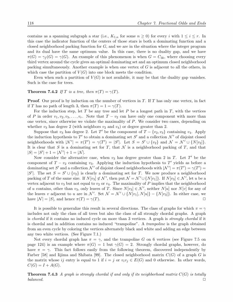
118 Chapter 7. Fractional Odds and Ends
contains as a spanning subgraph a star (i.e., K1,n for some n ≥ 0) for every i with 1 ≤ i ≤ r. Inthis case the indicator function of the centers of those stars is both a dominating function and aclosed neighborhood packing function for G, and we are in the situation where the integer programand its dual have the same optimum value. In this case, there is no duality gap, and we haveπ(G) = γf (G) = γ(G). An example of this phenomenon is when G = C3k, where choosing everythird vertex around the cycle gives an optimal dominating set and an optimum closed neighborhoodpacking simultaneously. Another example is when one vertex of G is adjacent to all the others, inwhich case the partition of V (G) into one block meets the condition.
Even when such a partition of V (G) is not available, it may be that the duality gap vanishes.Such is the case for trees.
Theorem 7.4.2 If T is a tree, then π(T ) = γ(T ).
Proof. Our proof is by induction on the number of vertices in T . If T has only one vertex, in factif T has no path of length 3, then π(T ) = 1 = γ(T ).
For the induction step, let T be any tree and let P be a longest path in T , with the verticesof P in order v1, v2, v3, . . . , vr. Note that T − v2 can have only one component with more thanone vertex, since otherwise we violate the maximality of P . We consider two cases, depending onwhether v3 has degree 2 (with neighbors v2 and v4) or degree greater than 2.
Suppose that v3 has degree 2. Let T ′ be the component of T − {v2, v3} containing v4. Applythe induction hypothesis to T ′ to obtain a dominating set S′ and a collection N ′ of disjoint closedneighborhoods with |N ′| = π(T ′) = γ(T ′) = |S′|. Let S = S′ ∪ {v2} and N = N ′ ∪ {N [v2]}.It is clear that S is a dominating set for T , that N is a neighborhood packing of T , and that|S| = |S′|+ 1 = |N ′|+ 1 = |N |.
Now consider the alternative case, when v3 has degree greater than 2 in T . Let T ′ be thecomponent of T − v2 containing v3. Applying the induction hypothesis to T ′ yields as before adominating set S′ and a collection N ′ of disjoint closed neighborhoods with |N ′| = π(T ′) = γ(T ′) =|S′|. The set S = S′ ∪ {v2} is clearly a dominating set for T . We now produce a neighborhoodpacking of T of the same size. If N [v3] �∈ N ′, then put N = N ′∪{N [v1]}. If N [v3] ∈ N ′, let u be avertex adjacent to v3 but not equal to v2 or v4. The maximality of P implies that the neighborhoodof u contains, other than v3, only leaves of T . Since N [v3] ∈ N ′, neither N [u] nor N [v] for any ofthe leaves v adjacent to u are in N ′. Set N = N ′ ∪ {N [v1], N [u]} − {N [v3]}. In either case, wehave |N | = |S|, and hence π(T ) = γ(T ). �
It is possible to generalize this result in several directions. The class of graphs for which π = γincludes not only the class of all trees but also the class of all strongly chordal graphs. A graphis chordal if it contains no induced cycle on more than 3 vertices. A graph is strongly chordal if itis chordal and in addition contains no induced “trampoline”. A trampoline is the graph obtainedfrom an even cycle by coloring the vertices alternately black and white and adding an edge betweenany two white vertices. (See Figure 7.1.)
Not every chordal graph has π = γ, and the trampoline G on 6 vertices (see Figure 7.5 onpage 124) is an example where π(G) = 1 but γ(G) = 2. Strongly chordal graphs, however, dohave π = γ. This fact follows easily from the following theorem, discovered independently byFarber [58] and Iijima and Shibata [99]. The closed neighborhood matrix C(G) of a graph G isthe matrix whose ij entry is equal to 1 if i = j or vivj ∈ E(G) and 0 otherwise. In other words,C(G) = I +A(G).
Theorem 7.4.3 A graph is strongly chordal if and only if its neighborhood matrix C(G) is totallybalanced. �

7.4 Fractional domination 119
Figure 7.1. The trampoline on 10 vertices.
Theorem 7.4.4 If G is strongly chordal, then π(G) = γ(G).
Proof. The integer program that computes γ(G) is minx · 1 subject to C(G)x ≥ 1. By Theorem7.4.3, C(G) is totally balanced. An appeal to Theorem A.3.4 on page 136 then gives the result. �
A tree is certainly strongly chordal, so Theorem 7.4.2 follows from Theorem 7.4.4.The situation for the total domination number is similar. In this case we replace the notion of
a strongly chordal graph by the notion of a chordal bipartite graph. A graph is chordal bipartiteif it is bipartite and every cycle of length greater than 4 has a chord. Note that chordal bipartitegraphs are not in general chordal.
The total domination number is computed by the integer program minx·1 subject to A(G)x ≥ 1,where A(G) is the usual adjacency matrix of G. The following theorem is due to Hoffman, Kolen,and Sakarovitch [93].
Theorem 7.4.5 A graph is chordal bipartite if and only if A(G) is totally balanced. �
The next theorem follows in the same way as Theorem 7.4.4 above.
Theorem 7.4.6 If G is chordal bipartite, then Π(G) = Γ(G). �
Trees are chordal bipartite, so we obtain the following analogue to Theorem 7.4.2.
Corollary 7.4.7 If T is a tree, then Π(T ) = Γ(T ). �
The example of the cycles shows that the converses of most of the results in this section fail.Although C6 is not strongly chordal, π(C6) = 2 = γ(C6). Although C8 is not chordal bipartite,Π(C8) = 4 = Γ(C8). It seems to be a difficult problem to characterize those graphs for which π = γor Π = Γ.
Even when the duality gap does not vanish, i.e., when π < γ, it is possible for γf to equal eitherγ or π. The simplest example known where π < γf = γ is the graph G pictured in Figure 7.2, dueto Fisher [64].
A simple example where π = γf < γ is the graph pictured in Figure 7.3.We leave it as an exercise to compute the closed neighborhood packing number, the domination
number, and the fractional domination number of these examples to demonstrate that they areindeed examples illustrating what we claim. (See exercises 7–9 on page 128.)
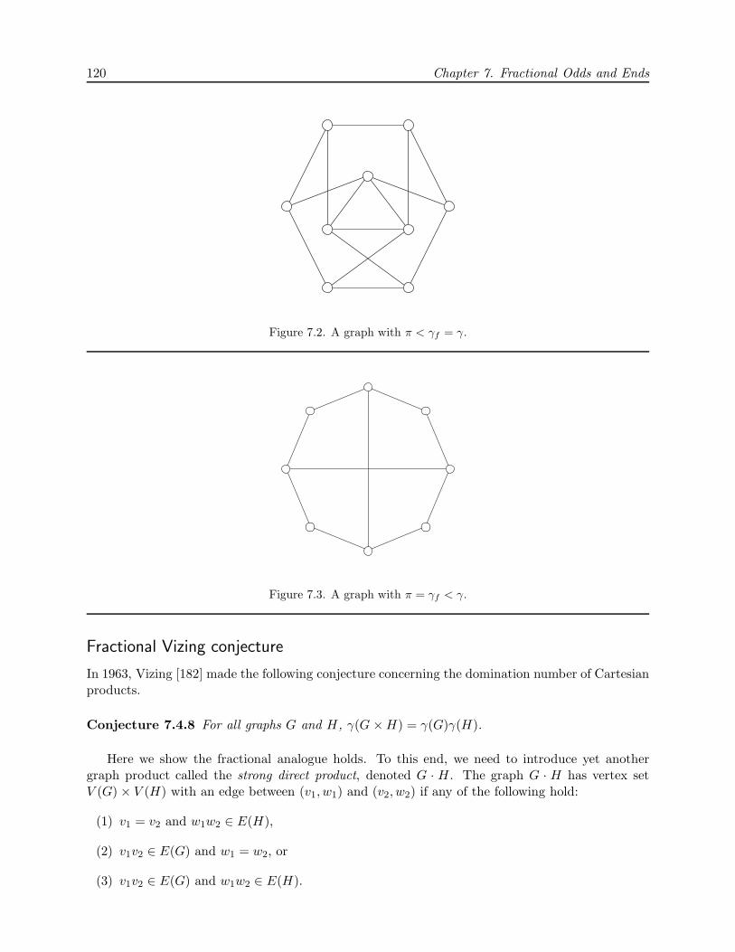
120 Chapter 7. Fractional Odds and Ends
Figure 7.2. A graph with π < γf = γ.
Figure 7.3. A graph with π = γf < γ.
Fractional Vizing conjecture
In 1963, Vizing [182] made the following conjecture concerning the domination number of Cartesianproducts.
Conjecture 7.4.8 For all graphs G and H, γ(G ×H) = γ(G)γ(H).
Here we show the fractional analogue holds. To this end, we need to introduce yet anothergraph product called the strong direct product, denoted G · H. The graph G · H has vertex setV (G) × V (H) with an edge between (v1, w1) and (v2, w2) if any of the following hold:
(1) v1 = v2 and w1w2 ∈ E(H),
(2) v1v2 ∈ E(G) and w1 = w2, or
(3) v1v2 ∈ E(G) and w1w2 ∈ E(H).

7.5 Fractional intersection number 121
The Cartesian product G×H is the spanning subgraph of the strong direct product G·H consistingof edges of type (1) and (2).
The strong direct product is a natural one in the study of domination, because dominating setslift naturally to this product. To be precise, if S ⊆ V (G) is a dominating set for G and T ⊆ V (H)is a dominating set for H, then S × T is a dominating set for G ·H. (Note that the same assertioncannot be made about the Cartesian product G×H.) It follows that
γ(G ·H) ≤ γ(G)γ(H) (7.1)
Alsoγ(G ·H) ≤ γ(G×H), (7.2)
since removing edges from a graph cannot make it easier to dominate. Vizing’s conjecture assertsthat inequality (7.1) is stronger than inequality (7.2).
The fractional analogue of Vizing’s conjecture follows from LP-duality.
Theorem 7.4.9 For all graphs G and H, γf (G×H) ≥ γf (G)γf (H).
Proof. If f is a dominating function for G and g is a dominating function for H, then the “productlifting” defined by h(v,w) = f(v)g(w) is easily seen to be a dominating function for G · H. If fand g are further assumed to be optimal, then the total weight of h is∑
(v,w)∈V (G·H)
h(v,w) =∑
v∈V (G)
∑w∈V (H)
f(v)g(w) = γf (G)γf (H).
We therefore obtain γf (G ·H) ≤ γf (G)γf (H), the fractional analogue of inequality (7.1).The opposite inequality comes from duality. If f is now taken to be a closed neighborhood
packing function for G and g is taken to be a closed neighborhood packing function for H, thenh(v,w) = f(v)g(w) is a closed neighborhood packing function for G ·H. This allows us to obtainan inequality for the fractional closed neighborhood packing number of G · H exactly as in theprevious paragraph, but (critically) with the inequality reversed, since the closed neighborhoodpacking number is a maximization parameter. By LP-duality, this gives γf (G ·H) ≥ γf (G)γf (H).
Hence γf (G ·H) = γf (G)γf (H). Since the fractional analogue of inequality (7.2), namely thatγf (G ·H) ≤ γf (G×H), follows again from the simple fact that G×H is a subgraph of G ·H, weobtain our result. �
7.5 Fractional intersection number
An intersection representation of a graph G = (V,E) is an assignment of a set Sv to each vertexv ∈ V so that uv ∈ E if and only if Su ∩ Sv �= ∅. It is not hard to see that every graph has anintersection representation: Let Sv be the set of edges incident at v.
We have made no assumption on the structure of the sets Sv. If, however, we require that thesets Sv be intervals on the real line, then not all graphs admit such interval representations. Forexample, C4 cannot be represented as the intersection graph of real intervals. The intersectiongraphs of real intervals are known as interval graphs.
In this section, we consider intersection representations by finite sets. In this case, we define thesize of an intersection representation v �→ Sv to be the cardinality of the union of the sets assignedto vertices, i.e., ∣∣∣∣∣
⋃v∈V
Sv
∣∣∣∣∣ .

122 Chapter 7. Fractional Odds and Ends
The intersection number of G, denoted I(G), is the smallest size of an intersection representationof G. Clearly, I(G) ≤ ε(G).
Alternatively, we can express I(G) as a covering number. Define a hypergraph H whose verticesare the edges of G and whose hyperedges correspond to the cliques of G, that is, given a clique of G,the edges induced by that clique form a hyperedge of H. One checks that k(H) = I(G) (exercise 16on page 129).
Proposition 7.5.1 The intersection number of a graph is the size of a smallest covering of theedges of the graph by cliques. �
Thus, it is natural to define the fractional intersection number If (G) to be kf (H).The fractional intersection number completes a “triangle” with the fractional chromatic and
matching numbers. The fractional matching number can be cast as a covering problem involvingvertices and edges. The fractional chromatic number can be cast as a covering problem involvingvertices and cliques.1 Thus we have studied vertex-edge and vertex-clique covering problems andthe “triangle” is completed by considering edge-clique covering problems, i.e., intersection number.
In this section we explore the gap between I(G) and If (G) considering first instances wherethese invariants are the same, and then, instances where they are wildly different.
In case G is a bipartite or, more generally, a triangle-free graph, the only cliques in G are theedges of G. Thus I(G) = If (G) = ε(G). We show that equality also holds for interval graphs and,more generally, chordal graphs. Recall that a graph is called chordal provided it does not containCk with k ≥ 4 as an induced subgraph. In a sense, chordal graphs are generalizations of trees:trees have no cycles, whereas chordal graphs have no chordless cycles. Analogous to leaves in trees,chordal graphs have simplicial vertices: vertices whose neighborhoods are cliques.
Theorem 7.5.2 Every chordal graph has a simplicial vertex. �
We use the above result to prove the following.
Theorem 7.5.3 Let G be a chordal graph. Then I(G) = If (G).
Proof. The packing problem dual to intersection number is to find the maximum number of edgesin G no two of which are in the same clique. Here we present an algorithm that simultaneouslyconstructs a cover of E(G) by cliques and a packing of edges into cliques, and the covering andpacking have the same size. In other words, we show that p(H) = k(H) where H is the edge-cliqueincidence hypergraph of G.
Consider the following algorithm that takes as input a chordal graph G. During the course ofthis computation, we keep track of the “weight” of edges (either 0 or 1), the “weight” of variouscliques (again, 0 or 1), and a label on each edge (either “covered” or “uncovered”).
1. Initialize by setting all edge and clique weights to 0, and marking all edges “uncovered”. LetG1 = G.
2. FOR i = 1 to |V (G)| − 1 DO:
(a) Let vi be a simplicial vertex of Gi, and let Si be the clique consisting of vi and all itsneighbors in Gi.
1More properly, fractional chromatic number is a covering problem involving vertices and independent sets (notcliques), but the chromatic number of the complement of a graph deals with vertex-clique covering.

7.5 Fractional intersection number 123
(b) IF some edge of Gi incident with vi is marked “uncovered” THEN:
• Let clique Si have weight 1.• Select an edge incident with vi that is marked “uncovered” and assign it weight 1.• Mark all edges induced by Si “covered”.
(c) Let Gi+1 = Gi − vi.
3. Output the sum of the weights of the edges of G.
To complete the proof, one notices that at every step of the FOR loop the total weight on theedges equals the total weight on the cliques. Further, by the end of the algorithm every edge ismarked “covered” and is, indeed, covered by some clique Si that was given weight 1. Thus theset of cliques with weight 1 gives a covering of E(G). Finally, one checks that no clique of G cancontain two edges of weight 1 (since covered edges are never selected) and therefore edges of weight1 form a packing of edges into the cliques of G. Thus the sum of the edge weights k(H) equals thesum of the vertex weights p(H). �
Interval graphs form a subfamily of chordal graphs, so, naturally, it follows from Theorem 7.5.3that I = If for interval graphs. However, a bit more can be said.
Theorem 7.5.4 If G is an interval graph, then If (G) = I(G). Moreover, if G has no isolatedvertices, then I(G) equals the number of maximal cliques in G.
To prove Theorem 7.5.4 we use the following result due to Helly [88].
Theorem 7.5.5 If a collection of real intervals has nonempty pairwise intersection, then the in-tersection of all the intervals in the family is nonempty.
Proof. Exercise 18 on page 129. �
Proof (of Theorem 7.5.4). Let G be an interval graph with M maximal cliques. Since every edgeis in some maximal clique, we have If (G) ≤ I(G) ≤ M . Thus, it is enough to show M ≤ If (G).To this end, fix an interval representation of G in which the endpoints of all intervals are distinct;let Iv denote the interval assigned to v ∈ V (G).
Let S be a maximal clique of G. By the Helly property (Theorem 7.5.5), the intersection of allintervals assigned to vertices in S is nonempty, and is therefore an interval, which we denote JS .Note that JS is either (a) an interval assigned to a vertex x, i.e., JS = Ix, or (b) the intersection ofexactly two intervals assigned to vertices x and y, i.e., JS = Ix∩ Iy. See Figure 7.4 on the followingpage. We choose an edge eS depending on which of these cases, (a) or (b), occurs. In case (a) leteS be any edge incident with x, and in case (b) let eS = xy.
The map S �→ eS selects exactly one edge in each maximal clique. Further, the only maximalclique that can contain eS is S because if eS were in some other clique T , then JS and JT wouldintersect, implying that S ∪ T is also a clique, and thereby contradicting the maximality of S andT . Thus the assignment S �→ eS is one-to-one and every clique of G contains at most one selectededge. Thus the selected edges form a packing of edges into cliques, and therefore
M = p(H) ≥ pf (H) = If (G)
where H is the edge-clique hypergraph of G. �

124 Chapter 7. Fractional Odds and Ends
Figure 7.4. The intersection of pairwise intersecting intervals is either (a) one of the original intervals, or(b) the intersection of exactly two of the intervals.
Figure 7.5. A chordal graph for which I = If = 3, but that has 4 maximal cliques.
Note that the stronger conclusion of Theorem 7.5.4 does not apply to chordal graphs: Figure 7.5presents a chordal graph with I = If = 3 but that has 4 maximal cliques.
Theorems 7.5.3 and 7.5.4 describe situations in which intersection number and fractional inter-section number are equal. One might ask: How different can these invariants be? The answer is:Very.
Theorem 7.5.6 Let G = K(n1, n2, . . . , np) be a complete multipartite graph with part sizes n1 ≥n2 ≥ · · · ≥ np. Then If (G) = n1n2.
Proof. Let the jth part of G be Aj with |Aj | = nj. The maximal cliques of G are formed byselecting one vertex from each of the p parts. We form a fractional intersection representation ofG by assigning weight 1/(n3n4 · · · np) to every maximal clique. Note that an edge between parts iand j is in exactly (
∏nk)/(ninj) maximal cliques and receives total weight
n1n2
ninj≥ 1.
Thus this weighting is a feasible fractional edge cover by cliques. Furthermore, the sum of theweights on all cliques is precisely n1n2 and therefore If (G) ≤ n1n2.
On the other hand, if we weight the edges between parts A1 and A2 with weight exactly 1 and allother edges with weight 0, then every clique contains total weight at most 1. This edge weighting istherefore feasible for the dual problem and uses total weight equal to n1n2. Thus If (G) ≥ n1n2. �

7.6 Fractional dimension of a poset 125
Theorem 7.5.6 on the facing page implies that the fractional intersection number of the gener-alized octahedron graph K(2, 2, 2, . . . , 2) is exactly 4. However, we show next that the intersectionnumber of this graph goes to infinity as the number of parts increases.
Theorem 7.5.7 Let n be a positive integer and let G = K(2, 2, . . . , 2) be the complete multipartitegraph with n parts of size 2. Then I(G) ∼ lg n.
Proof. Label the vertices of G as x1, y1, x2, y2, . . . , xn, yn with xi �∼ yi.Let U = {1, 2, . . . , 2t} and construct an intersection representation of G in which each vertex
of G is assigned a t-element subset of U . Note that there are(2t
t
)possible sets, so we take t just
large enough that(2t
t
) ≥ 2n. This gives 2t = (1 + o(1)) lg n. The assignment is now quite simple.Having chosen sets for x1, y1, . . . , xi, yi, we assign to xi+1 any as yet unassigned t-set of U and weassign to yi+1 its complement. With this assignment, any two sets intersect unless they correspondto a pair xi, yi. Thus we have I(G) ≤ 2t = (1 + o(1)) lg n.
For the lower bound, fix an intersection representation of G of smallest size and let I(G) = k.We may assume that the representation chooses its subsets from [k] = {1, . . . , k}. Note that notwo vertices are assigned the same set (otherwise we would have a pair of adjacent vertices withidentical neighbor sets). Thus 2k ≥ 2n because all 2n vertices must receive distinct subsets of [k].Thus I(G) = k ≥ lg n. �
7.6 Fractional dimension of a poset
In this section, we leave graph theory to illustrate how the fractional paradigm can be applied inanother part of combinatorics.
A partially ordered set (or poset for short) is a pair P = (X,≤) where X is a finite set, calledthe ground set of P , and ≤ is a relation on X that satisfies
• (reflexivity) ∀x ∈ X, x ≤ x;• (antisymmetry) ∀x, y ∈ X, (x ≤ y and y ≤ x)⇒ x = y; and
• (transitivity) ∀x, y, z ∈ X, (x ≤ y and y ≤ z)⇒ x ≤ z.We write x < y if x ≤ y and x �= y. Further, we write x ≥ y or x > y provided y ≤ x or y < xrespectively. If either x ≤ y or y ≤ x we say x and y are comparable; otherwise, x and y areincomparable. A subset C of X is called a chain provided any two elements in C are comparable.A subset A of X is called an antichain provided any two distinct elements in A are incomparable.
A partially ordered set P = (X,≤) is called a linear or total order if any two elements in theground set X are comparable, in other words, if the entire ground set X is a chain.
Let P = (X,≤) be a partially ordered set and let L = (X,≤′) be a partially ordered set on thesame ground set. We say that L is a linear extension of P provided (1) L is a linear order, and(2) if x ≤ y (in P ) then x ≤′ y (in L).
A realizer for a poset P is a family R = {L1, L2, . . . , Lt} of linear extensions of P with theproperty that, for all x, y ∈ X, we have x ≤ y in P if and only if x ≤ y in every Li.
The dimension of a poset P , denoted dimP , is the smallest size of a realizer.The dimension of a partially ordered set can be arbitrarily large. The following poset, denoted
Sn, is a standard example. Let n ≥ 2 be an integer. The ground set of Sn is {a1, a2, . . . , an, b1, b2, . . . , bn}.The order relation of Sn can be described as follows. The a’s are pairwise incomparable, as arethe b’s. The only strict relations are those of the form ai < bj with i �= j. See Figure 7.6. Thedimension of Sn is n; see exercise 14 on page 129.

126 Chapter 7. Fractional Odds and Ends
Figure 7.6. The poset S4 has dimension 4 and fractional dimension 4.
The dimension of a poset can be described as the covering number of a hypergraph H. LetP = (X,≤) be a poset, and let L be the set of all linear extensions of P . The vertices of H are allthe ordered pairs (x, y) with x and y incomparable. The hyperedges of H correspond to the linearextensions of P . For L ∈ L, let EL consist of those ordered pairs (x, y) for which x < y in L. Onechecks that dimP = k(H).
The fractional dimension of P , denoted dimfP , can therefore be defined as kf (H). We canalso define the fractional dimension as follows. Let t be a positive integer. A t-fold realizer ofP = (X,≤) is a multiset Rt = {L1, . . . , Lm} of linear extensions of P with the property that, forall x, y ∈ X with x and y incomparable, there are at least t linear orders in Rt for which x < y andat least t for which x > y. We also call t-fold realizers multirealizers.
Let dimt(P ) denote the smallest size of a t-fold realizer. Then dimfP = limt→∞(dimt P )/t.For example, the fractional dimension of the standard example Sn is n; see exercise 14.
Let P = (X,≤) and let x ∈ X. The degree of x is the number of other elements in X to whichx is comparable. We can bound the dimension of a poset in terms of its maximum degree.
Theorem 7.6.1 Let P be a poset with maximum degree d. Then dimP ≤ 50d log2 d. �
For fractional dimension, the following holds.
Theorem 7.6.2 Let P be a poset with maximum degree d. If P is not an antichain, then dimf P ≤d+ 1. �
Moreover, the standard example Sn has maximum degree n − 1 and fractional dimension n,showing that the bound in Theorem 7.6.2 is the best possible.
Can dimension and fractional dimension be very different? The answer is yes. An intervalorder is a partially ordered set arising from the left-to-right order of intervals on the real line. Moreprecisely, we say P = (X,≤) is an interval order provided we can assign to each x ∈ X a realinterval Ix so that x < y in P if and only if Ix is completely to the left of Iy. Interval orders canhave arbitrarily high dimension.
Theorem 7.6.3 Let k be a positive integer. Then there exists an interval order P with dimP =k. �
By contrast, however, every interval order has small fractional dimension.
Theorem 7.6.4 Let P be an interval order. Then dimfP < 4.
To prove this, we need the following fact about interval orders.

7.7 Sperner’s theorem: a fractional perspective 127
Theorem 7.6.5 Let P = (X,≤) be an interval order. Then for every partition X = A ∪ B thereexists a linear extension L = (X,≤′) of P with the property that for all a ∈ A and b ∈ B with a �> bwe have a <′ b. �
Informally stated, Theorem 7.6.5 asserts that for any partition A ∪ B of the ground set of aninterval order P we can make a linear extension in which all the elements in A are below all theelements in B, except when an element of A is above an element of B in P .
Proof (of Theorem 7.6.4). Let P = (X,≤) be an interval order and let |X| = 2n. (We maysuppose |X| is even. If not, we may add another element to P that is below all the others. Thisaugmented poset is also an interval order and its fractional dimension is at least that of P .) Webuild a multirealizer for P as follows. Let A ∪ B be a partition of X with |A| = |B| = n. LetLA be a linear extension of P as described in Theorem 7.6.5. Let R be the multiset of all linearextensions LA, as A varies over the subsets of X with n elements. For every incomparable pair ofelements (x, y), there are at least
(2n−2n−1
)members of R in which x < y. Also, |R| = (2n
n
), hence
dimfP ≤(2n
n
)(2n−2
n−1
) =2n(2n− 1)
n2< 4. �
Recently, Trotter and Winkler [179] have shown that the upper bound of 4 in Theorem 7.6.4 istight.
7.7 Sperner’s theorem: a fractional perspective
Let P = (X,≤) be a poset. A chain in P is a subset C ⊆ X in which any two elements arecomparable. Similarly, an antichain is a subset A ⊆ X in which any two distinct elements areincomparable. The height of P is the maximum size of a chain in P and the width of P is themaximum size of an antichain.
Another way to express these ideas is to consider the comparability graph of P : Let G(P ) bethe graph whose vertex set is X with an edge joining x and y just when x < y or y < x. Then achain in P is simply a clique in G(P ) and an antichain in P is an independent set. The height andwidth of P are just the clique and independence number of G(P ).
We may define the fractional height and width of a poset to be the fractional clique and inde-pendence numbers of the comparability graph of the poset. However, because comparability graphsare perfect, fractional height and width reduce to their integer counterparts. Indeed, the equalityα(G(P )) = χ(G(P )) is a restatement of the following result of Dilworth [43].
Theorem 7.7.1 (Dilworth) The width of a poset equals the minimum size of a partition of theposet into chains. �
Although the notions of fractional height and width yield nothing new, the fractional approachis helpful in considering the following classical problem.
Let [n] = {1, 2, . . . , n} and let 2[n] denote the poset of all subsets of [n] ordered by containment.The height of this poset is clearly n+1, but what of its width? Note that for each k with 0 ≤ k ≤ n,the subsets of [n] of cardinality k form an antichain of size
(nk
). The largest antichain of this sort
has size( n�n/2�
). Can a larger antichain be found? The answer is no [170].
Theorem 7.7.2 (Sperner) The width of 2[n] is( n�n/2�
).

128 Chapter 7. Fractional Odds and Ends
Proof. Form a hypergraph H whose vertices are the 2n subsets of [n] and whose hyperedges arethe maximal chains in 2[n], i.e., the chains of size n + 1. The width of 2[n] is exactly the coveringnumber k(H), which by Dilworth’s theorem equals kf (H). Note that H is edge-transitive (allmaximal chains in 2[n] look the same) so in a fractional covering of H we may assign all n! of themthe same weight w without loss of optimality. (See Proposition 1.3.4 on page 5 and exercise 4 onpage 12.) Choose A ∈ 2[n] with |A| = a. The total weight of all chains containing A is wa!(n− a)!.The least w that gives a feasible fractional cover satisfies
w
⌊n
2
⌋!⌈n
2
⌉! = 1,
which gives
kf (H) = n!w =n!⌊
n2
⌋!⌈
n2
⌉!
=
(n
�n/2�
). �
7.8 Exercises
1. Let H be the hypergraph whose vertices are the edges of a graph G and whose hyperedgescorrespond to the graph’s planar subgraphs. Thus θ(G) = k(H). Show by example that Hneed not be a matroid.
2. Prove that for all n ≥ 3 we have θ(Kn) = �θf (Kn)� except for n = 9, 10.
3. Prove that if a graph has an Eulerian tour then it must have a cycle double cover.
4. Let k be a positive integer and let G be a graph. Call a family of cycles of a graph G a cyclek-fold cover if every edge of G is in exactly k of the given cycles.
Prove that if k is odd, then G has a cycle k-fold cover iff G is Eulerian.
5. Show that for x ≥ 2 we have rf (x, 2) = x.
6. The fractional Ramsey number rf (x, y) as we have defined it is obviously integer-valued. Hereis another way to fractionalize the Ramsey number.
The notation n −→ (a, b) means that for any partition E(Kn) = A ∪B there must be eithera Ka on the A-edges or a Kb on the B-edges. Now r(a, b) is the least n for which n −→ (a, b)is true.
Fractionalize this by defining z∗−→ (x, y) to mean that if G = (V,E) is any graph with
ωf (G) ≥ z, then for any partition E = A ∪ B we have either ωf (V,A) ≥ x or ωf (V,B) ≥ y.Let r∗(x, y) be the infimum of all z for which z ∗−→ (x, y) is true.
Prove that if x, y > 2 then r∗(x, y) = xy.
7. Compute π, γf , and γ for the icosahedron and the dodecahedron.
8. Compute π, γf , and γ for the graphs in Figures 7.2 and 7.3.
9. Show that no inequality holds between γ(G) and Γf (G) by finding two graphs G and H withγ(G) < Γf (G) and with γ(H) > Γf (H).
10. Show that Γf (G) = 1 if and only if Δ(G) = n− 1.

7.9 Notes 129
11. Generalize Theorem 7.4.1 on page 117 by showing that, for any graph G, n/(1 + Δ(G)) ≤γf (G) ≤ n/(1 + δ(G)) and n/Δ(G) ≤ Γf (G) ≤ n/δ(G).
12. Find the domination number and the fractional domination number of the path Pn, the 2×ngrid Pn × P2, and the 3× n grid Pn × P3.
13. A block in a graph is a maximal 2-connected subgraph. A block graph is a graph every one ofwhose blocks is complete. Show that π(G) = γ(G) for every block graph G.
14. For n ≥ 2 show that dimSn = dimfSn = n, where Sn is the standard example defined onpage 125.
15. Prove Theorem 7.6.2 on page 126 in the special case that P has height 2. (The height of aposet is the maximum cardinality of a chain.)
Hint: Suppose there are n minimal elements. Build a multirealizer by taking all n! linearorders on the minimal elements and place the maximal elements into these linear orders aslow as possible.
16. Prove that the intersection number of a graph equals the covering number of the edge-cliqueincidence hypergraph of the graph.
17. A graph G is called cobipartite provided its complement, G, is bipartite. It is called locallycobipartite if for every vertex v the subgraph of G induced by the neighbors of v, i.e., G[N(v)],is cobipartite.
It is conjectured that if a graph is locally cobipartite then I(G) ≤ ν(G). Prove the fractionalversion of this conjecture, i.e., if G is locally cobipartite, then If (G) ≤ ν(G).
18. Prove Theorem 7.5.5 on page 123.
7.9 Notes
For an introduction to topological graph theory see Gross and Tucker [80], Mohar and Thomassen[133], Thomassen [176], or White and Beineke [188]. Theorem 7.1.1 on page 111 is a consequenceof a result of Battle, Harary, Kodama, and Youngs [11]. Theorem 7.1.2 is from [173] by Stahl andBeineke. The history of Theorem 7.1.6 on page 113 is recounted in Thomassen [176], and in Whiteand Beineke [188]. The result is based largely on the work of Beineke and Harary [21].
The Cycle Double Cover Conjecture 7.2.1 on page 113 was first posed by Szekeres in 1973 andindependently by Seymour in 1979. Genghua Fan [57] has shown that every 2-edge-connected graphadmits a cycle sextuple cover, i.e., a family of cycles that includes each edge of G exactly 6 times.Together with Jaeger’s [101] result, this means that every 2-edge-connected graph admits a cyclek-fold cover for all even k ≥ 4. In case k is odd, a graph has a cycle k-fold cover if and only if it isEulerian. (See exercise 4.) Thus only the case k = 2 is open.
Paul Seymour [163] has proved a theorem on fractional directed cycle packing that is the frac-tional analogue of a conjecture of Younger. Recently, Reed, Robertson, Seymour, and Thomas [153]have proved this conjecture.
Theorem 7.3.1 and exercise 6 are from Jacobson, Levin, and Scheinerman [120], which also givespartial results on the more-than-two-color case. In particular, if k ≥ 2 is an integer, one has
rf (k, k, . . . , k) =kp+1 − 2kp + k
k − 1

130 Chapter 7. Fractional Odds and Ends
where p is the number of k’s.The fractional domination number was first encountered in a paper by Farber [58]. There is by
now an extensive body of literature on domination, its relatives, and their fractional counterparts;see the paper [111] by Domke, Fricke, Laskar, and Majumdar for an overview of these results.Surveyed there are results not only on the domination number and the total domination number, butalso on an assortment of other parameters known as the upper domination number, the independentdomination number, the irredundance number, and the upper irredundance number, all of whichcan be fractionalized. Theorem 7.4.1 on page 117 was first noticed by Domke [44]. Theorem 7.4.2on page 118 is due to Meir and Moon [131]. Theorem 7.4.9 on page 121 is due to Fisher, Ryan,Domke, and Majumdar [67].
It is an open problem to characterize those graphs G every one of whose maximal indepen-dent sets contains α(G) elements. A fractional analogue is addressed in a paper by Currie andNowakowski [41], where there appears a characterization of those graphs every one of whose mini-mal dominating functions attains the fractional domination number. For such graphs, the fractionaldomination number can be computed in a greedy way: Begin by assigning weight 1 to every vertexand then simply decrease the weights on vertices (taking the vertices in any order at all) makingcertain to maintain a weight of at least one on every closed neighborhood. When the last vertex isreached, the sum of all the weights will be γf (G).
The material on fractional intersection number is due to Scheinerman and Trenk [159]. Exer-cise 17 on the preceding page, due to Chi Wang, is a weakened version of a conjecture of Opsut [140].
For an all-encompassing introduction to dimension theory for partially ordered sets, see Trotter’sbook [178]. Theorem 7.6.1 is due to Furedi and Kahn [72]. The log-squared term in this bound mightnot be best possible, but can’t be replaced by anything less than a log term; see Erdos, Kierstead,and Trotter [54]. The results on fractional dimension are from Brightwell and Scheinerman [30],and Felsner and Trotter [61]. Theorem 7.6.2 can be improved by defining the up-degree and down-degree of x to be the number of elements strictly greater than x and less than x, respectively. LetΔU and ΔD be the maximum up and down degrees of a poset. Then Felsner and Trotter [61] showthat dimfP ≤ 1 + min {ΔU(P ),ΔD(P )}.
For more information about interval orders and graphs, see Fishburn’s book [62]. Theorem 7.6.3on page 126 is due to Bogart, Rabinovitch, and Trotter [22]; see also Furedi, Hajnal, Rodl andTrotter [71]. Theorem 7.6.5 is from a paper by Rabinovitch [149].
The proof we present of Sperner’s theorem 7.7.2 on page 127 is a fractionalized version ofLubell’s proof in [125]. See also the monograph [7] by Anderson.

Appendix A
Background
This appendix has two purposes: to record basic notation (especially in graph theory) and to givea brief introduction to mathematical programming and subadditivity.
We assume our reader has a basic grounding in discrete mathematics, especially in graph theory.Because graph theory is a relatively young discipline, its notations are not 100% standardized. Herewe simply list basic notation used in this book. Fundamental graph theory definitions are not alwaysgiven; the reader should consult a text such as Berge [15], Bondy and Murty [26], Chartrand andLesniak [35], Harary [83], or West [187].
We also give a brief introduction to linear (and integer) programming. Readers not familiarwith basic LP theory (especially duality) should read this section before beginning to read the text.For a more thorough introduction, see a text such as Chvatal [38] or Schrijver [160].
The subadditivity lemma from analysis is developed in §A.4. Again, readers not conversantwith this tool should read this section carefully before beginning the main portion of this book.
A.1 Basic graph theory and notation
A graph is a pair G = (V,E) where V is a finite set and E is a set of 2-element subsets of V . Thus,for us, a graph is what is commonly called a simple graph, i.e., a graph without loops or paralleledges. A multigraph may have loops and parallel edges.
We abbreviate {v,w} ∈ E(G) to vw ∈ E(G) or sometimes v ∼ w. In this case we say that vand w are adjacent. When e = vw, we may write v ∈ e and say that v and e are incident. We useν(G) and ε(G) to denote |V (G)| and |E(G)| respectively.
The following is a list of most of the notation used in this book. When a set of numbersfollows an item, these numbers refer to the pages on which the relevant concepts are introduced ordiscussed.
If a symbol in this book appears with the subscript f , it is the fractional analogue of theunsubscripted symbol.
• α(G): independence number of G.
• A(G): adjacency matrix of G.
• B(G): bipartite split of G. {17, 107}• Cn: cycle on n vertices.
• c(G): number of components of G. {22}• χ(G): chromatic number of G. {30}• χ′(G): edge chromatic number of G. {57}• χ′′(G): total chromatic number of G. {63}
131

132 Appendix
• d(v): degree of a vertex v.
• dk(v): iterated degree sequence of v. {102}• d(v, S): number of edges from v to S. {100}• d(G): average degree in G. {73}• δ(G): minimum degree of a vertex in G.
• Δ(G): maximum degree of a vertex in graph G.
• D(v), D(G): ultimate degree sequence of a vertex v, of a graph G. {102}• ∂v, ∂S, ∂H: set of edges with exactly one end at v, in S, in V (H). {59}• dimP : dimension of poset P . {125}• E(G): edge set of G.
• ε(G): number of edges in G, i.e., |E(G)|.• η: orthonormal representation invariant. {41}• g(G), g(G): genus, nonorientable genus of G. {111}• γ(G), Γ(G): domination number, total domination number of G. {116}• i(G): number of isolated vertices in G. {18}• I(G): intersection number of G. {121}• J : matrix of all ones. {94}• Kn: complete graph on n vertices.
• Kn,m: complete bipartite graph.
• K(n1, n2, . . . , np): complete multipartite graph.
• k(H): covering number of hypergraph H. {1}• κ′(G): edge connectivity of G. {25}• L(G): line graph of G.
• Λ(G): lower bound for edge chromatic number. {58}• M(G), M(H): vertex-edge incidence matrix of graph G, hypergraph H. {1, 15}• M(G): matching polytope of G. {59}• M(G): cycle matroid of G. {74}• M1(G): near acyclic matroid of G. {84}• μ(G), μ(H): matching number of graph G, of hypergraph H. {7, 14}• mad(G): maximum average degree of G. {73}• N(v), N [v]: open, closed neighborhood of vertex v. {116}• ν(G): number of vertices in G, i.e., |V (G)|.• o(G): number of odd components in G. {18}• ω(G): clique number of G.

A.1 Basic graph theory and notation 133
• Pn: path on n vertices.
• p(H): packing number. {2}• π(G): closed neighborhood packing number of G. {116}• Π(G): open neighborhood packing number of G. {116}• Π(v): permutation polytope of vector v. {98}• r(n,m): Ramsey number. {114}• ρ(M), ρ(S): rank of a matroid M, of a set S in a matroid. {75}• σ(G), σ′(G): toughness, edge toughness of G. {23, 89}• τ(H): transversal number.
• T (G): total graph of G. {63}• θ(G): thickness of G. {112}• Θ(G): Shannon capacity of G. {41}• Υ(G): arboricity of G. {72}• V (G), V (H): vertex set of graph G, of hypergraph H.
• x(G): crossing number of G. {112}• Y (G): Mycielski’s construction on graph G. {35}• G: complement of G.
• H∗: hypergraph dual of H. {6}• G, M: dual of a planar graph G, of matroid M. {86, 87}• G[A]: induced subgraph of G on vertex set A.
• [A,B]: set of edges with one end in A and the other end in B.
• G×H: Cartesian product of G and H. {120}• G ∗H: disjunctive product of G and H. {38}• G[H]: lexicographic product of G with H. {35}• G ·H: strong direct product of G and H. {120}• v ⊗w, A⊗B: tensor product of vectors v and w, Kronecker product of matrices A and B.{42, 99}
• G+H: disjoint union of G and H.
• G ∨H, P ∨Q: join of graphs G and H, of partitions P and Q. {54, 20}• A⊕B: direct sum of matrices A and B. {96}• G ∼= H: G is isomorphic to H.
• G ∼=′ H: G is semi-isomorphic to H. {106}• G ≤ H: G is an induced subgraph of H.
• G ⊆ H: G is a subgraph of H.
• 〈S〉: convex hull of a set S.
• P≡: equivalence relation derived from partition P. {100}• [n]: the set {1, 2, . . . , n}.

134 Appendix
A.2 Hypergraphs, multigraphs, multisets, fuzzy sets
A hypergraph H is a pair (S,X ) where S is a finite set and X ⊆ 2S . The sets in the family X arecalled the hyperedges of H. A hypergraph is also known simply as a set system. The rank of ahypergraph is the size of a largest hyperedge. If all members of X are of the same cardinality r,then H is called an r-uniform hypergraph. Graphs are 2-uniform hypergraphs.
A hypergraph H = (S,X ) is called a simplicial complex in case Y ∈ X whenever Y ⊆ X andX ∈ X . If H = (S,X ) is a simplicial complex with at least one edge, then we call H a matroid ifit also satisfies the following condition: for all X,Y ∈ X with |X| > |Y |, there is an x ∈ X − Y sothat Y ∪ {x} ∈ X . (See §5.2.)
A multiset is a pair M = (S,m) where S is a set, called the ground set of M , and m : S → Z+.For an element s in the ground set S the value m(s) is called the multiplicity of s. We think ofm(s) as representing the number of times that s is in M . If x /∈ S we may write m(x) = 0. Thecardinality of M is, naturally, |M | = ∑
s∈S m(s).If M and M ′ are multisets on ground sets S and S′ respectively, their multiset union is M⊕M ′,
the multiset on S ∪ S′ in which the multiplicity of an element s is m(s) +m′(s).When t is a positive integer let t ·M denote the t-fold multiset union M ⊕M ⊕ · · · ⊕M , i.e.,
the multiset in which the multiplicity of an element s is tm(s) where m(s) is its multiplicity in M .We also write t · S where S is a set to denote the multiset whose ground set is S and all of whoseelements have multiplicity equal to t.
A multigraph is a pair G = (V,E) where V is a finite set and E is a multiset of 2-elementmultisets whose ground set is a subset of V . This definition allows for parallel edges (an edge uvwith multiplicity greater than 1) and loops (an edge of the form vv). Although some authors usethe term “graph” to denote what we here call a “multigraph”; we use the term only in the morerestrictive sense.
A fuzzy set is a pair F = (S,w) where S is a set and w : S → (0, 1]. For an element s ∈ S,the value w(s) is called the weight of s. When x �∈ S we may write w(x) = 0. The weight of F isw(F ) =
∑s∈S w(s). It is sometimes convenient to think of w(s) as the “degree of membership” of
the element s in F .Many of the fractional invariants in this book can be defined by taking a definition of a standard
graph invariant verbatim and inserting the word “fuzzy” in an appropriate place. Thus it is oftenappropriate to understand the subscript “f”, which we use throughout to denote a fractionalanalogue, to also stand for the word “fuzzy”.
One can speculate what might be meant by a fuzzy or fractional graph. This could mean a pair(V,E) in which V is a finite set and E is a fuzzy set of 2-element subsets of V . Alternatively, onemight allow V to be a fuzzy set as well. These objects are not considered in this book; we studygraphs and, to the extent that they help us understand graphs, hypergraphs.
A.3 Linear programming
We identify vectors in Rn (n-vectors) with n-by-1 matrices. We write At for the transpose of thematrix A. If A and B are both m-by-n, we write A ≤ B to mean that each entry of A is less thanor equal to the corresponding entry of B. Further, when v is a vector and s is a scalar, we writev ≤ s to mean that every component of v is at most s.
A linear program (LP) is an optimization problem that can be expressed in the form “maximizectx subject to Ax ≤ b”, where b is an m-vector, c is an n-vector, A is an m-by-n matrix, and xvaries over all n-vectors with nonnegative entries. The problem “minimize ctx subject to Ax ≥ b”

A.3 Linear programming 135
is also a linear program; again, we assume that x ≥ 0. It is easy to see that problems with equalityconstraints or with unconstrained variables can be put into the above form, so these variations maybe considered. For our purposes, LPs always take the standard forms introduced here.
An integer program (IP) is an optimization problem of the same form as a linear program exceptthat the vector x is subject to the additional constraint that all its entries must be integers.
In an LP or an IP, the expression ctx is called the objective function, a vector x satisfying theconstraints Ax ≤ b, x ≥ 0 is called a feasible solution, and the optimum of the objective functionover all feasible solutions is called the value of the program. It is natural to assign the value −∞to a maximization program with no feasible solutions and the value +∞ if the objective functionis unbounded on feasible solutions. The linear program obtained from an integer program P bydropping the constraint that the entries of x be integers is called the linear relaxation of P . Amain theme in this book is the connection between integer programs that compute graph-theoreticinvariants and their linear relaxations, which compute the fractional analogues of those invariants.
If P is the (linear or integer) program “maximize ctx subject to Ax ≤ b, x ≥ 0”, then theprogram “minimize bty subject to Aty ≥ c, y ≥ 0” is called the dual of P . If x is a feasible solutionfor P and y is a feasible solution for the dual of P , then, because x,y ≥ 0, we have the weak dualityinequality:
ctx = xtc ≤ xtAty = (Ax)t y ≤ bty. (A.1)
This implies that the value of P is less than or equal to the value of the dual of P . In fact, if P isa linear program, more is true.
Theorem A.3.1 A linear program and its dual have the same value. �
This is a central result in the theory of linear programming and is called the (strong) dualitytheorem. One way to prove it is to analyze an algorithm (the simplex algorithm) that gives afeasible solution x∗ for P and simultaneously a feasible solution y∗ for the dual of P such thatctx∗ = bty∗. This yields the opposite inequality from the one implied by (A.1) and the theoremfollows. For details see any of the many standard books on linear programming.
Not only are the values of an LP and its dual equal, but the vectors achieving this value obeythe complementary slackness condition described in the following result.
Theorem A.3.2 Let x∗ be any optimal solution to the bounded, feasible linear program max ctxsubject to Ax ≤ b, x ≥ 0, and let y∗ be any optimal solution to the dual minbty subject toAty ≥ c, y ≥ 0. Then
x∗ · (Aty∗ − c) = y∗ · (Ax∗ − b) = 0.
Proof. Equality holds in the weak duality condition (A.1) because ctx∗ = bty∗, i.e.,
ctx∗ = (y∗)tAx∗ = (y∗)tb,
from which it follows that(ct − (y∗)tA
)x∗ = 0 and so x∗ ·(Aty∗−c) = 0. We have y∗ ·(Ax∗−b) = 0
by the same reasoning. �
Note that since x∗ and Aty∗−c are nonnegative, Theorem A.3.2 implies that if some coordinateof either x∗ or Aty∗ − c is nonzero, then the corresponding coordinate of the other must be zero.In other words, complementary slackness holds in a term-by-term fashion. The same is true, ofcourse, for y∗ and Ax∗ − b.
136 Appendix
The situation for integer programs is more complicated; the value of an integer program neednot equal the value of its dual. The interval between these two values is called the duality gap. Anynumber in the interior of the duality gap is not achievable as a value of the objective function ofeither the primal program or the dual.
In some situations, the value of an integer program and its linear relaxation are equal. A {0, 1}-matrix M is totally unimodular if detS ∈ {−1, 0, 1} for all square submatrices S (not necessarilyformed from contiguous rows or columns). A {0, 1}-matrix M is (totally) balanced provided noodd-by-odd square submatrix has exactly two ones in every row and column. Note that totalunimodularity implies total balance (exercise 3 on page 138).
The following theorem follows easily from the basic theory of linear programming and fromCramer’s rule for solving linear systems.
Theorem A.3.3 If A,b, c all have integer entries and A is totally unimodular, then the value ofthe integer program “maximize ctx subject to Ax ≤ b,x ≥ 0”, and its linear relaxation are thesame. �
The same conclusion can be drawn from slightly different hypotheses.
Theorem A.3.4 If A,b, c all have integer entries, at least one of b or c is a constant vector, and Ais totally balanced, then the value of the integer program “maximize ctx subject to Ax ≤ b,x ≥ 0”,and its linear relaxation are the same. �
Under the hypotheses of these theorems, the duality gap associated with the IP reduces to asingle point.
Computational complexity
The classic method for finding an optimal solution to a linear program is the simplex algorithm.While this method works reasonably for most problems, it can, in the worst case, take an unrea-sonable amount of time to solve an LP. On the other hand, the ellipsoid algorithm always runsin at most polynomial time, but is not a practical method; on typical problems it is slower thanthe simplex method. Interior point algorithms appear to give us the best of both worlds: goodperformance on typical problems and a polynomial run time in the worst case.
More precisely, we measure the size of an LP as follows. Suppose the LP is
max ctx s.t. Ax ≤ b, x ≥ 0 (A.2)
where A is an m×n matrix. We suppose that the entries in A, b, and c are rational numbers and welet K be the maximum absolute value of the various numerators and denominators of these rationalnumbers when expressed in reduced form. Then the size of the LP is defined to be mn logK. Werewe to input an LP into a computer, the size of the LP is a good measure of how large (how manycharacters long) the input would be. Then when we assert that, say, the ellipsoid algorithm runsin polynomial time, we mean that it runs in time bounded by a polynomial in the size of the LP.
Sometimes the size of an LP is not a fair measure of the size of the problem it is formulated tosolve. For example, consider the LP (Chapter 3) for the fractional chromatic number of a graph. Areasonable measure of the size of an instance of the fractional chromatic number problem of a graphG = (V,E) is |V | + |E|. However, this LP formulation of fractional chromatic number features amatrix whose rows are indexed by V but whose columns are indexed by the independent subsetsof V , and there may be exponentially many (in |V |) independent subsets of V . Indeed, despite

A.4 The subadditivity lemma 137
the fact that linear programs can be solved in polynomial time, the fractional chromatic numberproblem is NP-hard.
Nevertheless, despite the combinatorial explosion inherent in formulating some fractional graphtheory problems as linear programs, a polynomial-time solution (in the size of the graph) may still bepossible. Consider again the LP in equation (A.2) in which the matrix A has m rows and n columnsand the entries in A, b, and c are rational numbers. As before, let K be the maximum absolutevalue of the various numerators and denominators of these rational numbers when expressed inreduced form. Suppose the number of constraints m is exceedingly large compared to the numberof variables n. It would be useful if we could still solve this LP efficiently, i.e., in time polynomialin mn logK. Indeed, this is possible provided there is an efficient (polynomial-time) algorithm forsolving the separation problem:Separation Problem: Given a vector x ≥ 0, decide if x is feasible for the LP, and if not, find aconstraint that is violated.
If we can solve the separation problem efficiently (in time polynomial in n logK) then theellipsoid algorithm can be used to solve the LP in polynomial time.
A.4 The subadditivity lemma
A function g : Z+ → R is called subadditive provided, for all a, b, we have
g(a+ b) ≤ g(a) + g(b).
Lemma A.4.1 (Subadditivity) Suppose g is subadditive and g(n) ≥ 0 for all n. Then the limit
limn→∞
g(n)n
exists and is equal to the infimum of g(n)/n (n ∈ Z+).
Proof. Let x = lim sup g(k)/k and let n be a fixed positive integer. Let m be any (large) integer.Divide m by n and write m = qn + r with 0 ≤ r < n. Note that by subadditivity, g(m) ≤qg(n) + g(r). Dividing by m we have
g(m)m≤ qg(n) + g(r)
qn+ r
≤ qg(n) + g(r)qn
≤ g(n)n
+g(r)qn
.
Choose a sequence of m’s going to infinity so that g(m)/m → x. Note that g(r)qn → 0 since
g(r) is bounded and n is fixed but q → ∞. Thus we have x ≤ g(n)/n for any n. This implieslim inf g(n)/n ≥ x = lim sup g(n)/n, so lim g(n)/n = x and lim g(n)/n = inf g(n)/n. �
We often have use for a multiplicative version of this lemma. A function h : Z+ → R+ is calledsubmultiplicative provided, for all a, b, we have
h(a+ b) ≤ h(a)h(b).

138 Appendix
Lemma A.4.2 Suppose that h is a submultiplicative function with h(n) ≥ 1 for all n. Then thelimit
limn→∞
n
√h(n)
exists and is equal to the infimum of n√h(n).
Proof. Let g(n) = log h(n). Then g(a + b) = log h(a + b) ≤ log h(a)h(b) = log h(a) + log h(b) =g(a) + g(b), so g is subadditive. Lemma A.4.1 then implies that lim g(n)/n = lim log n
√h(n) exists
and equals its infimum. Thus the same is true for lim n√h(n). �
A.5 Exercises
1. Formulate and prove a “superadditivity” lemma.
2. Let g : Z+ → R. Show that if g(a + b + c) + g(c) ≤ g(a + c) + g(b + c) for all a, b, c ∈ Z+,then g(n)/n is a decreasing function of n (hence approaches its limit monotonically).
3. Let M be a 0,1-matrix. Prove that if M is totally unimodular, then M must be totallybalanced.
4. Given a graph G, let A be its adjacency matrix and let b and c be vectors of the appropriatesize all of whose entries are 1. What graph theoretic parameter is given by the value of theLP “maximize ctx subject to Ax ≤ b”?
A.6 Notes
Graph theory is a relatively young discipline, and as such there is not always a single standardfor terminology and notation. We follow mostly the style of Bondy and Murty [26]. Other widelyused introductions to graph theory include Chartrand and Lesniak [35] and Harary [83]. A moresubstantial introduction with a long, excellent list of exercises is West [187].
The theory of hypergraphs is explored in Berge [15] and [19].Linear programming as a discipline goes back to 1947 when George Dantzig invented the simplex
algorithm for solving certain military optimization problems. The proof of the duality theorem isdue to Gale, Kuhn, and Tucker [73], appearing in 1951. A good mathematical treatment of linearprogramming theory is Schrijver [160]. In particular, our Theorem A.3.3 appears there on page 266with proof, and a version of our Theorem A.3.4 appears there on page 305. A gentler introductionto the theory of linear programming is Chvatal [38]. See also Grotschel, Lovasz, and Schrijver [82]or Papadimitriou and Steiglitz [142].
Lemmas A.4.1 and A.4.2 are widely known as folk theorems. They go back to the work ofFekete [60] in 1922.
Bibliography
[1] Aharoni, R., Infinite matching theory, Disc. Math. 95 (1991) 5-22.
[2] Aharoni, R., and R. Ziv, LP duality in infinite hypergraphs, J. Comb. Theory (Ser. B) 50(1990) 82-92.
[3] Alon, N., Restricted colorings of graphs, in Surveys in Combinatorics 1993, K. Walker, ed.,London Mathematical Society Lecture Note Series 187, Cambridge University Press (1993)1-33.
[4] Alon, N., and A. Orlitsky, Repeated communication and Ramsey graphs, IEEE Trans. Info.Theory 41 (1995) 1276-1289.
[5] Alon, N., Z. Tuza, and M. Voigt, Choosability and fractional chromatic numbers, Disc. Math.,to appear.
[6] Andersen, L. D., On edge-colourings of graphs, Math. Scand. 40 (1977) 161-175.
[7] Anderson, I., Combinatorics of Finite Sets, Clarendon Press, Oxford Science Publications(1987).
[8] Balas, E., Integer and fractional matchings, in Studies on Graphs and Discrete Programming,Ann. Disc. Math. 11, P. Hansen, ed., North-Holland (1981) 1-13.
[9] Balinski, M., On the maximum matching, minimum covering, in Proc. Symp. Math. Program-ming, H. W. Kuhn, ed., Princeton University Press (1970) 301-312.
[10] Barany, I., A short proof of Kneser’s conjecture, J. Comb. Theory (Ser. A) 25 (1978) 325-326.
[11] Battle, J., F. Harary, Y. Kodama, and J. W. T. Youngs, Additivity of the genus of a graph,Bull. Amer. Math. Soc. 68 (1962) 565-568.
[12] Behzad, M., Graphs and Their Chromatic Numbers, Ph.D. thesis, Michigan State University(1965).
[13] Behzad, M., The total chromatic number of a graph: a survey, in Combinatorial Mathematicsand its Applications, Academic Press (1971) 1-8.
[14] Berge, C., Sur le couplage maximum d’un graphe, C. R. Acad. Sci. Paris 247 (1958) 258-259.
[15] Berge, C., Graphs and Hypergraphs, North-Holland (1973).
[16] Berge, C., Fractional Graph Theory, ISI Lecture Notes 1, Macmillan of India (1978).
[17] Berge, C., Packing problems and hypergraph theory: A survey, Ann. Disc. Math. 4 (1979)3-37.
[18] Berge, C., Packing problems, in Studies on Graphs and Discrete Programming, Ann. Disc.Math. 11, P. Hansen, ed., North-Holland (1981) 15-21.
139

140 Bibliography
[19] Berge, C., Hypergraphs: Combinatorics of Finite Sets, North-Holland (1989).
[20] Berge, C., and M. Simonovits, The coloring numbers of the direct product of two hypergraphs,in Hypergraph Seminar, C. Berge and D. Ray-Chaudhuri, eds., Lecture Notes in Mathematics411, Springer-Verlag (1974) 21-33.
[21] Beineke, L. W., and F. Harary, The thickness of the complete graph, Can. J. Math. 21 (1969)850-859.
[22] Bogart, K. P., I. Rabinovitch, and W. T. Trotter, A bound on the dimension of intervalorders, J. Comb. Theory (Ser. A) 21 (1976) 319-338.
[23] Bollobas, B., Random Graphs, Academic Press (1985).
[24] Bondy, J. A., A graph reconstructor’s manual, in Surveys in Combinatorics, 1991, LondonMathematical Society Lecture Note Series 166, Cambridge University Press (1991).
[25] Bondy, J. A., Small cycle double covers of graphs, in Cycles and Rays, G. Hahn, G. Sabidussi,and R. E. Woodrow, eds., Kluwer (1990) 21-40.
[26] Bondy, J. A., and U. S. R. Murty, Graph Theory with Applications, North-Holland (1976).
[27] Booth, K. S., and C. J. Coulbourn, Problems polynomially equivalent to graph isomorphism,Technical Report CS-77-D4, Department of Computer Science, University of Waterloo (1979).
[28] Bourjolly, J.-M., Integral and fractional node-packing and pseudo-Boolean programming,Ph.D. thesis, University of Waterloo (1986).
[29] Bourjolly, J.-M., and W. R. Pulleyblank, Konig-Egervary graphs, 2-bicritical graphs andfractional matchings, Disc. Appl. Math. 24 (1989) 63-82.
[30] Brightwell, G. R., and E. R. Scheinerman, Fractional dimension of partial orders, Order 9(1992) 139-158.
[31] Brooks, R. L., On colouring the nodes of a network, Proc. Cambridge Phil. Soc. 37 (1941)194-197.
[32] Brualdi, R. A., Some applications of doubly stochastic matrices, Lin. Alg. Appl. 107 (1988)77-100.
[33] Catlin, P. A., J. W. Grossman, and A. M. Hobbs, Graphs with uniform density, Cong. Num.65 (1988) 281-286.
[34] Catlin, P. A., J. W. Grossman, A. M. Hobbs, and H.-J. Lai, Fractional arboricity, strength,and principal partitions in graphs and matroids, Disc. Appl. Math. 40 (1992) 285-302.
[35] Chartrand G., and L. Lesniak, Graphs and Digraphs, Wadsworth & Brooks/Cole (1986).
[36] Cheston, G. A., and G. Fricke, Classes of graphs for which the upper fractional domina-tion equals independence, upper domination, and upper irredundance, Disc. Appl. Math. 55(1994) 241-258.
[37] Chung, F. R. K., Z. Furedi, M. R. Garey, and R. L. Graham, On the fractional coveringnumber of hypergraphs, SIAM J. Disc. Math. 1 (1988) 45-49.

Bibliography 141
[38] Chvatal, V., Linear Programming, Freeman (1983).
[39] Chvatal, V., Tough graphs and hamiltonian circuits, Disc. Math. 5 (1973) 215-228.
[40] Croft, H. T., Incidence incidents, Eureka (Cambridge) 30 (1967) 22-26.
[41] Currie, J., and R. Nowakowski, A characterization of fractionally well-covered graphs, ArsComb. 31 (1991) 93-96.
[42] Dejter, I., Hamilton cycles and quotients in bipartite graphs, in Graph Theory and Applica-tions to Algorithms and Computer Science, Y. Alavi et al., eds., Wiley (1985) 189-199.
[43] Dilworth, R. P., A decomposition theorem for partially ordered sets, Ann. Math. 51 (1950)161-165.
[44] Domke, G. S., Variations of colorings, coverings, and packings of graphs, Ph.D. dissertation,Clemson University (1988).
[45] Domke, G. S., S. T. Hedetniemi, and R. C. Laskar, Fractional packings, coverings, andirredundance in graphs, Cong. Num. 66 (1988) 227-238.
[46] Domke, G. S., S. T. Hedetniemi, R. C. Laskar, and G. Fricke, Relationships between integerand fractional parameters of graphs, in Graph Theory, Combinatorics, and Applications,Vol. 1, Wiley (1991).
[47] Duffus, D., B. Sands, and R. Woodrow, Lexicographic matchings cannot form hamiltoniancycles, Order 5 (1988) 149-161.
[48] Edmonds, J. R., Maximum matching and a polyhedron with 0,1-vertices, J. Res. Natl. Bur.Stand. 69B (1965) 125-130.
[49] Edmonds, J. R., Minimum partition of a matroid into independent subsets, J. Res. Natl. Bur.Stand. 69B (1965) 67-72.
[50] Egervary, E., On combinatorial properties of matrices, Math. Lapok 38 (1931) 16-28. [Hun-garian with German summary.]
[51] Enomoto, H., B. Jackson, P. Katerinis, A. Saito, Toughness and the existence of k-factors, J.Graph Theory 9 (1985) 87-95.
[52] Erdos, P., Graph theory and probability, Can. J. Math. 11 (1959) 34-38.
[53] Erdos, P., and N. G. de Bruijn, A colour problem for infinite graphs and a problem in thetheory of relations, Proc. Konink. Nederl. Akad. Wetensch. Amsterdam 54 (1951) 371-373.
[54] Erdos, P., H. Kierstead, and W. T. Trotter, The dimension of random ordered sets, RandomStructures and Algorithms 2 (1991) 253-272.
[55] Erdos, P., C. Ko, and R. Rado, Intersection theorems for systems of finite sets, Quart. J. Math.12 (1961) 313-318.
[56] Erdos, P., A. L. Rubin, and H. Taylor, Choosability in graphs, Cong. Num. 26 (1979) 125-157.
[57] Fan, G., Integer flows and cycle covers, J. Comb. Theory (Ser. B) 54 (1992) 113-122.

142 Bibliography
[58] Farber, M., Characterizations of strongly chordal graphs, Disc. Math. 43 (1983) 173-189.
[59] Farber, M., Domination, independent domination and duality in strongly chordal graphs,Disc. Appl. Math. 7 (1986) 115-130.
[60] Fekete, M., Uber die Verteilung der Wurzeln bei gewissen algebraischen Gleichungen mitganzzahligen Koeffizienten, Math. Zeit. 17 (1923) 228-249.
[61] Felsner, S., and W. T. Trotter, On the fractional dimension of partially ordered sets, Disc.Math. 136 (1994) 101-117.
[62] Fishburn, P. C., Interval Orders and Interval Graphs: A Study of Partially Ordered Sets,Wiley (1985).
[63] Fisher, D. C., Two person zero-sum games and fractional graph parameters, Cong. Num. 85(1991) 9-14.
[64] Fisher, D. C., Domination, fractional domination, 2-packing, and graph products, SIAMJ. Disc. Math. 7 (1994) 493-498.
[65] Fisher, D. C., Fractional colorings with large denominators, J. Graph Theory 20 (1995) 403-410.
[66] Fisher, D. C., M. A. Marchant, and J. Ryan, A column generating algorithm for findingfractional colorings of random graphs, Cong. Num. 89 (1992) 245-253.
[67] Fisher, D. C., J. Ryan, G. Domke, and A. Majumdar, Fractional domination of strong directproducts, Disc. Appl. Math. 50 (1994) 89-91.
[68] Fisher, D. C., and D. H. Ullman, The fractional chromatic number of the plane, Geombina-torics 2 (1992) 8-12.
[69] Fulkerson, D. R., A. J. Hoffman, and M. H. McAndrew, Some properties of graphs withmultiple edges, Canad. J. Math. 17 (1965) 166-177.
[70] Furedi, Z., Matchings and coverings in hypergraphs, Graphs and Comb. 4 (1988) 115-206.
[71] Furedi, Z., P. Hajnal, V. Rodl, and W. T. Trotter, Interval orders and shift graphs, in Sets,Graphs and Numbers, A. Hajnal and V. T. Sos, eds., Colloq. Math. Soc. Janos Bolyai 60(1991) 297-313.
[72] Furedi, Z., and J. Kahn, On the dimension of ordered sets of bounded degree, Order 3 (1986)15-20.
[73] Gale, D., H. W. Kuhn, and A. W. Tucker, Linear programming and the theory of games, inActivity Analysis of Production and Allocation, Wiley (1951) 317-329.
[74] Gallai, T., Uber extreme Punkt- und Kantenmengen, Ann. Univ. Sci. Budapest, Eotvos Sect.Math. 2 (1959) 133-138.
[75] Garey, M. R., and D. S. Johnson, Computers and Intractability: A Guide to the Theory ofNP-Completeness, Freeman (1979).
[76] Garey, M. R., D. S. Johnson, and L. Stockmeyer, Some simplified NP-complete graph prob-lems, Theor. Comp. Sci. 1 (1976) 237-267.

Bibliography 143
[77] Goldberg, M. K., On multigraphs of almost maximal chromatic class (Russian), Diskret.Analiz. 23 (1973) 3-7.
[78] Graham, R., B. Rothschild, and J. Spencer, Ramsey Theory, Wiley (1990).
[79] Grinstead, D. L., and P. J. Slater, Fractional domination and fractional packing in a graph,Cong. Num. 71 (1990) 153-172.
[80] Gross, J. L., and T. W. Tucker, Topological Graph Theory, Wiley (1987).
[81] Grotschel, M., L. Lovasz, and A. Schrijver, The ellipsoid method and its consequences incombinatorial optimization, Combinatorica 1 (1981) 169-197.
[82] Grotschel, M., L. Lovasz, and A. Schrijver, Geometric Algorithms and Combinatorial Opti-mization, Springer-Verlag (1988).
[83] Harary, F., Graph Theory, Addison-Wesley (1969).
[84] Hardy, G. H., J. E. Littlewood, and G. Polya, Some simple inequalities satisfied by convexfunctions, Messenger Math. 58 (1929) 145-152.
[85] Hind, H., M. Molloy, and B. Reed, Total colouring with Δ + poly(log Δ) colors, preprint,1996.
[86] Hell, P., and J. Nesetril, On the complexity of H-coloring, J. Comb. Theory, (Ser. B) 48(1990) 92-110.
[87] Hell, P., and F. Roberts, Analogues of the Shannon capacity of a graph, Ann. Disc. Math.12 (1982) 155-168.
[88] Helly, E., Uber Mengen Kurper mit gemeinschaftlichen Punkten, J. Deutsch. Math. Verein.32 (1923) 175-176.
[89] Hilton, A. J. W., R. Rado, and S. H. Scott, A (< 5)-colour theorem for planar graphs,Bull. London Math. Soc. 5 (1973) 302-306.
[90] Hobbs, A. M., Computing edge-toughness and fractional arboricity, Contemp. Math. 89(1989) 89-106.
[91] Hobbs, A. M., Network survivability, in Applications of Discrete Mathematics, J. G. Michaelsand K. H. Rosen, eds., McGraw-Hill (1991) 332-353.
[92] Hochberg, R., and P. O’Donnell, A large independent set in the unit distance graph, Geom-binatorics 2 (1993) 83-84.
[93] Hoffman, A., A. W. J. Kolen, and M. Sakarovitch, Totally-balanced and greedy matrices,SIAM J. Disc. Methods 6 (1985) 721-730.
[94] Holyer, I. J., The NP-completeness of edge coloring, SIAM J. Computing 10 (1981) 718-720.
[95] Horn, R., and C. Johnson, Matrix Analysis, Cambridge University Press (1985).
[96] Horn, R., and C. Johnson, Topics in Matrix Analysis, Cambridge University Press (1991).
[97] Hurlbert, G., The antipodal layers problem, Disc. Math. 128 (1994) 237–245

144 Bibliography
[98] Iacob, E., On a nonlinear-fractional optimization problem in graphs, Studia Univ. Babes-Bolyai Math. 37 (1992) 59-67.
[99] Iijima, K., and Y. Shibata, A bipartite representation of a triangulated graph and its chordal-ity, Gunma University, CS-79-1 (1979).
[100] Isaacs, R., Infinite families of non-trivial trivalent graphs which are not Tait colorable, Amer.Math. Monthly 82 (1975) 221-239.
[101] Jaeger, F., Flows and generalized coloring theorems in graphs, J. Comb. Theory (Ser. B) 26(1979) 205-216
[102] Jaeger, F., A survey of the cycle double cover conjecture, in Cycles in Graphs: Ann. Disc.Math. 27, B. R. Alspach and C. D. Godsil, eds. (1985) 1-12.
[103] Kahn, J., Asymptotics of the chromatic index for multigraphs, J. Comb. Theory (Ser. B), toappear.
[104] Kahn, J., Asymptotics of the list-chromatic index for multigraphs, preprint.
[105] Kahn, J., and P. D. Seymour, A fractional version of the Erdos-Faber-Lovasz conjecture,Combinatorica 12 (1992) 155-160.
[106] Kierstead, H., and W. T. Trotter, Explicit matchings in the middle levels of the Booleanlattice, Order 5 (1988) 163-171.
[107] Kilakos, K., and B. Reed, Fractionally colouring total graphs, Combinatorica 13 (1993) 435-440.
[108] Kneser, M., Aufgabe 300, J. Deutsch. Math. Verein. 58 (1955).
[109] Konig, D., Graphen und Matrizen, Math. Lapok 38 (1931) 116-119.
[110] Krivelevich, M., Perfect fractional matchings in random hypergraphs, preprint.
[111] Laskar, R. C., A. Majumdar, G. S. Domke, and G. Fricke, A fractional view of graph theory,Sankhya: The Indian Journal of Statistics 54 (1992) 265-279.
[112] Lai, H.-J., and H. Lai, Every matroid is a submatroid of a uniformly dense matroid, Disc.Appl. Math. 63 (1995) 151-160.
[113] Lai, H.-J., and G. Weng, Strength and fractional arboricity of complementary graphs, Disc.Math. 143 (1995) 141-151.
[114] Larsen, M., J. Propp, and D. H. Ullman, The fractional chromatic number of Mycielskigraphs, J. Graph Theory 19 (1995) 411-416.
[115] Leader, I., The fractional chromatic number of infinite graphs, J. Graph Theory 20 (1995)411-418.
[116] Leighton, F. T., Finite common coverings of graphs, J. Comb. Theory (Ser. B) 33 (1982)231-238.
[117] Leven, D., and Z. Galil, NP-completeness of finding the chromatic index of regular graphs,J. Algorithms 4 (1983) 35-44.

Bibliography 145
[118] Levin, G. M., Ph.D. thesis, Johns Hopkins University, in preparation.
[119] Levin, G. M., The fractional chromatic gap of infinite graphs, preprint.
[120] Levin, G. M., M. Jacobson, and E. R. Scheinerman, On fractional Ramsey numbers, toappear, Disc. Math.
[121] Lovasz, L., On the ratio of optimal integral and fractional covers, Disc. Math. 13 (1975)383-390.
[122] Lovasz, L., Kneser’s conjecture, chromatic number, and homotopy, J. Comb. Theory (Ser. A)25 (1978) 319-324.
[123] Lovasz, L., On the Shannon capacity of a graph, IEEE Trans. Info. Theory, 25 (1979) 1-7.
[124] Lovasz, L., and M. Plummer, Matching Theory, North-Holland (1986).
[125] Lubell, D., A short proof of Sperner’s theorem, J. Comb. Theory 1 (1966) 299.
[126] Mandelbrot, B. B., The Fractal Geometry of Nature, Freeman (1982).
[127] Manvel, B., On Reconstructing Graphs, Ph.D. thesis, University of Michigan (1970).
[128] Marshall, A. W., and I. Olkin, Inequalities: Theory of Majorization and its Applications,Academic Press (1979).
[129] McEliece, R., and E. Posner, Hide and seek, data storage, and entropy, Ann. Math. Stat. 42(1971) 1706-1716.
[130] McKay, B. D., Practical graph isomorphism, Cong. Num. 30 (1981) 45-87.
[131] Meir, A., and J. M. Moon, Relations between packing and covering number of a tree,Pac. J. Math. 61 (1975) 225-233.
[132] Miller, K. S., and B. Ross, An Introduction to the Fractional Calculus and Fractional Differ-ential Equations, Wiley (1993).
[133] Mohar, B., and C. Thomassen, Graphs on Surfaces, Johns Hopkins University Press, toappear.
[134] Motzkin, T. Z., The lines and planes connecting the points of a finite set,Trans. Amer. Math. Soc. 70 (1951) 451-469.
[135] Mowshowitz, A., The adjacency matrix and the group of a graph, in New Directions in theTheory of Graphs, F. Harary, ed., Academic Press (1973).
[136] Mycielski, J., Sur le coloriage des graphes, Colloq. Math. 3 (1955) 161-162.
[137] Nash-Williams, C. St. J. A., Edge-disjoint spanning trees of finite graphs, J. London Math.Soc. 36 (1961) 445-450.
[138] Nash-Williams, C. St. J. A., Decompositions of finite graphs into forests, J. London Math.Soc. 39 (1964) 12.
[139] Nash-Williams, C. St. J. A., The reconstruction problem, in Selected Topics in Graph Theory,L. W. Beineke and R. J. Wilson, eds., Academic Press (1978).

146 Bibliography
[140] Opsut, R. J., On the computation of the competition number of a graph, SIAM J. Alg. Disc.Methods 3 (1982) 420-428.
[141] Palmer, E., Graphical Evolution, Wiley (1985).
[142] Papadimitriou, C. H., and K. Steiglitz, Combinatorial Optimization: Algorithms and Com-plexity, Prentice Hall (1982).
[143] Payan, C., Graphes equilibres et arboricite rationnelle, Eur. J. Comb. 7 (1986) 263-270.
[144] Pemantle, R., J. Propp, and D. H. Ullman, On tensor powers of integer programs, SIAMJ. Disc. Math. 5 (1992) 127-143.
[145] Peteanu, V., and S. Tigan, On some discrete fractional max-min problems: application tomax-min problems in graphs, Anal. Numer. Theor. Approx. 13 (1984) 167-173.
[146] Petersen, J., Die Theorie der regularen Graphen, Acta Math. 15 (1891) 193-220.
[147] Pulleyblank, W. R., Minimum node-covers and 2-bicritical graphs, Math. Programming 17(1979) 91-103.
[148] Pulleyblank, W. R., Fractional matchings and the Edmonds-Gallai theorem, Disc. Appl.Math. 16 (1987) 51-58.
[149] Rabinovitch, I., An upper bound on the dimension of interval orders, J. Comb. Theory(Ser. A) 25 (1978) 68-71.
[150] Rado, R., An inequality, J. London Math. Soc. 27 (1952) 1-6.
[151] Ramana, M., E. R. Scheinerman, and D. H. Ullman, Fractional isomorphism of graphs, Disc.Math. 132 (1994) 247-265.
[152] Recski, A., Matroid Theory and its Applications, Springer (1989).
[153] Reed, B., N. Robertson, P. D. Seymour, and R. Thomas, Packing directed circuits, Combi-natorica, to appear.
[154] Rosenfeld, M., On a problem of C. E. Shannon in graph theory, Proc. Amer. Math. Soc. 18(1967) 315-319.
[155] Rucinski, A., and A. Vince, Strongly balanced graphs and random graphs, J. Graph Theory10 (1986) 251-264.
[156] Ryan, J., Fractional total coloring, Disc. Appl. Math. 27 (1990) 287-292.
[157] Savage, C., Long cycles in the middle two levels of the Boolean lattice, Ars Combinatoria, toappear.
[158] Savage, C., and P. Winkler, Monotone Gray codes and the middle levels problem, J. Comb.Theory (Ser. A) 70 (1995) 230-248.
[159] Scheinerman, E. R., and A. Trenk, Fractional intersection number of graphs, preprint.
[160] Schrijver, A., Theory of Linear and Integer Programming, Wiley (1986).

Bibliography 147
[161] Seymour, P., On multi-colourings of cubic graphs, and conjectures of Fulkerson and Tutte,Proc. London Math. Soc. (3) 38 (1979) 423-460.
[162] Seymour, P., Some unsolved problems on one-factorizations of graphs, in Graph Theory andRelated Topics, Bondy and Murty, eds., Academic Press (1979).
[163] Seymour, P., Packing directed circuits fractionally, Combinatorica 15 (1995) 281-288.
[164] Shannon, C., A theorem on coloring the lines of a network, J. Math. Phys. 28 (1949) 148-151.
[165] Shannon, C., The zero-error capacity of a graph, IRE Trans. Info. Theory (1956) 8-19.
[166] Slater, P., Generalized graph parameters: Gallai theorems I, Bull. Inst. Comb. Appl. 17(1996) 27-37.
[167] Slater, P., An overview of graphical weighted-subset problems, Graph Theory Notes of NewYork 31 (1996) 44-47.
[168] Slater, P., LP-duality, complementarity, and generality of graphical parameters, in Domina-tion in Graphs: Selected Topics, T. W. Haynes, S. T. Hedetniemi, and P. J. Slater, eds.,Marcel Dekker, to appear.
[169] Soifer, A., Chromatic number of the plane: a historical perspective, Geombinatorics 2 (1991)13-15.
[170] Sperner, E., Ein Satz uber Untermengen einer endlichen Menge, Math. Zeit. 27 (1928) 544-548.
[171] Stahl, S., n-tuple colorings and associated graphs, J. Comb. Theory (Ser. B) 20 (1976) 185-203.
[172] Stahl, S., Fractional edge colorings, Cahiere du CERO 21 (1972) 127-131.
[173] Stahl, S., and L. W. Beineke, Blocks and the nonorientable genus of graphs, J. Graph Theory1 (1977) 75-78.
[174] Stanton, D., and D. White, Constructive Combinatorics, Springer-Verlag (1986).
[175] Stein, J., Two combinatorial covering theorems, J. Comb. Theory (Ser. A) 16 (1974) 391-397.
[176] Thomassen, C., Embeddings and minors, in Handbook of Combinatorics, R. L. Graham,M. Grotschel, and L. Lovasz, eds., MIT Press (1995) 301-349.
[177] Tinhofer, G., Graph isomorphism and theorems of Birkhoff type, Computing 36 (1986) 285-300.
[178] Trotter, W. T., Combinatorics and Partially Ordered Sets: Dimension Theory, Johns HopkinsUniversity Press (1992).
[179] Trotter, W. T., and P. M. Winkler, Ramsey theory and sequences of random variables, Comb.Prob. Computing, to appear.
[180] Tutte, W. T., The factorization of linear graphs, J. London Math. Soc 22 (1947) 107-111.
[181] Uhry, J.-P., Sur le probleme de couplage maximal, R.A.I.R.O. 9 (1975) 19-20.

148 Author Index
[182] Vizing, V. G., The Cartesian product of graphs, Vychisl. Sistemy 9 (1963) 30-43.
[183] Vizing, V. G., On an estimate of the chromatic class of a p-graph (Russian), Diskret. Analiz.3 (1964) 25-30.
[184] Vizing, V. G., The chromatic class of a multigraph, Kibernetica (Kiev) 3 (1965) 29-39 [Cy-bernetics 3 (1965) 32-41].
[185] Vizing, V. G., Coloring the vertices of a graph in prescribed colors, Diskret. Analiz. 29 (1976)3-10.
[186] Welsh, D. J. A., Matroid Theory, Academic Press (1976).
[187] West, D., An Introduction to Graph Theory, Prentice-Hall (1996).
[188] White, A. T., and L. W. Beineke, Topological graph theory, in Selected Topics in GraphTheory, L. W. Beineke and R. J. Wilson, eds., Academic (1978) 15-49.
[189] Whitney, H., On the abstract properties of linear dependence, Amer. J. Math. 57 (1935)509-533.
[190] Zimmerman, H.-J., Fuzzy Set Theory and Its Applications, 3rd ed., Kluwer Academic (1996).

Author Index
Aharoni, R., 13Alice, 40Alon, N., x, 56Alspach, B., xAndersen, L., 71Anderson, I., 130
Balas, E., 28Balinksi, M., 28Barany, I., 34Battle, J., 129Behzad, M., vii, 64Beineke, L., 129Berge, C., ix, 13, 19, 29, 56, 131, 138Birkhoff, G., 97Bob, 40Bogart, K., 130Bollobas, B., 73, 92Bondy, A., 110, 131, 138Bondy, J., 114Booth, K., 110Bourjolly, J.-M., 26, 28Brightwell, G., 13, 130Brooks, R., 64Brualdi, R., 110
Catlin, P., 92Chartrand, G., 131, 138Chung, F., 28Chvatal, V., 28, 131, 138Colbourn, C., 110Cook, P., xiCroft, H., 56Currie, J., 130
Dantzig, G., 138de Bruijn, N. G., 55Dejter, I., 28Dilworth, R., 127Domke, G., 13, 130Du, Y., xiDuffus, D., 29
Edmonds, J., 71, 91Egervary, E., 14
Enomoto, H., 28Erdos, P., 32, 49, 55, 56, 130
Faber, M., 49Fan, G., 114, 129Farber, M., 118, 130Fekete, M., 138Felsner, S., 130Fishburn, P., 130Fisher, D., x, 13, 56, 119, 130Fishkind, D., xiFricke, G., 13, 130Frobenius, G., 97, 110Fulkerson, D., 29Furedi, Z., 13, 28, 130
Gale, D., 13, 138Gallai, T., 20Garey, M., 28Goddyn, L., xGoldberg, M., 71Graham, R., 28, 114Grinstead, D., 28Gross, J., 129Grossman, J., 92Grotschel, M., 53, 138
Hajnal, P., 130Hall, L., x, 28Hall, P., 27Harary, F., 129, 138Harder, E., xiHardy, G., 110Hell, P., 53, 56Helly, E., 123Hilton, A., 56Hind, H., 64Hobbs, A., x, 92Hochberg, R., 56Hoffman, A., 29, 119Hough, D., xiHurlbert, G., 28
Iijima, K., 118Isaacs, R., 71
149

150 Author Index
Jackson, B., 28Jacobson, M., 129Jaeger, F., 114, 129
Kahn, J., 49, 56, 71, 130Katerinis, P., 28Khan, B., xiKierstead, H., 29, 130Kilakos, K., 64, 71Kneser, M., 31, 34, 71Ko, C., 32Kodama, Y., 129Kolen, A., 119Konig, D., vii, 14Kuhn, H., 13, 138
Lai, H., 92Lai, H.-L., 92Larsen, M., 56Laskar, R., 13, 130Leader, I., 56Leighton, F., 110Lesniak, L., 131, 138Levin, G., xi, 56, 129Littlewood, J., 110Lovasz, L., 12, 13, 28, 34, 41, 49, 53, 71, 138Lubell, D., 130
Majumdar, A., 13, 130Manvel, B., 110Marshall, A., 110Matsko, M., xiMcAndrew, M., 29McEliece, R., 13, 56McKay, B., 110Meir, A., 130Mohar, B., 129Molloy, M., 64Moon, J., 130Motzkin, T., 50Mowshowitz, A., 110Murty, U., 131, 138Mycielski, J., 35, 36
Nash-Williams, C., 72, 91, 110Nelson, E., 43Nesetril, J., 53Nowakowski, R., 130
O’Donnell, P., 56Olkin, I., 110Opsut, R., 130Orlitsky, A., 56
Palmer, E., 73, 92Papadimitriou, C., 138Payan, C., 92Pemantle, R., 13Perron, O., 97, 110Petersen, J., vii, 21, 23, 27, 28, 31Plummer, M., 28, 71Polya, G., 110Posner, E., 13, 56Propp, J., x, 13, 56Pulleyblank, W., 26, 28
Rabinovitch, I., 130Rado, R., 32, 56, 110Ramana, M., x, 110Recski, A., 91Reed, B., 64, 71, 129Roberston, N., 129Roberts, F., 56Rodl, V., 130Rothschild, B., 114Rubin, A., 56Rucinski, A., 92Ryan, J., 130
Saito, A., 28Sakarovitch, M., 119Sands, B., 29Savage, C., 28Scheinerman, E., 13, 110, 129, 130Schrijver, A., 53, 131, 138Schwenk, A., 110Scott, S., 56Seymour, P., 49, 56, 71, 129Shannon, C., 41, 71Shibata, Y., 118Simonovits, M., 13, 56Singer, K., xiSlater, P., 28Soifer, A., 43Spencer, J., 114Sperner, E., 127Squires, B., xiStahl, S., x, 13, 34, 71, 129

Author Index 151
Steiglitz, K., 138Stein, J., 13Steinitz, E., viiSzekeres, G., 129
Tannous, E., xiTaylor, H., 56Thomas, R., 129Thomassen, C., 129Tinhofer, G., 110Trenk, A., 130Trotter, W., 29, 127, 130Tucker, A. W., 13, 138Tucker, T., 129Tusa, Z., 56Tutte, W., 17, 18, 27
Uhry, J.-P., 28Ullman, D., 13, 56, 110
Vince, A., 92Vizing, V., vii, 56–58, 62, 64, 120Voigt, M., 56
Wang, C., 130Welsh, D., 91West, D., 131, 138White, A., 129Whitney, H., 91Winkler, P., 28, 127Woodrow, R., 29
Younger, D., 129Youngs, J., 129
Ziv, R., 13

Subject Index
a: b-choosable, 52a: b-clique, 31a: b-coloring, 30adjacency matrix, 90, 93algorithm
ellipsoid, 53, 136interior point, 136matroid partitioning, 77, 78, 80simplex, 136
antichain, 125, 127arboricity, 72
fractional, 73asymptotic chromatic number, 41asymptotic clique number, 41asymptotic covering, 8asymptotic packing, 8automorphism
fractional, 110group, 5, 12hypergraph, 5
average degreemaximum, 73
axiom of choice, 55
balanced, 92, 136basis (matroid), 74Berge’s theorem, 19biregular, 100Birkhoff decomposition (matrix), 97bond, 87
canine, 72capture the flag, 40CDC, see cycle double coverchain, 125, 127choice number, see list chromatic numberchoosable, 52chordal, 118, 122
bipartite, 119strongly, 118
chromatic number, viii, 6, 30asymptotic, 41b-fold, 30edge, 57
list, 71fractional, viii, 30list, 52
fractional, 52plane, 43star, 54total, 63
chromatic polynomial, 54circuit (matroid), 76class
one, 57, 70two, 57
cliquea: b, 31
clique number, 6, 114asymptotic, 41fractional, 31, 114
closed neighborhood packingfunction, 117number, 116
cobipartite, 129cocycle, 87
matroid, 87coloop, 86, 91coloring
a: b, 30graph, 30list , 51
communication complexity story, 40comparability graph, 127comparable, 125complementary slackness, 51, 135computational complexity, 26, 53, 63, 110, 136cosines
spherical law of, 42covering, 1
t-fold, 2covering number, 1
asymptotic, 8fractional, 2t-fold, 2
crossing number, 111, 112cycle double cover, 113, 128
152

Subject Index 153
fractional, 113cycle matroid, 74
decomposable (matrix), 96degree sequence, 98
iterated, 101sequence, 102ultimate, 102
degree, in posets, 126dependent set (matroid), 76derivative
fractional, viii, xiDilworth’s theorem, 127dimension (poset), 125direct sum (matrix), 96disconnecting subset of edges, 87disjunctive product, 38dominant eigenvalue, 97dominating
function, 116set, 116
domination number, 116fractional, 116
doubly stochastic matrix, 93, 97duality, 6, 85, 135
gap, 136hypergraph, 6, 86linear programming, 6, 86, 135matroid, 86theorem, 135weak, 135
edge chromatic number, 57fractional, 57list, 71
edge coloring perfect, 70edge connectivity, 25edge cut, 21, 22edge toughness, 85, 89edge-link path, 96edge-transitive, 12eigenvalue
dominant, 97maximum, 105
ellipsoid algorithm, 53, 136elongation (matroid), 84, 91equitable partition, 100
coarsest, 101
common, 101parameters, 101
Erdos-de Bruijn theorem, 55Erdos-Faber-Lovasz conjecture, 49, 55Erdos-Ko-Rado theorem, 32Eulerian tour, 128
fractional, 28exposed vertex, 1
facet hyperplane, 60factor, 19Fekete’s lemma, 137flag, capture the, 40four-color theorem, x, 56, 71fractional arboricity, 73, 82fractional automorphism, 110fractional chromatic number, viii, 30
plane, 43total, 63
fractional cycle double cover, 113fractional derivative, viii, xifractional domination number, 116fractional edge chromatic number, 57fractional Eulerian tour, 28fractional graph, 134fractional Hamiltonian
LP, 21fractional intersection number, 122fractional isomorphism, 93fractional list chromatic number, 52fractional matching number, 7fractional nonorientable genus, 111, 112fractional perfect matching, 17fractional Ramsey number, 114, 128fractional thickness, 113fractional total domination number, 117fractional transversal, 16
number, 7fractionally Hamiltonian
graph, 21fuzzy
graph, 134set, x, 134
Gallai’s theorem, 20game
hypergraph incidence, 5value, 5

154 Subject Index
generalized octahedron, 125genus, 111
fractional, 111nonorientable, 111
fractional, 112Grotzsch graph, 35graph
fractional, 134fuzzy, 134multi-, 134planar, 91total, 63
graphic matroid, 74, 75ground set
matroid, 73multiset, 134poset, 125
Hamiltoniancycle, 21t-fold, 28
graph, 21Hamiltonicity
fractional, 21height, 127, 129homomorphism, 31hypergraph, 134
duality, 6incidence game, 5product, 7uniform, 12, 134vertex-independent set, 30
incidencematrix, 1, 5, 6, 15vector, 59
incomparable, 125indecomposable (matrix), 96independence number, 2, 53, 114
fractional, 114independent set (matroid), 73integer program, 135interior point algorithm, 136intersection number, 122
fractional, 122intersection representation, 121interval
graph, 121, 123
order, 126IP, 135irreducible (matrix), 96
strongly, 96isomorphism, 93
fractional, 93semi-, 106
iterated degree sequence, 101
joingraphs, 20, 54lattice, 109partitions, 100
Kneser graph, 31, 71Kronecker product, 99, 106, 109
lattice, 109lexicographic product, 35, 39line graph, 27, 57linear
extension, 125order, 125program, ix, 134relaxation, 135
link-edge path, 96links, 95list chromatic number, 52
fractional, 52list coloring, 51locally cobipartite, 129loop (matroid), 76LP, 134
marriage theorem, 27matching, 7, 14
fractional, 14, 70number, 7, 14
fractional, 7, 14perfect, 17
fractional, 22polytope, 59
matroid, 73, 134cocycle, 87cycle, 74duality, 86graphic, 74, 75partitioning, 77
algorithm, 77, 78, 80

Subject Index 155
uniform, 91maximum average degree, 73meet
lattice, 109middle levels problem, 24minimal overfull subgraph, 65
small, 66multicommodity flow, 26, 28multigraph, 134multirealizer, 126multiset, 134Mycielski construction, 36
nearly acyclic, 84neighborhood
closed, 116open, 116
neighborhood multiset, 107nonnegative matrix, 97nonorientable genus, 111
fractional, 112NP-complete, 53, 57, 63, 110, 137
objective function, 135octahedron
generalized, 125orbit, 12orientably simple graph, 111orthonormal representation, 41overfull subgraph, 65
minimal, 65small, 66
packing, 1t-fold, 3
packing number, 2asymptotic, 8closed neighborhood, 116fractional, 2t-fold, 3
palette, 52parallel elements (matroid), 76parameters, equitable partition, 101partially order set
interval, 126partially ordered set, 125partition
equitable, 100coarsest, 101
partitioning number, 13perfect graph, 31, 54
edge coloring, 70matching, 27
perfect matching, 17fractional, 17, 22
permutation matrix, 93Perron-Frobenius theorem, 97Petersen graph, 28, 31Petersen’s theorem, 27poset, 125
interval, 126positive matrix, 97product
Cartesian, 120disjunctive, 38, 41hypergraph, 7Kronecker, 99, 106, 109lexicographic, 35, 39strong direct, 120tensor, 42, 109
programinteger, 135linear, 134
projective plane, 111finite, 12
r-graph, 62Ramsey number, 114
fractional, 114, 128rank
hypergraph, 134matroid, 75
dual, 87term, 27
realizer, 125t-fold, 126
reducible (matrix), 96refinement, 100representation
intersection, 121orthonormal, 41
semi-bipartite, 27semi-isomorphism, 106separation problem, 27, 137set
fuzzy, 134

156 Subject Index
multi-, 134set system, 1, 134Shannon capacity, 12, 41simplex algorithm, 136simplicial complex, 13, 134simplicial vertex, 122Sperner’s theorem, 127spherical law of cosines, 42spindle graph, 43, 44, 47standard example (poset), 125, 126, 129star chromatic number, 54story
communication complexity, 40strength, 89strong direct product, 120strongly chordal, 118, 119strongly irreducible (matrix), 96subadditivity lemma, ix, 1, 137submodular inequality, 75submultiplicative, 137
tensor product, 42, 109term rank, 27thickness, 111, 112
fractional, 113total chromatic number, 63total dominating function, 117total dominating set, 116total domination number, 116
fractional, 117total fractional chromatic number, 63total graph, 63total order, 125totally balanced, 119, 136totally independent, 64totally unimodular, 15, 136toughness, 22, 23
edge, 85, 89trampoline graph, 118transversal, 6, 14transversal number, 6
fractional, 7, 16Tutte’s theorem, 17, 27
ultimate degree sequence, 102uniform
hypergraph, 12, 134matroid, 91
unimodular, 15, 136unit graph, 43
valuegame, 5linear program, 135
vertex-transitive, 5, 32Vizing’s conjecture, 120Vizing’s theorem, 55, 57, 65
fractional, 62
width, 127


![[ACM-ICPC] Tree Isomorphism](https://static.fdocuments.net/doc/165x107/555602dbd8b42a8a5f8b55a5/acm-icpc-tree-isomorphism-55849fedcebd1.jpg)