FRACTILES ON QUANTILE REGRESSION WITH APPLICATIONS … · FRACTILES ON QUANTILE REGRESSION WITH...
41
FRACTILES ON QUANTILE REGRESSION WITH APPLICATIONS ANIL K. BERA, AUROBINDO GHOSH, AND ZHIJIE XIAO Abstract. This year celebrates the 50th aniversary of Fractile Graphical Analy- sis proposed by Prashanta Chandra Mahalanobis (Mahalanobis, 1961) in a series of papers and seminars as a method for comparing two distributions controlling for the rank of a covariate through fractile groups.We revisit the technique of fractile graphical analysis with some historical perspectives. We propose a new non-parametric regression method called Fractile on Quantile Regression where we condition on the ranks of the covariate, and compare it with existing quan- tile regression techniques. We applythis method to compare mutual fund inow distributions after conditioning on returns. JEL Classication: C12, C14, C52 Date : January 31, 2011. 1991 Mathematics Subject Classication. Primary 62G08, 62G20, 62G30, Secondary 62E20, 62P20, 91B28. Key words and phrases. Non-parametric regression, Fractile Graphical Analysis, rank regression, quantile regression, Gini coe¢ cient, concentration curves. Preliminary version, please do not quote without authors consent. 1
Transcript of FRACTILES ON QUANTILE REGRESSION WITH APPLICATIONS … · FRACTILES ON QUANTILE REGRESSION WITH...

FRACTILES ON QUANTILE REGRESSION WITHAPPLICATIONS
ANIL K. BERA, AUROBINDO GHOSH, AND ZHIJIE XIAO
Abstract. This year celebrates the 50th aniversary of Fractile Graphical Analy-
sis proposed by Prashanta Chandra Mahalanobis (Mahalanobis, 1961) in a series
of papers and seminars as a method for comparing two distributions controlling
for the rank of a covariate through fractile groups.We revisit the technique of
fractile graphical analysis with some historical perspectives. We propose a new
non-parametric regression method called Fractile on Quantile Regression where
we condition on the ranks of the covariate, and compare it with existing quan-
tile regression techniques. We apply this method to compare mutual fund in�ow
distributions after conditioning on returns.
JEL Classi�cation: C12, C14, C52
Date: January 31, 2011.1991 Mathematics Subject Classi�cation. Primary 62G08, 62G20, 62G30, Secondary 62E20,62P20, 91B28.Key words and phrases. Non-parametric regression, Fractile Graphical Analysis, rank regression,quantile regression, Gini coe¢ cient, concentration curves.Preliminary version, please do not quote without author�s consent.
1
FRACTILES ON QUANTILE 2
1. Motivation and Background
Fractile Graphical Analysis was proposed by Prashanta Chandra Mahalanobis
(Mahalanobis, 1961) in a series of papers and seminars as a method to take into
account the e¤ect of a covariate while comparing two distributions. Unlike the
parametric method of linear least squares regression analysis Mahalanobis pro-
posed a more non-parametric way of controlling the covariates (possibly, more
than one) using the ranks of "fractile" groups (possibly unequal). The method
provides a graphical tool for comparing both complete distributions of the vari-
able of interest (like income or expenditure) for all values of the covariate as well as
speci�c fractiles. Mahalanobis used a visual method of approximating the standard
error of the income at all the fractiles of the covariate for the same graph by taking
two independently selected "interpenetrating subsamples" and obtaining a graph
for each of the subsamples besides the combined sample. The method proposed
by Mahalanobis for estimating the error area of a fractile graph was later hailed
as a precursor to the genesis of latter day bootstrap methodology (Efron 1979a,b;
Hall, 2003). FGA can used to test whether two distributions of the fractile graphs
of two populations are di¤erent by looking at the "Area of Separation" between
the two graphs.
It is worth mentioning that the fractile graphs are a more general version of the
Lorenz concentration curve and more speci�c concentration curves where we look
at the cumulative relative sums of the levels of the variable of interest (for example
expenditure or income) in place of the actual values. Hence, FGA can be used to
compare the error in estimating Lorenz curves or speci�c concentration curves. The
main contribution of the Fractile Graphical Analysis were twofold, �rst it provided
a method of using interpenetrating network of subsamples to estimate the error
region and perform a simple graphical test of the whole or a range of values of the
fractiles where the distributions are di¤erent (see the discussion in Swami, 1963
and Iyengar and Bhattacharya, 1965). The point raised in Swami(1963) that FGA
was a novel way of looking at the age-old problem of concentration curves and
Gini Coe¢ cient is also misleading as FGA provides a method of comparison of
same fractiles over di¤erent points of time or region, as well as, speci�c ranges of
fractiles or the entire distribution.
Mahalanobis used Fractile Graphical Analysis as an instrument for evaluation of
standard of living over di¤erent periods of time (for example, total consumption of
FRACTILES ON QUANTILE 3
households between the Eighth Round in July 1954-March 1955, and the Sixteenth
Round, July 1960-June 1961 of National Sample Survey; see Srinivasan, 1996) that
could be subsequently used for recommending policy variables. From a pure eco-
nomic perspective, if we want to compare di¤erent groups of people with di¤erent
levels of consumption of goods or services, we must assume that the relative prices
of goods with respect to a numeraire are �xed. If the relative price changes so does
the real income of individuals, the percentiles of individuals by income groups will
be di¤erent for di¤erent relative prices. For the above mentioned example in the
eighth round of NSS when the prices were low and the sixteenth round of NSS
when the prices were high the fractile graphs were completely separated (that is,
there is signi�cant statistical di¤erence between the real total consumption ex-
penditure), with the fractile graph for the eighth round being closer to the line
of equal distribution (the 450 line) However, a reverse thing happened when he
looked at the speci�c concentration curve for a particular foodgrain consumption,
with the 16th round fractile graph for the consumption of cereals or cereals being
closer to the line of equal distribution. This can easily be explained using the fact
that the relative price of cereals actually reduced, hence even though the price of
cereals increased the poorer section of the population had a upward e¤ect on their
cereal consumption instead of the other commodities (substitution e¤ect), this in
turn increased their real income (income e¤ect).
In a more current context, there has been quite a lot of discussion owing to the
increase in life expectancy or the increase in the proportion of the aging population
on whether raising the retirement age in some developed countries is a good idea?
One major issue in this problem is that the age distribution of the population
has been moving as well, so any solution to this issue must take into account a
more robust measure of actual age groups like the ranks of age groups. Now, we
can compare the di¤erent groups of income earners after controlling for the rank
classes of age using a technique like Fractile Graphical Analysis.
The paper in this preliminary form is arranged in the following way. In the
ensuing Section 2 we provide a brief historical background, and some perspectives
about the development of this idea by Professor Mahalanobis. In Section 3, we
introduce the original theory of Fractile Graphical Analysis as proposed by Maha-
lanobis with some propositions and conjectures. The relationship between FGA
and Concentration curves is discussed with a proposition in Section 4. In Section

FRACTILES ON QUANTILE 4
5 we re-introduce the concept of a nonparametric rank regression technique called
Fractile Regression and discuss its relationship with existing non-parametric and
semiparametric methods. Section 6 is devoted to �nite sample and asymptotic
properties of Fractile Regression estimates in the light of related work on induced
order statistics or concomitant variables to the order statistics. We look at an
illustrative empirical example in Section 7 on the in�ow distribution of mutual
funds conditional on returns. We conclude in Section 8.
2. Historical Background of Fractile Graphical Analysis
The genesis of Fractile Graphical Analysis was not as accidental as Mahalanobis�
introduction to the �eld of applied statistics while answering the call of Professor
Brajendra Nath Seal to do a statistical analysis of examination data for the Uni-
versity of Calcutta in 1917 ([26]). Professor Mahalanobis�study on anthropometric
data on the racial inheritance of Anglo-Indians under the in�uence of Professor
N. Annandale (then director of the Zoological and Anthropological Surveys of In-
dia and the Chairperson of Bangalore Session of the Indian Science Congress in
1924) led to the �rst serious statistical work of the Cambridge trained physicist
in 1922. I think the initiation of Mahalanobis�s thought on the decomposition of
variation due to the natural statistical deviation and that due to measurement
error came from his work with Sir Gilbert Walker (then Director-General of Ob-
servatories, also one of the coinventor of the Yule-Walker Normal Equations for
AR(p) processes while studying factors a¤ecting atmospheric phenomenon like the
Southern Oscillations, later linked to El Niño) on atmospheric data on upper at-
mosphere. The �rst indication of seminal work on Mahalanobis D2 came from
anthropometric data analysis on the "Analysis of the Race Mixture of Bengal,"
presented as a part of his address in the Benaras Indian Science Congress in 1925.
His work on the distribution of probable errors in agricultural experimental designs
later known as the Fisherian methods of �eld experiments (after Professor R.A.
Fisher, with whom Mahalanobis came in touch with owing to his research on �eld
experiments) made him look deeper into the procedure of removing the e¤ect of
soil heterogeneity as a possible cause of variation in crop yields using non-linear
"graduating curves" (a method used by Jerzy Neyman several years later in 1937
formulating the "Smooth test of Goodness-of-Fit"). As the elected president of
the Indian Science Congress Association in Pune, 1950, his Presidential Address

FRACTILES ON QUANTILE 5
was titled "Why Statistics?" His pioneering e¤ort to introduce statistical thinking
in a Third World developing country just three years after gaining independence
depicts how advanced Mahalanobis must have been for his time.
The foundation of the Indian Statistical Institute on December 17, 1931 was
a culmination of the activities of Mahalanobis and his associates at the Statisti-
cal Laboratory in the University of Calcutta, and some leading academics (like
Professor K.B. Madhava, Professor of Mathematical Economics and Statistics at
Mysore, Minto Professor of Economics, Pramatha Nath Banerjee, Khaira Profes-
sor of Applied Mathematics, and P.C. Mahalanobis himself being a Professor of
Physics, and other dignitaries) who felt the need for a society devoted to the ad-
vancement of statistics in India a discipline to solve both socioeconomic as well as
fundamental scienti�c problems through the analysis of data. The institute took
up research in prices of Indian commodities with respect to other economic factors
under economists like Dr. H.C. Sinha. Professors Raj Chandra Bose and Samaren-
dra Nath Roy worked on the derivation of the exact distribution of the generalized
distance D2 that measures the divergence between two populations developed by
Mahalanobis in 1925 and later papers. One of the focus of this line of research
was the identi�cation, classi�cation and discrimination in terms of variances and
covariances of di¤erent populations.1
Mahalanobis had attracted a lot of renowned researchers like H. Wold of Upsala
(Stationary Time Series) and Abraham Wald to conduct research collaborations
in Indian Statistical Institute in late 1940�s and early 1950�s. After independence,
1In his appraisal of the role of the Indian Statistical Institute, Prof. R.A. Fisher noted, almostprophetically,
"In regard to the future of statistical studies in India, at present it would seemthat everything depends on the future of the Statistical Institute. This holdsa key position, for the reason that India is rich in men capable of making agood showing on the basis of a university education, but poorly o¤ in respect ofthose having a thorough technical grasp of what can in practice be done. Con-sequently, the mere creation of posts for statisticians followed by �lling themwith applicants possessing abundantly plausible credentials, would merely per-petuate an imitative adherence to the obsolete methods of older text books, andwould stand in the way of real advances. There are, on the contrary, manyyoung Indians capable of responding to the dual discipline of sound mathemat-ical training, followed by practical, responsibly conducted research, in whichsound judgment can be acquired, and the real meaning of mathematical studiesbrought to surface."
FRACTILES ON QUANTILE 6
in 1949, Mahalanobis began to work in New Delhi as the Honorary Statistical
Advisor to the Cabinet, Gverenment of India, and as Chairman of the Committee
of Central Statisticians. Dr. Pitambar Pant who joined the Institute in 1946 as a
scienti�c secretary to Professor Mahalanobis under the patronage of the �rst prime
minister of independent India, Pandit Jawaharlal Nehru, was later instrumental in
the creation of the Central Statistical Organization (CSO) in February 1951 which
since its inception had very close links with the Indian Statistical Institute. As
the chairman of the National Income Committee that was set up in 1949-50 (other
members being Professors D.R. Gadgil and V.K.R.V. Rao), Professor Mahalanobis
recommended to Pandit Nehru large scale sample surveys to �ll in gaps in national
statistics. This led to the creation of the National Sample Survey (NSS) in 1950
responsible for collecting comprehensive information annually pertaining to social,
economic and demographic characteristics of both rural and urban sectors in two
di¤erent rounds. Fully aware of the possibility of data corruption due to negligence
and measurement errors Mahalanobis introduced the method of Interpenetrating
Network of Subsamples (IPNS) at all stages of the processing of NSS data.
Independence in India brought with it the unique problem of staggeringly high
unemployment and diminutive national income, Mahalanobis was given the ar-
duous task of proposing a plan lowering the unemployment rate and at the same
time doubling national income. The Planning Commission and the Department
of Economic A¤airs, Ministry of Finance, with the help of the Indian Statisti-
cal Institute and CSO designed the Second Five Year Plan on the basis of the
draft Plan-frame of perspective planning proposed by Mahalanobis in March 1955.
Economic and statistical research on underdeveloped economies were conducted
in collaboration with researchers like Trevor Swan (Australia) and I.M.D. Little
(U.K.) who came to India as part of research team from Centre for International
Studies, MIT, USA, in the Planning Unit of the Indian Statistical Institute in
Delhi. Several noted economists who have been a¢ liated with the planning unit
in Delhi include Nobel Laureate Amartya Sen and the likes of Professors Jagdish
Bhagwati, B. Minhas, A. Rudra and others. In the Calcutta centre of I.S.I. re-
search was carried out in various �elds in Applied Economics and Econometrics
like growth models, input-output tables, estimation and use of expenditure elas-
ticities for demand projection, setting up of a macro-econometric model of the
Indian Economy, studies on national income and allied topics, trend and level of

FRACTILES ON QUANTILE 7
consumption in India, labor productivity and growth during the British period. In
particular, there was sustained research on the preparation of a series on national
income using survey of consumer expenditure under researchers like Ajit Biswas,
H.K. Mazumdar, A. Rudra, A.K. Chakrabarti, I.B. Chatterjee, G.S. Chatterjee, S.
Naqvi, N.K. Chatterjee, N. Bhattacharyya and N.S. Iyengar. A macro-econometric
model was developed for the Indian economy under the supervision of Professor
Gerhard Tintner and several studies were carried out on the time trend on the
level and distribution of consumption in India and methods like Fractile Graphical
Analysis was extensively used to control for covariates.2
It is indeed surprising that despite the presence of several noted economist, an
applied statistician and physicist, Mahalanobis was entrusted with formulating the
Draft Frame of the Second Five Year Plan with the main objective of eradicating
poverty and unemployment in India based on a two-sector planning model. He
created a number of study groups to examine speci�c economic and social problems
like Jogobroto. Roy was in charge of the committee who investigated the impact of
increase in income on consumer behavior. Dr. N. Bhattacharya, Dr. M. Mukherjee
and Dr. J. Roy tirelessly worked along with others on the analysis of data from
National Sample Survey on the sampling experiments for the �rst paper on Fractile
Graphical Analysis (Mahalanobis 1958, 1962). In his role as the chairman of the
Income Distribution Committee of the Government of India, even at an advanced
age of 70, Professor Mahalanobis relentlessly worked through the night analyzing
data (Bhattacharya in ISI newsletter, "Lekhon", 1997)
2Noted sociologist, Dr. Ramakrishna Mukherjee, reminisces an incident with Professor Maha-lanobis in his tribute in the occasion of the 50th Anniversary of India�s independence in the ISInewsletter "Lekhon" (1997, [27]),
Professor Mahalanobis, a little morose over some agitation of workers at ISI,wondered,"Ramakrishna after my death what will happen to ISI? Would any-thing survive of what I created?" I (Ramakrishna Mukherjee) replied,"Professor,your Large Sample Survey will survive, D2 will live, Fractile Graphical Analysis,though I don�t quite understand it, will survive if its useful, and some studentsof yours will spread your message."Professor�s eyes lit up, "And ISI?" I replied," What are you saying. It will
become a University department."He stayed silent for a while contemplating, then replied, "Rabindranath used
to say this is a riverine land, nothing survives in this climate for too long. Tothink of it, a country that assimilated Buddha and Rabindranath without atrace, there who am I to expect a legacy?"
FRACTILES ON QUANTILE 8
J.K. Ghosh noted in his tribute to the contribution of Professor Mahalanobis
on the occasion of the 50th Anniversary of India�s independence in the ISI club
newsletter ("Lekhon", 1997)
In India�s national life Professor Mahalanobis and ISI have three ma-
jor contributions. First, to put India in the world map in the �eld of
statistics-in no other branch of science is research in India so deep
and far reaching. Second, to open horizons in scienti�c research in
India in �elds like Demography, Physical Anthropology, Paleantol-
ogy and Sedimentary Geology, Computer and Computing Science
etc. Third, concrete steps in Analytical Planning, construction of
Statistical Databases, National Income Accounts measurement and
distribution could be attributed to his e¤orts. Nowadays, although
the methods of Planning has changed, but almost everyone agrees
that Mahalanobis did not commit an error by emphasizing on the
development of heavy industries in India. Economic development is
not possible without these foundations.
Mahalanobis introduced the forward looking Harrod-Domar type two sector
model for growth and development (later expanded it to a more realistic four
sector model) of the Indian Economy where the state had to make direct in-
vestments to infrastructure building heavy industries, this investment was widely
supported by practitioners and academicians alike. This need was particularly felt
in a document circulated as the Bombay Plan published by leading industrialists
who opined that "...the government of independent India should be in a better
position to mobilize resources for investment on the large basic industries. as this
would be beyond the capabilities of the private enterprise "(D.K. Bose, in Science
Society and Planning).
3. Theory of Fractile Graphical Analysis
The exposition of this part of the paper is largely based on the work of Sethura-
man (1961). Suppose, we have n pairs of observations (x1; y1) ; (x2; y2) ; :::; (xn; yn)
that are independently drawn from a population of the random variables (X; Y ) :
Further, suppose we rank the observations with respect to the covariate x and de-
�ne the series of indices (i1; i2; :::; in) such that xi1 = x(1); xi2 = x(2); :::; xin = x(n);
hence xi1 � xi2 � ::: � xin : So we can write the data as�x(1); y[1]
�;�x(2); y[2]
�; :::;
FRACTILES ON QUANTILE 9�x(n); y[n]
�: We divide the data into m groups of size g each i.e. n = mg. Each of
the group means of the variables ranked with respect to X is obtained, de�ne
ui =1
m
imXr=(i�1)m+1
x(r); i = 1; 2; :::; g (3.1)
and
vi =1
m
imXr=(i�1)m+1
y[r]; i = 1; 2; :::; g: (3.2)
We obtained two random samples (x11; y11) ; (x
12; y
12) ; :::; (x
1n; y
1n) and (x
21; y
21) ;
(x22; y22) ; :::; (x
2n; y
2n) independently from the population P 12; hence the combined
sample (x121 ; y121 ) ; (x
122 ; y
122 ) ; :::; (x
122n; y
122n) is also an independent sample of size
2n from the same population P 12: Similarly, we can obtain two random samples
(x31; y31) ; (x
32; y
32) ; :::; (x
3n; y
3n) and (x
41; y
41) ; (x
42; y
42) ; :::; (x
4n; y
4n) independently from
the population P 34; hence the combined sample (x341 ; y341 ) ; (x
342 ; y
342 ) ; :::; (x
342n; y
342n)
is also an independent sample of size 2n from the same population P 34: We can
de�ne from equations (3.1) and (3.2) the group means�v11; v
12; :::; v
1g
�;�v21; v
22; :::; v
2g
�of group sizem and
�v121 ; v
122 ; :::; v
12g
�of group size 2m from the samples drawn from
population P 12: Similarly, de�ne from equations (3.1) and (3.2) the group means�v31; v
32; :::; v
3g
�;�v41; v
42; :::; v
4g
�of group size m and
�v341 ; v
342 ; :::; v
34g
�of group size
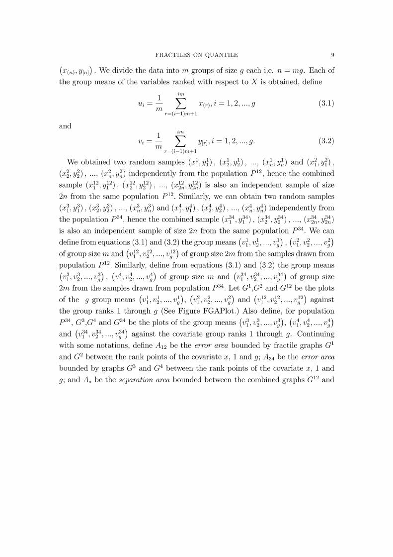
2m from the samples drawn from population P 34: Let G1,G2 and G12 be the plots
of the g group means�v11; v
12; :::; v
1g
�,�v21; v
22; :::; v
2g
�and
�v121 ; v
122 ; :::; v
12g
�against
the group ranks 1 through g (See Figure FGAPlot.) Also de�ne, for population
P 34; G3,G4 and G34 be the plots of the group means�v31; v
32; :::; v
3g
�,�v41; v
42; :::; v
4g
�and
�v341 ; v
342 ; :::; v
34g
�against the covariate group ranks 1 through g. Continuing
with some notations, de�ne A12 be the error area bounded by fractile graphs G1
and G2 between the rank points of the covariate x; 1 and g; A34 be the error area
bounded by graphs G3 and G4 between the rank points of the covariate x; 1 and
g; and A� be the separation area bounded between the combined graphs G12 and
FRACTILES ON QUANTILE 10
G34:
Figure 1: Fractile Graph
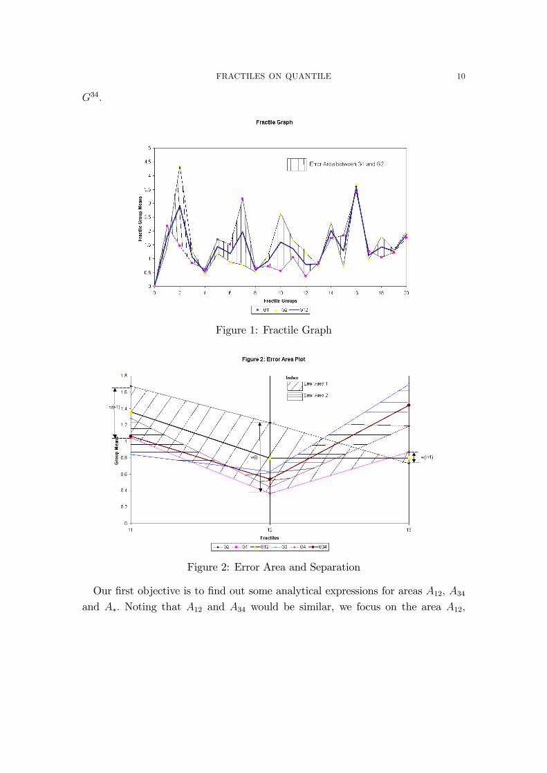
Figure 2: Error Area and Separation
Our �rst objective is to �nd out some analytical expressions for areas A12; A34and A�: Noting that A12 and A34 would be similar, we focus on the area A12;
FRACTILES ON QUANTILE 11
without loss of generality. Let us further de�ne the following quantities of di¤erence
of means in the two groups.
v1i � v2i = wi(12); i = 1; 2; :::; g
v3i � v4i = wi(34); i = 1; 2; :::; g
v12i � v34i = wi(�); i = 1; 2; :::; g
(3.3)
We can divide the area between G1 and G2 i.e. A12 into each constituent area
between the ordinates i and i + 1; say, A12(i): Let us summarize the construction
of the area as the following Proposition 1.
Proposition 1. (Takeuchi 1961) The error area bounded by graphs G1 and G2 isA12 =
Pg�1i=1 A12(i) where
A12(i) =1
2(jwij+ jwi+1j)� @ (wi; wi+1)
jwiwi+1jjwij+ jwi+1j
(3.4)
where @ (a; b) =
(0 if ab � 01 if ab < 0
Proof. Case 1: G1 and G2 does not cross between i and i + 1, that means thatwiwi+1 � 0:Area
�Ai(12)
�is essentially that of a trapezoid between parallel vertical lines at
i and i+ 1: Hence,
Ai(12) =1
2(jwij+ jwi+1j) if wiwi+1 � 0: (3.5)
Note that, we can de�ne w0 = 0; so A0(12) = 12(jw1j) : We can easily verify that
(3.4) holds here.
Case 2: G1 and G2 does cross between i and i+1, that means that wiwi+1 < 0:Area
�Ai(12)
�is essentially that of two equiangular triangles with their bases on
the vertical lines on i and i+1; or in other words the bases are unit distance apart.
Using the property of equiangular triangles, after construction, we can see that the
altitude (or rise) of the triangles would be proportional to the base (or run). Since
the bases of the triangles are jwij and jwi+1j respectively, if x is the altitude of thetriangle with base jwij we observe
jwijjwi+1j
=x
1� x) x =
jwijjwij+ jwi+1j
or 1� x =jwi+1j
jwij+ jwi+1j: (3.6)
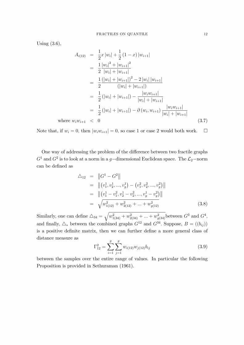
FRACTILES ON QUANTILE 12
Using (3.6),
Ai(12) =1
2x jwij+
1
2(1� x) jwi+1j
=1
2
jwij2 + jwi+1j2
jwij+ jwi+1j
=1
2
(jwij+ jwi+1j)2 � 2 jwij jwi+1j(jwij+ jwi+1j)
=1
2(jwij+ jwi+1j)�
jwiwi+1jjwij+ jwi+1j
=1
2(jwij+ jwi+1j)� @ (wi; wi+1)
jwiwi+1jjwij+ jwi+1j
where wiwi+1 < 0 (3.7)
Note that, if wi = 0; then jwiwi+1j = 0; so case 1 or case 2 would both work. �
One way of addressing the problem of the di¤erence between two fractile graphs
G1 and G2 is to look at a norm in a g�dimensional Euclidean space. The L2�normcan be de�ned as
412 = G1 �G2
=
�v11; v12; :::; v1g�� �v21; v22; :::; v2g� =
�v11 � v21; v12 � v22; :::; v
1g � v2g
� =
qw21(12) + w22(12) + :::+ w2g(12) (3.8)
Similarly, one can de�ne 434 =qw21(34) + w22(34) + :::+ w2g(34)between G
3 and G4;
and �nally, 4� between the combined graphs G12 and G34: Suppose, B = ((bij))
is a positive de�nite matrix, then we can further de�ne a more general class of
distance measure as
�212 =
gXi=1
gXj=1
wi(12)wj(12)bij (3.9)
between the samples over the entire range of values. In particular the following
Proposition is provided in Sethuraman (1961).
FRACTILES ON QUANTILE 13
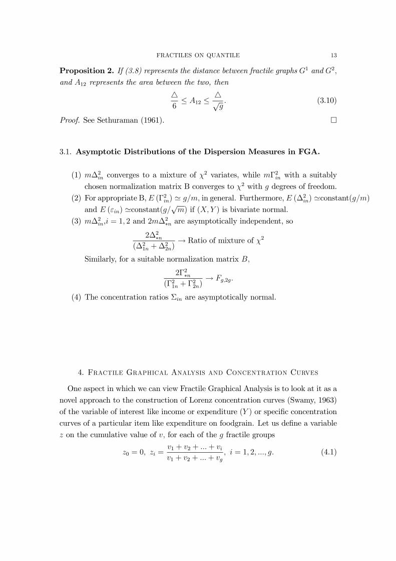
Proposition 2. If (3.8) represents the distance between fractile graphs G1 and G2;and A12 represents the area between the two, then
46� A12 �
4pg: (3.10)
Proof. See Sethuraman (1961). �
3.1. Asymptotic Distributions of the Dispersion Measures in FGA.
(1) m�2in converges to a mixture of �
2 variates, while m�2in with a suitably
chosen normalization matrix B converges to �2 with g degrees of freedom.
(2) For appropriate B,E (�2in) ' g=m; in general. Furthermore, E (�2in) 'constant(g=m)
and E ("in) 'constant(g=pm) if (X; Y ) is bivariate normal.
(3) m�2in,i = 1; 2 and 2m�
2�n are asymptotically independent, so
2�2�n
(�21n +�
22n)
! Ratio of mixture of �2
Similarly, for a suitable normalization matrix B;
2�2�n(�21n + �
22n)
! Fg;2g:
(4) The concentration ratios �in are asymptotically normal.
4. Fractile Graphical Analysis and Concentration Curves
One aspect in which we can view Fractile Graphical Analysis is to look at it as a
novel approach to the construction of Lorenz concentration curves (Swamy, 1963)
of the variable of interest like income or expenditure (Y ) or speci�c concentration
curves of a particular item like expenditure on foodgrain. Let us de�ne a variable
z on the cumulative value of v; for each of the g fractile groups
z0 = 0; zi =v1 + v2 + :::+ viv1 + v2 + :::+ vg
; i = 1; 2; :::; g: (4.1)
FRACTILES ON QUANTILE 14
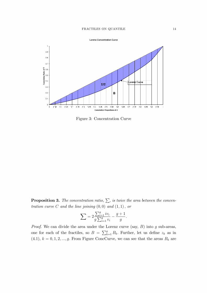
Figure 3: Concentration Curve
Proposition 3. The concentration ratio,P; is twice the area between the concen-
tration curve C and the line joining (0; 0) and (1; 1) ; orX= 2
Pgi=1 ivi
gPg
i=1 vi� g + 1
g:
Proof. We can divide the area under the Lorenz curve (say, B) into g sub-areas,
one for each of the fractiles, so B =Pg
k=1Bk: Further, let us de�ne zk as in
(4.1), k = 0; 1; 2; :::; g: From Figure ConcCurve, we can see that the areas Bk are

FRACTILES ON QUANTILE 15
trapezoids between the vertical lines at k� 1 and k on the x-axis, hence as zg = 1;gXk=1
Bk =
gXk=1
1
2(zk�1 + zk)
1
g
=1
2g[2 (z1 + z2 + :::+ zg�1) + zg]
=1
g
g�1Xk=1
zk +1
2g
=1
gPg
i=1 vi
g�1Xi=1
g�1Xk=i
vi +1
2g
=1
gPg
i=1 vi
gXi=1
(g � i) vi +1
2g
=1
gPg
i=1 vi
gXi=1
gvi �gXi=1
ivi
!+1
2g
= 1� 1
gPg
i=1 vi
gXi=1
ivi +1
2g
= 1 +1
2g�Pg
i=1 ivigPg
i=1 vi(4.2)
This means that the concentration ratioX= 2
"1
2�
gXk=1
Bk
#
= 1� 2�1 +
1
2g�Pg
i=1 ivigPg
i=1 vi
�=
2Pg
i=1 ivigPg
i=1 vi� g + 1
g: (4.3)
�
Lorenz curves or more generally speci�c concentration curves are the most obvi-
ous generalizations of fractile graphical analysis method to measures of inequality
or dispersion. This tool has been extensively used by authors like N. S. Iyengar
to estimate Engel curves and Engel elasticities from survey data (Iyengar, 1960,
1964). We would also see later in how the area under the speci�c concentration

FRACTILES ON QUANTILE 16
curve weakly converges to the function of a standard Brownian motion process
and a convolution of a independent Brownian Bridge process.
5. Fractile Regression
Our objective in this proposal is to look at the age-old problem of the e¤ect of the
covariates on distributions. Linear regression has always been the cornerstone of
such an analysis where we investigate at the e¤ects of the x-variables or covariates
on the response variable y. A very simple example of that could be the e¤ect
of educational quali�cation measured in years of education on income or future
income. It could be argued that educational quali�cation is a proxy for ability,
hence higher educational quali�cation would lead to higher earning. However,
performing simple linear regression on this somewhat naive model of "Returns to
Education" misses some major parts of the story. First, the story of endogeneity,
that is to say that it is very rare that education is randomly assigned, so individuals
choose education based on their ability and opportunity cost. Hence it would be
wrong to assign the credit of higher income solely to education, there could quite a
few omitted variables. In fact, the error term " in the population linear regression
model, i.e.
y = �0 + �1x+ "
where y is, say, log of income and x is the number of years of education, �0 and �1are the partial regression coe¢ cients, might be correlated with the independent
variable x - problem often times referred to as "endogeneity" in Econometrics.
However, the problem we are trying to address is not directly related to endo-
geneity, but the other aspect of the story missed by simple linear regression. It
is very likely that people with high ability or high educational quali�cation might
command a much higher salary for one extra year of education compared with
someone with low ability or education. Linear regression fails to capture this "dif-
ferential" treatment of the covariates or in particular "fractiles of the covariates."
So instead of looking at regression of y on x we should be looking at the regression
of Y grouped according to fractiles of X, i.e., we can answer the question for the
bottom 10% of educational quali�cation in the society what is the e¤ect of one
more year of education all else remaining the same. This really brings us to the
classical problem of non-parametric regression analysis. Let me brie�y describe
three very close neighbors in the �eld of regression analysis.
FRACTILES ON QUANTILE 17
In non-parametric (Kernel-based) regression analysis we consider Yi � N (m (xi) ; �2) ;
i = 1; 2; :::; n; where conditional mean function m (:) satis�es some regularity or
smoothness conditions. Broadly, we can de�ne the Nadaraya-Watson type location
or regression estimator with the smoothing kernel K (:) and bandwidth h as
mNW (xo) = arg min�o2R
nXi=1
(yi � �o)2K
�x� xih
�=
nXi=1
WNWin (x) yi (5.1)
We can think of replacing xi by a monotonic rank-score of xi and use the
weighted least squares type method as well. "Bandwidth" can be de�ned either in
terms of actual width (kernel type) or the number of observations (nearest neighbor
type). In Nearest Neighbor type regression estimate we replace x by the empirical
distribution function Fn (x) in Equation (5.1) to get
mNN (xo) = arg min�o2R
nXi=1
(yi � �o)2K
�Fn (x)� Fn (xi)
hn
�=
nXi=1
WNNin (x) yi:
(5.2)
The major advantage that k-Nearest Neighbor type estimator has over the tra-
ditional kernel based estimator is that the former only depends on the ranks of
X1; X2; :::; Xn: Hence, if F (x) is continuous the problem gets transformed to much
more tractable problem of estimating a regression function at F (x0) with the X-
sample being uniformly distributed over [0; 1] : Its convergence properties in mean
square has also been studied by Yang (1981). Stute (1984) showed that k-Nearest
Neighbor type estimates are asymptotically normal if E [Y 2] <1; is much weaker
than the conditions needed for existence of the Nadaraya-Watson type regression
estimates like existence of the PDF f (:) of X and that E jY j3 < 1 (Schuster
1972).
In quantile regression, we look at the regression counterpart of univariate � th
quantile of the dependent variable y is de�ned as
� (�) = argmina2R
nXi=1
�� (yi � a) , (5.3)
where �t (u) = (� � I (u < 0))u is often referred to as the check function.
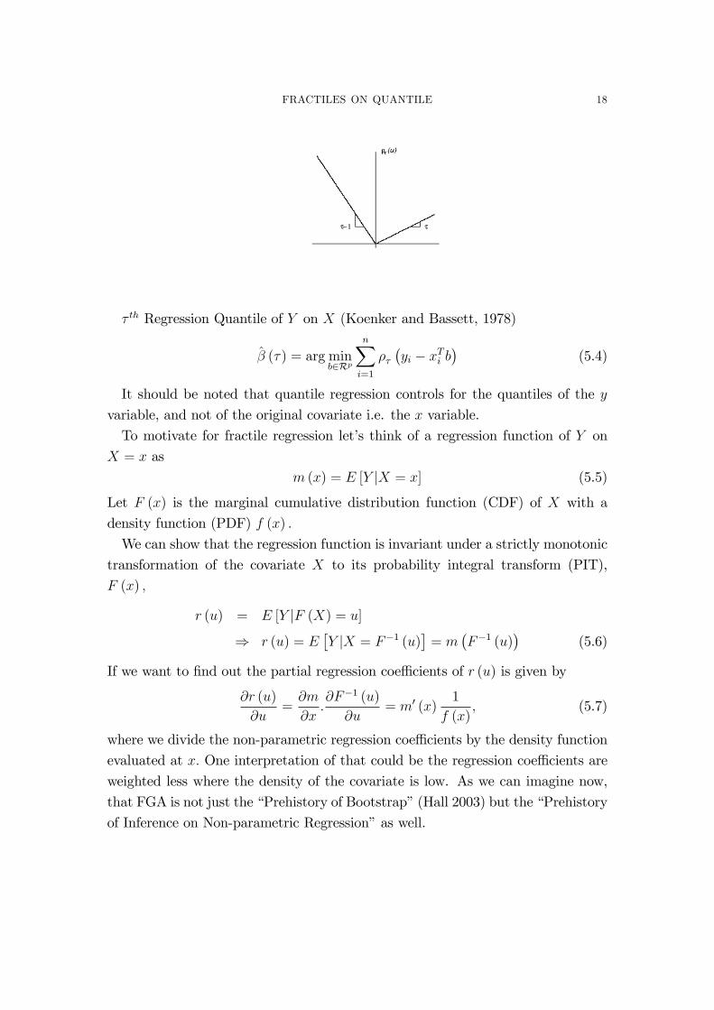
FRACTILES ON QUANTILE 18
� th Regression Quantile of Y on X (Koenker and Bassett, 1978)
� (�) = arg minb2Rp
nXi=1
���yi � xTi b
�(5.4)
It should be noted that quantile regression controls for the quantiles of the y
variable, and not of the original covariate i.e. the x variable.
To motivate for fractile regression let�s think of a regression function of Y on
X = x as
m (x) = E [Y jX = x] (5.5)
Let F (x) is the marginal cumulative distribution function (CDF) of X with a
density function (PDF) f (x) :
We can show that the regression function is invariant under a strictly monotonic
transformation of the covariate X to its probability integral transform (PIT),
F (x) ;
r (u) = E [Y jF (X) = u]
) r (u) = E�Y jX = F�1 (u)
�= m
�F�1 (u)
�(5.6)
If we want to �nd out the partial regression coe¢ cients of r (u) is given by
@r (u)
@u=@m
@x:@F�1 (u)
@u= m0 (x)
1
f (x); (5.7)
where we divide the non-parametric regression coe¢ cients by the density function
evaluated at x: One interpretation of that could be the regression coe¢ cients are
weighted less where the density of the covariate is low. As we can imagine now,
that FGA is not just the �Prehistory of Bootstrap�(Hall 2003) but the �Prehistory
of Inference on Non-parametric Regression�as well.
FRACTILES ON QUANTILE 19
6. Properties of Fractile Regression Function and their ranks
Suppose X has a distribution function F(x) ; the conditional distribution of Y
given X = x is G (yjX = x) = Gx:
Lemma 1. (Bhattacharya �74) If X has a continuous distribution function F (:) ;the induced order statistics Y[1]; Y[2]; :::; Y[n] are conditionally independent given
X1; X2; :::; Xnwith conditional CDFs Gx(1) ; Gx(2) ; :::; Gx(n) :
Proof. De�ne X = (X1; X2; :::; Xn)0 ; be a multivariate random variable and x =
(x1; x2; :::; xn)0 2 Rn: Now consider a mapping � (k;X) = j if X(k) = Xj )
� (k;X) = j if Y[j] = Yj (we can call � (k;X) an order statistic index �nder func-
tion.) Immediately, we can see that for X almost everywhere � (k;X) is uniquely
de�ned for all k 2 f1; 2; 3; :::; ng :
P�Y[1] � yj1 ; Y[2] � yj2 ; :::; Y[n] � yjnjX = x
�= P
�Y�(1;X) � yj1 ; Y�(2;X) � yj2 ; :::; Y�(n;X) � yjnjX = x
�= P
�Yj1 � yj1 ; Yj2 � yj2 ; :::; Yj2 � yjnjX =(x1; x2; :::; xn)
0�= P (Yj1 � yj1jXj1 = xj1 ; Yj2 � yj2jXj2 = xj2 ; :::; Yj2 � yjnjXjn = xjn)
= P (Yj1 � yj1jXj1 = xj1)P (Yj2 � yj2jXj2 = xj2) :::P (Yj2 � yjnjXjn = xjn)
= Gxj1 (yj1)Gxj2 (yj2) :::Gxjn (yjn)
since (Xi; Yi)0 ; i = 1; 2::::; n are independent and identically distributed random
variables that have a continuos distribution function. In general, for k = 1; 2; :::; n;this
argument will go through for any permutation � (k;X) of f1; 2; :::; ng : �
Theorem 1. Let X have a continuous distribution F (x) ; and the distribution
of Y given X = x is also continuous and denoted by Gx (y) : Then given any
1 � r1 < r2 < ::: < rk � n for any �xed k � n;
P�Y[ri] � yi; 1 � i � k
�= E
"kYi=1
Gx(ri)�yijX(ri) = x(ri)
�#: (6.1)
Proof. Applying lemma 1 we can immediately see that conditional on X = x
i.e.,(X1; X2; :::; Xn)0 = (x1; x2; :::; xn)
0 ;
P�Y[ri] � yi; 1 � i � kjX = x
�=
kYi=1
Gx(ri)�yijX(ri) = x(ri)
�: (6.2)
FRACTILES ON QUANTILE 20
The result of the theorem follows from an application of the law of iterated expec-
tation. �
Theorem 2. (David, O�Connell and Yang �77) Under the above regularity con-ditions, where in �1 = P (X < x; Y < y); �2 = P (X < x; Y > y); �3 = P (X >
x; Y < y) and �4 = P (X > x; Y > y), de�ning R (:) as the rank function,
P�R�Y[r]�= s�
= n
Z 1
�1
Z 1
�1
min(r�1;s�1)Xk=0
(n� 1)!k! (r � 1� k)! (s� 1� k)! (n� r � s+ 1 + k)!
��k1�r�1�k2 �s�1�k3 �n�r�s+1+k4 dG (yjx) dF (x) : (6.3)
Proof. Our objective is to �nd out the probability distribution (or probability
mass function) of the rank of the rth induced order statistic (or rth concomi-
tant variable to the order statistics of X) when we have an iid sample (Xi; Yi)
i = 1; 2; :::; n from a continuous bivariate distribution function F (x; y) i.e. to
�nd P (Rank (Yj) = sjRank (Xj) = r) = P�R�Y[r]�= s�: We can illustrate the
problem using the following table
X(r) < x X(r) > x Row Total
Y(s) < y k s� 1� k s� 1Y(s) > y r � 1� k n� r � s+ 1 + k n� s
Col: Total r � 1 n� r n� 1
where k 2 f0; 1; 2; :::;min (r � 1; s� 1)g :Hence, if t=min (r � 1; s� 1) given X = x and Y = y;
P�R(Y[r]) = s
�=
tXk=0
(n� 1)!k! (s� 1� k)! (r � 1� k)! (n� r � s+ 1 + k)!
�
�k1�r�1�k2 �s�1�k3 �n�r�s+1+k4 :
FRACTILES ON QUANTILE 21
Since there are n such variables Y; the unconditional probability for any value of
X = x and Y = y
P�R(Y[r]) = s
�= n
Z 1
�1
Z 1
�1
tXk=0
(n� 1)!k! (s� 1� k)! (r � 1� k)! (n� r � s+ 1 + k)!
�
�k1�r�1�k2 �s�1�k3 �n�r�s+1+k4 dGx (y) dF (x) :
�
Theorem 3. (Yang �77) Suppose the marginal distribution of X has a density
function f (x) that is bounded away from 0 in a neighborhood of F�1 (�i) ; i =
1; 2; :::; k: Also assume that the conditional probability distribution of Y jX = x; Gx
at y1; y2; :::; yn are continuous at x:Then for 1 � r1 < r2 < ::: < rk � n such thatrin! �i 2 (0; 1) as n!1;
limn!1
P�Y[ri] � yi; 1 � i � k
�=
kYi=1
G�yijF�1 (�i)
�: (6.4)
Proof. This is an extension of the Theorem 1 in case the sample size diverges to
1: Suppose for some �xed k = 0; 1; 2; :::; n rin! �i 2 (0; 1) as n ! 1; then
for an absolutely continuous distribution function F (:) ; F�1�rin
�! F�1 (�i) as
n ! 1: This follows from the convergence of continuous functions of quantiles
of the Empirical Distribution Function (EDF) to the quantiles of the Cumulative
Distribution Function (CDF) (see for example Rao(1973) page 423 6f.2(i) :)
So as n!1 and �xed k; using Theorem 1, and thatGx (:) is a bounded continuous
(conditional distribution) function
limn!!1
P�Y[ri] � yi; 1 � i � k
�= lim
n!1
kYi=1
G�yijF�1
�rin
��=
kYi=1
G�yijF�1 (�i)
�:
�
Theorem 4. Suppose now that the joint distribution of (X; Y ) say p (x; y) is con-tinuous and is bounded by some function q (y) for all x in a neighborhood of
�� = F�1 (�) :Further suppose, the marginal density function f (x) of X exists
and is bounded away from 0 in a neighborhood of ��; 0 < � < 1: If rn! � as
FRACTILES ON QUANTILE 22
n!1; and if we de�ne Z = G (Y ) and Z� = G (Y jF (X) = �) = GF�1(�) (Y ) as
the unconditional and the conditional probability integral transforms of Y; then
(i) limn!1
E
24 R �Y[r]�n
!k35 = Z 1
�1Gk (y) dG
�yjF�1 (�)
�=
Z 1
�1ZkdZ� (6.5)
(ii) limn!1
P�R�Y[r]�� na
�= P
�Z � ajF�1 (�)
�= P [Z� � a] for 0 � a � 1:
(6.6)
Proof. (i)This proof is based on results in David and Galambos (1974) and Yang
(1977). For I fAg = 1; if A occurs, I fAg = 0 otherwise; and de�ning � (k;X) = j
if Y[k] = Yj, let�s �rst consider an expression
�R�Y[r]��k
=
"nXj=1
I�Yj � Y[r]
#k=
Xj1 6=j2 6=::: 6=jk 6=�(r;X)
I�Yj1 � Y[r]
I�Yj2 � Y[r]
:::I�Yjk � Y[r]
+O
�nk�1
�
FRACTILES ON QUANTILE 23
which implies the kth central moment of the rank of the rth induced order statistic is
E
24 R �Y[r]�n
!k35=
1
nk
Xj1 6=j2 6=::: 6=jk 6=�(r;X)
P�Yj1 � Y[r]; Yj2 � Y[r]; :::; Yjk � Y[r]
�+O
�n�1�
=1
nk
nXl=1
Xj1 6=j2 6=::: 6=jk 6=l
P (Yj1 � Yl; Yj2 � Yl; :::; Yjk � Yl; rank (Xl) = r) +O�n�1�
=n (n� 1) ::: (n� k)
nkP (Y1 � Yn; Y2 � Yn; :::; Yk � Yn; rank (Xn) = r) +O
�n�1�
=n (n� 1) ::: (n� k)
nk
kXl=0
�k
l
�
�P
0B@ Xi � Xn; Yi � Yn; i = 1; 2; :::; l;
Xi > Xn; Yi � Yn; i = l + 1; ::; k;
Exactly (r � 1� l) Xi � Xn; i = k + 1; ::; n
1CA+O�n�1�
=n (n� 1) ::: (n� k)
nk
kXl=0
�k
l
�Z 1
�1
�Z 1
�1p (x; y)l (G (y)� p (x; y))k�l f (yjx) dy
��
fr�l:n�kdx+O�n�1�
where f (yjx) is the density function of y given X = x; fr�l;n�k (:) is the density
function of X(r�l) out of a possible (n� k) X 0s: As n; r diverges to1; s.t. rn! �;
for �xed k; X(r�l) converges in probability to to �: Hence, we get using binomial
FRACTILES ON QUANTILE 24
expansion
limn!1
E
24 R �Y[r]�n
!k35 =
kXl=0
�k
l
��Z 1
�1p (�; y)l (G (y)� p (�; y))k�l f (yj�) dy
�
=
Z 1
�1
(kXl=0
�k
l
�p (�; y)l (G (y)� p (�; y))k�l
)f (yj�) dy
=
Z 1
�1fp (�; y) +G (y)� p (�; y)gk f (yj�) dy
=
Z 1
�1fG (y)gk dG (yjX = �)
=
Z 1
�1ZkdZ�
which proves result (i) :
(ii) Part (i) essentially implies that the kth moment of the normalized ranks of the
rth induced order statistics converges to the kth moment of a uniformly distributed
random variable conditional on the �th quantile. Hence, all the moments are
continuous and bounded. This implies that the distribution of the normalized
ranks are completely speci�ed by its moments, hence for some 0 � a � 1
P�R�Y[r]�� na
�= P
" R�Y[r]�
n
!� aj X(r) = x(r)
#
) limn!1
P�R�Y[r]�� na
�= lim
n!1P
" R�Y[r]�
n
!� aj X(r) = x(r)
#) lim
n!1P�R�Y[r]�� na
�= P
�G (y) � ajX = F�1 (�)
�= P [Z� � aj] :
�
This theorem simply implies that it is su¢ cient to work with the probability
integral transforms of the Y variable after conditioning for the rank of the X
variable.
Furthermore, the following corollary helps us to make inference on "fractile
groups."
FRACTILES ON QUANTILE 25
Corollary 1. Suppose now there are two sequences r and s such that as n!1;rn! �r and s
n! �s where 0 < �r < �s < 1; then for any 0 � a � 1 and all any i;
limn!1
P [R (Yi) � najr � R(Xi) � s]
=1
�s � �r
Z �s
�r
P�Z � ajF�1 (�)
�d�
=1
�s � �r
Z �s
�r
P (Z� � a) d�: (6.7)
Proof. For any n;
P [R (Yi) � na j r � R (Xi) � s]
=n
s� r + 1
sXj=r
P [R (Xi) = j]P [R (Yi) � na j R (Xi) = j]
=n
s� r + 1
sXj=r
1
nP�R�Y[j]�� na
�:
We also note that as n ! 1; rn! �r and s
n! �s where 0 < �r < �s < 1; using
Theorem 4
limn!1
sXj=r
1
nP�R�Y[j]�� na
�= lim
n!1
sXj=r
1
nP
�Z � a j F�1
�j
n
��
=
Z �s
�r
P�Z � a j F�1 (�)
�d�
=
Z �s
�r
P [Z� � a ] d�
using the Reimann Sum representation of an integral. �
6.1. Asymptotics of Fractile Regression Analysis. Let R (t) =R t0r (s) ds;
be the Cumulative Fractile Regression function, (Rao and Zhao, 1995) the
Rn (t) =1
n
[nt]Xj=1
y[j]; : (6.8)
is an estimate ofR (t) ; where [nt] is the largest integer less than or equal to nt. This
term can be interpreted as a normalized partial (Reimann) sum that converges the
area under the concentration curve (See Figure 3) upto point t; and is a measure

FRACTILES ON QUANTILE 26
of the total variability or dispersion in the induced order statistic Y among the
lowest 100t% of the population with respect to X:
Let the conditional variance of Y given X = x; be �2 (x) = V ar (Y jX = x) :We
can further de�ne the integrated volatility
(t) =
Z F�1(t)
�1�2 (x) dF (x) (6.9)
with the sample counterpart as
n (t) =
Z F�1n (t)
�1�2 (x) dFn (x) if
1
n� t � 1
= 0 otherwise. (6.10)
where Fn (x) is the EDF of X1; X2; :::; Xn:
Lemma 2. If �2 (x) is of bounded variation,
sup0�t�1
j n (t)� (t)j a:s:! 0: (6.11)
Proof. Using a change of variable of U = F (X) ; and applying integration by parts
on expression for integrated volatility,
(t) =
Z F�1(t)
�1�2 (x) dF (x)
=
Z t
0
�2�F�1 (u)
�du
= �2�F�1 (t)
�t�Z t
0
ud�2: (6.12)
Now applying technique in equation (6.12) to equation (6.10),
n (t) =
Z F�1n (t)
�1�2 (x) dFn (x)
=
Z t
0
�2�F�1n (u)
�du
= �2�F�1n (t)
�t�Z t
0
ud�2: (6.13)
From equations (6.12) and (6.13),
n (t)� (t) =��2�F�1n (t)
�� �2
�F�1 (t)
��t: (6.14)
FRACTILES ON QUANTILE 27
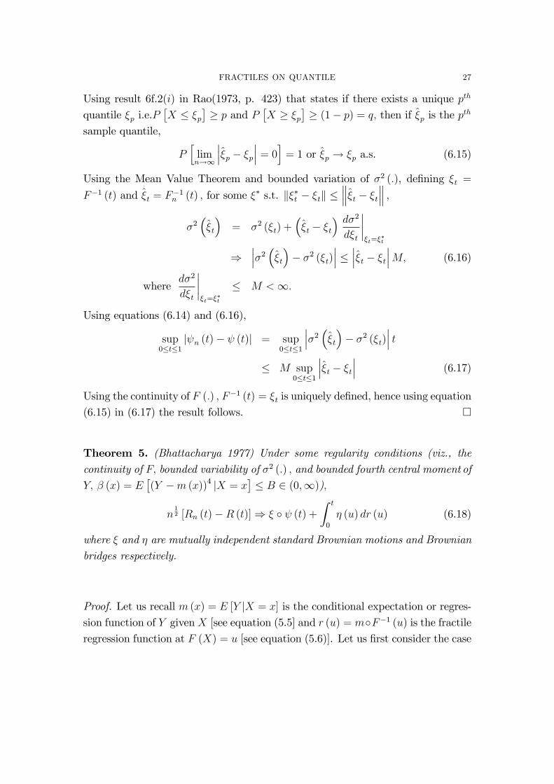
Using result 6f.2(i) in Rao(1973, p. 423) that states if there exists a unique pth
quantile �p i.e.P�X � �p
�� p and P
�X � �p
�� (1� p) = q; then if �p is the p
th
sample quantile,
Phlimn!1
����p � �p
��� = 0i = 1 or �p ! �p a.s. (6.15)
Using the Mean Value Theorem and bounded variation of �2 (:), de�ning �t =
F�1 (t) and �t = F�1n (t) ; for some �� s.t. k��t � �tk � �t � �t
;�2��t
�= �2 (�t) +
��t � �t
� d�2d�t
�����t=�
�t
)����2 ��t�� �2 (�t)
��� � ����t � �t
���M; (6.16)
whered�2
d�t
�����t=�
�t
� M <1:
Using equations (6.14) and (6.16),
sup0�t�1
j n (t)� (t)j = sup0�t�1
����2 ��t�� �2 (�t)��� t
� M sup0�t�1
����t � �t
��� (6.17)
Using the continuity of F (:) ; F�1 (t) = �t is uniquely de�ned, hence using equation
(6.15) in (6.17) the result follows. �
Theorem 5. (Bhattacharya 1977) Under some regularity conditions (viz., thecontinuity of F; bounded variability of �2 (:) ; and bounded fourth central moment of
Y; � (x) = E�(Y �m (x))4 jX = x
�� B 2 (0;1));
n12 [Rn (t)�R (t)]) � � (t) +
Z t
0
� (u) dr (u) (6.18)
where � and � are mutually independent standard Brownian motions and Brownian
bridges respectively.
Proof. Let us recall m (x) = E [Y jX = x] is the conditional expectation or regres-
sion function of Y given X [see equation (5.5] and r (u) = m�F�1 (u) is the fractileregression function at F (X) = u [see equation (5.6)]. Let us �rst consider the case
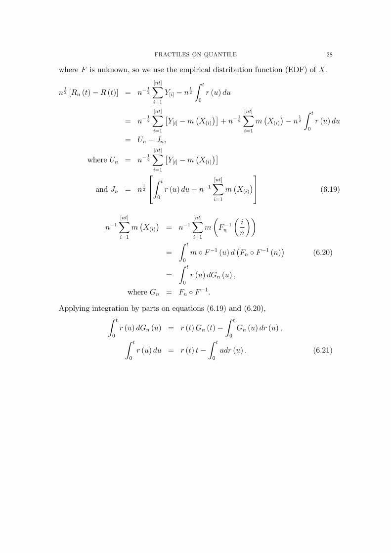
FRACTILES ON QUANTILE 28
where F is unknown, so we use the empirical distribution function (EDF) of X:
n12 [Rn (t)�R (t)] = n�
12
[nt]Xi=1
Y[i] � n12
Z t
0
r (u) du
= n�12
[nt]Xi=1
�Y[i] �m
�X(i)
��+ n�
12
[nt]Xi=1
m�X(i)
�� n
12
Z t
0
r (u) du
= Un � Jn;
where Un = n�12
[nt]Xi=1
�Y[i] �m
�X(i)
��and Jn = n
12
24Z t
0
r (u) du� n�1[nt]Xi=1
m�X(i)
�35 (6.19)
n�1[nt]Xi=1
m�X(i)
�= n�1
[nt]Xi=1
m
�F�1n
�i
n
��=
Z t
0
m � F�1 (u) d�Fn � F�1 (n)
�(6.20)
=
Z t
0
r (u) dGn (u) ;
where Gn = Fn � F�1:
Applying integration by parts on equations (6.19) and (6.20),Z t
0
r (u) dGn (u) = r (t)Gn (t)�Z t
0
Gn (u) dr (u) ;Z t
0
r (u) du = r (t) t�Z t
0
udr (u) : (6.21)
FRACTILES ON QUANTILE 29
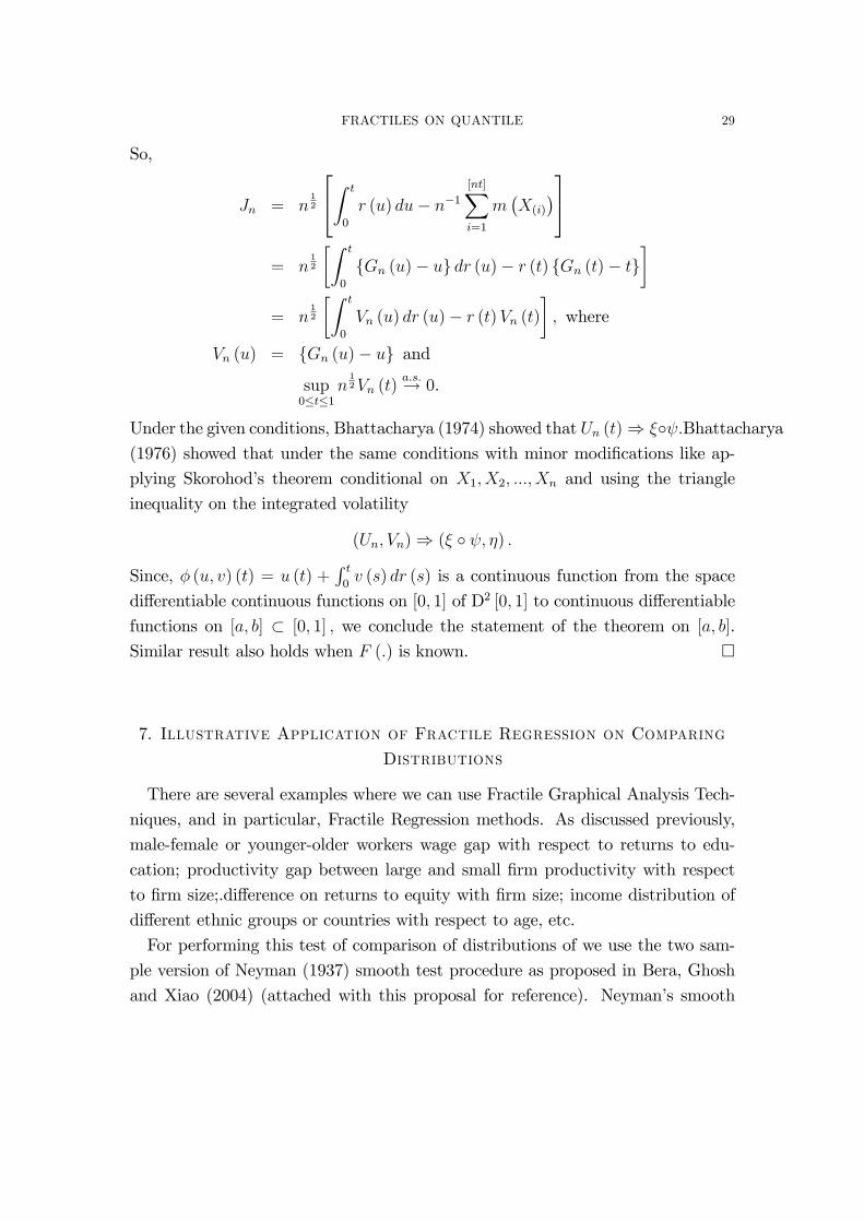
So,
Jn = n12
24Z t
0
r (u) du� n�1[nt]Xi=1
m�X(i)
�35= n
12
�Z t
0
fGn (u)� ug dr (u)� r (t) fGn (t)� tg�
= n12
�Z t
0
Vn (u) dr (u)� r (t)Vn (t)
�; where
Vn (u) = fGn (u)� ug and
sup0�t�1
n12Vn (t)
a:s:! 0.
Under the given conditions, Bhattacharya (1974) showed that Un (t)) �� :Bhattacharya(1976) showed that under the same conditions with minor modi�cations like ap-
plying Skorohod�s theorem conditional on X1; X2; :::; Xn and using the triangle
inequality on the integrated volatility
(Un; Vn)) (� � ; �) :
Since, � (u; v) (t) = u (t) +R t0v (s) dr (s) is a continuous function from the space
di¤erentiable continuous functions on [0; 1] of D2 [0; 1] to continuous di¤erentiable
functions on [a; b] � [0; 1] ; we conclude the statement of the theorem on [a; b].
Similar result also holds when F (:) is known. �
7. Illustrative Application of Fractile Regression on Comparing
Distributions
There are several examples where we can use Fractile Graphical Analysis Tech-
niques, and in particular, Fractile Regression methods. As discussed previously,
male-female or younger-older workers wage gap with respect to returns to edu-
cation; productivity gap between large and small �rm productivity with respect
to �rm size;.di¤erence on returns to equity with �rm size; income distribution of
di¤erent ethnic groups or countries with respect to age, etc.
For performing this test of comparison of distributions of we use the two sam-
ple version of Neyman (1937) smooth test procedure as proposed in Bera, Ghosh
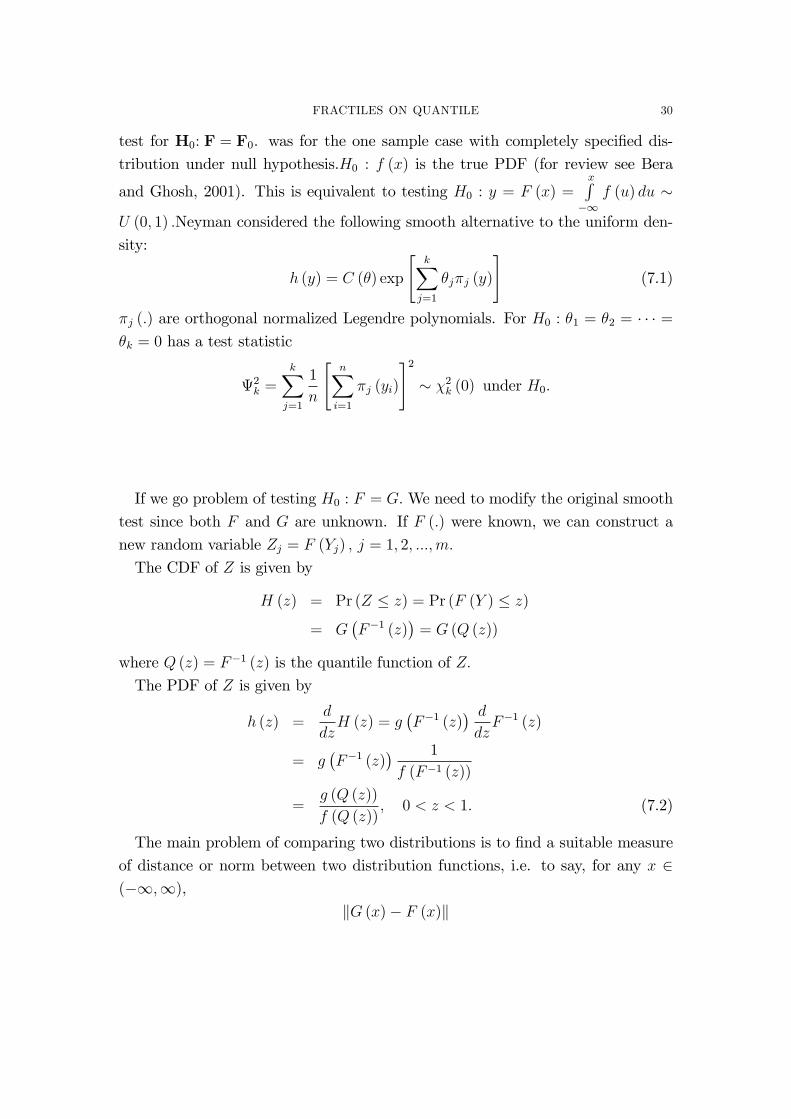
and Xiao (2004) (attached with this proposal for reference). Neyman�s smooth
FRACTILES ON QUANTILE 30
test for H0: F = F0. was for the one sample case with completely speci�ed dis-
tribution under null hypothesis.H0 : f (x) is the true PDF (for review see Bera
and Ghosh, 2001). This is equivalent to testing H0 : y = F (x) =xR
�1f (u) du �
U (0; 1) :Neyman considered the following smooth alternative to the uniform den-
sity:
h (y) = C (�) exp
"kXj=1
�j�j (y)
#(7.1)
�j (:) are orthogonal normalized Legendre polynomials. For H0 : �1 = �2 = � � � =�k = 0 has a test statistic
2k =
kXj=1
1
n
"nXi=1
�j (yi)
#2� �2k (0) under H0:
If we go problem of testing H0 : F = G:We need to modify the original smooth
test since both F and G are unknown. If F (:) were known, we can construct a
new random variable Zj = F (Yj) ; j = 1; 2; :::;m:
The CDF of Z is given by
H (z) = Pr (Z � z) = Pr (F (Y ) � z)
= G�F�1 (z)
�= G (Q (z))
where Q (z) = F�1 (z) is the quantile function of Z:
The PDF of Z is given by
h (z) =d
dzH (z) = g
�F�1 (z)
� ddzF�1 (z)
= g�F�1 (z)
� 1
f (F�1 (z))
=g (Q (z))
f (Q (z)); 0 < z < 1: (7.2)
The main problem of comparing two distributions is to �nd a suitable measure
of distance or norm between two distribution functions, i.e. to say, for any x 2(�1;1),
kG (x)� F (x)k
FRACTILES ON QUANTILE 31
If a density function exists over the support of F and G; then for any t 2 (0; 1)this problem to be equivalent to the distance��G � F�1 (t)� t
�� :Under H0 : G = F; G � F�1 (t) = t: In fact, the h (z) in (7.2) is the corresponding
PDF for the distribution function G � F�1 de�ned over (0; 1) : The PDF h (z) is aratio of two densities; and itself is a valid density function. Therefore, we will call
it the Ratio Density Function (RDF) (Bera, Ghosh and Xiao, 2004).
When H0 : F = G is true (i.e. f = g) then from (7.2), h (z) = g(Q(x))f(Q(x))
= 1; 0 <
z < 1. Z has the Uniform density in (0; 1) :That means irrespective of what F
and G are, the two-sample testing problems can be converted into testing only one
kind of hypothesis; namely, uniformity of a transformed random variable.
For the two sample case with unknown F and G the Smooth test statistic is
2k =kXl=1
u2l ; ul =1pm
mXj=1
�l (zj) ; l = 1; 2; :::; k
zj = F (yj) =
Z yj
�1f (!) d!; j = 1; 2; :::;m.
Under H0 : F = G;2kD! �2k:
The test has k components. Each component provides information regarding
speci�c departures from H0 : F = G:
However, in practice F (:) is unknown. We use the Empirical Distribution Func-
tion,
Fn (x) =1
n
nXi=1
I (Xi � x) ; zj = Fn (yj)
2k =
kXl=1
1
m
"mXj=1
�l (zj)
#2The following two theorems [for proof and details see Bera, Ghosh and Xiao (2004)]
provide some restrictions on relative sample sizes for consistent asymptotic �2
distribution of the test statistic, and also to minimize size distortion of the two
sample smooth test of comparing two distributions.
Theorem 6. If m log lognn
! 0 as m;n!1 then 2k �2k = op (1) :

FRACTILES ON QUANTILE 32
Theorem 7. The optimal relative magnitude of m and n for minimum size dis-
tortion is given by m = O (pn) :
For �nite sample, for each �xed n2, we may divide the index set N = f1; : : : ; nginto two mutually exclusive and exhaustive (large) sets N1 and N2 with cardinal-
ities n1 and n2; where n1 + n2 = n; and de�ne the training set
Z1 = f(Xj); j 2 N1gand the testing set
Z2 = f(Xj); j 2 N2g:Then we can estimate F (�) using data Z1 and construct
Fn1 (Xi) =1
n1
Xj2N1
I (Xj � Xi) , for i 2 N2:
Z1 and Z2 are from the same distribution F , F (Xi) (i 2 N2) are uniformly
distributed and Fn1 (Xi) provides an estimator for the uniform distribution, we
may compare it with the CDF of standard uniform, say, using some criterion
function1
n2
Xi2N2
d(Fn1 (Xi) ; U [0; 1])
and take average over R replications
1
R
RXr=1
"1
n2
Xi2N2
d(F rn1 (Xi) ; U [0; 1])
#For each value of n2, we can calculate the above criterion function. We may
choose n2 that minimizes the above criterion.
Finally, we choose
m =n2n1� n:
The above method may have applications in more general settings. This is a
cross-validation type procedure to select sample size.
One of the main problems we would investigate is the distributions of mutual
fund in�ows with before and after taxes with returns as covariate.(Poterba and
Bergstressor, 2002). Means of mutual fund in�ow distributions are di¤erent before
and after taxes with past year returns as covariate.(Poterba and Bergstressor,
2002). "Return chasing" behavior among investors and excessive risk taking among
FRACTILES ON QUANTILE 33
fund managers (Chevalier and Ellison, 1997). Higher cash �ow volatility and Fund
performance might have a negative relationship (Edelen, 1999, Rakowski, 2002).
In�ow distribution convey sentiments about stocks (Frazenni and Lamont, 2005).
We want investigate how these distributions are di¤erent when we control for the
fractiles of returns, hence we can predict the mutual fund in�ow based on pre-tax
or post-tax return information. This paper documented that mutual funds with
heavily taxed returns have lower subsequent in�ows compared to ones with lower
tax burdens. Our objective is to see if there is evidence in the in�ow distributions to
show whether higher moments including volatility or skewness and kurtosis terms
of in�ow distributions are a¤ected by tax exposure. Bergstresser and Poterba
(2002) considered US domestic equity mutual funds data on January Releases
from Morningstar Principia database with some conditions from 1993-1999.
For our current exposition we will only focus on the 1999 equity mutual fund
returns and in�ow data with similar characteristics. Bergstresser and Poterba
(2002) found that after-tax returns do indeed have more in�uence on cash in�ows
on mutual funds, however they did not test whether higher order moments of the
in�ow distribution are a¤ected by after tax returns.
FRACTILES ON QUANTILE 34
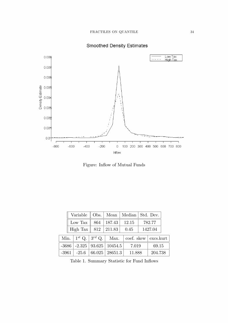
Figure: In�ow of Mutual Funds
Variable Obs. Mean Median Std. Dev.
Low Tax 864 187.43 12.15 782.77
High Tax 812 211.83 0.45 1427.04
Min. 1st Q. 3rd Q. Max. coef. skew excs.kurt
-3686 -2.325 93.625 10454.5 7.019 69.15
-3961 -25.6 66.025 28651.3 11.888 204.738
Table 1. Summary Statistic for Fund In�ows
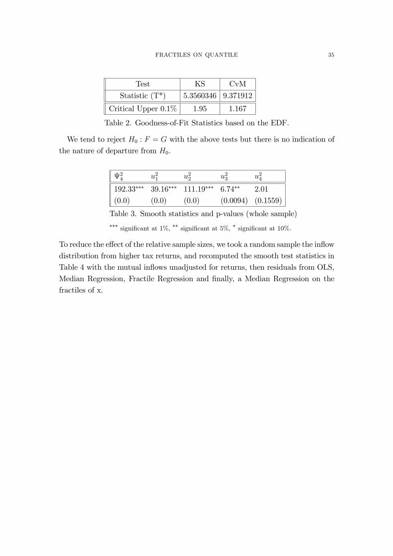
FRACTILES ON QUANTILE 35
Test KS CvM
Statistic (T*) 5.3560346 9.371912
Critical Upper 0.1% 1.95 1.167
Table 2. Goodness-of-Fit Statistics based on the EDF.
We tend to reject H0 : F = G with the above tests but there is no indication of
the nature of departure from H0:
24 u21 u22 u23 u24
192.33��� 39.16��� 111.19��� 6.74�� 2.01
(0.0) (0.0) (0.0) (0.0094) (0.1559)
Table 3. Smooth statistics and p-values (whole sample)��� signi�cant at 1%, �� signi�cant at 5%, � signi�cant at 10%.
To reduce the e¤ect of the relative sample sizes, we took a random sample the in�ow
distribution from higher tax returns, and recomputed the smooth test statistics in
Table 4 with the mutual in�ows unadjusted for returns, then residuals from OLS,
Median Regression, Fractile Regression and �nally, a Median Regression on the
fractiles of x.
FRACTILES ON QUANTILE 36
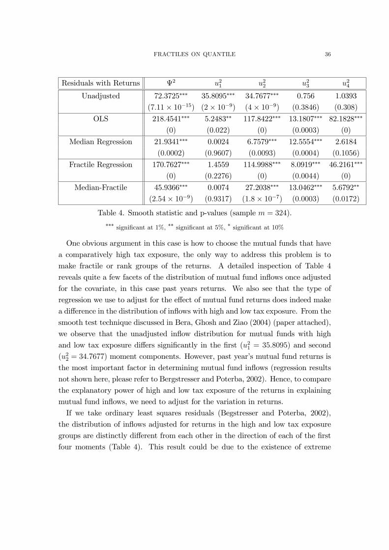
Residuals with Returns 2 u21 u22 u23 u24
Unadjusted 72.3725��� 35.8095��� 34.7677��� 0.756 1.0393
(7:11� 10�15) (2� 10�9) (4� 10�9) (0:3846) (0:308)
OLS 218.4541��� 5.2483�� 117.8422��� 13.1807��� 82.1828���
(0) (0:022) (0) (0:0003) (0)
Median Regression 21.9341��� 0.0024 6.7579��� 12.5554��� 2.6184
(0:0002) (0:9607) (0:0093) (0:0004) (0:1056)
Fractile Regression 170.7627��� 1.4559 114.9988��� 8.0919��� 46.2161���
(0) (0:2276) (0) (0:0044) (0)
Median-Fractile 45.9366��� 0.0074 27.2038��� 13.0462��� 5.6792��
(2:54� 10�9) (0:9317) (1:8� 10�7) (0:0003) (0:0172)
Table 4. Smooth statistic and p-values (sample m = 324).��� signi�cant at 1%, �� signi�cant at 5%, � signi�cant at 10%
One obvious argument in this case is how to choose the mutual funds that have
a comparatively high tax exposure, the only way to address this problem is to
make fractile or rank groups of the returns. A detailed inspection of Table 4
reveals quite a few facets of the distribution of mutual fund in�ows once adjusted
for the covariate, in this case past years returns. We also see that the type of
regression we use to adjust for the e¤ect of mutual fund returns does indeed make
a di¤erence in the distribution of in�ows with high and low tax exposure. From the
smooth test technique discussed in Bera, Ghosh and Ziao (2004) (paper attached),
we observe that the unadjusted in�ow distribution for mutual funds with high
and low tax exposure di¤ers signi�cantly in the �rst (u21 = 35:8095) and second
(u22 = 34:7677) moment components. However, past year�s mutual fund returns is
the most important factor in determining mutual fund in�ows (regression results
not shown here, please refer to Bergstresser and Poterba, 2002). Hence, to compare
the explanatory power of high and low tax exposure of the returns in explaining
mutual fund in�ows, we need to adjust for the variation in returns.
If we take ordinary least squares residuals (Begstresser and Poterba, 2002),
the distribution of in�ows adjusted for returns in the high and low tax exposure
groups are distinctly di¤erent from each other in the direction of each of the �rst
four moments (Table 4). This result could be due to the existence of extreme
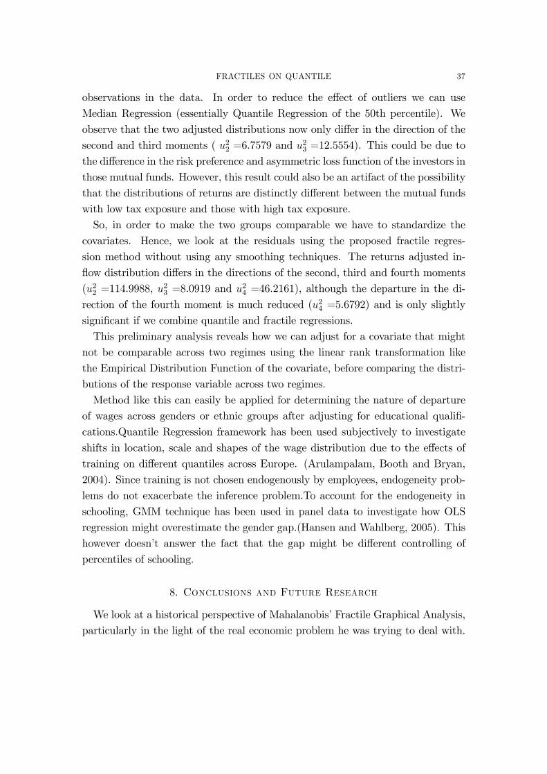
FRACTILES ON QUANTILE 37
observations in the data. In order to reduce the e¤ect of outliers we can use
Median Regression (essentially Quantile Regression of the 50th percentile). We
observe that the two adjusted distributions now only di¤er in the direction of the
second and third moments ( u22 =6.7579 and u23 =12.5554). This could be due to
the di¤erence in the risk preference and asymmetric loss function of the investors in
those mutual funds. However, this result could also be an artifact of the possibility
that the distributions of returns are distinctly di¤erent between the mutual funds
with low tax exposure and those with high tax exposure.
So, in order to make the two groups comparable we have to standardize the
covariates. Hence, we look at the residuals using the proposed fractile regres-
sion method without using any smoothing techniques. The returns adjusted in-
�ow distribution di¤ers in the directions of the second, third and fourth moments
(u22 =114.9988, u23 =8.0919 and u
24 =46.2161), although the departure in the di-
rection of the fourth moment is much reduced (u24 =5.6792) and is only slightly
signi�cant if we combine quantile and fractile regressions.
This preliminary analysis reveals how we can adjust for a covariate that might
not be comparable across two regimes using the linear rank transformation like
the Empirical Distribution Function of the covariate, before comparing the distri-
butions of the response variable across two regimes.
Method like this can easily be applied for determining the nature of departure
of wages across genders or ethnic groups after adjusting for educational quali�-
cations.Quantile Regression framework has been used subjectively to investigate
shifts in location, scale and shapes of the wage distribution due to the e¤ects of
training on di¤erent quantiles across Europe. (Arulampalam, Booth and Bryan,
2004). Since training is not chosen endogenously by employees, endogeneity prob-
lems do not exacerbate the inference problem.To account for the endogeneity in
schooling, GMM technique has been used in panel data to investigate how OLS
regression might overestimate the gender gap.(Hansen and Wahlberg, 2005). This
however doesn�t answer the fact that the gap might be di¤erent controlling of
percentiles of schooling.
8. Conclusions and Future Research
We look at a historical perspective of Mahalanobis�Fractile Graphical Analysis,
particularly in the light of the real economic problem he was trying to deal with.
FRACTILES ON QUANTILE 38
We reevaluate his contribution to the statistics and econometrics literature, as a
precursor to k-Nearest Neighbor regression techniques. One of our main objec-
tives in this paper is to de�ne a new form of non-parametric regression namely
Fractile Regression. We look at the di¤erent regression methods like kernel based
non-parametric regression, quantile regression and fractile regression through an
illustrative examples in in�ow distribution of mutual fundsWe look at some asymp-
totic properties of Fractile Regression. We look at some empirical examples like
the distribution of mutual fund in�ow with pre-tax and after tax returns (Poterba
and Bergstresser, 2002).
References
[1] Altman, N.S. "An Introduction to Kernel and Nearest-Neighbor Nonparametric Regression,"
The American Statistician, Volume 46:3,. pp. 175-185, 1992.
[2] Abdel-Ghany, M., Gehlken, A. and J. L. Silver. " Estimation of income elasticities from
Lorenz concentration curves: Application to Canadian micro-data," International Journal
of Consumer Studies, Volume 26:4, pp.278, 2002.
[3] Arulampalam, W., A. L. Booth and M. L. Bryan. "Are there Asymmetries in the E¤ects of
Training on Conditional Male Wage Distribution?" IZA Discussion Paper No. 984, Mimeo,
2004.
[4] Bera, A. K. and A. Ghosh. "Neyman�s Smooth Test and Its Applications in Econometrics,"
In Handbook of Applied Econometrics and Statistical Inference, Eds. A. Ullah, A. Wan and
A. Chaturvedi, Marcel Dekker: New York, pp. 177-249, 2001.
[5] Bera, A. K., A. Ghosh and Z. Xiao. "Smooth Test for Copmaring Equality of Two Distrib-
utions," Working Paper, Singapore Management University, 2004.
[6] Bergstresser, D. and J. Poterba. "Do after-tax returns a¤ect mutual fund in�ows?" Journal
of Financial Economics 63, pp.381-414, 2002.
[7] Bhattacharya, P. K. "On an analog of Regression Analysis," The Annals of Mathematical
Statistics, Vol. 34:4, pp. 1459-1473, 1963.
[8] Bhattacharya, P. K. "Convergence of sample paths of normalized sums of induced order
statistics," Annals of Statistics 2, pp. 1034-1039, 1974.
[9] Bhattacharya, P. K. "An invariance principle in regression analysis," Annals of Statistics 4,
pp. 621-624, 1976.
[10] Bhattacharya, P. K. "Induced Order Statistics: Theory and Applications," In Handbook of
Statistics, Vol. 4, P.R. Krishnaiah and P.K. Sen, Eds. Elsevier: New York, pp.383-403, 1984.
[11] Bhattacharya, P. K. and A. K. Gangopadhyay. "Kernel and Nearest-Neighbor Estimation
of a Conditional Quantile," The Annals of Statistics, Vol. 18:3, pp. 1400-1415, 1990.

FRACTILES ON QUANTILE 39
[12] Bhattacharya, P. K. and H.-G. Müller. "Asymptotics for Nonparametric Regression,"
Sankhya, Series A, Volume dedicated to the memory of P. C. Mahalanobis 55:3, pp. 420-441,
1993.
[13] Boos, D.D. "Minimum Distance estimators for Location and Goodness of Fit," Journal of
the American Statistical Association, Vol. 76:375, pp. 663-670, 1981.
[14] David, H. A. "Concomitants of order statistics," Bulletin of the International Statistical
Institute 45, pp. 295-300, 1973.
[15] David, H. A. and J. Galambos. "The asymptotic theory of concomitants of order statistics,"
Journal of Applied Probability 11, pp. 762-770, 1974.
[16] David, H. A. and H.N. Nagaraja. Order Statistics, Third Edition, John Wiley and Sons:
New Jersey, 2003.
[17] David, H. A., M.J. O�Connell and S.S. Yang. "Distribution and expected value of the rank
of a concomitant of an order statistics," Annals of Statistics 5, pp. 216-223, 1977.
[18] Dutta, J., J.A. Sefton and M.R. Weale. " Income Distribution and Income Dynamics in the
United Kingdom," Journal of Applied Econometrics, Vol. 16, pp. 599-617, 2001.
[19] Efron, B. "Computers and the theory of statistics: Thinking the Unthinkable," SIAM Rev.
21, pp. 460-480, 1979.
[20] Efron, B. "Bootstrap Methods: Another look at the Jackknife. Annals of Statistics, Volume
7, pp. 1-26, 1979.
[21] Efron, B. The Jackknife, the Boostrap and Other Resamnpling Plans. SIAM, Philadelphia,
1982.
[22] Ghosh, J.K. "Mahalanobis and the art and science of statistics: The Early Days," Indian
Journal of History of Science, 29:1, pp. 89-98, 1994.
[23] Ghosh, J.K., P. Maiti, T.J. Rao and B.K. Sinha. "Evolution of Statistics in India," mono-
graph, Indian Statistical Institute, Calcutta, India, pp.1-26.1998.
[24] Hall, P. "A Short Prehistory of the Bootstrap," Statistical Science, Volume 18:2, pp. 158-167,
2003.
[25] Hansen, J. and R. Wahlberg. "Endogenous schooling and the distribution of the gender wage
gap," Empirical Economics 30, pp. 1-22, 2005.
[26] "History and Activities of the Indian Statistical Institute: 1931-1963", Courtesy, Prashanta
Chandra Mahalanobis Memorial Museum and Archives, Indian Statistical Institute, Cal-
cutta, pp. 1-41.
[27] "Lekhon: The Mouthpiece of Indian Statistical Institute Club," Ed. P. K. Chatterjee, 1997.
[28] Iyengar, N.S. "On a Method of Computing Engel Elasticities from Concentration Curves,"
Econometrica, Vol. 28:4, pp. 882-891, 1960.
[29] Iyengar, N.S. "A consistent method of estimating the Engel Curve from grouped survey
data," Econometrica, Vol. 32:4, pp. 591-618, 1964.
[30] Iyengar, N.S. and N. Bhattacharya. "Some Observations on Fractile Graphical Analysis,"
Econometrica, Volume 33:3, pp. 644-645, 1965.
FRACTILES ON QUANTILE 40
[31] Kawada, Y. "Some remarks concerning the expectation of the error area in fractile analysis,"
Sankhya, Series A, Volume 23:1, pp. 155-160, 1961.
[32] Linder, A. and P. Czegledy. "Normality Test by Fractile Graphical Analysis," Sankhya,
Series B, Volume 35:1, pp.1-14, 1973.
[33] Lo, A.W. and A. C. MacKinlay. "Data-Snooping Biases in Tests of Financial Asset Pricing
Models," Review of Financial Studies, Vol. 3:3, pp. 431-467, 1990.
[34] Mahalanobis, P.C. "A Method of Fractile Graphical Analysis," Econometrica, Volume 28:2,
pp.325-351, 1961.
[35] Mahalanobis, P.C. " A Method of Fractile Graphical Analysis with Some Surmises of Re-
sults," Transactions of the Bose Research Institute, 1958.
[36] Mahalanobis, P.C. "Extensions of Fractile Graphical Analysis," Proceedings of the Interna-
tional Conference on Quality Control, Tokyo, 1969.
[37] Mahalanobis, P.C. "Extensions of Fractile Graphical Analysis to Higher Dimensional Data,"
In Essays in Probability and Statistics, Eds., R.C. Bose et. al. University of North Carolina
Press, Chapel Hill, 1970.
[38] Mitrofanova, N.M. "On some problems of Fractile Graphical Analysis," Sankhya, Series A,
Volume 23:1, pp. 145-154, 1961.
[39] Neyman, J. �Smooth test� for goodness of �t. Skandinaviske Aktuarietidskrift 20:150-199,
1937.
[40] Parthasarathy, K. R. and P.K. Bhattacharya. " Some Limit Theorems in Regression Theory,"
Sankhya, Series A, Volume 23:1, pp. 91-102, 1961.
[41] Rakowski, D. "Fund Flow Volatility and Performance," Manuscript, Georgia State Univer-
sity, 2002.
[42] Rao, C.R. "Prashanta Chandra Mahalanobis: June 29,1893- June 28, 1972," The IMS
Bulletin, Volume 22:6, pp.593-597, 1993.
[43] Rao, C. R. "Statistics must have a purpose: The Mahalanobis Dictum," Sankhya, Series A,
Special Volume dedicated to the memory of P. C. Mahalanobis, 55:3, pp. 331-349, 1993.
[44] Rao, C. R. and L. C. Zhao. "Converegence Theorems for Empirical Cumulative Quantile
Regression Functions," Mathematical Methods of Statistics, Volume 4:1, pp. 81-91, 1995.
[45] Rao, C. R. and L. C. Zhao. "Law of Iterated Logarithm for Empirical Cumulative Quantile
Regression Functions," Statistica Sinica 6, pp. 693-702, 1996.
[46] Schuster, E.F. "Joint asymptotic distribution of the estimated regression function at a �nite
number of distinct points," Annals of Mathematical Statistics, v. 43, pp. 84-88, 1972.
[47] Sen, B. "Estimation and Comparison of Fractile Graphs Using Kernel Smoothing Tech-
niques,"Sankhya, Special Issue on Quantile Regression and Related Methods,Volume 67:2,
pp. 305-334, 2005.
[48] Sen, P.K. "A Note on Invariance Principles for Induced Order Statistics,"Annals of Proba-
bility 4, pp.474-479, 1976.
[49] Sethuraman, J. "Limit Distributions connected with Fractile Graphical Analysis," Sankhya,
Series A, Volume 23:1, pp. 79-90, 1961.
FRACTILES ON QUANTILE 41
[50] Srinivasan, T. N. "Professor Mahalanobis and Economics" in Chapter 11 pp. 224-252,
In.Prashanta Chandra Mahalanobis: A Biography, Ed. Ashok Rudra. Oxford University
Press.New Delhi, India,1996.
[51] Stone, C. J. "Consistent Nonparametric Regression," The Annals of Statistics, Vol. 5:4, pp.
595-620, 1977.
[52] Stute, W. "The Oscillation Behavior of Empirical Processes," The Annals of Probability,
Vol 10:1, pp. 86-107, 1982.
[53] Stute, W. "Asymptotic Normality of Nearest Neighbor Regression Function Estimates," The
Annals of Statistics, Vol 12:3, pp. 917-926, 1984.
[54] Stute, W. "The Oscillation Behavior of Empirical Processes: The Multivariate Case," The
Annals of Probability, Vol 12:2, pp. 361-379, 1984.
[55] Swamy, S. " Notes on Fractile Graphical Analysis," Econometrica, Volume 31:3, pp. 551-554,
1963.
[56] Takeuchi, K. "On some properties of error area in the Fractile Graph Method," Sankhya,
Series A, Volume 23:1, pp. 65-78, 1961.
[57] Yang, S.S. "General distribution theory of the concomitants of order statistics," Annals of
Statistics 5, pp. 996-1002, 1977.
[58] Yang, S.S. "Linear functions of concomitants of order statistics with applications to non-
parametric estimation of a regression function," Journal of the American Statististical As-
sociation 76, pp. 658-662, 1981.
[59] Yang, S.S. "Linear combinations of concomitants of order statistics with applications to
Testing and Estimation,"Annals of the Institute of Statistical Mathematics 33:A, pp. 463-
470, 1981.
Dept. of Economics, University of Illinois,1206 S. Sixth Street, Champaign, IL
61820. USA. Phone: 217-333-4596. Fax: 217-244-6678.
E-mail address: [email protected]
School of Economics, Singapore Management University, 90 Stamford Road,
Singapore 178903.Phone: +65 6828 0863. Fax: +65 6828 0833.
E-mail address: [email protected]
Department of Economics, Boston College
E-mail address: [email protected]