Fractal analysis of the EEG and clinical applications · FRACTAL ANALYSIS OF THE EEG AND CLINICAL...
125
Università degli Studi di T rieste sede amministrativa del dottorato di ricerca Scuola di Dottorato di Ingegneria dell ’Informazione xxiv ciclo FRACTAL ANALYSIS OF THE EEG AND CLINICAL APPLICATIONS (SSD ING-INF/06 Bioingegneria Elettronica ed Informatica) Dottoranda Direttore della Scuola Monica CUSENZA Chiar.mo Prof .W alter UKOVICH Università degli Studi di T rieste Supervisore Chiar.mo Prof .Agostino ACCARDO Università degli Studi di T rieste Anno Accademico 2010/2011
Transcript of Fractal analysis of the EEG and clinical applications · FRACTAL ANALYSIS OF THE EEG AND CLINICAL...
Università degli Studi di Trieste
sede amministrativa del dottorato di ricerca
Scuola di Dottorato di Ingegneria dell’Informazione
xxiv ciclo
FRACTAL ANALYSIS OF THE EEGAND CLINICAL APPLICATIONS
(SSD ING-INF/06 Bioingegneria Elettronica ed Informatica)
Dottoranda Direttore della ScuolaMonica CUSENZA Chiar.mo Prof. Walter UKOVICH
Università degli Studi di Trieste
SupervisoreChiar.mo Prof. Agostino ACCARDO
Università degli Studi di Trieste
Anno Accademico 2010/2011

Monica Cusenza: Fractal analysis of the EEG and clinical applications,2012, February.
e-mail:[email protected]
"Mountains are not cones, clouds are not spheres,trees are not cylinders, neither does lightning
travel in a straight line."- Benoît B. Mandelbrot
"The fractal geometry of nature" (1982)
"The mind as a whole is self-similarno matter whether it refers to the large or the small."
- Anaxagoras"Fragment No. 12" (456 BC)
"In examining disease, we gain wisdom aboutanatomy and physiology and biology.In examining the person with disease,
we gain wisdom about life."- Oliver Sacks
"The man who mistook his wife for a hatand other clinical tales" (1985)
iii

A B S T R A C T
Most of the knowledge about physiological systems has been learnedusing linear system theory. The randomness of many biomedical sig-nals has been traditionally ascribed to a noise-like behavior. An al-ternative explanation for the irregular behavior observed in systemswhich do not seem to be inherently stochastic is provided by one of themost striking mathematical developments of the past few decades, i.e.,chaos theory. Chaos theory suggests that random-like behavior canarise in some deterministic nonlinear systems with just a few degreesof freedom. One of the most evocative aspects of deterministic chaos isthe concept of fractal geometry. Fractal structure, characterized by self-similarity and noninteger dimension, is displayed in chaotic systemsby a subset of the phase space known as strange attractor. However,fractal properties are observed also in the unpredictable time evolutionand in the 1
fβpower-law of many biomedical signals. The research
activities carried out by the Author during the PhD program are con-cerned with the analysis of the fractal-like behavior of the EEG. Thefocus was set on those methods which evaluate the fractal geometryof the EEG in the time domain, in the hope of providing physiciansand researchers with new valuable tools of low computational costfor the EEG analysis. The performances of three widely used tech-niques for the direct estimation of the fractal dimension of the EEGwere compared and the accuracy of the fBm scaling relationship, oftenused to obtain indirect estimates from the slope of the spectral density,was assessed. Direct estimation with Higuchi’s algorithm turned outto be the most suitable methodology, producing correct estimates ofthe fractal dimension of the electroencephalogram also on short traces,provided that minimum sampling rate required to avoid aliasing isused. Based on this result, Higuchi’s fractal dimension was used toaddress three clinical issues which could involve abnormal complexityof neuronal brain activity: 1) the monitoring of carotid endarterec-tomy for the prevention of intraoperative stroke, 2) the assessment ofthe depth of anesthesia to monitor unconsciousness during surgeryand 3) the analysis of the macro-structural organization of the EEG inautism with respect to mental retardation. The results of the clinicalstudies suggest that, although linear spectral analysis still representsa valuable tool for the investigation of the EEG, time domain fractalanalysis provides additional information on brain functioning whichtraditional analysis cannot achieve, making use of techniques of lowcomputational cost.
v

S O M M A R I O
La maggior parte delle conoscenze acquisite sui sistemi fisiologicisi deve alla teoria dei sistemi lineari. Il comportamento pseudo sto-castico di molti segnali biomedici è stato tradizionalmente attribuito alconcetto di rumore. Un’interpretazione alternativa del comportamentoirregolare rilevato in sistemi che non sembrano essere intrinsecamentestocastici è fornita da uno dei più sorprendenti sviluppi matematicidegli ultimi decenni: la teoria del caos. Tale teoria suggerisce che unacerta componente casuale può sorgere in alcuni sistemi deterministicinon lineari con pochi gradi di libertà. Uno degli aspetti più suggestividel caos deterministico è il concetto di geometria frattale. Strutturefrattali, caratterizzate da auto-somiglianza e dimensione non intera,sono rilevate nei sistemi caotici in un sottoinsieme dello spazio dellefasi noto con il nome di attrattore strano. Tuttavia, caratteristiche frat-tali possono manifestarsi anche nella non prevedibile evoluzione tem-porale e nella legge di potenza 1
fβtipiche di molti segnali biomedici.
Le attività di ricerca svolte dall’Autore nel corso del dottorato hannoriguardato l’analisi del comportamento frattale dell’EEG. L’attenzioneè stata rivolta a quei metodi che affrontano lo studio della geometriafrattale dell’EEG nel dominio del tempo, nella speranza di fornire amedici e ricercatori nuovi strumenti utili all’analisi del segnale EEG ecaratterizzati da bassa complessità computazionale. Sono state messea confronto le prestazioni di tre tecniche largamente utilizzate per lastima diretta della dimensione frattale dell’EEG e si è valutata l’ac-curatezza della relazione di scaling del modello fBm, spesso utilizza-ta per ottenere stime indirette a partire dalla pendenza della densitàspettrale di potenza. Il metodo più adatto alla stima della dimen-sione frattale dell’elettroencefalogramma è risultato essere l’algoritmodi Higuchi, che produce stime accurate anche su segmenti di brevedurata a patto che il segnale sia campionato alla minima frequenza dicampionamento necessaria ad evitare il fenomeno dell’aliasing. Sullabase di questo risultato, la dimensione frattale di Higuchi è stata uti-lizzata per esaminare tre questioni cliniche che potrebbero coinvolgereuna variazione della complessità dell’attività neuronale: 1) il moni-toraggio dell’endoarterectomia carotidea per la prevenzione dell’ictusintraoperatorio, 2) la valutazione della profondità dell’anestesia permonitorare il livello di incoscienza durante l’intervento chirurgico e3) l’analisi dell’organizzazione macro-strutturale del EEG nell’autismorispetto alla condizione di ritardo mentale. I risultati degli studi clini-ci suggeriscono che, sebbene l’analisi spettrale rappresenti ancora unostrumento prezioso per l’indagine dell’EEG, l’analisi frattale nel do-minio del tempo fornisce informazioni aggiuntive sul funzionamentodel cervello che l’analisi tradizionale non è in grado di rilevare, con ilvantaggio di impiegare tecniche a basso costo computazionale.
vi
A C K N O W L E D G M E N T S
First and foremost, I would like to express my gratitude to the Uni-versity of Trieste for the PhD studentship grant, and to my supervisor,Prof. Agostino Accardo, without whom this work would not havebeen possible.
I am grateful to Fabrizio Monti, MD, of the NeurophysiopathologySub Division of the Clinical Neurology Ward at the AOTS Hospital ofTrieste for sharing his medical knowledge with me.
I acknowledge all of the specialists of the Anesthesiology and Re-animation Clinic at the IRCCS “Burlo Garofolo” Scientific Institute ofTrieste for their helpfulness.
I owe special gratitude to my former colleague Andrea Orsini forthe pleasant and fruitful collaboration.
I gratefully acknowledge Sergio Zanini, MD, PhD, and Paolo Bram-billa, MD, PhD, of the Developmental Psychopathology Unit at theIRCCS “Eugenio Medea” Scientific Institute of Udine for the construc-tive discussions and the helpful suggestions.
I would also like to thank my colleagues and friends, Francesco andMariangela, for the good moments we have shared during these years.
I am grateful to my friends for bearing with me through the lastfew months and for the invaluable encouragement provided duringthis work. A special thanks goes to my best friend, Stefano, whoseconfidence in me has often been stronger than my own.
Finally, I wish to thank my parents, Leonardo and Gabriella, forsupporting and loving me, and my brother, Giuseppe, who has passedon to me his passion for learning. To them I dedicate this thesis.
vii


C O N T E N T S
1 introduction 1
I Fractal analysis of the EEG 5
2 electroencephalography 7
2.1 History 7
2.2 Origin of the EEG 8
2.3 EEG rhythms 9
2.4 Recording of the EEG 9
3 dynamical systems and chaos theory 13
3.1 Nonlinear dynamical systems 14
3.2 Phase space and attractors 14
3.3 Deterministic chaos and strange attractors 15
3.3.1 Sensitivity to initial conditions: Lyapunov expo-nents 16
3.3.2 Noninteger dimension: correlation dimension 16
3.4 Phase space reconstruction 17
3.4.1 Optimal m 18
3.4.2 Optimal τ 19
4 fractal geometry of the eeg 21
4.1 Fractals and self-similarity 21
4.2 Self-similarity and dimension 22
4.3 Time-domain self-similarity 25
4.4 Fractional Brownian motion 25
4.5 Self-affinity 26
4.6 Statistical self-affinity: fractal dimension, Hurst indexand β exponent 27
4.7 Modeling EEG with fBm 29
4.8 Time domain fractal approach 29
5 fractal dimension estimation algorithms 33
5.1 Introduction and motivation 33
5.2 Materials and Methods 35
5.2.1 Fractal dimension estimation algorithms 35
5.2.2 Synthetic series analysis 37
5.2.3 EEG analysis 39
5.3 Results 41
5.3.1 Results on synthetic series 41
5.3.2 Results on the EEG 44
5.4 Discussion 48
5.5 Conclusion 49
ix

6 eeg vs fbm scaling law 51
6.1 Introduction and motivation 51
6.2 Materials and Methods 52
6.3 Results 53
6.4 Discussion 55
6.5 Conclusion 57
II Clinical applications 59
7 monitoring carotid endarterectomy 61
7.1 Introduction and motivation 61
7.2 Materials and Methods 62
7.2.1 Patients 62
7.2.2 EEG recording and analysis 63
7.2.3 Patients classification 65
7.3 Results 65
7.4 Discussion 70
7.5 Conclusion 73
8 monitoring the depth of anesthesia 75
8.1 Introduction and motivation 75
8.2 Material and Methods 77
8.2.1 Patients 77
8.2.2 EEG recording and analysis 77
8.3 Results 78
8.4 Discussion 80
8.5 Conclusion 84
9 macro-structural eeg organization in autism 87
9.1 Introduction and motivation 87
9.2 Materials and Methods 89
9.2.1 Patients 89
9.2.2 EEG recording and analysis 89
9.3 Results 91
9.4 Discussion 98
9.5 Conclusion 99
10 conclusion 101
a appendix 103
bibliography 105
index 115
x
1 I N T R O D U C T I O N
Electroencephalography is the recording of brain electrical activity. Background
It is a non invasive, simple and relatively cheap technique which pro-vides a measure of neuronal functioning with high temporal resolu-tion. When appropriately processed, the EEG is a valuable tool for thediagnosis and prognosis of many neurological disorders as well as forthe monitoring of cerebral functions. It allows the identification of ab-normal patterns, the localization of brain sources and the detection ofevent related potentials. The analysis of the electroencephalogram isalso useful to understand how the electrical patterns modify betweendifferent brain activities, during the transition from wakefulness tosleep or with age. These are the reasons why great effort has beendevoted to the development of suitable signal processing techniquesto analyze EEG.
Since the EEG signal, as many biomedical time series, is apparentlyrandom in time, it has been traditionally ascribed to stationary stochas-tic processes and thus analyzed with linear techniques. The autocor-relation of EEG samples, as well as the power carried by the differ-ent waves, have been widely used as quantitative measures of brainelectrical activity. A more recent perspective to address the irregularbehavior of the EEG stems from chaos theory. According to chaostheory randomness can also be displayed by deterministic nonlineardynamical systems with just a few degrees of freedom. Chaotic sys-tems, though deterministic, are highly unpredictable due to their sen-sitive dependence on initial conditions. However, the rules governingthe dynamics of such systems are, actually, simple. Chaos theory pro-vides new techniques for the analysis of many physiological systemsand suggests the existence of simple mathematical models for their de-scription. The most characteristic measures of a chaotic system are thelargest Lyapunov exponent, which quantifies the rate of the exponen-tial divergence of nearby trajectories in the phase space, and the corre-lation dimension, representing the unusual geometry of the so-calledstrange attractor. Both measures generally require the reconstructionof the attractor in the phase space from the available observation intime, procedure that may be computationally expensive. An alterna-tive way to approach the study of complex systems is offered by fractalgeometry. The main features of fractal objects, namely self-similarityand noninteger dimension, can be displayed also by a time series di-rectly in the time domain. In this perspective, the fractal-like behaviorof the EEG and its unusual power spectrum can be characterized byparameters like the fractal dimension, the power-law exponent andthe Hurst index. A fruitful connection between the aforementioned
1
measures is provided by fractional Brownian motion (fBm), a simplemathematical model for the description of the EEG.
This thesis explores the time domain approach for the study of theAims of the thesis
chaotic behavior of brain electrical activity based on the analysis of thefractal-like features of the EEG signal. The aims of the thesis are: 1)to determine the most accurate methodology for the fractal analysisof the EEG in the time domain and 2) to assess the ability of EEGfractal analysis to provide additional information to that achieved bytraditional spectral analysis.
The thesis is divided into two parts, reflecting the twofold nature ofThesis outline
Author’s research activity.The first part provides the theoretical notions and the analysis tools
necessary to understand the Author’s approach to the clinical issuespresented in the second part. After a brief overview of the basics aboutelectroencephalography (Chapter 2), the fundamental concepts of non-linear dynamical systems theory are described in Chapter 3, with par-ticular focus on the notions of deterministic chaos, sensitivity to initialconditions and strange attractor. The tools for the analysis of irregulartime series in the phase space, based on chaotic systems theory, arethen provided. Chapter 4 presents an alternative perspective for thestudy of complex systems producing irregular time series based on thenotion of fractal geometry. The concepts of self-similarity and fractaldimension are then introduced and adapted for the characterizationof fractal objects in time. The characteristics of fractional Brownianmotion, the most useful mathematical model for the fractal processesin nature, including the EEG, are then discussed. At the end of thischapter, Author’s approach to the analysis of the EEG is described. Thenext two chapters contain two theoretical studies conducted by the Au-thor in order to define the most accurate methodology for the studyof the fractal-like behavior of the EEG in the time domain. In Chapter5 the Author presents a comparison of three widely used algorithmsfor the estimation of the fractal dimension of time series directly in thetime domain. The most reliable algorithm in terms of accuracy andsensitivity to estimation parameters, namely the sampling frequencyand the time window length, is identified and will be used for all fur-ther investigations. In Chapter 6 the Author discusses the accuracyof the fBm model, evaluating how much the EEG scaling relationshipbetween the fractal dimension and the power-law exponent deviatesfrom the theoretical one, valid for fBm, widely used in literature forthe indirect estimation of EEG fractal dimension.
The second part of the thesis contains three applications of time do-main fractal analysis of the EEG to clinical issues which presumablyinvolve abnormal complexity of neuronal activity. Chapter 7 presentsa study on the monitoring of carotid endarterectomy (CEA) conductedin close collaboration with the Neurophysiopathology Sub Division ofthe Clinical Neurology Ward at the AOTS Hospital of Trieste. CEA isa common surgical procedure for the prevention of stroke in patientwith high-grade carotid stenosis. The standard procedure implies areduction of cerebral blood flow, in the hemisphere associated with
2

the carotid clamping, which may lead to intraoperative ischemia. Al-though some objective measures have been proposed to quantify therisk of intraoperative stroke, the commonest practice is still the visualassessment of the EEG, subject to the experience of the neurophysiolo-gist and prone to human error. Aim of the study was the developmentof a reliable decision support system based on EEG parameterization.Chapter 8 presents a preliminary study on the monitoring of anesthe-sia in operating room carried out in cooperation with the IRCCS “BurloGarofolo” Scientific Institute of Trieste. During surgery, an anesthesi-ologist is responsible for administering the hypnotic agent to preventboth over dosing side effects and intraoperative awareness. As a con-sequence of intraoperative awareness, the patient may recall all of thedetails of the surgical procedure and develop some form of anxietydisorder. Despite the fact that several commercial monitors, based oncomplex algorithms, are already available to monitor unconsciousness,intraoperative awareness is still a major clinical problem. Aim of thestudy was the identification of an effective and easy-to-calculate indexfor the quantification of unconsciousness during general anesthesia.The last study, presented in Chapter 9, was carried out in close collab-oration with the Developmental Psychopathology Unit at the IRCCS“Eugenio Medea” Scientific Institute of Udine. Subject of the researchwas the macro-structural organization of neuronal activity in autismboth in the awake state and during sleep. The investigation was aimedat the identification of one or more parameters capable of discrimi-nating autism from mental retardation, on the basis of brain electricalactivity, for early diagnosis and intervention purposes. In the threeaforementioned studies the fractal dimension was compared with tra-ditional spectral measures as well as with a time domain nonlinearindex, i.e., the zero-crossings. General conclusions are provided inChapter 10, while Appendix A gives a brief description of the algo-rithm for the zero-crossings count.
All the algorithms used for data analysis were implemented by the Software
Author in the MATLAB environment (The MathWorks, Inc.).
3

Part I
Fractal analysis of the EEG
5

2 E L E C T R O E N C E P H A LO G R A P H Y
contents2.1 History 72.2 Origin of the EEG 82.3 EEG rhythms 92.4 Recording of the EEG 9
The rationale for the application of advanced digital signal process-ing techniques to the electrical signals measured from the brain ofhuman subjects lies in the assumption that the electroencephalogramreflects neuronal functioning and is, therefore, an indicator of the sta-tus of the whole body. In this chapter, after a brief history of electroen-cephalography, the physiological concepts underlying the generationof the EEG signal are introduced. An overview of the rhythms thatcharacterize the EEG is then presented. The problems of recordingand conditioning of the raw signal are finally addressed. The conceptspresented in the present chapter are adapted from Sanei and Cham-bers [2007].
2.1 history
The first recording of brain electrical activity was performed in 1875
by English scientist Richard Canton using a galvanometer connected tothe scalp of a human subject through two electrodes. At that time, theterm “electroencephalogram” (EEG) was coined to denote the writingof brain electrical activity recorded from the head. However, the firstreport of the EEG on photographic paper in 1929 is due to German psy-chiatrist Hans Berger, who is known among electroencephalographersas the discoverer of the human EEG. During the 1930s the interest inthe recording of the EEG raised up. In 1932 the Rockefeller foundationproduced the first differential amplifier for EEG and the importance ofmultichannel recordings was right after recognized. Research activityfocused on the EEG started in the USA around 1934 with the studieson the alpha rhythm, epileptic seizure and brain activity during sleep,and lead to the foundation of the American EEG Society in 1947. Anal-ysis of EEG signals was introduced right after the early recordings,when Berger himself applied Fourier transformation to the recordedtraces. Throughout the years, the power of the EEG as a source of in-formation about the brain became more and more evident and broughtto the development of clinical and experimental studies for detection,
7
diagnosis, treatment and prognosis of several neurological abnormali-ties, as well as for the characterization of many physiological states.
2.2 origin of the eeg
The Central Nervous System (CNS) consists of the brain and its naturalextension, the spinal cord. The brain is largely made up by nerve cells(or neurons) and glia cells.
Neurons are electrically excitable cells that receive, process and trans-Neurons
mit information by electro-chemical signaling. A typical neuron con-sists of a cell body (signal processor) with branching dendrites (signalreceivers) and an axon (signal transmitter) often sheathed in myelin(Fig. 1). The information transmitted by an axon, the so-called actionpotential, is transmitted to the following neuron across a specializedjunction called synapse. Neurons are electrically excitable cells charac-Membrane potential
terized by a resting membrane potential of approximately -70 mV. Thisvoltage is determined by the intra- and extracellular concentrationsof Na+, K+, Cl− and Ca2+ ions, which are maintained by means ofmetabolically driven ion pumps combined with chemically-gated ionchannels embedded in the membrane. Changes in the ionic concentra-tions on the two sides of the membrane, induced by chemical activityat the preceding synapse, can modify the function of the voltage-gatedion channels. The opening and closing of these channels induce de-viations from the resting potential. A depolarization occurs when theAction potential
interior potential becomes less negative while a hyperpolarization oc-curs when the voltage inside the membrane becomes more negative. Ifthe depolarization is large enough to drive the interior voltage abovea threshold of about -55 mV, an action potential (a spike up to approx-imately +30 mV) is triggered and travels down the axon. If the axonends in an excitatory synapse, an excitatory postsynaptic potential oc-curs in the following neuron (depolarization). If the axon ends in aninhibitory synapse, an inhibitory postsynaptic potential will occur inthe following neuron (hyperpolarization).
An EEG signal is the measurement of the microscopic synaptic cur-EEG
rents mainly produced within the dendrites of special neurons calledpyramidal neurons. Pyramidal neurons, located in the cerebral cortex,in the hippocampus and in the amigdala, are characterized by highlybranched axons and dendrites. The large number of synaptic connec-tions allows the pyramidal neuron to receive (transmit) signals from(to) many different neurons. When neighboring pyramidal neuronsare activated synchronously, the sum of the microscopic synaptic cur-rents generates a magnetic field and a secondary electrical field. Sincethe signal is attenuated by head tissues and corrupted by noise gen-erated within the brain, only large populations of active pyramidalneurons can generate enough potential to be recordable using scalpelectrodes.
8
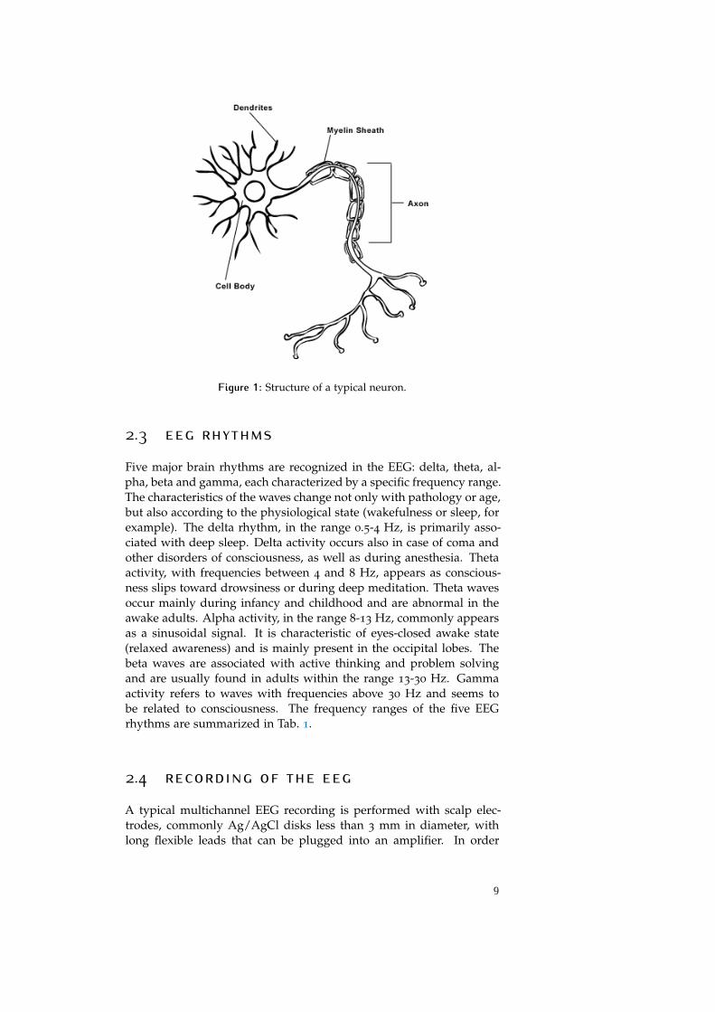
Figure 1: Structure of a typical neuron.
2.3 eeg rhythms
Five major brain rhythms are recognized in the EEG: delta, theta, al-pha, beta and gamma, each characterized by a specific frequency range.The characteristics of the waves change not only with pathology or age,but also according to the physiological state (wakefulness or sleep, forexample). The delta rhythm, in the range 0.5-4 Hz, is primarily asso-ciated with deep sleep. Delta activity occurs also in case of coma andother disorders of consciousness, as well as during anesthesia. Thetaactivity, with frequencies between 4 and 8 Hz, appears as conscious-ness slips toward drowsiness or during deep meditation. Theta wavesoccur mainly during infancy and childhood and are abnormal in theawake adults. Alpha activity, in the range 8-13 Hz, commonly appearsas a sinusoidal signal. It is characteristic of eyes-closed awake state(relaxed awareness) and is mainly present in the occipital lobes. Thebeta waves are associated with active thinking and problem solvingand are usually found in adults within the range 13-30 Hz. Gammaactivity refers to waves with frequencies above 30 Hz and seems tobe related to consciousness. The frequency ranges of the five EEGrhythms are summarized in Tab. 1.
2.4 recording of the eeg
A typical multichannel EEG recording is performed with scalp elec-trodes, commonly Ag/AgCl disks less than 3 mm in diameter, withlong flexible leads that can be plugged into an amplifier. In order
9
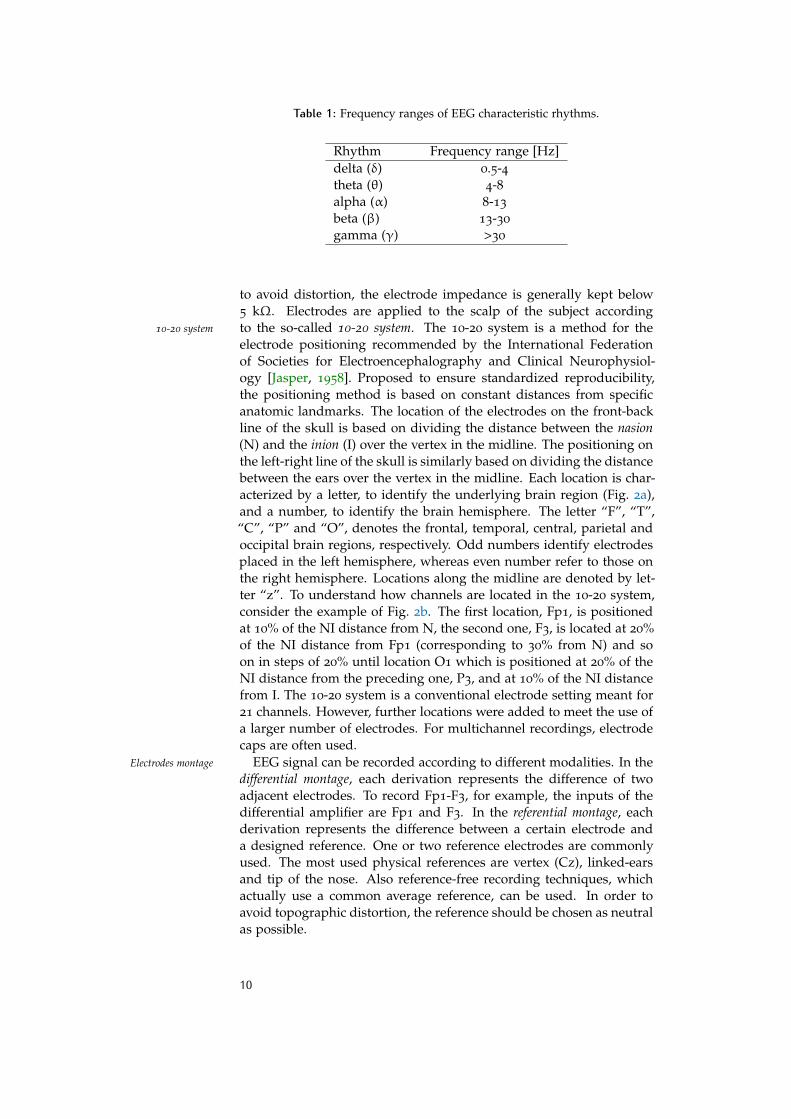
Table 1: Frequency ranges of EEG characteristic rhythms.
Rhythm Frequency range [Hz]delta (δ) 0.5-4theta (θ) 4-8alpha (α) 8-13
beta (β) 13-30
gamma (γ) >30
to avoid distortion, the electrode impedance is generally kept below5 kΩ. Electrodes are applied to the scalp of the subject accordingto the so-called 10-20 system. The 10-20 system is a method for the10-20 system
electrode positioning recommended by the International Federationof Societies for Electroencephalography and Clinical Neurophysiol-ogy [Jasper, 1958]. Proposed to ensure standardized reproducibility,the positioning method is based on constant distances from specificanatomic landmarks. The location of the electrodes on the front-backline of the skull is based on dividing the distance between the nasion(N) and the inion (I) over the vertex in the midline. The positioning onthe left-right line of the skull is similarly based on dividing the distancebetween the ears over the vertex in the midline. Each location is char-acterized by a letter, to identify the underlying brain region (Fig. 2a),and a number, to identify the brain hemisphere. The letter “F”, “T”,“C”, “P” and “O”, denotes the frontal, temporal, central, parietal andoccipital brain regions, respectively. Odd numbers identify electrodesplaced in the left hemisphere, whereas even number refer to those onthe right hemisphere. Locations along the midline are denoted by let-ter “z”. To understand how channels are located in the 10-20 system,consider the example of Fig. 2b. The first location, Fp1, is positionedat 10% of the NI distance from N, the second one, F3, is located at 20%of the NI distance from Fp1 (corresponding to 30% from N) and soon in steps of 20% until location O1 which is positioned at 20% of theNI distance from the preceding one, P3, and at 10% of the NI distancefrom I. The 10-20 system is a conventional electrode setting meant for21 channels. However, further locations were added to meet the use ofa larger number of electrodes. For multichannel recordings, electrodecaps are often used.
EEG signal can be recorded according to different modalities. In theElectrodes montage
differential montage, each derivation represents the difference of twoadjacent electrodes. To record Fp1-F3, for example, the inputs of thedifferential amplifier are Fp1 and F3. In the referential montage, eachderivation represents the difference between a certain electrode anda designed reference. One or two reference electrodes are commonlyused. The most used physical references are vertex (Cz), linked-earsand tip of the nose. Also reference-free recording techniques, whichactually use a common average reference, can be used. In order toavoid topographic distortion, the reference should be chosen as neutralas possible.
10
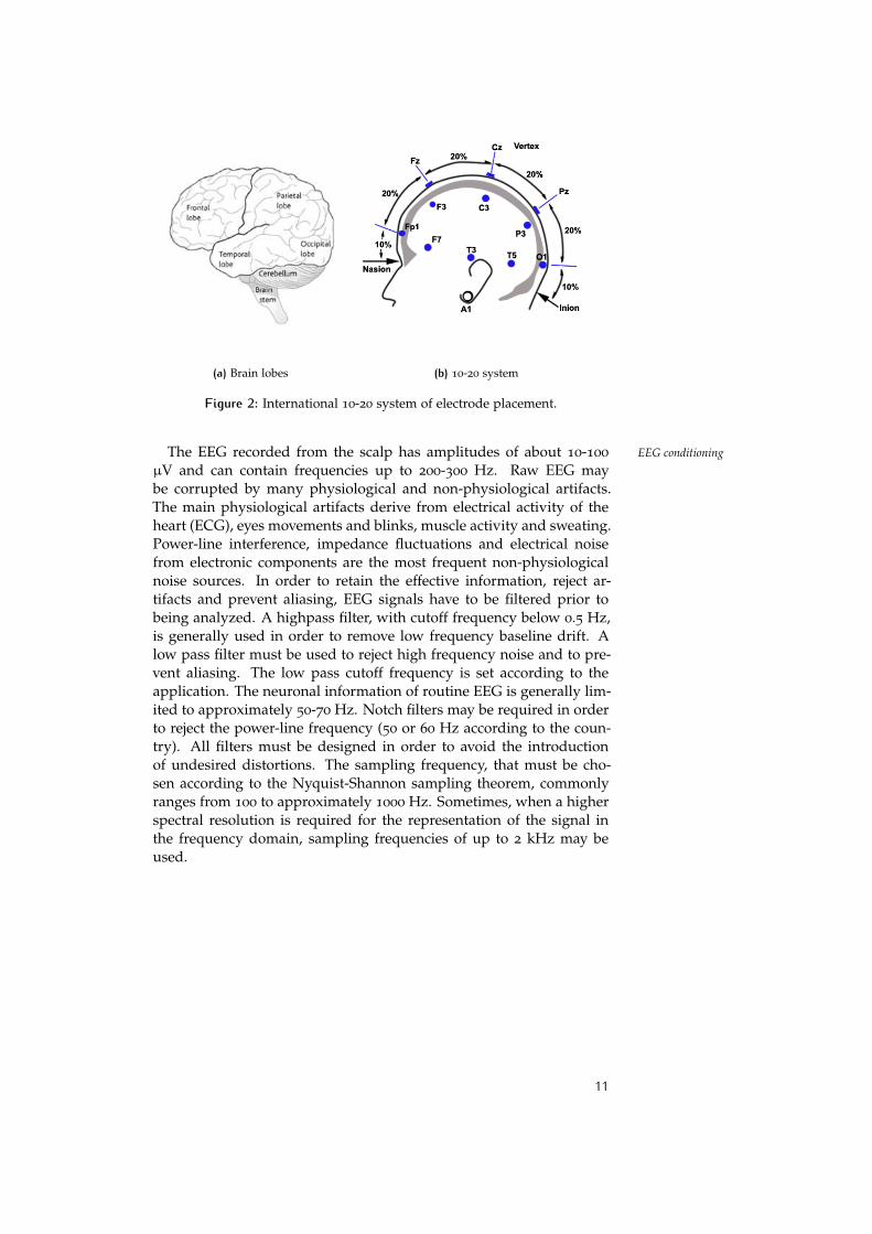
(a) Brain lobes (b) 10-20 system
Figure 2: International 10-20 system of electrode placement.
The EEG recorded from the scalp has amplitudes of about 10-100 EEG conditioning
µV and can contain frequencies up to 200-300 Hz. Raw EEG maybe corrupted by many physiological and non-physiological artifacts.The main physiological artifacts derive from electrical activity of theheart (ECG), eyes movements and blinks, muscle activity and sweating.Power-line interference, impedance fluctuations and electrical noisefrom electronic components are the most frequent non-physiologicalnoise sources. In order to retain the effective information, reject ar-tifacts and prevent aliasing, EEG signals have to be filtered prior tobeing analyzed. A highpass filter, with cutoff frequency below 0.5 Hz,is generally used in order to remove low frequency baseline drift. Alow pass filter must be used to reject high frequency noise and to pre-vent aliasing. The low pass cutoff frequency is set according to theapplication. The neuronal information of routine EEG is generally lim-ited to approximately 50-70 Hz. Notch filters may be required in orderto reject the power-line frequency (50 or 60 Hz according to the coun-try). All filters must be designed in order to avoid the introductionof undesired distortions. The sampling frequency, that must be cho-sen according to the Nyquist-Shannon sampling theorem, commonlyranges from 100 to approximately 1000 Hz. Sometimes, when a higherspectral resolution is required for the representation of the signal inthe frequency domain, sampling frequencies of up to 2 kHz may beused.
11

3 DY N A M I C A L S Y S T E M S A N DC H A O S T H E O R Y
contents3.1 Nonlinear dynamical systems 143.2 Phase space and attractors 143.3 Deterministic chaos and strange attractors 15
3.3.1 Sensitivity to initial conditions: Lyapunov exponents 16
3.3.2 Noninteger dimension: correlation dimension 16
3.4 Phase space reconstruction 173.4.1 Optimal m 18
3.4.2 Optimal τ 19
Since the early electroencephalographic recordings, the EEG mani-fested itself as an apparently random or aperiodic signal. The mostsimple system which produces aperiodic signals is a linear stochasticprocess. A stationary stochastic process can be described in the timedomain by mean and variance of the observed time series. A betterdescription, including the information about the time evolution of thesystem, is given by the so-called autocorrelation function, which mea-sures the linear correlation between data points. The same systemcan be equivalently approached using Fourier transform, a mathemati-cal tool which is used to decompose a signal into a set of sinusoidalcomponents whose amplitudes and phases are represented in the fre-quency domain. In the frequency domain the system is described bythe power spectral density which represents how the power of the sig-nal is distributed with frequency. The fruitful connection existing be-tween the autocorrelation function and the power spectral density isprovided by the Wiener-Khinchin theorem. The Wiener-Khinchin the-orem states that the power spectral density of a wide-sense stationarystochastic process is equal to the Fourier transform of the correspond-ing autocorrelation function. Hence, using Parseval’s theorem, the to-tal power of the signal can be calculated equivalently in the time or inthe frequency domain. If the system properties change over time, pro-ducing nonstationary signals, the short-time Fourier transform is used toproduce the spectrogram which provides a time-frequency represen-tation of the system. As many other aperiodic signals, the EEG hasbeen widely analyzed as the output of a stationary stochastic process.Traditional linear analysis of the EEG mainly involves the estimationof the power carried by the different rhythms characterizing the signal(Tab. 1).
The introduction of chaos theory provided a new approach to theanalysis of irregular time series. According to chaos theory, random be-havior can arise also in deterministic nonlinear dynamical system withjust a few dynamical variables. New methods were introduced to cap-
13
ture the unusual behavior of irregular time series, including the EEG.After a brief overview of nonlinear dynamical systems and their repre-sentation in the phase space, this chapter introduces the basics aboutchaos theory, including the concepts of unpredictability and strangeattractor. The measures for quantifying the properties of a chaoticsystem, including largest Lyapunov exponent and correlation dimen-sion are then presented. The chapter finally addresses the problem ofphase space reconstruction, which is required for the calculation of theaforementioned parameters. The notions provided in this chapter areadapted from Henry et al. [2001] and Kantz and Schreiber [2004].
3.1 nonlinear dynamical systemsThe concept of dynamical system is applied to any system that evolvesNonlinear dynamical
system in time. Dynamical systems evolving continuously in time are mathe-matically defined by a coupled set of first-order autonomous ordinarydifferential equations:
d
dtx(t) = F(x(t)) (1)
while a coupled set of first-order autonomous difference equations de-scribes dynamical systems whose behavior changes at discrete timeintervals:
xn+1 = G(xn) (2)
The components of the vectors x are the dynamical variables of thesystem evolving in continuous time (t ∈ R) or in discrete time (n ∈Z) and the components of the vector fields F and G represent thedynamical rules governing the evolution of the dynamical variables.The term autonomous refers to the property of the vector fields of beingnot explicitly dependent on time. It should be noted that there isno loss of generality in the restriction to autonomous systems sincea nonautonomous systems can be transformed into an autonomoussystems by the introduction of additional degrees of freedom.
Under modest smoothness assumptions about the evolution rules,Deterministicnonlinear dynamical
systemthe mathematical theory of ordinary differential (or difference) equa-tions ensures the existence of unique solutions. Thus, the dynamicalsystem is deterministic, that is, once the current state is determined,the state at any future time is determined as well. However, despitethe existence of unique solutions, there may be no explicit algebraicrepresentation of the state of the system at a given point in time.
3.2 phase space and attractorsPhase space is an abstract mathematical space in which each possi-Phase space
14

ble state of a dynamical system is represented by a point. Thus, ifthe systems is defined by a set of n first-order autonomous ordinarydifferential (or difference) equations, then the phase space is a finite di-mensional vector space in Rn. A sequence of points xn or x(t) solving Trajectory
the equations is a trajectory of the dynamical system in the phase space.As dynamical variables evolve in time, the representative point of xnand x(t) traces out a continuous curve or a sequence of points in thephase space, respectively. As time proceeds, trajectories in the phasespace can run away to infinity or remain in a bounded area. If a dy-namical system is also dissipative, that is, on average the phase spacevolume contracts as the system evolves, a set of initial conditions willbe attracted to some sub-set of the phase space. This sub-set, invari- Attractor
ant under the dynamical evolution, is called the attractor of the system.Simple examples of attractors are fixed points and limit cycles.
3.3 deterministic chaos and strange at-tractors
The solutions of many nonlinear dynamical systems are apparentlyrandom. Even though these systems are deterministic, with no ran-dom elements involved, they result highly unpredictable. However,random signals generated by noise are fundamentally different fromthose generated by low order deterministic dynamics. The behavior Deterministic chaos
of such systems, highly sensitive to initial conditions, is known as de-terministic chaos. Geometrical counterpart of the sensitivity to initialconditions is the complex structure exhibited by the attractors. These Strange attractors
attractors are known as strange attractors.One of the first examples of three-dimensional nonlinear dynamical
system evolving continuously in time and showing chaotic behavior isthe Lorenz oscillator [Lorenz, 1963]. The Lorenz oscillator is governedby the following differential equations:
dxdt = σ(y− x)dydt = x(ρ− z) − ydzdt = xy−βz
(3)
Figure 3a shows Lorenz strange attractor for ρ = 28, σ = 10 and β = 83 .
A two-dimensional discrete dynamical system is the Hénon map[Hénon, 1976]. The difference equations that describe the Hénon mapare:
xn+1 = yn + 1− ax2nyn+1 = bxn
(4)
The strange attractor of the canonical Hénon map, built with a = 1.4and b = 0.3, is shown in Fig 3b.
A strange attractor is characterized by the following properties:
15
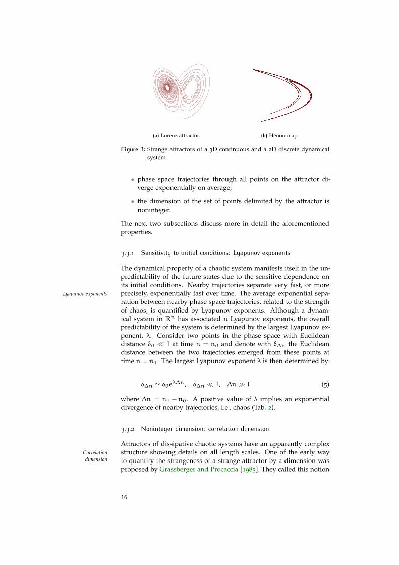
(a) Lorenz attractor. (b) Hénon map.
Figure 3: Strange attractors of a 3D continuous and a 2D discrete dynamicalsystem.
• phase space trajectories through all points on the attractor di-verge exponentially on average;
• the dimension of the set of points delimited by the attractor isnoninteger.
The next two subsections discuss more in detail the aforementionedproperties.
3.3.1 Sensitivity to initial conditions: Lyapunov exponents
The dynamical property of a chaotic system manifests itself in the un-predictability of the future states due to the sensitive dependence onits initial conditions. Nearby trajectories separate very fast, or moreprecisely, exponentially fast over time. The average exponential sepa-Lyapunov exponents
ration between nearby phase space trajectories, related to the strengthof chaos, is quantified by Lyapunov exponents. Although a dynam-ical system in Rn has associated n Lyapunov exponents, the overallpredictability of the system is determined by the largest Lyapunov ex-ponent, λ. Consider two points in the phase space with Euclideandistance δ0 1 at time n = n0 and denote with δ∆n the Euclideandistance between the two trajectories emerged from these points attime n = n1. The largest Lyapunov exponent λ is then determined by:
δ∆n ' δ0eλ∆n, δ∆n 1, ∆n 1 (5)
where ∆n = n1 − n0. A positive value of λ implies an exponentialdivergence of nearby trajectories, i.e., chaos (Tab. 2).
3.3.2 Noninteger dimension: correlation dimension
Attractors of dissipative chaotic systems have an apparently complexstructure showing details on all length scales. One of the early wayCorrelation
dimension to quantify the strangeness of a strange attractor by a dimension wasproposed by Grassberger and Procaccia [1983]. They called this notion
16
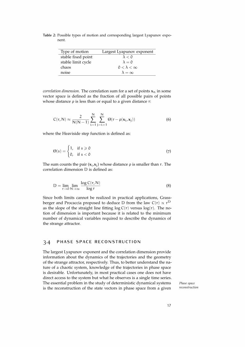
Table 2: Possible types of motion and corresponding largest Lyapunov expo-nent.
Type of motion Largest Lyapunov exponentstable fixed point λ < 0
stable limit cycle λ = 0
chaos 0 < λ <∞noise λ =∞
correlation dimension. The correlation sum for a set of points xn in somevector space is defined as the fraction of all possible pairs of pointswhose distance ρ is less than or equal to a given distance r:
C(r,N) ≈ 2
N(N− 1)
N∑i=1
N∑j=i+1
Θ(r− ρ(xi, xj)) (6)
where the Heaviside step function is defined as:
Θ(s) =
1, if s > 00, if s < 0
(7)
The sum counts the pair (xi,xj) whose distance ρ is smaller than r. Thecorrelation dimension D is defined as:
D = limr→0
limN→∞ logC(r,N)
log r(8)
Since both limits cannot be realized in practical applications, Grass-berger and Procaccia proposed to deduce D from the law C(r) ∝ rDas the slope of the straight line fitting logC(r) versus log(r). The no-tion of dimension is important because it is related to the minimumnumber of dynamical variables required to describe the dynamics ofthe strange attractor.
3.4 phase space reconstructionThe largest Lyapunov exponent and the correlation dimension provideinformation about the dynamics of the trajectories and the geometryof the strange attractor, respectively. Thus, to better understand the na-ture of a chaotic system, knowledge of the trajectories in phase spaceis desirable. Unfortunately, in most practical cases one does not havedirect access to the system but what he observes is a single time series.The essential problem in the study of deterministic dynamical systems Phase space
reconstructionis the reconstruction of the state vectors in phase space from a given
17
observation in time. The method of phase space reconstruction, de-veloped by Packard et al. [1980], has been rigorously justified by theembedding theorems of Takens [1981] and Sauer et al. [1994].
According to Takens, if the observed time series is one component ofEmbedding theorem
an attractor that can be represented by a smooth d-dimensional mani-fold (with d an integer) then the topological properties of the attractor(such as the largest Lyapunov exponent and the correlation dimension)are equivalent to the topological properties of the embedding formedby the m-dimensional phase space vectors:
sn = (sn−(m−1)τ, sn−(m−2)τ, ..., sn−τ, sn) (9)
whenever m > 2d + 1. In Eq. 9 τ is the time delay and m is theembedding dimension. Sauer extended Takens’ theorem to the case ofstrange attractors with noninteger dimension D.
To optimize the measurements of the largest Lyapunov exponentand the correlation dimension, there is the need to specify the opti-mum value for the embedding dimension m and the time delay τ.Although for many practical purposes the most important embeddingparameter is the product mτ, the embedding dimension and the timedelay are commonly chosen separately.
3.4.1 Optimal m
The main problem of phase space reconstruction is the choice of theEmbeddingdimension optimal embedding dimension. As asserted by the aforementioned
embedding theorems, a phase space is correctly reconstructed if theembedding dimension is chosen as m > 2D + 1. In this terms, if am embedding dimension provides a good representation of the phasespace, every m’ embedding dimension greater than m would be asmuch correct. However, the choice of an arbitrary large m value willresult in an increased computational effort required by the algorithmsfor the analysis of the dynamical system. Thus, the main problemin phase space reconstruction is the choice of the optimal embeddingdimension.
Kennel et al. [1992] developed a method for determining the em-False nearestneighbors bedding dimension introducing the concept of false nearest neighbors.
Consider two neighboring states in the phase space at a given time.Under smoothness assumptions about the dynamical rules governingthe system, the two trajectories emerging from the two points shouldbe still close after a short time interval δn despite the sensitivity toinitial conditions. If two neighboring states in a mi-dimensional spacediverge exponentially in the mi+1-dimensional space, then they aredefined “false neighbors” for the chosen mi embedding dimension.The algorithm compares the distances between neighboring trajecto-ries at successively higher dimensions. When the ratio between thedistances in dimension mi and in dimension mi+1 is greater than afixed threshold, large enough to allow for exponential divergence due
18

to deterministic chaos, then the considered trajectories are false neigh-bors. As i increases, the percentage r of false neighbors decreases andthe optimal embedding dimension is chosen where r approaches zero.
3.4.2 Optimal τ
The embedding theorems consider data with infinite precision. Thus, Time delay
embedding with the same dimension m but different time delay τ areequivalent in the mathematical sense for noise-free data. However, if τis small compared to the internal time scales of the system, consecutivephase space points are strongly correlated. On the other hand, for largevalues of time delay successive elements are already almost indepen-dent. One of the most common methods for determining the optimal Autocorrelation
time delay is based on the behavior of the autocorrelation function ofthe signal. According to this method, the first zero of the autocorrela-tion function represents a good value of τ. Another proposal is based Mutual information
on the more refined concept of mutual information introduced by Fraserand Swinney [1986]. The optimal value of time delay corresponds tothe first local minimum of the mutual information which is a quantitythat measures how much information on the average can be predictedabout one time series point given full information about the other.
19

4 F R A C TA L G E O M E T R Y O FT H E E E G
contents4.1 Fractals and self-similarity 214.2 Self-similarity and dimension 224.3 Time-domain self-similarity 254.4 Fractional Brownian motion 254.5 Self-affinity 264.6 Statistical self-affinity: fractal dimension, Hurst index and β
exponent 274.7 Modeling EEG with fBm 294.8 Time domain fractal approach 29
The measures presented in the preceding chapter for the character-ization of a dynamical system producing irregular time series requirethe reconstruction of the phase space, a procedure which may be com-putationally expensive.
A new perspective to approach the study of such systems withoutreconstructing the attractor is offered by the concept of fractal geome-try. Complexity is a theme shared by many physiological systems inall areas of medical research. The classical notion of scaling is not ableto describe the irregular structures seen in lungs and brain, as well asthe irregular patterns of electroencephalographic and heart rate vari-ability signals. In this chapter, the main features of fractal shapes arefirstly presented in the more intuitive space domain and then adaptedfor the characterization of fractal processes in time. Fractional Brow-nian motion, the most used mathematical model for natural fractalprocesses, including the EEG, is then described. Finally, the fractal ap-proach adopted by the Author during the PhD course for the analysisof the EEG is presented. The theoretical concepts presented in thischapter are adapted from Peitgen and Saupe [1988].
4.1 fractals and self-similarityWithin the last 30 years fractal geometry has become a central con-cept in most of the natural sciences, among which physics, chemistry,physiology and meteorology. Although fractal objects are complex inappearance, they arise from simple rules and contrarily to Euclideanshapes, they represent more suitable models for natural phenomena.
To understand the major differences between Euclidean and frac- Euclidean versusfractal geometrytal geometry, consider a three-dimensional Euclidean shape, for exam-
ple a sphere. A sphere is characterized by one size (the radius r), is
21
completely described by a simple algebraic formula ((x− x0)2 + (y−
y0)2 + (z− z0)
2 = r2) and provides an accurate description of manyartificial objects. Fractals, on the contrary, have no characteristic size(they are self-similar or independent of scale), are usually the result ofa recursive construction procedure and provide a good description ofmany natural shapes, processes or phenomena (coastlines, turbulence,snowflakes, etc.).
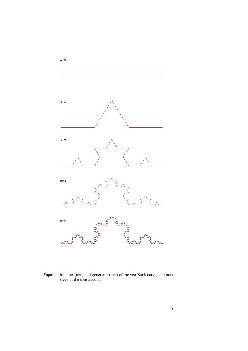
Consider the von Koch curve, one of the first mathematical fractalsdescribed in literature [von Koch, 1904]. Figure 4 shows the first foursteps of the recursive procedure for constructing this famous fractalcurve. A line segment is first divided into three equal segments (n=0).The middle segment is replaced by two equal segments forming twosides of an equilateral triangle (n=1). This procedure is then repeatedon each of the four segments, whose middle third is replaced by twoequal segments forming two sides of an equilateral triangle (n=2). Oneach iteration, the number of the segments is multiplied by four whilethe length of the segments is divided by three. Thus, the length ofthe curve increases by a factor of 43 with each iteration. The von Kochcurve is the limiting curve obtained by iterating the construction rulean infinite number of times.
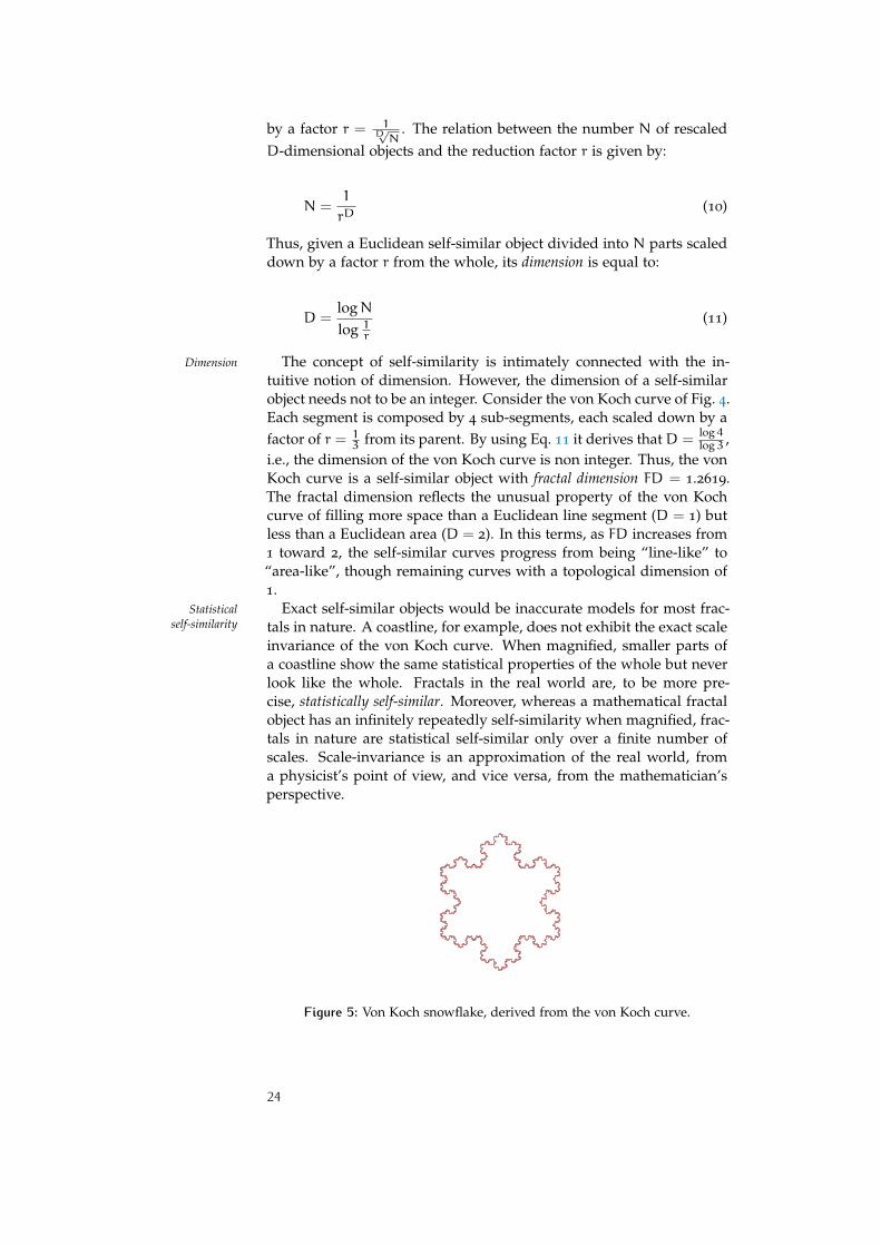
The von Koch curve has no characteristic size. It exhibits an exactself-similarity, meaning that each small portion, when magnified, is ex-actly identical to the original one. The curve is said to be independentof scale because there will be an equivalent level of detail at every scale.Moreover, the limiting curve obtained after an infinite number of iter-ations would compress an infinite length into a finite area of the planewithout intersecting itself. The von Koch curve, though apparentlycomplex, is produced by the iteration of a very simple rule. However,there is no algebraic formula that can describe its points in the plane.Based on the von Koch curve, the fractal shape of Fig. 5 provides agood description of the snowflake.
4.2 self-similarity and dimension
One of the central concepts of fractal geometry is the property of self-Self-similarity
similarity, also known as scaling or scale-invariance. Although everyfractal exhibits some form of self-similarity, it is not true that, if anobject is self-similar, then it is fractal. Consider a one-dimensional Eu-clidean object like a line segment. It can be divided into N identicalsegments each reduced by a scaling factor r = 1
N . A two-dimensionalEuclidean object, for example a square area, can be divided into Nsmaller squares, each scaled down by a factor r = 1
2√N
. Similarly, athree-dimensional Euclidean object, such as a solid cube, can be di-vided into N self-similar copies, each scaled down by a factor r = 1
3√N
.It can be deduced that, in the same way, a D-dimensional self-similarobject can be divided into N identical parts each of which is reduced
22
n=0
n=1
n=2
n=3
n=4
Figure 4: Initiator (n=0) and generator (n=1) of the von Koch curve, and nextsteps in the construction.
23
by a factor r = 1D√N
. The relation between the number N of rescaledD-dimensional objects and the reduction factor r is given by:
N =1
rD(10)
Thus, given a Euclidean self-similar object divided into N parts scaleddown by a factor r from the whole, its dimension is equal to:
D =logNlog 1r
(11)
The concept of self-similarity is intimately connected with the in-Dimension
tuitive notion of dimension. However, the dimension of a self-similarobject needs not to be an integer. Consider the von Koch curve of Fig. 4.Each segment is composed by 4 sub-segments, each scaled down by afactor of r = 1
3 from its parent. By using Eq. 11 it derives thatD =log4log3 ,
i.e., the dimension of the von Koch curve is non integer. Thus, the vonKoch curve is a self-similar object with fractal dimension FD = 1.2619.The fractal dimension reflects the unusual property of the von Kochcurve of filling more space than a Euclidean line segment (D = 1) butless than a Euclidean area (D = 2). In this terms, as FD increases from1 toward 2, the self-similar curves progress from being “line-like” to“area-like”, though remaining curves with a topological dimension of1.
Exact self-similar objects would be inaccurate models for most frac-Statisticalself-similarity tals in nature. A coastline, for example, does not exhibit the exact scale
invariance of the von Koch curve. When magnified, smaller parts ofa coastline show the same statistical properties of the whole but neverlook like the whole. Fractals in the real world are, to be more pre-cise, statistically self-similar. Moreover, whereas a mathematical fractalobject has an infinitely repeatedly self-similarity when magnified, frac-tals in nature are statistical self-similar only over a finite number ofscales. Scale-invariance is an approximation of the real world, froma physicist’s point of view, and vice versa, from the mathematician’sperspective.
Figure 5: Von Koch snowflake, derived from the von Koch curve.
24
4.3 time-domain self-similarity
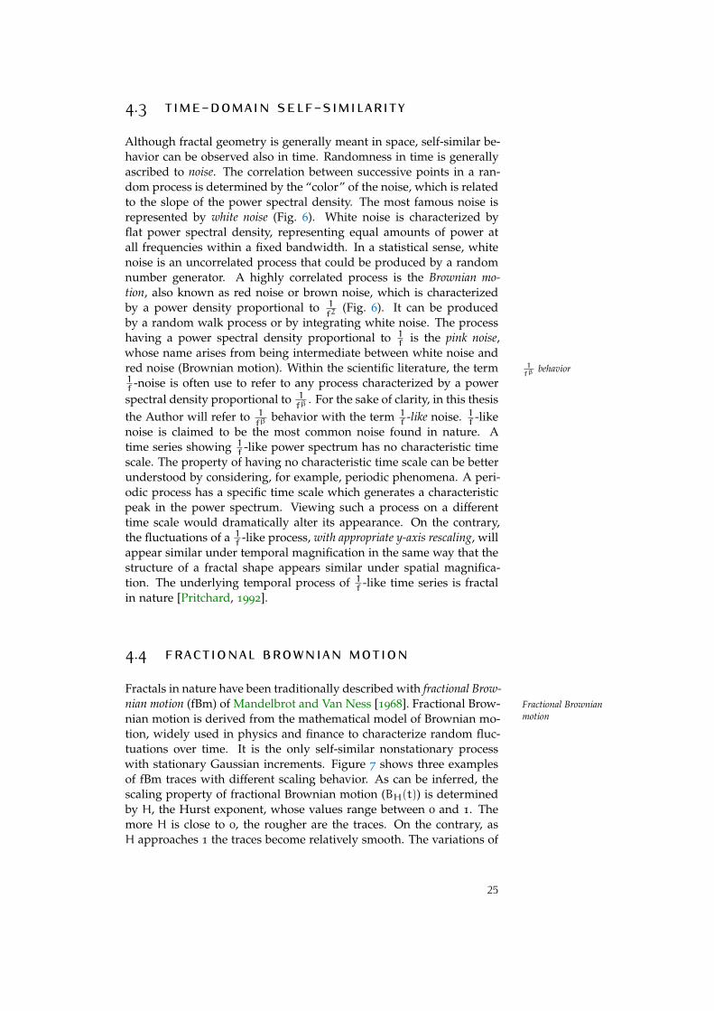
Although fractal geometry is generally meant in space, self-similar be-havior can be observed also in time. Randomness in time is generallyascribed to noise. The correlation between successive points in a ran-dom process is determined by the “color” of the noise, which is relatedto the slope of the power spectral density. The most famous noise isrepresented by white noise (Fig. 6). White noise is characterized byflat power spectral density, representing equal amounts of power atall frequencies within a fixed bandwidth. In a statistical sense, whitenoise is an uncorrelated process that could be produced by a randomnumber generator. A highly correlated process is the Brownian mo-tion, also known as red noise or brown noise, which is characterizedby a power density proportional to 1
f2(Fig. 6). It can be produced
by a random walk process or by integrating white noise. The processhaving a power spectral density proportional to 1
f is the pink noise,whose name arises from being intermediate between white noise andred noise (Brownian motion). Within the scientific literature, the term 1
fβbehavior
1f -noise is often use to refer to any process characterized by a powerspectral density proportional to 1
fβ. For the sake of clarity, in this thesis
the Author will refer to 1fβ
behavior with the term 1f -like noise. 1f -like
noise is claimed to be the most common noise found in nature. Atime series showing 1
f -like power spectrum has no characteristic timescale. The property of having no characteristic time scale can be betterunderstood by considering, for example, periodic phenomena. A peri-odic process has a specific time scale which generates a characteristicpeak in the power spectrum. Viewing such a process on a differenttime scale would dramatically alter its appearance. On the contrary,the fluctuations of a 1f -like process, with appropriate y-axis rescaling, willappear similar under temporal magnification in the same way that thestructure of a fractal shape appears similar under spatial magnifica-tion. The underlying temporal process of 1f -like time series is fractalin nature [Pritchard, 1992].
4.4 fractional brownian motion
Fractals in nature have been traditionally described with fractional Brow-nian motion (fBm) of Mandelbrot and Van Ness [1968]. Fractional Brow- Fractional Brownian
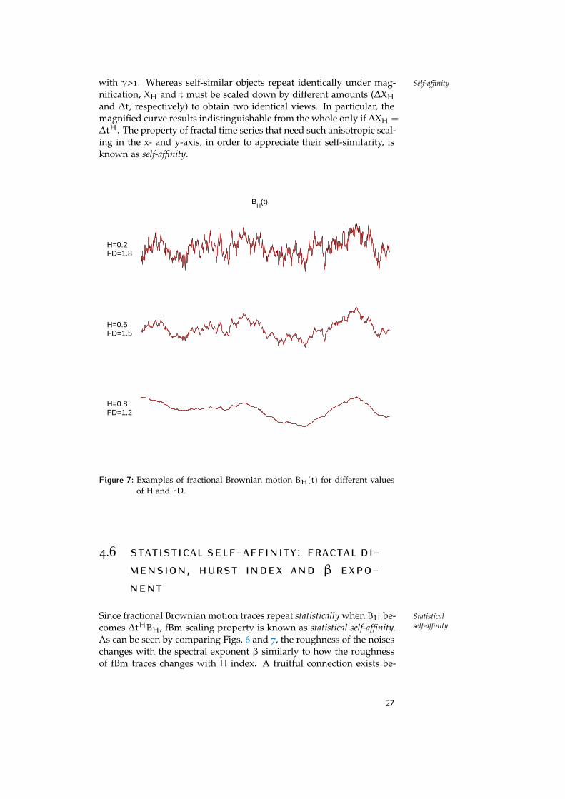
motionnian motion is derived from the mathematical model of Brownian mo-tion, widely used in physics and finance to characterize random fluc-tuations over time. It is the only self-similar nonstationary processwith stationary Gaussian increments. Figure 7 shows three examplesof fBm traces with different scaling behavior. As can be inferred, thescaling property of fractional Brownian motion (BH(t)) is determinedby H, the Hurst exponent, whose values range between 0 and 1. Themore H is close to 0, the rougher are the traces. On the contrary, asH approaches 1 the traces become relatively smooth. The variations of
25
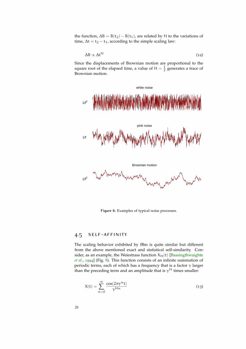
the function, ∆B = B(t2) − B(t1), are related by H to the variations oftime, ∆t = t2 − t1, according to the simple scaling law:
∆B ∝ ∆tH (12)
Since the displacements of Brownian motion are proportional to thesquare root of the elapsed time, a value of H = 1
2 generates a trace ofBrownian motion.
Brownian motion
pink noise
white noise
1/f0
1/f
1/f2
Figure 6: Examples of typical noise processes.
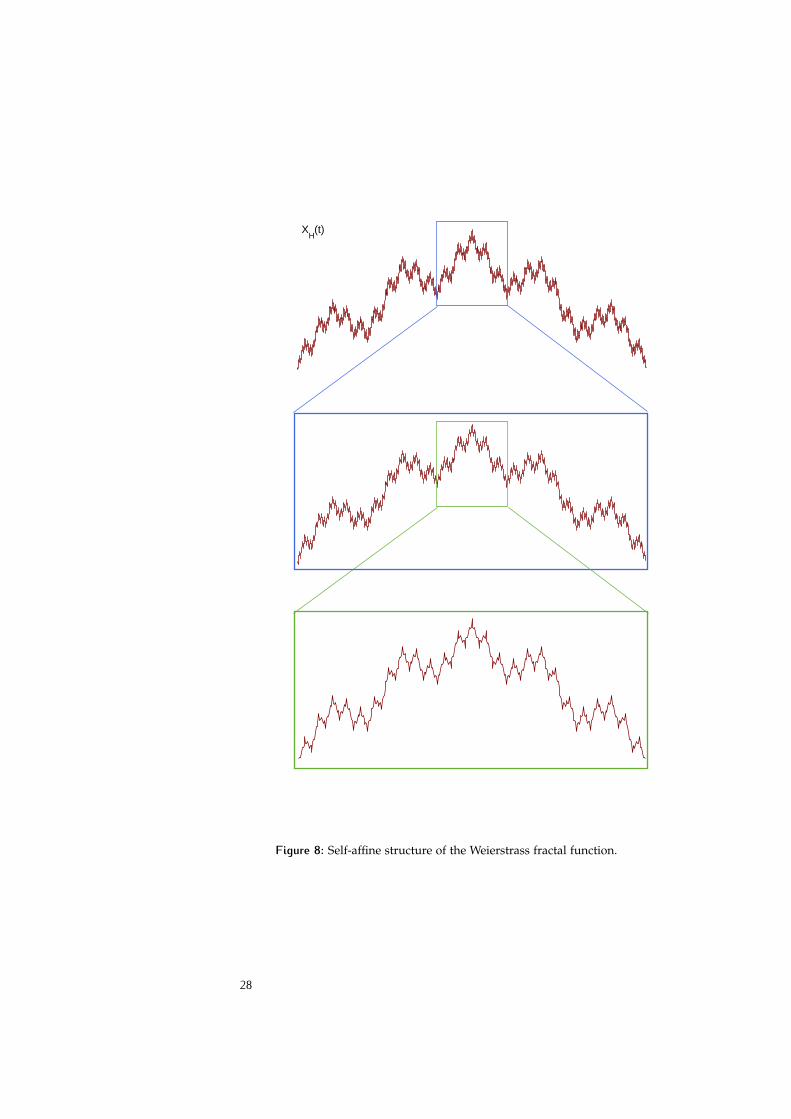
4.5 self-affinityThe scaling behavior exhibited by fBm is quite similar but differentfrom the above mentioned exact and statistical self-similarity. Con-sider, as an example, the Weiestrass function XH(t) [Bassingthwaighteet al., 1994] (Fig. 8). This function consists of an infinite summation ofperiodic terms, each of which has a frequency that is a factor γ largerthan the preceding term and an amplitude that is γH times smaller:
X(t) =
∞∑n=0
cos(2πγnt)γHn
(13)
26
with γ>1. Whereas self-similar objects repeat identically under mag- Self-affinity
nification, XH and t must be scaled down by different amounts (∆XHand ∆t, respectively) to obtain two identical views. In particular, themagnified curve results indistinguishable from the whole only if ∆XH =
∆tH. The property of fractal time series that need such anisotropic scal-ing in the x- and y-axis, in order to appreciate their self-similarity, isknown as self-affinity.
H=0.2FD=1.8
H=0.5FD=1.5
H=0.8FD=1.2
BH(t)
Figure 7: Examples of fractional Brownian motion BH(t) for different valuesof H and FD.
4.6 statistical self-affinity: fractal di-mension, hurst index and β expo-nent
Since fractional Brownian motion traces repeat statistically when BH be- Statisticalself-affinitycomes ∆tHBH, fBm scaling property is known as statistical self-affinity.
As can be seen by comparing Figs. 6 and 7, the roughness of the noiseschanges with the spectral exponent β similarly to how the roughnessof fBm traces changes with H index. A fruitful connection exists be-
27
XH(t)
Figure 8: Self-affine structure of the Weierstrass fractal function.
28
tween the three equivalent characterization FD, H and β of a fBm func-tion:
FD = 2−H =5−β
2(14)
For H ∈ (0,1), FD is in the range 1-2 and 1 < β < 3.
4.7 modeling eeg with fbm
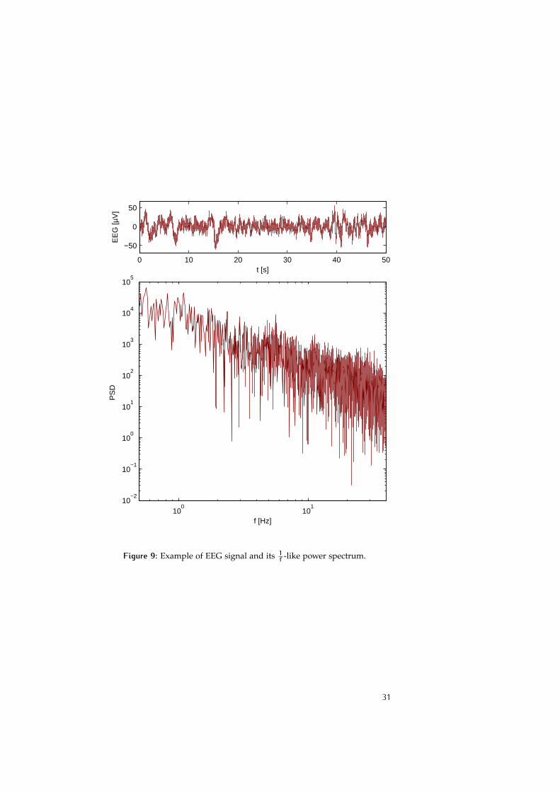
The so-called 1f -like behavior is a ubiquitous property of complex bio-
logical systems. In such scaling, the power spectral density of a timeseries is governed by an inverse power-law:
PSD ∝ 1
fβ(15)
where the exponent β is related to the color of the series, that is, tothe degree of autocorrelation. The human EEG reflects the ongoingactivity of the underlying complex system: the human brain. In oneof the first studies on the fractal-like behavior of the EEG, Pritchard[1992] reported that the EEG exhibits significant 1f -like power scaling,suggesting that the human brain is fractal in time. Moreover, he ob-served that the EEG displays “more color” than a truly 1
f process,meaning that the EEG is autocorrelated to a greater degree. The par-ticular broad-band power spectrum of the EEG could be generated bya high dimensional stochastic system where a large number of multi-plicative subprocesses switch from log-normal to 1
f -like. However, theunpredictability of the EEG could also be attributed to the sensitive de-pendence on initial conditions of a low dimensional system governedby deterministic chaos and described by a few nonlinear differential(or difference) equations [Pritchard, 1992].
Although the origin of the 1f -like behavior of EEG power spectrumstill remains a mystery, the fractal analysis of the signal has become apowerful tool for the characterization of many physiological and patho-logical mechanisms involving complexity changes. Given the typical1fβ
power spectrum of the EEG (example in Fig. 22), with β in therange 1-3, fractional Brownian motion turned out to be the most suit-able mathematical model for its description. In these terms, EEG statis-tical self-affinity can be equivalently characterized by the three scalingparameters: the the Hurst index (H), the fractal dimension (FD) andthe power-law exponent (β).
4.8 time domain fractal approachThe study of the fractal-like behavior of the EEG can be approachedboth in the time-domain and in the frequency-domain. In this the-sis the attention is focused on the time-domain analysis, i.e., on the
29

characterization of the EEG in terms of fractal dimension, to meet thegrowing need for real-time systems. Several methods have been pro-Fractal dimension
posed to estimate the fractal dimension of a time series. One of theearly techniques for calculating the fractal dimension of a waveform isthe box-counting method [Mandelbrot, 1982], based on counting howmany 2D cells of size ε are required to cover the total length of thecurve. A similar method, based on the morphological covering of thecurve, was proposed by Maragos and Sun [1983]. Two of the most usedalgorithms were developed in the late ’80s by Higuchi [1988] and Katz[1988], the latter improved by Petrosian [1995] to reduce the executiontime. More recently, Sevcik [2006] and Paramanathan and Uthayaku-mar [2008] proposed new procedures to estimate the fractal dimensionof waveforms.
In order to identify the most accurate and reliable algorithm, theAlgorithms for directestimation Author firstly selected three of the most used methods for the esti-
mation of EEG fractal dimension: the box-counting method, Katz’salgorithm and Higuchi’s algorithm. The algorithms were then com-pared by evaluating not only the ability to provide accurate estimatesbut also their sensitivity to parameters like the sampling frequency ofthe EEG and the estimation time window length. The results of thisresearch, presented in Chapter 5, are guidelines that will be appliedto the experimental investigations presented in Part II for the correctfractal analysis of the EEG.
Despite the plethora of algorithms available for the fractal analysisfBm model forindirect estimation of the EEG directly in the time domain, the use of the relationship 14
to derive FD from the calculated β exponent is widespread amongphysicians. Conversely, sometimes the scaling exponent β is obtainedfrom the fractal dimension estimated in the time-domain to describethe power-law of the EEG. The accuracy of the estimates obtained bythe application of Eq. 14 relies on the accuracy of the fBm model. Atpresent, a detailed model of the system that generates the EEG is farfrom being feasible. Deviations from 1
f -like behavior may occur moreoften than thought, not only owing to abnormalities introduced bypathological states. Pritchard [1992], for example, observed that devi-ations from log-log linearity are associated with the eyes-closed alpharhythm in resting state EEG. From this perspective, the values obtainedusing the scaling relationship 14 may be inaccurate estimates of thereal parameters. A further research carried out during the PhD course,aimed at empirically verifying the relationship existing between FD
and β to establish how much the EEG deviates from fBm, is presentedin Chapter 6.
30
0 10 20 30 40 50
−50
0
50
t [s]
EE
G [µ
V]
100
101
10−2
10−1
100
101
102
103
104
105
f [Hz]
PS
D
Figure 9: Example of EEG signal and its 1f -like power spectrum.
31

5 F R A C TA L D I M E N S I O NE S T I M AT I O N A LG O R I T H M S
contents5.1 Introduction and motivation 335.2 Materials and Methods 35
5.2.1 Fractal dimension estimation algorithms 35
5.2.2 Synthetic series analysis 37
5.2.3 EEG analysis 39
5.3 Results 415.3.1 Results on synthetic series 41
5.3.2 Results on the EEG 44
5.4 Discussion 485.5 Conclusion 49
This chapter provides the description of three algorithms widelyused for the estimation of the fractal dimension of waveforms: the box-counting method [Mandelbrot, 1982], Katz’s algorithm [Katz, 1988]and Higuchi’s algorithm [Higuchi, 1988]. The performances of theaforementioned algorithms are compared in terms of accuracy, sensi-tivity to the sampling frequency and dependence on the estimationtime window length. Aim of the study is the identification of the mostreliable algorithm to be applied for the fractal analysis of the EEG. Theinvestigation is performed in two steps: the algorithms are firstly ap-plied to three synthetic series of known fractal dimension and thenused for the analysis of EEG traces acquired from twenty full-termsleeping newborns. The chapter is based on Author’s publications 2
and 4.
5.1 introduction and motivationAs mentioned in Chapter 4, the complexity of many physiological sys-tems can be assessed through the analysis of the irregular time seriesthey generate. Such time series, apparently random or aperiodic intime, are frequently independent of scale and self-similar under mag-nification [Mandelbrot, 1982]. The particular non-uniform scaling of atime series which is invariant under a transformation that scales differ-ent coordinates by different amounts is known as self-affinity [Mandel-brot, 1985]. Self-affine time series are characterized, in the frequencydomain, by a power-law spectrum. Among the plethora of indexesthat can describe the irregularity of waveforms showing self-affinity intime and power-law spectrum, the fractal dimension (FD) has gainedwide acceptance.
33
The electroencephalogram is a fractal-like signal whose underlyingmechanisms reflect the complexity of brain activity [Acharya et al.,2005; Bosl et al., 2011; Catarino et al., 2011; Chouvarda et al., 2011;Mizuno et al., 2010]. For this reason it represents a rich source ofinformation about several pathophysiological phenomena. The frac-tal dimension, for example, is a powerful EEG index in the monitor-ing of the depth of anesthesia [Ferenets et al., 2006, 2007] as well asin the identification of wake/drowsy states [Bojic et al., 2010; Inouyeet al., 1994] and of different sleep stages [Acharya et al., 2005; Car-rozzi et al., 2004; Chouvarda et al., 2011]. It also represents a usefulparameter for the characterization of psychiatric brain diseases likeschizophrenia [Raghavendra et al., 2009] and autism [Ahmadlou et al.,2010], for the diagnosis and monitoring of neurological disorders likeAlzheimer’s disease [Ahmadlou et al., 2011] and for epileptic seizuredetection and prediction [Accardo et al., 1997; Daneshyari et al., 2010;Polychronaki et al., 2010].
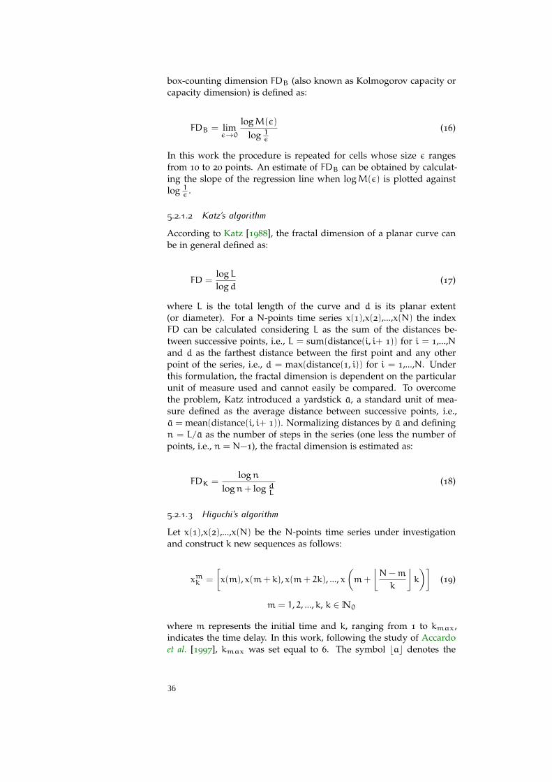
The practice of obtaining FD estimates from spectral analysis by us-ing the scaling relationship derived from Eq. 14, i.e., FD = (5−β)/2,with β representing the exponent of the power-law, is widespread[Phothisonothai and Nakagawa, 2009; Rankine et al., 2007]. However,many methods have been proposed in order to estimate the fractal di-mension of waveforms directly in the time-domain, allowing the analy-sis of biological events also of brief duration [Higuchi, 1988; Katz, 1988;Paramanathan and Uthayakumar, 2008; Petrosian, 1995].
Although some comparison studies [Accardo et al., 1997; Estelleret al., 2001; Paramanathan and Uthayakumar, 2008; Raghavendra andDutt, 2009] have demonstrated that Higuchi’s algorithm [Higuchi, 1988]is the most accurate in estimating the fractal dimension of waveforms,other techniques, like box-counting method [Mandelbrot, 1982] andKatz’s algorithm [Katz, 1988], have often been used to calculate EEGfractal dimension. Moreover, regardless of the chosen algorithm, noenough attention has been paid on the possible influence of the sig-nal sampling frequency and the estimation time window length on FDvalues.
As regard the sampling frequency, EEG traces are commonly ac-quired at various rates ranging from about 100 Hz to 1024 Hz or higher.Sometimes, especially to increase frequency resolution in spectral anal-ysis, EEG signals are oversampled. Generally the oversampling doesnot affect visual or traditional linear analysis of the EEG, providedthat a suitable filtering has been used. As far as the time windowlength used for FD estimation, it is usually set according to the eventsto be analyzed and therefore it is also very variable. However, it isstill unclear if oversampling of different time windows could producesignificant changes in the fractal analysis, which is based on geometriccharacteristics of signals.
Raghavendra and Dutt [2009] compared the performances of Higu-State of the art
chi’s and Katz’s algorithms on four synthetic functions of known frac-tal dimension and on one EEG sleep trace, testing the sensitivity of theestimates to the sampling frequency only for one of the four synthetic
34
functions and for three values of fractal dimension. However, the sam-pling frequency of the synthetic functions was not set according tothe Nyquist-Shannon sampling theorem causing an undesired under-sampling. The study of Esteller et al. [2001] also compared the perfor-mances of Higuchi’s and Katz’s algorithms on one synthetic functionof known fractal dimension and on 16 intracranial EEGs of epilepticpatients. The effect of the estimation time window length was testedonly on the synthetic function. However, the window length incre-ment did not correspond to an effective time increment but rather to asampling frequency increment. Moreover, also in this case, the condi-tions of the Nyquist-Shannon sampling theorem were not fulfilled. Asimilar procedure, applied also on EEG signals, was followed in thestudy of Paramanathan and Uthayakumar [2008] for the comparisonof Higuchi’s and Katz’s algorithms.
In all the aforementioned studies the dependence of the algorithmson the time window length was not correctly assessed and the inves-tigation of their sensitivity to the sampling frequency could be invali-dated by an inappropriate sampling procedure.
In order to circumvent the problems that may arise from an incor- Algorithmscomparisonrect selection either of the length of the time window or of the sam-
pling frequency, in the present study a detailed comparison of threemethods commonly used for the estimation of EEG fractal dimension(the box-counting [Mandelbrot, 1982], the Katz’s [Katz, 1988] and theHiguchi’s [Higuchi, 1988] algorithms) was carried out at the appropri-ate sampling frequencies (greater than the Nyquist rate) and on dif-ferent time windows. The sensitivity to both the sampling frequencyand the time window length was evaluated for all algorithms. Thestudy was performed in two steps: the algorithms were at first testedon three synthetic functions of known fractal dimension for differentvalues of fractal dimension (FD), sampling frequency (FS) and timewindow length (TWL). In the second step, the results were comparedwith those achieved from the analysis of 20 neonatal EEGs for differentvalues of FS and TWL.
5.2 materials and methods
5.2.1 Fractal dimension estimation algorithms
5.2.1.1 Box-counting algorithm
One of the most common ways to measure the fractal dimension of atime series is the box-counting method [Mandelbrot, 1982]. It consistsin covering the waveform with small cells of size ε. If M(ε) denotesthe number of such cells required to cover the waveform, then the
35
box-counting dimension FDB (also known as Kolmogorov capacity orcapacity dimension) is defined as:
FDB = limε→0
logM(ε)
log 1ε(16)
In this work the procedure is repeated for cells whose size ε rangesfrom 10 to 20 points. An estimate of FDB can be obtained by calculat-ing the slope of the regression line when logM(ε) is plotted againstlog 1ε .
5.2.1.2 Katz’s algorithm
According to Katz [1988], the fractal dimension of a planar curve canbe in general defined as:
FD =logLlogd
(17)
where L is the total length of the curve and d is its planar extent(or diameter). For a N-points time series x(1),x(2),...,x(N) the indexFD can be calculated considering L as the sum of the distances be-tween successive points, i.e., L = sum(distance(i, i+ 1)) for i = 1,...,Nand d as the farthest distance between the first point and any otherpoint of the series, i.e., d = max(distance(1, i)) for i = 1,...,N. Underthis formulation, the fractal dimension is dependent on the particularunit of measure used and cannot easily be compared. To overcomethe problem, Katz introduced a yardstick a, a standard unit of mea-sure defined as the average distance between successive points, i.e.,a = mean(distance(i, i+ 1)). Normalizing distances by a and definingn = L/a as the number of steps in the series (one less the number ofpoints, i.e., n = N−1), the fractal dimension is estimated as:
FDK =logn
logn+ log dL(18)
5.2.1.3 Higuchi’s algorithm
Let x(1),x(2),...,x(N) be the N-points time series under investigationand construct k new sequences as follows:
xmk =
[x(m), x(m+ k), x(m+ 2k), ..., x
(m+
⌊N−m
k
⌋k
)](19)
m = 1, 2, ...,k, k ∈N0
where m represents the initial time and k, ranging from 1 to kmax,indicates the time delay. In this work, following the study of Accardoet al. [1997], kmax was set equal to 6. The symbol bac denotes the
36
integer part of a. For each xmk constructed series the length Lm(k) iscalculated as:
Lm(k) =
bN−m
k c∑i=1
|x(m+ ik) − x(m+ (i− 1)k)|
N− 1⌊N−mk
⌋k
1k
(20)
where the term
N−1
bN−mk ck
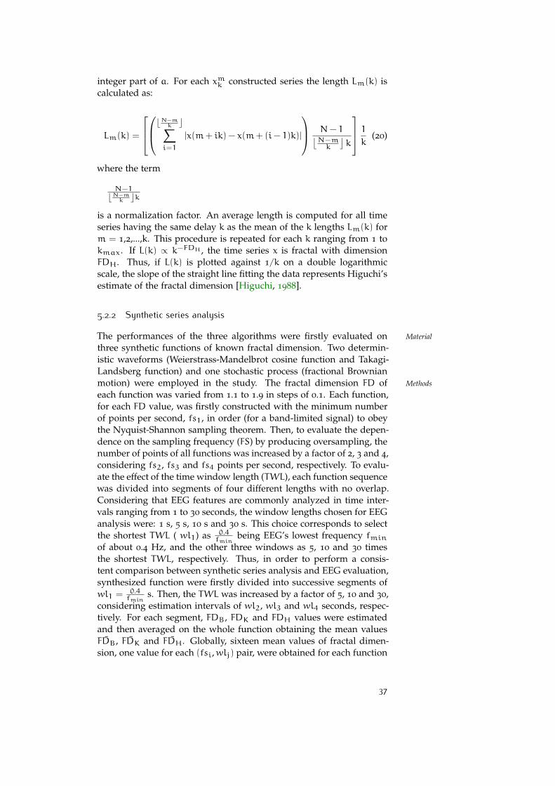
is a normalization factor. An average length is computed for all timeseries having the same delay k as the mean of the k lengths Lm(k) form = 1,2,...,k. This procedure is repeated for each k ranging from 1 tokmax. If L(k) ∝ k−FDH , the time series x is fractal with dimensionFDH. Thus, if L(k) is plotted against 1/k on a double logarithmicscale, the slope of the straight line fitting the data represents Higuchi’sestimate of the fractal dimension [Higuchi, 1988].
5.2.2 Synthetic series analysis
The performances of the three algorithms were firstly evaluated on Material
three synthetic functions of known fractal dimension. Two determin-istic waveforms (Weierstrass-Mandelbrot cosine function and Takagi-Landsberg function) and one stochastic process (fractional Brownianmotion) were employed in the study. The fractal dimension FD of Methods
each function was varied from 1.1 to 1.9 in steps of 0.1. Each function,for each FD value, was firstly constructed with the minimum numberof points per second, fs1, in order (for a band-limited signal) to obeythe Nyquist-Shannon sampling theorem. Then, to evaluate the depen-dence on the sampling frequency (FS) by producing oversampling, thenumber of points of all functions was increased by a factor of 2, 3 and 4,considering fs2, fs3 and fs4 points per second, respectively. To evalu-ate the effect of the time window length (TWL), each function sequencewas divided into segments of four different lengths with no overlap.Considering that EEG features are commonly analyzed in time inter-vals ranging from 1 to 30 seconds, the window lengths chosen for EEGanalysis were: 1 s, 5 s, 10 s and 30 s. This choice corresponds to selectthe shortest TWL ( wl1) as 0.4
fminbeing EEG’s lowest frequency fmin
of about 0.4 Hz, and the other three windows as 5, 10 and 30 timesthe shortest TWL, respectively. Thus, in order to perform a consis-tent comparison between synthetic series analysis and EEG evaluation,synthesized function were firstly divided into successive segments ofwl1 = 0.4
fmins. Then, the TWL was increased by a factor of 5, 10 and 30,
considering estimation intervals of wl2, wl3 and wl4 seconds, respec-tively. For each segment, FDB, FDK and FDH values were estimatedand then averaged on the whole function obtaining the mean values
¯FDB, ¯FDK and ¯FDH. Globally, sixteen mean values of fractal dimen-sion, one value for each (fsi,wlj) pair, were obtained for each function
37
and for each considered algorithm. Finally, the relationship betweenFD and FS was evaluated for each wlj and the relationship betweenFD and TWL was calculated for each fsi.
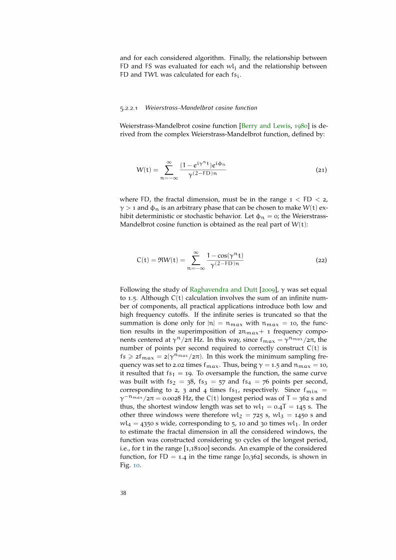
5.2.2.1 Weierstrass-Mandelbrot cosine function
Weierstrass-Mandelbrot cosine function [Berry and Lewis, 1980] is de-rived from the complex Weierstrass-Mandelbrot function, defined by:
W(t) =
∞∑n=−∞
(1− eiγnt)eiφn
γ(2−FD)n(21)
where FD, the fractal dimension, must be in the range 1 < FD < 2,γ > 1 and φn is an arbitrary phase that can be chosen to makeW(t) ex-hibit deterministic or stochastic behavior. Let φn = 0; the Weierstrass-Mandelbrot cosine function is obtained as the real part of W(t):
C(t) = <W(t) =
∞∑n=−∞
1− cos(γnt)γ(2−FD)n
(22)
Following the study of Raghavendra and Dutt [2009], γ was set equalto 1.5. Although C(t) calculation involves the sum of an infinite num-ber of components, all practical applications introduce both low andhigh frequency cutoffs. If the infinite series is truncated so that thesummation is done only for |n| = nmax with nmax = 10, the func-tion results in the superimposition of 2nmax+ 1 frequency compo-nents centered at γn/2π Hz. In this way, since fmax = γnmax/2π, thenumber of points per second required to correctly construct C(t) isfs > 2fmax = 2(γnmax/2π). In this work the minimum sampling fre-quency was set to 2.02 times fmax. Thus, being γ = 1.5 and nmax = 10,it resulted that fs1 = 19. To oversample the function, the same curvewas built with fs2 = 38, fs3 = 57 and fs4 = 76 points per second,corresponding to 2, 3 and 4 times fs1, respectively. Since fmin =
γ−nmax/2π = 0.0028 Hz, the C(t) longest period was of T = 362 s andthus, the shortest window length was set to wl1 = 0.4T = 145 s. Theother three windows were therefore wl2 = 725 s, wl3 = 1450 s andwl4 = 4350 s wide, corresponding to 5, 10 and 30 times wl1. In orderto estimate the fractal dimension in all the considered windows, thefunction was constructed considering 50 cycles of the longest period,i.e., for t in the range [1,18100] seconds. An example of the consideredfunction, for FD = 1.4 in the time range [0,362] seconds, is shown inFig. 10.
38
5.2.2.2 Takagi-Landsberg function
The Takagi-Landsberg function, explored by Takagi [1903], is a curveconstructed by positive mid-point displacements of straight line seg-ments. It is defined on the unit interval by:
T(t) =
∞∑n=0
an∆(bnt) (23)
where a ∈ [0,1], b is an integer greater than 1 and ∆(x), defined by∆(x) = mink∈Z |x− k|, represents the distance from x to the nearestinteger. This function is everywhere continuous but nowhere differ-entiable if ab > 1. In this work, following the study of Raghavendraand Dutt [2009], b = 2 and a ∈ [0.5,1] so that the fractal dimensionFD =
log4alogb could be varied from 1.1 to 1.9 in steps of 0.1. If the infi-
nite summation is approximated by the finite superimposition of thefew first terms and nmax = 10, the function is the result of the sum-mation of nmax+ 1 triangular waves of frequency bn Hz (neglectingharmonic terms). In this way, being fmax about equal to bnmax , thenumber of points required to correctly construct one period of T(t) isfs > 2bnmax . The minimum number of points per second was cho-sen as fs1 = 2.02fmax = 2068. To oversample the function, the samecurve was built with fs2 = 4136, fs3 = 6204 and fs4 = 8272 points persecond. Since fmin = 1 Hz, TWLs were set to wl1 = 0.4 s, wl2 = 2
s, wl3 = 4 s and wl4 = 12 s. In order to estimate FD for all windowlengths, the function was constructed considering 50 periods, i.e., fort in the range [1,50] seconds. An example of the considered function,for FD = 1.4 in the time range [0,1] seconds, is shown in Fig. 10.
5.2.2.3 Fractional Brownian motion
The fBm traces used in this work were generated following the wavelet-based synthesis method proposed by Abry and Sellan [1996]. The orig-inal time-series was built with 128 points per second, the same ratethat will be used to resample EEG traces, in order to produce a spectralcontent limited to about 50 Hz and therefore similar to that of the elec-troencephalogram. The series with sampling frequency fs1 = 128 Hzwas then interpolated to obtain oversampled fs2 = 256 Hz, fs3 = 384
Hz and fs4 = 512 Hz sequences with about the same frequency con-tent. Since fmin = 1 Hz, as observed from the spectra of synthesizedsignals, the shortest TWL was set to wl1 = 0.4
fmin= 0.4 s. The other
three windows were therefore wl2 = 2 s, wl3 = 4 s and wl4 = 12 swide, corresponding to 5, 10 and 30 times wl1. An example of theconsidered function, for FD = 1.4 in the time range [0,1] seconds, isshown in Fig. 10.
5.2.3 EEG analysis
EEGs analyzed in the present study were recorded from 20 healthy Material
39
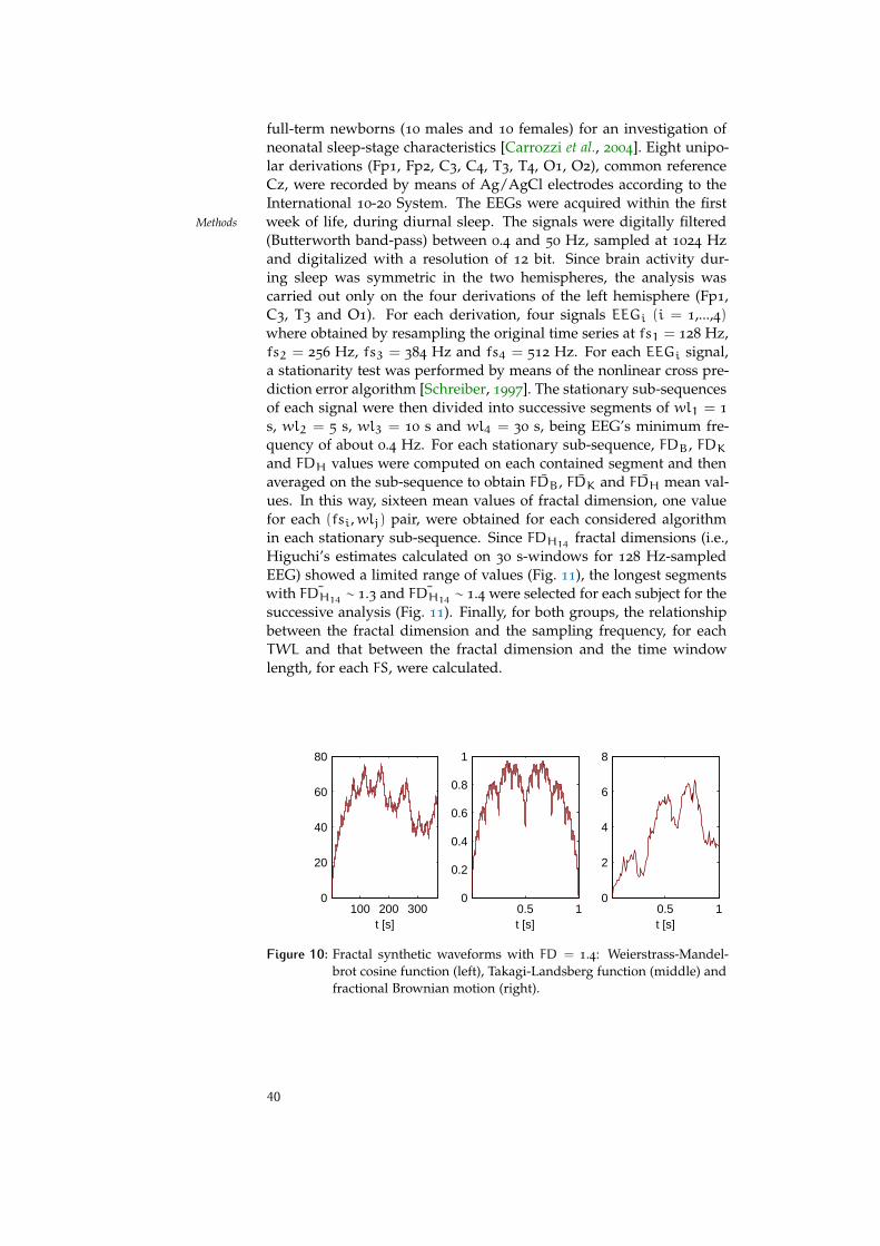
full-term newborns (10 males and 10 females) for an investigation ofneonatal sleep-stage characteristics [Carrozzi et al., 2004]. Eight unipo-lar derivations (Fp1, Fp2, C3, C4, T3, T4, O1, O2), common referenceCz, were recorded by means of Ag/AgCl electrodes according to theInternational 10-20 System. The EEGs were acquired within the firstweek of life, during diurnal sleep. The signals were digitally filteredMethods
(Butterworth band-pass) between 0.4 and 50 Hz, sampled at 1024 Hzand digitalized with a resolution of 12 bit. Since brain activity dur-ing sleep was symmetric in the two hemispheres, the analysis wascarried out only on the four derivations of the left hemisphere (Fp1,C3, T3 and O1). For each derivation, four signals EEGi (i = 1,...,4)where obtained by resampling the original time series at fs1 = 128 Hz,fs2 = 256 Hz, fs3 = 384 Hz and fs4 = 512 Hz. For each EEGi signal,a stationarity test was performed by means of the nonlinear cross pre-diction error algorithm [Schreiber, 1997]. The stationary sub-sequencesof each signal were then divided into successive segments of wl1 = 1
s, wl2 = 5 s, wl3 = 10 s and wl4 = 30 s, being EEG’s minimum fre-quency of about 0.4 Hz. For each stationary sub-sequence, FDB, FDKand FDH values were computed on each contained segment and thenaveraged on the sub-sequence to obtain ¯FDB, ¯FDK and ¯FDH mean val-ues. In this way, sixteen mean values of fractal dimension, one valuefor each (fsi,wlj) pair, were obtained for each considered algorithmin each stationary sub-sequence. Since FDH14 fractal dimensions (i.e.,Higuchi’s estimates calculated on 30 s-windows for 128 Hz-sampledEEG) showed a limited range of values (Fig. 11), the longest segmentswith ¯FDH14 ∼ 1.3 and ¯FDH14 ∼ 1.4 were selected for each subject for thesuccessive analysis (Fig. 11). Finally, for both groups, the relationshipbetween the fractal dimension and the sampling frequency, for eachTWL and that between the fractal dimension and the time windowlength, for each FS, were calculated.
100 200 3000
20
40
60
80
t [s]0.5 1
0
0.2
0.4
0.6
0.8
1
t [s]0.5 1
0
2
4
6
8
t [s]
Figure 10: Fractal synthetic waveforms with FD = 1.4: Weierstrass-Mandel-brot cosine function (left), Takagi-Landsberg function (middle) andfractional Brownian motion (right).
40
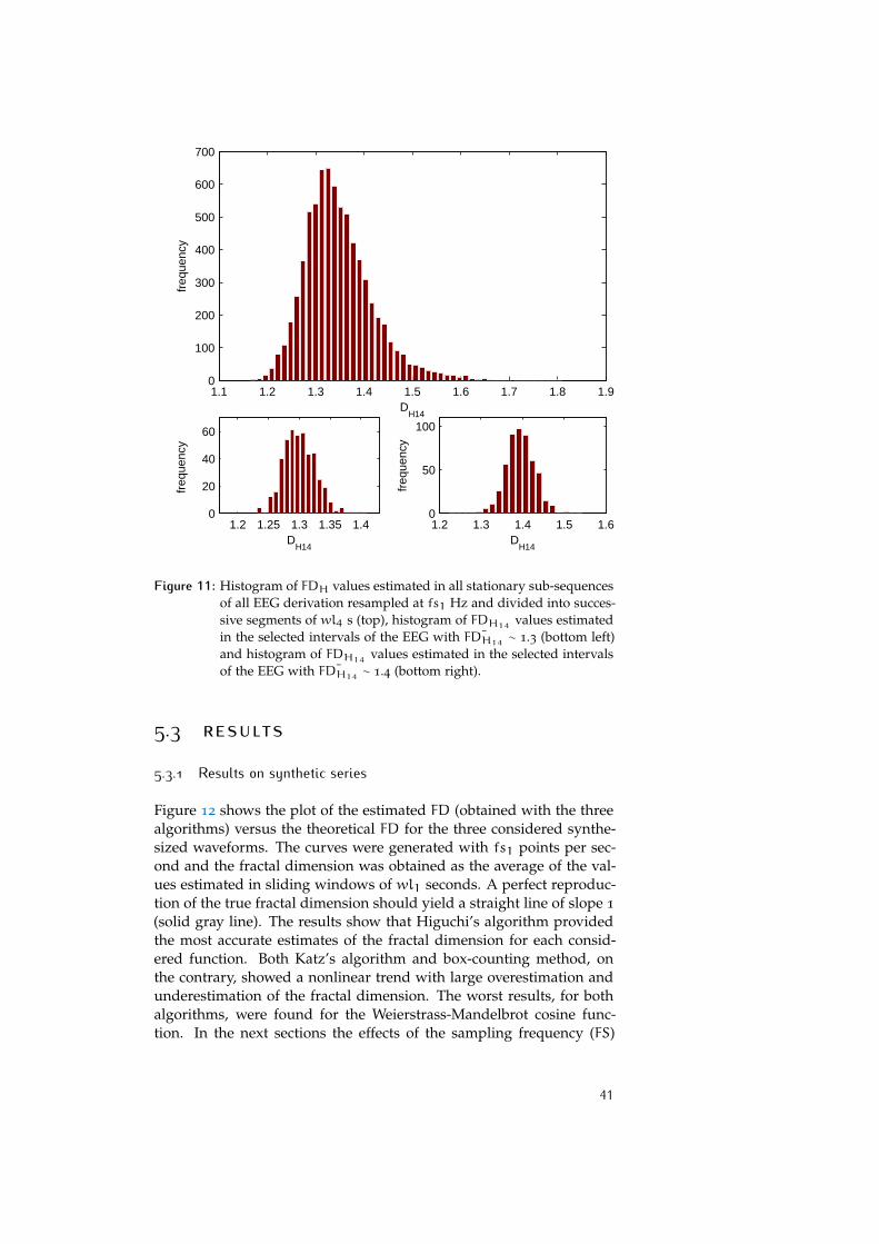
1.1 1.2 1.3 1.4 1.5 1.6 1.7 1.8 1.90
100
200
300
400
500
600
700
DH14
freq
uenc
y
1.2 1.25 1.3 1.35 1.40
20
40
60
DH14
freq
uenc
y
1.2 1.3 1.4 1.5 1.60
50
100
DH14
freq
uenc
y
Figure 11: Histogram of FDH values estimated in all stationary sub-sequencesof all EEG derivation resampled at fs1 Hz and divided into succes-sive segments of wl4 s (top), histogram of FDH14 values estimatedin the selected intervals of the EEG with ¯FDH14 ∼ 1.3 (bottom left)and histogram of FDH14 values estimated in the selected intervalsof the EEG with ¯FDH14 ∼ 1.4 (bottom right).
5.3 results
5.3.1 Results on synthetic series
Figure 12 shows the plot of the estimated FD (obtained with the threealgorithms) versus the theoretical FD for the three considered synthe-sized waveforms. The curves were generated with fs1 points per sec-ond and the fractal dimension was obtained as the average of the val-ues estimated in sliding windows of wl1 seconds. A perfect reproduc-tion of the true fractal dimension should yield a straight line of slope 1
(solid gray line). The results show that Higuchi’s algorithm providedthe most accurate estimates of the fractal dimension for each consid-ered function. Both Katz’s algorithm and box-counting method, onthe contrary, showed a nonlinear trend with large overestimation andunderestimation of the fractal dimension. The worst results, for bothalgorithms, were found for the Weierstrass-Mandelbrot cosine func-tion. In the next sections the effects of the sampling frequency (FS)
41
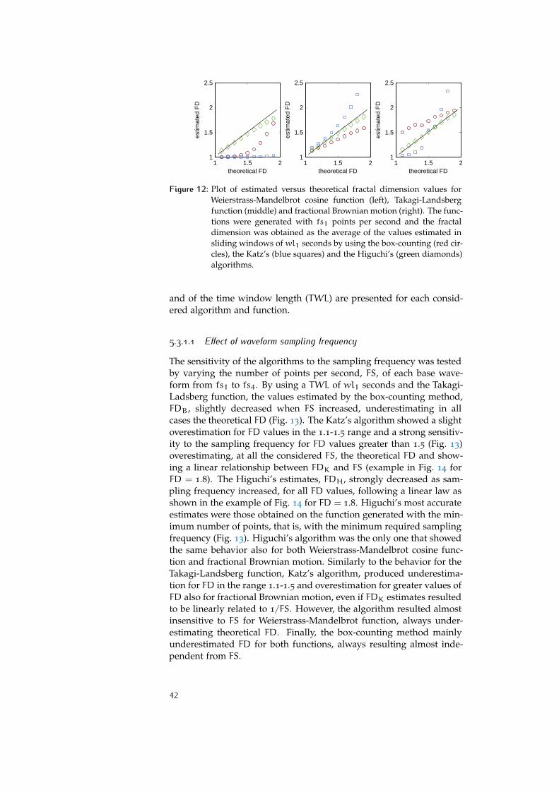
1 1.5 21
1.5
2
2.5
theoretical FD
estim
ated
FD
1 1.5 21
1.5
2
2.5
theoretical FD
estim
ated
FD
1 1.5 21
1.5
2
2.5
theoretical FD
estim
ated
FD
Figure 12: Plot of estimated versus theoretical fractal dimension values forWeierstrass-Mandelbrot cosine function (left), Takagi-Landsbergfunction (middle) and fractional Brownian motion (right). The func-tions were generated with fs1 points per second and the fractaldimension was obtained as the average of the values estimated insliding windows of wl1 seconds by using the box-counting (red cir-cles), the Katz’s (blue squares) and the Higuchi’s (green diamonds)algorithms.
and of the time window length (TWL) are presented for each consid-ered algorithm and function.
5.3.1.1 Effect of waveform sampling frequency
The sensitivity of the algorithms to the sampling frequency was testedby varying the number of points per second, FS, of each base wave-form from fs1 to fs4. By using a TWL of wl1 seconds and the Takagi-Ladsberg function, the values estimated by the box-counting method,FDB, slightly decreased when FS increased, underestimating in allcases the theoretical FD (Fig. 13). The Katz’s algorithm showed a slightoverestimation for FD values in the 1.1-1.5 range and a strong sensitiv-ity to the sampling frequency for FD values greater than 1.5 (Fig. 13)overestimating, at all the considered FS, the theoretical FD and show-ing a linear relationship between FDK and FS (example in Fig. 14 forFD = 1.8). The Higuchi’s estimates, FDH, strongly decreased as sam-pling frequency increased, for all FD values, following a linear law asshown in the example of Fig. 14 for FD = 1.8. Higuchi’s most accurateestimates were those obtained on the function generated with the min-imum number of points, that is, with the minimum required samplingfrequency (Fig. 13). Higuchi’s algorithm was the only one that showedthe same behavior also for both Weierstrass-Mandelbrot cosine func-tion and fractional Brownian motion. Similarly to the behavior for theTakagi-Landsberg function, Katz’s algorithm, produced underestima-tion for FD in the range 1.1-1.5 and overestimation for greater values ofFD also for fractional Brownian motion, even if FDK estimates resultedto be linearly related to 1/FS. However, the algorithm resulted almostinsensitive to FS for Weierstrass-Mandelbrot function, always under-estimating theoretical FD. Finally, the box-counting method mainlyunderestimated FD for both functions, always resulting almost inde-pendent from FS.
42

1 1.5 21
1.5
2
2.5
theoretical FD
FD
B
1 1.5 21
1.5
2
2.5
theoretical FD
FD
K
1 1.5 21
1.5
2
2.5
theoretical FD
FD
H
Figure 13: Plot of estimated versus theoretical fractal dimension for the Takagi-Landsberg function, for different values of FS, obtained with box-counting method (left), Katz’s algorithm (middle) and Higuchi’salgorithm (right) on estimation windows of wl1 seconds. fs1: redcircles, fs2: blue squares, fs3: green diamonds, fs4: black penta-grams.
fs1 fs2 fs3 fs41.4
1.45
1.5
1.55
FD
B
fs1 fs2 fs3 fs41.6
1.8
2
2.2
2.4
FD
K
fs1 fs2 fs3 fs41.3
1.5
1.7
1.9
FD
H
Figure 14: Plot of estimated fractal dimension versus FS, for different valuesof TWL, for the Takagi-Landsberg function of FD = 1.8, obtainedwith box-counting method (left), Katz’s algorithm (middle) andHiguchi’s algorithm (right). wl1: red circles, wl2: blue squares,wl3: green diamonds, wl4: black pentagrams.
5.3.1.2 Effect of estimation time window length
The dependence on the time window length was studied by varyingTWL from wl1 to wl4 seconds considering a FS value of fs1. The box-counting method turned out to be sensitive to the time window lengthonly for fBm function, with FDB slightly decreasing with TWL, whileit underestimated the theoretical FD for the other two functions in-dependently from TWL (examples for the Takagi-Landsberg functionin Figs. 15 and 16). On the contrary, a clear dependence on the TWLwas exhibited by Katz’s algorithm for both fractional Brownian motionand Takagi-Landsberg function (examples in Figs. 15 and 16) produc-ing underestimation and overestimation of theoretical FD, respectively.In both cases the FDK estimates decreased as TWL increased follow-ing a nonlinear law. For the Weierstrass-Mandelbrot cosine functionFDK values were very close to 1 for all the considered TWL. Finally,Higuchi’s algorithm turned out to be independent from the TWL forall the considered functions (examples in Figs. 15 and 16).
43

1 1.5 21
1.5
2
2.5
theoretical FD
FD
B
1 1.5 21
1.5
2
2.5
theoretical FD
FD
K
1 1.5 21
1.5
2
2.5
theoretical FD
FD
H
Figure 15: Plot of estimated versus theoretical fractal dimension for the Takagi-Landsberg function, built with fs1 points per second, for differentvalues of TWL, obtained with box-counting method (left), Katz’s al-gorithm (middle) and Higuchi’s algorithm (right). wl1: red circles,wl2: blue squares, wl3: green diamonds, wl4: black pentagrams.
wl1wl2wl3 wl41.4
1.45
1.5
1.55
FD
B
wl1wl2wl3 wl41.6
1.8
2
2.2
2.4
FD
K
wl1wl2wl3 wl41.3
1.5
1.7
1.9
FD
H
Figure 16: Plot of estimated fractal dimension versus TWL, for different val-ues of FS, for the Takagi-Landsberg function of FD = 1.8, obtainedwith box-counting method (left), Katz’s algorithm (middle) andHiguchi’s algorithm (right). fs1: red circles, fs2: blue squares, fs3:green diamonds, fs4: black pentagrams.
5.3.2 Results on the EEG
Based on the results on the synthetic series, the performances of thethree considered algorithms were evaluated on EEG traces in terms ofsensitivity to both the FS and the TWL, considering the estimates ofthe Higuchi’s algorithm as the most reliable ones.
5.3.2.1 Effect of EEG sampling frequency
Figure 17 (left column) shows that the box-counting estimate, FDB, cal-culated on the segments in which the Higuchi’s estimate ¯FDH14 was ofabout 1.3 (or 1.4), decreased as FS increased in a different way for eachwlj value. On the other hand, both Katz’s and Higuchi’s estimateslinearly decreased with 1/fs according to the following relationship:
FDj =mj
fs+ qj (24)
for j = 1,...,4. The values of the mj and qj coefficients, obtained byusing Katz’s ( ¯mKj, ¯qKj) and Higuchi’s ( ¯mHj, ¯qHj) algorithms by aver-aging on the subjects, for fractal values ( ¯FDH14 ) of about 1.3 and 1.4,are listed in Tab. 3 and in Tab. 4, respectively.
44
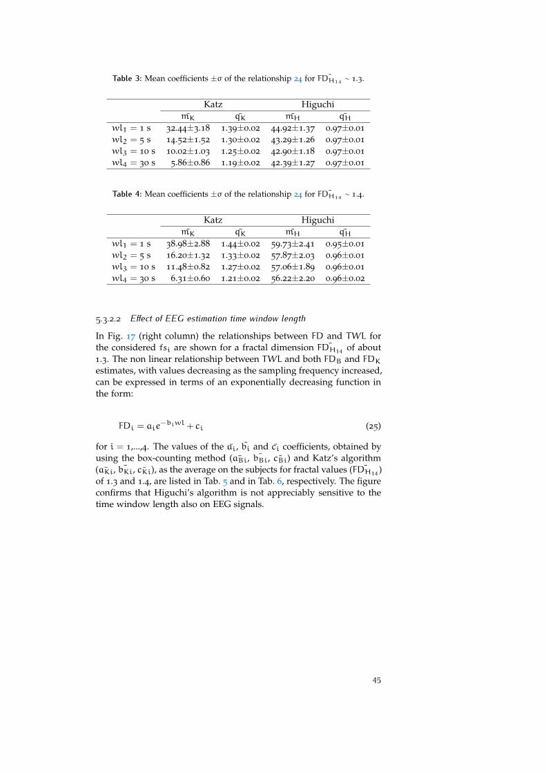
Table 3: Mean coefficients ±σ of the relationship 24 for ¯FDH14 ∼ 1.3.
Katz HiguchimK qK mH ¯qH
wl1 = 1 s 32.44±3.18 1.39±0.02 44.92±1.37 0.97±0.01
wl2 = 5 s 14.52±1.52 1.30±0.02 43.29±1.26 0.97±0.01
wl3 = 10 s 10.02±1.03 1.25±0.02 42.90±1.18 0.97±0.01
wl4 = 30 s 5.86±0.86 1.19±0.02 42.39±1.27 0.97±0.01
Table 4: Mean coefficients ±σ of the relationship 24 for ¯FDH14 ∼ 1.4.
Katz HiguchimK qK mH ¯qH
wl1 = 1 s 38.98±2.88 1.44±0.02 59.73±2.41 0.95±0.01
wl2 = 5 s 16.20±1.32 1.33±0.02 57.87±2.03 0.96±0.01
wl3 = 10 s 11.48±0.82 1.27±0.02 57.06±1.89 0.96±0.01
wl4 = 30 s 6.31±0.60 1.21±0.02 56.22±2.20 0.96±0.02
5.3.2.2 Effect of EEG estimation time window length
In Fig. 17 (right column) the relationships between FD and TWL forthe considered fsi are shown for a fractal dimension ¯FDH14 of about1.3. The non linear relationship between TWL and both FDB and FDKestimates, with values decreasing as the sampling frequency increased,can be expressed in terms of an exponentially decreasing function inthe form:
FDi = aie−biwl + ci (25)
for i = 1,...,4. The values of the ai, bi and ci coefficients, obtained byusing the box-counting method ( ¯aBi, ¯bBi, ¯cBi) and Katz’s algorithm( ¯aKi, ¯bKi, ¯cKi), as the average on the subjects for fractal values ( ¯FDH14 )of 1.3 and 1.4, are listed in Tab. 5 and in Tab. 6, respectively. The figureconfirms that Higuchi’s algorithm is not appreciably sensitive to thetime window length also on EEG signals.
45
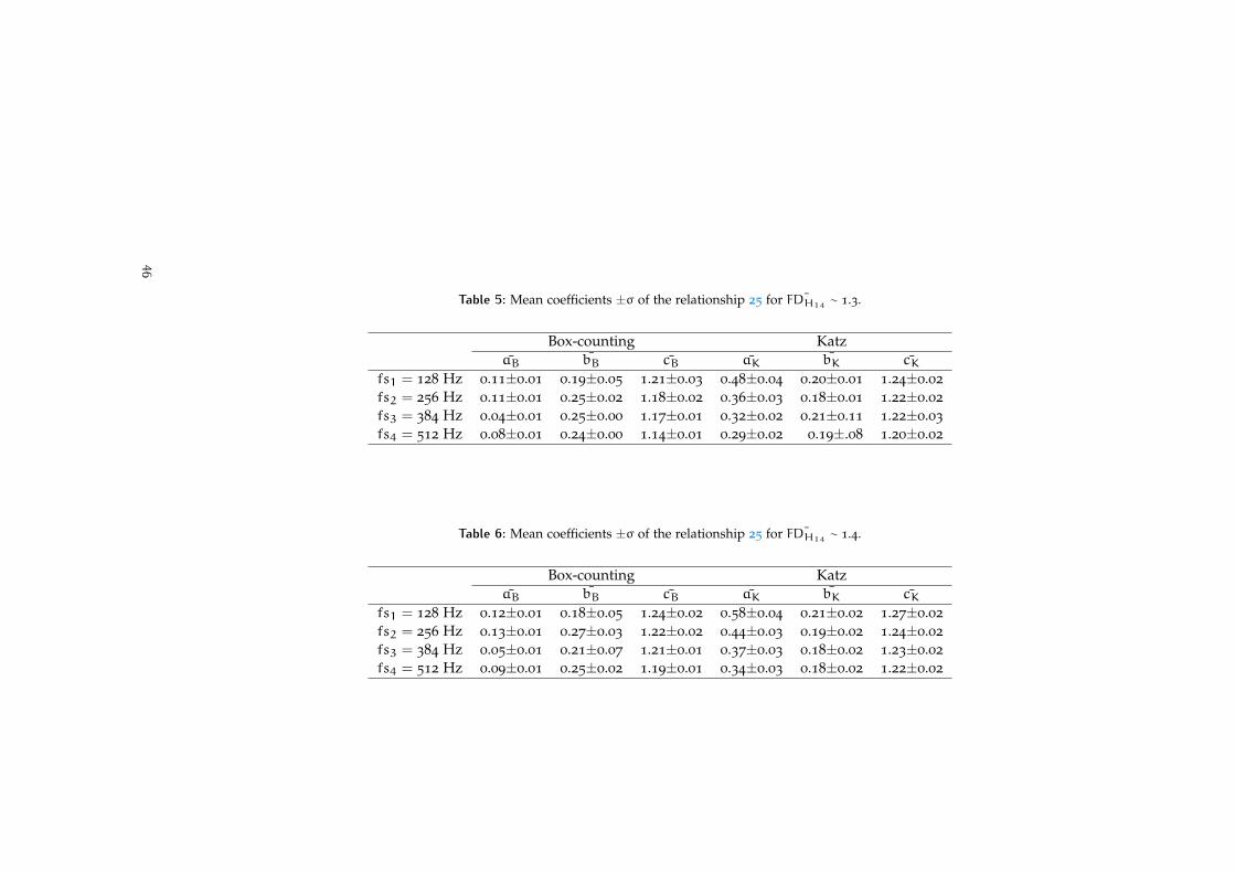
Table 5: Mean coefficients ±σ of the relationship 25 for ¯FDH14 ∼ 1.3.
Box-counting KatzaB bB cB aK bK cK
fs1 = 128 Hz 0.11±0.01 0.19±0.05 1.21±0.03 0.48±0.04 0.20±0.01 1.24±0.02
fs2 = 256 Hz 0.11±0.01 0.25±0.02 1.18±0.02 0.36±0.03 0.18±0.01 1.22±0.02
fs3 = 384 Hz 0.04±0.01 0.25±0.00 1.17±0.01 0.32±0.02 0.21±0.11 1.22±0.03
fs4 = 512 Hz 0.08±0.01 0.24±0.00 1.14±0.01 0.29±0.02 0.19±.08 1.20±0.02
Table 6: Mean coefficients ±σ of the relationship 25 for ¯FDH14 ∼ 1.4.
Box-counting KatzaB bB cB aK bK cK
fs1 = 128 Hz 0.12±0.01 0.18±0.05 1.24±0.02 0.58±0.04 0.21±0.02 1.27±0.02
fs2 = 256 Hz 0.13±0.01 0.27±0.03 1.22±0.02 0.44±0.03 0.19±0.02 1.24±0.02
fs3 = 384 Hz 0.05±0.01 0.21±0.07 1.21±0.01 0.37±0.03 0.18±0.02 1.23±0.02
fs4 = 512 Hz 0.09±0.01 0.25±0.02 1.19±0.01 0.34±0.03 0.18±0.02 1.22±0.02
46
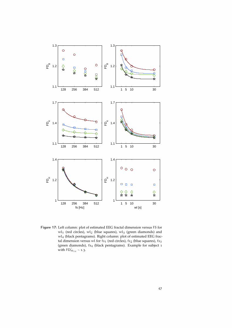
128 256 384 5121.1
1.2
1.3F
DB
128 256 384 5121.1
1.4
1.7
FD
K
128 256 384 5121
1.2
1.4
fs [Hz]
FD
H
1 5 10 301.1
1.2
1.3
FD
B
1 5 10 301.1
1.4
1.7F
DK
1 5 10 301
1.2
1.4
wl [s]
FD
H
Figure 17: Left column: plot of estimated EEG fractal dimension versus FS forwl1 (red circles), wl2 (blue squares), wl3 (green diamonds) andwl4 (black pentagrams). Right column: plot of estimated EEG frac-tal dimension versus wl for fs1 (red circles), fs2 (blue squares), fs3(green diamonds), fs4 (black pentagrams). Example for subject 1
with ¯FDH14 ∼ 1.3.
47
5.4 discussion
The test on the synthetic functions of known fractal dimension, per-formed at the appropriate sampling frequency observing Nyquist-Shan-non sampling theorem without oversampling, partially confirmed theresults of previous studies [Accardo et al., 1997; Esteller et al., 2001;Paramanathan and Uthayakumar, 2008; Raghavendra and Dutt, 2009],i.e., Higuchi’s algorithm provides the most accurate estimates of thefractal dimension. However, some conflicting results have been ob-tained when analyzing the dependence of FD estimates on the two con-sidered factors: the sampling frequency and the time window length.
Contrary to the results of Raghavendra and Dutt [2009], in whichSensitivity to FS
Higuchi’s algorithm estimation accuracy improved as the samplingfrequency increased, with FDH values slightly affected by the sam-pling frequency, the reported results showed that Higuchi’s method isstrongly dependent on the sampling frequency and FDH estimates im-proved as the sampling frequency decreased toward the Nyquist rate,i.e., to the lower bound for aliasing-free signal sampling. On the otherhand, in agreement with the aforementioned study, Katz’s algorithmturned out to be dependent on the sampling frequency, providing esti-mates that decreased with the sampling frequency.
With regard to the sensitivity to the time window length, the studySensitivity to TWL
of Esteller et al. [2001] showed that the fractal dimension estimatesobtained with Higuchi’s algorithm improved as the window lengthincreased, while the study of Paramanathan and Uthayakumar [2008]did not report any dependence on TWL. The analysis performed inthe present study indicated that Higuchi’s estimates are correct inde-pendently from the time window length, provided that a suitable sam-pling frequency is used. Both the aforementioned studies highlighteda slight sensitivity to TWL of Katz’s algorithm while the present studyshowed a strong dependence on the time window length.
The fractal analysis of the EEG basically confirmed the results of theinvestigation carried out on the synthetic functions. The box-countingmethod turned out to be sensitive to both the sampling frequency andthe time window length, although a clear relationship could be ex-pressed only between FDB and TWL. Moreover, the results supportedthe dependence of Katz’s estimates on both factors and confirmed thatHiguchi’s algorithm is sensitive only to the sampling frequency.
Thus, although the fractal dimension of the EEG signals is not knowna priori, based on the results on synthetic signals it can be asserted thatthe most correct estimates were those provided by Higuchi’s algorithmat the lowest considered sampling frequency (128 Hz). This value, ob-serving the Nyquist-Shannon sampling theorem, is about 2.5 times theLP cut-off frequency, which was chosen according to the frequencycontent of the EEG recorded from sleeping newborns, which is limitedto about 40 Hz. Hence, in order to conduct an accurate fractal anal-ysis, it is of primary importance to adapt the sampling frequency tothe bandwidth of the considered EEG and, therefore, to the selectedlow-pass cutoff frequency. A sampling frequency close to 2.5 times
48
the cutoff frequency of a third order low-pass filter could represent anoptimal choice to avoid underestimation of the fractal dimension dueto oversampling. This solution also prevents the reduction of the dy-namic range of the fractal dimension. Higuchi’s algorithm, being notsensitive to the time window length, it is also preferable for real-timeapplications in which short epochs have to be examined.
It is nonetheless true that in some investigations it might be not inter-esting the true value of the fractal dimension, but rather its fluctuationover time or the differences among the values estimated in differentconditions. In this cases, methods different from Higuchi’s algorithmcould be also used for the fractal analysis. In any case, whenever twoor more studies have to be compared, it is necessary to take into ac-count the sampling frequency and the time window length used ineach investigation.
5.5 conclusionIn this study the performances of three algorithms commonly used forthe estimation of EEG fractal dimension were compared in terms ofaccuracy and sensitivity to the sampling frequency and to the timewindow length. The investigation was carried out firstly on threesynthetic functions of known fractal dimension and then on 20 EEGsrecorded from as many sleeping newborns. Results indicate that thebox-counting algorithm is the least reliable method, providing incor-rect estimates also dependent on both the sampling frequency and theestimation window length. The Katz’s algorithm, though sensitive toboth factors, turned out to be more reliable and produced some accu-rate estimates. However, the study suggests that Higuchi’s algorithmis the most accurate of the considered methods, provided that the sig-nals are not oversampled. Furthermore, it is appropriate to estimatethe fractal dimension of events of both brief duration as well as longerEEG traces, being the estimates not dependent on the time windowlength. In any case, information about the sampling frequency andthe time window length should always accompany the results of thefractal analysis, since it is relevant for its correct interpretation.
49

6 E E G V S F B M S C A L I N G L A W
contents6.1 Introduction and motivation 516.2 Materials and Methods 526.3 Results 536.4 Discussion 556.5 Conclusion 57
This chapter presents an investigation carried out to verify the ac-curacy of fractional Brownian motion to model the EEG. The studyis inspired by the widespread practice of using fBm theoretical re-lationships of Eq. 14 to equivalently characterize the scaling proper-ties of the EEG. The fractal dimension (FD) and the power-law ex-ponent (β) are independently estimated on 536 EEG traces acquiredfrom healthy full-term sleeping newborns, children, young adults andelderly adults. Experimental relationships between FD and β are calcu-lated and compared among the populations to detect possible scalingdifferences related to age. Mean experimental relationships are thencalculated within each group and compared with the scaling relation-ship of Eq. 14 in order to detect possible deviations from fBm. Thechapter is partially based on Author’s publication 3.
6.1 introduction and motivation
The scaling behavior of self-affine time series can be equivalently char-acterized by the fractal dimension (FD), the power-law exponent (β)and the Hurst index (H). Whereas the fractal dimension and the Hurstindex are related by the simple equation, FD = 2 −H, the relation-ship existing between FD and β is unsettled [Higuchi, 1990]. Consider,for example, the Weierstrass function, XH(t) [Bassingthwaighte et al.,1994], of Fig. 8. As described in Chapter 4.5, this function consists ofan infinite summation of periodic terms, each of which has a frequencythat is a factor b larger than the preceding term and an amplitude thatis a times smaller. Whereas self-similarity represents the property ofthe shapes to be identical under magnification, self-affinity expressesthe necessity to scale down XH and t by different amounts (∆XH and∆t, respectively) to obtain two identical views. In particular, if a,b > 1
and bH = a then ∆XH = ∆tH, whit H ranging from 0 to 1. The re-lationship between the fractal dimension and the power-law exponent
51
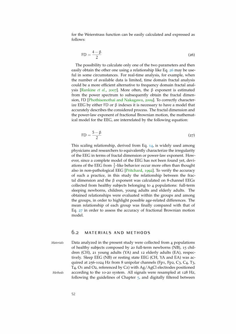
for the Weierstrass function can be easily calculated and expressed asfollows:
FD =4−β
2(26)
The possibility to calculate only one of the two parameters and theneasily obtain the other one using a relationship like Eq. 26 may be use-ful in some circumstances. For real-time analysis, for example, whenthe number of available data is limited, time domain fractal analysiscould be a more efficient alternative to frequency domain fractal anal-ysis [Rankine et al., 2007]. More often, the β exponent is estimatedfrom the power spectrum to subsequently obtain the fractal dimen-sion, FD [Phothisonothai and Nakagawa, 2009]. To correctly character-ize EEG by either FD or β indexes it is necessary to have a model thataccurately describes the considered process. The fractal dimension andthe power-law exponent of fractional Brownian motion, the mathemat-ical model for the EEG, are interrelated by the following equation:
FD =5−β
2(27)
This scaling relationship, derived from Eq. 14, is widely used amongphysicians and researchers to equivalently characterize the irregularityof the EEG in terms of fractal dimension or power-law exponent. How-ever, since a complete model of the EEG has not been found yet, devi-ations of the EEG from 1
f -like behavior occur more often than thoughtalso in non-pathological EEG [Pritchard, 1992]. To verify the accuracyof such a practice, in this study the relationship between the frac-tal dimension and the β exponent was calculated on 8-channel EEGscollected from healthy subjects belonging to 4 populations: full-termsleeping newborns, children, young adults and elderly adults. Theobtained relationships were evaluated within the groups and amongthe groups, in order to highlight possible age-related differences. Themean relationship of each group was finally compared with that ofEq. 27 in order to assess the accuracy of fractional Brownian motionmodel.
6.2 materials and methodsData analyzed in the present study were collected from 4 populationsMaterials
of healthy subjects composed by 20 full-term newborns (NB), 15 chil-dren (CH), 21 young adults (YA) and 12 elderly adults (EA), respec-tively. Sleep EEG (NB) or resting state EEG (CH, YA and EA) was ac-quired at 256-1024 Hz from 8 unipolar channels (Fp1, Fp2, C3, C4, T3,T4, O1 and O2, referenced by Cz) with Ag/AgCl electrodes positionedaccording to the 10-20 system. All signals were resampled at 128 Hz,Methods
following the guidelines of Chapter 5, and digitally filtered between
52
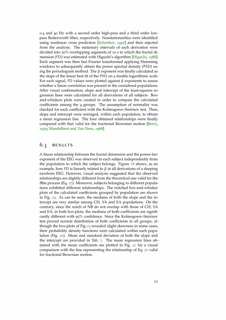
0.4 and 40 Hz with a second order high-pass and a third order low-pass Butterworth filter, respectively. Nonstationarities were identifiedusing nonlinear cross prediction [Schreiber, 1997] and then rejectedfrom the analysis. The stationary intervals of each derivation weredivided into 50% overlapping segments of 10 s in which the fractal di-mension (FD) was estimated with Higuchi’s algorithm [Higuchi, 1988].Each segment was then fast Fourier transformed applying Hammingwindows to subsequently obtain the power spectral density (PSD) us-ing the periodogram method. The β exponent was finally calculated asthe slope of the linear best fit of the PSD on a double logarithmic scale.For each signal, FD values were plotted against β exponents to assesswhether a linear correlation was present in the considered populations.After visual confirmation, slope and intercept of the least-squares re-gression lines were calculated for all derivations of all subjects. Box-and-whiskers plots were created in order to compare the calculatedcoefficients among the 4 groups. The assumption of normality waschecked for each coefficient with the Kolmogorov-Smirnov test. Then,slope and intercept were averaged, within each population, to obtaina mean regression line. The four obtained relationships were finallycompared with that valid for the fractional Brownian motion [Berry,1979; Mandelbrot and Van Ness, 1968].
6.3 resultsA linear relationship between the fractal dimension and the power-lawexponent of the EEG was observed in each subject independently fromthe population to which the subject belongs. Figure 18 shows, as anexample, how FD is linearly related to β in all derivations of a sleepingnewborn EEG. However, visual analysis suggested that the observedrelationships are slightly different from the theoretical one valid for thefBm process (Eq. 27). Moreover, subjects belonging to different popula-tions exhibited different relationships. The notched box-and-whiskerplots of the calculated coefficients grouped by population are shownin Fig. 19. As can be seen, the medians of both the slope and the in-tercept are very similar among CH, YA and EA populations. On thecontrary, since the notch of NB do not overlap with those of CH, YAand EA, in both box-plots, the medians of both coefficients are signifi-cantly different with 95% confidence. Since the Kolmogorov-Smirnovtest proved normal distribution of both coefficients in all groups, al-though the box-plots of Fig 19 revealed slight skewness in some cases,their probability density functions were calculated within each popu-lation (Fig. 20). Mean and standard deviation of both the slope andthe intercept are provided in Tab. 7. The mean regression lines ob-tained with the mean coefficients are plotted in Fig. 21 for a visualcomparison with the line representing the relationship of Eq. 27 validfor fractional Brownian motion.
53
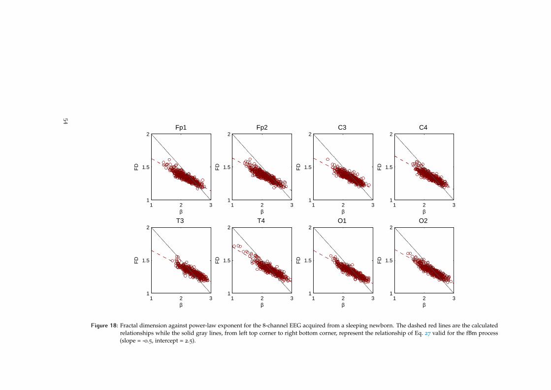
1 2 31
1.5
2Fp1
β
FD
1 2 31
1.5
2Fp2
βF
D
1 2 31
1.5
2C3
β
FD
1 2 31
1.5
2C4
β
FD
1 2 31
1.5
2T3
β
FD
1 2 31
1.5
2T4
β
FD
1 2 31
1.5
2O1
βF
D1 2 3
1
1.5
2O2
β
FD
Figure 18: Fractal dimension against power-law exponent for the 8-channel EEG acquired from a sleeping newborn. The dashed red lines are the calculatedrelationships while the solid gray lines, from left top corner to right bottom corner, represent the relationship of Eq. 27 valid for the fBm process(slope = -0.5, intercept = 2.5).
54
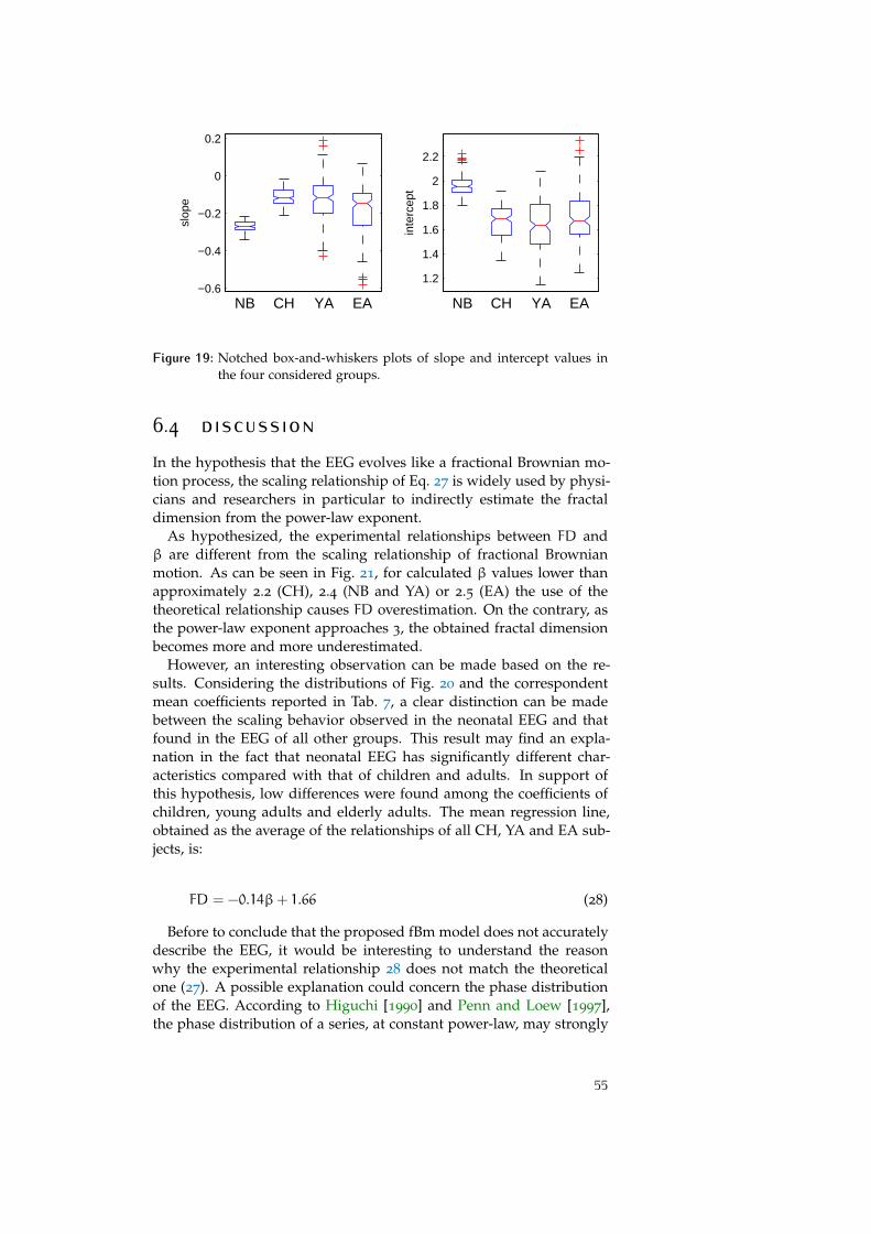
−0.6
−0.4
−0.2
0
0.2
NB CH YA EA
slop
e
1.2
1.4
1.6
1.8
2
2.2
NB CH YA EA
inte
rcep
t
Figure 19: Notched box-and-whiskers plots of slope and intercept values inthe four considered groups.
6.4 discussionIn the hypothesis that the EEG evolves like a fractional Brownian mo-tion process, the scaling relationship of Eq. 27 is widely used by physi-cians and researchers in particular to indirectly estimate the fractaldimension from the power-law exponent.
As hypothesized, the experimental relationships between FD andβ are different from the scaling relationship of fractional Brownianmotion. As can be seen in Fig. 21, for calculated β values lower thanapproximately 2.2 (CH), 2.4 (NB and YA) or 2.5 (EA) the use of thetheoretical relationship causes FD overestimation. On the contrary, asthe power-law exponent approaches 3, the obtained fractal dimensionbecomes more and more underestimated.
However, an interesting observation can be made based on the re-sults. Considering the distributions of Fig. 20 and the correspondentmean coefficients reported in Tab. 7, a clear distinction can be madebetween the scaling behavior observed in the neonatal EEG and thatfound in the EEG of all other groups. This result may find an expla-nation in the fact that neonatal EEG has significantly different char-acteristics compared with that of children and adults. In support ofthis hypothesis, low differences were found among the coefficients ofchildren, young adults and elderly adults. The mean regression line,obtained as the average of the relationships of all CH, YA and EA sub-jects, is:
FD = −0.14β+ 1.66 (28)
Before to conclude that the proposed fBm model does not accuratelydescribe the EEG, it would be interesting to understand the reasonwhy the experimental relationship 28 does not match the theoreticalone (27). A possible explanation could concern the phase distributionof the EEG. According to Higuchi [1990] and Penn and Loew [1997],the phase distribution of a series, at constant power-law, may strongly
55
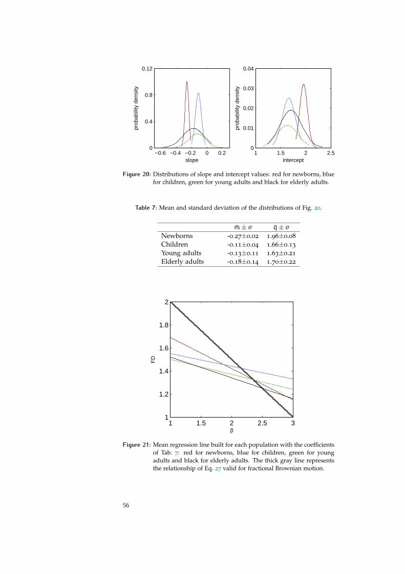
−0.6 −0.4 −0.2 0 0.20
0.4
0.8
0.12
slope
prob
abili
ty d
ensi
ty
1 1.5 2 2.50
0.01
0.02
0.03
0.04
intercept
prob
abili
ty d
ensi
ty
Figure 20: Distributions of slope and intercept values: red for newborns, bluefor children, green for young adults and black for elderly adults.
Table 7: Mean and standard deviation of the distributions of Fig. 20.
m± σ q± σNewborns -0.27±0.02 1.96±0.08
Children -0.11±0.04 1.66±0.13
Young adults -0.13±0.11 1.63±0.21
Elderly adults -0.18±0.14 1.70±0.22
1 1.5 2 2.5 31
1.2
1.4
1.6
1.8
2
β
FD
Figure 21: Mean regression line built for each population with the coefficientsof Tab. 7: red for newborns, blue for children, green for youngadults and black for elderly adults. The thick gray line representsthe relationship of Eq. 27 valid for fractional Brownian motion.
56
affect its behavior in the time domain, producing very different valuesof fractal dimension. Future investigation should attempt to explorethe possible influence of EEG phase distribution on the scaling rela-tionship between FD and β.
6.5 conclusionThe self-affinity of the EEG can be characterized equivalently by eitherfractal dimension or power-law beta exponent. Fractional Brownianmotion, applied to the modeling of the EEG, provides a useful rela-tionship between FD and β, which is currently exploited by many re-searchers and physicians. The results of the study presented in thischapter highlight the inaccuracy of the adopted model which intro-duces errors in the quantitative description of the scaling propertiesof the EEG. Every time absolute values of FD are required for analysispurposes, direct estimation provides more correct values than those in-directly obtained by applying the fBm relationship 27 with lower com-putational effort. Further investigations are necessary to assess howwould the experimental relationships presented in this work change,for example, with pathology or according to the mental task. Based onthe preliminary results reported in this chapter, there is little chancethat a single scaling relationship could be found for the description ofthe fractal-like behavior of the EEG.
57

Part II
Clinical applications
59

7 M O N I TO R I N G C A R OT I DE N DA R T E R E C TO M Y
contents7.1 Introduction and motivation 617.2 Materials and Methods 62
7.2.1 Patients 62
7.2.2 EEG recording and analysis 63
7.2.3 Patients classification 65
7.3 Results 657.4 Discussion 707.5 Conclusion 73
EEG monitoring during carotid endarterectomy is the commonestmethod used to reduce the risk of intraoperative brain ischemia. Be-side visual assessment of the EEG, some quantitative parameters, basedon spectral information, have been recently suggested as additionalcriteria for shunt need decision. This chapter explores new linear(HLF ratio) and nonlinear parameters (ZC and FD) which can assistthe physician in real-time decision whether a shunt is required or not.The results obtained with the proposed parameters are compared withthose achieved by means of three previously explored measures: thedesynchronization index, the sBSI and the tBSI. This chapter is basedon Author’s publication 1.
7.1 introduction and motivationCarotid endarterectomy (CEA) is a well-known surgical procedure for Carotid
endarterectomythe prevention of stroke in patient with high-grade carotid stenosisand is generally performed with selective shunting [Kalkman, 2004].Intraoperative ischemia during carotid cross-clamping in patients un- Intraoperative
ischemiadergoing CEA is a major complication and prompt recognition of insuf-ficient collateral blood supply is crucial (occlusion of the controlateralinternal carotid artery is considered to have a significant impact on theoutcome of CEA).
Different methods have been used to prevent intraoperative stroke: State of the art
the measurement of carotid back pressure [Moore et al., 1973], the as-sessment of the awake patient under regional anaesthesia [Shah et al.,1994], the transcranial Doppler measurement [Ghali et al., 1997], themonitoring of somatosensory evoked potentials [Schweiger et al., 1991],and the continuous EEG monitoring [McFarland et al., 1988; Pinkerton,2002; Plestis et al., 1997; Salvian et al., 2012; Visser et al., 1999]. The lat-ter is still the most used form of monitoring cerebral hypoperfusion
61
during CEA. As EEG visual analysis is subject to human error andmakes quantification of signal’s alterations difficult, it is evident that aquantitative measure should identify more reliably those patients whoneed a shunt during carotid clamping. To this aim, several parametersbased on EEG spectral analysis, producing reasonable results, havebeen recently proposed for the monitoring of CEA [Cursi et al., 2005;van Putten, 2006; van Putten et al., 2004]. They are supported by thefact that a decrease in relative alpha and beta band powers as well aspossible hemispheric asymmetry represent clear signs that the brain isat risk during CEA [Minicucci et al., 2000; Visser et al., 2001]. In order tosupport the physician in a prompt decision whether or not shunting isneeded, the possibility of reliable real-time evaluation and the ease ofinterpretation represent specific characteristics that quantitative EEGmeasures should have.
Based on these requirements, in this chapter some linear and non-Adopted approach
linear EEG parameters that could be useful to monitor the cerebralresponse to significant blood flow reduction are investigated and com-pared with those proposed in the literature [Cursi et al., 2005; van Put-ten, 2006; van Putten et al., 2004]. The new linear parameter (HLF ratio)Proposed parameters
is based on the observation that in presence of brain suffering the spec-tral power decrease in the 8-15 Hz band is very often associated to apower increase in the low frequency band. In order to take into ac-count both behaviors, the ratio between the signal power in the 8-15
Hz and in the 0.5-5 Hz will be considered. The nonlinear parametersthat will be examined are Higuchi’s fractal dimension (FD) and thezero-crossings (ZC), an index for the description of nonlinear systemswhich is dependent on the dominant frequency (or band) of the signal.
7.2 materials and methods
7.2.1 Patients
A total of 140 patients who underwent carotid endarterectomy at theAOTS Hospital of Trieste in 2003-2006 were retrospectively examined.Since artifacts, well recognized by the human observer, are not triviallyeliminated or compensated for by computer programs, the 5 cases inwhich the EEG was so corrupted to make unreliable also the expertassessment were rejected from the study. The remaining 46 femaleand 89 male patients (age of 70±8 years) were considered for the in-vestigation. All CEAs were performed under general anesthesia anddecision to shunt was based on intraoperative EEG monitoring. Selec-tive shunt was advised (21 patients) if the visual inspection of EEG,as interpreted by an experienced neurophysiologist during clampingprocedure, showed significant mono- or bilateral EEG changes. Thesealterations included a decrease in fast activity and/or an increase inslow activity (slowing down in running EEG), or an attenuation of thewhole EEG activity (voltage reduction). The accurate EEG off-line re-analysis finally permitted to reclassify two patients who belonged to
62
the non-shunted group as to be shunted. Hence, on the whole, 112
non-shunted and 23 shunted patients were considered for the classifi-cation.
7.2.2 EEG recording and analysis
EEGs were recorded according to the international 10-20 system with Recording
Ag/AgCl electrodes. The acquisition was performed using GalileoSystem (EBNeuro, Florence, Italy) with a 128 or 512 Hz sampling fre-quency. Ten bipolar derivations were used for the analysis (F4-C4,C4-P4, P4-O2, F8-T6, T6-O2, F3-C3, C3-P3, P3-O1, F7-T5, T5-O1). Al-though some EEG derivations may be more sensitive to anomalies dur-ing carotid endarterectomy than others [Laman et al., 2012], in thiswork all EEG derivations were equally weighted in order to simplifythe procedure. The off-line investigation was carried out during the3 min before and 3 min after the artery clamping, separately for rightand left hemisphere derivations. The signal coming from each deriva- Pre-processing
tion was resampled (if necessary) at 128 Hz, according to the guide-lines of Chapter 5 for the estimation of the fractal dimension, digitallyprocessed with a Butterworth band-pass filter between 0.4 and 40 Hzand divided into 50% overlapping segments of 20 s (2560 points), eachof which was detrended and Hamming windowed. All parameters Parameters
calculationwere calculated in these epochs and averaged among all the deriva-tions of the same hemisphere, obtaining one value per parameter andhemisphere every 10 seconds. The baseline for all parameters wasevaluated from the first 3 min preceding the clamping procedure (ref-erence period), using the median value in this period. Finally, pos-sible variations of the parameters after clamping with respect to thebaseline value were quantified by calculating for each parameter andhemisphere, at each step t, two different functions: the percent relativevariation, R(t), and the Z -score, Z(t), defined as:
R(t) =P(t) − P
P· 100 (29)
and
Z(t) =P(t) − P
σ(30)
where P(t) represents the generic parameter value at step t; P and σcorrespond to the median and the standard deviation values, respec-tively, of the parameter P calculated in the reference period. The R(t)function determines the percent parameter change during clampingcompared to the reference period, while the Z(t) function measuresthe significance of the difference between post-clamping and referenceperiod values. Linear analysis considered some spectral parameters
63
calculated from the power spectral density (PSD) estimated using pe-riodogram method:
PSD =1
N|DFT |2 (31)
DFT being the Discrete Fourier Transform of the EEG. From PSD, theSpectral parameters
power in the traditional EEG sub-bands (delta 0.5-4 Hz, theta 4-8 Hz,alpha 8-13 Hz and beta 13-18 Hz) and the power in a low frequencyband (LF: 0.5-5 Hz) and in a high frequency band (HF: 8-15 Hz) werecomputed. In addition also the ratio HF/LF (HLF ratio) was calculated.The HLF ratio and the HF index were used in the following. It shouldbe underlined that the HF parameter is basically identical to the desyn-chronization index described by [Cursi et al., 2005]. Beside these linearparameters, Higuchi’s fractal dimension (FD) and the zero-crossings(ZC) were calculated on the same epochs. The ZC count is a nonlinearZero-crossings
parameter used in the analysis of random signals [Kedem, 1986]. Dueto the fruitful connections existing between ZC and the dominant fre-quency, ZC index is expected to be able to identify possible changesin dominant spectral components during carotid clamping. The algo-rithm for the calculation of this parameter is described in Appendix A.The FD was computed by means of Higuchi’s algorithm as describedFractal dimension
in Chapter 5.2.1.3. The estimation of both nonlinear parameters isfaster than spectral analysis and can be reliably performed also onshort epochs. The behavior of the three proposed indexes (HLF ratio,Previously proposed
indexes ZC and FD) was compared to that of the HF (or desynchronization in-dex) [Cursi et al., 2005] and of the sBSI and tBSI parameters suggestedby van Putten et al. [2004] and van Putten [2006]. The sBSI index is anormalized measure for interhemispheric spectral symmetry definedas:
sBSI =1
N
N∑i=1
∥∥∥∥∥∥ 1MM∑j=1
Rij − LijRij + Lij
∥∥∥∥∥∥ (32)
where Rij (Lij) are the Fourier coefficients belonging to frequencyi = 1,...,N of the right (left) hemispheric bipolar derivations j = 1,...,M =
5. In the present study N = 50 (frequency range 1-25 Hz, with spec-tral bandwidth of 0.5 Hz). Before calculating the FFT transform, theEEG data were resampled at 256 Hz in order to replicate the workof van Putten [2006]. On the other hand the tBSI index is sensitive todiffuse EEG changes. With the aim of eliminating the contribution ofa possible spatial asymmetry the tBSI is calculated as:
tBSI =2tBSI ′ − sBSI
2(33)
64
with tBSI ′, a measure of temporal EEG changes, defined as:
tBSI ′ =1
N
N∑i=1
∥∥∥∥∥∥ 1KK∑j=1
Sij − SrefijSij + Srefij
∥∥∥∥∥∥ (34)
where Sij are the Fourier coefficients belonging to frequency i = 1,...,Nof the right and left hemispheric bipolar derivations j = 1, ...,K = 2M,and N = 50 as before [van Putten, 2006]. All van Putten’s parameterswere calculated on 10 s intervals.
7.2.3 Patients classification
To decide if a subject should be identified as to be shunted or not, Automaticclassification criteriathe values for each hemisphere of the four parameters (HF, HLF ratio,
ZC and FD) during the post-clamp period were compared with suit-able thresholds. Different thresholds for R(t) functions were manuallytested starting from values that visually could discriminate the pre-post clamp changes when present (see for example Subject3 in Fig. 23).The thresholds that produced the best classification (in terms of accu-racy) are reported in Tab. 8. For Z(t) functions a threshold of -1.2,very poor for the significance level (p > 0.23) but representing a goodcompromise to achieve the best accuracy, was set for the parameters.It was established that shunting has to be advised if the parameter ex-ceeds, at least in one of the two hemisphere, the threshold value forat least 30 s. A procedure was then implemented in order to auto-matically recognize each CEA as belonging to “shunted group” or to“non-shunted group”. For the tSBI and sBSI indexes the classificationcriterion followed the thresholds on ∆tBSI and ∆sBSI reported in vanPutten [2006]. To estimate the effectiveness of a correct patient classi-fication (shunted or not), for each parameter a truth table (scheme inTab. 9) was calculated by comparing the parameter classification withthat of the electroencephalography expert (this corresponds to the real-time clinical choice followed by off-line re-analysis). Starting from eachtruth table the results were statistically described in terms of sensitiv-ity (true positive/[true positive+false negative]), specificity (true nega-tive/[true negative+false positive]), and accuracy ([true positive+truenegative]/total number of maps), which are classical statistical mea-sures of the performance of a binary classification test related to theconcepts of type I and type II errors.
7.3 resultsThe analysis of the EEGs showed that hypoperfusion was generallyassociated to a decrease (monolateral or diffuse) of the power in thealpha, beta and HF bands and frequently also to an increment in thedelta band, confirming previous results [Minicucci et al., 2000; Visseret al., 1999]. The HLF ratio also decreased during suffering while FD
65
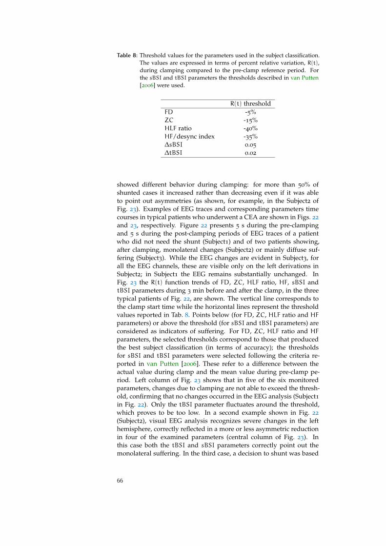
Table 8: Threshold values for the parameters used in the subject classification.The values are expressed in terms of percent relative variation, R(t),during clamping compared to the pre-clamp reference period. Forthe sBSI and tBSI parameters the thresholds described in van Putten[2006] were used.
R(t) thresholdFD -5%ZC -15%HLF ratio -40%HF/desync index -35%∆sBSI 0.05
∆tBSI 0.02
showed different behavior during clamping: for more than 50% ofshunted cases it increased rather than decreasing even if it was ableto point out asymmetries (as shown, for example, in the Subject2 ofFig. 23). Examples of EEG traces and corresponding parameters timecourses in typical patients who underwent a CEA are shown in Figs. 22
and 23, respectively. Figure 22 presents 5 s during the pre-clampingand 5 s during the post-clamping periods of EEG traces of a patientwho did not need the shunt (Subject1) and of two patients showing,after clamping, monolateral changes (Subject2) or mainly diffuse suf-fering (Subject3). While the EEG changes are evident in Subject3, forall the EEG channels, these are visible only on the left derivations inSubject2; in Subject1 the EEG remains substantially unchanged. InFig. 23 the R(t) function trends of FD, ZC, HLF ratio, HF, sBSI andtBSI parameters during 3 min before and after the clamp, in the threetypical patients of Fig. 22, are shown. The vertical line corresponds tothe clamp start time while the horizontal lines represent the thresholdvalues reported in Tab. 8. Points below (for FD, ZC, HLF ratio and HFparameters) or above the threshold (for sBSI and tBSI parameters) areconsidered as indicators of suffering. For FD, ZC, HLF ratio and HFparameters, the selected thresholds correspond to those that producedthe best subject classification (in terms of accuracy); the thresholdsfor sBSI and tBSI parameters were selected following the criteria re-ported in van Putten [2006]. These refer to a difference between theactual value during clamp and the mean value during pre-clamp pe-riod. Left column of Fig. 23 shows that in five of the six monitoredparameters, changes due to clamping are not able to exceed the thresh-old, confirming that no changes occurred in the EEG analysis (Subject1in Fig. 22). Only the tBSI parameter fluctuates around the threshold,which proves to be too low. In a second example shown in Fig. 22
(Subject2), visual EEG analysis recognizes severe changes in the lefthemisphere, correctly reflected in a more or less asymmetric reductionin four of the examined parameters (central column of Fig. 23). Inthis case both the tBSI and sBSI parameters correctly point out themonolateral suffering. In the third case, a decision to shunt was based
66
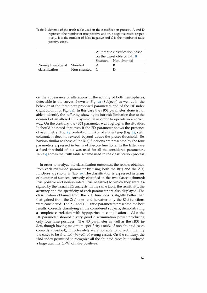
Table 9: Scheme of the truth table used in the classification process. A and Drepresent the number of true positive and true negative cases, respec-tively. B is the number of false negative and C is the number of falsepositive cases.
Automatic classification basedon the thresholds of Tab. 8
Shunted Non-shuntedNeurophysiologist Shunted A Bclassification Non-shunted C D
on the appearance of alterations in the activity of both hemispheres,detectable in the curves shown in Fig. 22 (Subject3) as well as in thebehavior of the three new proposed parameters and of the HF index(right column of Fig. 23). In this case the sBSI parameter alone is notable to identify the suffering, showing its intrinsic limitation due to thedemand of an altered EEG symmetry in order to operate in a correctway. On the contrary, the tBSI parameter well highlights the situation.It should be noted that even if the FD parameter shows the presenceof asymmetry (Fig. 23, central column) or of evident gap (Fig. 23, rightcolumn), it does not exceed beyond doubt the preset threshold. Be-haviors similar to those of the R(t) functions are presented by the fourparameters expressed in terms of Z-score functions. In the latter casea fixed threshold of -1.2 was used for all the considered parameters.Table 9 shows the truth table scheme used in the classification process.
In order to analyze the classification outcomes, the results obtainedfrom each examined parameter by using both the R(t) and the Z(t)functions are shown in Tab. 10. The classification is expressed in termsof number of subjects correctly classified in the two classes (shunted:true positive and non-shunted: true negative) to which they were as-signed by the visual EEG analysis. In the same table, the sensitivity, theaccuracy and the specificity of each parameter are also displayed. Theclassification obtained from the R(t) functions is slightly better thanthat gained from the Z(t) ones, and hereafter only the R(t) functionswere considered. The ZC and HLF ratio parameters presented the bestresults, correctly classifying all the considered subjects, demonstratinga complete correlation with hypoperfusion complications. Also theHF parameter showed a very good discrimination power producingonly four false positives. The FD parameter as well as the sBSI in-dex, though having maximum specificity (100% of non-shunted casescorrectly classified), unfortunately were not able to correctly identifythe cases to be shunted (60-70% of wrong cases). On the contrary, thetBSI index permitted to recognize all the shunted cases but produceda large quantity (25%) of false positives.
67

0 1 2 3 4 5 0 1 2 3 4 5
F4−C4C4−P4P4−O2F8−T6T6−O2F3−C3C3−P3P3−O1F7−T5T5−O1
F4−C4C4−P4P4−O2F8−T6T6−O2F3−C3C3−P3P3−O1F7−T5T5−O1
F4−C4C4−P4P4−O2F8−T6T6−O2F3−C3C3−P3P3−O1F7−T5T5−O1
time [s]PRE−CLAMP POST−CLAMP
Subject1
Subject2
Subject3
Figure 22: Five seconds of EEG traces during pre- (left column) and post-clamp (right column) periods in three typical patients present-ing no changes (Subject1), monolateral differences (Subject2), andmainly diffuse suffering (Subject3). Subject1 was not shunted whilethe remaining two were shunted.
68
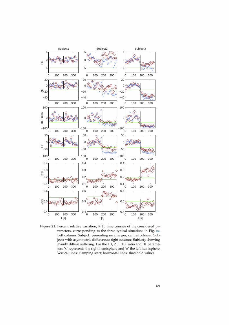
0 100 200 3000.4
0.5
0.6
t [s]
sBS
I
0 100 200 3000.1
0.2
0.3
0.4
tBS
I
0 100 200 300
−5
0
5Subject1
FD
0 100 200 300
−40
−20
0
20
ZC
0 100 200 300−100
−50
0
50
HF
0 100 200 300−100
0
100
HLF
rat
io
0 100 200 3000.4
0.5
0.6
t [s]
0 100 200 3000.1
0.2
0.3
0.4
0 100 200 300
−5
0
5Subject2
0 100 200 300
−40
−20
0
20
0 100 200 300−100
−50
0
50
0 100 200 300−100
0
100
0 100 200 3000.4
0.5
0.6
t [s]
0 100 200 3000.1
0.2
0.3
0.4
0 100 200 300
−5
0
5Subject3
0 100 200 300
−40
−20
0
20
0 100 200 300−100
−50
0
50
0 100 200 300−100
0
100
Figure 23: Percent relative variation, R(t), time courses of the considered pa-rameters, corresponding to the three typical situations in Fig. 22.Left column: Subject1 presenting no changes; central column: Sub-ject2 with asymmetric differences; right column: Subject3 showingmainly diffuse suffering. For the FD, ZC, HLF ratio and HF parame-ters ’x’ represents the right hemisphere and ’o’ the left hemisphere.Vertical lines: clamping start; horizontal lines: threshold values.
69
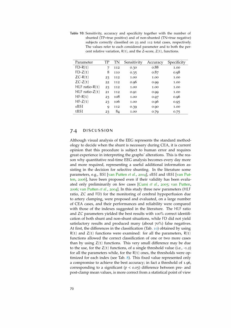
Table 10: Sensitivity, accuracy and specificity together with the number ofshunted (TP=true positive) and of non-shunted (TN=true negative)subjects correctly classified on 23 and 112 total cases, respectively.The values refer to each considered parameter and to both the per-cent relative variation, R(t), and the Z-score, Z(t), functions.
Parameter TP TN Sensitivity Accuracy SpecificityFD-R(t) 7 112 0.30 0.88 1.00
FD-Z(t) 8 110 0.35 0.87 0.98
ZC-R(t) 23 112 1.00 1.00 1.00
ZC-Z(t) 22 112 0.96 0.99 1.00
HLF ratio-R(t) 23 112 1.00 1.00 1.00
HLF ratio-Z(t) 21 112 0.91 0.99 1.00
HF-R(t) 23 108 1.00 0.97 0.96
HF-Z(t) 23 106 1.00 0.96 0.95
sBSI 9 112 0.39 0.90 1.00
tBSI 23 84 1.00 0.79 0.75
7.4 discussionAlthough visual analysis of the EEG represents the standard method-ology to decide when the shunt is necessary during CEA, it is currentopinion that this procedure is subject to human error and requiresgreat experience in interpreting the graphs’ alterations. This is the rea-son why quantitative real-time EEG analysis becomes every day moreand more required, representing a useful additional information as-sisting in the decision for selective shunting. In the literature someparameters, e.g., BSI [van Putten et al., 2004], sBSI and tBSI [van Put-ten, 2006], have been proposed even if their validity has been evalu-ated only preliminarily on few cases [Cursi et al., 2005; van Putten,2006; van Putten et al., 2004]. In this study three new parameters (HLFratio, ZC and FD) for the monitoring of cerebral hypoperfusion dueto artery clamping, were proposed and evaluated, on a large numberof CEA cases, and their performances and reliability were comparedwith those of the indexes suggested in the literature. The HLF ratioand ZC parameters yielded the best results with 100% correct identifi-cation of both shunt and non-shunt situations, while FD did not yieldsatisfactory results and produced many (about 70%) false negatives.At first, the differences in the classification (Tab. 10) obtained by usingR(t) and Z(t) functions were examined: for all the parameters, R(t)functions allowed the correct classification of one or two more casesthan by using Z(t) functions. This very small difference may be dueto the use, for the Z(t) functions, of a single threshold value (i.e., -1.2)for all the parameters while, for the R(t) ones, the thresholds were op-timized for each index (see Tab. 8). This fixed value represented onlya compromise to achieve the best accuracy; in fact a threshold of 1.96,corresponding to a significant (p < 0.05) difference between pre- andpost-clamp mean values, is more correct from a statistical point of view
70
but is inappropriate for a good classification. However, the Z(t) func-tions are also influenced by the signal variability and consequently bythe noise present on the EEG: more noise produces larger variance andsmaller Z(t) changes, making harder to exceed the threshold. Anotherremark concerns the EEG derivations used in the parameter calcula-tion: even if some authors [Laman et al., 2012] suggest to use selectedderivations because of their higher sensitivity in detection of anoma-lies occurring during carotid surgery than others, in this work goodresults were also obtained using equally weighted bipolar EEG chan-nels; consequently, a channel selection was not considered necessary.A main result of this work is to show that the R(t) functions of two ofthe new examined parameters, i.e., the ZC and the HLF ratio, were ableto correctly identify all cases presenting either mono- (asymmetric) orbilateral (diffuse) hemispherical suffering (as suggested by visual EEGanalysis). In these cases the left and right R(t) time courses presented,for no less than 30 s, a significant decrease below a threshold of -15%,for ZC, and of -40%, for the HLF ratio, of the pre-clamp mean values,thus providing precise indications of possible cerebral ischemia. In ad-dition, the two parameters were also able to correctly discriminate allthe cases in which the shunt was not required, corresponding to nosignificant EEG changes, showing they could capture EEG variationsdue to any kind of intra- or interhemispheric suffering. Furthermore,the simultaneous use of two R(t) curves, one for each EEG side, per-mits to immediately identify possible asymmetries present in the EEGchanges during CEA.
The HLF ratio was based on the hypothesis, described in the litera- HLF ratio
ture [Blume et al., 1986; Minicucci et al., 2000; Salvian et al., 2012], thatalpha and beta EEG spectral powers decrease in presence of brain hy-poperfusion followed by an increase of delta power, the latter beingfrequently not significant. Based on a similar idea, but limited onlyto the alpha and beta bands, Cursi et al. [2005] suggested the desyn-chronization index (corresponding in this study to the R(t) functionof the HF parameter). As reported in the results, the HF was able tocorrectly identify all the subjects to be shunted and only four casesof non-shunted patients were wrongly classified. Moreover, the opti-mal threshold value found in this study for the HF index is the samesuggested in [Cursi et al., 2005]. Adding the information coming fromlower frequencies (0.5-5 Hz band), used as the denominator in the HLFratio parameter, improves the HF performance: exact subject classifica-tion is achieved. This work confirms that the 8-15 Hz frequency rangeis the band which is most sensitive to possible cerebral suffering dur-ing CEA [Cursi et al., 2005; Minicucci et al., 2000]. Moreover, the resultssupport the hypothesis that the utilization of the information includedinto the 0.5ñ5 Hz band may slightly improve the specificity, producinga more accurate identification of the cases that do not require shunting.
The ZC parameter, recently proposed for studying dementia, sleep- Zero-crossings
stage characteristics and background activity [Carrozzi et al., 2004; Hen-derson et al., 2006; Lin et al., 2006] from EEG series, turned out to becapable of sensing reduction of fast activity as well as possible slow
71
activity changes, thus producing an indicator that can assist in the de-cision whether to proceed with shunting during CEA. The ZC param-eter, measuring possible dominant frequency (or band) modifications,proved to be strongly correlated with the visual assessment of the EEGchanges due to brain suffering. It is underlined that the ZC parameteris very easily calculated directly from temporal signals and it does notrequire power spectrum evaluation of the EEG (as the HLF ratio or theHF index do). Hence, it is suitable for a real time implementation andits time course, added as a further signal in the visualization of theEEG derivations, may permit the successful outcome of the surgicalprocedure.
The third examined new parameter, FD, did not yield satisfactoryFractal dimension
results. It produced many (about 70%) false negatives (i.e., it did notidentify many subjects to be shunted), even if it correctly recognized allthe subjects that did not need shunting. This situation was mainly dueto an uncertain decrement of the FD values in many cases of cerebralhypoperfusion: the FD changes were too small and an increase of thethreshold value produced a very large increment of false positive cases.The FD parameter, measuring the fractal behavior of the EEG signal,was not able to recognize generalized EEG decreases, since it does notchange if the signal is merely rescaled in amplitude; thus it producedmany classification errors. Furthermore, the EEG complexity changessensed by the FD were so small they did not exceed the threshold.
The sBSI parameter produced slightly better results than FD. ThesBSI
index corresponds to the previously proposed [van Putten et al., 2004]brain symmetry index (BSI) and it should quantify hemispheric changesin spectral symmetry. Unfortunately, the sBSI index excluded about60% of the subjects to be shunted (false negative), confirming the limitsalready underlined by [van Putten, 2006] even if on a limited numberof cases (4). In fact, the sBSI parameter was able to detect only thecases presenting asymmetric spatial changes in the EEG, showing onthe contrary insensitivity to distributed attenuation of fast activity orto diffuse increase of delta activity.
In order to overcome this limitation and to be also sensitive to tem-tBSI
poral changes in spectral characteristics, a further index (tBSI) wasproposed by van Putten [2006]. The tBSI index yielded 28 wronglyclassified cases, on a total of 112 (25% of false positive), suggestingshunt when it was not necessary. It should be noted that the combineduse of the sBSI and tBSI indexes did not improve the results; prob-ably both sBSI and tBSI parameters are able to identify asymmetricchanges. It is evident that the equation 33 used by van Putten couldbe not sufficient to cancel the influence of spatial asymmetries on tBSI,or (alternatively but improbably) all the cases here considered show-ing asymmetry also included diffuse EEG changes sensed by the tBSIparameter. However, in all the examined subjects the tBSI index aloneproduced the same classification result as when used with the sBSIcontribution. Furthermore, since the tBSI index calculation considersthe absolute value of the pre/post-clamp difference (Eq. 34), it is mod-ified not only by a signal decrease but also by a signal increase that
72
generally indicates activation [Visser et al., 1999], as it could happenwhen the haematic flow increases or anesthesia becomes less deep.This situation is signaled by the tBSI parameter as a need of shuntwhen it is actually not required; this fact could explain some of thefalse positives obtained with this index.
7.5 conclusionSince routine shunting may increase the risk of perioperative stroke[Salvian et al., 2012], EEG monitoring, based on quantitative measuresof the EEG changes, proved to be a useful tool for shunt decision dur-ing CEA. In this study the R(t) functions of some new parameters,in particular the HLF ratio and the ZC indexes, showed to be ableto correctly identify cases presenting mono- or bilateral hemisphericchanges capturing both asymmetric and diffuse suffering situations.As proved by the retrospective analysis, in those patients where themean value of the HLF ratio or the ZC parameters go below -40%and -15% thresholds, respectively, in the 3 min before clamping, visualEEG analysis showed significant changes, and shunting was advised.Slightly worse results (4% of false positives) had been achieved withthe HF/desynchronization index (previously proposed by Cursi et al.[2005]) while the pair of sBSI/tBSI parameters (or the tBSI alone) pro-duced about 25% of false positives. Finally, the FD parameter and thesBSI index alone did not yield good results, and generated large clas-sification errors. In conclusion, the R(t) function of the ZC parameterrepresents the best choice both for a correct classification and for thepossibility of real-time implementation. The contemporary utilizationof the R(t) left and right functions permits an immediate quantificationof possible asymmetries as well as, when used as continuous displaybeside the EEG derivations, the identification of EEG changes due toartifacts or anesthesia. Thus, the Author proposes to use the ZC param-eter to support the visual assessment of the EEG during CEA, offeringa quantitative measure for EEG alterations due to cerebral hypoperfu-sion.
73

8 M O N I TO R I N G T H E D E P T HO F A N E S T H E S I A
contents8.1 Introduction and motivation 758.2 Material and Methods 77
8.2.1 Patients 77
8.2.2 EEG recording and analysis 77
8.3 Results 788.4 Discussion 808.5 Conclusion 84
The assessment of the depth of anesthesia based on the analysis ofthe EEG is an active field of research. Although many methods, in-cluding BISTMsystem, have been developed over the years to quantifyunconsciousness during anesthesia, intraoperative awareness is still amajor clinical problem. This chapter explores an alternative approach,based on the nonlinear analysis of the EEG, aimed at reducing both theincidence of intraoperative awareness and the computational complex-ity of BIS. The standalone fractal dimension (FD) and zero-crossings(ZC), as well as the burst suppression compensated FD (bsFD) and ZC(bsZC), as measures of the depth of anesthesia, are evaluated in thispreliminary study and compared with BIS index. The chapter is basedon Author’s publication 5.
8.1 introduction and motivationThe monitoring of anesthesia based on EEG parameterization is in-tended to help anesthesiologists maintain suitable level of hypnosis inorder to provide optimal working conditions to surgeons and to ensurepatient’s safety. While, on the one hand, too deep anesthesia must beavoided in order to prevent over dosing side effects, on the other hand,low doses of hypnotic agents can cause some form of intraoperativeawareness. In this situation patients may hear conversations, have vi- Intraoperative
awarenesssual perceptions, feel pressure or pain and be unable to communicatetheir sensations [Schwender et al., 1998]. After operation, patients canrecall all of the details of the procedure and can experience unpleasantfurther effects like anxiety, sleep loss, nightmares and panic attacks.A severe anxiety disorder, namely the post-traumatic stress disorder(PTSD), can develop as a result of these postoperative effects [Jones,1994; Osterman et al., 2001].
Several depth-of-hypnosis assessment methods, based on linear and State of the art
nonlinear measures of the EEG, have been proposed in the last decade
75

to provide a quantitative objective measure of the depth of anesthe-sia. Multiscale rescaled range analysis [Liang et al., 2011], wavelet-based bicoherence [Li et al., 2011], spectral entropy [Ferenets et al., 2007;Klockars et al., 2011], approximate entropy and Lempel-Ziv complex-ity [Jordan et al., 2006] are mentioned as examples. Some commercialsystems, based on the Patient State Index (PSI) [Drover et al., 2002], theNarcotrend monitoring [Kreuer et al., 2003] and the EntropyTMmethod[Viertiö-Oja et al., 2004] have been recently introduced in the operat-ing room. The benchmark comparator for all these monitors is theBISTMindex
Bispectral Index Score BISTM of Aspect Medical Systems (Newton,MA) [Kelley, 2010]. Bispectral index is a parameter that integratesseveral electroencephalographic measures into a unit-less number be-tween 100 (fully awake) and 0 (flat line EEG). Although the exact al-gorithm used to synthesize the index is still unknown, some studiesreferenced in Morimoto et al. [2004] brought new insight into the BIS-calculation process. After artifacts removal, the EEG is firstly analyzedfor suppression detection and quantification through the burst sup-pression ratio. Then the signal is fast Fourier transformed (FFT) tocompute a relative beta ratio and to derive the bispectrum, from whichthe relative synchrony of fast and slow waves is calculated. These pa-rameters are combined to generate the BIS index, whose values, up-dated every second, should be maintained within the recommendedrange (40 to 60) for patient safety during surgery.
Despite the use of such monitors, the incidence of awareness duringRationale
general anesthesia that can be recalled explicitly after operation hasbeen reported to be 1.1% in total intravenous anesthesia (TIVA) and0.59% in balanced anesthesia [Errando et al., 2008]. Sometimes anesthe-siologists have to rely on objective autonomic measures such as heartrate, blood pressure, respiration pattern and body temperature [Miller,2005] or even on subjective assessments based, for example, on theRamsay sedation scale [Ramsay et al., 2012]. For this reason, researchin the field of EEG-based monitoring of anesthesia is still very active.
The present study proposes an alternative methodology with theAdopted approach
twofold aim of minimizing the incidence of intraoperative awarenessand reducing the computational complexity of BIS [Miller et al., 2004;Schneider et al., 2004]. Two nonlinear indexes, the fractal dimension(FD) and the zero-crossings (ZC), are off-line calculated and then com-bined with the burst suppression ratio (BSR) to produce the bsFD andbsZC indexes. The indexes, proposed to monotonically quantify thedepth of anesthesia, are compared with BIS by means of Pearson’s cor-relation analysis. The comparison with BIS is made also in terms ofability to detect the onset of possible awareness.
76

Figure 24: The BIS sensorTMused for the recording of both BIS and raw EEG.
8.2 material and methods
8.2.1 Patients
The methodology proposed in the present research was applied toEEG recordings from 6 patients who underwent surgery under generalanesthesia. The study was approved by the Ethics Committee of theIRCCS “Burlo Garofolo” Scientific Institute of Trieste. General anes-thesia was induced by intravenous propofol (hypnotic agent), fentanyl(analgesic) and rocuronium/vecuronium (muscle relaxants). Anesthesiawas maintained, under BIS control, by administration of inhalationalagent sevoflurane (balanced anesthesia, 4 patients) or propofol (total in-travenous anesthesia, 2 patients). Some patients were premedicatedwith 1-2 mg of midazolam.
8.2.2 EEG recording and analysis
In order to minimally interfere with the standard surgical procedure, Recording
the BIS sensorTM(Aspect Medical Systems, Newton, MA), applied tothe forehead of the patients before the induction of anesthesia, wasused to acquire both the BIS index and raw EEG data (Fig. 24). The ac-quisition started at least 2 minutes before the induction of the hypnoticagent in order to have a baseline for the successive evaluations. At theend of the surgical procedure data were transferred from the BIS Mon-itor to a laptop computer via USB. EEG signals were A/D convertedwith a sampling frequency of 128 Hz, according to the guidelines ofChapter 5, and 16-bit accuracy. The EEG derivation selected for the Pre-processing
analysis corresponds to the Fp1-Fpz bipolar derivation of the 10-20 sys-
77
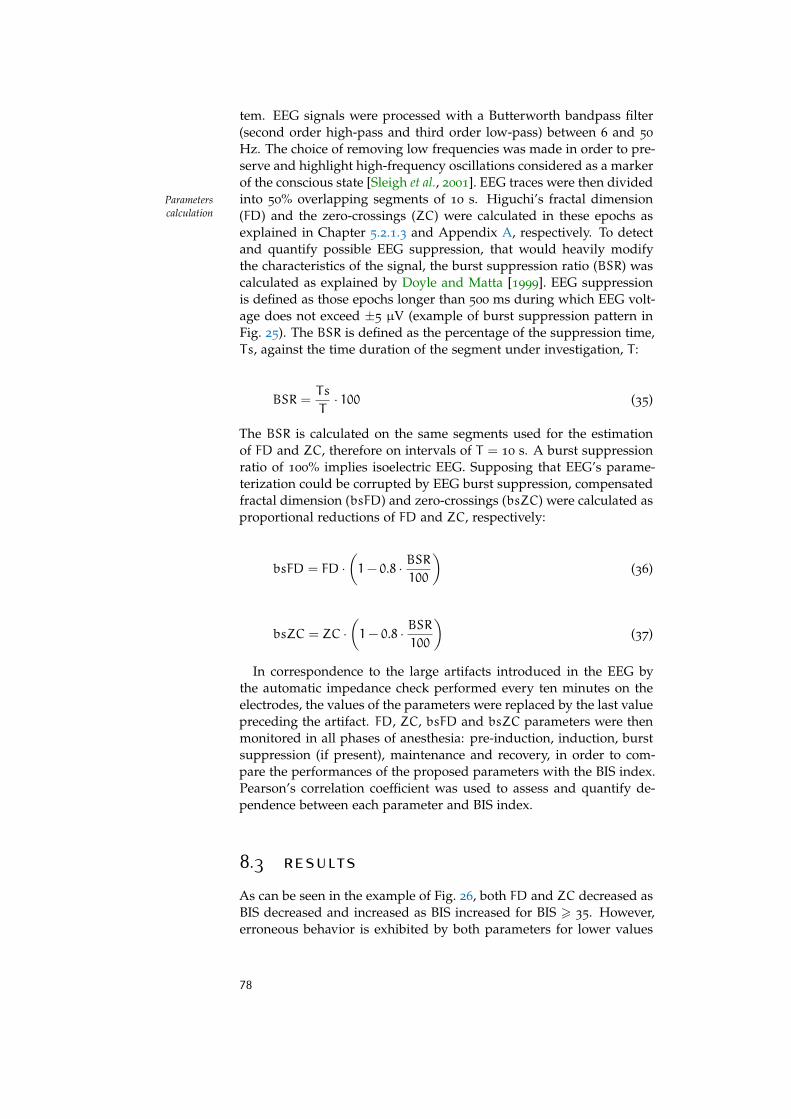
tem. EEG signals were processed with a Butterworth bandpass filter(second order high-pass and third order low-pass) between 6 and 50
Hz. The choice of removing low frequencies was made in order to pre-serve and highlight high-frequency oscillations considered as a markerof the conscious state [Sleigh et al., 2001]. EEG traces were then dividedinto 50% overlapping segments of 10 s. Higuchi’s fractal dimensionParameters
calculation (FD) and the zero-crossings (ZC) were calculated in these epochs asexplained in Chapter 5.2.1.3 and Appendix A, respectively. To detectand quantify possible EEG suppression, that would heavily modifythe characteristics of the signal, the burst suppression ratio (BSR) wascalculated as explained by Doyle and Matta [1999]. EEG suppressionis defined as those epochs longer than 500 ms during which EEG volt-age does not exceed ±5 µV (example of burst suppression pattern inFig. 25). The BSR is defined as the percentage of the suppression time,Ts, against the time duration of the segment under investigation, T :
BSR =Ts
T· 100 (35)
The BSR is calculated on the same segments used for the estimationof FD and ZC, therefore on intervals of T = 10 s. A burst suppressionratio of 100% implies isoelectric EEG. Supposing that EEG’s parame-terization could be corrupted by EEG burst suppression, compensatedfractal dimension (bsFD) and zero-crossings (bsZC) were calculated asproportional reductions of FD and ZC, respectively:
bsFD = FD ·(1− 0.8 · BSR
100
)(36)
bsZC = ZC ·(1− 0.8 · BSR
100
)(37)
In correspondence to the large artifacts introduced in the EEG bythe automatic impedance check performed every ten minutes on theelectrodes, the values of the parameters were replaced by the last valuepreceding the artifact. FD, ZC, bsFD and bsZC parameters were thenmonitored in all phases of anesthesia: pre-induction, induction, burstsuppression (if present), maintenance and recovery, in order to com-pare the performances of the proposed parameters with the BIS index.Pearson’s correlation coefficient was used to assess and quantify de-pendence between each parameter and BIS index.
8.3 resultsAs can be seen in the example of Fig. 26, both FD and ZC decreased asBIS decreased and increased as BIS increased for BIS > 35. However,erroneous behavior is exhibited by both parameters for lower values
78
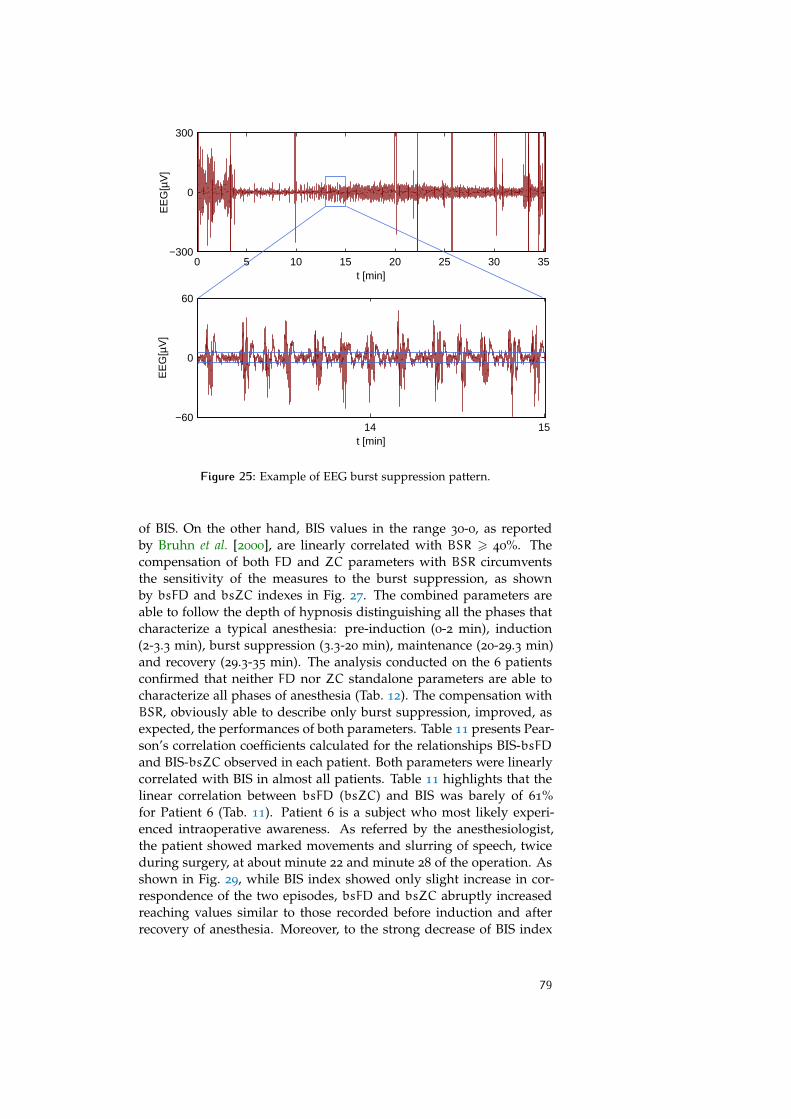
0 5 10 15 20 25 30 35−300
0
300
t [min]
EE
G[µ
V]
14 15−60
0
60
t [min]
EE
G[µ
V]
Figure 25: Example of EEG burst suppression pattern.
of BIS. On the other hand, BIS values in the range 30-0, as reportedby Bruhn et al. [2000], are linearly correlated with BSR > 40%. Thecompensation of both FD and ZC parameters with BSR circumventsthe sensitivity of the measures to the burst suppression, as shownby bsFD and bsZC indexes in Fig. 27. The combined parameters areable to follow the depth of hypnosis distinguishing all the phases thatcharacterize a typical anesthesia: pre-induction (0-2 min), induction(2-3.3 min), burst suppression (3.3-20 min), maintenance (20-29.3 min)and recovery (29.3-35 min). The analysis conducted on the 6 patientsconfirmed that neither FD nor ZC standalone parameters are able tocharacterize all phases of anesthesia (Tab. 12). The compensation withBSR, obviously able to describe only burst suppression, improved, asexpected, the performances of both parameters. Table 11 presents Pear-son’s correlation coefficients calculated for the relationships BIS-bsFDand BIS-bsZC observed in each patient. Both parameters were linearlycorrelated with BIS in almost all patients. Table 11 highlights that thelinear correlation between bsFD (bsZC) and BIS was barely of 61%for Patient 6 (Tab. 11). Patient 6 is a subject who most likely experi-enced intraoperative awareness. As referred by the anesthesiologist,the patient showed marked movements and slurring of speech, twiceduring surgery, at about minute 22 and minute 28 of the operation. Asshown in Fig. 29, while BIS index showed only slight increase in cor-respondence of the two episodes, bsFD and bsZC abruptly increasedreaching values similar to those recorded before induction and afterrecovery of anesthesia. Moreover, to the strong decrease of BIS index
79
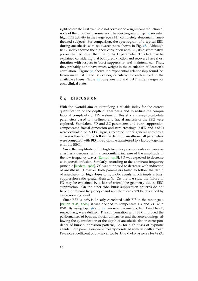
right before the first event did not correspond a significant reduction ofnone of the proposed parameters. The spectrogram of Fig. 30 revealedhigh EEG activity in the range 15-48 Hz, completely abnormal in anes-thetized subjects. For comparison, the spectrogram of a typical EEGduring anesthesia with no awareness is shown in Fig. 28. AlthoughbsZC index showed the highest correlation with BIS, its discriminativepower resulted lower than that of bsFD parameter. This fact may beexplained considering that both pre-induction and recovery have shortduration with respect to burst suppression and maintenance. Thus,they probably don’t have much weight in the calculation of Pearson’scorrelation. Figure 31 shows the exponential relationship found be-tween mean bsFD and BIS values, calculated for each subject in theavailable phases. Table 13 compares BIS and bsFD index ranges foreach clinical state.
8.4 discussionWith the twofold aim of identifying a reliable index for the correctquantification of the depth of anesthesia and to reduce the compu-tational complexity of BIS system, in this study 4 easy-to-calculateparameters based on nonlinear and fractal analysis of the EEG wereexplored. Standalone FD and ZC parameters and burst suppressioncompensated fractal dimension and zero-crossings (bsFD and bsZC)were evaluated on 6 EEG signals recorded under general anesthesia.To assess their ability to follow the depth of anesthesia, all parameterswere compared with BIS index, off-line transferred to a laptop togetherwith the EEG.
Since the amplitude of the high frequency components decreases asanesthesia deepens, with a concomitant increase of the amplitude ofthe low frequency waves [Rampil, 1998], FD was expected to decreasewith propofol infusion. Similarly, according to the dominant frequencyprinciple [Kedem, 1986], ZC was supposed to decrease with inductionof anesthesia. However, both parameters failed to follow the depthof anesthesia for high doses of hypnotic agents which imply a burstsuppression ratio greater than 40%. On the one side, the failure ofFD may be explained by a loss of fractal-like geometry due to EEGsuppression. On the other side, burst suppression patterns do nothave a dominant frequency/band and therefore can’t be described byzero-crossings count.
Since BSR > 40% is linearly correlated with BIS in the range 30-0[Bruhn et al., 2000], it was decided to compensate FD and ZC withBSR. By using Eqs. 36 and 37 two new parameters, bsFD and bsZC,respectively, were defined. The compensation with BSR improved theperformances of both the fractal dimension and the zero-crossings, al-lowing the quantification of the depth of anesthesia also in correspon-dence of burst suppression patterns, i.e., for high doses of hypnoticagents. Both parameters were linearly correlated with BIS with a meanPearson’s coefficient of 0.75±0.11 for bsFD and of 0.79 ±0.11 for bsZC.
80
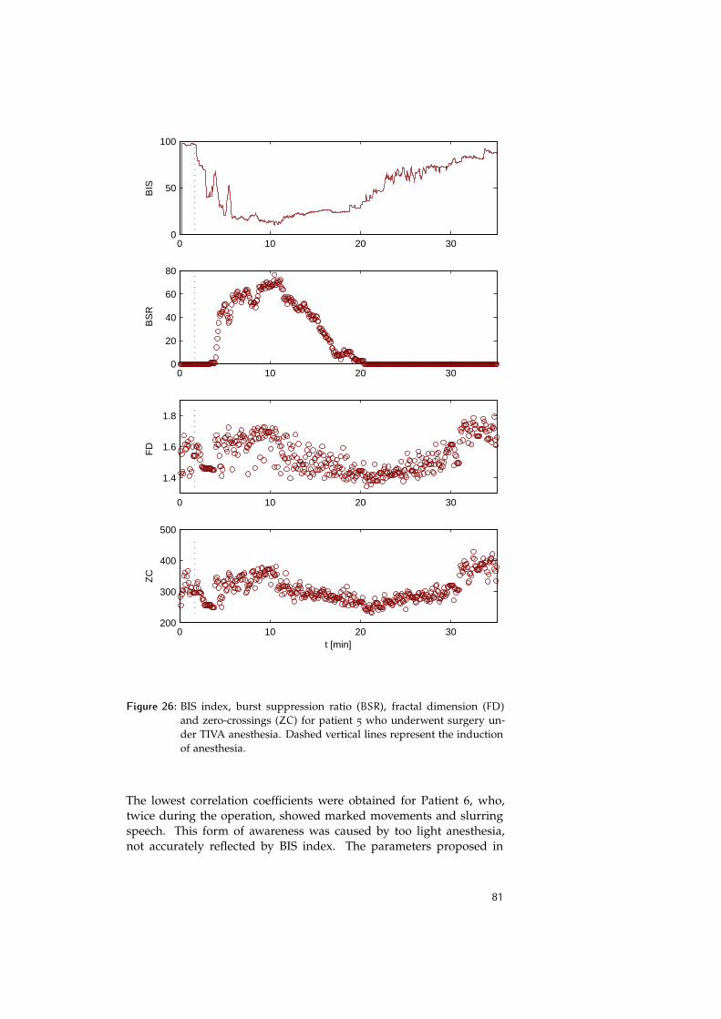
0 10 20 30
1.4
1.6
1.8
FD
0 10 20 30200
300
400
500
ZC
t [min]
0 10 20 300
50
100B
IS
0 10 20 300
20
40
60
80
BS
R
Figure 26: BIS index, burst suppression ratio (BSR), fractal dimension (FD)and zero-crossings (ZC) for patient 5 who underwent surgery un-der TIVA anesthesia. Dashed vertical lines represent the inductionof anesthesia.
The lowest correlation coefficients were obtained for Patient 6, who,twice during the operation, showed marked movements and slurringspeech. This form of awareness was caused by too light anesthesia,not accurately reflected by BIS index. The parameters proposed in
81
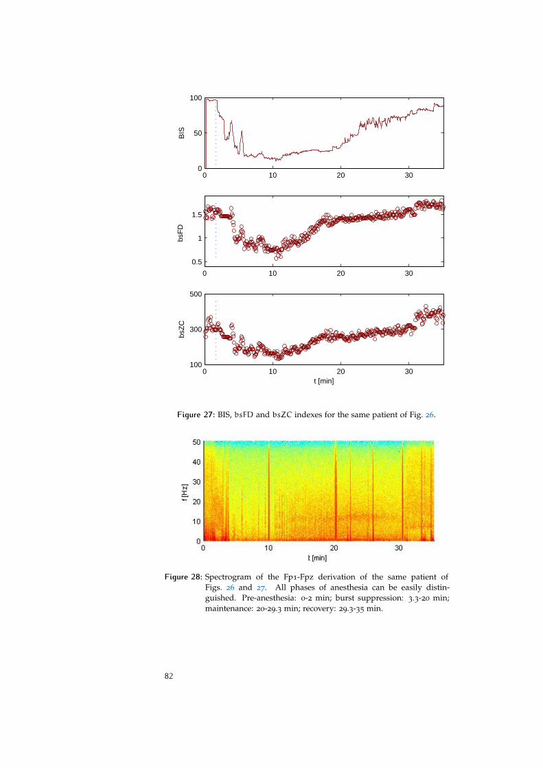
0 10 20 30
0.5
1
1.5
bsF
D
0 10 20 30100
300
500
bsZ
C
t [min]
0 10 20 300
50
100
BIS
Figure 27: BIS, bsFD and bsZC indexes for the same patient of Fig. 26.
Figure 28: Spectrogram of the Fp1-Fpz derivation of the same patient ofFigs. 26 and 27. All phases of anesthesia can be easily distin-guished. Pre-anesthesia: 0-2 min; burst suppression: 3.3-20 min;maintenance: 20-29.3 min; recovery: 29.3-35 min.
82
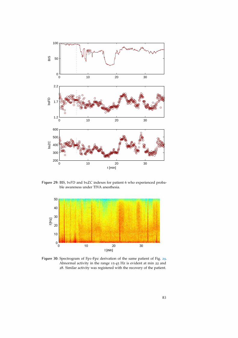
0 10 20 301.2
1.7
2.2
bsF
D
0 10 20 30200
300
400
500
600
bsZ
C
t [min]
0 10 20 300
50
100
BIS
Figure 29: BIS, bsFD and bsZC indexes for patient 6 who experienced proba-ble awareness under TIVA anesthesia.
Figure 30: Spectrogram of Fp1-Fpz derivation of the same patient of Fig. 29.Abnormal activity in the range 15-45 Hz is evident at min 22 and28. Similar activity was registered with the recovery of the patient.
83

Table 11: Pearson’s correlation coefficients between BIS and both bsFD andbsZC parameters.
BIS-bsFD BIS-bsZCPatient1 0.88 0.89
Patient2 0.71 0.77
Patient3 0.77 0.84
Patient4 0.64 0.75
Patient5 0.87 0.89
Patient6 0.61 0.61
Table 12: Ability to distinguish among the different phases of anesthesia ofthe considered parameters.
pre-anesthesia burst suppression maintenance recoveryBSR
√
FD√ √ √
ZC√
bsFD√ √ √ √
bsZC√ √
this study, on the contrary, clearly increased in correspondence to bothepisodes (Fig. 29). The analysis of the spectrogram (Fig. 30) confirmedthe presence of abnormal high activity in the range 15-48 Hz, whichreflects changes in the conscious state [Sleigh et al., 2001]. As can beseen in the spectrogram of a successful anesthesia (Fig. 28), mainte-nance is characterized by the presence of a 13 Hz oscillation with nohigh frequency activity observed.
One trend revealed by this preliminary study is the high variabilityof the proposed indexes in the pre-anesthesia phase. The reason forthis behavior may be related to the concomitant administration of dif-ferent drugs. Further investigations should attempt to clarify the causeof this variability since a more stable baseline is desirable.
Although bsZC had the highest correlation with BIS, the index thatyielded the best results discriminating among all possible levels of se-dation was bsFD. This information warrants further investigations tobetter establish whether bsFD or bsZC represents the most reliablemonitoring tool. In any case, the power of the proposed parameterslies in the ability of reflecting changes occurring both in the low spec-trum and in the high frequency range, though calculated directly inthe time domain.
84
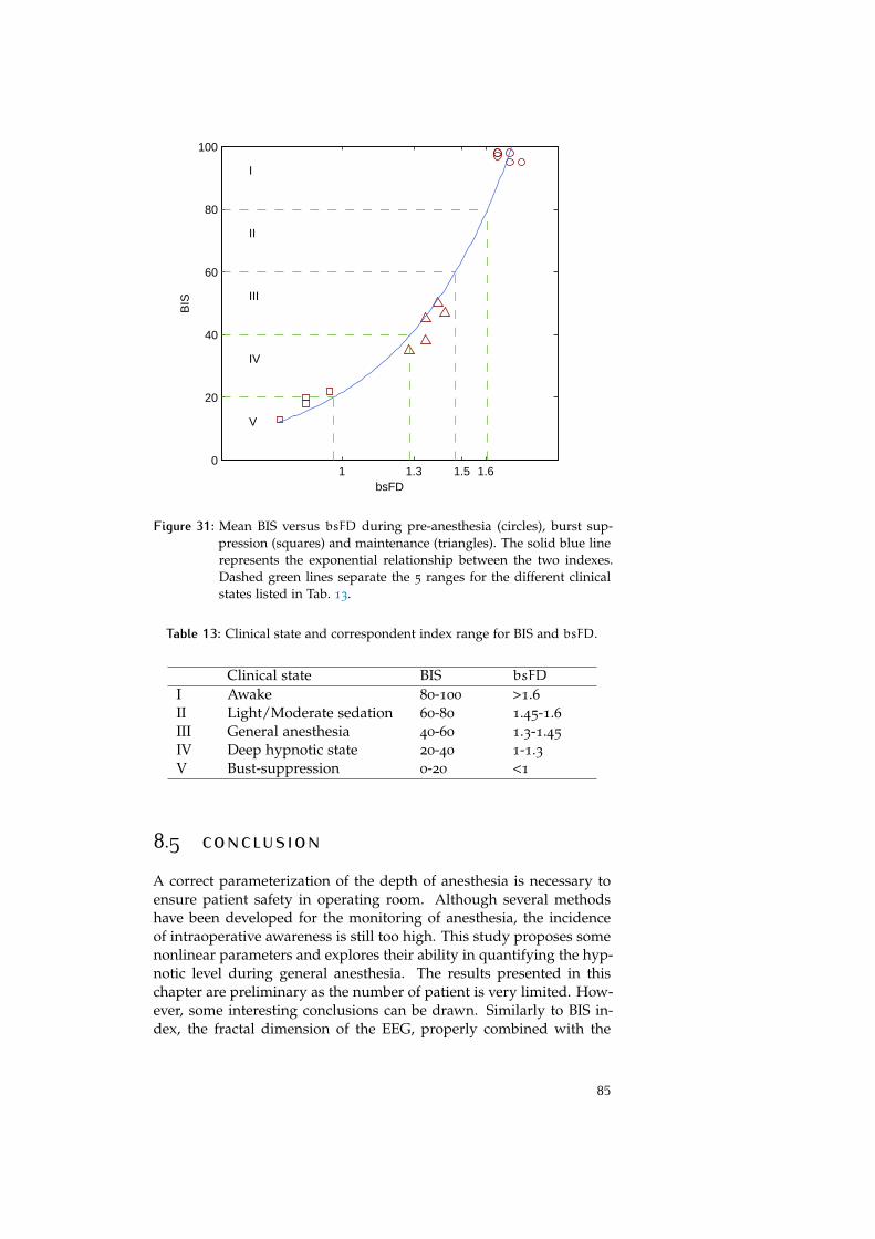
1 1.3 1.5 1.60
20
40
60
80
100
bsFD
BIS
IV
V
III
II
I
Figure 31: Mean BIS versus bsFD during pre-anesthesia (circles), burst sup-pression (squares) and maintenance (triangles). The solid blue linerepresents the exponential relationship between the two indexes.Dashed green lines separate the 5 ranges for the different clinicalstates listed in Tab. 13.
Table 13: Clinical state and correspondent index range for BIS and bsFD.
Clinical state BIS bsFD
I Awake 80-100 >1.6II Light/Moderate sedation 60-80 1.45-1.6III General anesthesia 40-60 1.3-1.45
IV Deep hypnotic state 20-40 1-1.3V Bust-suppression 0-20 <1
8.5 conclusion
A correct parameterization of the depth of anesthesia is necessary toensure patient safety in operating room. Although several methodshave been developed for the monitoring of anesthesia, the incidenceof intraoperative awareness is still too high. This study proposes somenonlinear parameters and explores their ability in quantifying the hyp-notic level during general anesthesia. The results presented in thischapter are preliminary as the number of patient is very limited. How-ever, some interesting conclusions can be drawn. Similarly to BIS in-dex, the fractal dimension of the EEG, properly combined with the
85
burst suppression ratio, is able to monitor the depth of anesthesia dis-tinguishing among all different clinical states (Fig. 31 and Tab. 13).Moreover, bsFD index detects two episodes of intraoperative aware-ness whose onset was not clearly indicated by BIS monitor. The pro-posed parameter, combination of two time domain measures, is of lowcomputational cost and therefore more suitable for real-time imple-mentation. Should such preliminary results be confirmed on a largersample, anesthesiologists could be provided with an easy-to-calculatereliable index for the monitoring of the depth of anesthesia and thereduction of the incidence of intraoperative awareness.
86
9 M A C R O -S T R U C T U R A L E E GO R G A N I Z AT I O N I N A U T I S M
contents9.1 Introduction and motivation 879.2 Materials and Methods 89
9.2.1 Patients 89
9.2.2 EEG recording and analysis 89
9.3 Results 919.4 Discussion 989.5 Conclusion 99
The characterization of the macro-structural organization of the EEGin autism, with respect to that of mental retardation, has not been pre-viously studied. Some preliminary investigations have been conductedto differentiate autistic and normal electroencephalographic activity.However, most of the studies carried on the autistic EEG principallyaimed at analyzing the co-occurrence of autism and epilepsy. In thischapter the problem of autistic macro-structural neuronal organizationis addressed through linear and nonlinear quantitative analysis of theEEG recorded in the three major electrical states: awake state, lightsleep (stages 1 and 2) and deep sleep (stages 3 and 4). A statisticalanalysis is performed in order to identify the measures the best dis-criminate between the populations of autistic children and childrenwith mental retardation. The chapter is based on Author’s publication6.
9.1 introduction and motivationAutism is defined as a behavioral, cognitive and brain developmental Autism
disorder characterized by impairments in social interaction and com-munication, as well as by the presence of restricted and repetitive be-haviors, interests and activities [Rapin, 1997]. Abnormalities in grossbrain structure, neuronal growth patterns, abnormal connectivity andneurotransmitter profiles have been extensively studied [Belmonte etal., 2004; Penn, 2006; Rippon et al., 2007]. The study of the autistic brainhas been approached with different investigation techniques such asEEG, MEG, magnetic resonance imaging (MRI) and functional MRI(fMRI) [Mengotti et al., 2011; Philip et al., 2012; Wilson et al., 2007]. Thesearch for objective measures that can help in screening for autisticchildren is of primary importance since, till now, most of the toolsavailable to physicians rely on subjective observations. Autism be-longs to the autism spectrum disorders (ASD), a broad classification
87
that includes also Asperger’s Syndrome and pervasive developmentaldisorder not otherwise specified. Moreover, overlap among other be-havioral and developmental disorders can produce false positives andsubsequently poor test specificity. A correct early diagnosis wouldimprove treatment and patient’s longterm quality of life.
The EEG represents a promising diagnosis tool, since it providesState of the art
a low-cost description of brain activity dynamics with high temporalresolution. To date, most of the studies based on the EEG addressthe problem of the co-occurrence of autism and epilepsy [Tuchmanet al., 2010]. However, some investigations aimed at the characteri-zation of autistic brain activity, with no reference to epileptic abnor-malities, have been recently published. On the basis of conventionallinear analysis, Grice et al. [2001] observed higher power for gammasub-band of autistic EEG when compared with non-ASD signals. Onthe other hand, Chan et al. [2009] reported a significant reduction oftheta activity in the anterior regions of the brain, while the resultspresented by Pop-Jordanova et al. [2010] indicated increased delta andtheta power in the frontal derivations. However, the highly nonlinearand complex dynamics of the brain, brought to light in the last fewdecades, may not be exhaustively explained by traditional linear tech-niques. For this reason, chaos theory and fractal analysis have beenrecently introduced in ASD research as tools for the study of autis-tic brain features from a nonlinear perspective. Ahmadlou et al. [2010]recently proposed an automated EEG-based diagnosis methodologywhich combines wavelet decomposition, fractal analysis and neuralnetworks. In the study of Catarino et al. [2011], EEG complexity ofASD patients is assessed by means of multiscale entropy analysis.
This study represents an investigation of the macro-structural or-Adopted approach
ganization of the EEG in autism. To this extent, EEG signals wererecorded in the three major electrical states: awake, light sleep (stages1 and 2) and deep sleep (stages 3 and 4). The rationale for the in-clusion of sleep EEG analysis lies in the fact that sleep disturbancesare well-known correlates of autism disorder. On the one hand, ir-regular sleep, frequent night awakenings and severely reduced sleeptime are the most referred problems [Malow, 2004]. On the other hand,REM sleep has recently been implicated in important cognitive func-tions like memory consolidation and emotions processing and henceit could represent an indicator of brain plasticity [Hobson and Pace-Schott, 2002; Maquet, 2001]. Thus, since abnormal sleep architecturemay reflect abnormal neurotransmission, some investigations have beenconducted in order to assess relative ratios or REM and non-REMsleep [Buckley et al., 2010] or to investigate EEG synchronization dur-ing non-REM sleep [Kulisek et al., 2008]. In this study, the issue wasaddressed from both a linear and a nonlinear point of view. Firstly,a linear spectral analysis was performed on the traditional EEG sub-bands in terms of percent power. Successively, both Higuchi’s fractaldimension and the zero-crossings count were evaluated directly in thetime domain. Mentally retarded children, matched with autistic pa-tients for cognitive functioning, served as control group.
88
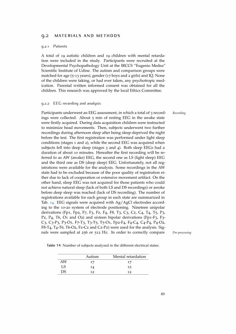
9.2 materials and methods
9.2.1 Patients
A total of 19 autistic children and 19 children with mental retarda-tion were included in the study. Participants were recruited at theDevelopmental Psychopathology Unit at the IRCCS “Eugenio Medea”Scientific Institute of Udine. The autism and comparison groups werematched for age (5-13 years), gender (17 boys and 2 girls) and IQ. Noneof the children were taking, or had ever taken, any psychotropic med-ication. Parental written informed consent was obtained for all thechildren. This research was approved by the local Ethics Committee.
9.2.2 EEG recording and analysis
Participants underwent an EEG assessment, in which a total of 3 record- Recording
ings were collected. About 5 min of resting EEG in the awake statewere firstly acquired. During data acquisition children were instructedto minimize head movements. Then, subjects underwent two furtherrecordings during afternoon sleep after being sleep-deprived the nightbefore the test. The first registration was performed under light sleepconditions (stages 1 and 2), while the second EEG was acquired whensubjects fell into deep sleep (stages 3 and 4). Both sleep EEGs had aduration of about 10 minutes. Hereafter the first recording will be re-ferred to as AW (awake) EEG, the second one as LS (light sleep) EEGand the third one as DS (deep sleep) EEG. Unfortunately, not all reg-istrations were available for the analysis. Some recordings in the AWstate had to be excluded because of the poor quality of registration ei-ther due to lack of cooperation or extensive movement artifact. On theother hand, sleep EEG was not acquired for those patients who couldnot achieve natural sleep (lack of both LS and DS recordings) or awokebefore deep sleep was reached (lack of DS recording). The number ofregistrations available for each group in each state are summarized inTab. 14. EEG signals were acquired with Ag/AgCl electrodes accord-ing to the 10-20 system of electrode positioning. Nineteen unipolarderivations (Fp1, Fp2, F7, F3, Fz, F4, F8, T3, C3, Cz, C4, T4, T5, P3,Pz, P4, T6, O1 and O2) and sixteen bipolar derivations (Fp1-F3, F3-C3, C3-P3, P3-O1, F7-T3, T3-T5, T5-O1, Fp2-F4, F4-C4, C4-P4, P4-O2,F8-T4, T4-T6, T6-O2, Fz-Cz and Cz-Pz) were used for the analysis. Sig-nals were sampled at 256 or 512 Hz. In order to correctly compare Pre-processing
Table 14: Number of subjects analyzed in the different electrical states.
Autism Mental retardationAW 17 17
LS 14 15
DS 12 12
89
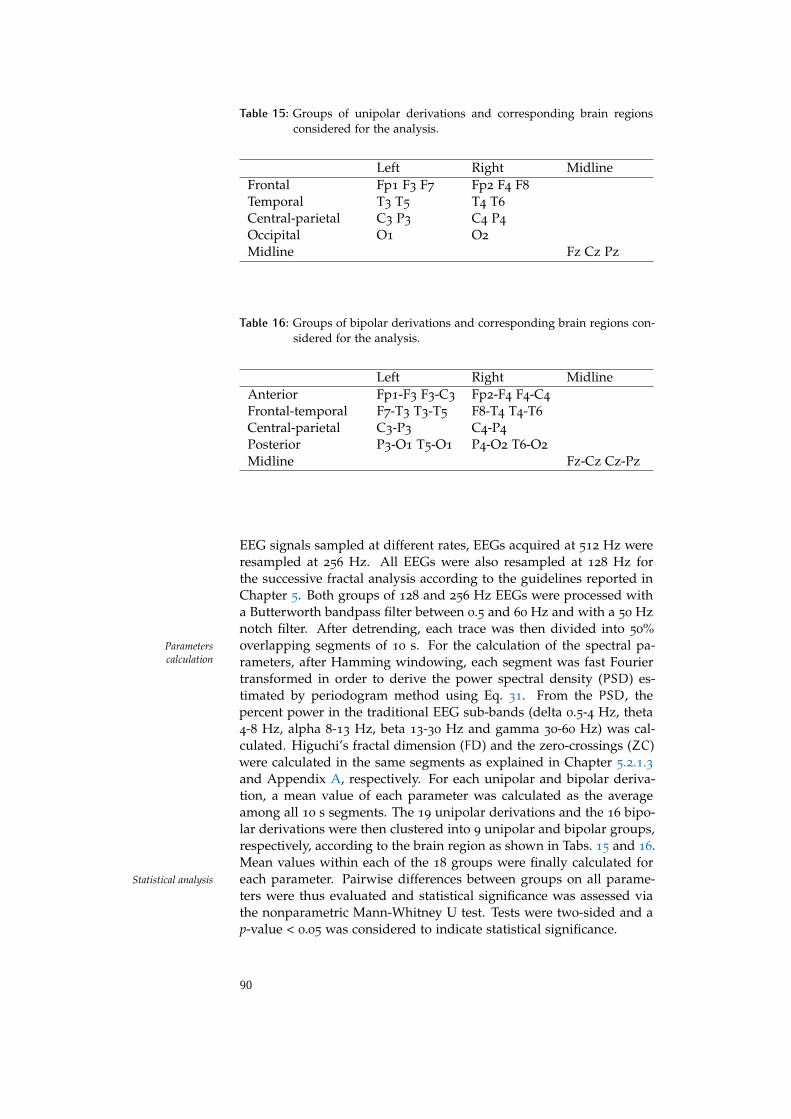
Table 15: Groups of unipolar derivations and corresponding brain regionsconsidered for the analysis.
Left Right MidlineFrontal Fp1 F3 F7 Fp2 F4 F8
Temporal T3 T5 T4 T6
Central-parietal C3 P3 C4 P4
Occipital O1 O2
Midline Fz Cz Pz
Table 16: Groups of bipolar derivations and corresponding brain regions con-sidered for the analysis.
Left Right MidlineAnterior Fp1-F3 F3-C3 Fp2-F4 F4-C4
Frontal-temporal F7-T3 T3-T5 F8-T4 T4-T6
Central-parietal C3-P3 C4-P4
Posterior P3-O1 T5-O1 P4-O2 T6-O2
Midline Fz-Cz Cz-Pz
EEG signals sampled at different rates, EEGs acquired at 512 Hz wereresampled at 256 Hz. All EEGs were also resampled at 128 Hz forthe successive fractal analysis according to the guidelines reported inChapter 5. Both groups of 128 and 256 Hz EEGs were processed witha Butterworth bandpass filter between 0.5 and 60 Hz and with a 50 Hznotch filter. After detrending, each trace was then divided into 50%overlapping segments of 10 s. For the calculation of the spectral pa-Parameters
calculation rameters, after Hamming windowing, each segment was fast Fouriertransformed in order to derive the power spectral density (PSD) es-timated by periodogram method using Eq. 31. From the PSD, thepercent power in the traditional EEG sub-bands (delta 0.5-4 Hz, theta4-8 Hz, alpha 8-13 Hz, beta 13-30 Hz and gamma 30-60 Hz) was cal-culated. Higuchi’s fractal dimension (FD) and the zero-crossings (ZC)were calculated in the same segments as explained in Chapter 5.2.1.3and Appendix A, respectively. For each unipolar and bipolar deriva-tion, a mean value of each parameter was calculated as the averageamong all 10 s segments. The 19 unipolar derivations and the 16 bipo-lar derivations were then clustered into 9 unipolar and bipolar groups,respectively, according to the brain region as shown in Tabs. 15 and 16.Mean values within each of the 18 groups were finally calculated foreach parameter. Pairwise differences between groups on all parame-Statistical analysis
ters were thus evaluated and statistical significance was assessed viathe nonparametric Mann-Whitney U test. Tests were two-sided and ap-value < 0.05 was considered to indicate statistical significance.
90
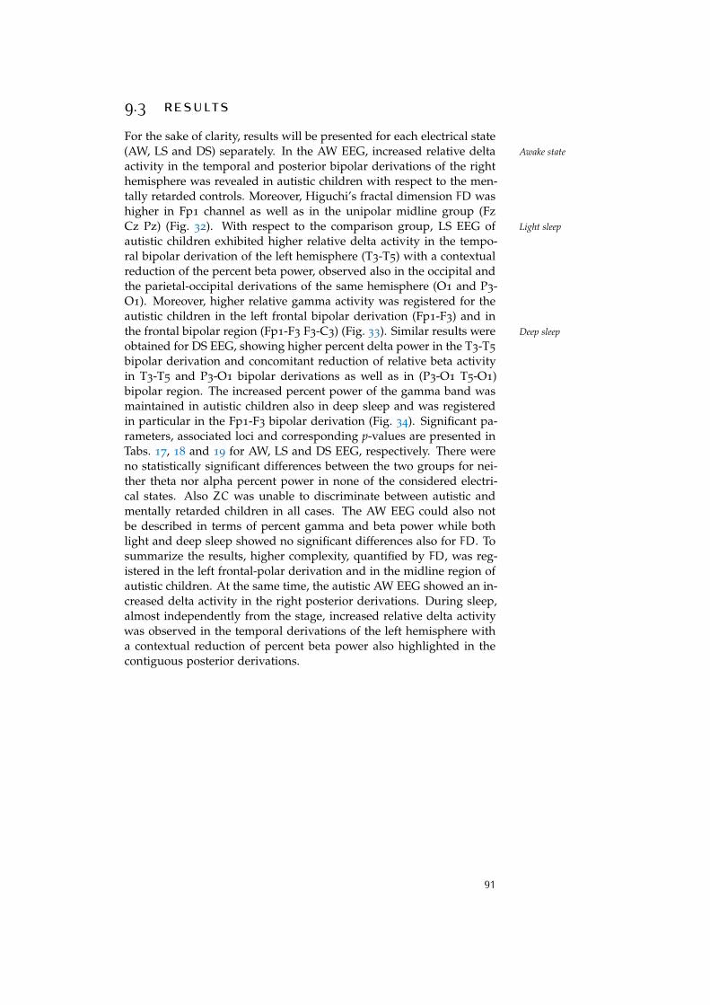
9.3 resultsFor the sake of clarity, results will be presented for each electrical state(AW, LS and DS) separately. In the AW EEG, increased relative delta Awake state
activity in the temporal and posterior bipolar derivations of the righthemisphere was revealed in autistic children with respect to the men-tally retarded controls. Moreover, Higuchi’s fractal dimension FD washigher in Fp1 channel as well as in the unipolar midline group (FzCz Pz) (Fig. 32). With respect to the comparison group, LS EEG of Light sleep
autistic children exhibited higher relative delta activity in the tempo-ral bipolar derivation of the left hemisphere (T3-T5) with a contextualreduction of the percent beta power, observed also in the occipital andthe parietal-occipital derivations of the same hemisphere (O1 and P3-O1). Moreover, higher relative gamma activity was registered for theautistic children in the left frontal bipolar derivation (Fp1-F3) and inthe frontal bipolar region (Fp1-F3 F3-C3) (Fig. 33). Similar results were Deep sleep
obtained for DS EEG, showing higher percent delta power in the T3-T5
bipolar derivation and concomitant reduction of relative beta activityin T3-T5 and P3-O1 bipolar derivations as well as in (P3-O1 T5-O1)bipolar region. The increased percent power of the gamma band wasmaintained in autistic children also in deep sleep and was registeredin particular in the Fp1-F3 bipolar derivation (Fig. 34). Significant pa-rameters, associated loci and corresponding p-values are presented inTabs. 17, 18 and 19 for AW, LS and DS EEG, respectively. There wereno statistically significant differences between the two groups for nei-ther theta nor alpha percent power in none of the considered electri-cal states. Also ZC was unable to discriminate between autistic andmentally retarded children in all cases. The AW EEG could also notbe described in terms of percent gamma and beta power while bothlight and deep sleep showed no significant differences also for FD. Tosummarize the results, higher complexity, quantified by FD, was reg-istered in the left frontal-polar derivation and in the midline region ofautistic children. At the same time, the autistic AW EEG showed an in-creased delta activity in the right posterior derivations. During sleep,almost independently from the stage, increased relative delta activitywas observed in the temporal derivations of the left hemisphere witha contextual reduction of percent beta power also highlighted in thecontiguous posterior derivations.
91
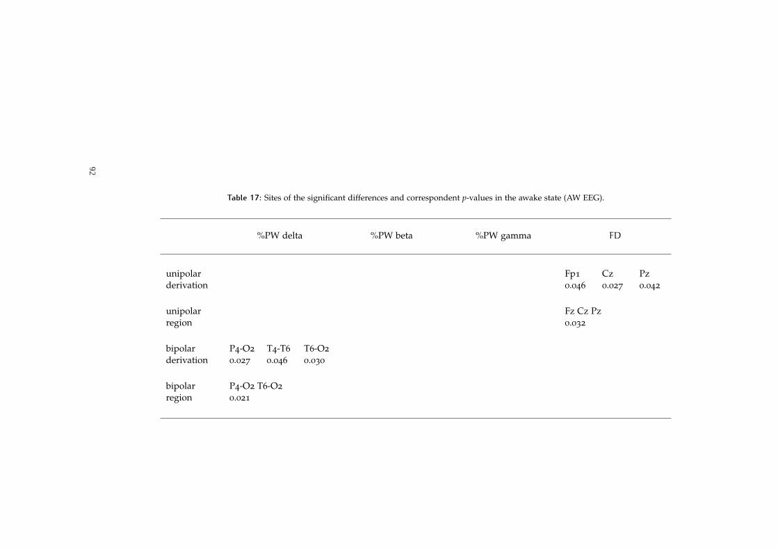
Table 17: Sites of the significant differences and correspondent p-values in the awake state (AW EEG).
%PW delta %PW beta %PW gamma FD
unipolar Fp1 Cz Pzderivation 0.046 0.027 0.042
unipolar Fz Cz Pzregion 0.032
bipolar P4-O2 T4-T6 T6-O2
derivation 0.027 0.046 0.030
bipolar P4-O2 T6-O2
region 0.021
92
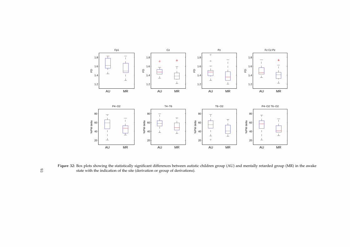
1.2
1.4
1.6
1.8
AU MRF
D
Fp1
1.2
1.4
1.6
1.8
AU MR
FD
Cz
1.2
1.4
1.6
1.8
AU MR
FD
Pz
1.2
1.4
1.6
1.8
AU MR
FD
Fz Cz Pz
20
40
60
80
AU MR
%P
W d
elta
P4−O2
20
40
60
80
AU MR%
PW
del
ta
T4−T6
20
40
60
80
AU MR
%P
W d
elta
T6−O2
20
40
60
80
AU MR
%P
W d
elta
P4−O2 T6−O2
Figure 32: Box plots showing the statistically significant differences between autistic children group (AU) and mentally retarded group (MR) in the awakestate with the indication of the site (derivation or group of derivations).
93
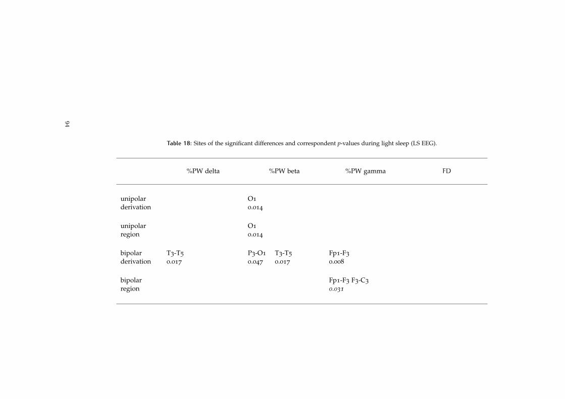
Table 18: Sites of the significant differences and correspondent p-values during light sleep (LS EEG).
%PW delta %PW beta %PW gamma FD
unipolar O1
derivation 0.014
unipolar O1
region 0.014
bipolar T3-T5 P3-O1 T3-T5 Fp1-F3
derivation 0.017 0.047 0.017 0.008
bipolar Fp1-F3 F3-C3
region 0.031
94

50
60
70
80
90
100
AU MR
%P
W d
elta
T3−T5
0
2
4
6
8
AU MR
%P
W g
amm
a
Fp1−F3
0
2
4
6
8
AU MR
%P
W g
amm
a
Fp1−F3 F3−C3
0
2
4
6
8
AU MR
%P
W b
eta
O1
0
2
4
6
8
AU MR
%P
W b
eta
P3−O1
0
2
4
6
8
AU MR
%P
W b
eta
T3−T5
Figure 33: Box plots showing the statistically significant differences between autistic children group (AU) and mentally retarded group (MR) during lightsleep with the indication of the site (derivation or group of derivations).
95

Table 19: Sites of the significant differences and correspondent p-values during deep sleep (DS EEG).
%PW delta %PW beta %PW gamma FD
unipolarderivation
unipolarregion
bipolar T3-T5 P3-O1 T3-T5 Fp1-F3
derivation 0.019 0.023 0.012 0.001
bipolar P3-O1 T5-O1
region 0.040
96

50
60
70
80
90
100
AU MR
%P
W d
elta
T3−T5
−1
0
1
2
3
AU MR
%P
W g
amm
a
Fp1−F3
0
1
2
3
4
5
6
AU MR
%P
W b
eta
P3−O1
0
1
2
3
4
5
6
AU MR
%P
W b
eta
T3−T5
0
1
2
3
4
5
6
AU MR
%P
W b
eta
P3−O1 T5−O1
Figure 34: Box plots showing the statistically significant differences between autistic children group (AU) and mentally retarded group (MR) during deepsleep with the indication of the site (derivation or group of derivations).
97
9.4 discussion
The study presented in this chapter is the first one in which the EEG ofautistic children is compared with that of mentally retarded subjects,matched for cognitive functioning, in the three major electrical states:awake state, light sleep and deep sleep. The relative power in the tradi-tional EEG sub-bands (delta, theta, alpha, beta and gamma), Higuchi’sfractal dimension and the zero-crossings were calculated and aver-aged for each unipolar/bipolar derivation and for each unipolar/bipo-lar group of derivations. Although available literature is very recentand limited, some preliminary studies on the comparison of autisticand normal EEG in the awake state have been published. Conflict-ing results, obtained with linear analysis, indicated increased gammapower [Grice et al., 2001], reduced theta activity in the anterior regionsof the brain [Chan et al., 2009] and higher power of the delta and thetaband in the frontal loci [Pop-Jordanova et al., 2010]. The fractal anal-ysis carried out by Ahmadlou et al. [2010] using Higuchi’s algorithmshowed significant differences in the frontal channels (F4, F7 and F8).Such results, difficult to interpret, have been presumptively correlatedto the cognitive, social and communication impairment, typical of neu-rological and developmental disorders.
The results achieved by the present investigation indicated higherirregularity of autistic awake EEG, quantified by Higuchi’s fractal di-mension, in the left frontal-polar channel (Fp1) and in the unipolarmidline group (Fz Cz Pz). This finding suggests that, for the sameIQ, the neuronal activity is more organized in autistic subjects thanin mentally retarded controls. As regards spectral analysis, the deltasub-band was the only one that provided percent power values dis-criminative in distinguishing among awake autistic and awake men-tally retarded EEG. Significant higher relative delta activity was foundaveraging the bipolar derivations in the right posterior region (P4-O2
T6-O2). This result becomes more interesting when associated to thoseachieved by sleep EEG analysis. Although nonlinear parameterizationdid not highlight significant differences, linear analysis revealed in-creased relative delta activity in T3-T5 derivation and a concomitantreduction of beta percent power in the left posterior bipolar region(P3-O1 T5-O1). In other words, a shift in slow activity from right toleft hemisphere was observed in the wake-to-sleep transition. Sucha result, deserving further investigation, is not of immediate under-standing. However, a possible explanation may concern informationprocessing and memory consolidation deficits, as well as abnormaltranscallosal transfer of information, which occur during sleep. Higherrelative gamma oscillations during light sleep were observed in autis-tic children with respect to mentally retarded controls in the left an-terior region of the brain. Since high frequency activity is related toperceptual and cognitive processes, partly impaired also in mental re-tardation, a higher percent power in the gamma sub-band may be anindicator for autistic perceptual and cognitive impairment.
98

9.5 conclusionThe study presented in this chapter was conducted with the aim ofcharacterizing the macro-structural organization of the EEG of autis-tic children with respect to that of mentally retarded controls. Frac-tal analysis suggests that the complexity of EEG signal in the awakestate is higher for autistic children with respect to controls, althoughsubjects were matched for cognitive functioning. Linear analysis re-vealed a posterior slow activity shift between awake and asleep statesfrom the right to the left hemisphere, which may be related to autis-tic deficits in information processing and memory consolidation, aswell as to abnormal transcallosal transfer of information. Moreover,higher relative gamma activity, associated with cognitive processes,was highlighted in autism. Future studies, to be performed on a largersample of recruited subjects including also normal children, shouldattempt to clarify and hopefully confirm these findings. QuantitativeEEG-based measures would be very important because early diagnosisallows early intervention with increased effectiveness.
99

10 C O N C L U S I O N
For the purpose of EEG nonlinear analysis, the possibility of fruit-fully exploring brain complexity directly in the time domain withoutthe need for phase space reconstruction would undoubtedly be advan-tageous.
After a review of the methods available in the literature for the anal-ysis of the fractal-like behavior of the EEG directly in the time domain,the Author selected and compared three widely used algorithms forthe estimation of the fractal dimension of waveforms. Higuchi’s algo-rithm outperformed box-counting and Katz’s methods, producing cor-rect estimates of the fractal dimension also on short traces, providedthat minimum sampling rate required to avoid aliasing is used. Theuse of the scaling relationship of fractional Brownian motion to obtainindirect estimates of the fractal dimension from the power-law expo-nent is, on the contrary, not recommended, since deviations from fBmwere observed by the Author. As long as a complete model of the EEGis lacking, direct estimation of the fractal dimension with Higuchi’salgorithms is preferable.
Higuchi’s fractal dimension was used to address three clinical is-sues: 1) the monitoring of carotid endarterectomy for the preventionof intraoperative stroke, 2) the assessment of the depth of anesthesiato monitor unconsciousness during surgery and 3) the analysis of themacro-structural organization of the EEG in autism with respect tomental retardation.
In the first study the fractal dimension was expected to reflect thepossible complexity drop due to hypoperfusion caused by artery clamp-ing. The efficacy of the parameter as a criterion to determine whethera shunt is indicated was evaluated on 140 surgical procedures. The pa-rameter did not achieve satisfactory results since the threshold selectedto minimize identification errors produced a sensitivity of barely 30%with 100% specificity. Higher thresholds improved sensitivity at the ex-pense of a fall in specificity. Both HFL linear index and ZC nonlinearparameter, on the contrary, obtained 100% overall accuracy resultingbetter indicators of cerebral suffering.
In the second investigation the fractal dimension was expected to re-flect the level of unconsciousness induced by the hypnotic agents dur-ing general anesthesia. The ability of the parameter to follow the depthof anesthesia from induction to recovery was assessed in 6 patients.Whereas the standalone parameter was not able to monitor too deepunconsciousness, characterized by burst suppression patterns, the frac-tal dimension compensated for burst suppression correctly quantifiedthe depth of anesthesia in all its phases.
101
In the discrimination of autism from mental retardation, the frac-tal dimension was significantly different in the anterior regions of thebrain and along the midline, while differences in some spectral pa-rameters were observed mainly in the posterior areas, suggesting thatlinear analysis and fractal analysis capture complimentary informationon brain functioning. The results of the fractal analysis, in particular,revealed that autistic children have more complex EEG sources withrespect to mentally retarded controls.
The results of the clinical studies suggest that, although linear spec-tral analysis still represents a valuable technique for the investigationof the EEG, time domain fractal analysis provides additional informa-tion on brain functioning which traditional analysis cannot achieve,making use of techniques of low computational cost. In conclusion,nonlinear processing of the EEG based on the analysis of the fractal-like behavior of the signal represents a powerful tool for the compre-hension of neuronal activity.
102
A A P P E N D I X
The zero-crossings (ZC) is a nonlinear parameter used in the analysisof random signals [Kedem, 1986]. It is computed by counting the num-ber of baseline crossings in a fixed time interval. Let x(1),x(2),...,x(N)
be a zero-mean stationary Gaussian time series. Consider the associ-ated clipped binary series y1(n) defined by:
y1(n) =
1, if x(n) > 0
0, if x(n) 6 0
(38)
with n = 1,2,...,N and let y2(n) be the associated series defined as:
y2(n) = y1(n+ 1) (39)
with n = 1, 2, ...,N− 1, where y2(N) = y2(N− 1). Three further binaryseries are defined by:
z1(n) = y1(n) OR y2(n)
z2(n) = y1(n) NAND y2(n)
z3(n) = z1(n) AND z2(n)
(40)
Then the ZC count is defined by the sum:
ZC =∑n
z3(n) (41)
Fruitful connections exist between ZC count and dominant frequency.When a certain frequency band becomes dominant, it attracts the nor-malized expected zero-crossings and ZC
2(N−1) admits values in thisband. Likewise, when a certain frequency f0 becomes significantlydominant then ZC
2(N−1) ' f0. In the extreme case when only f0 is
present, ZC2(N−1) = f0. This tendency of zero-crossings was called the
dominant frequency principle. As an example, consider the signal x(n):
x(n) = A cos(0.8n) +B cos(1.25n)
for n = 1,2,...,N with N = 200. ZC is a function of the weights A andB. When A = B = 1 there is no dominant frequency (Fig. 35). It resultsZC = 69 and πZC
199 = 1.095 which is in the range 0.8-1.25 as expected.When A = 0.8 and B = 1, the frequency 1.25 is dominant (Fig. 35).It results ZC = 79 and πZC
199 = 1.247 which is very close to 1.25 inagreement with the dominant frequency principle.
103
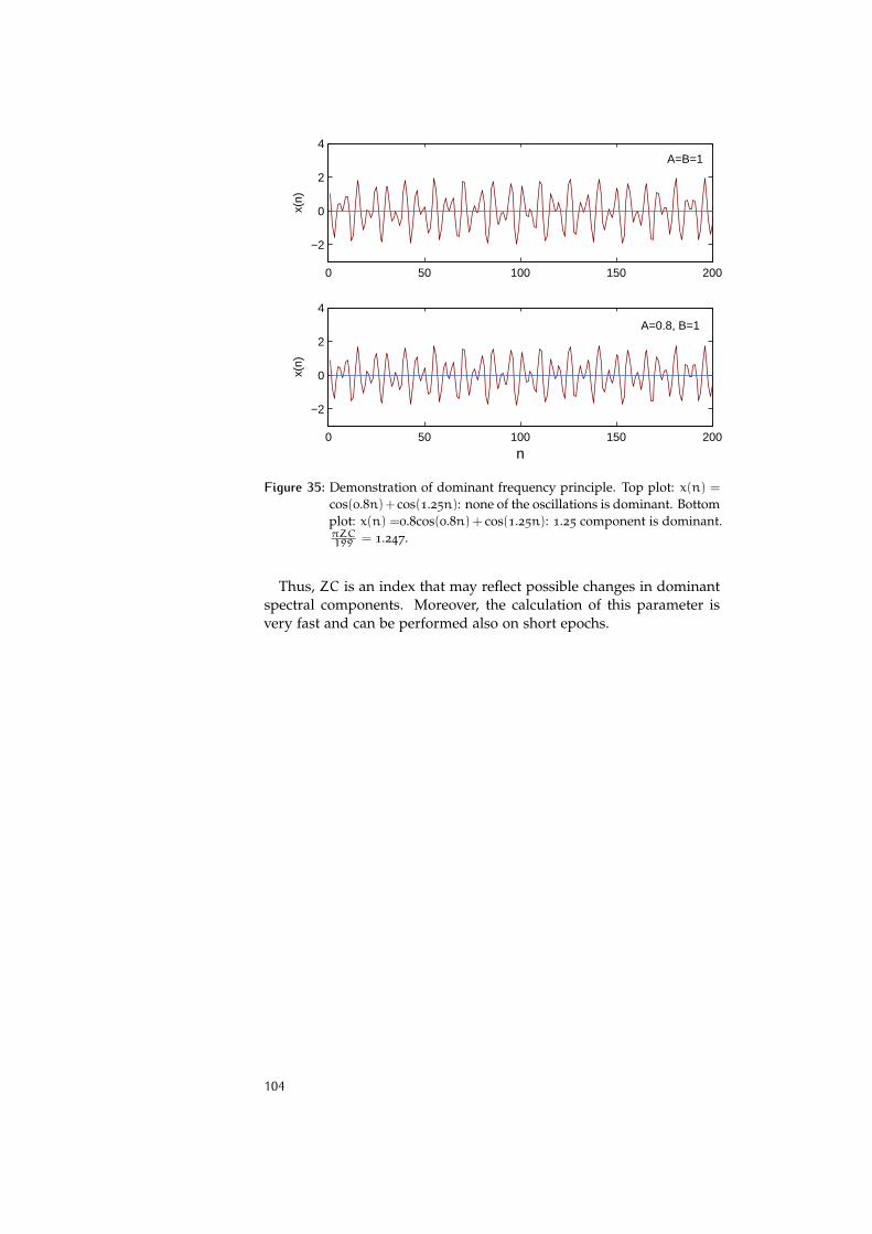
0 50 100 150 200
−2
0
2
4
x(n)
0 50 100 150 200
−2
0
2
4
n
x(n)
A=B=1
A=0.8, B=1
Figure 35: Demonstration of dominant frequency principle. Top plot: x(n) =cos(0.8n)+ cos(1.25n): none of the oscillations is dominant. Bottomplot: x(n) =0.8cos(0.8n) + cos(1.25n): 1.25 component is dominant.πZC199 = 1.247.
Thus, ZC is an index that may reflect possible changes in dominantspectral components. Moreover, the calculation of this parameter isvery fast and can be performed also on short epochs.
104
B I B L I O G R A P H Y
Abry, P and F Sellan [1996], “The wavelet-based synthesis for fractionalBrownian motion proposed by F. Sellan and Y. Meyer: remarks andfast implementation,” Appl and Comput Harm Anal, 3, 4, pp. 377–383.(Cited on p. 39.)
Accardo, A, M Affinito, M Carrozzi, and F Bouquet [1997], “Use ofthe fractal dimension for analysis of electroencephalographic timeseries,” Biol Cybern, 77, 5, pp. 339–350. (Cited on pp. 34, 36, 48.)
Acharya, UR, O Faust, N Kannathal, T Chua, and S Laxminarayan[2005], “Non-linear analysis of EEG signals at vaious sleep stages,”Comput Methods Programs Biomed, 80, pp. 37–45. (Cited on p. 34.)
Ahmadlou, M, H Adeli, and A Adeli [2010], “Fractality and wavelet-chaos-neural network for EEG-based diagnosis of autistic spectrumdisorder,” J Clin Neurophysiol, 27, 5, pp. 328–333. (Cited on pp. 34, 88,98.)
– [2011], “Fractality and wavelet-chaos-methodology for EEG-baseddiagnosis of Alzheimer disease,” Alzheimer Dis Assoc Disord, 25, 1,pp. 85–92. (Cited on p. 34.)
Bassingthwaighte, JB, LS Liebovitch, and BJ West [1994], Fractal physi-ology, Oxford University Press, New York. (Cited on pp. 26, 51.)
Belmonte, MK, G Allen, A Beckel-Mitchener, LM Boulanger, RA Carper,and SJ Webb [2004], “Autism and abnormal development of brainconnectivity,” J Neurosci, 24, 42, pp. 9228–9231. (Cited on p. 87.)
Berry, MV [1979], “Diffractals,” J Phys A, 12, pp. 781–797. (Cited onp. 53.)
Berry, MV and ZV Lewis [1980], “On the Weierstrass-Mandelbrot frac-tal function,” Proc R Soc Lond, 370, 1743, pp. 459–484. (Cited on p. 38.)
Blume, WT, GG Ferguson, and DK McNeill [1986], “Significance ofEEG changes at carotid endarterectomy,” Stroke, 17, pp. 891–897.(Cited on p. 71.)
Bojic, T, A Vuckovic, and A Kalauzi [2010], “Modeling EEG fractaldimension changes in wake and drowsy states in humans - a prelim-inary study,” J Theor Biol, 262, 2, pp. 214–222. (Cited on p. 34.)
Bonebakker, AE, M Jelicic, J Passchier, and B Bonke [1996], “Memoryduring general anesthesia: practical and methodological aspects,”Conscious Cogn, 5, 4, pp. 542–561.
Bosl, W, A Tierney, H Tager-Flusberg, and C Nelson [2011], “EEG com-plexity as a biomarker for autism spectrum disorder risk,” BMC Med,9, p. 18. (Cited on p. 34.)
Bruhn, J, TW Bouillon, and SL Shafer [2000], “Bispectral index (BIS)and burst suppression: revealing a part of the BIS algorithm.,” J ClinMonit Comput, 16, 8, pp. 593–596. (Cited on pp. 79, 80.)
Buckley, AW, AJ Rodriguez, K Jennison, J Buckley, A Thurm, S Sato,and S Swedo [2010], “Rapid eye movement sleep percentage in chil-dren with autism compared with children with developmental delay
105
and typical development,” Arch Pediatr Adolesc Med, 164, 11, pp. 1032–1037. (Cited on p. 88.)
Carrozzi, M, A Accardo, and F Bouquet [2004], “Analysis of sleep-stage characteristics in full-term newborns by means of spectral andfractal parameters,” Sleep, 27, 7, pp. 1384–1393. (Cited on pp. 34, 40,71.)
Catarino, A, O Churches, S Baron-Cohen, A Andrade, and Ring H[2011], “Atypical EEG complexity in autism spectrum conditions: amultiscale entropy analysis,” Clin Neurophysiol, 122, 12, pp. 2375–2383. (Cited on pp. 34, 88.)
Chan, AS, MC Cheung, YM Han, SL Sze, WW Leung, HS Man, andCY To [2009], “Executive function deficits and neural discordance inchildren with Autism Spectrum Disorders,” Clin Neurophysiol, 120, 6,pp. 1107–1115. (Cited on pp. 88, 98.)
Chouvarda, I, MO Mendez, V Rosso, AM Bianchi, L Parrino, A Grassi,M Terzano, N Maglaveras, and S Cerutti [2011], “Predicting EEGcomplexity from sleep macro and microstructure,” Physiol Meas, 32,8, pp. 1083–1101. (Cited on p. 34.)
Cursi, M, MV Meraviglia, GF Fanelli, R Chiesa, A Tirelli, G Comi, andF Minicucci [2005], “Electroencephalographic background desynchro-nization during cerebral blood flow reduction,” Clin Neurophysiol,116, 11, pp. 2577–2585. (Cited on pp. 62, 64, 70, 71, 73.)
Daneshyari, M, LL Kamkar, and M Daneshyari [2010], “Epileptic EEG:a comprehensive study of nonlinear behavior,” Adv Exp Med Biol,680, pp. 677–683. (Cited on p. 34.)
Doyle, PW and BF Matta [1999], “Burst suppression or isoelectric en-cephalogram for cerebral protection: evidence from metabolic sup-pression studies,” Br J Anaesth, 83, 4, pp. 580–584. (Cited on p. 78.)
Drover, DR, HJ Lemmens, ET Pierce, G Plourde, G Loyd, E Ornstein,LS Prichep, RJ Chabot, and L Gugino [2002], “Patient State Index:titration of delivery and recovery from propofol, alfentanil, and ni-trous oxide anesthesia,” Anesthesiology, 97, 1, pp. 82–89. (Cited onp. 76.)
Errando, CL, JC Sigl, M Robles, E Calabuig, J García, F Arocas, RHigueras, E Del Rosario, D López, CM Peiró, JL Soriano, S Chaves,F Gil, and R García-Aguado [2008], “Awareness with recall duringgeneral anaesthesia: a prospective observational evaluation of 4001
patients,” Br J Anaesth, 101, 2, pp. 178–185. (Cited on p. 76.)Esteller, R, G Vachtsevanos, J Echauz, and B Litt [2001], “A comparison
of waveform fractal dimension algorithms,” IEEE Trans Biomed Eng,48, 2, pp. 177–183. (Cited on pp. 34, 35, 48.)
Ferenets, R, T Lipping, A Anier, V Jäntti, S Melto, and S Hovilehto[2006], “Comparison of entropy and complexity measures for the as-sessment of depth of sedation,” IEEE Trans Biomed Eng, 53, 6, pp. 1067–1077. (Cited on p. 34.)
Ferenets, R, A Vanluchene, T Lipping, B Heyse, and MM Struys [2007],“Behavior of entropy/complexity measures of the electroencephalo-gram during propofol-induced sedation: dose-dependent effects of
106
remifentanil,” Anesthesiology, 106, 4, pp. 696–706. (Cited on pp. 34,76.)
Fraser, AM and HL Swinney [1986], “Independent coordinates for strangeattractors from mutual information,” Phys Rev A, 33, 2, pp. 1134–1140. (Cited on p. 19.)
Ghali, R, EG Palazzo, DI Rodriguez, M Zammit, DL Loudenback, RPDeMuth, MP Spencer, and LR Sauvage [1997], “Transcranial dopplerintraoperative monitoring during carotid endarterectomy: experiencewith regional or general anesthesia, with and without shunting,”Ann Vasc Surg, 11, 1, pp. 9–13. (Cited on p. 61.)
Grassberger, P and I Procaccia [1983], “Measuring the strangeness ofstrange attractors,” Physica D, 9, 1-2, pp. 189–208. (Cited on p. 16.)
Grice, SJ, MW Spratling, A Karmiloff-Smith, H Halit, G Csibra, M deHaan, and MH Johnson [2001], “Disordered visual processing andoscillatory brain activity in autism and Williams syndrome,” Neu-roreport, 12, 12, pp. 2697–2700. (Cited on pp. 88, 98.)
Henderson, G, E Ifeachor, N Hudson, C Goh, N Outram, S Wimalaratna,C Del Percio, and F Vecchio [2006], “Development and assessment ofmethods for detecting dementia using the human electroencephalo-gram,” IEEE Trans Biomed Eng, 53, 8, pp. 1557–1568. (Cited on p. 71.)
Hénon, M [1976], “A two-dimensional mapping with a strange attrac-tor,” Commun Math Phys, 50, 1, pp. 69–77. (Cited on p. 15.)
Henry, B, N Lovell, and F Camacho [2001], “Nonlinear dynamics timeseries analysis,” in Nonlinear biomedical signal processing, vol. II, MetinAkay, New York. (Cited on p. 14.)
Higuchi, T [1988], “Approach to an irregular time series on the basisof the fractal theory,” Physica D, 31, 2, pp. 277–283. (Cited on pp. 30,33–35, 37, 53.)
– [1990], “Relationship between the fractal dimension and the powerlaw index for a time series: A numerical investigation,” Physica D,46, pp. 254–264. (Cited on pp. 51, 55.)
Hobson, JA and EF Pace-Schott [2002], “The cognitive neuroscienceof sleep: neuronal systems, consciousness and learning,” Nat RevNeurosci, 3, 9, pp. 679–693. (Cited on p. 88.)
Inouye, T, S Ukai, K Shinosaki, A Iyama, Y Matsumoto, and S Toi[1994], “Changes in the fractal dimension of alpha envelope fromwakefulness to drowsiness in the human electroencephalogram,” Neu-rosci Lett, 174, 1, pp. 105–108. (Cited on p. 34.)
Jasper, H [1958], “Report of the Committee on Methods of Clinical Ex-amination in Electroencephalography: 1957,” Electroencephalogr ClinNeurophysiol, 10, pp. 370–375. (Cited on p. 10.)
Jones, JG [1994], “Perception and memory during general anesthesia,”Br J Anaesth, 73, 1, pp. 31–37. (Cited on p. 75.)
Jordan, D, G Schneider, A Hock, T Hensel, G Stockmanns, and EFKochs [2006], “EEG parameters and their combination as indicatorsof depth of anaesthesia,” Biomed Tech Berlin, 51, 2, pp. 89–94. (Citedon p. 76.)
Kalkman, CJ [2004], “Con: Routine shunting is not the optimal manage-ment of the patient undergoing carotid endarterectomy, but neither
107
is neuromonitoring,” J Cardiothorac Vasc Anesth, 18, 3, pp. 381–383.(Cited on p. 61.)
Kantz, H and T Schreiber [2004], Nonlinear time series analysis, SecondEdition, Cambridge University Press, New York, chap. 1-6. (Cited onp. 14.)
Katz, M [1988], “Fractals and the analysis of waveforms,” Comput BiolMed, 18, 3, pp. 145–156. (Cited on pp. 30, 33–36.)
Kedem, B [1986], “Spectral analysis and discrimination by zero-crossings,”in vol. 74, 11, pp. 1477–1493. (Cited on pp. 64, 80, 103.)
Kelley, SD [2010], Monitoring consciousness using the Bispectral Index(BISTM) during anesthesia: a pocket guide for clinicians. (Cited on p. 76.)
Kennel, MB, R Brown, and HD Abarbanel [1992], “Determining em-bedding dimension for phase-space reconstruction using a geomet-rical construction,” Phys Rev A, 45, 6, pp. 3403–3411. (Cited on p. 18.)
Klimesch, W [1999], “EEG alpha and theta oscillations reflect cognitiveand memory performance: a review and analysis,” Brain ResearchReview, 29, 2-3, pp. 169–195.
Klockars, J, A Hiller, S Münte, MJ van Gils, and T Taivainen [2011],“Spectral Entropy as a Measure of Hypnosis and Hypnotic DrugEffect of Total Intravenous Anesthesia in Children during Slow In-duction and Maintenance,” Anesthesiology. (Cited on p. 76.)
Kreuer, S, A Biedler, R Larsen, S Altmann, and W Wilhelm [2003],“Narcotrend monitoring allows faster emergence and a reduction ofdrug consumption in propofol-remifentanil anesthesia,” Anesthesiol-ogy, 99, 1, pp. 34–41. (Cited on p. 76.)
Kulisek, R, Z Hrncir, M Hrdlicka, L Faladova, K Sterbova, P Krsek, EVymlatilova, M Palus, A Zumrová, and V Komárek [2008], “Nonlin-ear analysis of the sleep EEG in children with pervasive develop-mental disorder,” Neuro Endocrinol Lett, 29, 4, pp. 512–517. (Cited onp. 88.)
Laman, DM, CS van der Reijden, GH Wieneke, H van Duijn, and ACvan Huffelen [2012], “EEG evidence for shunt requirement duringcarotid endarterectomy: optimal EEG derivations with respect tofrequency bands and anesthetic regimen,” J Clin Neurophysiol, 18, 4,pp. 353–363. (Cited on pp. 63, 71.)
Li, D, X Li, S Hagihira, and JW Sleigh [2011], “The effect of isoflu-rane anesthesia on the electroencephalogram assessed by harmonicwavelet bicoherence-based indices,” J Neural Eng, 8, 5. (Cited onp. 76.)
Liang, Z, D Li, G Ouyang, Y Wang, LJ Voss, JW Sleigh, and X Li [2011],“Clin Neurophysiol,” Multiscale rescaled range analysis of EEG record-ings in sevoflurane anesthesia. (Cited on p. 76.)
Lin, DC, A Sharif, and HC Kwan [2006], “Scaling and organizationof electroencephalographic background activity and alpha rhythmin healthy young adults,” Biol Cybern, 95, 5, pp. 401–411. (Cited onp. 71.)
Lorenz, EN [1963], “Deterministic nonperiodic flow,” J Atmos Sci, 20,2, pp. 130–141. (Cited on p. 15.)
108

Malow, BA [2004], “Sleep disorders, epilepsy, and autism,” Ment RetardDev Disabil Res Rev, 10, 2, pp. 122–125. (Cited on p. 88.)
Mandelbrot, BB [1982], The fractal geometry of nature, Freeman, NewYork. (Cited on pp. 30, 33–35.)
– [1985], “Self-affine fractals and fractal dimension,” Phys Scr, 32, 4,pp. 257–260. (Cited on p. 33.)
Mandelbrot, BB and JW Van Ness [1968], “Fractional Brownian mo-tions: Fractional noises and applications,” SIAM Rev, 10, 4, pp. 422–437. (Cited on pp. 25, 53.)
Maquet, P [2001], “The role of sleep in learning and memory,” Science,294, 5544, pp. 1048–1052. (Cited on p. 88.)
Maragos, P and FK Sun [1983], “Measuring the fractal dimension ofsignals: morphological covers and iterative optimization,” IEEE TransSignal Proc, 41, 1, pp. 108–121. (Cited on p. 30.)
McFarland, HR, JA Jr Pinkerton, and D Frye [1988], “Continuous elec-troencephalographic monitoring during carotid endarterectomy,” JCardiovasc Surg, 29, 1, pp. 12–18. (Cited on p. 61.)
Mengotti, P, S D’Agostini, R Terlevic, C De Colle, E Biasizzo, D Lon-dero, A Ferro, G Rambaldelli, M Balestrieri, S Zanini, F Fabbro, MMolteni, and P Brambilla [2011], “Altered white matter integrityand development in children with autism: a combined voxel-basedmorphometry and diffusion imaging study,” Brain Res Bull, 84, 2,pp. 189–195. (Cited on p. 87.)
Miller, A, JW Sleigh, J Barnard, and DA Steyn-Ross [2004], “Does bis-pectral analysis of the electroencephalogram add anything but com-plexity?” Br J Anaesth, 92, 1, pp. 8–13. (Cited on p. 76.)
Miller, RD [2005], Miller’s anesthesia, 6th ed., Elsevier Churchill Living-stone, Philadelphia. (Cited on p. 76.)
Minicucci, F, M Cursi, C Fornara, C Rizzo, R Chiesa, A Tirelli, G Fanelli,MV Meraviglia, L Giacomotti, and G Comi [2000], “Computer-assistedEEG monitoring during carotid endarterectomy,” J Clin Neurophysiol,17, 1, pp. 101–107. (Cited on pp. 62, 65, 71.)
Mizuno, T, T Takahashi, RY Cho, M Kikuchi, T Murata, K Takahashi,and Y Wada [2010], “Assessment of EEG dynamical complexity inAlzheimer’s disease using multiscale entropy,” Clin Neurophysiol, 121,9, pp. 1438–1446. (Cited on p. 34.)
Moore, WS, JM Yee, and AD Hall [1973], “Collateral cerebral bloodpressure - An index of tolerance to temporary carotid occlusion,”AMA Arch Surg, 106, 4, pp. 520–523. (Cited on p. 61.)
Morimoto, Y, S Hagihira, Y Koizumi, K Ishida, M Matsumoto, andT Sakabe [2004], “The relationship between bispectral index andelectroencephalographic parameters during isoflurane anesthesia,”Anesth Analg, 98, 5, pp. 1336–1340. (Cited on p. 76.)
Osterman, JE, J Hopper, WJ Heran, TM Keane, and BA van der Kolk[2001], “Awareness under anesthesia and the development of post-traumatic stress disorder,” Gen Hosp Psychiatry, 23, 4, pp. 198–204.(Cited on p. 75.)
109
Packard, NH, JP Crutchfield, JD Farmer, and RS Shaw [1980], “Geom-etry from a time series,” Phys Rev Lett, 45, 9, pp. 712–716. (Cited onp. 18.)
Paramanathan, P and R Uthayakumar [2008], “Application of fractaltheory in analysis of human electroencephalographic signals,” Com-put Biol Med, 38, 3, pp. 372–378. (Cited on pp. 30, 34, 35, 48.)
Peitgen, HO and D Saupe [1988], The science of fractal images, Springer-Verlag, New York. (Cited on p. 21.)
Penn, AI and MH Loew [1997], “Estimating fractal dimension withfractal interpolation function models,” IEEE Trans Med Imaging, 16,6, pp. 930–937. (Cited on p. 55.)
Penn, HE [2006], “Neurobiological correlates of autism: a review ofrecent research,” Child Neuropsychol, 12, 1, pp. 57–59. (Cited on p. 87.)
Petrosian, A [1995], “Kolmogorov complexity of finite sequences andrecognition of different preictal EEG patterns,” Proc IEEE Symp Comp-uter-Based Medical Syst. (Cited on pp. 30, 34.)
Philip, RC, MR Dauvermann, HC Whalley, K Baynham, SM Lawrie,and AC Stanfield [2012], “A systematic review and meta-analysisof the fMRI investigation of autism spectrum disorders,” NeurosciBiobehav Rev, 36, 2, pp. 901–942. (Cited on p. 87.)
Phothisonothai, M and M Nakagawa [2009], “A classification methodof different motor imagery tasks based on fractal features for brain-machine interface,” J Integr Neurosci, 8, 1, pp. 95–122. (Cited on pp. 34,52.)
Pinkerton, JA Jr [2002], “EEG as a criterion for shunt need in carotidendarterectomy,” Ann Vasc Surg, 16, 6, pp. 756–761. (Cited on p. 61.)
Plestis, KA, P Loubser, EM Mizrahi, G Kantis, ZD Jiang, and JF How-ell [1997], “Continuous electroencephalographic monitoring and se-lective shunting reduces neurologic morbidity rates in carotid en-darterectomy,” J Vasc Surg, 25, 4, pp. 620–628. (Cited on p. 61.)
Polychronaki, GE, PY Ktonas, S Gatzonis, A Siatouni, PA Asvestas,H Tsekou, D Sakas, and KS Nikita [2010], “Comparison of fractal di-mension estimation algorithms for epileptic seizure onset detection,”J Neural Eng, 4, p. 046007. (Cited on p. 34.)
Pop-Jordanova, N, T Zorcec, A Demerdzieva, and Z Gucev [2010],“QEEG characteristics and spectrum weighted frequency for chil-dren diagnosed as autistic spectrum disorder,” Nonlinear Biomed Phys,4, 1. (Cited on pp. 88, 98.)
Pritchard, WS [1992], “The brain in fractal time: 1/f-like power spec-trum scaling of the human electroencephalogram,” Intern J Neuro-science, 66, pp. 119–129. (Cited on pp. 25, 29, 30, 52.)
Raghavendra, BS and DN Dutt [2009], “A note on fractal dimensionsof biomedical waveforms,” Comput Biol Med, 39, 11, pp. 1006–1012.(Cited on pp. 34, 38, 39, 48.)
Raghavendra, BS, DN Dutt, HN Halahalli, and JP John [2009], “Com-plexity analysis of EEG in patients with schizophrenia using fractaldimension,” Physiol Meas, 30, 8, pp. 795–808. (Cited on p. 34.)
Rampil, IJ [1998], “A primer for EEG signal processing in anesthesia,”Anesthesiology, 89, 4, pp. 981–1001. (Cited on p. 80.)
110
Ramsay, MA, TM Savege, BR Simpson, and R Goodwin [2012], “Con-trolled sedation with alphaxalone-alphadolone,” Br Med J, 2, 5920,pp. 656–659. (Cited on p. 76.)
Rankine, L, N Stevenson, M Mesbah, and B Boashash [2007], “A non-stationary model of newborn EEG,” IEEE Trans Biomed Eng, 54, 1,pp. 19–28. (Cited on pp. 34, 52.)
Rapin, I [1997], “Autism,” N Engl J Med, 337, 2, pp. 97–104. (Cited onp. 87.)
Rippon, G, J Brock, C Brown, and J Boucher [2007], “Disordered con-nectivity in the autistic brain: challenges for the "new psychophysi-ology",” Int J Psychopshysiol, 63, 2, pp. 164–172. (Cited on p. 87.)
Salvian, AJ, DC Taylor, YN Hsiang, HD Hildebrand, HK Litherland,MF Humer, PA Teal, and DB MacDonald [2012], “Selective shuntwith EEG monitoring is safer than routine shunting for carotid en-darterectomy,” Cardiovasc Surg, 5, 5, pp. 481–485. (Cited on pp. 61,71, 73.)
Sanei, S and J Chambers [2007], EEG signal processing, Wiley, Chichester,England, chap. 1. (Cited on p. 7.)
Sauer, T, J Yorke, and M Casdagli [1994], “Embedology,” J Stat Phys,65, 3-4, pp. 579–616. (Cited on p. 18.)
Schneider, G, S Schöniger, and E Kochs [2004], “Does bispectral analy-sis add anything but complexity? BIS sub-components may be supe-rior to BIS for detection of awareness,” Br J Anaesth, 93, 4, pp. 596–597. (Cited on p. 76.)
Schreiber, T [1997], “Detecting and analyzing nonstationarity in a timeseries using nonlinear cross predictions,” Phys Rev Lett, 78, 5, pp. 843–846. (Cited on pp. 40, 53.)
Schweiger, H, HD Kamp, and M Dinkel [1991], “Somatosensory-evokedpotentials during carotid artery surgery: experience in 400 opera-tions,” Surgery, 109, 5, pp. 602–609. (Cited on p. 61.)
Schwender, D, H Kunze-Kronawitter, P Dietrich, S Klasing, H Forst,and C Madler [1998], “Conscious awareness during general anaes-thesia: patientsí perceptions, emotions, cognition and reactions,” BrJ Anaesth, 80, 2, pp. 133–139. (Cited on p. 75.)
Sevcik, C [2006], “On fractal dimension of waveforms,” Chaos SolitonFract, 28, pp. 579–580. (Cited on p. 30.)
Shah, DM, RC 3rd Darling, BB Chang, DE Bock, PS Paty, and RPLeather [1994], “Carotid endarterectomy in awake patients: its safety,acceptability, and outcome,” J Vasc Surg, 19, 6, pp. 1015–1019. (Citedon p. 61.)
Sleigh, JW, DA Steyn-Ross, ML Steyn-Ross, ML Williams, and P Smith[2001], “Comparison of changes in electroencephalographic measuresduring induction of general anaesthesia: influence of the gamma fre-quency band and electromyogram signal,” Br J Anaesth, 86, 1, pp. 50–58. (Cited on pp. 78, 84.)
Takagi, T [1903], “A simple example of a continuous function withoutderivative,” Proc Phys Math Japan, 1, pp. 176–177. (Cited on p. 39.)
111
Takens, F [1981], “Detecting strange attractors in turbulence,” in Dy-namical systems and turbulence, ed. by DA Rand and LS Young, Berlin.(Cited on p. 18.)
Tuchman, R, M Alessandri, and M Cuccaro [2010], “Autism spectrumdisorders and epilepsy: moving towards a comprehensive approachto treatment,” Brain Dev, 32, 9, pp. 19–30. (Cited on p. 88.)
Van Putten, MJ [2006], “Extended BSI for continuous EEG monitoringin carotid endarterectomy,” Clin Neurophysiol, 117, 12, pp. 2661–2666.(Cited on pp. 62, 64–66, 70, 72.)
Van Putten, MJ, JM Peters, SM Mulder, JA de Haas, CM Bruijninckx,and DL Tavy [2004], “A brain symmetry index (BSI) for online EEGmonitoring in carotid endarterectomy,” Clin Neurosphysiol, 115, 5,pp. 1189–1194. (Cited on pp. 62, 64, 70, 72.)
Viertiö-Oja, H, V Maja, M Särkelä, P Talja, N Tenkanen, H Tolvanen-Laakso, M Paloheimo, A Vakkuri, A Yli-Hankala, and P Meriläinen[2004], “Description of the EntropyTM algorithm as applied in theDatex-Ohmeda S/5
TM Entropy Module,” Acta Anaesthesiol Scand, 48,2, pp. 154–161. (Cited on p. 76.)
Visser, GH, GH Wieneke, and AC van Huffelen [1999], “Carotid en-darterectomy monitoring: patterns of spectral EEG changes due tocarotid artery clamping,” Clin Neurophysiol, 110, 2, pp. 286–294. (Citedon pp. 61, 65, 73.)
Visser, GH, GH Wieneke, AC Van Huffelen, JW De Vries, and PFBakker [2001], “The development of spectral EEG changes duringshort periods of circulatory arrest,” J Clin Neurophysiol, 18, 2, pp. 169–177. (Cited on p. 62.)
Von Koch, H [1904], “Sur une courbe continue sans tangente, obtenuepar une construction géométrique élémentaire,” Arkiv mat astron fys,1, pp. 681–704. (Cited on p. 22.)
Wilson, TW, DC Rojas, ML Reite, PD Teale, and SJ Rogers [2007], “Chil-dren and adolescents with autism exhibit reduced MEG steady-stategamma responses,” Biol Psychiatry, 62, 3, pp. 192–197. (Cited onp. 87.)
112

L I S T O F P U B L I C AT I O N S
This thesis is based on the following original publications:
1. Accardo, A, M Cusenza and F Monti [2009], “Linear and non-linearparameterization of EEG during monitoring of carotid endarterec-tomy,” Comput Biol Med, 39, 6, pp. 512-518.
2. Cusenza, M and A Accardo [2010], “Estimation of EEG fractal di-mension: sensitivity to sampling frequency and time window length,”Atti del Secondo Congresso Nazionale di Bioingegneria (GNB 2010), pp.463-464.
3. Cusenza, M and A Accardo [2010], “Self-affinity in brain activity: re-lationship between fractal dimension and power-law beta exponentof EEG in sleeping newborns,” ESBME Proc.
4. Cusenza, M and A Accardo [2012], “Sensitivity to sampling fre-quency and time window length in the estimation of EEG fractaldimension,” submitted to Biological Cybernetics, manuscript numberBICY-D-12-00026.
5. Cusenza, M, A Accardo and A Orsini [2012], “EEG fractal dimen-sion combined with burst suppression ratio as a measure of depthof anesthesia,” accepted for 2012 World Congress on Medical Physicsand Biomedical Engineering (WC 2012), paper ID A11011.
6. Cusenza, M, A Accardo, S Zanini and P Brambilla [2012], “Charac-terization of awake and sleep EEG in autistic children,” submittedto Terzo Congresso Nazionale di Bioingegneria (GNB 2012).
Supplementary publications related to the fractal analysis of the EEGbut not included in this thesis:
7. Cusenza, M, A Accardo, F Monti and P Bramanti [2010], “Linearand non-linear effects of gradient artifact filtering methods in si-multaneous EEG-fMRI,” Biomed Sci Instrum, 46, pp. 374-379.
Other publications related to the fractal analysis of the heart rate vari-ability, not included in this thesis:
8. Cusenza, M, A Accardo, G D’Addio and G Corbi [2010], “Relation-ship between fractal dimension and power-law exponent of heartrate variability in normal and heart failure subjects,” Computers inCardiology Proc, 37, pp. 935-938.
9. Cusenza, M, A Accardo and G D’Addio [2011], “Day-time andnight-time HRV ultradian rhythms in normal and pathological sub-jects,” IFMBE Proc, 37, pp. 450-453.
113

10. Accardo, A, M Cusenza, A De Felice and G D’Addio [2012], “Ul-tradian rhytms during day and night in normal and COPD sub-jects,” submitted to XXIV European Medical Informatics Conference(MIE 2012).
114
I N D E X
10-20 system, 10
attractor, 15
strange attractor, 15
autism, 87
awareness, 75
Bispectral Index, BIS, 76
Brownian motion, 25
burst suppression, 78
carotid endarterectomy, 61
correlation dimension, 17
deterministic chaos, 15
dynamical system, 14
deterministic dynamicalsystem, 14
embedding dimension, 18
embedding theorems, 18
fractal dimension algorithmsbox-counting, 33, 35Higuchi, 33, 36Katz, 33, 36
fractal dimension, FD, 24fractional Brownian motion, 25,
39
Hénon map, 15
Lorenz oscillator, 15
Lyapunov exponents, 16
mental retardation, 87
phase space, 14
phase space reconstruction, 18
post-traumatic stress dirsoder,PTSD, 75
self-affinity, 27
statistical self-affinity, 27
self-similarity, 22
statistical self-similarity, 24
Takagi-Landsberg function, 39
Takens’ embedding theorem,18
time delay, 18
von Koch curve, 22
Weierstrass function, 26, 51
Weierstrass-Mandelbrot cosinefunction, 38
zero-crossings, 103
115