Fracking and Historic Coal Mining: Their relationship

and should they coincide?

Professor Emeritus Peter Styles

FGS CGeol., FRAS CSci., FIMMM.

Keele University

Staffordshire ST5 5BG

United Kingdom

1

Hydrocarbon based energy (Fossil Fuels)

The challenges associated with conventional oil and gas are legion. We have

exploited the easiest resources and while exploitable reserves may seem to be

growing, exploration and production are moving into areas which are

geographically challenging (Arctic, South Atlantic, etc.), politically sensitive

(Arctic once again, Falklands, Pakistan, etc.) and economically borderline. This has

renewed interest in what are known as unconventional hydrocarbons, which

include, Coal Bed Methane (CBM) or in Australia Coal Seam Gas (CSG), Underground

Coal Gasification (UCG), Methane Hydrates and probably of most significance,

Shale Gas and Oil.

Apart from coal-generated gas and solid fuels, the source rocks for most

hydrocarbons are shales which are globally widespread as Figure 1 shows with very

large estimates of potential reserves and rather poorer estimates of potentially

exploitable resource.

Figure 1. Global distribution of significant shale gas resources (IEA and Reuters).

Estimates are rising even from these very large numbers as detailed appraisal is

2

carried out. However, gas in the ground is not the same as gas in the pipeline and

extraction of 10% is seen as very good in most cases

But what is Shale?

Shales are fine grained sedimentary rocks, i.e. laid down in deep still water where

oxygen is very limited (anoxic conditions such as currently exist in the Black Sea)

and are probably the most extensive rock type we see at the earth’s surface e

This far offshore only very light or very fine particles are transported as everything

else has already been deposited much closer to the shore or even on land. They

contain clay particles from the breakdown of igneous rocks such as granite,

together with very fine grained sand particles of a size we call silt or smaller and

often a much larger component of calcium carbonate than generally realise and it

is these clastic (sand) and carbonate (limestone) components which affect the

mechanical properties and hence seismic behaviour in the context of shale gas

(Figure 2)

Figure 2 A simplified grain size chart for clastic sediment (e.g., sand, silt), and

their respective sedimentary rocks (e.g. Sandstone, Siltstone). The pictures

3

represent some of the places where one can find sediment of the grain sizes to the

left.

Top: Desert pavement. Mudflows and flash floods transport materials of all grain

sizes and wind then blows the fine-grained materials away, leaving pebbles and

larger grains behind.

Second: Sand dunes. The sand was blown from elsewhere and deposited here.

Coarser- particles, remained in the supply area, and silt and clay-size particles

were blown away.

Third: A flood of the Mississippi River. The slow flow of the river only permits silt to

transported and deposited.

Bottom: Shale deposited on the seafloor. The weak currents permitted fine-grained

clay to slowly settle and accumulate and consolidate over many millions of years.

(http://minerva.union.edu/hollochk/pedagogy/files/grain_size_clastic_sed.pdf)

Apart from these mineral components the most important fraction in terms of

shale gas is the organic component from organisms which lived in the ocean and

fell to the bottom on death and were incorporated into the rock. In these anoxic

conditions and under the pressure and temperature of burial these organic remains

can (but are not always) converted by thermogenic process into hydrocarbons,

gas/oil/tar depending on temperature and pressure. I call this the ‘Shale

Goldilocks Effect’. Too hot porridge and hydrocarbons turn to tars; too cold

porridge and no hydrocarbons are formed, and when it is just right, like baby

bear’s porridge, we get oil and gas in differing amounts depending on nth exact

conditions. The very fine-grained nature of the shales and the lack of permeability

(the capacity for flow through the rock) mean that much of these hydrocarbons

remain in-situ for hundreds of millions of years!

Shale Gas

4

We have up to now in the history of oil and gas exploration , mostly been

exploiting the small fraction of hydrocarbon which was generated by biological and

geological processes in the shale rocks of the world, and which migrated out of the

shale, was trapped by happy accident in a structural or stratigraphic trap and was

then found at great cost and with some difficulty using geophysics and drilling for

the last 100 years or so; or for thousands of years if we count the use of tars and

bitumen which are found in surface seeps in many parts of the world.

Figure 3 shows the different rock types, which are important in sandstone

(inorganic) reservoirs and these range from:

i. Permeable sandstones which have high porosities and can contain

significant volumes of free gas, high permeabilities which expedites the

removal (or storage) of oil, gas and water in them,

ii. Tight gas sands which have reasonable porosities but low permeabilities

and while they can store free gas are reluctant to release it,

iii. Coals which have variable permeabilities but can store enormous

quantities of gas (typically 7 to 10 time as much as equivalent sandstone

volumes in a ‘condensed’ liquid–like layer held by the Lennard-Jones

potential a form of Van der Waals’s force.

iv. And last but by no means least shales which have low porosities and

extremely low permeabilities and are extremely reluctant to release

their gas

5

Figure 3 The various types of clastic reservoir, which can contain oil and gas

(British Geological Survey)

So: shales contain vast quantities of liquid and gaseous hydrocarbons but are

remarkably reluctant to give them up which of course is why they are still there

after many hundreds of millions of years. Therefore, they must be persuaded quite

forcibly to participate in this process and this is what we must understand in order

to appreciate all the manifold dimensions of shale gas extraction and its

consequences.

Advances in drilling technology, initially deployed in coal, such as long-reach

horizontal drilling together with hydraulic stimulation, more commonly and

pejoratively known as ‘fracking’ have however expedited the extraction of

methane and other minor component gases such as Ethane, Propane, Butane,

Hexane and various liquid hydrocarbons directly from the shale source rocks

This has not come without some controversy and significant opposition, most

notably from NGO’s and pressure groups who had seen, probably optimistically, the

6

decline of hydrocarbon production as signalling a rapid and major switch to

renewable technologies and low-carbon power generation.

So, Shale Gas and all that entails is inevitably part of the future energy picture.

Oil and Gas extraction and the environmental impacts both sub-surface and

surface associated with it has generally been tacitly accepted as a necessary evil

but the rise in ‘unconventional’ gas has drawn opprobrium for its environmental

and climate implications perhaps because much of the US exploitation has been

onshore and in some areas which have not customarily been seen to be ‘oily’.

Wells and the Fracking Process

Fracking is simply a method of producing pathways in rock through which fluids can

flow. These fluids aren’t just oil and gas. It is not widely appreciated and even less

commented on that this is an essential part of extraction of deep geothermal

energy where we drill into granites to exploit the high temperatures which are

associated with the radioactive decay in these igneous rocks. Granites have little

or not any natural permeability either and in order to be able to inject water to

become heated and then to be able to capture it in a separate and distant well for

pumping to the surface where the heat is extracted and used and then the water

recirculated requires a hydraulic connection and this is created by FRACKING!

Very recently (Grigoli et al 2018) report an earthquake in Pohang, South Korea of

magnitude 5.5 which has been suggested to be linked to nearby hydraulic

stimulation of a geothermal region.

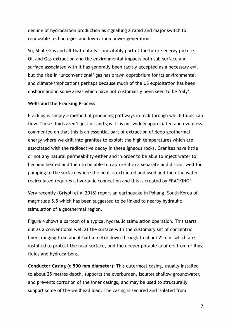
Figure 4 shows a cartoon of a typical hydraulic stimulation operation. This starts

out as a conventional well at the surface with the customary set of concentric

liners ranging from about half a metre down through to about 25 cm, which are

installed to protect the near-surface, and the deeper potable aquifers from drilling

fluids and hydrocarbons.

Conductor Casing (c 500 mm diameter): This outermost casing, usually installed

to about 25 metres depth, supports the overburden, isolates shallow groundwater,

and prevents corrosion of the inner casings, and may be used to structurally

support some of the wellhead load. The casing is secured and isolated from

7

surrounding unconsolidated deposits by a cement caisson, which extends to ground

surface.

Figure 4 The Casing structure and the geometry of a hydraulic stimulation

(fracking) process. Note that this is NOT to scale and that fracking

typically occurs at c 3 km (10,000 feet) (Sundry sources) as shown by

the multiple Empire State Buildings shown on the left.

Surface Casing c 350 mm diameter: After the conductor casing has been drilled

and cemented, the surface casing is installed to an appropriate depth below the

deepest potable aquifer to protect groundwater. Pressure integrity tests are

conducted at this stage:

• Casing pressure test: to test whether the casing integrity is adequate

• Formation pressure integrity test (FIT): is performed to ensure the

cement job has provided a complete seal and provide an assessment

of the strength of the rock formation in that zone.

8

• A cement bond log (CBL) is also conducted using a sonic tool to

confirm the presence and the quality of the cement bond between

the casing and the formation along the entire cemented section of

the well bore.

N.B. CBLs can also be undertaken during the life of the well to confirm

integrity.

Intermediate Casing – c 250 mm diameter: The purpose of the

intermediate casing is "to isolate subsurface formations that may cause

borehole instability and to provide protection from abnormally pressured

subsurface formations" (API, 2009). It is cemented either to the ground

surface or to above any drinking water aquifer or hydrocarbon bearing zone.

Casing pressure and formation pressure integrity tests ensure the casing and

seal integrity.

Production Casing – c 180 mm diameter: The production casing extends

from the surface all the way into the natural gas producing zone isolating it

from all other subsurface formations and allows pumping the HF fluids into

the target zone without affecting other hydrogeological units and then

provides the conduit for natural gas and flowback fluid recovery once

fracturing is completed. The production casing is pressure tested to ensure

well integrity prior to perforating the casing within the hydrocarbon bearing

zone and performing the HF stage.

Petroleum wells therefore consist of a series of concentric steel casings and

cement layers. This practice ensures that robust cement integrity exists

across casing shoes providing complete zonal isolation in the wellbore.

Casings are similarly tested and can also be repaired during the life of

the well and a minor defect, which may be a reportable incident and

9

then appear in statistical estimates as ‘well failure’ should not be seen as

a catastrophic or irrecoverable failure.

Many issues associated with shale gas have been postulated and are shown in

Figure 5

Does the fracking process:

1. Cause contamination of hydrogeological sources, i.e. aquifers, with

fracking fluid from deep hydraulic fractures

2. Cause contamination of surface potable water with fracking fluid and

especially methane from poorly constructed wells and surface spills

3. Cause overwhelming visual and infrastructural impacts

4. Pose a serious risk of damaging seismicity

5. Pose health threats either short-term or long-term

6. Pose a threat to water resources in term of usage

7. Threaten our ability to manage carbon budgets in order to stabilise

climate change

The answers to these questions are often: ‘it rather depends on what you

mean………’ and research suggest that answers to many of these questions are likely

to be NO if the process is done right, in the right geological conditions but this is

not the main substance of this report

prior to Hydrofracturing, the well is plugged using standard cement plugs to isolate the

wellbore below the target zone. Production zones are accessed by perforating the

production casing and surrounding cement of the well with small holes c 3 mm in

diameter, typically along four sides facing the target formation using a perforating gun

designed to make tiny holes through the casing, cementing, and any other barrier between

the formation and the well. Within each zone there are up to 6-7 clusters of small holes

with 6-7 perforations in each cluster. The perforations allow injection of the HF treatment

10

into the rock reservoir and the subsequent flow back of spent HF fluid, produced water

from the formation and hydrocarbons into the well and up to surface.

and the arguments will be confined to addressing Item 4 concerning seismicity.

Figure 5. Postulated Routes to Environmental impact from the Shale Gas

Hydraulic Fracturing operations. (UK Environment Agency)

N.B. Just because a route is illustrated here does NOT necessarily

mean that it IS an environmental threat.

In some cases, a "mini-frac" treatment, a Dynamic Fracture Impedance Test or

DFIT, utilizing a small volume of HF fluid, is initially conducted to collect

diagnostic data about rock strength. stress magnitudes and orientations, which are

then used to refine the computer modelling results and to optimise the HF

execution plan.

The HF process is designed and conducted in a series of sequenced pumping

stages, at pressures of up to c 10000psi (c 700 bars) typically over a period of 2-5

hours in order to produce a series of usually vertical fractures which enhance the

11

permeability and achieve stimulation of the formation to form conduits which can

release and permit the transport of gas and other hydrocarbons into the well.

Volumes are typically of the order of 500,000 US Gallons of fracking fluid which

consists principally of water and sand but with minor amounts of other chemicals.

If the pressure is released the fractures will close and so either silica sand or

proprietary ceramic equivalents are emplaced into the fractures to prop them

open and ensure a permeable transport path.

The fracking will usually begin at the furthest distance from the well and will

progressively move closer in a sequence of stages to produce a wide zone of

stimulated rock. It may seem as if this is a process, which is carried out at such a

distance below ground that it will be difficult, if not impossible, to know where,

and how big the fractured zone is but in fact this isn’t the case. Each tiny fracture

which propagates and eventually coalesces to give the stimulated network emits a

burst of seismic energy, a microseismic event, which carries with it knowledge of

where the fracture is, what its orientation is and how large a fracture has

developed.

Figure 6 Microseismic clouds for a sequence of stimulations, which start at the

furthest extent of the casing (left) and progressively work inwards.

12

The horizontal and vertical extents of the fractures are clearly

delineated by this micro seismicity. (Schlumberger 2007)

Figure 6, shows the microseismic event clouds from a series of seven hydraulic

fracturing stages showing how they extend away from the well laterally and both

upwards and downwards to varying distances which we will see are determined by

local stresses and rock strengths. When fracking is complete it is then possible to

flowback the injected fluid which must be either (and preferably) treated and re-

used or disposed of in a controlled and regulated manner (of which more later) and

the operator can start to extract gas and /or other shale generated hydrocarbons.

There are essentially two families of fracking, ‘slickwater fracking’ which as the

name implies uses relatively low viscosity slippery fluids which can penetrate

easily into rock for significant distances and ‘gel fracking’ which uses more viscous

gels which are often formed with other liquids such as propane or as gas foams

with Carbon Dioxide and Nitrogen. It may sound environmentally foolish to use a

hydrocarbon to frack but as we are trying to recover hydrocarbons it is just part of

the product and can be recovered. These gases including Carbon Dioxide of which

we have too much dispersed in the atmosphere are actually expensive to obtain in

pure form for these purposes and the jury is still out as whether these are more

efficient/economic/environmentally preferable. These are shown in Figure 7:

Figure 7 Gel and slickwater fracking

13

So, we have injected water at sufficiently high pressure to overcome the weight of

the rock above which is typically equivalent to about 10,000 psi. A network of

anatomising fractures has been produced extending away from the wellbore.

If we now reduce the pressure in a process called flowback and do nothing else,

these fractures will immediately close under the huge lithostatic (rock weight)

pressure! Therefore, something must be done to keep these fractures open while

still permitting gas to flow through them and this where proppant comes in. This is

often just well-rounded particles of silica sand which pack and still leave pathways

for gas flow but can also be specially created coated ceramic spheres which are

more expensive but are more resistant to crushing by the high pressure in the

fracture. 99.5% fracking fluid is composed of water and proppant; It is important

to appreciate that the presence of faults or fractures does not necessarily imply

that they are conduits for transport of water/gas/oil or dissolved materials. In

most case these fractures are of low hydraulic conductivity due to their irregular

surfaces, their significant normal confining stresses and the presence of clay

minerals created doing the faulting process (gouge) or precipitation of minerals of

various kinds including calcite and quartz which seal the fault. If it were not so the

hydrocarbons which we would like to access would long ago have escaped to the

surface and disappeared and in fact this is may be true of a fair proportion of the

resource which was once there as we see seeps of hydrocarbons at the surface in

many part of the world.

In fact, we have a pretty good handle on the height to which fractures can go from

the microseismic monitoring which we discussed previously and Figure 8 show this

in two ways. The main figure shows the depth of aquifers in the Barnett are of

Texas which are extensive and extend to more than 1000 feet (300+ metres) but

also the extent of the fractures both above and below the well. The inset shows

that rarely rise more than 300 metres and rarely extend below 200 metres from

the well and Davies et al (2012) have shown that there is a negligible chance of a

hydraulic fracture extending more than 600 metres and in the UK, this has become

the de-factor standard for the respect distance between fracking and overlying

aquifers, i.e. c 2000 feet). This is discussed in some detail later.

14

Figure 8. Vertical extent of hydraulically stimulated fractures with respect to

aquifers and to the casing position (inset). After Warpinski et al (2012) and Maxwell

(pers. comm).

15

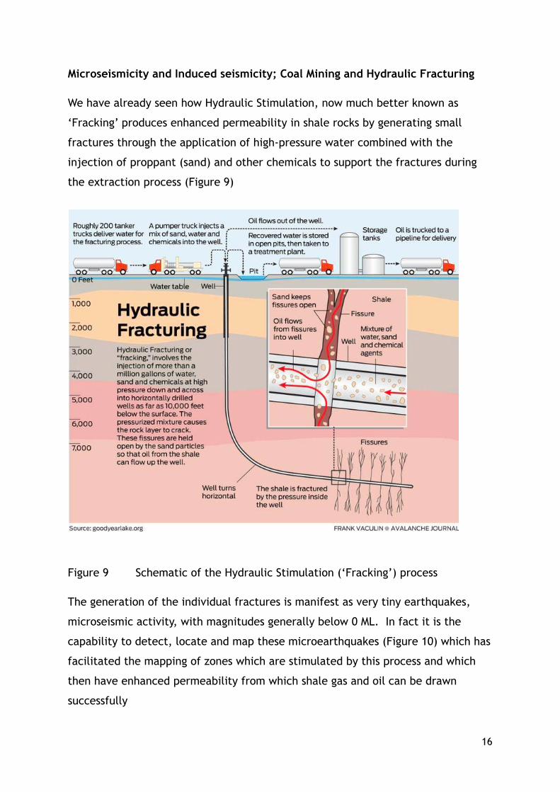
Microseismicity and Induced seismicity; Coal Mining and Hydraulic Fracturing

We have already seen how Hydraulic Stimulation, now much better known as

‘Fracking’ produces enhanced permeability in shale rocks by generating small

fractures through the application of high-pressure water combined with the

injection of proppant (sand) and other chemicals to support the fractures during

the extraction process (Figure 9)

Figure 9 Schematic of the Hydraulic Stimulation (‘Fracking’) process

The generation of the individual fractures is manifest as very tiny earthquakes,

microseismic activity, with magnitudes generally below 0 ML. In fact it is the

capability to detect, locate and map these microearthquakes (Figure 10) which has

facilitated the mapping of zones which are stimulated by this process and which

then have enhanced permeability from which shale gas and oil can be drawn

successfully

16

Figure 10 Microseismicity associated with the fracture process from two

adjacent horizontal wells (from Warpinski 2012)

17

These microearthquakes are usually much too small (less than magnitude zero

often) to be perceived by the population even very close to the activity. However,

sometimes, the stress changes and /or the changes in groundwater pressure and

circulation can facilitate movements on pre-existing, often very old, faults with

the generation of larger seismic events, which may be experienced by the

population over much wider geographic areas and this is known as ‘INDUCED

SEISMICITY” which is not in itself unknown from a variety of causes, most notably

in the UK associated with either current or historic coal mining. Shale-gas related

seismicity came to prominence in the UK in 2011 when on April 1st, 2011 a number

of felt seismic events occurred during the very first fracking test at Preesall,

Lancashire (Known now as the Blackpool earthquakes for various reason) by

Cuadrilla Resources with the largest event at 2.3 ML but other subsequent events

of 1.5 ML and lower. Keele University Applied and Environmental Geophysics

Group, together with BGS installed seismometers and monitored the activity over

the relatively short period of operation and showed the relationship between frack

stages and seismic activity and a report was written advising HMG together with a

number of subsequent papers (Green, Styles, Baptie 2012). Shale gas activities

were severely curtailed following this and there has been considerable opposition

from environmental organisations and local public groups about the concept and

its implementation. Rather surprisingly reports from the USA of shale gas induced

events were initially rather limited and despite induced seismicity, purportedly

related to fracking happening in the Horn River Basin in British Columbia in 2009

this was not reported until 2012 after the Blackpool sequence happened (British

Columbia Oil and Gas Commission (2012)). This was reported generally by Styles

and Baptie (2012), in detail by Clarke et al (2014), Styles (2014) and reviewed by a

Royal Society Committee (2012).

Issues associated with the reactivation of faults are very relevant to the

Environment Agency who state:

“Reactivation of faults during hydraulic fracturing could cause loss of fluids

outside of the permitted zone or formation. As well as being contrary to the

permit conditions this could lead to fluid migration to formations that contain

groundwater that requires protection. In some cases, there could be damage to

18

the borehole structure that in some circumstances could conceivably allow loss of

fluids that could impact on groundwater and, in the case of gases, could impact

on air quality”

Mining Induced Seismicity

Because of the very limited amount of monitored fracking which has taken place to

date in the UK, we must look elsewhere for information about how the rocks of

Britain behave when subject to applied stresses. We are fortunate (or unfortunate

depending on perspective) to have been able to detect, monitor and analyze many

thousands of tiny, small and medium earthquakes and microseismicity from Coal

Mining and I have been carrying out work in this area for some 40 years now. A

review of Anthropogenic Seismicity in the UK can be found in Wilson et al (2017).

Mining Induced Seismicity, i.e. small (usually) earthquakes generated by the

extraction of coal have been reported globally and of more relevance in the UK

since the 1900s soon after long-wall coal mining replaced pillar and stall mining as

the preferred mode of extraction.

I have written extensively about this in many publications (e.g. Styles et al 1997)

and the microseismicity patterns are not very different (although occurring at

much shallower depths) from those associated with fracking, with a relatively

narrow zone of deformation some few hundred metres wide, concentrated around

a coal-face (fracking location) . While mining induced earthquakes have raised

publication apprehension as they can reach magnitude of c 3ML they have

generally been accepted, together with subsidence, as a part of the price of

obtaining one of the main UK energy resources over previous centuries and if

damage was done then compensation was available (NCB and then Coal Authority)

to mitigate the loss. Similar subsidence, if not seismicity is associated with brine

extraction especially in Cheshire and North Yorkshire and was also compensated by

the Brine Compensation Board

While at Swansea, Liverpool and latterly at Keele University I, with my research

groups and graduate students, have had the opportunity through many research

grants both from the UK and Europe (ECSC) to monitor several coal fields in

considerable detail and to be able to generate images of the microseismicity from

19

Thoresby, Edwinstowe, Coventry and most recently, albeit some ten years ago of

Asfordby Colliery and of course around Keele University in the Potteries.

Some images from that monitoring are shown in Figures 11 a, b, c, d .

In the Potteries areas of Stoke, Newcastle-under-Lyme and surrounding areas of

North Staffordshire, coal has been worked extensively from a number of seams to

some considerable depths (c 1100m) and one of the consequences together with

considerable surface subsidence and the reactivation 0f faults (more on this later)

has been very extensive felt seismicity which is shown in Figure 11a with an event

of 2.4 ML , larger than the Blackpool seismic events but which did not generate a

great deal of local concern!! (The good citizens of Stoke are more Stoical than

Blackpool!?)

However, in a ‘well-behaved’ coal mine the microseismic activity remains

relatively closely defined and can be shown to be much as predicted by numerical

models of the stress changes around the excavated zone and extending into the

roof and also the floor of the mine. The event size is again very, very tiny usually

with magnitudes below zero and in some case down to -3 and -4 ML. This is show in

20

Figure 11b from in-seam monitoring of Coventry Colliery. The similarity between

this and the patterns of ‘well-behaved fracking as shown in Figure 10 are clear.

However, it is not always possible to obtain what is known as ‘roof control’ and this

appears to be often related to the presence of pre-existing geological

discontinuities, most notably faults, when stress changes precipitate movement

some considerable distance away from where it might be expected and often with

seismic events which are much larger and sometime felt by populations.

In the early 1990s significant felt seismicity was reported from the Thoresby region

of the North Nottinghamshire coalfield and we monitored this with a large network

of surface seismometers and published a paper on it (Bishop and Styles, 1993) and

this will be discussed at some length later but the distribution of the seismicity is

shown in Figure 11c

Asfordby Colliery (Figure 11d) is one of those locations where mining was

associated with seismicity which occurred on faulting high above the zone of

mining and eventually led to the premature closure of what was a very expensive

mine to open and which had been expected to be a major contributor to UK coal

extraction. Monitoring at that time while technically of a high order and with very

refined detection capabilities was generally done in retrospect with later analysis

of the data and its interpretation in terms of mining operations’.

Figure 11a Seismicity recorded in the Potteries associated with Coal Mining

including a magnitude 2.4 ML event (larger than the largest Blackpool Earthquake!)

21

Figure 11b Microseismicity recorded using in-seam techniques from

Coventry Colliery (Styles et al 1997)

22

-500 -400 -300 -200 -100-150

-100

-50

0

50

100

150

200

y (m)

Heig

ht re

lativ

e to

sea

m (m

)

Sectional view, face advance to right

-100 0 100 200 300-500

-400

-300

-200

-100

x (m)

y (m

)

Plan

-100 0 100 200 300-150

-100

-50

0

50

100

150

200

x (m)

Heig

ht re

lativ

e to

sea

m (m

)

Sectional view, face advance into page

-100 0 100 200 300-400

-200

-100

0

100

200

x (m)

3D view

y (m)

Heig

ht re

lativ

e to

sea

m (m

)

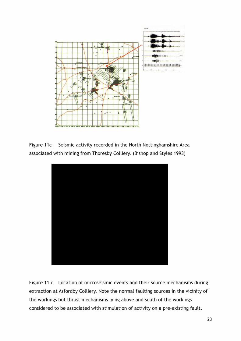
Figure 11c Seismic activity recorded in the North Nottinghamshire Area

associated with mining from Thoresby Colliery. (Bishop and Styles 1993)

Figure 11 d Location of microseismic events and their source mechanisms during

extraction at Asfordby Colliery, Note the normal faulting sources in the vicinity of

the workings but thrust mechanisms lying above and south of the workings

considered to be associated with stimulation of activity on a pre-existing fault.

23

We can see that the onset of stimulation of activity on pre-existing faults, as

opposed to new fractures is generally associated with an increase in magnitude

often of several orders and this has been noted for fracking operations in the USA

(Figure 12) albeit still at extremely low magnitudes of less than 0.5ML.

Figure 12 Microseismicity and its increase in magnitude as pre-existing faults

are stimulated. Examples from the Barnett Shale.

24

Shale Gas, Fracking and Seismicity in the United Kingdom

Figure 13 shows the relationship between the Bowland Shale and the

Coal Measures. It lies beneath the Westphalian coals and shales of the

Coal Measures in the rocks of Namurian (Millstone Grit) and Dinantian

ages both of which overly the Carboniferous Limestone (Frazer and

Gawthorpe 1990). In many areas, the Bowland Shale is found within a

few hundred metres of worked coal seams.

Figure 13 Stratigraphical position of the Bowland Shale with respect to

the Coal Measures (BGS)

25

Figure 14 show the first fracked well for shale gas in the United Kingdom which

commenced in March 2011 and Table 1 shows the fracking stages which took place.

Figure 14. Cuadrilla Preese Hall 1 Borehole and its location in the Bowland Basin

which clearly also extends offshore into the Irish Sea.

Table 1 Fracking Stages carried out in Preese Hall 1

26

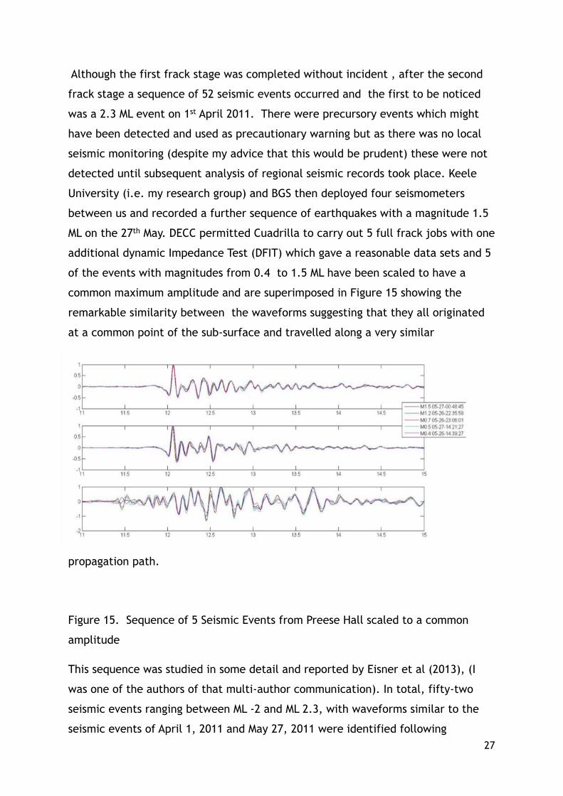
Although the first frack stage was completed without incident , after the second

frack stage a sequence of 52 seismic events occurred and the first to be noticed

was a 2.3 ML event on 1st April 2011. There were precursory events which might

have been detected and used as precautionary warning but as there was no local

seismic monitoring (despite my advice that this would be prudent) these were not

detected until subsequent analysis of regional seismic records took place. Keele

University (i.e. my research group) and BGS then deployed four seismometers

between us and recorded a further sequence of earthquakes with a magnitude 1.5

ML on the 27th May. DECC permitted Cuadrilla to carry out 5 full frack jobs with one

additional dynamic Impedance Test (DFIT) which gave a reasonable data sets and 5

of the events with magnitudes from 0.4 to 1.5 ML have been scaled to have a

common maximum amplitude and are superimposed in Figure 15 showing the

remarkable similarity between the waveforms suggesting that they all originated

at a common point of the sub-surface and travelled along a very similar

propagation path.

Figure 15. Sequence of 5 Seismic Events from Preese Hall scaled to a common

amplitude

This sequence was studied in some detail and reported by Eisner et al (2013), (I

was one of the authors of that multi-author communication). In total, fifty-two

seismic events ranging between ML -2 and ML 2.3, with waveforms similar to the

seismic events of April 1, 2011 and May 27, 2011 were identified following 27

injections on 31st of March and the 26th and 27th of May with remarkably low

seismic activity in the period between and after injections. Only two weak events

(M -1.2 and -0.2) were found after May 27, 2011 until 2 August 2011 when another

event of magnitude less than 0.0 ML occurred, indicating a rapid decline in

seismicity after the end of the injections, another indication of causality. Similarly,

only three weak events were observed between the two injection periods and no

event was detected during the stimulation of the stage 3. The detection threshold

had been improved by the installation of the local Keele and BGS stations on April

12, 2011 and so it is clear that the catalogue from the regional stations is complete

down to ML 0. The event of August 2nd 2011 was very similar to the May 27th

event(s) indicating that there was still some residual if small readjustment taking

place on the fault and the orientation was determined with reasonable accuracy

despite the small magnitude as strike, dip and rake 40o; 70o; and -150o, , a steeply

dipping fault oriented more or less SW-NE in agreement with the main regional

fault trends as seen in Figure 14. Analysis of data from the regional station KESW

(Keswick) showed that there had been 6 small events of magnitude exceeding 0.2

ML prior to the larger event of 1st April, but during the early part of the hydraulic

fracturing when pressures were above 7000 psi.

When we look at the events of 26th and 27th May 2011 (Table 2) in Time sequence

rather than in Magnitude sequence as in Figure 15 we can see that the first

movement on this fault (with the assumption that all of these lie on the same fault

which is justified by the similarity of the waveforms) we see that the first

indication was an event of magnitude only 0.4ML, followed by a larger event of 1.2

ML some 8 hours later and then in reasonably close succession events of 0.7 and

1.5ML just before and after midnight on the 26/27 May 2011. A final event of

magnitude 0.5 occurred later in the afternoon of 27th May

28

Table 2. Five large events of 26th and 27th May 2011 arranged in order of

temporal occurrence

Day Month Year Min Sec Magnitude

26 5 2011 14 39 0.4

26 5 2011 22 35 1.2

26 5 2011 23 6 0.7

27 5 2011 0 48 1.5

27 5 2011 14 21 0.5

29

The implications are that a small event of magnitude 0.4 (with a downwards first

P-Wave motion on the vertical component shown in the lower plot) was the initial

indication that this fault was being stimulated and then the subsequent larger

events, indicating that a longer length of the fault was being stimulated, have an

upwards first P-wave motion.

Subsequent seismic reflection surveying (they were also advised by me to do this

prior to fracking as well!) showed that it was likely that the fracking stimulated a

fault, a few hundred metres ahead of the frack point (Figure 16).

Figure 16. 3-D Seismic reflection data showing the relationship between the

wellbore and the fault which was presumed to be the location of the induced

seismicity. (Cuadrilla)

I was asked to be part of a team examining the events and reporting to DECC

(Green, Styles, Baptie 2012) and in this lengthy report we proposed the following:

We recommend a detailed analysis of potential seismic

hazards prior to spudding the well. This should include:

o Appropriate baseline seismic monitoring to establish background

seismicity in the area of interest.

o Characterisation of any possible active faults in the region using

all available geological and geophysical data

o Application of suitable ground motion prediction models to assess

the potential impact of any induced earthquakes

We will return to this recommendation later but note that the Canadian

Regulations also recommend

• Assess faults, lineations, background seismicity and other possible

cases of induced seismicity in the area

Based on the work of Warpinski et al (2011) in the USA we noted that there seemed

to be a distinct change in seismic character at about 0.5 ML as shown in the

30

following two figures 17 and 18 and suggested that this point should be the level at

which caution should be applied to the fracking operations.

The UK Government (DECC now BEIS) decided that the 0.5 ML limit (Figure 19)

should be THE stopping point at which fracking activities should be suspended

against our advice that 1.5 ML would be a more appropriate threshold. This seems

at first glance to be a prudent decision in order to give maximum protection

against significant population disturbing seismicity but as I will explain this has

significant implications concerning the size of faults which are therefore defined

31

to be of significance and the ability of current seismic reflection techniques to

detect faults of those dimensions.

There has been a large body of work done on the relationship between Earthquake

Magnitude and the length of the fault slip which has caused that event (Zoback

2012) and as Figure 20 shows for a 0.5 ML event that length is only just in excess of

25 metres perhaps as large as 40 metres depending on the amount of actual slip

which took place.

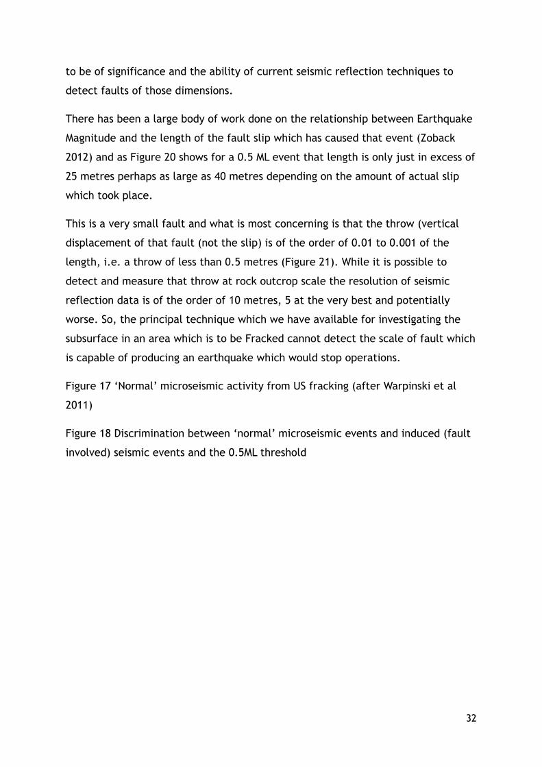
This is a very small fault and what is most concerning is that the throw (vertical

displacement of that fault (not the slip) is of the order of 0.01 to 0.001 of the

length, i.e. a throw of less than 0.5 metres (Figure 21). While it is possible to

detect and measure that throw at rock outcrop scale the resolution of seismic

reflection data is of the order of 10 metres, 5 at the very best and potentially

worse. So, the principal technique which we have available for investigating the

subsurface in an area which is to be Fracked cannot detect the scale of fault which

is capable of producing an earthquake which would stop operations.

Figure 17 ‘Normal’ microseismic activity from US fracking (after Warpinski et al

2011)

Figure 18 Discrimination between ‘normal’ microseismic events and induced (fault

involved) seismic events and the 0.5ML threshold

32

Figure 19. DECC Traffic Light Threshold Regulation.

Figure 20 Fault dimensions for a variety of Earthquake magnitudes (after

Zoback and Gorelick 2010)

33

Figure 21. Relationship between Fault Length and Fault throw for faults

measured underground in the East Pennine Coalfield (Bailey et al.

2002)

Respect Distances

Subsequent to this work, Professor Richard Davies (Durham) and myself, Professor

Peter Styles (Keele) were asked by the Prime Minister’s Office (David Cameron as

was) to make recommendations as to the vertical (from aquifers) and horizontal

(from faults) distances, which we considered, should be observed for incident free

fracking. Those recommended respect distances are shown in Figure 22 and are

600 metres vertically beneath an aquifer and 850 metres horizontally from a fault.

Note that implementation of this requires the detection and mapping of the

appropriate faults which on the basis of the previous discussion should include

those which might give rise to a 0.5 ML earthquake i.e. 40 metres long and with

a 0.5 to 1 metre throw!!!.

34

Figure 22 Respect Distances as advised to no. 10 Downing Street in February 2015.

(Davies and Styles 2015 pers. comm.)

A subsequent paper by Wilson et al (2018) has confirmed this as an appropriate set

of respect distances.

Figure 23. BGS Estimates of the principal resource areas for shale gas in the

North of England. (BGS and Smith, Turner and Williams 2011)

35

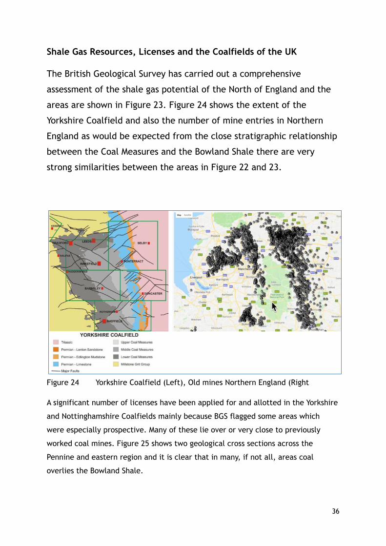
Shale Gas Resources, Licenses and the Coalfields of the UK

The British Geological Survey has carried out a comprehensive

assessment of the shale gas potential of the North of England and the

areas are shown in Figure 23. Figure 24 shows the extent of the

Yorkshire Coalfield and also the number of mine entries in Northern

England as would be expected from the close stratigraphic relationship

between the Coal Measures and the Bowland Shale there are very

strong similarities between the areas in Figure 22 and 23.

Figure 24 Yorkshire Coalfield (Left), Old mines Northern England (Right

A significant number of licenses have been applied for and allotted in the Yorkshire

and Nottinghamshire Coalfields mainly because BGS flagged some areas which

were especially prospective. Many of these lie over or very close to previously

worked coal mines. Figure 25 shows two geological cross sections across the

Pennine and eastern region and it is clear that in many, if not all, areas coal

overlies the Bowland Shale.

36

Figure 25 Geological Cross- Sections across Derbyshire and Yorkshire (BGS)

I have looked at a number of these applications and they, probably as they have

been advised, have used BGS geological maps and existing seismic reflection data

of early vintage (BP acquired mostly) to formulate their planning applications. BGS

surface fault maps are excellent but are limited as to the scale of faulting they

show and as I have previously explained in detail surface seismic reflection

CANNOT resolve the scale of faulting which might give rise to seismic events which

would curtail shale gas operations.

However, it does not seem to have been noted that all coal mined areas in the era

of the National Coal Board (and probably earlier) were mapped in great detail (a

37

few tens of centimetre scale) underground because of mine safety and in order to

track the changes in seam level as faults were crossed and mine fault maps exist in

the archives of the Coal Authority. Before I took the Chair of Geophysics at Keele

University in 2000 from 1988 to 2000 I was Senior Lecturer and then Reader in

Geophysics and led the Applied Geophysics Research Group at Liverpool University.

While there I worked closely with the Fault Analysis Group, led by Professor Juan

Watterson and then by Dr John Walsh (now Professor John Walsh of Dublin

University). Their research was in the statistics of fault distributions which are

fractal in nature.

Figure 26 Spire Slack open-cut coal mine, Central Valley Scotland. Exposed

face at Spire Slack open-cut coal-mine, showing the fracture and

fault networks down to a few cm, which are fractal in nature, with

discontinuities. The exposed face is in the Lower Limestone and is

approximately 50 m high. Some residual coal can be seen in the

foreground

This can clearly be seen in Figure 26, which is of an exposed worked opencast coal

mine face in Scotland which show the intersecting, anastomosing faults over a

wide range of scales present even in a small area. ‘Big Faults have little Faults

upon their backs to bite them and little Faults have lesser Faults and so (almost)

ad infinitum!!’

Bailey et al (2002) of the Fault Analysis Group made a special study of the East

Pennine Coalfield, mapping all faults with throws greater than 1 metre (which

would give an earthquake which would significantly exceed the threshold of

0.5ML!) I have overlain these on the BGS Geological Map (Figure 27) with their BGS

main faults shown in Black and with the underground faults high-lighted in white.

It is clear that there are many, many more faults of significant (seismically) size

than are indicated on even the most detailed BGS maps. Historic and recent

earthquakes are shown as red and white circles from our own studies and those of

the British Geological Survey and it is clear that these fall on or close to these

smaller faults in many cases. While individual faults will vary in definition as they

transfer across different lithologies, i.e. they are much better marked in brittle

38

formations such as Limestones and Sandstones than they are in more ductile

formations such as siltstones and shales, they are clearly important in any

consideration of the structural complexity which is present at any site which is

considering shale gas activities in the vicinity of worked coal seams. As an

example, I show three proposed borehole sites from INEOS licence areas and it is

clear that there are faults much closer to some of the proposed borehole locations

than 850 metres.

Figure 27 Geological Map with Faults (black) from BGS and Faults (highlighted

white) from underground mine maps. Historic Induced seismic events

are shown with white and red dots and fall on the small mapped

faults as well as the large ones and sometimes within a few

kilometres of the proposed boreholes.

It is interesting that Baptie et al (2016) in a report to the Scottish Government on:

39

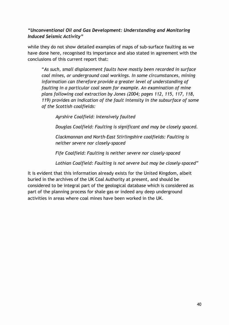
“Unconventional Oil and Gas Development: Understanding and Monitoring Induced Seismic Activity”

while they do not show detailed examples of maps of sub-surface faulting as we have done here, recognised its importance and also stated in agreement with the conclusions of this current report that:

“As such, small displacement faults have mostly been recorded in surface coal mines, or underground coal workings. In some circumstances, mining information can therefore provide a greater level of understanding of faulting in a particular coal seam for example. An examination of mine plans following coal extraction by Jones (2004; pages 112, 115, 117, 118, 119) provides an indication of the fault intensity in the subsurface of some of the Scottish coalfields:

Ayrshire Coalfield: Intensively faulted

Douglas Coalfield: Faulting is significant and may be closely spaced.

Clackmannan and North-East Stirlingshire coalfields: Faulting is neither severe nor closely-spaced

Fife Coalfield: Faulting is neither severe nor closely-spaced

Lothian Coalfield: Faulting is not severe but may be closely-spaced”

It is evident that this information already exists for the United Kingdom, albeit buried in the archives of the UK Coal Authority at present, and should be considered to be integral part of the geological database which is considered as part of the planning process for shale gas or indeed any deep underground activities in areas where coal mines have been worked in the UK.

40

Conclusions

1. Although little seismic data exists from fracking operations in the

UK at present a great deal of coal mining-induced seismicity data

does exist and has a great deal of relevance as it shows that pre-

existing faults can be and have been stimulated by coal mining

and have generated seismic events up to about 3ML.

2. Current UK Seismic Traffic Light Thresholds postulate a cessation

and subsequent modification (or even halting) of fracking

activities if an earthquake of magnitude 0.5 ML occurs. This size

of event corresponds to a movement of only a few millimetres on

a short fault segment of a larger fault or even on an individual

fault of only about 40 metres length and with a throw of less

than a metre which cannot be detected on current seismic

reflection data as part of an exploration programme for Shale

Gas planning and such small faults are not shown on BGS maps.

3. In many areas proposed Shale Gas activities lie beneath historic

coal mine workings which have already experienced subsidence

and sometimes fault rejuvenation. In these mined-out areas

however, we DO have detailed geological information especially

with regard to faulting as this was mapped with high-precision

underground as part of mine safety and for planning.

Indeed: Jones et al (2004) in a comprehensive BGS report on “UK Coal Resource for New Exploitation Technologies Final Report” Sustainable Energy & Geophysical Surveys Programme Commissioned Report CR/04/015N state:

41

Extent of underground workings with 500 m buffer zone. The extent of former underground mine workings was supplied as a digital dataset by the Coal Authority. The data were supplied as comma separated variables representing the workings of one named seam. This was loaded into the ESRI®ArcMapTM (v.8.3) GIS software and a 500 m buffer zone was added to this dataset.

The buffer zone represents a stand-off distance recommended to mitigate against the possible interaction of former mine workings with the other technologies.

4. When this detailed mine mapping data is plotted together with

locations of historic and relatively recent seismic events it is

clear that they lie close to or on these smaller faults in many

instances.

5. These, small but potentially active faults which are capable of

generating seismic events which would exceed the Traffic Light

Thresholds can be seen to occur much closer to proposed

borehole sites than the 850 metres respect distance proposed by

Davies and Styles (2015) to UK Government and Wilson et al

(2018)

6. It is critical that this high resolution, carefully mapped data set

should be included in any planning process for unconventional oil

and gas activities.

42

Professor Emeritus Peter Styles, FGS CGeol., FRAS CSci, FIMMM

2 May 2018

References

Bailey, W. R., Manzocchi, T., Walsh, J. J., Keogh, K., Hodgetts, D., Rippon,

J., Neil. P. A. R, Flint. S., Strand, J. A. (2002). The effect of faults on the 3D

connectivity of reservoir bodies: A case study from the East Pennine

Coalfield, UK. Petroleum Geoscience, 8(3), 263-277.

Baptie B., Segou M., Ellen R. And A. Monaghan. (2016). Unconventional Oil and Gas Development: Understanding and Monitoring Induced Seismic Activity. British Geological Survey Open Report, OR/16/042, 92pp.

Bishop I, Styles P. and Allen M., (1993) Mining-induced seismicity in the

Nottinghamshire Coalfield, Quarterly Journal of Engineering Geology, 26,

253-279.

Clarke, H., L. Eisner, P. Styles, and. P. Turner (2014), Felt seismicity

associated with shale gas hydraulic fracturing: The rst documented example

in Europe, Geophys. Res. Lett., 41, doi:10.1002/2014GL062047

Davies, R., S. Mathias, J. Moss, S. Hustoft, L. Newport. 2012. Hydraulic

fractures: How far can they go? Marine and Petroleum Geology 37(1):1-6.

Davies, R., Foulger, G., Bindley, A. and Styles, P., (2013) Induced seismicity

and hydraulic fracturing for the recovery of hydrocarbons, Mar. Pet. Geol.,

45, 171-185, DOI: 10.1016/j.marpetgeo.2013.03.016

Eisner E., Halló M., Janská E., Opršal I., Matoušek P., Clarke H., Turner P.,

Harper T., Styles P. (2013) , Lessons learned from hydraulic stimulation of

the Bowland Shale, SEG Houston 2013 Annual Meeting, DOI http://

dx.doi.org/10.1190/segam2013-0239.1, Pages 4516-4520.

Ellsworth W.L., 2013. Injection-Induced Earthquakes, Science 341 no. 6142 .

Fraser A. J., and Gawthorpe R. L. (1990), Tectono-stratigraphic development

and hydrocarbon habitat of the Carboniferous in northern England,

Geological Society, London, Special Publications 1990, v. 55, p. 49-86

43

Green, C.A., Styles, P., Baptie, B.J., 2012. Preese Hall Shale Gas

Fracturing: Review and Recommendations for Induced Seismic Mitigation.

Available at: http://www.decc.gov.uk/assets/decc/11/meeting-energy-

demand/oil-gas/5055-preese-hall-shale-gas-fracturing-review-and-

recomm.pdf Accessed 27 October 2012.

Grigoli F., Cesca, S A., Rinaldi A. P., , A. Manconi A, López-Comino J.A.,

ClintonJ. F., Westaway R., Cauzzi C., Dahm T., Wiemer S., (2018)., The

November 2017 Mw 5.5 Pohang earthquake: A possible case of induced

seismicity in South Korea, Science 26 Apr 2018:DOI: 10.1126/

science.aat2010

Jones N. S., Holloway S., Creedy D. P., Garner K., Smith N. J. P., Browne,

M.A.E. & Durucan S. (2004), UK Coal Resource for New Exploitation

Technologies Final Report, Commissioned Report CR/04/015N.

Royal Society and Royal Academy of Engineering. (2012), Shale gas extraction in the UK: a review of hydraulic fracturing. Available at: http://www.royalsociety.org/policy/projects/shale-gas-extraction and raeng.org.uk/shale.

Smith, N, Turner P. and Williams G., (2011), UK data and analysis for shale

gas prospectivity, Geological Society, London, Petroleum Geology

Conference series, 7, 1087-1098, 4 January 2011, https://doi.org/

10.1144/0071087

Styles, P., Flynn Z., and Toon S.M., (1999) Integrated Microseismic

Monitoring and Numerical Modelling for the Determination of Fracture

Architecture Around Longwall Coal Mines for Geomechanical Validation.

ECSC Research Agreement No: 7229-AF/013“Application of Geophysical and

Geodetic Techniques to the Determination of Structure and Monitoring of

the Surface”

Styles., P., (2014) Shale Gas and Hydraulic Fracturing: A Review of the

Environmental, Geological and Climate Risks, Emirates Centre for Strategic

Sustainability Research in “CONVENTIONAL FOSSIL FUELS: The next

hydrocarbon revelation?”, Emirates Centre for Strategic Research, 61pp.

44

Styles P. and Baptie, B., 2012., Induced Seismicity in the UK and its

Relevance to Hydraulic Stimulation for Exploration for Shale Gas., https://

www.gov.uk/government/uploads/system/uploads/attachment_data/file/

48331/5056-background-note-on-induced-seismicity-in-the-uk-an.pdf

Warpinski, N. R., J. Du, and U. Zimmer (2012), Measurements of hydraulic-

fracture-induced seismicity in gas shales, SPE Production and Operations,

27(3), 240-252.

Westwood RF, Toon SM, Styles P, Cassidy NJ. (2017). Horizontal respect

distance for hydraulic fracturing in the vicinity of existing faults in deep

geological reservoirs: A review and modelling study. Geomechanics and

Geophysics for Geo-Energy and Geo-Resources. vol. 3(4), 379-391

Wilson, M. P., Davies, R. J, Foulger G. R., Julian B. R., , Styles P., Gluyas J.

G., Almond S., (2017), Anthropogenic earthquakes in the UK: a national

baseline prior to shale exploitation, Marine and Petroleum Geology,

Published Online August 2015-11-26

Wilson, M. P. and Worrall, F. and Davies, R. J. and Almond, S. (2018)

'Fracking : how far from faults?', Geomechanics and geophysics for geo-

energy and geo-resources. https://doi.org/10.1007/s40948-018-0081-y

Zoback . M. and Gorelick S.M. (2012) Earthquake triggering and large-scale

geologic storage of carbon dioxide, PNAS June 26, 2012. 109 (26)

10164-10168; https://doi.org/10.1073/pnas.1202473109

45