FPGA implementation of PSO algorithm and neural networks

Scholars' Mine Scholars' Mine

Masters Theses Student Theses and Dissertations

Spring 2010

FPGA implementation of PSO algorithm and neural networks FPGA implementation of PSO algorithm and neural networks

Parviz Palangpour

Follow this and additional works at: https://scholarsmine.mst.edu/masters_theses

Part of the Computer Engineering Commons

Department: Department:

Recommended Citation Recommended Citation Palangpour, Parviz, "FPGA implementation of PSO algorithm and neural networks" (2010). Masters Theses. 4759. https://scholarsmine.mst.edu/masters_theses/4759

This thesis is brought to you by Scholars' Mine, a service of the Missouri S&T Library and Learning Resources. This work is protected by U. S. Copyright Law. Unauthorized use including reproduction for redistribution requires the permission of the copyright holder. For more information, please contact [email protected].

https://library.mst.edu/

https://library.mst.edu/

https://scholarsmine.mst.edu/

https://scholarsmine.mst.edu/masters_theses

https://scholarsmine.mst.edu/student-tds

https://scholarsmine.mst.edu/masters_theses?utm_source=scholarsmine.mst.edu%2Fmasters_theses%2F4759&utm_medium=PDF&utm_campaign=PDFCoverPages

http://network.bepress.com/hgg/discipline/258?utm_source=scholarsmine.mst.edu%2Fmasters_theses%2F4759&utm_medium=PDF&utm_campaign=PDFCoverPages

https://scholarsmine.mst.edu/masters_theses/4759?utm_source=scholarsmine.mst.edu%2Fmasters_theses%2F4759&utm_medium=PDF&utm_campaign=PDFCoverPages

mailto:[email protected]

FPGA IMPLEMENTATION OF PSO ALGORITHM AND NEURAL NETWORKS

by

PARVIZ MICHAEL PALANGPOUR

A THESIS

Presented to the Faculty of the Graduate School of the

MISSOURI UNIVERSITY OF SCIENCE AND TECHNOLOGY

In Partial Fulfillment of the Requirements for the Degree

MASTER OF SCIENCE IN COMPUTER ENGINEERING

2010

Approved by

Ganesh Kumar Venayagamoorthy, AdvisorWaleed Al-AssadiMaciej Zawodniok

c� 2010

PARVIZ MICHAEL PALANGPOUR

All Rights Reserved

iii

ABSTRACT

This thesis describes the Field Programmable Gate Array (FPGA) implemen-

tations of two powerful techniques of Computational Intelligence (CI), the Particle

Swarm Optimization algorithm (PSO) and the Neural Network (NN).

Particle Swarm Optimization (PSO) is a popular population-based optimiza-

tion algorithm. While PSO has been shown to perform well in a large variety of

problems, PSO is typically implemented in software. Population-based optimization

algorithms such as PSO are well suited for execution in parallel stages. This allows

PSO to be implemented directly in hardware and achieve much faster execution times

than possible in software. In this thesis, a pipelined architecture for hardware PSO

implementation is presented. Benchmark functions solved by software and FPGA

hardware PSO implementations are compared.

NNs are inherently parallel, with each layer of neurons processing incoming

data independently of each other. While general purpose processors have reached

impressive processing speeds, they still cannot fully exploit this inherent parallelism

due to their sequential architecture. In order to achieve the high neural network

throughput needed for real-time applications, a custom hardware design is needed. In

this thesis, a digital implementation of an NN is developed for FPGA implementation.

The hardware PSO implementation is designed using only VHDL, while the NN

hardware implementation is designed using Xilinx System Generator. Both designs

are synthesized using Xilinx ISE and implemented on the Xilinx Virtex-II Pro FPGA

Development Kit.

iv

ACKNOWLEDGMENT

I am deeply grateful to my advisor Dr. Ganesh Kumar Venayagamoorthy, who

has provided me with guidance, knowledge and financial support throughout the

research and preparation of this thesis.

I would also like to thank Dr. Waleed Al-Assadi and Dr. Maciej Zawodniok for

their assistance and serving on my committee. I would also like to thank Dr. Scott

C. Smith for his advice and comments towards my work.

I would like acknowledge funding from the following grants:

1. GAANN: Advanced Computational Techniques and Real-Time Simulation Stud-

ies for the Next Generation Energy Systems

2. NSF CAREER: Scalable Learning and Adaption with Intelligent Techniques

and Neural Networks for Reconfiguration and Survivability of Complex Systems

(ECCS # 0348221)

3. EFRI-COPN: Neuroscience and Neural Networks for Engineering the Future

Intelligent Electric Power Grid (EFRI #0836017)

Most importantly, I would like to thank my parents for their unconditional

support and encouragement towards reaching my goals.

v

TABLE OF CONTENTS

Page

ABSTRACT . . . . . . . . . . . . . . . . . . . . . . . . . . . . . . . . . . . . iii

ACKNOWLEDGMENT . . . . . . . . . . . . . . . . . . . . . . . . . . . . . . iv

LIST OF ILLUSTRATIONS . . . . . . . . . . . . . . . . . . . . . . . . . . . . vii

LIST OF TABLES . . . . . . . . . . . . . . . . . . . . . . . . . . . . . . . . . ix

SECTION

1 INTRODUCTION . . . . . . . . . . . . . . . . . . . . . . . . . . . . . 1

1.1 BACKGROUND . . . . . . . . . . . . . . . . . . . . . . . . . . . . 1

1.2 THESIS OBJECTIVE . . . . . . . . . . . . . . . . . . . . . . . . . 4

1.3 THESIS OVERVIEW . . . . . . . . . . . . . . . . . . . . . . . . . 4

1.4 CONTRIBUTIONS OF THIS THESIS . . . . . . . . . . . . . . . 5

1.5 RESEARCH PUBLICATIONS . . . . . . . . . . . . . . . . . . . . 5

1.6 SUMMARY . . . . . . . . . . . . . . . . . . . . . . . . . . . . . . 5

2 IMPLEMENTATIONS OF PSO ALGORITHM . . . . . . . . . . . . . 6

2.1 INTRODUCTION . . . . . . . . . . . . . . . . . . . . . . . . . . . 6

2.2 PARTICLE SWARM OPTIMIZATION . . . . . . . . . . . . . . . 7

2.3 PSO HARDWARE IMPLEMENTATION . . . . . . . . . . . . . . 9

2.3.1 The Hardware Velocity Update. . . . . . . . . . . . . . . . . . . 10

2.3.2 Random Number Generation. . . . . . . . . . . . . . . . . . . . 11

2.3.3 Control Module. . . . . . . . . . . . . . . . . . . . . . . . . . . 12

2.4 RESULTS . . . . . . . . . . . . . . . . . . . . . . . . . . . . . . . 13

3 IMPLEMENTATION OF NEURAL NETWORK . . . . . . . . . . . . 19

3.1 INTRODUCTION . . . . . . . . . . . . . . . . . . . . . . . . . . . 19

3.2 DESIGN APPROACH . . . . . . . . . . . . . . . . . . . . . . . . 20

3.3 NN HARDWARE IMPLEMENTATION . . . . . . . . . . . . . . . 21

vi

3.3.1 Implementing the Neuron MAC. . . . . . . . . . . . . . . . . . 21

3.3.2 Implementing the Activation Function LUT. . . . . . . . . . . . 23

3.3.3 Implementing the Complete Hardware Neuron. . . . . . . . . . 24

3.3.4 Implementing the NN Layer Control Block. . . . . . . . . . . . 26

3.3.5 Implementing a Three-Layer NN. . . . . . . . . . . . . . . . . . 27

3.4 RESULTS . . . . . . . . . . . . . . . . . . . . . . . . . . . . . . . 30

4 CONCLUSIONS AND FUTURE WORK . . . . . . . . . . . . . . . . . 35

APPENDICES

A HARDWARE PSO SOURCE CODE. . . . . . . . . . . . . . . . . . . . 36

B HARDWARE NN SOURCE CODE. . . . . . . . . . . . . . . . . . . . 67

BIBLIOGRAPHY . . . . . . . . . . . . . . . . . . . . . . . . . . . . . . . . . 76

VITA . . . . . . . . . . . . . . . . . . . . . . . . . . . . . . . . . . . . . . . . 79

vii

LIST OF ILLUSTRATIONS

Figure Page

2.1 PSO hardware implementation with 6-stage pipeline. . . . . . . . . . . . 10

2.2 An example of a linear-feedback shift register. . . . . . . . . . . . . . . 11

2.3 The structure of the neighborhood-of-four PRNG. . . . . . . . . . . . . 12

2.4 The hardware PSO execution flowchart. . . . . . . . . . . . . . . . . . . 14

2.5 A two-dimensional view of the sphere benchmark problem fitness surface. 15

2.6 A two-dimensional view of the Rosenbrock benchmark problem fitnesssurface. . . . . . . . . . . . . . . . . . . . . . . . . . . . . . . . . . . . . 16

2.7 The hardware PSO compared with a software PSO for the sphere functionof 10 dimensions. . . . . . . . . . . . . . . . . . . . . . . . . . . . . . . 17

2.8 The hardware PSO compared with a software PSO for the Rosenbrockfunction of 10 dimensions. . . . . . . . . . . . . . . . . . . . . . . . . . 18

3.1 An NN with an input, hidden and output layer. . . . . . . . . . . . . . 19

3.2 A diagram of the neuron model. . . . . . . . . . . . . . . . . . . . . . . 22

3.3 MAC hardware subsystem. . . . . . . . . . . . . . . . . . . . . . . . . . 22

3.4 LUTAF approximation. . . . . . . . . . . . . . . . . . . . . . . . . . . . 25

3.5 LUTAF approximation subsystem. . . . . . . . . . . . . . . . . . . . . . 25

3.6 The complete hardware neuron. . . . . . . . . . . . . . . . . . . . . . . 26

3.7 The LCB finite state machine (2× 3 Layer). . . . . . . . . . . . . . . . 27

3.8 A LCB controlling three hardware neurons (2× 3 Layer). . . . . . . . . 28

3.9 A hardware neuron being controlled by a LCB. . . . . . . . . . . . . . . 29

3.10 A FPGA-based NN (of size 1× 3× 1). . . . . . . . . . . . . . . . . . . 29

3.11 The trained NN for approximating a sin function. . . . . . . . . . . . . 30

3.12 The output of the Simulink simulation of the FPGA-based NN. . . . . . 32

3.13 Comparing the output of hidden neurons of the FPGA-based NN andMatlab-based NN. . . . . . . . . . . . . . . . . . . . . . . . . . . . . . . 33

3.14 Comparing the output of the FPGA-based NN and Matlab-based NN. . 34

viii

3.15 The hardware resources used for the 1×10×1 NN on the Xilinx Virtex-IIPro FPGA. . . . . . . . . . . . . . . . . . . . . . . . . . . . . . . . . . . 34

ix

LIST OF TABLES

Table Page

2.1 The values for the LUT in each PRNG cell. . . . . . . . . . . . . . . . . 13

2.2 Achieved fitness after 1000 iterations for benchmark problems. . . . . . 17

2.3 Execution time for software and hardware PSO implementations. . . . . 17

2.4 Hardware PSO logic requirements for the benchmark problems. . . . . . 18

3.1 The values for the hyperbolic tangent activation Function LUT wherex ∈ [L, U ]. . . . . . . . . . . . . . . . . . . . . . . . . . . . . . . . . . . 24

1 INTRODUCTION

1.1 BACKGROUND

Computational Intelligence (CI) is a sub-branch of artificial intelligence. CI

is the study of adaptive mechanisms to enable or facilitate intelligent behavior in

complex and changing environments [1]. Many of the CI paradigms have mechanisms

that exhibit the ability to adapt to new situations, to generalize, abstract, discover and

associate. The main CI paradigms are artificial Neural Networks (NNs), evolutionary

computing, Swarm Intelligence (SI) and fuzzy systems. Each of these paradigms

has origins in some biological system. For instance, NNs are models of biological

neural systems while SI models the social behavior of organisms that live in swarms

or colonies.

The most common way to implement CI techniques is to write software that

can be executed on a standard digital processor. One reason why this approach is the

most common is because of the ease of development as developers can take advantage

of the enormous number of existing software libraries. By building applications on

top of existing software libraries and operating systems, the developer can implement

the application without having to be concerned with the operation of the underlying

digital hardware. Furthermore, there are a large number of software programming

languages available, C, C++, Java, etc; for each of these languages exists multi-

ple mature tools exist that make implementing, simulating and optimizing software

applications much easier.

There are also a variety of digital processors that can be used to execute CI

software, microcontrollers, digital signal processors (DSPs) and general purpose mi-

croprocessors. Microcontrollers offer the least amount of processing power but are

available at very low prices and consume very little power. DSPs are designed specif-

ically for digital signal processing applications while general purpose microprocessors

offer the highest performance and flexibility. When software is compiled for execu-

tion on a specific processor, the compiler essentially converts the software into series

of small instructions. These instructions are then executed in a sequential nature

on the processor. However, only the simplest of processors execute instructions in a

2

strictly sequential manner, more advanced processors utilize different techniques to

achieve instruction-level parallelism that allow the execution of multiple instructions

simultaneously.

While the trend in high-performance microprocessor and DSP design is to incor-

porate techniques to achieve instruction-level parallelism, the processor and software

compiler are left to interpret and exploit any such opportunities for parallelism. As

processors are designed for general purpose computing, they cannot be designed to

take advantage of the underlying parallelism in each application. Instead of executing

the software on a processor, a custom digital system can be designed specifically for

a given application. This custom digital system can be designed take advantage of

any level of parallelism that exists in the application being implemented. Since the

custom digital system can perform a much higher degree of parallelism, a custom

digital system can outperform any software-based implementation in terms of execu-

tion time. However, it is much more difficult to design a complete digital system to

implement an algorithm rather than simply implement the algorithm in software.

Field-Programmable Gate Arrays (FPGAs) are essentially programmable inte-

grated circuits. FPGAs can be reprogrammed to implement arbitrary logic func-

tionality without having to endure the long and expensive design process required

for Application Specific Integrated Circuits (ASICs). While FPGAs don’t incur the

high setup costs of ASIC production, FPGAs are slower, consume more power and

consume more area than their ASIC counterparts. However, the flexible architecture

and lower cost of entry makes FPGAs ideal for prototyping new designs; this makes

FPGAs a popular platform for research.

Specific FPGA design details vary from vendor to vendor, but generally each

FPGA contains a large number of Lookup Tables (LUTs) and interconnecting logic

that can be programmed. The LUTs are programmed to reflect the specific logic func-

tions they need to perform and the interconnecting logic is programmed to properly

implement the connections between the LUTs. It should be noted that this is only

an abstract view of an FPGAs internals; most FPGAs contain not only LUTs, but

registers, multiplexers, distributed and block memory, and dedicated circuitry for fast

adders and multipliers. Recently, FPGAs have become essential components in im-

plementing high performance digital signal processing (DSP) systems. The memory

3

bandwidth of a modern FPGA far exceeds that of a microprocessor or DSP processor

running at clock rates two to ten times that of the FPGA. Coupled with the capabil-

ity of implementing highly parallel arithmetic architectures, FPGAs are ideally suited

for high-performance custom data path processors.

FPGAs have two main types of resources that are used to implement the logic

for the intended application, generic programmable logic blocks and dedicated (or

“embedded”) circuitry that perform fixed functions. The generic logic blocks can

be used to build any arbitrary logic function. The embedded hardware blocks are

essentially fixed logic functions that are available to the designer at no cost of logic

blocks. The embedded hardware operations are ASIC implementations, so they are

faster and require less area than the equivalent function built using logic blocks. One

common embedded hardware operation is the multiply operation, which typically

requires a large number of logic blocks to implement. By selecting a specific FPGA

product with the proper embedded resources for the given application, some of the

performance disadvantages of FPGA implementations can be reduced.

Several hardware implementations of one SI-based algorithm, Particle Swarm

Optimization (PSO), has been reported in literature. Reynolds et al. have imple-

mented a hardware version of PSO for inverting a very large neural network [2]. One

Xilinx XC2V6000 was used to execute the PSO algorithm while another was used for

computing the fitness. The details of the hardware PSO architecture are not reported.

A multi-swarm PSO architecture for blind adaption of array antennas was proposed

by Kokai et al. [3]. Each swarm optimizes a single architecture and executes in paral-

lel with the other swarms. The authors have not described the hardware architecture

in detail or provided any performance measurements.

Farmahini-Farahani et al. have implemented PSO within a system on a pro-

grammable chip framework [4]. The authors utilized a hardware implementation of

the discrete version of PSO. A soft-core Altera NIOS II embedded processor was used

to compute the fitness function and implemented on a Altera Stratix 1S10ES Devel-

opment Kit. Performance was sacrificed in exchange for flexibility by implementing

the fitness function in software.

There has been a lot of interest in hardware implementations of NNs and many

different approaches have been reported in literature [5] [6] [7] [8] [9]. Several authors

4

have chose to design a neuroprocessor, a processor specifically developed for executing

NN software [10] [11]. Danese et al. developed the NeuriCam Totem PCI board

which contains two custom VLSI ICs, the NC3001. Each NC3001 implements several

neurons and contains dedicated on-chip memory for storing each neuron’s weights.

The speed of the processor depends on the size of the NN being implemented; a

16x16x1 NN can be evaluated in 2 µs.

One large area of interest in hardware NN implementations is how to implement

the activation function efficiently. This is a difficult problem because the non-linear

activation functions cannot be efficiently implemented directly in hardware. As a re-

sult, hardware NN implementations rely on circuits that approximate the activation

functions. One of the most common methods is to implement a piece-wise approx-

imation of the activation function using LUTs. This allows the designer to easily

select the desired balance between precision and circuit size. Recently, authors have

shown that a genetic algorithm, another component of CI, can be used to generate

an optimal spline-based approximation function [12].

1.2 THESIS OBJECTIVE

The PSO algorithm is a SI technique that has been used in a number of opti-

mization problems. NNs are another important CI paradigm which can be used to

approximate arbitrary functions. Both of these techniques are primarily implemented

in software because developing hardware implementations is more difficult. However,

to achieve the highest performance hardware implementations of the techniques are

required. The focus of this thesis is to present the high-performance hardware imple-

mentations of these techniques on a FPGA platform.

1.3 THESIS OVERVIEW

This thesis is organized into four sections. Section 2 introduces the PSO al-

gorithm and the developed FPGA hardware implementation. Simulation results are

provided for two benchmark problems and the hardware PSO is compared to a soft-

ware implementation of PSO. Section 3 introduces NNs and the developed FPGA

hardware implementation. Simulation results are provided and the FPGA NN is

5

compared to a software NN. Section 4 concludes the thesis and provides possible

directions for improvement and future research.

1.4 CONTRIBUTIONS OF THIS THESIS

In this thesis, the follow contributions have been made:

• The PSO algorithm has been implemented directly as a digital hardware design

• The hardware PSO design does not require a processor and can execute inde-

pendently of any other digital hardware

• The hardware PSO design is implemented on the Xilinx Virtex-II Pro FPGA

• A high-level model that can be used to build hardware NNs in has been devel-

oped.

• The hardware NN model is implemented on the Xilinx Virtex-II Pro FPGA

1.5 RESEARCH PUBLICATIONS

A Computer DESign (CDES) conference paper has been published based on the

hardware PSO implementation presented in this thesis [13]. In addition, a submission

to the International Joint Conference on Neural Networks (IJCNN) 2010 will be

prepared based on the hardware NN implementation presented [14].

1.6 SUMMARY

In this Section an introduction to CI and FPGAs has been presented. Also, the

objectives of this work and an overview of the thesis has be presented.

6

2 IMPLEMENTATIONS OF PSO ALGORITHM

2.1 INTRODUCTION

Adaptive systems have become a large area of interest since many systems oper-

ate in changing, unpredictable environments. Evolutionary Algorithms (EAs) are well

suited for adapting the behavior of many adaptive systems because of their simplic-

ity; EAs only require a fitness function to provide a measure of the systems behavior.

Many different variations of EAs for adapting system behavior have been extensively

explored. In principle, all EAs are population-based optimization algorithms. The

population consists of candidate solutions to the problem being studied and during

each iteration of the algorithm a series of operators are applied to the population.

After the population has been passed through the operators, the candidate solutions

are evaluated and given a level of fitness that represents their degree of performance

for the problem being studied. Each of the operators are based on evolution and

play a role in combining and randomly modifying portions of the population. As the

fitness of candidate solutions play a role in what solutions are selected to combine and

modify, the population as a whole improves over time. PSO is another population-

based algorithm which begins with a population of potential solutions and continually

evolves the solutions until they reach a desired level of fitness [15]. While EAs and

PSO are similar, PSO requires fewer operations. This is important for real-time

applications where speed is critical.

PSO is a swarm intelligence based optimization algorithm that has been shown

to perform very well for a large number of applications . While PSO has been applied

in a large number of applications, PSO is typically executed in software. Recently,

there has been interest in using PSO for real-time applications [16] [17]. However,

in order to meet the time constraints of some real-time applications, PSO must be

executed directly in hardware.

7

2.2 PARTICLE SWARM OPTIMIZATION

The PSO algorithm was developed by Kennedy and Eberhart and is based

on the social behavior of bird flocking [15]. Each particle in the population has a

position vector which represents a potential solution to the problem. The particles

are initialized to random positions throughout the search space and for each iteration

of the algorithm a velocity vector is computed and used to update each particles

position. Each particles velocity is in influenced by the particles own experience as

well as the experience of its neighbors. There are two basic variants of PSO, local

and global. In this study the more common global version of the PSO algorithm is

applied.

The population consists of N particles. For each iteration, a cost function f is

used to measure the fitness of each particle i in the population. The position of each

particle i is then updated, which is influenced by three terms, the particles velocity

from the last iteration, the difference between the particles known best position and

the particles current position, and the difference between the swarms best known

position and the particles current position. The latter two terms are each multiplied

by a uniform random number in [0,1] to randomly vary the in influence of each term,

as well as an acceleration coefficient to scale and balance the in influence of each

term. The best position each particle attained is stored in the vector pi, also known

as pbest, while the best position attained by any particle in the population is stored

in the vector pg, also known as gbest. The velocity vector vi for each particle is then

updated:

vt+1i

= w · vt

i+ c1r1 · (pt

i− xt

i) + c2r2 · (pt

g− xt

i) (2.1)

where w, c1 and c2 are positive and r1 and r2 are uniformly distributed random

numbers in [0,1]. The inertia coefficient, w is used to keep the particles moving

in the same direction they have been traveling. The value for w is typically in [0,

1]. The term c1 is called the cognitive acceleration term and c2 is called the social

acceleration term. These two values balance the influence between the particles own

best performance and that of the population. The velocity is constrained between

the parameters Vmin and Vmax to limit the maximum change in position in Equation

8

2.2.

vt+1i

=

vMax if vt+1i

> Vmax

vMin if vt+1i

< Vmin

vt+1i

else

(2.2)

The position of each particle is then updated using the new velocities in Equation

2.3.

xt+1i

= xt

i+ vt+1

i(2.3)

The position in each dimension is limited between the parameters Xmin and Xmax in

Equation 2.4.

xt+1i

=

xMax if xt+1i

> Xmax

xMin if xt+1i

< Xmin

xt+1i

else

(2.4)

The psuedocode for PSO is listed in Algorithm 1.

Algorithm 1 PSOInitialize the positions, velocities, pbest and gbest valuesrepeat

for i = 1 to NUM PARTICLES doif f(xi) ≤ f(pi) then

pi ← xi

if f(xi) ≤ f(pg) thenpg ← xi

end ifend iffor j = 1 to NUM DIMENSIONS do

vt+1ij← w · vt

ij+ c1r1 · (xt

ij− pt

ij) + c2r2 · (xt

ij− pt

gj)

vt+1ij∈ (Vmin, Vmax)

xt+1ij← xt

ij+ vt+1

ij

xt+1ij∈ (Xmin, Xmax)

end forend for

until maximum iterations reached

9

2.3 PSO HARDWARE IMPLEMENTATION

Software implementations of PSO often use floating point values. However,

floating-point operations typically require several times the number of logic resources

for a similar fixed-point operation. In addition, it is common for FPGAs to include a

number of embedded multipliers which can be used to perform fixed-point multipli-

cations without using any of the FPGAs programmable logic. For these reasons, the

hardware PSO implementation uses the fixed-point representation for all values.

For hardware implementation, the PSO algorithm is decomposed into five oper-

ations that are performed on each particle: evaluate the fitness, update the particle’s

best position, update the global best position, update the velocity and update the

position. Each of these five operations are implemented in a separate hardware mod-

ule. It should be noted that the constraints in Equations 2.2 and 2.4 are not directly

implemented; the results of the fixed-point arithmetic operations for Equations 2.1

and 2.3 are set to saturate which will indirectly constrain the values based on their

width. Since updating the pbest and gbest can be performed in parallel, the five op-

erations can be organized in a 6-stage pipeline, including the initial fetch and final

write stages. The flow for an execution of a single particle is described as follows.

In the first stage, the position for particle i, xi is fetched from memory. Then in

the second stage, the fitness module computes the fitness, f(xi) based on the position

of particle i. The current pbest values, pi and f(pi) are also fetched from pbest

memory. In the third stage, the gbest and pbest are updated. Both the update gbest

and pbest modules are passed xi and f(xi). In addition, the update pbest module

is passed pi and f(pi) while the update gbest module is passed pg and f(pg). Each

module selects the lowest fitness and associated positions for their output, which are

the now updated gbest and pbest. In addition, the old velocity, vi is fetched from the

velocity memory. Now in the fourth stage of the pipeline, the new pi and f(pi) are

stored in the pbest memory. The update velocity module uses vi, xi, pi, pg, r1 and r2

to compute the new velocity, vi. In the fifth stage, the update position module uses xi

and vi to compute the new position, xi. The new velocity, vi is stored in the velocity

memory. In the final stage, the new position xi is stored in the position memory. The

hardware modules are shown in Figure 2.1. The position, pbest and velocity memory

10

are simply represented as 5-element registers; the hardware which stores the values

could as simple as registers or as large as dynamic RAM.

Figure 2.1. PSO hardware implementation with 6-stage pipeline.

2.3.1 The Hardware Velocity Update. In PSO, the velocity update

equation involves the largest number of arithmetic operations. As shown in Equation

2.1, there are five multiplications, two additions and two subtractions. In hardware,

multiplications require a large amount of logic and are usually to be avoided. Since

the inertia, w is typically set to 0.8, the first term of the velocity update can be

simplified in two different ways. The first is to replace the term with an arithmetic

shift to the right of vt

i. This effectively changes the inertia to 0.5 and eliminates the

multiplication needed. An alternative is to remove the inertia entirely and substitute

vt

ifor the first term.

11

The cognitive and social acceleration coefficients, c1 and c2 are typically set to

2.0. Performing arithmetic left shifts on r1 and r2 would effectively multiply each

value by 2. However, since the values for c1r1 and c2r2 are just uniform random

numbers in [0, 2], the fixed-point pseudo random numbers can just be extended to

fulfill the range by incorporating an additional random bit.

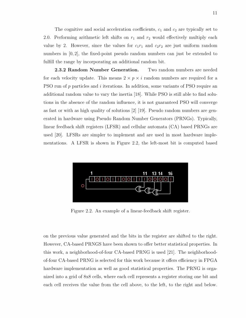
2.3.2 Random Number Generation. Two random numbers are needed

for each velocity update. This means 2 × p × i random numbers are required for a

PSO run of p particles and i iterations. In addition, some variants of PSO require an

additional random value to vary the inertia [18]. While PSO is still able to find solu-

tions in the absence of the random influence, it is not guaranteed PSO will converge

as fast or with as high quality of solutions [2] [19]. Pseudo random numbers are gen-

erated in hardware using Pseudo Random Number Generators (PRNGs). Typically,

linear feedback shift registers (LFSR) and cellular automata (CA) based PRNGs are

used [20]. LFSRs are simpler to implement and are used in most hardware imple-

mentations. A LFSR is shown in Figure 2.2, the left-most bit is computed based

Figure 2.2. An example of a linear-feedback shift register.

on the previous value generated and the bits in the register are shifted to the right.

However, CA-based PRNGS have been shown to offer better statistical properties. In

this work, a neighborhood-of-four CA-based PRNG is used [21]. The neighborhood-

of-four CA-based PRNG is selected for this work because it offers efficiency in FPGA

hardware implementation as well as good statistical properties. The PRNG is orga-

nized into a grid of 8x8 cells, where each cell represents a register storing one bit and

each cell receives the value from the cell above, to the left, to the right and below.

12

The 8x8 PRNG structure is shown in Figure 2.3. The new value of each cell is found

using a 4-input LUT, which is shown in Table 2.1. This implementation is efficient for

FPGA implementation because the FPGA utilized in this work, the Xilinx Virtex-II

Pro, uses 4-input LUTs to implement logic functions. Therefore, implementing the

neighborhood-of-four CA-based PRNG only requires one LUT and D-type flip-flop

per PRNG bit. To extract the generated number from the PRNG, the bit of each cell

is concatenated together into a bit-string. As there are 64 cells, the PRNG produces

a pseudorandom 64-bit string each cycle.

Figure 2.3. The structure of the neighborhood-of-four PRNG.

2.3.3 Control Module. The control module is used to initialize the

memory and generate the control signals for the modules. Upon reset the control

module enters an Init state which is used to initialize the counters to their respective

starting states. The control module then enters an Init-PRNG state to initialize the

13

Table 2.1. The values for the LUT in each PRNG cell.

x0x1x2x3 f0000 00001 10010 10011 10100 00101 00110 10111 01000 11001 11010 01011 11100 11101 01110 01111 0

PRNG. The Init-Particles state cycles through the particles and sets each particles

initial position, velocity and pbest position to a random value from the PRNG. The

gbest position is initialized in the same manner. The next state, Init-Pipeline is used

to prepare the module inputs. The Execute state is responsible for shifting each

particle through the pipeline and properly passing the modules the correct particles

information from memory while storing each particles new values as they are updated.

Upon either reaching a defined fitness or number of iterations, the Halt state is entered

and execution halts. The hardware PSO flowchart is shown in Figure 2.4.

2.4 RESULTS

All of the modules in the hardware PSO design have been designed in VHDL.

The hardware PSO design has been simulated and implemented on the Xilinx Virtex-

II Pro development platform [22]. In order to assess the performance of the hardware

PSO implementation, the hardware implementation is compared to a software im-

plementation developed in Matlab. The Matlab PSO implementation is executed on

14

Figure 2.4. The hardware PSO execution flowchart.

a 2.16 GHz Intel Core 2 Duo-based PC with 4 GB RAM. First, the performance

of the two implementations is compared with respect to the lowest fitness that the

implementation of able to achieve for the benchmark problems. Then the execution

speed of the two implementations is compared. Finally, the logic requirements for the

hardware implementation are discussed.

Two well-known benchmark optimization problems [23] have been selected for

comparing the two implementations. The first benchmark problem is the sphere

function:

f(x) =n�

i=1

x2i

(2.5)

The second benchmark problem is the Rosenbrock function:

f(x) =n−1�

i=1

100(xi+1 − x2i)2 + (xi − 1)2 (2.6)

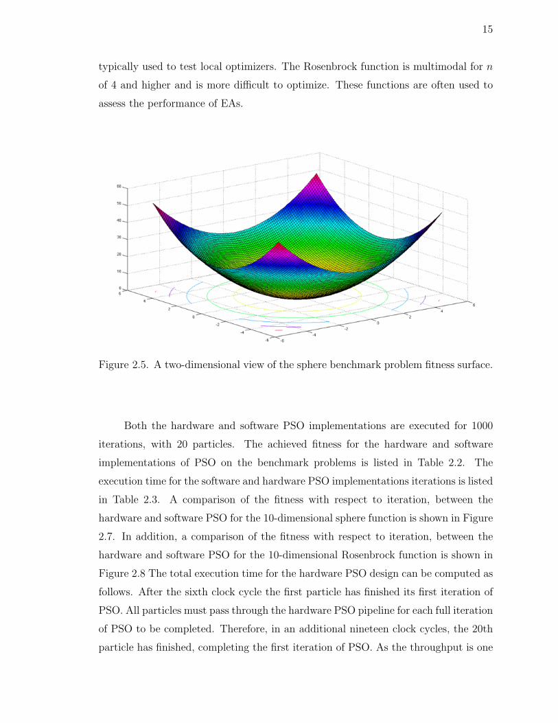
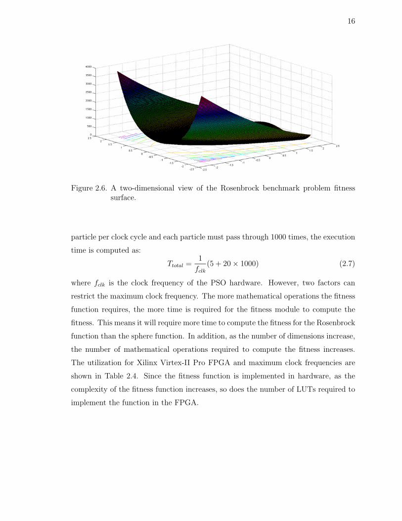
The surface of the sphere and Rosenbrock fitness functions are shown in Figures

2.5 and 2.6, respectively. The sphere function is a simple unimodal function that is

15

typically used to test local optimizers. The Rosenbrock function is multimodal for n

of 4 and higher and is more difficult to optimize. These functions are often used to

assess the performance of EAs.

Figure 2.5. A two-dimensional view of the sphere benchmark problem fitness surface.

Both the hardware and software PSO implementations are executed for 1000

iterations, with 20 particles. The achieved fitness for the hardware and software

implementations of PSO on the benchmark problems is listed in Table 2.2. The

execution time for the software and hardware PSO implementations iterations is listed

in Table 2.3. A comparison of the fitness with respect to iteration, between the

hardware and software PSO for the 10-dimensional sphere function is shown in Figure

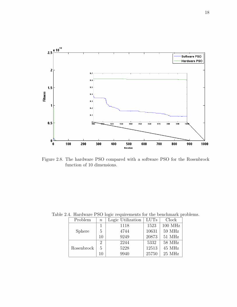
2.7. In addition, a comparison of the fitness with respect to iteration, between the

hardware and software PSO for the 10-dimensional Rosenbrock function is shown in

Figure 2.8 The total execution time for the hardware PSO design can be computed as

follows. After the sixth clock cycle the first particle has finished its first iteration of

PSO. All particles must pass through the hardware PSO pipeline for each full iteration

of PSO to be completed. Therefore, in an additional nineteen clock cycles, the 20th

particle has finished, completing the first iteration of PSO. As the throughput is one

16

Figure 2.6. A two-dimensional view of the Rosenbrock benchmark problem fitnesssurface.

particle per clock cycle and each particle must pass through 1000 times, the execution

time is computed as:

Ttotal =1

fclk

(5 + 20× 1000) (2.7)

where fclk is the clock frequency of the PSO hardware. However, two factors can

restrict the maximum clock frequency. The more mathematical operations the fitness

function requires, the more time is required for the fitness module to compute the

fitness. This means it will require more time to compute the fitness for the Rosenbrock

function than the sphere function. In addition, as the number of dimensions increase,

the number of mathematical operations required to compute the fitness increases.

The utilization for Xilinx Virtex-II Pro FPGA and maximum clock frequencies are

shown in Table 2.4. Since the fitness function is implemented in hardware, as the

complexity of the fitness function increases, so does the number of LUTs required to

implement the function in the FPGA.

17

Table 2.2. Achieved fitness after 1000 iterations for benchmark problems.Problem n Software PSO Fitness Hardware PSO Fitness

Sphere1 0.00 0.005 0.00 0.0010 0.073 0.001

Rosenbrock2 0.00 0.005 0.044 0.08510 8.081 8.615

Table 2.3. Execution time for software and hardware PSO implementations.Problem n Software PSO Time Hardware PSO Time

Sphere1 2.07 sec. 200 µs5 5.79 sec. 338 µs10 10.99 sec. 392 µs

Rosenbrock2 2.14 sec. 344 µs5 5.95 sec. 444 µs10 10.91 sec. 800 µs

Figure 2.7. The hardware PSO compared with a software PSO for the sphere functionof 10 dimensions.

18

Figure 2.8. The hardware PSO compared with a software PSO for the Rosenbrockfunction of 10 dimensions.

Table 2.4. Hardware PSO logic requirements for the benchmark problems.Problem n Logic Utilization LUTs Clock

Sphere1 1118 1523 100 MHz5 4744 10631 59 MHz10 9249 20873 51 MHz

Rosenbrock2 2244 5332 58 MHz5 5228 12513 45 MHz10 9940 25750 25 MHz

19

3 IMPLEMENTATION OF NEURAL NETWORK

3.1 INTRODUCTION

NNs are universal function approximators. The structure of a multilayer per-

ceptron, which is used in this thesis work, is given in Figure 3.1. This network has

two inputs, three hidden neurons, and one output. The input and output layers are

linear, while the hidden layer uses the hyperbolic tangent function. The vector w

contains the weights for the input layer while the vector v contains the weights for

the hidden layer. The output of the network is computed as follows:

ai =nI�

j=1

wi,jxj,i,i = 1, ..., nH

di =eai − e−ai

eai + e−ai,i = 1, ..., nH

y =nH�

i=1

vidi

(3.1)

where nH and nI are the number of hidden neurons and inputs, respectively.

Figure 3.1. An NN with an input, hidden and output layer.

20

NNs are inherently parallel, with each layer of neurons processing incoming

data independently of each other. While general purpose processors have reached

impressive processing speeds, they still cannot fully exploit this inherent parallelism

due to their sequential architecture [24]. In order to achieve the high neural network

throughput need for real-time applications, a custom hardware design is needed.

There are different ways to exploit the parallelism of NNs in hardware. For

instance, each neuron in a given layer can be processed in parallel; this results in

one layer being processed at a given movement. As an alternative, each of the layers

could be processed simultaneously. In this design each of the neurons would be

processed simultaneously. In terms of performance, the latter would yield the greatest

throughput, however, logic resources on the FPGAs is limited. The most costly

operation in computing an NN output is multiplication, for an NN with I inputs, H

hidden neurons and O outputs, I × H + H × O multiplications are required. The

FPGA resources required for a single multiplication operation are dependent on the

width of the multiplication, i.e. a 8-bit by 8-bit multiplication or a 12-bit by 12-

bit multiplication. In addition to the resources required for the multiplications, the

activation function must be implemented on the FPGA. The activation function is

typically a non-linear function such as the hyperbolic tangent:

f(x) =ex − e−x

ex + e−x(3.2)

which requires two exponentials, ex and e−x to be computed. These operations would

also require a large amount of FPGA resources and computing them directly is usually

avoided as a result. An alternative is to compute a linear piece-wise approximation

and program it into the LUTs on the FPGA. Although the approximations will lose

some precision the LUTs can be accessed in a single clock cycle which is far faster

than computing the real solution, in addition to consuming far less FPGA resources.

3.2 DESIGN APPROACH

Although hardware implementations of NNs offer the best performance, soft-

ware implementations are far more common. As stated in Section 1, the hardware

implementations are more difficult to design. More importantly, its more difficult

21

for engineers without digital system design backgrounds to learn how to quickly de-

velop digital systems. Typically designing a digital system requires experience with

a hardware description language (HDL) such as VHDL or Verilog.

Xilinx System Generator is a software tool for modeling and designing FPGA-

based systems in MathWorks Simulink [25]. This tool presents a high level abstract

view of the whole system, yet automatically maps the system to a faithful hard-

ware implementation. System Generator allows hardware designers to design high-

performance, high-level DSP systems using custom Simulink blocks. Designers can

use the System Generator blocks to build a hardware system, simulate the system

using Simulink and produce a bit file which can then be programmed onto a FPGA.

Since Simulink is tightly integrated with MathWorks MATLAB, it becomes easier to

implement complex algorithms in hardware than purely using a HDL. Furthermore,

System Generator allows blocks designed using an HDL to be imported and simulated

within a system designed using System Generator.

As stated in Section 3.1, NNs require a large number of multiplications and the

multiplication operation is very resource consuming when implemented on a FPGA.

This places a constraint on the size of the neural network; even if LUTs are used

for activation computation, the FPGA must be able to provide two multipliers per

neuron. Due to this constraint, a multiplier-rich FPGA platform has been selected,

the Xilinx Virtex-II Pro Development System. The Virtex-II Pro boasts 136 18-bit

embedded multipliers, two embedded PowerPC processors and 30,000 programmable

logic cells [22]. The Virtex-II is targeted at high-performance DSP and research

applications and is well suited for a FPGA-based NN implementation.

3.3 NN HARDWARE IMPLEMENTATION

The following sections discuss the design of the FPGA-based NN.

3.3.1 Implementing the Neuron MAC. The neurons are the essential

components of NNs. In a feedforward NN, each neuron receives the output of each

neuron in the preceding layer. The neuron model is shown in Figure 3.2. The activata-

tion of a neuron is the sum of the neurons inputs multiplied by their corresponding

22

weights:

a =N�

i=0

xi · wi (3.3)

where xi is the output of the ith neuron in the preceding layer and wi is the cor-

responding weight. This is known as performing a Multiply ACcumulate (MAC)

operation. Each neuron has an activation function, such as the hyperbolic tangent

function. The output of the neuron is found by applying the activation function to

the activation of the neuron.

Figure 3.2. A diagram of the neuron model.

The MAC operation is modeled using a multiply and accumulate block. The

MAC subsystem is provided an input x, the corresponding weight w and a reset

signal. The reset signal is used to reset the accumulator to 0 when all the pairs of

inputs and weights have been processed. The MAC subsystem is illustrated in Figure

3.3.

Figure 3.3. MAC hardware subsystem.

23

3.3.2 Implementing the Activation Function LUT. As discussed in

Section 3.1, the activation function is approximated using a LUT-Based Activation

Function (LUTAF) module. The activation functions need to be approximated, using

a simple linear function:

f(x) = α2 + c2 ∗ x (3.4)

where x is the activation of the neuron and α1 and α2 are LUT constants. To solve

for the constants, the interval over which the approximations will hold must be de-

termined. In this thesis, the interval was selected to be x ∈ [−8, 7]. The number of

linearized intervals also needs to be determined (as a power of two). In this thesis,

the number of subintervals was selected to be 24 = 16. The linearized regions can be

found in Table 3.1. Now, the values for α1 and α2 must be computed for the given

activation function, the approximated interval and the respective number of subinter-

vals. In this thesis the hyperbolic tangent activation function was used. Therefore,

to compute α1 and α2 for a given region the following system must be solved:

α1 + α2 ∗ L =eU − e−U

eU + e−U(3.5)

α1 + α2 ∗ U =eL − e−L

eL + e−L(3.6)

where L is lower boundary in the subinterval and U is the upper boundary in the

subinterval. Solving for α1 and α2 using Matlab’s Symbolic Math toolbox results in:

α1 =L ∗ eU − U ∗ eU − U ∗ eU ∗ eL + L ∗ eU ∗ eL + U + eL ∗ L− L + U ∗ eL

−U − U ∗ eU − U ∗ eL − U ∗ eU ∗ eL + L + L ∗ eU + eL ∗ L + L ∗ eU ∗ eL

(3.7)

α2 =2 ∗ (eU − eL)

−U − U ∗ eU − U ∗ eL − U ∗ eU ∗ eL + L + L ∗ eU + eL ∗ L + L ∗ eU ∗ eL

(3.8)

where eU and eL are constants which equal e−2∗U and e−2∗L, respectively. The values

for α1 and α2 are now computed for each subinterval using these solutions. The

resulting values for this work can be found in Table 3.1. The resulting approximation

is shown in Figure 3.4.

24

Table 3.1. The values for the hyperbolic tangent activation Function LUT where x ∈[L, U ].

L U α1 α2

6 7 0.99992 1.0625e-005

5 6 0.99952 7.8507e-005

4 5 0.99701 0.0005799

3 4 0.98223 0.0042745

2 3 0.90197 0.031027

1 2 0.55916 0.20243

0 1 -2.2204e-016 0.76159

-1 0 0 0.76159

-2 -1 -0.55916 0.20243

-3 -2 -0.90197 0.031027

-4 -3 -0.98223 0.0042745

-5 -4 -0.99701 0.0005799

-6 -5 -0.99952 7.8507e-005

-7 -6 -0.99992 1.0625e-005

-8 -7 -0.99999 1.438e-006

The hardware implementation of the LUTAF is constructed from three main

elements, the memory element which contains the linearized constants α1 and α2, a

multiplier and an addition unit. The LUTAF subsystem can be found in Figure 3.5.

The proper subinterval is determined by selecting the upper k most significant bits

of the input, x, where 2k is the number of subintervals. The upper k bits are used

to index the corresponding values of α1 and α2 by using the k bits as the address to

the memory elements. The values for α2 and x are passed to a multiplier while α1 is

latched (delayed to match the propagation of the signal (α2× x)). Finally, the terms

(α2) and (α2 × x) are added to produce the activation function approximation.

3.3.3 Implementing the Complete Hardware Neuron. The hardware

neuron is a combination of the Neuron MAC (Section 3.3.1) and the LUTAF (Section

3.3.2) and a memory element to store the weights. The complete hardware neuron

25

Figure 3.4. LUTAF approximation.

Figure 3.5. LUTAF approximation subsystem.

subsystem can be seen in Figure 3.6. The hardware neuron receives the values x,

w addr, reset and latch f. The input x is the value of the current input being processed

(i.e. from the preceding neuron i). The value of w addr is the index of the current

input being processed, i. This signal is used to index the value of the corresponding

weight in the memory element. The reset signal is used to reset the MAC as explained

26

in Section 3.3.1. The latch f signal is used to indicate when the output of the MAC

is valid and should be latched (since the MAC sequentially accumulates values, the

values other than the last are incomplete sums). The latch my latch is responsible

for latching the result of the MAC when its valid, based on the latch f signal. The

latched output from the MAC is connected to the input to the LUTAF subsystem

which computes the approximated activation function output.

Figure 3.6. The complete hardware neuron.

3.3.4 Implementing the NN Layer Control Block. As the hardware

neurons process the input/weight pairs sequentially, a mechanism is needed to cycle

through each of the outputs from the previous layer and provide them to the hardware

neurons in the respective current layer. The LCB (Layer Control Block) receives the

outputs from the neurons in the previous layer as well as a global reset signal. The

LCB is responsible for providing the value of the current input being processed,

the index of the current input, the MAC reset and latch f signals to the hardware

neurons. Since the hardware neurons process each input/weight pair in parallel, each

hardware neuron receives the same signals. The LCB is implemented as a finite state

machine. The finite state machine for a layer receiving two inputs with three neurons

is illustrated in Figure 3.7, while the LCB and hardware neurons are shown in Figure

3.8. The operation of a hardware neuron being controlled by a LCB can be seen in

Figure 3.9.

27

Figure 3.7. The LCB finite state machine (2× 3 Layer).

3.3.5 Implementing a Three-Layer NN. Using the components developed

in Sections 3.3.3 and 3.3.4, an NN of arbitrary size can be constructed. The LCB

finite state machines must have the corresponding states for the layers inputs and

outputs. For a NN of size 1 × 3 × 1 (a bias is included in each layer), the hardware

NN is illustrated in Figure 3.10. The inputs to the FPGA-Based NN are the global

reset signal, ResetSeq which synchronize the two LCBs and the x1 signal which is the

input the NN. The FPGA-Based NN produces the signal F which is the output of the

NN. The Gate In and Gateway Out blocks indicate ports on the FPGA where external

28

Figure 3.8. A LCB controlling three hardware neurons (2× 3 Layer).

signals are presented to the FPGA and received from the FPGA, respectively. The

Gateway blocks are configured to specify specific I/O pins on the FPGA.

To construct a n-layer NN, (n− 1) LCBs are required; the input layer does not

require a LCB, only layers which contain neurons that receive input from multiple

sources require a LCB. The number of neurons in each layer impact the number of the

hardware resources consumed as well as the throughput of the NN. Layers that do not

require a non-linear transfer function (linear layers) require less hardware resources

to implement because there is no need for each neuron to have a LUTAF module.

Therefore, a non-linear n-neuron hidden layer would require more hardware resources

than a n-neuron linear output layer. The number of input patterns processed in a

given time is strictly a function of the largest layer in the NN. In other words, a

1× 10× 1 NN will process the same number of input patterns as a 5× 10× 5 NN in a

given amount of time. This is due to the fact that the LCBs must operate together,

each must process the first input at the same time, one cannot begin processing a

new input pattern before the other LCBs are finished for all other layers.

29

Figure 3.9. A hardware neuron being controlled by a LCB.

Figure 3.10. A FPGA-based NN (of size 1× 3× 1).

30

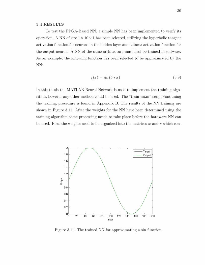
3.4 RESULTS

To test the FPGA-Based NN, a simple NN has been implemented to verify its

operation. A NN of size 1× 10× 1 has been selected, utilizing the hyperbolic tangent

activation function for neurons in the hidden layer and a linear activation function for

the output neuron. A NN of the same architecture must first be trained in software.

As an example, the following function has been selected to be approximated by the

NN:

f(x) = sin (5 ∗ x) (3.9)

In this thesis the MATLAB Neural Network is used to implement the training algo-

rithm, however any other method could be used. The “train nn.m” script containing

the training procedure is found in Appendix B. The results of the NN training are

shown in Figure 3.11. After the weights for the NN have been determined using the

training algorithm some processing needs to take place before the hardware NN can

be used. First the weights need to be organized into the matrices w and v which con-

Figure 3.11. The trained NN for approximating a sin function.

31

tain the weights for the hidden and output layers, respectively. The Xilinx System

Generator Single Port Read-Only Memory (ROM) is used in each hardware neuron

to store its respective weights. The ROM in each neuron is configured to select the

correct weight indices from the trained weights in the MATLAB workspace (from

matrices w and v), each neuron only stores the weights it needs to compute its own

output. Here the weights are converted into 18.12 fixed-point1 representation when

they are loaded into the ROMs.

In the second part of this process the values for the LUTAF must be loaded

into each Neurons LUTAF ROM. A MATLAB script it used to solve for the values of

α1 and α2 using the method described in Section 3.4. In order for LUTAF constants

α1 and α2 to be used by the FPGA-Based NN, the values of the constants found in

MATLAB must also be converted into 18.12 fixed-point.

Finally, the input patterns that were used for training are processed using a

MATLAB script for presentation to the Xilinx System Generator Gateway In port,

NN Input. In addition, a reset signal is prepared in the same manner for the Gateway

In port NN Reset. These steps are performed by the script “nn load.m” in Appendix

B.

Now that the The FPGA-based NN model has of the necessary values converted

and loaded, it can be simulated. The output of the Simulink simulation can be found

in Figure 3.12. However, the output is in terms of clock cycles. In order to compare

the hardware NN output against the software NN output, the software NN output

must be upsampled. This is performed by the script “test nn model.m”, in Appendix

B. The output of each hardware hidden neuron is compared with the software hidden

neurons in Figure 3.13. The output of the first five hidden neurons are shown in

Figure 3.13(a) while the output of the last five hidden neurons are shown in Figure

3.13(b). The output of the hardware NN is compared against the software NN in

Figure 3.14. The simulations presented are not high-level simulations, they are cycle-

accurate simulations of the synthesized hardware NN design executing on the Xilinx

Virtex-II Pro FPGA platform.

118.12 fixed-point representation indicates that a total of 18 bits are used and 12 of the bits arededicated to the fractional portion of the value, leaving 6 bits for the integer portion of the value.

32

Figure 3.12. The output of the Simulink simulation of the FPGA-based NN.

The design is then synthesized using Xilinx ISE. The FPGA resources used can

be found in Figure 3.15. It should be noted that the 1x10x1 hardware NN only

requires approximately 6% of the Xilinx Virtex II Pro’s logic resources. The critical

path has a delay of 15.4 ns, resulting in a maximum clock rate of 64 MHz. Using a

newer FPGA, such as the Xilinx Virtex-4 or Xilinx Virtex-5 will result in even higher

clock rates. The logic utilization will vary if another FPGA is used, depending on

the size of the FPGA being targeted.

33

(a) The output of hidden neurons 1-5.

(b) The output of hidden neurons 6-10.

Figure 3.13. Comparing the output of hidden neurons of the FPGA-based NN andMatlab-based NN.

34

Figure 3.14. Comparing the output of the FPGA-based NN and Matlab-based NN.

Figure 3.15. The hardware resources used for the 1×10×1 NN on the Xilinx Virtex-IIPro FPGA.

35

4 CONCLUSIONS AND FUTURE WORK

This thesis has presented two independent hardware designs, a hardware imple-

mentation of the PSO algorithm and a hardware implementation of an NN.

A pipelined hardware implementation of PSO has been presented. The hard-

ware PSO design implemented on a Xilinx Virtex-II Pro FPGA is shown to perform

well on two standard benchmark problems when compared to a common software

implementation of PSO in Matlab. When compared to the software implementation,

the hardware implementation is between 6,220 - 28,935 times faster. The system is

targeted for real-time applications where minimizing PSO execution time is critical.

One such application is real-time neural network training.

A high-performance Xilinx Virtex-II Pro FPGA-based NN architecture has been

presented. The system allows feed-forward NNs to be implemented on FPGAs re-

sulting in very high throughput. The hardware NN is developed using a model-based

methodology which is easier for researchers who are not knowledgeable in a HDL to

modify for their specific application.

The PSO hardware design in this thesis did not utilize any explicit memory

such as RAM for storing the PSO variables2; instead, all of the variables were simply

stored in registers. This approach is not the most efficient for problems which have

fitness function with a large number of dimensions. Training a large NN would be

such a case, where the number of weights could be in the hundreds or thousands. For

these applications, the PSO hardware design presented could be augmented with a

memory interface that used a RAM module to store PSO variables.

The hardware NN presented in this thesis was of the feed-forward architecture.

None of the outputs or outputs from the hidden layer were passed back as inputs

to the NN. These recurrent architectures have been shown to offer more capabilities

for approximating problems with temporally related data. The hardware NN design

presented here could be extended to incorporate recurrent architectures by modifying

the LCBs.

2While FPGAs utilize memory components as LUTs to implement logic functions, they also havea number of block RAMs available that are more area-efficient for storing large amounts of data.

APPENDIX A

HARDWARE PSO SOURCE CODE

37

The main portions of the VHDL source code developed for the hardware PSO

implementation has been selected for inclusion in this appendix for reference. All of

the VHDL source code was compiled and simulated using Mentor Graphics ModelSim

6.5. The source code was synthesized using Xilinx ISE 10.1.

38

PSO.vhd

1 l ibrary IEEE ;

2 use IEEE . STD LOGIC 1164 .ALL;

3 use IEEE .STD LOGIC ARITH.ALL;

4 use IEEE .STD LOGIC UNSIGNED.ALL;

5

6 LIBRARY i e e e p ropo s ed ;

7 USE i e e e p ropo s ed . math ut i l i t y pkg .ALL;

8 USE i e e e p ropo s ed . f i x ed pkg .ALL;

9

10 USE WORK. pso package .ALL;

11

12 −−−− Uncomment the f o l l ow i n g l i b r a r y d e c l a r a t i on i f i n s t a n t i a t i n g

13 −−−− any Xi l i n x p r im i t i v e s in t h i s code .

14 −− l i b r a r y UNISIM;

15 −−use UNISIM. VComponents . a l l ;

16

17 entity PSO i s

18 PORT(

19 SYSTEM CLK : in s t d l o g i c ;

20 SWITCHES : in STD LOGIC VECTOR(1 downto 0) ;

21 LEDS : out STD LOGIC VECTOR(1 downto 0) ;

22 GBEST : out STD LOGIC VECTOR(7 downto 0)

23 ) ;

24 end PSO;

25

26 architecture Behaviora l of PSO i s

27

28 signal DCM IBUFG OUT, DCM CLK0 OUT, DCMLOCKED : s t d l o g i c ;

29 signal c l k : s t d l o g i c ;

30 signal gb e s t p o s i t i o n : t o t a l p o s i t i o n ;

31 signal g b e s t f i t n e s s : s f i x e d (FITNESS BITS LEFT downto −FITNESS BITS RIGHT) ;

32 signal PSO reset , PSO fin ished : s t d l o g i c ;

33 signal i t e r a t i o n : unsigned (ITERATION COUNT BITS−1 downto 0) ;

34

35 signal gb e s t f i t n e s s tmp : s t d l o g i c v e c t o r (FITNESS BITS LEFT +

FITNESS BITS RIGHT downto 0) ;

39

36

37 COMPONENT dcm0

38 PORT(

39 CLKIN IN : IN s t d l o g i c ;

40 CLKDV OUT : OUT s t d l o g i c ;

41 CLKIN IBUFG OUT : OUT s t d l o g i c ;

42 CLK0 OUT : OUT s t d l o g i c ;

43 LOCKED OUT : OUT s t d l o g i c

44 ) ;

45 ENDCOMPONENT;

46

47 COMPONENT pso top

48 PORT (

49 clk , r e s e t : in s t d l o g i c ;

50 gbest : t o t a l p o s i t i o n ;

51 gbe s t e : out s f i x e d (FITNESS BITS LEFT downto −FITNESS BITS RIGHT) ;

52 i t e r a t i o n : out unsigned (ITERATION COUNT BITS−1 downto 0) ;

53 f i n i s h e d : out s t d l o g i c ) ;

54 ENDCOMPONENT;

55

56 begin

57

58 Inst dcm0 : dcm0 PORTMAP(

59 CLKIN IN => SYSTEM CLK,

60 CLKDV OUT => c lk ,

61 CLKIN IBUFG OUT => DCM IBUFG OUT,

62 CLK0 OUT => DCM CLK0 OUT,

63 LOCKED OUT => DCMLOCKED

64 ) ;

65

66 In s t p s o t op0 : pso top PORTMAP(

67 c l k => c lk ,

68 r e s e t => PSO reset ,

69 gbest => gbe s t po s i t i on ,

70 gbe s t e => g b e s t f i t n e s s ,

71 i t e r a t i o n => i t e r a t i o n ,

72 f i n i s h e d => PSO finished

73 ) ;

74

40

75 PSO reset <= SWITCHES(0) ;

76

77 LEDS(0) <= NOT PSO reset ;

78 LEDS(1) <= NOT PSO finished ;

79

80 gb e s t f i t n e s s tmp <= t o s l v ( g b e s t f i t n e s s ) ;

81

82 −−GBEST <= g b e s t p o s i t i o n (7 downto 0) ;

83 GBEST <= gbe s t f i t n e s s tmp (7 downto 0) ;

84

85 end Behaviora l ;

41

pso_package.vhd

1 −−LIBRARY f l o a t f i x l i b ;

2 −−USE f l o a t f i x l i b . ma t h u t i l i t y p k g .ALL;

3 −−USE f l o a t f i x l i b . f i x e d p k g .ALL;

4




8

9 PACKAGE pso package i s

10 constant NUM PARTICLES : natura l := 20 ;

11 constant RN BITS : natura l := 64 ;

12 constant NUM DIMENSIONS : natura l := 10 ;

13

14 constant POSITION BITS LEFT : natura l := 7 ;

15 constant POSITION BITS RIGHT : natura l := 9 ;

16

17 −−cons tant FITNESS BITS LEFT : na tura l := POSITION BITS LEFT;

18 −−cons tant FITNESS BITS RIGHT : na tura l := POSITION BITS RIGHT;

19 −−cons tant FITNESS BITS LEFT : na tura l := POSITION BITS LEFT +

POSITION BITS LEFT + NUM DIMENSIONS;

20 −−cons tant FITNESS BITS RIGHT : na tura l := POSITION BITS RIGHT +

POSITION BITS RIGHT;

21 constant FITNESS BITS LEFT : natura l := 43+NUM DIMENSIONS + 6 ;

22 constant FITNESS BITS RIGHT : natura l := 36 ;

23

24 constant C BITS LEFT : natura l := 2 ;

25 constant C BITS RIGHT : natura l := 2 ;

26

27 constant R BITS LEFT : natura l := 0 ;

28 constant R BITS RIGHT : natura l := 9 ;

29

30 constant W BITS LEFT : natura l := 0 ;

31 constant W BITS RIGHT : natura l := 3 ;

32

33 −−cons tant VELOCITY BITS LEFT : na tura l := POSITION BITS LEFT+1+

R BITS LEFT+C BITS LEFT+2;

42

34 −−cons tant VELOCITY BITS RIGHT : na tura l := POSITION BITS RIGHT+

R BITS RIGHT+C BITS RIGHT;

35 constant VELOCITY BITS LEFT : natura l := POSITION BITS LEFT ;

36 constant VELOCITY BITS RIGHT : natura l := POSITION BITS RIGHT+1;

37

38 constant PARTICLE COUNT BITS : natura l := 5 ;

39 constant DIMENSION COUNT BITS : natura l := 4 ;

40

41 constant ITERATION COUNT BITS : natura l := 10 ;

42 constant MAX ITERATIONS : natura l := 1000 ;

43

44 type t o t a l p o s i t i o n i s array (0 to NUM DIMENSIONS−1) of s f i x e d (

POSITION BITS LEFT downto −POSITION BITS RIGHT) ;

45 type t o t a l v e l o c i t y i s array (0 to NUM DIMENSIONS−1) of s f i x e d (

VELOCITY BITS LEFT downto −VELOCITY BITS RIGHT) ;

46

47 END pso package ;

43

pso_top.vhd


2 LIBRARY IEEE ;

3 USE IEEE . s t d l o g i c 1 1 6 4 .ALL;

4 USE IEEE . numer ic std .ALL;

5




9




13

14 ENTITY pso top IS

15 PORT ( c lk , r e s e t : in s t d l o g i c ;

16 gbest : out t o t a l p o s i t i o n ;

17 gbe s t e : out s f i x e d (FITNESS BITS LEFT downto −FITNESS BITS RIGHT) ;

18 i t e r a t i o n : out unsigned (ITERATION COUNT BITS−1 downto 0) ;

19 f i n i s h e d : out s t d l o g i c ) ;

20 END ENTITY pso top ;

21

22 ARCHITECTURE behav io ra l OF pso top IS

23

24 −− Reset S i gna l s

25 signal r e s e t modu le s : s t d l o g i c ;

26 −− S i gna l s to RNG

27 signal r e s e t rng , rng enab l e : s t d l o g i c ;

28 −− S i gna l s from RNG

29 signal rn : s t d l o g i c v e c t o r (RN BITS−1 downto 0) ;

30 −− S i gna l s to F i tne s s module

31 signal p o s i t i o n t o e v a l : t o t a l p o s i t i o n ;

32 −− S i gna l s from Fi tne s s module to Best modules

33 signal f i t n e s s f r om e v a l : s f i x e d (FITNESS BITS LEFT downto −FITNESS BITS RIGHT) ;

34 −− S i gna l s to Best modules

35 signal p o s i t i o n t o b e s t : t o t a l p o s i t i o n ;

44

36 signal pbe s t po s i t i on , g b e s t p o s i t i o n : t o t a l p o s i t i o n ;

37 signal pb e s t f i t n e s s , g b e s t f i t n e s s : s f i x e d (FITNESS BITS LEFT

downto −FITNESS BITS RIGHT) ;

38 −− S i gna l s from Best modules

39 signal new pbes t pos i t i on , n ew gbe s t po s i t i on : t o t a l p o s i t i o n ;

40 signal new pbe s t f i t n e s s , n ew gb e s t f i t n e s s : s f i x e d (

FITNESS BITS LEFT downto −FITNESS BITS RIGHT) ;

41 −− S i gna l s to Update Ve l o c i t y module

42 signal v e l o c i t y t o upd a t e v e l o c i t y : t o t a l v e l o c i t y ;

43 signal po s i t i o n t o upda t e v e l o c i t y : t o t a l p o s i t i o n ;

44 signal rn1 , rn2 : s f i x e d (R BITS LEFT−1 downto −R BITS RIGHT) ;

45 −− S i gna l s to Update Pos i t i on module

46 signal new ve loc i ty : t o t a l v e l o c i t y ;

47

48 −− S i gna l s from Update Pps i t i on module

49 signal new pos i t i on : t o t a l p o s i t i o n ;

50

51 −− Par t i c l e Memory

52 type par t i c l e po s i t i on mem i s array (0 to NUM PARTICLES−1) of

t o t a l p o s i t i o n ;

53 type pa r t i c l e v e l o c i t y mem i s array (0 to NUM PARTICLES−1) of

t o t a l v e l o c i t y ;

54 type pa r t i c l e f i t n e s s mem i s array (0 to NUM PARTICLES−1) of s f i x e d (

FITNESS BITS LEFT downto −FITNESS BITS RIGHT) ;

55

56 signal position mem : pa r t i c l e po s i t i on mem ;

57 signal velocity mem : pa r t i c l e v e l o c i t y mem ;

58 signal pbest pos i t ion mem : pa r t i c l e po s i t i on mem ;

59 signal pbes t f i tne s s mem : pa r t i c l e f i t n e s s mem ;

60 signal gbest pos i t ion mem : t o t a l p o s i t i o n ;

61 signal gbes t f i tne s s mem : s f i x e d (FITNESS BITS LEFT downto −FITNESS BITS RIGHT) ;

62 signal i n i t f i t n e s s t o : s f i x e d (FITNESS BITS LEFT downto −FITNESS BITS RIGHT) ;

63

64 −− PSO Top FSM

65 TYPE s t a t e s IS ( i d l e , i n i t r n g , i n i t p a r t i c l e s 1 , i n i t p a r t i c l e s 2 ,

i n i t p a r t i c l e s 3 , i n i t p i p e l i n e 1 , i n i t p i p e l i n e 2 , exec , done ) ;

66 signal s t a t e : s t a t e s ;

45

67 signal dimens ion cnt : unsigned (DIMENSION COUNT BITS−1 downto 0) ;

68 signal p a r t i c l e c n t i n i t : unsigned (PARTICLE COUNT BITS−1 downto 0) ;

69 signal p a r t i c l e c n t s t a g e 1 : unsigned (PARTICLE COUNT BITS−1 downto

0) ;


0) ;


0) ;


0) ;


0) ;

74 signal i t e r a t i o n c n t : unsigned (ITERATION COUNT BITS−1 downto 0) ;

75 signal i n i t r n g c n t : unsigned (4 downto 0) ;

76 BEGIN

77 rng : ENTITY work . RandomNumberGenerator ( General )

78 PORTMAP ( c lk , rng enable , r e s e t rng , rn ) ;

79

80 d e l a y p o s i t i o n s : for i in 0 to NUM DIMENSIONS−1 generate

81 d e l a y po s i t i o n 1 : ENTITY work . d e l a y po s i t i o n ( behav io ra l )

82 PORTMAP ( c lk , p o s i t i o n t o e v a l ( i ) , p o s i t i o n t o b e s t ( i ) ) ;

83 d e l a y po s i t i o n 2 : ENTITY work . d e l a y po s i t i o n ( behav io ra l )

84 PORTMAP ( c lk , p o s i t i o n t o b e s t ( i ) , p o s i t i o n t o upda t e v e l o c i t y (

i ) ) ;

85 end generate d e l a y p o s i t i o n s ;

86

87 −− f i t n e s s e v a l : ENTITY work . f i tness dummy ( b ehav i o r a l )

88 −− PORT MAP ( c lk , p o s i t i o n t o e v a l , f i t n e s s f r om e v a l ) ;

89 −− f i t n e s s e v a l : ENTITY work . f i t n e s s s q u a r e d ( b eha v i o r a l )

90 −− PORT MAP ( c lk , p o s i t i o n t o e v a l , f i t n e s s f r om e v a l ) ;

91 f i t n e s s e v a l : ENTITY work . f i t n e s s r o s e nb r o c k ( behav io ra l )

92 PORTMAP ( c lk , p o s i t i o n t o e v a l , f i t n e s s f r om e v a l ) ;

93

94 update pbest : ENTITY work . update best ( behav io ra l )

95 PORTMAP ( c lk , re se t modules , p o s i t i o n t o b e s t , f i t n e s s f r om eva l ,

pbe s t po s i t i on , p b e s t f i t n e s s ,

96 new pbes t pos i t i on , n ew pbe s t f i t n e s s ) ;

97

98 update gbest : ENTITY work . update best ( behav io ra l )

46

99 PORTMAP ( c lk , re se t modules , p o s i t i o n t o b e s t , f i t n e s s f r om eva l ,

new gbes t pos i t i on , n ew gbe s t f i t n e s s ,

100 new gbes t pos i t i on , n ew gb e s t f i t n e s s ) ;

101

102 pso d imens ions : for i in 0 to NUM DIMENSIONS−1 generate

103 pso dimens ion : ENTITY work . pso dimens ion ( behav io ra l )

104 PORTMAP ( c lk , re se t modules , p o s i t i o n t o upda t e v e l o c i t y ( i ) ,

v e l o c i t y t o upd a t e v e l o c i t y ( i ) , n ew pbe s t po s i t i on ( i ) ,

n ew gbe s t po s i t i on ( i ) ,

105 rn1 , rn2 , new ve loc i ty ( i ) , new pos i t i on ( i )

106 ) ;

107 end generate pso dimens ions ;

108

109 i t e r a t i o n <= i t e r a t i o n c n t ;

110

111 PSO main : PROCESS( c lk , r e s e t )

112 BEGIN

113 −− Go in to ’ i d l e ’ s t a t e upon r e s e t

114 IF r e s e t = ’1 ’ THEN

115 s t a t e <= i d l e ;

116 −− Reset modules

117 re s e t modu le s <= ’1 ’ ;

118 −− Reset RNG

119 r e s e t r n g <= ’1 ’ ;

120 rng enab l e <= ’0 ’ ;

121 f i n i s h e d <= ’0 ’ ;

122 i t e r a t i o n c n t <= ( others => ’ 0 ’ ) ;

123 ELSIF ( c lk ’EVENT AND c l k = ’1 ’) THEN

124 CASE s t a t e IS

125 WHEN i d l e => −− Was r e s e t

126 s t a t e <= i n i t r n g ;

127 p a r t i c l e c n t i n i t <= ( others => ’ 0 ’ ) ;

128 dimens ion cnt <= ( others => ’ 0 ’ ) ;

129 i t e r a t i o n c n t <= ( others => ’ 0 ’ ) ;

130 f i n i s h e d <= ’0 ’ ;

131 −−Maximum ( worst ) f i t n e s s va lue

132 i n i t f i t n e s s t o <= (FITNESS BITS LEFT => ’ 0 ’ , others => ’ 1 ’ )

;

133 i n i t r n g c n t <= ( others => ’ 0 ’ ) ;

47

134

135 p a r t i c l e c n t s t a g e 1 <= ( others => ’ 0 ’ ) ;

136 p a r t i c l e c n t s t a g e 2 <= to uns igned (NUM PARTICLES−2,

PARTICLE COUNT BITS) ;







140

141 WHEN i n i t r n g => −− Cycle through some RNG va lue s so

they are ’more random ’

142 r e s e t r n g <= ’0 ’ ;

143 rng enab l e <= ’1 ’ ;

144 i f ( i n i t r n g c n t < ”11111” ) then

145 i n i t r n g c n t <= i n i t r n g c n t + 1 ;

146 else

147 s t a t e <= i n i t p a r t i c l e s 1 ;

148 end i f ;

149 WHEN i n i t p a r t i c l e s 1 => −− I n i t a l i z e a l l p a r t i c l e

memory to random va lue s

150 position mem ( t o i n t e g e r ( p a r t i c l e c n t i n i t ) ) ( t o i n t e g e r (

d imens ion cnt ) ) <= t o s f i x e d ( rn (POSITION BITS LEFT +

POSITION BITS RIGHT downto 0) , POSITION BITS LEFT , −POSITION BITS RIGHT) ;

151 velocity mem ( t o i n t e g e r ( p a r t i c l e c n t i n i t ) ) ( t o i n t e g e r (

d imens ion cnt ) ) <= t o s f i x e d (0 , VELOCITY BITS LEFT, −VELOCITY BITS RIGHT) ;

152

153 i f ( d imens ion cnt < NUM DIMENSIONS−1) then

154 dimens ion cnt <= dimens ion cnt + 1 ;

155 else


157 i f ( p a r t i c l e c n t i n i t < NUM PARTICLES−1) then

158 p a r t i c l e c n t i n i t <= p a r t i c l e c n t i n i t + 1 ;

159 else



48

162 end i f ;

163 end i f ;

164



166 −−pbes t pos i t ion mem ( t o i n t e g e r ( p a r t i c l e c n t i n i t ) ) (

t o i n t e g e r ( d imension cnt ) ) <= t o s f i x e d ( rn (

POSITION BITS LEFT + POSITION BITS RIGHT downto 0) ,

POSITION BITS LEFT, −POSITION BITS RIGHT) ;

167 −−pbes t pos i t ion mem ( t o i n t e g e r ( p a r t i c l e c n t i n i t ) ) (

t o i n t e g e r ( d imension cnt ) ) <= t o s f i x e d (0 ,


168

169 −− I n i t i a l i z e f i t n e s s to l a r g e s t ( worst ) va lue

170 pbes t f i tne s s mem ( t o i n t e g e r ( p a r t i c l e c n t i n i t ) ) <=

i n i t f i t n e s s t o ;

171



174 else




178 else



181 end i f ;

182 end i f ;



184 −−gbes t pos i t ion mem ( t o i n t e g e r ( d imension cnt ) ) <= t o s f i x e d

( rn (POSITION BITS LEFT + POSITION BITS RIGHT downto 0) ,


185 −−gbes t pos i t ion mem ( t o i n t e g e r ( d imension cnt ) ) <= t o s f i x e d

(0 , POSITION BITS LEFT, −POSITION BITS RIGHT) ;

186

187 −− I n i t i a l i z e f i t n e s s to l a r g e s t ( worst ) va lue

188 gbes t f i tne s s mem <= i n i t f i t n e s s t o ;

189

49



192 else




196 else


198 s t a t e <= i n i t p i p e l i n e 1 ;

199

200

201 end i f ;

202 end i f ;

203

204 −− Pass the p a r t i c l e s pos i t on to the f i t n e s s module

205 p o s i t i o n t o e v a l <= position mem ( t o i n t e g e r (

p a r t i c l e c n t s t a g e 1 ) ) ;

206 WHEN i n i t p i p e l i n e 1 =>

207

208




211

212 −− Pass PBest to PBest Update Module

213 pb e s t p o s i t i o n <= pbest pos i t ion mem ( t o i n t e g e r (


214 p b e s t f i t n e s s <= pbest f i tne s s mem ( t o i n t e g e r (


215

216 −− Pass GBest to GBest Update Module

217 gb e s t p o s i t i o n <= gbest pos i t ion mem ;

218 g b e s t f i t n e s s <= gbes t f i tne s s mem ;

219

220 −− Old v e l o c i t y to Update Ve l o c i t y module

221 v e l o c i t y t o upd a t e v e l o c i t y <= velocity mem ( t o i n t e g e r (


222

223 −− Random numbers to Update Ve l o c i t y module

50

224 rn1 <= t o s f i x e d ( rn (R BITS LEFT−1 + R BITS RIGHT downto 0) ,

R BITS LEFT−1, −R BITS RIGHT) ;

225 rn2 <= t o s f i x e d ( rn (2∗ (R BITS LEFT−1 + R BITS RIGHT)+1

downto (R BITS LEFT−1 + R BITS RIGHT)+1) , R BITS LEFT−1,

−R BITS RIGHT) ;

226

227 −−s t a t e <= i n i t p i p e l i n e 2 ;

228

229 −−WHEN i n i t p i p e l i n e 2 =>

230 s t a t e <= exec ;

231 re s e t modu le s <= ’0 ’ ;

232 report ”Executing ” ;

233 WHEN exec => −− Execute PSO a lgor i thm




236

237 −− Pass PBest to PBest Update Module

238 pb e s t p o s i t i o n <= pbest pos i t ion mem ( t o i n t e g e r (


239 p b e s t f i t n e s s <= pbest f i tne s s mem ( t o i n t e g e r (


240

241 v e l o c i t y t o upd a t e v e l o c i t y <= velocity mem ( t o i n t e g e r (


242

243 −− Random numbers to Update Ve l o c i t y module

244 rn1 <= t o s f i x e d ( rn (R BITS LEFT−1 + R BITS RIGHT downto 0) ,

R BITS LEFT−1, −R BITS RIGHT) ;

245 rn2 <= t o s f i x e d ( rn (2∗ (R BITS LEFT−1 + R BITS RIGHT)+1

downto (R BITS LEFT−1 + R BITS RIGHT)+1) , R BITS LEFT−1,

−R BITS RIGHT) ;

246

247 i f ( ( i t e r a t i o n c n t > 0) ) then

248 −−a s s e r t n ew g b e s t f i t n e s s <= g b e s t f i t n e s s ;

51

249 −−r epor t ”E@PSO TOP: GBestE increased from ” & in t ege r ’

image ( t o i n t e g e r ( s i gned ( gbe s t f i t n e s s mem (

FITNESS BITS LEFT downto 0) ) ) ) & ” to ” & in t ege r ’

image ( t o i n t e g e r ( s i gned ( n ew g b e s t f i t n e s s (

FITNESS BITS LEFT downto 0) ) ) )

250 −−s e v e r i t y Warning ;

251

252 report ” I t e r a t i o n : ” & intege r ’ image ( t o i n t e g e r ( unsigned (

i t e r a t i o n c n t ) ) ) & ” GBestE : ” & intege r ’ image (

t o i n t e g e r ( s igned ( n ew gb e s t f i t n e s s (FITNESS BITS LEFT

downto 0) ) ) ) & ”/” & t o s t r i n g ( n ew gb e s t f i t n e s s ) ;

253

254 −− Store new PBest

255 pbest pos i t ion mem ( t o i n t e g e r ( p a r t i c l e c n t s t a g e 3 ) ) <=

new pbe s t po s i t i on ;

256 pbes t f i tne s s mem ( t o i n t e g e r ( p a r t i c l e c n t s t a g e 3 ) ) <=

new pbe s t f i t n e s s ;

257

258 −− Store new GBest

259 gbest pos i t ion mem <= new gbe s t po s i t i on ;

260 gbes t f i tne s s mem <= new gbe s t f i t n e s s ;

261

262 −− Store new Ve lo c i t y

263 velocity mem ( t o i n t e g e r ( p a r t i c l e c n t s t a g e 5 ) ) <=

new ve loc i ty ;

264

265 −− Store new Pos i t i on

266 position mem ( t o i n t e g e r ( p a r t i c l e c n t s t a g e 5 ) ) <=

new pos i t i on ;

267 else

268

269 end i f ;

270

271

272 −− Res tar t the sequence when the l a s t p a r t i c l e has been

passed to the f i t n e s s module

273 IF ( p a r t i c l e c n t s t a g e 1 = NUM PARTICLES−1) THEN


275 i t e r a t i o n c n t <= i t e r a t i o n c n t + 1 ;

52

276 −−Write current g b e s t p o s i t i o n / f i t n e s s to output por t s

277 gbest <= new gbe s t po s i t i on ;

278 gbe s t e <= new gbe s t f i t n e s s ;

279 ELSE

280 p a r t i c l e c n t s t a g e 1 <= pa r t i c l e c n t s t a g e 1 + 1 ;

281 END IF ;

282

283 −− Update counters

284 IF p a r t i c l e c n t s t a g e 2 = NUM PARTICLES−1 THEN


286 ELSE


288 END IF ;

289



292 ELSE


294 END IF ;

295



298 ELSE


300 END IF ;

301



304 ELSE


306 END IF ;

307

308 IF ( i t e r a t i o n c n t = MAX ITERATIONS) THEN

309 s t a t e <= done ;

310 END IF ;

311 WHEN done => −− Reached maximum number o f

i t e r a t i o n s

312 −−LED On

313 f i n i s h e d <= ’1 ’ ;

53

314 WHEN others =>

315

316 END CASE;

317 END IF ;

318 END PROCESS PSO main ;

319 END behav io ra l ;

54

pso_tb.vhd


2 LIBRARY IEEE ;



5




9




13

14 USE i e e e . s t d l o g i c t e x t i o .ALL;

15 USE std . t e x t i o .ALL;

16

17 entity pso tb i s

18 end entity pso tb ;

19

20 architecture bench of pso tb i s

21 signal c lk , r e s e t : s t d l o g i c ;



24 −−s i g n a l g b e s t f i t n e s s p r e v : s f i x e d (FITNESS BITS LEFT downto −FITNESS BITS RIGHT) ;

25 signal f i n i s h e d : s t d l o g i c ;


27

28 begin

29 pso : ENTITY work . pso top ( behav io ra l ) PORTMAP( c lk , r e s e t ,

gb e s t po s i t i on , g b e s t f i t n e s s , i t e r a t i o n , f i n i s h e d ) ;

30

31 c l o ck : PROCESS

32 BEGIN

33 c l k <= ’0 ’ ;

34 wait for 5 ns ;

55

35 c l k <= ’1 ’ ;

36 wait for 5 ns ;

37

38

39 END PROCESS c l o ck ;

40

41 st imulus : PROCESS

42 BEGIN

43 r e s e t <= ’1 ’ ;

44 wait until c lk ’ event AND c l k = ’ 1 ’ ;

45 r e s e t <= ’0 ’ ;


47

48

49 wait ;

50 end process s t imulus ;

51

52 w r i t e f i t n e s s : process ( i t e r a t i o n )

53

54 f i l e OUTFILE : t ext i s out ” rosenbrock dim10 . txt ” ;

55 variable WR BUFFER : l i n e ;

56 variable f i t n e s s : r e a l ;

57

58 begin

59 f i t n e s s := t o r e a l ( g b e s t f i t n e s s ) ;

60 wr i t e (WR BUFFER, s t r i ng ’ ( ”ModelSimGBestE ( ” ) ) ;

61 wr i t e (WR BUFFER, in t ege r ’ image ( t o i n t e g e r ( i t e r a t i o n ) ) ) ;

62 wr i t e (WR BUFFER, s t r i ng ’ ( ” )=” ) ) ;

63 wr i t e (WR BUFFER, rea l ’ image ( f i t n e s s ) ) ;

64 wr i t e (WR BUFFER, s t r i ng ’ ( ” ; ” ) ) ;

65 w r i t e l i n e (OUTFILE,WR BUFFER) ;

66 report ”GBestE : ” & rea l ’ image ( f i t n e s s ) ;

67 end process ;

68 end bench ;

56

pso_tb.vhd


2 LIBRARY IEEE ;



5




9




13

14 USE i e e e . s t d l o g i c t e x t i o .ALL;

15 USE std . t e x t i o .ALL;

16

17 entity pso tb i s

18 end entity pso tb ;

19

20 architecture bench of pso tb i s

21 signal c lk , r e s e t : s t d l o g i c ;



24 −−s i g n a l g b e s t f i t n e s s p r e v : s f i x e d (FITNESS BITS LEFT downto −FITNESS BITS RIGHT) ;

25 signal f i n i s h e d : s t d l o g i c ;


27

28 begin

29 pso : ENTITY work . pso top ( behav io ra l ) PORTMAP( c lk , r e s e t ,

gb e s t po s i t i on , g b e s t f i t n e s s , i t e r a t i o n , f i n i s h e d ) ;

30

31 c l o ck : PROCESS

32 BEGIN

33 c l k <= ’0 ’ ;

34 wait for 5 ns ;

57

35 c l k <= ’1 ’ ;

36 wait for 5 ns ;

37

38

39 END PROCESS c l o ck ;

40

41 st imulus : PROCESS

42 BEGIN

43 r e s e t <= ’1 ’ ;


45 r e s e t <= ’0 ’ ;


47

48

49 wait ;

50 end process s t imulus ;

51

52 w r i t e f i t n e s s : process ( i t e r a t i o n )

53

54 f i l e OUTFILE : t ext i s out ” rosenbrock dim10 . txt ” ;

55 variable WR BUFFER : l i n e ;

56 variable f i t n e s s : r e a l ;

57

58 begin

59 f i t n e s s := t o r e a l ( g b e s t f i t n e s s ) ;

60 wr i t e (WR BUFFER, s t r i ng ’ ( ”ModelSimGBestE ( ” ) ) ;

61 wr i t e (WR BUFFER, in t ege r ’ image ( t o i n t e g e r ( i t e r a t i o n ) ) ) ;

62 wr i t e (WR BUFFER, s t r i ng ’ ( ” )=” ) ) ;

63 wr i t e (WR BUFFER, rea l ’ image ( f i t n e s s ) ) ;

64 wr i t e (WR BUFFER, s t r i ng ’ ( ” ; ” ) ) ;

65 w r i t e l i n e (OUTFILE,WR BUFFER) ;

66 report ”GBestE : ” & rea l ’ image ( f i t n e s s ) ;

67 end process ;

68 end bench ;

58

fitness_squared.vhd

1 LIBRARY IEEE ;



4




8




12

13 LIBRARY work ;

14 USE work . pso package .ALL;

15

16 ENTITY f i t n e s s s q u a r e d IS

17 PORT ( c l k : in s t d l o g i c ;

18 x : in t o t a l p o s i t i o n ;

19 f i t n e s s : out s f i x e d (FITNESS BITS LEFT downto −FITNESS BITS RIGHT) ) ;

20 END ENTITY f i t n e s s s q u a r e d ;

21

22 ARCHITECTURE behav io ra l OF f i t n e s s s q u a r e d IS

23

24 BEGIN

25 behavior : PROCESS( c l k ) IS

26 BEGIN

27 IF ( r i s i n g e d g e ( c l k ) ) THEN

28 f i t n e s s <= x (0) ∗x (0 ) ;

29 −− f i t n e s s <= x (0) ∗x (0) + x (1) ∗x (1) ;

30 −− f i t n e s s <= x (0) ∗x (0) + x (1) ∗x (1) + x (2) ∗x (2) ;

31 −− f i t n e s s <= x (0) ∗x (0) + x (1) ∗x (1) + x (2) ∗x (2) + x (3) ∗x (3) ;

32 −− f i t n e s s <= x (0) ∗x (0) + x (1) ∗x (1) + x (2) ∗x (2) + x (3) ∗x (3) + x

(4) ∗x (4) ;


(4) ∗x (4) + x (5) ∗x (5) ;

59


(4) ∗x (4) + x (5) ∗x (5) + x (6) ∗x (6) + x (7) ∗x (7) ;


(4) ∗x (4) + x (5) ∗x (5) + x (6) ∗x (6) + x (7) ∗x (7) + x (8) ∗x (8) + x

(9) ∗x (9) ;


(4) ∗x (4) + x (5) ∗x (5) + x (6) ∗x (6) + x (7) ∗x (7) + x (8) ∗x (8) + x

(9) ∗x (9) + x (10) ∗x (10) + x (11) ∗x (11) ;


(4) ∗x (4) + x (5) ∗x (5) + x (6) ∗x (6) + x (7) ∗x (7) + x (8) ∗x (8) + x

(9) ∗x (9) + x (10) ∗x (10) + x (11) ∗x (11) + x (12) ∗x (12) + x (13) ∗x(13) + x (14) ∗x (14) + x (15) ∗x (15) + x (16) ∗x (16) + x (17) ∗x (17)

+ x (18) ∗x (18) + x (19) ∗x (19) ;

38 END IF ;

39 END PROCESS behavior ;


60

fitness_rosenbrock.vhd

1 LIBRARY IEEE ;



4




8




12

13 LIBRARY work ;


15

16 ENTITY f i t n e s s r o s e nb r o c k IS



19 f i t n e s s : out s f i x e d (FITNESS BITS LEFT downto −FITNESS BITS RIGHT) ) ;

20 END ENTITY f i t n e s s r o s e nb r o c k ;

21

22 ARCHITECTURE behav io ra l OF f i t n e s s r o s e nb r o c k IS

23

24 BEGIN


26 BEGIN


28 −− f i t n e s s <= (100∗( x (1)−x (0) ∗x (0) ) ∗( x (1)−x (0) ∗x (0) )+(x (0)−1)∗( x

(0)−1)) ;

29 −− f i t n e s s <= (100∗( x (1)−x (0) ∗x (0) ) ∗( x (1)−x (0) ∗x (0) )+(x (0)−1)∗( x

(0)−1)) + (100∗( x (2)−x (1) ∗x (1) ) ∗( x (2)−x (1) ∗x (1) )+(x (1)−1)∗( x

(1)−1)) + (100∗( x (3)−x (2) ∗x (2) ) ∗( x (3)−x (2) ∗x (2) )+(x (2)−1)∗( x

(2)−1)) + (100∗( x (4)−x (3) ∗x (3) ) ∗( x (4)−x (3) ∗x (3) )+(x (3)−1)∗( x

(3)−1)) ;

61

30 f i t n e s s <= (100∗ ( x (1 )−x (0 ) ∗x (0 ) ) ∗( x (1 )−x (0 ) ∗x (0 ) )+(x (0 )−1)∗( x (0 )

−1) ) + (100∗ ( x (2 )−x (1 ) ∗x (1 ) ) ∗( x (2 )−x (1 ) ∗x (1 ) )+(x (1 )−1)∗( x (1 )

−1) ) + (100∗ ( x (3 )−x (2 ) ∗x (2 ) ) ∗( x (3 )−x (2 ) ∗x (2 ) )+(x (2 )−1)∗( x (2 )

−1) ) + (100∗ ( x (4 )−x (3 ) ∗x (3 ) ) ∗( x (4 )−x (3 ) ∗x (3 ) )+(x (3 )−1)∗( x (3 )

−1) ) + (100∗ ( x (5 )−x (4 ) ∗x (4 ) ) ∗( x (5 )−x (4 ) ∗x (4 ) )+(x (4 )−1)∗( x (4 )

−1) ) + (100∗ ( x (6 )−x (5 ) ∗x (5 ) ) ∗( x (6 )−x (5 ) ∗x (5 ) )+(x (5 )−1)∗( x (5 )

−1) ) + (100∗ ( x (7 )−x (6 ) ∗x (6 ) ) ∗( x (7 )−x (6 ) ∗x (6 ) )+(x (6 )−1)∗( x (6 )

−1) ) + (100∗ ( x (8 )−x (7 ) ∗x (7 ) ) ∗( x (8 )−x (7 ) ∗x (7 ) )+(x (7 )−1)∗( x (7 )

−1) ) + (100∗ ( x (9 )−x (8 ) ∗x (8 ) ) ∗( x (9 )−x (8 ) ∗x (8 ) )+(x (8 )−1)∗( x (8 )

−1) ) ;

31

32 END IF ;



62

delay_position.vhd

1 LIBRARY IEEE ;



4

5 LIBRARY work ;


7




11




15

16 ENTITY d e l a y po s i t i o n IS


18 x : in s f i x e d (POSITION BITS LEFT downto −POSITION BITS RIGHT) ;

19 x de layed : out s f i x e d (POSITION BITS LEFT downto −POSITION BITS RIGHT) ) ;

20 END ENTITY d e l a y po s i t i o n ;

21

22 ARCHITECTURE behav io ra l OF d e l a y po s i t i o n IS

23 BEGIN


25 BEGIN


27 x de layed <= x ;

28 END IF ;



63

update_best.vhd

1 LIBRARY IEEE ;



4




8




12

13 LIBRARY work ;


15

16 ENTITY update best IS

17 PORT ( c lk , r e s e t : in s t d l o g i c ;


19 f i t n e s s : in s f i x e d (FITNESS BITS LEFT downto −FITNESS BITS RIGHT) ;

20 b e s t p o s i t i o n : in t o t a l p o s i t i o n ;

21 b e s t f i t n e s s : in s f i x e d (FITNESS BITS LEFT downto −FITNESS BITS RIGHT) ;

22 new be s t po s i t i on : out t o t a l p o s i t i o n ;

23 n ew b e s t f i t n e s s : out s f i x e d (FITNESS BITS LEFT downto −FITNESS BITS RIGHT) ) ;

24 END ENTITY update best ;

25

26 ARCHITECTURE behav io ra l OF update best IS

27

28 BEGIN

29

30 behavior : PROCESS( c lk , r e s e t ) IS

31 BEGIN


33 IF r e s e t = ’1 ’ THEN

64

34 −−new b e s t p o s i t i o n (0) <= (POSITION BITS LEFT => ’0 ’ , o t h e r s =>

’ 1 ’ ) ;

35 n ew be s t f i t n e s s <= (FITNESS BITS LEFT => ’ 0 ’ , others => ’ 1 ’ ) ;

36 ELSE

37 IF f i t n e s s < b e s t f i t n e s s THEN

38 −−record new po s i t i o n / f i t n e s s

39 new be s t po s i t i on <= x ;

40 n ew b e s t f i t n e s s <= f i t n e s s ;

41 assert f i t n e s s <= b e s t f i t n e s s

42 report ”E@UPDATE BEST: Best F i tne s s i n c r ea s ed from ” &

t o s t r i n g ( b e s t f i t n e s s ) & ” to ” & t o s t r i n g ( f i t n e s s ) ;

43

44 ELSE

45 −−keep o ld p o s i t i o n / f i t n e s s

46 new be s t po s i t i on <= be s t p o s i t i o n ;

47 n ew b e s t f i t n e s s <= b e s t f i t n e s s ;

48 END IF ;

49 END IF ;

50 END IF ;



65

update_velocity.vhd

1 LIBRARY IEEE ;



4

5 LIBRARY work ;


7




11




15

16 ENTITY upda t e v e l o c i t y IS


18 x : in s f i x e d (POSITION BITS LEFT downto −POSITION BITS RIGHT) ;

19 v : in s f i x e d (VELOCITY BITS LEFT downto −VELOCITY BITS RIGHT) ;

20 pbest , gbest : in s f i x e d (POSITION BITS LEFT downto −POSITION BITS RIGHT) ;

21 rn1 , rn2 : in s f i x e d (R BITS LEFT−1 downto −R BITS RIGHT) ;

22 new v : out s f i x e d (VELOCITY BITS LEFT downto −VELOCITY BITS RIGHT) ) ;

23 END ENTITY upda t e v e l o c i t y ;

24

25 ARCHITECTURE behav io ra l OF upda t e v e l o c i t y IS

26 constant c1 : s f i x e d (C BITS LEFT downto −C BITS RIGHT) := t o s f i x e d

( 2 . 0 , C BITS LEFT , −C BITS RIGHT) ;

27 constant c2 : s f i x e d (C BITS LEFT downto −C BITS RIGHT) := t o s f i x e d

( 2 . 0 , C BITS LEFT , −C BITS RIGHT) ;

28 constant w : s f i x e d (W BITS LEFT downto −W BITS RIGHT) := t o s f i x e d

( 0 . 5 , W BITS LEFT, −W BITS RIGHT) ;

29

30 BEGIN

31 PROCESS( c l k ) IS

32 BEGIN

66


34 −−r epor t ” @upda t e v e l o c i t y : x=” & t o s t r i n g ( x ) & ” v=” & t o s t r i n g

( v ) & ” pbe s t=” & t o s t r i n g ( pbe s t ) & ” g b e s t=” & t o s t r i n g (

g b e s t ) & ” rn1=” & t o s t r i n g ( rn1 ) & ” rn2=” & t o s t r i n g ( rn2 ) ;

35

36 −−new v <= c1∗rn1 ∗( x − pbe s t ) + c2∗rn2 ∗( x − g b e s t ) ;

37

38 −−new v <= r e s i z e ( ( rn1+rn2 )∗v + c1∗rn1 ∗( x − pbe s t ) + c2∗rn2 ∗( x −g b e s t ) , new v ’ high , new v ’ low ) ;

39 new v <= r e s i z e ( ( v sra 1) + c1∗ rn1 ∗( x − pbest ) + c2∗ rn2 ∗( x −gbest ) , new v ’ high , new v ’ low ) ;

40 −−new v <= r e s i z e ( ( v sra 1) + rn1 ∗( x − pbe s t ) + rn2 ∗( x − g b e s t ) ,

new v ’ high , new v ’ low ) ;

41

42

43 END IF ;

44 END PROCESS;


APPENDIX B

HARDWARE NN SOURCE CODE

68

The Matlab scripts used for the hardware NN have been selected for inclusion in

this appendix for reference. All of the Matlab source code was created using Matlab

2007b. The Xilinx Simulink System Generator 10.1 toolbox was used to implement

the NN hardware models. Xilinx ISE 10.1 was used to synthesize the NN hardware

design, once exported from Xilinx System Generator.

69

nn_train.m

1 c l e a r

2

3 numInput = 1 ;

4 numHidden = 10 ;

5 numOutput = 1 ;

6

7 func type = 1 ;

8

9 f i x e d d e l t a = 2ˆ−12;

10

11

12 p = ze ro s (1 ,200) ;

13 for i = 1 : l ength (p)

14 for j = 1 : numInput

15 p( j , i ) = 1∗ j ∗1 . 5∗ ( i ) / l ength (p) ;

16 end

17 end

18 t = ze ro s (numOutput , l ength (p) ) ;

19 for i = 1 : l ength ( t )

20 for j = 1 : numOutput

21 %t ( i ) = p( i ) ˆ2 ;

22 t ( j , i ) = 1∗ j ∗ s i n (p( j , i ) ∗4 . 20 ) + 1 ;

23 %t ( i ) = p( i ) ∗ 1 . 5 ;

24 end

25 end

26

27 [ p2 , ps ] = mapminmax(p) ;

28 [ t2 , t s ] = mapminmax( t ) ;

29

30 %Don ’ t s c a l e input /output

31 p2 = p ;

32 t2 = t ;

33

34 i f (0 )

35 %f i g u r e (1 )

36 %p lo t ( 1 : l ength (p) , p2 ) ;

37 %legend ( ’ Input ’ ) ;

70

38

39 f i g u r e (2 )

40 p l o t ( p2 ( : ) , t2 ) ;

41 legend ( ’ Target ’ ) ;

42 end

43

44 [ trainV , val , t e s t ] = d iv idevec (p2 , t2 , 0 . 2 0 , 0 . 2 0 ) ;

45

46 i f ( func type == 0)

47 net = newff (minmax(p2 ) , [ numHidden 1 ] ,{ ’ l o g s i g ’ ’ pure l in ’ } ) ;

48 else

49 %net = newff (minmax(p2 ) , [ numHidden 1 ] ,{ ’ tans ig ’ ’ tans ig ’ } ) ;

50 net = newff (minmax(p2 ) , [ numHidden numOutput ] , { ’ tans ig ’ ’ pure l in ’ } ) ;

51 %net = newff (minmax(p2 ) , [ numHidden 1 ] ,{ ’ pure l in ’ ’ pure l in ’ } ) ;

52 end

53 [ net , t r ]= t r a i n ( net , trainV .P, trainV .T , [ ] , [ ] , val , t e s t ) ;

54

55 a2 = sim ( net , p2 ) ;

56 %a = mapminmax( ’ r eve r s e ’ , a2 , t s ) ;

57 %[m, b , r ] = pos t reg (a , t ) ;

58 for i = 1 : numOutput

59 f i g u r e (2+ i )

60 p l o t ( 1 : l ength ( t2 ) , t2 ( i , : ) , 1 : l ength ( a2 ) , a2 ( i , : ) ) ;

61 legend ( ’ Target ’ , ’ Output ’ ) ;

62 end

71

nn_load.m

1 tmp = net .IW(1) ;

2 IW = tmp{1 ,1} ;

3 tmp = net . b (1 ) ;

4 BI = tmp{1 ,1} ;

5

6 OW = net .LW{2 ,1} ;

7 BH = net . b {2 ,1} ;

8

9 W = zero s (numHidden , numInput+1) ;

10 for h = 1 : numHidden

11 for i = 1 : numInput

12 W(h , i ) = IW(h , i ) ;

13 end

14 W(h , numInput+1) = BI (h) ;

15 end

16

17 V = ze ro s (numOutput , numHidden+1) ;

18 for o = 1 : numOutput


20 V(o , h) = OW(o , h) ;

21 end

22 V(o , numHidden+1) = BH(o ) ;

23 end

24

25 %NN Input = ze ro s ( l ength ( p2 ) ∗( numInput+2) ,2 ) ;

26 NN Input = ze ro s ( l ength ( p2 ) ∗(numHidden+2) , numInput+1) ;

27 for p = 1 : l ength ( p2 )

28 NN Input ( ( p−1)∗(numHidden+2)+1:(p−1)∗(numHidden+2)+(numHidden+2) , 2 :

numInput+1) = ones ( ( p−1)∗(numHidden+2)+(numHidden+2)−(p−1)∗(numHidden+2) ,1 ) ∗p2 ( : , p ) ’ ;

29 end

30 NN Input ( l ength (NN Input ) +1:2∗ l ength (NN Input ) , : ) = NN Input ( : , : ) ;

31 NN Input ( : , 1 ) = 1 : l ength (NN Input ) ;

32

33 NN Input1 ( 1 : l ength (NN Input ) ,1 ) = NN Input ( : , 1 ) ;


35 i f ( numInput > 1)

72



38 end




42 end




46 end

47

48 k = 8 ;

49 [ LUT C1 , LUT C2 ] = g en e r a t e a c t l u t (k , func type ) ;

50

51 sample l ength = length (NN Input ) ;

52

53 NN Reset ( : , 1 ) = 1 : l ength (NN Input ) ;

54 NN Reset ( : , 2 ) = 1 ;

55 NN Reset (1 , 2 ) = 0 ;

56

57 NN Write ( : , 1 ) = 1 : l ength (NN Input ) ;

58 NN Write ( : , 2 ) = 0 ;

59 %NN Write ( sample l ength /2 : sample l ength /2+2 ,2) = 1 ;

60

61 NN Write Data ( : , 1 ) = 1 : l ength (NN Input ) ;

62 NN Write Data ( : , 2 ) = 0 ;

63 %NN Write Data ( sample l ength /2 : sample l ength /2+2 ,2) = 0 . 0356 ;

64

65 NN Write Addr ( : , 1 ) = 1 : l ength (NN Input ) ;

66 NN Write Addr ( : , 2 ) = 0 ;

67 %NN Write Addr ( sample l ength /2 : sample l ength /2+2 ,2) = 0 ;

68

69 for i = 1 : l ength (V)

70 a = f i (V( i ) , 1 , 18 , 12) ;

71 d i sp ( [ num2str ( i ) , ’ = 0x ’ , dec2hex ( bin2dec ( a . bin ) ) ] ) ;

72 end

73

test_nn_model.m

1 tmp = net .IW(1) ;

2 IW = tmp{1 ,1} ;

3 tmp = net . b (1 ) ;

4 BI = tmp{1 ,1} ;

5

6 OW = net .LW{2 ,1} ;

7 BH = net . b {2 ,1} ;

8

9 c l e a r O;

10

11 X = NN Input ( : , 2 : numInput+1) ’ ;

12

13 for p = 1 : l ength (X)

14 %hidden

15 a = ze ro s (numHidden , 1 ) ;


17 for i = 1 : numInput

18 a (h) = a (h) + X( i , p ) ∗IW(h , i ) ;

19 end

20 end

21 a = a + BI ;

22

23 i f ( func type == 0)

24 dh = l o g s i g ( a ) ;

25 else

26 dh = tan s i g ( a ) ;

27 end

28

29 hidden preoutput (p , : ) = a ( : ) ;

30 hidden output (p , : ) = dh ( : ) ;

31

32 %output

33 a = ze ro s (numOutput , 1 ) ;

34 for o = 1 : numOutput


36 a ( o ) = a ( o ) + dh(h) ∗OW(o , h) ;

37 end

74

38 end

39 a = a + BH;

40

41 %do = l o g s i g ( a ) ;

42 do = a ;

43

44 output output (p , : ) = do ( : ) ;

45

46 O(p , : ) = do ;

47 end

48 %f i g u r e (4 )

49 %p lo t ( 1 : l ength (O) ,O) ;

50 %p lo t ( 1 : l ength (O) ,O, 1 : l ength ( t2 ) , a2 ) ;

51 %legend ( ’Man. Output ’ , ’ Matlab Output ’ ) ;

52

53 i f (1 )

54 for n = 1 : l ength ( hidden output )

55 for i = 1 :5

56 %SIM NN Hidden (n , i ) = SIM NN Hidden Output . s i g n a l s ( i ) . va lue s

( ( n−1)∗3+1+11) ;

57 SIM NN Hidden (n , i ) = SIM NN Hidden Output1 . s i g n a l s ( i ) . va lue s

(n) ;

58 end

59 end

60 i f (numHidden > 5)


62 for i = 1 :5

63 %SIM NN Hidden (n , i ) = SIM NN Hidden Output . s i g n a l s ( i ) . va lue s

( ( n−1)∗3+1+11) ;

64 SIM NN Hidden (n , i +5) = SIM NN Hidden Output2 . s i g n a l s ( i ) .

va lue s (n) ;

65 end

66 end

67 end

68

69 for i = 1 : numHidden/5

70 f i g u r e (4+ i )

75

71 %p lo t ( 1 : l ength ( hidden output ) , h idden output ( : , 1 ) , 1 : l ength (

hidden output ) , h idden output ( : , 2 ) , 1 : l ength ( hidden output ) ,

h idden output ( : , 3 ) )

72 %legend ( ’ 1 ’ , ’ 2 ’ , ’ 3 ’ )

73 for sp = 1 :5

74 subplot (5 , 1 , sp ) ;

75 de lay = numHidden+9;

76 %p lo t ( 1 : l ength ( hidden output ) , h idden output ( : , ( i −1)∗5+sp ) , 1 :

l ength ( hidden output ) , SIM NN Hidden ( : , ( i −1)∗5+sp ) ) ;

77 p l o t ( 1 : l ength ( hidden output )−delay , hidden output ( 1 : l ength (

hidden output )−delay , ( i −1)∗5+sp ) , 1 : l ength ( hidden output )

−delay , SIM NN Hidden ( de lay : l ength (SIM NN Hidden ) −1 ,( i −1)

∗5+sp ) ) ;

78 ax i s ( [ 1 , l ength ( hidden output ) , −1.5 , 1 . 5 ] ) ;

79 end

80 legend ( ’ Float ing−Point ’ , ’ Hardware ’ ) ;

81 end

82

83 SIM NN Output = ze ro s ( 1 : l ength (O) ,numOutput) ;



86 %SIM NN Output (n , i ) = SIM NN Output Output . s i g n a l s ( i ) . va lue s

( ( n−1)∗3+1+19) ;

87 SIM NN Output (n , i ) = SIM NN Output Output . s i g n a l s ( i ) . va lue s (

n) ;

88 end

89 end

90


92 f i g u r e (10+ i )

93 %p lo t ( 1 : l ength (O) ,O, 1 : l ength (O) , SIM NN Output ( : , 1 ) ) ;

94 de lay = numHidden+9+numHidden+5;

95 p l o t ( 1 : l ength (O)−delay ,O( 1 : l ength (O)−delay , i ) , 1 : l ength (O)−delay ,

SIM NN Output ( de lay : l ength (SIM NN Output )−1, i ) ) ;

96 legend ( ’ Float ing−Point ’ , ’ Hardware ’ ) ;

97 end

98 end

76

BIBLIOGRAPHY

[1] A. P. Engelbrecht, Computational Intelligence: An Introduction. John Wileyand Sons Ltd., Chichester, West Sussex, England, 2002.

[2] P. D. Reynolds, R. W. Duren, M. L. Trumbo, and I. Marks, R. J., “FPGA imple-mentation of particle swarm optimization for inversion of large neural networks,”in Swarm Intelligence Symposium, 2005. SIS 2005. Proceedings 2005 IEEE, Jun.2005, pp. 389–392.

[3] G. Kokai, T. Christ, and H. H. Frhauf, “Using hardware-based particle swarmmethod for dynamic optimization of adaptive array antennas,” in Adaptive Hard-ware and Systems, 2006. AHS 2006. First NASA/ESA Conference on, Istanbul,Jun. 2006, pp. 51–58.

[4] A. Farmahini-Farahani, S. M. Fakhraie, and S. Safari, “SOPC-based architecturefor discrete particle swarm optimization,” in Electronics, Circuits and Systems,2007. ICECS 2007. 14th IEEE International Conference on, Marrakech, Dec.2007, pp. 1003–1006.

[5] B. Widrow, D. E. Rumelhart, and M. A. Lehr, “Neural networks: Applicationsin industry, business and science,” Communications of the ACM, vol. 37, no. 3,pp. 93–105, 1994.

[6] M. Valle, “Analog vlsi implementation of artificial neural networks with super-vised on-chip learning,” Analog Integr. Circuits Signal Process., vol. 33, no. 3,pp. 263–287, 2002.

[7] I. D. dos Santos Miranda and A. I. A. Cunha, “Asic design of a novel highperformance neuroprocessor architecture for multi layered perceptron networks,”in SBCCI ’09: Proceedings of the 22nd Annual Symposium on Integrated Circuitsand System Design. New York, NY, USA: ACM, 2009, pp. 1–6.

[8] D. Lettnin, A. Braun, M. Bodgan, J. Gerlach, and W. Rosenstiel, “Synthesis ofembedded systemc design: A case study of digital neural networks,” in DATE’04: Proceedings of the conference on Design, automation and test in Europe.Washington, DC, USA: IEEE Computer Society, 2004, p. 30248.

[9] T. Szabo and G. Horvath, “An efficient hardware implementation of feed-forwardneural networks,” in IEA/AIE ’01: Proceedings of the 14th International con-ference on Industrial and engineering applications of artificial intelligence andexpert systems. London, UK: Springer-Verlag, 2001, pp. 300–313.

[10] G. Danese, F. Leporati, and S. Ramat, “A parallel neural processor for real-timeapplications,” IEEE Micro, vol. 22, no. 3, pp. 20–31, 2002.

77

[11] P. Ferreira, P. Ribeiro, A. Antunes, and F. M. Dias, Artificial Neural NetworksProcessor A Hardware Implementation Using a FPGA. Springer Berlin / Hei-delberg, 2004, pp. 1084–1086.

[12] D. Larkin, A. Kinane, V. Muresan, and N. E. O’Connor, “An efficient hardwarearchitecture for a neural network activation function generator,” ISNN 2006International Symposium on Neural Networks, vol. 3973, pp. 1319–1327, 2006.

[13] P. Palangpour, G. K. Venayagamoorthy, and S. C. Smith, “Particle swarm op-timization: A hardware implementation,” in 2009 International Conference onComputer Design, Las Vegas, 2009, pp. 134–139.

[14] P. Palangpour and G. K. Venayagamoorthy, “Xilinx system generator implemen-tation of neural network,” in Neural Networks, 2010. IJCNN 2010. (IEEE WorldCongress on Computational Intelligence). IEEE International Joint Conferenceon, 2010.

[15] R. Eberhart and J. Kennedy, “A new optimizer using particle swarm theory,” inProceedings of the Sixth International Symposium on Micro Machine and HumanScience, vol. 1, Nagoya, Japan, Oct. 1995, pp. 39–43.

[16] L. Liu, W. Liu, D. A. Cartes, and N. Zhang, “Real time implementation ofparticle swarm optimization based model parameter identification and an appli-cation example,” in Evolutionary Computation, 2008. CEC 2008. (IEEE WorldCongress on Computational Intelligence). IEEE Congress on, Hong Kong, Jun.2008, pp. 3480–3485.

[17] K. H. S. Hla, Y. Choi, and J. S. Park, “Applying particle swarm optimization toprioritizing test cases for embedded real time software retesting,” in Computerand Information Technology Workshops, 2008. CIT Workshops 2008. IEEE 8thInternational Conference on, Sydney, QLD, Jul. 2008, pp. 527–532.

[18] Y. Feng, Y.-M. Yao, and A.-X. Wang, “Comparing with chaotic inertia weightsin particle swarm optimization,” in Machine Learning and Cybernetics, 2007International Conference on, vol. 1, Hong Kong, Aug. 2007, pp. 329–333.

[19] M. Rodgers, “Random numbers and their effect on particle swarm optimization.”

[20] H. Zhang, Y. Wang, B. Wang, and X. Wu, “Evolutionary random sequence gen-erators based on lfsr,” Wuhan University Journal of Natural Sciences, vol. 12,no. 1, pp. 75–78, 2007.

[21] B. Shackleford, M. Tanaka, R. J. Carter, and G. Snider, “FPGA implementationof neighborhood-of-four cellular automata random number generators,” in FPGA’02: Proceedings of the 2002 ACM/SIGDA tenth international symposium onField-programmable gate arrays. New York, NY, USA: ACM, 2002, pp. 106–112.

78

[22] “XUPV2P Documentation,” December 2009,http://www.xilinx.com/univ/xupv2p.html.

[23] P. W. Moore and G. K. Venayagamoorthy, “Empirical study of an unconstrainedmodified particle swarm optimization,” in Evolutionary Computation, 2006. CEC2006. IEEE Congress on, 2006, pp. 1477–1482.

[24] A. R. Omandi and J. C. Rajapakse, FPGA Implementations of Neural Networks.Springer-Verlag New York, Inc., Secaucus, NJ, USA, 2006.

[25] “System Generator for DSP User Guide,” March 2008,http://www.xilinx.com/support/sw manuals/sysgen user.pdf.

79

VITA

Parviz Michael Palangpour is the son of Parviz and Elaine Palangpour. He

was born in Columbia, Missouri on July 14, 1983. He graduated with a Bachelor

of Science in Computer Engineering from the Missouri University of Science and

Technology (then known as the University of Missouri-Rolla) in 2007. Immediately

after obtaining his bachelor’s degree, he began his graduate studies at the Missouri

University of Science and Technology in Computer Engineering.

FPGA implementation of PSO algorithm and neural networks

Documents

Transcript of FPGA implementation of PSO algorithm and neural networks