71382704 mimo-of dm-wireless-communications-with-matlab-0470825618

FPGA Implementation of MIMO Wireless
Communications System
Ian Griffiths
Supervised by Assoc. Prof. Brett Ninness
November 1, 2005
A thesis submitted in partial fulfillment of the requirements for the degree of Bachelorof Engineering in Computer Engineering at The University of Newcastle, Australia.
Abstract
Wireless communications have grown tremendously over the last decade, wirelessLAN and mobile telephones have been the main reasons for the growth. There is ademand for ever faster wireless communications as this will allow for new applicationssuch as widespread wireless broadband Internet access.
Multi-Antenna transmission schemes, using multiple antennas at the transmitterand/or receiver, have been proposed as a way to fulfill the demand for increased capacity.They are particularly attractive because they do not require any additional transmissionbandwidth, and unlike traditional systems use multi-path interference to their benefit.
The aim of this project is to implement a particular multi-antenna scheme, a 2×2Alamouti code, on a PCI testbed card developed by the University. The testbed is veryflexible, most of the computing power is provided by a 600,000 gate Xilinx FPGA. Thereare also 12 sockets that can be used for radio transceiver modules, or custom ASICs.
At the time of writing, designs have been created for all the major components ofa MIMO system except for a channel estimator. The designs have been verified bysimulation, both before mathematical simulation, and behavioural simulation of VHDLcode. The simulation results have been favourable with the MIMO scheme significantlyoutperforming the equivalent SISO scheme.

i
Key Contributions
The key contributions I have made to this project are:
• Creation of Octave (MATLAB) simulation of a MIMO wireless communicationssystem using the Alamouti code.
• Implementation of the components of MIMO system using the C programminglanguage, allowing bit accurate simulation of final hardware design
• Design of hardware implementation of components of MIMO system and writingVHDL code to implement these designs
Ian Griffiths Brett Ninness

Contents
1 Introduction 1
1.1 Motivation . . . . . . . . . . . . . . . . . . . . . . . . . . . . . . . . . . . 1
2 Theoretical Background 2
2.1 Capacity of Wireless Communication Systems . . . . . . . . . . . . . . . . 22.2 The Transmission Environment . . . . . . . . . . . . . . . . . . . . . . . . 32.3 Modelling the Wireless Communications Channel . . . . . . . . . . . . . . 42.4 Multi-Antenna Systems . . . . . . . . . . . . . . . . . . . . . . . . . . . . 52.5 The Alamouti Code . . . . . . . . . . . . . . . . . . . . . . . . . . . . . . 62.6 Channel Estimation . . . . . . . . . . . . . . . . . . . . . . . . . . . . . . 9
3 Newcastle University Wireless Testbed Project 10
3.1 Motivation for Testbed . . . . . . . . . . . . . . . . . . . . . . . . . . . . . 103.2 Testbed Hardware . . . . . . . . . . . . . . . . . . . . . . . . . . . . . . . 113.3 Related Final Year Projects . . . . . . . . . . . . . . . . . . . . . . . . . . 12
4 Simulation 13
4.1 High-Level Simulation . . . . . . . . . . . . . . . . . . . . . . . . . . . . . 134.1.1 Alamouti Encoder . . . . . . . . . . . . . . . . . . . . . . . . . . . 144.1.2 Channel Estimator . . . . . . . . . . . . . . . . . . . . . . . . . . . 144.1.3 Alamouti Decoder . . . . . . . . . . . . . . . . . . . . . . . . . . . 14
4.2 Low-Level Simulation . . . . . . . . . . . . . . . . . . . . . . . . . . . . . 154.2.1 Alamouti Encoder . . . . . . . . . . . . . . . . . . . . . . . . . . . 154.2.2 Channel Estimator . . . . . . . . . . . . . . . . . . . . . . . . . . . 164.2.3 Alamouti Decoder . . . . . . . . . . . . . . . . . . . . . . . . . . . 174.2.4 Fixed Point . . . . . . . . . . . . . . . . . . . . . . . . . . . . . . . 18
4.3 Simulation Results . . . . . . . . . . . . . . . . . . . . . . . . . . . . . . . 19
ii

CONTENTS iii
4.4 Other Work Completed . . . . . . . . . . . . . . . . . . . . . . . . . . . . 20
5 Hardware Design 22
5.1 BPSK Modulator . . . . . . . . . . . . . . . . . . . . . . . . . . . . . . . . 225.2 Alamouti Encoder . . . . . . . . . . . . . . . . . . . . . . . . . . . . . . . 235.3 Alamouti Decoder . . . . . . . . . . . . . . . . . . . . . . . . . . . . . . . 235.4 Channel Estimator . . . . . . . . . . . . . . . . . . . . . . . . . . . . . . . 26
6 Conclusions and Further Work 27
6.1 Further Work . . . . . . . . . . . . . . . . . . . . . . . . . . . . . . . . . . 276.2 Conclusion . . . . . . . . . . . . . . . . . . . . . . . . . . . . . . . . . . . 28
A High Level Simulation Source Code 29
A.1 Alamouti Encoder Code . . . . . . . . . . . . . . . . . . . . . . . . . . . . 29A.2 Channel Estimator Code . . . . . . . . . . . . . . . . . . . . . . . . . . . . 30A.3 Alamouti Decoder Code . . . . . . . . . . . . . . . . . . . . . . . . . . . . 30
B Low-Level Simulation Source Code 32
B.1 BPSK Modulator . . . . . . . . . . . . . . . . . . . . . . . . . . . . . . . . 32B.2 Alamouti Encoder . . . . . . . . . . . . . . . . . . . . . . . . . . . . . . . 33B.3 Channel Estimator . . . . . . . . . . . . . . . . . . . . . . . . . . . . . . . 33B.4 Alamouti Decoder . . . . . . . . . . . . . . . . . . . . . . . . . . . . . . . 34B.5 Fixed Point Functions . . . . . . . . . . . . . . . . . . . . . . . . . . . . . 36
C Hardware Design Source Code 39
C.1 BPSK Modulator . . . . . . . . . . . . . . . . . . . . . . . . . . . . . . . . 39C.2 BPSK Demodulator . . . . . . . . . . . . . . . . . . . . . . . . . . . . . . 40C.3 Alamouti Enoder . . . . . . . . . . . . . . . . . . . . . . . . . . . . . . . . 40C.4 Alamouti Decoder . . . . . . . . . . . . . . . . . . . . . . . . . . . . . . . 41
C.4.1 Control Unit . . . . . . . . . . . . . . . . . . . . . . . . . . . . . . 46C.4.2 Add/Subtract Unit . . . . . . . . . . . . . . . . . . . . . . . . . . . 52
Bibliography 53

Chapter 1
Introduction
1.1 Motivation
In recent years the telecommunications industry has experienced phenomenal growth,particularly in the area of wireless communication. This growth has been fueled by thewidespread popularity of mobile telephones and wireless computer networking.
However, there are limits to growth, and the radio spectrum used for wireless commu-nications is a finite resource. Therefore considerable effort has been invested in makingmore efficient use of it. Using the spectrum more efficiently caters for the ever increasingdemand for faster communications since more bits per second can be transmitted usingthe same bandwidth.
Recently a major research focus in this area has been the use of multiple antennas fortransmitting and receiving instead of the traditional single antenna systems [1]. It hasbeen proposed that using multiple transmit and receive antennas, and associated codingtechniques could increase the performance of wireless communication systems [3, 6, 7, 8].So far there has been a lot of theoretical research but relatively few practical systemshave been demonstrated [4, 5].
The university has undertaken a research project to create a testbed for multi-antenna wireless communications. The outcome of this project is a PCI card with aprogrammable logic chip and sockets for multiple pluggable modules that can be usedfor radio transceivers or custom signal processing hardware.
I will be implementing a particular scheme known as the “Alamouti scheme” (seeSection 2.5 for more detail). It is one of the simplest multi-antenna schemes, as it usesonly 2 transmit and 2 receive antennas.
1

Chapter 2
Theoretical Background
In this chapter the theory underlying this project and the MIMO system being imple-mented will be examined. We will begin with a brief overview of the capacity of wirelesscommunication systems, and examine the environments in which they are used. Finallythe theory of multi-antenna communications is introduced. Particular attention is paidto the Alamouti code, and associated techniques such as channel estimation.
2.1 Capacity of Wireless Communication Systems
In 1948 Claude Shannon discovered that there was an upper limit to the capacity of achannel for error free transmission of information:
C = B log2(1 + SNR) (2.1)
where B is the transmission bandwidth, and SNR is the signal to noise ratio of the chan-nel. This equation gives the absolute maximum capacity of the channel (in bits/second).Thus it appears the only way to increase the capacity of the communications system isto increase the bandwidth used in transmission, or to increase SNR.
Multi-Antenna systems use a rather novel approach to increase the overall capacityof a wireless communications system; use more channels. Each of the individual trans-mission channels is still limited according to Equation 2.1, however the overall capacityof the system is now the sum of the capacities of the individual channels.
In the case of multi-antenna systems these individual channels are not totally sep-arate transmission channels. Instead, these systems exploit multi-path propagation toprovide independent channels even though the radio signals are being sent across the
2

CHAPTER 2. THEORETICAL BACKGROUND 3
Tx Rx
intel
AMD
Sunmicrosystems
Figure 2.1: Simplified example of multi-path propagation
same transmission environment.
2.2 The Transmission Environment
It is useful to understand a little about the transmission environment of a modernwireless communication system before investigating how multi-antenna systems work.As stated in the introduction, the major drivers of wireless communication are mobiletelephones and wireless LANs (e.g. IEEE 802.11b otherwise known as Wi-Fi), thereforeit is prudent to examine the typical transmission environments in which these systemsoperate.
The wireless environment in which these technologies operate (urban settings) istypically characterised by multi-path propagation. As the name suggests, multi-pathpropagation occurs when there are multiple transmission paths between the transmitterand the receiver. In an urban environment this is typically caused by the radio wavesreflecting off buildings and other obstacles. A simplified example of this effect can beenseen in Figure 2.1

CHAPTER 2. THEORETICAL BACKGROUND 4
In a traditional single antenna system (henceforth referred to as Single Input, SingleOutput or SISO) multi-path propagation can be a problem as it causes Inter-SymbolInterference. The traditional response to multi-path interference has been to lengthenthe symbol period so that most of the reflections have died out before the symbol issampled at the receiver. Obviously, unless other measures are taken, this will reduce thedata rate of the system.
Multi-Antenna systems (referred to as Multiple Input, Multiple Output or MIMO1)however, use multi-path propagation to their benefit, and in fact rely on some amountbeing present.
2.3 Modelling the Wireless Communications Channel
Under certain assumptions the complicated transmission environment can be mathemat-ically modelled by using complex numbers to represent the magnitude and phase changeof the transmission channel. The assumption made by this model is that the channel isa so called “flat fading” channel.
Flat fading refers to the frequency response of the channel being “flat”, meaningthat all frequencies are subjected to the same attenuation. One of the side effects of flatfading is that there is no Inter-Symbol Interference (ISI).
Even if the actual transmission environment is not flat fading this model can still beused provided the bandwidth of the transmitted signal is small enough. In particularthe bandwidth needs to be less than the inverse of the delay spread2 of the channel forthe flat-fading assumption to hold. This means that there should be negligible ISI.
The use of complex numbers in the model derives from the fact that it is possible torepresent a real-valued bandpass signal using complex numbers, see appendix A.1 in [2].It is from this complex number representation that the “in-phase” and “quadrature”components of a signal are derived. The in-phase component is the real part of thecomplex representation, and the quadrature component is the imaginary part.
For a SISO system this model can reduce the entire transmission environment to asingle complex number. The system can then be represented using Equation 2.2, whereh is the complex number representing the channel, x is the input signal, and e is a
1I will generally refer to MIMO systems, which have multiple antennas at both transmitter andreceiver, however it is also possible to have Multiple Input, Single Output (MISO) or Single Input,Multiple Output (SIMO) systems. Much of the theory applies to these systems also.
2The delay spread of a channel is the elapsed time between when the first and last of the multi-pathreflections arrive at the receiver.

CHAPTER 2. THEORETICAL BACKGROUND 5
complex number modelling the thermal noise at the receiver.
y = hx + e (2.2)
Similarly MIMO systems can be modelled with Equation 2.3. The variables have thesame meaning as for the SISO case, however instead of the scalar complex numbers inEquation 2.2 the variables are matrices of complex numbers.
Y = HX + E (2.3)
2.4 Multi-Antenna Systems
One possible way to improve the reliability of wireless communications is to employdiversity. Diversity is the technique of transmitting the same information across multiplechannels to achieve higher reliability. It operates on the principle that it is unlikely thatall of the channels used to transmit the redundant information will be experiencing deepfading3 at the same time. Even if one particular channel is unusable the information maystill be recovered from the redundant transmission over the other channels. Therefore theoverall reliability of the communications system is improved, at the cost of transmittingredundant information.
If multiple antennas are used at the transmitter or receiver there are potentiallymultiple transmission channels between the transmitter and receiver. See Figure 2.2 foran example of the potential channels in a 2×2 MIMO system. These multiple channelscan be used to exploit diversity.
In the 2×2 system in Figure 2.2 there is the potential for both transmit and re-ceive diversity. Receive diversity is when the same information is received by differentantennas. For instance the information sent from Tx1 is transmitted across channelsh1,1 and h1,2, and received by both Rx1 and Rx2. Transmit diversity is when the sameinformation is sent from multiple transmit antennas. One possible way to achieve thisis to code across multiple symbols periods. For instance, at time t antenna Tx1 couldtransmit the symbol s then at time t + 1 antenna Tx2 would transmit the same symbol,s. The Alamouti scheme uses a method similar to this to obtain transmit diversity.
MIMO systems are able to achieve impressive improvements in reliability and capac-ity by exploiting the diversity offered by the multiple channels between the transmit and
3Wireless channels are time varying, and occasionally the channel gain may drop to zero. This iscalled deep fading, and makes the channel unable to transmit any useful information.

CHAPTER 2. THEORETICAL BACKGROUND 6
Tx1
Tx2 Rx2
Rx1h1,1
h2,2
h2,1
h1,2
Figure 2.2: Potential Communications Channels in a 2×2 MIMO system
receive antennas. Different coding schemes vary in their exact approaches, however allseek to use the available channels to increase capacity and/or reliability.
2.5 The Alamouti Code
The coding scheme implemented in this project is an Alamouti code, therefore this codewill be examined in closer mathematical detail.
The Alamouti code, so called because it was proposed by S.M Alamouti in [7], belongsto a class of codes called Space-Time Block Codes (STBC). The Space-Time refers tocoding across space and time. Coding across space by using multiple transmit andreceive antennas, and across time by using multiple symbol periods. Like normal blockcodes the Alamouti code operates on blocks of input bits, however rather than having 1dimensional code vectors it has 2 dimensional code matrices.
STBCs can be described by a code matrix, which defines what is to be sent fromthe transmit antennas during transmission of a block. The code matrix is of dimensionNt × tb where Nt is the number of transmit antennas and tb is the number of symbolperiods used to transmit a block. So the rows of the matrix represent the transmit

CHAPTER 2. THEORETICAL BACKGROUND 7
antennas, and the columns are the time (symbol) periods.The code matrix for the Alamouti code is given in Equation 2.4.
X =
[s1 −s∗2s2 s∗1
](2.4)
The code belongs to a special subclass of STBCs known as Orthogonal Space TimeBlock Codes (OSTBC). The code matrices of OSTBCs satisfy the following constraint.
XXH =ns∑
n=1
|sn|2 · (αI) (2.5)
where ns is the number of symbols, sn is the nth complex symbol, α is an arbitraryconstant and (.)H denotes the Hermitian conjugate4.
There are a number of properties that make OSTBCs particularly interesting. Fore-most is that Maximum Likelihood (ML) detection of different symbols is decoupled. Inthe case of the Alamouti code this means that the two symbols which are coded togethercan be detected independently at the receiver. In other words the same techniques usedto detect symbols one at a time in a SISO scheme can be used in the Alamouti schemeas well.
Using Equations 2.3 and 2.4 the received matrix in a 2x2 system can be written as
Y =
[h11 h12
h21 h22
] [s1 −s∗2s2 s∗1
]+
[e11 e12
e21 e22
](2.6)
now, letr11 , h11s1 + h12s2 + e11 (2.7)
r12 , −h11s∗2 + h12s
∗1 + e12 (2.8)
r21 , h21s1 + h22s2 + e21 (2.9)
r21 , −h21s∗2 + h22s
∗1 + e22 (2.10)
These are the signals that are received by each of the antennas at the receiver across thetwo time periods. The above expressions can be obtained by expanding Equation 2.6.The first digit of the subscript denotes the receive antenna, and the second digit is the
4The Hermitian conjugate of a matrix is the complex conjugate, transpose, i.e. XH = (X∗)T

CHAPTER 2. THEORETICAL BACKGROUND 8
time period when the signal is received. Equation 2.6 can now be re-written as
Y =
[r11 r12
r21 r22
](2.11)
In [7] Alamouti states that the transmitted symbols s1and s2 can be estimated ina maximum likelihood fashion by first combining the received signals according to thefollowing equations
s1 = h∗11r11 + h12r∗12 + h∗21r21 + h22r
∗22 (2.12)
s2 = h∗12r11 − h11r∗12 + h∗22r21 − h21r
∗22 (2.13)
and then using a standard Maximum Likelihood detector to attempt to recover s1 ands2 from s1 and s2. This is the decoupled ML detection that is common to all OSTBCs.
The validity of Alamouti’s proposed system can been seen by substituting the valuesof r11, r12, r21 and r22 from Equations 2.7, 2.8, 2.9 and 2.10 into Equations 2.12 and2.13 to obtain the following.
s1 = h∗11(h11s1 + h12s2 + e11)
+h12(−h∗11s2 + h∗12s1 + e∗12)
+h∗21(h21s1 + h22s2 + e21)
+h22(−h∗21s2 + h∗22s1 + e∗22)
= s1(|h11| + |h12| + |h21| + |h22|) (2.14)
+h∗11e11 + h12e∗12 + h∗21e21 + h22e
∗22
similarly
s2 = s2(|h11| + |h12| + |h21| + |h22|) (2.15)
−h11e∗12 + h∗12e11 − h21e
∗22 + h∗22e21
Equations 2.14 and 2.15 show that when the received signals are combined accord-ing to Equations 2.12 and 2.13 the transmitted symbols are combined coherently andweighted by a positive factor, i.e. |h11|+ |h12|+ |h21|+ |h22|. The noise samples however,get combined in an incoherent manner. This is how the Alamouti scheme is able toachieve an improvement in performance over SISO systems.

CHAPTER 2. THEORETICAL BACKGROUND 9
2.6 Channel Estimation
To use the equations in the above section to decode the received signal the receiverneeds to have so-called channel knowledge. This means the values of the hxy terms inEquation 2.6 must be known. In practice it is not possible to obtain exact values forthese terms, however they can be estimated.
There are a number of methods for estimating the channel matrix, the simplest beingtraining based estimation. With training based channel estimation a data block knownto both the transmitter and receiver, called the training block, is transmitted before thestart of the actual data in each code block. The channel matrix can then be estimatedat the receiver using the following equation.
H = YtXHt (XtX
Ht )−1 (2.16)
where Xt is the known training block sent by the transmitter, Yt is the received trainingblock, and (.)H denotes the Hermitian conjugate.
Equation 2.16 relies on a the training block being designed to satisfy the followingequation
XtXHt = ρ2I (2.17)
fortunately, by design the Alamouti code matrix, and any other OSTBC, satisfies thisequation. So a possible training block is simply a known pre-amble prepended beforethe actual data.
The validity of this method for channel estimation can be seen by substituting Equa-tions 2.3, and 2.17 into Equation 2.16.
H = (HXt + E)XHt (XtX
Ht )−1
= HXtXHt (XtX
Ht )−1 + EXH
t (XtXHt )−1
= H + EXHt (ρ2I)−1
= H + error term
The channel estimate obtained via this method can then be used in the detectordescribed in Section 2.5. This method is not optimal in a maximum likelihood sense,however it is fairly easy to understand and implement.

Chapter 3
Newcastle University Wireless
Testbed Project
This chapter will review the wireless testbed that is the target device for this project.First the motivations for creating the testbed are explained, then there will be a briefoverview of the hardware present on the card. Finally some related final year projectsare mentioned.
3.1 Motivation for Testbed
The reasons for wanting a device to be able to conduct practical testing of MIMOsystems are obvious, however, there are many different approaches to building such adevice ranging in complexity, cost and flexibility.
In [5] the authors put forward a classification scheme for different types of testbeds.The simplest approach they recognised is targeted towards burst mode transmissions,and offline signal processing. This design minimises the cost, however it also severelylimits the scenarios in which the testbed can be used, because the signal processing isnot done in real-time. The testbed card used in this project is much more powerful andprovides for real-time operation, using a Field Programmable Gate Array (FPGA) chipto perform the signal processing. Thus it lies towards the opposite end of the spectrumpresented by the authors.
Employing a more sophisticated approach allows the testbed card to more accuratelyreflect the environments where the MIMO algorithms are likely to be implemented. Notonly is real-time transmission and decoding possible, but the hardware present is similarto the final deployment environment. Typically the deployment environments will have
10

CHAPTER 3. NEWCASTLE UNIVERSITY WIRELESS TESTBED PROJECT 11
PCI Bridge FPGA
Optional ASICRadio
Module
Radio Module
Radio Module
Radio Module
Radio Module
Radio Module
Figure 3.1: Testbed Block Diagram
limited computing power, or use Application Specific Integrated Circuits (ASICs). Thetestbed card has an FPGA for signal processing. Typically FPGAs are used as anintermediate step in the development of ASICs so the testbed card will also be valuablein the development of ASICs.
3.2 Testbed Hardware
The testbed that has been developed at the university has been designed for flexibility.There are sockets for 12 expansion modules on the card. These sockets may be used forradio transceiver modules, or a custom ASIC, or numerous other possibilities.
The main computing power of the board comes from a programmable logic device,which can be easily reconfigured to implement any coding scheme, even SISO schemes.In addition an ASIC may be added to the board to provide additional signal processingcapabilities.
A block diagram of the architecture of the testbed can be seen in Figure 3.1. Thisshows only one possible configuration of the card, however, it gives an idea of the recon-

CHAPTER 3. NEWCASTLE UNIVERSITY WIRELESS TESTBED PROJECT 12
figurability of the testbed. The radio modules may be swapped for different units, oreven exchanged for a Digital Signal Processing (DSP) chip, or something else entirely.The FPGA, which is central, can be reprogrammed to perform different tasks, or routesignals in different directions. The only function that is fixed is the PCI bridge, howeverthis is obviously not a drawback as the PCI standard is somewhat fixed.
The testbed also has provisions for using a custom ASIC, which will not be usedin this project. However, in the long term this expandability will greatly increase thepossible applications for the testbed. In addition to being used as a prototyping tool thetestbed could be used to easily verify ASIC designs in a realistic setting before they gointo large scale production.
The radio modules used in this project are based on a commercially available 2.4GHztransceiver (Maxim MAX2822). These chips are compatible with the physical layer ofthe IEEE 802.11b standard for wireless networking. However they are not being usedin this manner on the testbed, rather they are being used simply as radio transmittersand receivers.
3.3 Related Final Year Projects
A number of other students have worked on the testbed at various stages of its devel-opment. While my work stands alone to some degree, it also relies on the work of thesestudents. Therefore it is prudent to reference their work.
In 2004 Chris Shaw completed a final year project entitled “Linux Device Driverfor Wireless Testbed”. He worked on a Graphical User Interface (GUI) program toease the use of the testbed hardware, and extended a driver written by Alan Murrayin 2003/2004. However, at the time there was no hardware available to him, so heimplemented a simulation of the hardware in the driver.
This year in his project titled “Linux Device Driver and Graphical Interface Supportfor Research Testbed” Nathan Tomkins is re-implementing much of Chris’ work. He isporting Alan Murray’s driver to the 2.6 series Linux kernel1, and writing a new GUIusing the Python programming language.
In addition to these students John Dalton has been working on the testbed hardware.He designed the testbed card and is also carrying out testing.
1The original driver was based on the 2.4 series Linux kernel, however since it was written nearlyevery Linux distribution has switched to the newer 2.6 kernels. Thus it is becoming rather difficult touse the driver, a situation which will only get worse with time.

Chapter 4
Simulation
I followed the general hardware design process in this project, the first stage of which is toconduct a high-level simulation of the proposed design to work through any algorithmicor mathematical issues. Typically this simulation is produced using MATLAB, or asimilar maths package.
After the simulation is completed and the algorithm is correct the next stage is tomove onto a low-level “bit accurate” C implementation. Bit accurate refers to the factthat for a given set of input bits the C implementation will produce the correct outputbits. This step is used because typically C is much easier to write and debug thanHardware Description Language (HDL) code such as VHDL.
The next stage is to implement the design using the chosen HDL, in this case VHDL.The bit accurate C code is used to verify that the VHDL is correct by comparing theoutputs of the two implementations.
Once the VHDL is debugged in simulation and producing the correct output thedesign can be uploaded to the FPGA for final testing.
In this chapter the simulations, both high- and low-level that were created duringthe project will be examined, and the results obtained will be presented.
4.1 High-Level Simulation
The initial high-level simulation was implemented using Octave, an open source equiva-lent of MATLAB. The code used for simulation can be found in Appendix A.
13
CHAPTER 4. SIMULATION 14
4.1.1 Alamouti Encoder
The first component in the system that was simulated was the encoder. This was chosenfirst as it is a fairly simple component.
There are two distinct steps in the encoding process. First the input bits are mod-ulated into symbols (represented by complex numbers), then the complex symbols areencoded using the Alamouti code matrix given in Equation 2.4.
I have chosen to use a Binary Phase Shift Keying (BPSK) constellation for modu-lation. The main reason for using BPSK is because it is a very simple scheme. A sideeffect of the Alamouti scheme, which is a rate 1 code, is that the overall system has thesame data rate as the SISO system using BPSK.
Initially the encoder I implemented was designed as a combined BPSK modulatorand Alamouti encoder. The input bits were used to decide which of four matrices wereoutput. The matrices were manually constructed and hard-coded into the simulation.This design made it fairly difficult to switch the modulation or coding scheme. It wasalso fairly error prone as the code matrices were manually constructed, and it was fairlyeasy to leave out a negative sign or make other simple mistakes. The main reason forusing the combined design at first was because it was very simple to implement.
I revised the design to simulate the modulator and encoder separately in a slightlymore modular fashion. This design allows for the modulation scheme to be easilychanged, say to QPSK, or QAM. This more modular design was used at the lowerlevel implementations also.
The source code for the simulated encoder can be found in Appendix A.1.
4.1.2 Channel Estimator
As stated in Section 2.6 the Alamouti decoder needs channel knowledge, so a channelestimator is required.
In the high-level simulation the high level features of Octave were taken advantage ofand Equation 2.16 was simply converted to Octave code. This approach is not possiblefor the low level implementations, instead the matrix operations must be implementedmanually.
The source code for the channel estimator can be found in Appendix A.2.
4.1.3 Alamouti Decoder
As with the encoder a simple, but fairly inflexible design was used initially for thedecoder. This was design was chosen for the same reasons as with the encoder, simplicity

CHAPTER 4. SIMULATION 15
and ease of simulation.The initial decoder design used a brute force technique that was by no means optimal
in a computational complexity sense. It used the channel estimate, and the four 1 possiblecode matrices to construct an estimate of the potential received matrices. These werethen compared to the actual received matrix and the one which was “closest” was deemedto be the correct output. The “closeness” of the pairs of matrices was evaluated by takingthe Frobenius norm of the difference of the two.
The final decoder design uses the method presented in Section 2.5 with a combinerand a separate symbol detector. In the case of BPSK the symbol detector can just be asimple threshold detector. This decoder design is also used in the low level implementa-tions.
The source code for the decoder can be found in Appendix A.3.
4.2 Low-Level Simulation
The low-level simulation was carried out using programs written in C, which output datato, and read input data from plain text files. A number of supporting programs werewritten to enable the results to be imported into Octave for analysis and graphing.
As mentioned above the high level constructs such as matrix operations, and complexnumbers had to be manually implemented for this simulation. The representation ofcomplex numbers in particular took a number of revisions before a final structure wassettled upon. The initial approach was to use the struct keyword of C to create acomplex number “structure”. This approach was discarded because this approach couldnot be used in the VHDL hardware design. Instead the complex numbers were simplyrepresented as separate arrays or variables for the real and imaginary parts of eachnumber.
The source code for the low-level simulation can be found in Appendix B
4.2.1 Alamouti Encoder
The encoder used the same design as the high-level simulation, with a separate BPSKmodulator and Alamouti encoder.
The BPSK modulator took an 8-bit char input, and produced two arrays, represent-ing the real and imaginary parts of the symbols, for output. It simply runs through theinput testing a bit at a time. If the bit in question is a 1 then the symbol for a 1 is
1When using BPSK modulation there are only 4 possible code matrices (X), corresponding to theinput bits 00, 01, 10, and 11.
CHAPTER 4. SIMULATION 16
placed into the output arrays, otherwise the symbol for a 0 is put into the output. Theactual symbols that are used to represent 1 and 0 are defined in a header file, so can beeasily changed.
The Alamouti encoder takes the two arrays output by the BPSK modulator as inputand produces two 2-dimensional arrays as output. These arrays represent the real andimaginary parts of the symbols that are sent to the Radio Frequency (RF) “front-ends”on each of the transmit antennas of the testbed card. It loops through the input arraysoperating on pairs of symbols at a time. In line with Equation 2.4 the symbols arefirst copied straight through to the output arrays unmodified. Then the symbols areswapped over to the opposite transmit antenna and complex conjugated, also one symbolis negated. Complex conjugation is achieved by simply negating the imaginary part ofthe input before placing it into the output. Also the complex conjugation, and extranegation operations are combined into a single step for the relevant symbol by negatingthe real part instead of the imaginary.
The source code for the low-level encoder can be found in Appendix B.2
4.2.2 Channel Estimator
When implementing the channel estimator it became obvious that if the training blockwas a pre-defined fixed matrix then Equation 2.16 simplifies to multiplying a matrix byanother constant matrix. Equation 2.16, with the constant term highlighted, is repeatedbelow
H = Yt × XHt (XtX
Ht )−1︸ ︷︷ ︸
constant term
(4.1)
This means that if the training block is fixed then the channel estimator is simply acomplex matrix multiplier.
This is the basis for the design of the low-level channel estimator simulation. Thetraining block, and the constant part of the channel estimation equation are stored inheader files and are used in the code by using the #include directive. A small Octavescript was written so that the training block could be defined in the script, then theconstant term would be automatically calculated, and both then output straight into aheader file ready for use. This script was then incorporated into the build process usingthe Makefile.
No real attempt was made to optimise the matrix multiplication process, three nestedfor loops were used, and one element of the output matrix was calculated at a time. Itwas decided that trying to optimise the C code would not be overly useful as the main

CHAPTER 4. SIMULATION 17
purpose of the simulation was to be correct not optimal.The source code for the low-level simulation of the Alamouti encoder can be found
in Appendix B.3
4.2.3 Alamouti Decoder
The Alamouti decoder uses the same design as the decoder in the high-level simulation,with a separate “combiner” and demodulator.
The actual algorithm implemented by the combiner is fairly straightforward, howeverfor the low-level implementation the mathematical expressions for each symbol estimatewere expanded and simplified to remove the complex numbers and operations. Theresulting expressions are shown in Equations 4.2 – 4.5
s0re = Re{h0,0} × Re{y0,0} + Im{h0,0} × Im{y0,0}
+Re{h0,1} × Re{y0,1} + Im{h0,1} × Im{y0,1}
+Re{h1,0} × Re{y1,0} + Im{h1,0} × Im{y1,0}
+Re{h1,1} × Re{y1,1} + Im{h1,1} × Im{y1,1} (4.2)
s0im = Re{h0,0} × Im{y0,0} − Im{h0,0} × Re{y0,0}
−Re{h0,1} × Im{y0,1} + Im{h0,1} × Re{y0,1}
+Re{h1,0} × Im{y1,0} − Im{h1,0} × Re{y1,0}
−Re{h1,1} × Im{y1,1} + Im{h1,1} × Re{y1,1} (4.3)
s1re = Re{h0,1} × Re{y0,0} + Im{h0,1} × Im{y0,0}
−Re{h0,0} × Re{y0,1} − Im{h0,0} × Im{y0,1}
+Re{h1,1} × Re{y1,0} + Im{h1,1} × Im{y1,0}
−Re{h1,0} × Re{y1,1} − Im{h1,0} × Im{y1,1} (4.4)
s1im = Re{h0,1} × Im{y0,0} − Im{h0,1} × Re{y0,0}
+Re{h0,0} × Im{y0,1} − Im{h0,0} × Re{y0,1}
+Re{h1,1} × Im{y1,0} − Im{h1,1} × Re{y1,0}
+Re{h1,0} × Im{y1,1} − Im{h1,0} × Re{y1,1} (4.5)
So, after expansion and simplification, the expression for each component is essentiallya sum of products.
The combiner inputs are four 2×2 arrays, two for the real and imaginary parts ofthe channel estimate, and two for the real and imaginary parts of the received samples.
CHAPTER 4. SIMULATION 18
The outputs are two 2×1 arrays, representing the real and imaginary parts of the twosymbol estimates.
The BPSK demodulator part of the decoder exploits the sign bit of the 2’s comple-ment binary number format used in computers, and the fact that the BPSK constellationin use is made up of only real numbers. Because the transmitted symbols are real num-bers only, the imaginary part of the input to the demodulator is discarded. Thus thedemodulator simply outputs the inverse of the sign bit of the input. Therefore, anysymbol with a negative real part is demodulated as 0, and any with a positive real partis demodulated as a 1.
The source code of the low-level implementation of the Alamouti decoder can befound in Appendix B.4.
4.2.4 Fixed Point
In addition to implementing the complex numbers and matrix operations manually thelow-level simulation was also converted to run using fixed-point arithmetic. The reasonfor this conversion is because the use of floating-point arithmetic in the final hardwaredesign is infeasible because of the associated complexity. Therefore to maintain the bitaccurate nature of the simulation it must also be converted to use fixed-point.
The conversion process involved first working out the dynamic range of the numbersat each stage in the system, and trying to assess the required accuracy. This assessmentneeded to be done so that a fixed point number format could be chosen. The choiceof number format constrains both the dynamic range, and accuracy of the numbersrepresented, therefore care must be taking in choosing an appropriate number format.
A few formats were evaluated in the simulation, each with varying ranges and ac-curacies. The aim was to find the format that used the least bits, but still providedacceptable performance. The reason for wanting as few bits as possible is to try to makethe hardware implementation as simple as possible. It takes less time to multiply two 8bit numbers than it does to multiply two 32 bit numbers, and it uses far less hardwarealso. Thus it is easier to have an efficient hardware implementation if the number formatused has as few bits as possible. The final design uses a 16-bit format with 8 bits forthe integral part, and 8 bits for the fractional part, this is known as an 8.8 fixed pointformat.
After the number format was chosen, all the mathematical operations needed to beconverted to fixed point also. This conversion process involves making sure that theradix point is in the correct place after the operation. For addition and subtraction the

CHAPTER 4. SIMULATION 19
radix point does not move. However multiplication and division both move the radixpoint, so they must be corrected. For multiplication the correction is achieved using anarithmetic right shift, for division it is a left shift. Note, there are no divisions in thealgorithms being implemented, only multiplication’s.
The fixed-point conversion process was performed by first writing a header file thatdefined the fixed point types and also some functions to convert fixed-point numbers tofloating-point and vice-versa. These functions were mostly used for debugging, howeverthe floating-to-fixed conversion functions were used to simulate the analogue to digitalconverters at the receiver. Finally a function that performed fixed point multiplicationwas written, and all the multiplication operators were replaced with calls to this function.
The fixed-point conversion was carried out on a copy of the source code of theoriginal floating-point simulation. This resulted in one fixed point simulation and onefloating point one, this was intentional. Having two copies allowed the comparison of thefixed-point implementation to the floating-point one to make sure that the fixed-pointimplementation performed acceptably.
The source code for the fixed point functions can be found in Appendix B.5
4.3 Simulation Results
The simulation produced the expected results, confirming that there is a considerableperformance gain from using the MIMO coding scheme. Figure 4.1 shows a comparisonof the simulated MIMO and SISO schemes. As can be seen from the plot the MIMOscheme achieves a much lower Bit Error Rate at the same Signal to Noise Ratio thanthe SISO scheme. This simulation is perhaps a little unfair on the SISO scheme asthe channel model in the simulation is very simplistic, and likely much “worse” than areal channel would be. The MIMO scheme is not greatly affected by this harsh channelbecause it is designed to work in this kind of environment.
Also, note that there is a curve for the fixed point implementation of the MIMOsystem. As can be seen in Figure 4.1 the fixed point implementation performs nearlyas well as the floating point one, there is only a very minor difference in BER. Thisdifference only really becomes apparent at higher signal to noise ratios, up to roughly15 dB the two MIMO implementations are virually indistinguishable.
This plot was created using the low-level simulation. Previously an attempt wasmade to create a similar plot using the high-level simulation. This was not as successfulbecause the simulation ran too slowly to capture enough data to make the plot accurate.It was calculated that using the high-level simulation it could take up to 70 hours to

CHAPTER 4. SIMULATION 20
Figure 4.1: Simulation Results - MIMO and SISO Comparison
obtain reliable data for a single point on the plot. However using the low-level simulationmade it possible to collect all the data used in Figure 4.1 within one day.
4.4 Other Work Completed
Before the low-level simulation was implemented the initial high-level simulation wasported to C++ using the extension interface the Octave provides 2. The major reasonfor doing this work was to speed up the simulation, and it was also thought that thiscould provide the basis for the low-level, bit accurate, simulation.
As noted in Section 4.3 the initial Octave simulation ran fairly slowly. After portingthis simulation to C++ it was able to simulate around 450 bits/s on a PC with an AMDAthlon 2000+ processor. However after writing the C++ version the initial Octaveimplementation was revised and optimised. After optimisation the Octave simulationwas able to simulate 400 bits/s on the same PC.
In the meantime it was realised that it would be fairly difficult to make the C++ codeform the basis of the bit accurate implementation. The main reason for this difficulty isbecause the interface to Octave requires that high-level C++ features, such as object-
2This is similar to the Mex interface that MATLAB provides to allow functions to be coded in C.

CHAPTER 4. SIMULATION 21
orientation, be used. These features do not map too well into hardware, so it was decidedto cease developing the C++ code, and begin the low-level simulation again from scratchusing C rather than C++.
Chapter 5
Hardware Design
After the simulations were completed and the expected results were verified the final stepin the hardware design process was to actually implement the designs in a HardwareDescription Language (HDL). For this project VHDL was chosen to implement thedesigns as I have previous experience using it.
Implementing the designs in hardware poses some unique challenges. Considerationssuch as how many clock cycles a given operation takes, or whether an operation canbe completed in parallel with another, rarely matter at earlier stages in the process.However details like these are critically important when implementing hardware.
At the time of writing all the major components in the MIMO system have beenimplemented as VHDL except for the channel estimator. The implemented componentshave all been tested to verify correct operation. All components produce exactly thesame output as the bit accurate low-level simulation, so performance will be identical.However, the individual components have not yet been joined together to form a completesystem. See Section 6.1 for more details.
This chapter will examine the individual components that have been implementedin VHDL. The VHDL source code can be found in Appendix C
5.1 BPSK Modulator
The BPSK modulator is fairly straightforward, as it operates on a single bit at a timethere is no state machine for control, it is simply combinational logic. The modulatortakes a single bit as input and outputs two 8 bit numbers representing the real, and
22

CHAPTER 5. HARDWARE DESIGN 23
imaginary1 parts of the modulated symbol.The BPSK constellation in use in this project is purely real, i.e. a 1 is represented
by the symbol 1 + 0i and a 0 is represented by −1 + 0i. This constellation hard codedinto the modulator rather than a “header file” like the low-level simulation. However themodulator is less than 20 lines of code so it is fairly easy to change if needs be. Becausethe constellation is purely real the modulator has the quadrature (imaginary) part ofit’s output constantly assigned to 0.
The source code for the BPSK modulator can be found in Appendix C.1
5.2 Alamouti Encoder
The Alamouti encoder is more complicated than the BPSK modulator, it contains se-quential logic and thus requires some control logic, and a clock signal. The encoder hasfour 8 bit inputs, the real and imaginary parts of the 2 symbols being encoded. Theinputs are not registered, and are assumed to be held constant for the duration of theencoding process (2 clock cycles). There are also four 8 bit outputs for the real andimaginary parts of the encoded symbols. These outputs are designed to be fed into theradio modules on the testbed, which have 8 bit digital to analogue converters. It isdesigned to operate at the same clock speed as the data rate of the system, so one clockcycle is assumed to be one symbol period.
Since it takes 2 clock cycles to encode 2 symbols the modulator must maintain a stateto indicate if it is currently the first or second time period. This state is implementedas a single bit signal that is toggled each clock cycle.
The source code for the encoder can be found in Appendix C.3
5.3 Alamouti Decoder
Like in the low-level simulation the hardware implementation of the Alamouti decoderis based on Equations 4.2 – 4.5. However, unlike the low-level simulation they are notsimply converted into the programming language in use.
This straight conversion was tested initially, however it was quickly abandoned. Theequation to estimate s0re was converted into VHDL and synthesised. When converted inthis manner the single equation used over half the resources available on the FPGA chip
1At this level the real and imaginary parts of a symbol are also known as in-phase and quadraturecomponents.

CHAPTER 5. HARDWARE DESIGN 24
control
multiplier
multiplier
multiplier
multiplier add/sub
add/sub
add/sub
add/sub
A
B
C
Rx
Hest
D
Reg
Reg
Reg
Reg
Re{s0}
Im{s0}
Re{s1}
Im{s1}
Figure 5.1: Block Diagram of Hardware Implementation of Alamouti Decoder
on the testbed. Obviously this in unacceptable as not only are there 3 other equations,but there are also other components that need to fit on the FPGA as well.
Instead a new design was created, Figure 5.1 shows a block diagram of this reviseddesign. The design consists of four multiplier functional units, and four associatedadd/subtract units with registers to accumulate the totals. There is also control logic,implemented as a state machine, to multiplex inputs through to the various functionalunits, and also control whether the add/subtract units add or subtract (these controllines are not shown in the diagram). The meaning of the A, B, C, and D signals is notimmediately obvious, however it is explained below how these signals are related to theinput signals.
From Figure 5.1 it can be seen that the design calculates all the equations for thesymbol estimates in parallel. There is one multiplier and one add/subtract unit foreach equation being implemented. The design is a multi-cycle implementation, it takes

CHAPTER 5. HARDWARE DESIGN 25
Pair First Usage Second UsageA s0re operand 1 s0im operand 1B s0re operand 2 s1re operand 2C s0im operand 2 s1im operand 2D s1re operand 1 s1im operand 1
Table 5.1: Pairs of Operands Output by the Control Logic in Alamouti Decoder.
multiple clock cycles to compute the results. The multipliers take one clock cycle tocalculate a product and the add/subtract units also take one clock cycle. Thereforetwo symbol estimates (real and imaginary parts) are produced every 8 clock cycles.When synthesised for the testbed the decoder can run at a maximum clock frequency of62.135 MHz.
The meaning of the A, B, C and D signal can be found by careful examination ofEquations 4.2 – 4.5. In particular, note that there are four distinct sets of operands forthe multiplication operations. These four sets, which have been labelled A, B, C and D,are shown in Table 5.1.
To further explain the meaning of Table 5.1 take pair A as an example. The firstusage of A is listed as “s0re operand 1” and the second is “s0im operand 1”. Nowexamine Equations 4.2 and 4.3, the equations for s0re and s0im, reproduced in partbelow as Equations 5.1 and 5.2.
s0re = Re{h0,0} × Re{y0,0} + Im{h0,0} × Im{y0,0}
+Re{h0,1} × Re{y0,1} + Im{h0,1} × Im{y0,1} . . . (5.1)
s0im = Re{h0,0} × Im{y0,0} − Im{h0,0} × Re{y0,0}
−Re{h0,1} × Im{y0,1} + Im{h0,1} × Re{y0,1} . . . (5.2)
Note, in particular, that the first (left hand) operand of any multiplication in Equa-tion 5.1 is the same as the first operand of the corresponding multiplication in Equa-tion 5.2. Because these operands are always the same they are grouped together as pairA. Table 5.1 similarly specifies the members of the other pairs. These grouping can beverified by checking them against Equations 4.2 – 4.5.
By exploiting these pairings the control logic is able to multiplex the required inputsthrough to all of the multiplier functional units using only four multiplexers instead ofthe eight that would otherwise be required.
The source code for the Alamouti decoder, along with the various functional units

CHAPTER 5. HARDWARE DESIGN 26
inside it, can be found in Appendix C.4.
5.4 Channel Estimator
As stated in Section 4.2.2 it is possible to implement the channel estimator as a singlecomplex matrix multiplication. After some investigation it was found that this taskwould be more difficult than actually implementing the Alamouti decoder. So a readymade multiplier was sought out.
In 2002 a student at the University of Newcastle, Geoff Knagge, completed a finalyear project that implemented an efficient complex matrix multiplier. His design waswritten using VHDL and should be suitable for use on the testbed. Geoff has beencontacted to see if it is possible to use his work in this project, however at the time ofwriting this had not been finalised.
If it is possible to use his design then the channel estimator will be implemented asthe matrix multiplier, with one input coming from a Read Only Memory (ROM), andthe other input being the received training block.

Chapter 6
Conclusions and Further Work
6.1 Further Work
At the time of writing this report I have not yet completed all the goals I set out to achievewith this project. The design has not been implemented on the testbed, however, mostof the work is completed. There is only one major component not yet implemented:the channel estimator. The channel estimator is simply a complex matrix multiplier.This is the kind of component that has likely already been designed by someone andmade available in a VHDL library. In fact the possibility of using a previous projectstudent’s design is being examined. Once a multiplier design is found it will be simpleto incorporate it into the overall design.
Also, the various components that have been implemented in VHDL are not con-nected together as a system. Therefore the obvious work left to be done is to join thesecomponents together for demonstration on open-day. However there may be problemswith this approach.
Currently the testbed hardware that is in Newcastle1 is not fully functional. NathanTomkins has been working to get his driver talking to a hardware design that JohnDalton implemented on the card. At this stage I do not believe this work has beenentirely successful, however, my information is not up to date, so this may be no longerbe the case.
A different approach may be to change the design on the FPGA and use the testbedas a simple radio modulator, then use the low-level simulation written in this projectto perform the signal processing tasks. This method should be simpler to get working“across the air”, however it will not allow for real-time operation.
1There is other hardware in Sydney that John Dalton has been using for testing
27

CHAPTER 6. CONCLUSIONS AND FURTHER WORK 28
In addition to simply getting the system to function there is much room for optimi-sation in the hardware designs created for this project. The Alamouti decoder design isa “multi-cycle” design, after talking to more experienced hardware engineers it becameobvious that a “pipelined” design would be more efficient. Also all the multipliers wereimplemented by simply using the * operator in VHDL, it should be possible to use amore advanced multiplier instead.
Once the system is working correctly there are many other possible extensions ofthis project that could be carried out. One interesting area is channel sounding. This isthe process of transmitting data that is known to the receiver to try to obtain accurateestimates of the channel matrix. These estimates can then be analysed to see how thechannel behaves. Different transmission environments can be examined, and compared.Other extensions include:
• Using a higher order constellation such as 16QAM
• Investigating the use of different modulation techniques, such as OFDM, whenused in conjunction with space-time coding.
• Evaluating the “real world” performance of MIMO systems under various circum-stances to investigate how much diversity is available in different transmissionenvironments.
6.2 Conclusion
Chapter 2 showed the theoretical basis for the Alamouti code and other MIMO systems.These theories were confirmed by the simulations carried out and documented in Chap-ter 4. Even though the model used to simulate wireless transmission was “worse” thanreality the MIMO system still greatly outperformed the SISO system. Finally, Chapter 5described the hardware designs created to actually implement the Alamouti code.
While these designs have not yet been implemented on the testbed, I am confidentthat we will be able to build a working MIMO system once the VHDL code is finalised,and the testbed is fully debugged. The system is not so complicated as to prohibitits practical implementation. The most complicated component is the complex matrixmultiplier used in the channel estimator, and that problem has already been tackled byothers.
Therefore, this project has proved that it is quite feasible to implement an Alamouticode using commercially available FPGAs. This puts the possibility of further testingand research into MIMO systems within reach.

Appendix A
High Level Simulation Source
Code
This appendix contains the code that was used in the high level simulation. The codeis written for Octave, which is generally compatible with MATLAB, however I have nottested this code in MATLAB.
A.1 Alamouti Encoder Code
1 function a mod out = alamouti mod(in, block sz, x t)
2 symb one = 1;
3 symb zero = -1;
4
5 %variable to keep track of the "current position" in the output
6 out i = 1;
7
8 %sanity checks...always needed when i’m around ;-)
9 if !( mod(length(in),block sz) == 0)
10 printf(’Whoops: the input stream length needs to be a multiple of the block size\n’);11 return;
12 end
13
14 if !( mod(block sz,2) == 0)
15 printf(’Whoops: The block size needs to be a multiple of 2\n’);16 return
17 end
18
19 % loop through the input a block at a time...
20 for in i=1:block sz:columns(in)
21 % put the training block at the start
22 for tr i=1:length(x t)
23 a mod out(:,[out i++])=x t(:,tr i);
29

APPENDIX A. HIGH LEVEL SIMULATION SOURCE CODE 30
24 end
25
26 % now loop through the rest of the block and encode the symbols
27 for block i=in i:2:(in i + block sz - 1)
28 bits = in([block i++ block i]);
29
30 % BPSK modulator
31 if bits(1) == 0
32 s1 = symb zero;
33 else
34 s1 = symb one;
35 end
36
37 if bits(2) == 0
38 s2 = symb zero;
39 else
40 s2 = symb one;
41 end
42
43 % Alamotui encoder
44 a mod out(:,[out i++ out i++]) = [s1 -conj(s2); s2 conj(s1)];
45 end % end symbols for loop
46 end % end block for loop
47 end % end function
A.2 Channel Estimator Code
1 function h est = chan est(y t, x t)
2
3 % stright implementation of channel estimation equation
4 h est = y t * x t’ * inv(x t * x t’) ;
5
6 end %end function
A.3 Alamouti Decoder Code
1 function [out, est h list] = alamouti demod(in,nb,x t)
2 symb zero = -1;
3 symb one = 1;
4
5 % position marker in the input stream
6 in i = 1;
7
8 % position marker in the output stream
9 out i = 1;
10
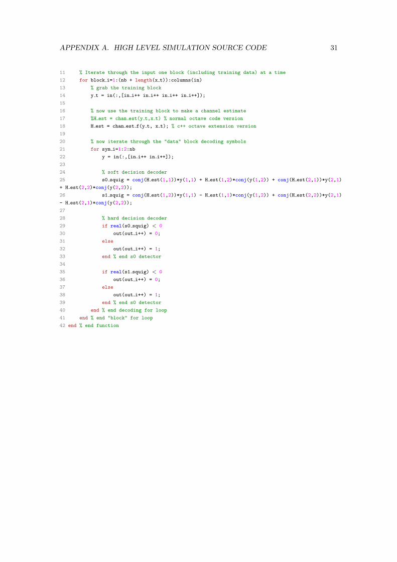
APPENDIX A. HIGH LEVEL SIMULATION SOURCE CODE 31
11 % Iterate through the input one block (including training data) at a time
12 for block i=1:(nb + length(x t)):columns(in)
13 % grab the training block
14 y t = in(:,[in i++ in i++ in i++ in i++]);
15
16 % now use the training block to make a channel estimate
17 %H est = chan est(y t,x t) % normal octave code version
18 H est = chan est f(y t, x t); % c++ octave extension version
19
20 % now iterate through the "data" block decoding symbols
21 for sym i=1:2:nb
22 y = in(:,[in i++ in i++]);
23
24 % soft decision decoder
25 s0 squig = conj(H est(1,1))*y(1,1) + H est(1,2)*conj(y(1,2)) + conj(H est(2,1))*y(2,1)
+ H est(2,2)*conj(y(2,2));
26 s1 squig = conj(H est(1,2))*y(1,1) - H est(1,1)*conj(y(1,2)) + conj(H est(2,2))*y(2,1)
- H est(2,1)*conj(y(2,2));
27
28 % hard decision decoder
29 if real(s0 squig) < 0
30 out(out i++) = 0;
31 else
32 out(out i++) = 1;
33 end % end s0 detector
34
35 if real(s1 squig) < 0
36 out(out i++) = 0;
37 else
38 out(out i++) = 1;
39 end % end s0 detector
40 end % end decoding for loop
41 end % end "block" for loop
42 end % end function

Appendix B
Low-Level Simulation Source
Code
Some of the source code used for the low-level simulation is presented in this appendix.For the sake of the trees producing the paper this report is printed on, not all of theheader files and associated supporting code is included.
B.1 BPSK Modulator
1 #include "bpsk const.h"
2
3 void bpsk mod(unsigned char input, unsigned char output re[8], unsigned char output im[8])
4 {5 unsigned short int i;
6
7 for(i=0; i<8; i++)
8 {9 /* test a single bit at a time */
10 if( (input>>i) & 0x01 )
11 {12 output re[i] = SYMBOL ONE RE;
13 output im[i] = SYMBOL ONE IM;
14 }15 else
16 {17 output re[i] = SYMBOL ZERO RE;
18 output im[i] = SYMBOL ZERO IM;
19 }20 }21 return;
22 }
32

APPENDIX B. LOW-LEVEL SIMULATION SOURCE CODE 33
B.2 Alamouti Encoder
1 #include <stdio.h>
2 #include "bpsk mod.h"
3
4 void alamouti enc(unsigned char input, char out re[2][8], char out im[2][8])
5 {6 int i=0;
7 unsigned char bpsk mod re[8], bpsk mod im[8];
8
9 /* modulate the block using BPSK */
10 bpsk mod(input, bpsk mod re, bpsk mod im);
11
12 for(i=0; i<8; i+=2)
13 {14 int i 1 = i + 1;
15
16 /* time t=T */
17 out re[0][i] = bpsk mod re[i];
18 out im[0][i] = bpsk mod im[i];
19
20 out re[1][i] = bpsk mod re[i 1];
21 out im[1][i] = bpsk mod im[i 1];
22
23 /* time t=T+1 */
24 out re[0][i 1] = -bpsk mod re[i 1];
25 out im[0][i 1] = bpsk mod im[i 1];
26
27 out re[1][i 1] = bpsk mod re[i];
28 out im[1][i 1] = -bpsk mod im[i];
29 }30 }
B.3 Channel Estimator
1 #include "chan est const.h"
2 #include "chan est.h"
3 #include "matrix.h"
4 #include "matrix fix.h"
5 #include "fixed.h"
6
7 void chan est(float rec re[TR ROWS][TR COLS], float rec im[TR ROWS][TR COLS], float *est re, float
*est im)
8 {9 /* I’m passing in the received training block, the transmitted training
10 * block, and the constant term are defined in "chan est.h"

APPENDIX B. LOW-LEVEL SIMULATION SOURCE CODE 34
11 */
12
13 comp matrix mult f((float *)rec re, (float *)rec im, TR ROWS, TR COLS, (float *)const term re,
(float *)const term im, CONST ROWS, CONST COLS, est re, est im);
14 }15
16 void chan est fix16(fix16 t rec re[TR ROWS][TR COLS], fix16 t rec im[TR ROWS][TR COLS], fix16 t *est re,
fix16 t *est im)
17 {18 fix16 t const term re 16[CONST ROWS][CONST COLS];
19 fix16 t const term im 16[CONST ROWS][CONST COLS];
20 int row,col;
21
22 /* make a fixed point version of the constant term */
23 for(row = 0; row < CONST ROWS; row++)
24 {25 for(col=0; col < CONST COLS; col++)
26 {27 const term re 16[row][col] = quantise 16bit l((const term re[row][col]));
28 const term im 16[row][col] = quantise 16bit l((const term im[row][col]));
29 }30 }31
32 comp matrix mult fix16((fix16 t *)rec re, (fix16 t *)rec im, TR ROWS, TR COLS, (fix16 t *)const term re 16,
(fix16 t *)const term im 16, CONST ROWS, CONST COLS, est re, est im);
33 }
B.4 Alamouti Decoder
1 #include "combiner.h"
2
3 #define COMB DEBUG 0
4
5 void combine( float recv re[2][2], float recv im[2][2],
6 float h re[2][2], float h im[2][2],
7 float symb re[2], float symb im[2] )
8 {9 symb re[0] = h re[0][0]*recv re[0][0] + h im[0][0]*recv im[0][0] +
10 h re[0][1]*recv re[0][1] + h im[0][1]*recv im[0][1] +
11 h re[1][0]*recv re[1][0] + h im[1][0]*recv im[1][0] +
12 h re[1][1]*recv re[1][1] + h im[1][1]*recv im[1][1] ;
13
14 symb im[0] = h re[0][0]*recv im[0][0] - h im[0][0]*recv re[0][0] -
15 h re[0][1]*recv im[0][1] + h im[0][1]*recv re[0][1] +
16 h re[1][0]*recv im[1][0] - h im[1][0]*recv re[1][0] -
17 h re[1][1]*recv im[1][1] + h im[1][1]*recv re[1][1] ;
18
19

APPENDIX B. LOW-LEVEL SIMULATION SOURCE CODE 35
20 symb re[1] = h re[0][1]*recv re[0][0] + h im[0][1]*recv im[0][0] -
21 h re[0][0]*recv re[0][1] - h im[0][0]*recv im[0][1] +
22 h re[1][1]*recv re[1][0] + h im[1][1]*recv im[1][0] -
23 h re[1][0]*recv re[1][1] - h im[1][0]*recv im[1][1] ;
24
25 symb im[1] = h re[0][1]*recv im[0][0] - h im[0][1]*recv re[0][0] +
26 h re[0][0]*recv im[0][1] - h im[0][0]*recv re[0][1] +
27 h re[1][1]*recv im[1][0] - h im[1][1]*recv re[1][0] +
28 h re[1][0]*recv im[1][1] - h im[1][0]*recv re[1][1] ;
29
30 return;
31 }32
33
34 void combine fix16(fix16 t recv re[2][2], fix16 t recv im[2][2],
35 fix16 t h re[2][2], fix16 t h im[2][2],
36 fix16 t symb re[2], fix16 t symb im[2] )
37 {38 long int temp re 0, temp re 1, temp im 0, temp im 1;
39
40
41 temp re 0 = fix16 mult(h re[0][0],recv re[0][0]) + fix16 mult(h im[0][0],recv im[0][0]) +
42 fix16 mult(h re[0][1],recv re[0][1]) + fix16 mult(h im[0][1],recv im[0][1]) +
43 fix16 mult(h re[1][0],recv re[1][0]) + fix16 mult(h im[1][0],recv im[1][0]) +
44 fix16 mult(h re[1][1],recv re[1][1]) + fix16 mult(h im[1][1],recv im[1][1]) ;
45
46 temp im 0 = fix16 mult(h re[0][0],recv im[0][0]) - fix16 mult(h im[0][0],recv re[0][0])-
47 fix16 mult(h re[0][1],recv im[0][1]) + fix16 mult(h im[0][1],recv re[0][1]) +
48 fix16 mult(h re[1][0],recv im[1][0]) - fix16 mult(h im[1][0],recv re[1][0]) -
49 fix16 mult(h re[1][1],recv im[1][1]) + fix16 mult(h im[1][1],recv re[1][1]) ;
50
51 temp re 1 = fix16 mult(h re[0][1],recv re[0][0]) + fix16 mult(h im[0][1],recv im[0][0]) -
52 fix16 mult(h re[0][0],recv re[0][1]) - fix16 mult(h im[0][0],recv im[0][1]) +
53 fix16 mult(h re[1][1],recv re[1][0]) + fix16 mult(h im[1][1],recv im[1][0]) -
54 fix16 mult(h re[1][0],recv re[1][1]) - fix16 mult(h im[1][0],recv im[1][1]) ;
55
56 temp im 1 = fix16 mult(h re[0][1],recv im[0][0]) - fix16 mult(h im[0][1],recv re[0][0]) +
57 fix16 mult(h re[0][0],recv im[0][1]) - fix16 mult(h im[0][0],recv re[0][1]) +
58 fix16 mult(h re[1][1],recv im[1][0]) - fix16 mult(h im[1][1],recv re[1][0]) +
59 fix16 mult(h re[1][0],recv im[1][1]) - fix16 mult(h im[1][0],recv re[1][1]) ;
60
61 symb re[0] = (fix16 t) temp re 0;
62 symb re[1] = (fix16 t) temp re 1;
63 symb im[0] = (fix16 t) temp im 0;
64 symb im[1] = (fix16 t) temp im 1;
65
66 return;
67 }

APPENDIX B. LOW-LEVEL SIMULATION SOURCE CODE 36
B.5 Fixed Point Functions
1 #include "fixed.h"
2
3 inline long int quantise 8bit l(float input)
4 {5 if (input >= (8))
6 return (long int) 127;
7 else if (input < (-8))
8 return (long int) -128;
9 else
10 return (long int) (input * (1 << RADIX 8));
11 }12
13 inline long int quantise 10bit l(float input)
14 {15 if (input >= (16))
16 return (long int) 255;
17 else if (input < (-16))
18 return (long int) -256;
19 return ((long int) (input * (1 << RADIX 10)));
20 }21
22 inline long int quantise 12bit l(float input)
23 {24 return ((long int) (input * (1 << RADIX 12)));
25 }26 inline long int quantise 16bit l(float input)
27 {28 return ((long int) (input * (1 << RADIX 16)));
29 }30
31 inline long int quantise 24bit l(float input)
32 {33 return ((long int) (input * (1 << RADIX 24)));
34 }35
36 inline float fix8 to float(fix8 t in)
37 {38 return ( in / (float) (1<<RADIX 8));
39 }40
41 inline float fix10 to float(fix10 t in)
42 {43 return ( in / (float) (1<<RADIX 10));
44 }45
46 inline float fix12 to float(fix12 t in)
47 {48 return ( in / (float) (1<<RADIX 12));
49 }

APPENDIX B. LOW-LEVEL SIMULATION SOURCE CODE 37
50 inline float fix16 to float(fix16 t in)
51 {52 return ( in / (float) (1<<RADIX 16));
53 }54
55 inline fix10 t fix8 to fix10(fix8 t in)
56 {57 return (fix10 t) ( in<<(RADIX 10 - RADIX 8) );
58 }59
60 inline fix12 t fix8 to fix12(fix8 t in)
61 {62 return (fix12 t) ( in<<(RADIX 12 - RADIX 8) );
63 }64
65 inline fix16 t fix8 to fix16(fix8 t in)
66 {67 return (fix16 t) ( in<<(RADIX 16 - RADIX 8) );
68 }69
70 inline fix12 t fix10 to fix12(fix10 t in)
71 {72 return (fix12 t) ( in<<(RADIX 12 - RADIX 10) );
73 }74
75 inline fix16 t fix10 to fix16(fix10 t in)
76 {77 return (fix16 t) ( in<<(RADIX 16 - RADIX 10) );
78 }79
80 inline fix16 t fix12 to fix16(fix12 t in)
81 {82 return (fix16 t) ( in<<(RADIX 16 - RADIX 12) );
83 }84
85 inline fix8 t fix8 mult(fix8 t a, fix8 t b)
86 {87 long int ans = 0;
88
89 ans = ((long int) a * (long int)b)>>RADIX 8;
90 #if FIXED DEBUG > 1
91 printf("fix8 mult: Real - %f * %f = %f (%f => 0x%lx)\n",fix8 to float(a),
92 fix8 to float(b), fix8 to float(ans) , fix8 to float(a) * fix8 to float(b),
93 quantise 8bit l(fix8 to float(a) * fix8 to float(b)));
94
95 printf("fix8 mult: Int - %d * %d = %ld\n",a,b,ans);96 printf("fix8 mult: Hex - 0x%x * 0x%x = 0x%lx\n",a,b,ans);97 #endif
98
99 #if FIXED DEBUG > 0
100 if (ans > 0x7f)
APPENDIX B. LOW-LEVEL SIMULATION SOURCE CODE 38
101 {102 printf("Overflow trying to do fix8 mult: 0x%x * 0x%x ?= 0x%lx\n",a,b,ans);103 exit(-1);
104 }105 #endif
106 return (fix8 t) ans;
107 }108
109
110 inline fix16 t fix16 mult(fix16 t a, fix16 t b)
111 {112 long int ans = 0;
113
114 ans = ((long int) a * (long int)b)>>RADIX 16;
115 #if FIXED DEBUG > 0
116 printf("[0x%x * 0x%x = 0x%x]",(unsigned short)a,(unsigned short)b,(unsigned short)ans);
117 #endif
118 return (fix16 t) ans;
119 }120
121 inline fix10 t fix10 mult(fix10 t a, fix10 t b)
122 {123 long int ans = 0;
124
125 ans = ((long int) a * (long int)b)>>RADIX 10;
126 return (fix10 t) ans;
127 }128
129 inline fix12 t fix12 mult(fix12 t a, fix12 t b)
130 {131 long int ans = 0;
132
133 ans = ((long int) a * (long int)b)>>RADIX 12;
134 return (fix12 t) ans;
135 }

Appendix C
Hardware Design Source Code
This Appendix contains the current1 source code used for the hardware designs. Thecode is written in VHDL and has bee tested and synthesised using the no cost “Web-Pack” tools available from Xilinx.
C.1 BPSK Modulator
1 library ieee;
2 use ieee.std logic 1164.all;
3 use ieee.std logic arith.all;
4
5 entity bpsk mod is port (
6 input : in std logic;
7 i out, q out : out signed(7 downto 0)
8 );
9 end bpsk mod;
10
11 architecture a of bpsk mod is
12 begin
13 with input select i out <=
14 "01111111" when ’1’,
15 "10000000" when others;
16 q out <= "00000000";
17 end a;
18
1current at time of report writing
39

APPENDIX C. HARDWARE DESIGN SOURCE CODE 40
C.2 BPSK Demodulator
1 library ieee;
2 use ieee.std logic 1164.all;
3 use ieee.std logic arith.all;
4
5 entity bpsk demod is port (
6 i in,q in : in signed(7 downto 0);
7 output : out std logic
8 );
9 end bpsk demod;
10
11 architecture a of bpsk demod is
12 begin
13 output <= not i in(7);
14 end a;
15
C.3 Alamouti Enoder
1 library ieee;
2 use ieee.std logic 1164.all;
3 use ieee.std logic arith.all;
4
5
6 entity alamouti mod is
7 port
8 (
9 clk : in std logic;
10 i1 in,i2 in : in signed(7 downto 0);
11 q1 in,q2 in : in signed(7 downto 0);
12 i1 out,q1 out : in signed(7 downto 0);
13 i2 out,q2 out : in signed(7 downto 0)
14 );
15 end alamouti mod;
16
17 architecture a of alamouti mod is
18 signal tmp1 i, tmp1 q : signed(7 downto 0); -- antenna1 variables
19 signal tmp2 i, tmp2 q : signed(7 downto 0); -- antenna2 variables
20 signal state : std logic;
21 begin
22 process(clk)
23 begin
24 if (clk’event and clk = ’1’) then
25 if (state = ’0’) then-- first cycle
26 tmp1 i <= i1 in;
27 tmp1 q <= q1 in;
28
29 tmp2 i <= i2 in;

APPENDIX C. HARDWARE DESIGN SOURCE CODE 41
30 tmp2 q <= q2 in;
31 state <= ’1’;
32 else
33 tmp1 i <= -i2 in;
34 tmp1 q <= q2 in;
35
36 tmp2 i <= i1 in;
37 tmp2 q <= -q1 in;
38 state <= ’0’;
39 end if;
40 end if;
41 end process;
42
43
44 i1 out <= tmp1 i;
45 q1 out <= tmp1 q;
46
47 i2 out <= tmp2 i;
48 q2 out <= tmp2 q;
49 end a;
50
C.4 Alamouti Decoder
1 library IEEE;
2 use IEEE.STD LOGIC 1164.ALL;
3 use IEEE.STD LOGIC ARITH.ALL;
4 use IEEE.STD LOGIC SIGNED.ALL;
5
6
7 library work;
8 use work.my types.all;
9
10 entity combiner is port (
11 clock : in std logic;
12 reset : in std logic;
13
14 rx re in : in t 2x2 matrix 16;
15 rx im in : in t 2x2 matrix 16;
16 h re in : in t 2x2 matrix 16;
17 h im in : in t 2x2 matrix 16;
18
19 s0re est : out std logic vector(15 downto 0);
20 s0im est : out std logic vector(15 downto 0);
21 s1re est : out std logic vector(15 downto 0);
22 s1im est : out std logic vector(15 downto 0);
23
24 -- debug : out std logic vector(15 downto 0);

APPENDIX C. HARDWARE DESIGN SOURCE CODE 42
25
26 done : out std logic
27 );
28 end combiner;
29
30 architecture Behavioral of combiner is
31 signal s0re op : std logic;
32 signal s0im op : std logic;
33 signal s1re op : std logic;
34 signal s1im op : std logic;
35
36 signal clear control : std logic;
37 signal clear units : std logic;
38 signal add clear : std logic;
39
40 signal op a : std logic vector(15 downto 0);
41 signal op b : std logic vector(15 downto 0);
42 signal op c : std logic vector(15 downto 0);
43 signal op d : std logic vector(15 downto 0);
44
45 signal s0re prod : std logic vector(15 downto 0);
46 signal s0im prod : std logic vector(15 downto 0);
47 signal s1re prod : std logic vector(15 downto 0);
48 signal s1im prod : std logic vector(15 downto 0);
49
50 signal s0re sum : std logic vector(15 downto 0);
51 signal s0im sum : std logic vector(15 downto 0);
52 signal s1re sum : std logic vector(15 downto 0);
53 signal s1im sum : std logic vector(15 downto 0);
54
55 signal s0re total : std logic vector(15 downto 0);
56 signal s0im total : std logic vector(15 downto 0);
57 signal s1re total : std logic vector(15 downto 0);
58 signal s1im total : std logic vector(15 downto 0);
59
60 signal s0re op regd : std logic;
61 signal s0im op regd : std logic;
62 signal s1re op regd : std logic;
63 signal s1im op regd : std logic;
64
65 signal add count : integer range 0 to 7;
66 signal done i : std logic;
67 -------------------------------------------------
68 -- component declarations --
69 -------------------------------------------------
70 component comb control
71 port(
72 clock : in std logic;
73 reset : in std logic;
74
75 rx re in : in t 2x2 matrix 16;

APPENDIX C. HARDWARE DESIGN SOURCE CODE 43
76 rx im in : in t 2x2 matrix 16;
77 h re in : in t 2x2 matrix 16;
78 h im in : in t 2x2 matrix 16;
79
80 operand a : out std logic vector(15 downto 0);
81 operand b : out std logic vector(15 downto 0);
82 operand c : out std logic vector(15 downto 0);
83 operand d : out std logic vector(15 downto 0);
84
85 s0re add, s0im add: out std logic;
86 s1re add, s1im add: out std logic;
87 done : out std logic;
88 clear : out std logic
89 );
90 end component;
91
92 component add sub 16 is port (
93 a : in std logic vector(15 downto 0);
94 b : in std logic vector(15 downto 0);
95 add : in std logic;
96 ans : out std logic vector(15 downto 0)
97 );end component;
98 ---------------- end component declarations ------------------
99 begin
100
101 clear units <= reset or clear control;
102
103 combiner control unit: comb control port map(
104 clock => clock,
105 reset => reset,
106 rx re in => rx re in,
107 rx im in => rx im in,
108 h re in => h re in,
109 h im in => h im in,
110
111 operand a => op a,
112 operand b => op b,
113 operand c => op c,
114 operand d => op d,
115
116 s0re add => s0re op,
117 s0im add => s0im op,
118 s1re add => s1re op,
119 s1im add => s1im op,
120 done => done i,
121 clear => clear control
122 );
123 done <= done i;
124
125 -- need to register the add/subtract signals because
126 -- the product gets registered, need to keep them in

APPENDIX C. HARDWARE DESIGN SOURCE CODE 44
127 -- sync!
128 process (clock)
129 begin
130 if (clock’event and clock=’1’) then
131 s0re op regd <= s0re op;
132 s0im op regd <= s0im op;
133 s1re op regd <= s1re op;
134 s1im op regd <= s1im op;
135 end if;
136 end process;
137
138 -------------------------------------------
139 -- Multipliers and registers
140 -------------------------------------------
141 s0re mult: process (clock)
142 variable result : signed(31 downto 0);
143 begin
144 if(clock’event and clock = ’1’) then
145 result := conv signed(conv integer(op a) * conv integer(op b), 32);
146 s0re prod <= conv std logic vector(result(23 downto 8),16);
147 end if;
148 end process;
149
150 s0im mult: process (clock)
151 variable result : signed(31 downto 0);
152 begin
153 if(clock’event and clock = ’1’) then
154 result := conv signed( conv integer(op a) * conv integer(op c) ,32);
155 s0im prod <= conv std logic vector(result(23 downto 8),16);
156 end if;
157 end process;
158
159 s1re mult: process (clock)
160 variable result : signed(31 downto 0);
161 begin
162 if(clock’event and clock = ’1’) then
163 result := conv signed( conv integer(op d) * conv integer(op b), 32);
164 s1re prod <= conv std logic vector(result(23 downto 8),16);
165 end if;
166 end process;
167
168 s1im mult: process (clock)
169 variable result : signed(31 downto 0);
170 begin
171 if(clock’event and clock = ’1’) then
172 result := conv signed( conv integer(op d) * conv integer(op c), 32);
173 s1im prod <= conv std logic vector(result(23 downto 8),16);
174 end if;
175 end process;
176
177 -----------------------------------------

APPENDIX C. HARDWARE DESIGN SOURCE CODE 45
178 -- Adders / Subtracters
179 -----------------------------------------
180 s0re add: add sub 16 port map (
181 a => s0re total,
182 b => s0re prod,
183 add => s0re op regd,
184 ans => s0re sum
185 );
186
187 s0im add: add sub 16 port map (
188 a => s0im total,
189 b => s0im prod,
190 add => s0im op regd,
191 ans => s0im sum
192 );
193 s1re add: add sub 16 port map (
194 a => s1re total,
195 b => s1re prod,
196 add => s1re op regd,
197 ans => s1re sum
198 );
199
200 s1im add: add sub 16 port map (
201 a => s1im total,
202 b => s1im prod,
203 add => s1im op regd,
204 ans => s1im sum
205 );
206 -----------------------------------------
207 -- Registers
208 -----------------------------------------
209 s0re reg: process (clock)
210 begin
211 if(clock’event and clock = ’1’ ) then
212 if (clear units =’1’) then
213 s0re total <= x"0000";
214 else
215 s0re total <= s0re sum;
216 end if;
217 end if;
218 end process;
219
220 s0im reg: process (clock)
221 begin
222 if(clock’event and clock = ’1’ ) then
223 if (clear units =’1’) then
224 s0im total <= x"0000";
225 else
226 s0im total <= s0im sum;
227 end if;
228 end if;

APPENDIX C. HARDWARE DESIGN SOURCE CODE 46
229 end process;
230
231 s1re reg: process (clock)
232 begin
233 if(clock’event and clock = ’1’ ) then
234 if (clear units =’1’) then
235 s1re total <= x"0000";
236 else
237 s1re total <= s1re sum;
238 end if;
239 end if;
240 end process;
241
242 s1im reg: process (clock)
243 begin
244 if(clock’event and clock = ’1’ ) then
245 if (clear units =’1’) then
246 s1im total <= x"0000";
247 else
248 s1im total <= s1im sum;
249 end if;
250 end if;
251 end process;
252
253
254 ----------------------------------------------
255 -- output assignements
256 ----------------------------------------------
257
258 s0re est <= s0re sum;
259 s0im est <= s0im sum;
260 s1re est <= s1re sum;
261 s1im est <= s1im sum;
262
263 --debug <= x"000" & s0re op regd & s0im op regd & s1re op regd & s1im op regd;
264 --debug <= x"000" & ’0’ &’0’ &’0’ & clear control;
265 end Behavioral;
C.4.1 Control Unit
1 library IEEE;
2 use IEEE.STD LOGIC 1164.ALL;
3 use IEEE.STD LOGIC ARITH.ALL;
4 use IEEE.STD LOGIC UNSIGNED.ALL;
5
6 library work;
7 use work.my types.all;
8
9 entity comb control is Port (

APPENDIX C. HARDWARE DESIGN SOURCE CODE 47
10 clock : in std logic;
11 reset : in std logic;
12
13 rx re in : in t 2x2 matrix 16;
14 rx im in : in t 2x2 matrix 16;
15 h re in : in t 2x2 matrix 16;
16 h im in : in t 2x2 matrix 16;
17
18
19 -- Key:
20 -- A -> s0 re op1, s0 im op1
21 -- B -> s0 re op2, s1 re op2
22 -- C -> s0 im op2, s1 im op2
23 -- D -> s1 re op1, s1 im op1
24 operand a : out std logic vector(15 downto 0);
25 operand b : out std logic vector(15 downto 0);
26 operand c : out std logic vector(15 downto 0);
27 operand d : out std logic vector(15 downto 0);
28
29 s0re add, s0im add: out std logic;
30 s1re add, s1im add: out std logic;
31 done : out std logic;
32 clear : out std logic
33 );
34 end comb control;
35
36 architecture Behavioral of comb control is
37 type state type is (st rst,st1, st2, st3, st4, st5, st6, st7, st8);
38 -- state machine internal signals
39 signal state, next state : state type;
40 signal op a i : std logic vector(15 downto 0);
41 signal op b i : std logic vector(15 downto 0);
42 signal op c i : std logic vector(15 downto 0);
43 signal op d i : std logic vector(15 downto 0);
44
45 signal s0re add i, s0im add i : std logic;
46 signal s1re add i, s1im add i : std logic;
47
48 signal rx re reg, rx im reg : t 2x2 matrix 16;
49 signal h re reg, h im reg : t 2x2 matrix 16;
50
51
52 -- temp output logic signals
53 signal done i : std logic;
54 signal clear i : std logic;
55 begin
56 input regs : process (clock,reset)
57 begin
58 if(clock’event and clock=’1’) then
59 if (reset = ’1’) then
60 rx re reg <= (others => x"0000");

APPENDIX C. HARDWARE DESIGN SOURCE CODE 48
61 rx im reg <= (others => x"0000");
62 h re reg <= (others => x"0000");
63 h im reg <= (others => x"0000");
64 elsif (state = st8) or (state = st rst) then
65 rx re reg <= rx re in;
66 rx im reg <= rx im in;
67 h re reg <= h re in;
68 h im reg <= h im in;
69 end if;
70 end if;
71 end process;
72
73
74 SYNC PROC: process (CLOCK, reset)
75 begin
76 if (clock’event and clock = ’1’) then
77 if ( reset = ’1’ ) then
78 state <= st rst;
79 s0re add <= ’1’;
80 s0im add <= ’1’;
81 s1re add <= ’1’;
82 s1im add <= ’1’;
83
84 operand a <= x"0000";
85 operand b <= x"0000";
86 operand c <= x"0000";
87 operand d <= x"0000";
88
89 done <= ’0’;
90 clear <= ’1’;
91 else
92 state <= next state;
93
94 s0re add <= s0re add i;
95 s0im add <= s0im add i;
96 s1re add <= s1re add i;
97 s1im add <= s1im add i;
98
99 done <= done i;
100 clear <= clear i;
101
102 operand a <= op a i;
103 operand b <= op b i;
104 operand c <= op c i;
105 operand d <= op d i;
106 end if;
107 end if;
108 end process;
109
110
111 --MOORE State Machine - Outputs based on state only
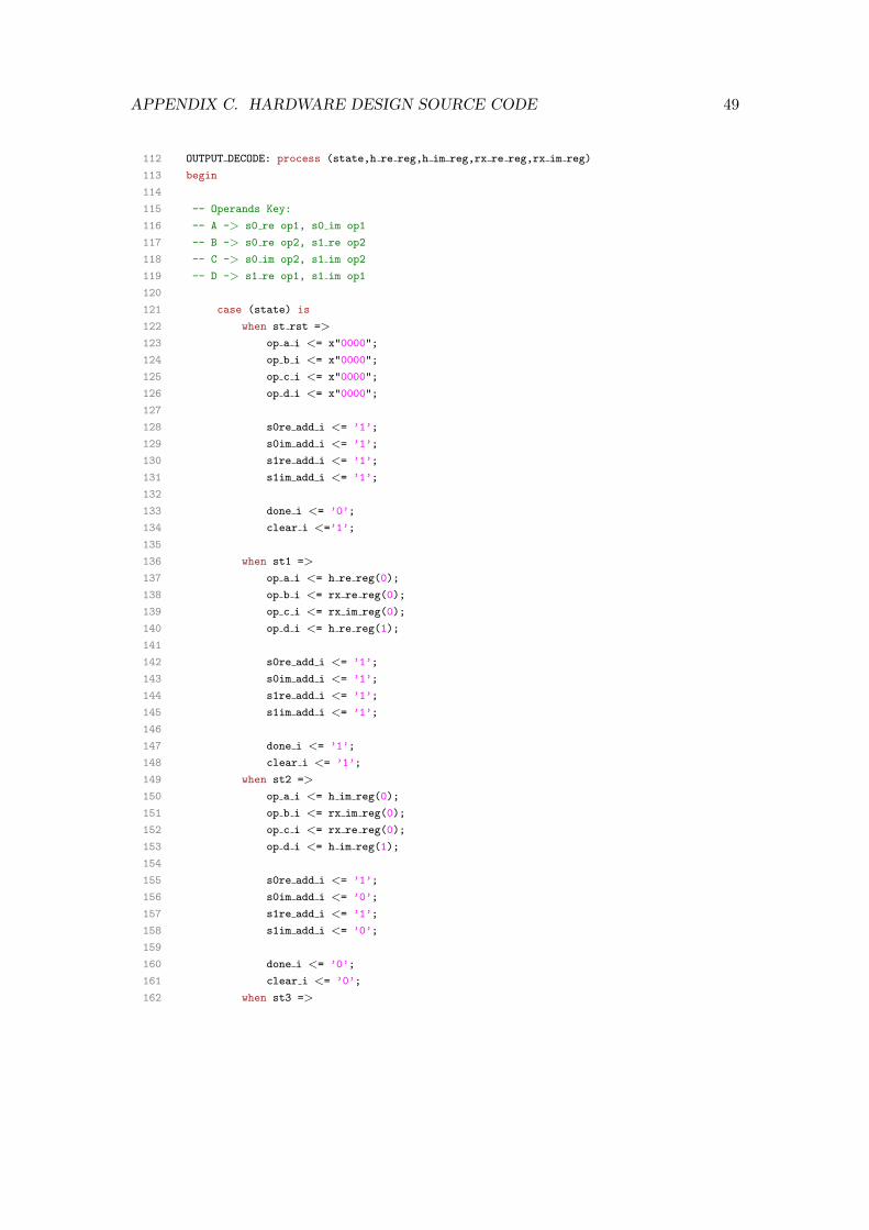
APPENDIX C. HARDWARE DESIGN SOURCE CODE 49
112 OUTPUT DECODE: process (state,h re reg,h im reg,rx re reg,rx im reg)
113 begin
114
115 -- Operands Key:
116 -- A -> s0 re op1, s0 im op1
117 -- B -> s0 re op2, s1 re op2
118 -- C -> s0 im op2, s1 im op2
119 -- D -> s1 re op1, s1 im op1
120
121 case (state) is
122 when st rst =>
123 op a i <= x"0000";
124 op b i <= x"0000";
125 op c i <= x"0000";
126 op d i <= x"0000";
127
128 s0re add i <= ’1’;
129 s0im add i <= ’1’;
130 s1re add i <= ’1’;
131 s1im add i <= ’1’;
132
133 done i <= ’0’;
134 clear i <=’1’;
135
136 when st1 =>
137 op a i <= h re reg(0);
138 op b i <= rx re reg(0);
139 op c i <= rx im reg(0);
140 op d i <= h re reg(1);
141
142 s0re add i <= ’1’;
143 s0im add i <= ’1’;
144 s1re add i <= ’1’;
145 s1im add i <= ’1’;
146
147 done i <= ’1’;
148 clear i <= ’1’;
149 when st2 =>
150 op a i <= h im reg(0);
151 op b i <= rx im reg(0);
152 op c i <= rx re reg(0);
153 op d i <= h im reg(1);
154
155 s0re add i <= ’1’;
156 s0im add i <= ’0’;
157 s1re add i <= ’1’;
158 s1im add i <= ’0’;
159
160 done i <= ’0’;
161 clear i <= ’0’;
162 when st3 =>

APPENDIX C. HARDWARE DESIGN SOURCE CODE 50
163 op a i <= h re reg(1);
164 op b i <= rx re reg(1);
165 op c i <= rx im reg(1);
166 op d i <= h re reg(0);
167
168 s0re add i <= ’1’;
169 s0im add i <= ’0’;
170 s1re add i <= ’0’;
171 s1im add i <= ’1’;
172
173 done i <= ’0’;
174 clear i <= ’0’;
175 when st4 =>
176 op a i <= h im reg(1);
177 op b i <= rx im reg(1);
178 op c i <= rx re reg(1);
179 op d i <= h im reg(0);
180
181 s0re add i <= ’1’;
182 s0im add i <= ’1’;
183 s1re add i <= ’0’;
184 s1im add i <= ’0’;
185
186 done i <= ’0’;
187 clear i <= ’0’;
188 when st5 =>
189 op a i <= h re reg(2);
190 op b i <= rx re reg(2);
191 op c i <= rx im reg(2);
192 op d i <= h re reg(3);
193
194 s0re add i <= ’1’;
195 s0im add i <= ’1’;
196 s1re add i <= ’1’;
197 s1im add i <= ’1’;
198
199 done i <= ’0’;
200 clear i <= ’0’;
201 when st6 =>
202 op a i <= h im reg(2);
203 op b i <= rx im reg(2);
204 op c i <= rx re reg(2);
205 op d i <= h im reg(3);
206
207 s0re add i <= ’1’;
208 s0im add i <= ’0’;
209 s1re add i <= ’1’;
210 s1im add i <= ’0’;
211
212 done i <= ’0’;
213 clear i <= ’0’;

APPENDIX C. HARDWARE DESIGN SOURCE CODE 51
214 when st7 =>
215 op a i <= h re reg(3);
216 op b i <= rx re reg(3);
217 op c i <= rx im reg(3);
218 op d i <= h re reg(2);
219
220 s0re add i <= ’1’;
221 s0im add i <= ’0’;
222 s1re add i <= ’0’;
223 s1im add i <= ’1’;
224
225 done i <= ’0’;
226 clear i <= ’0’;
227 when st8 =>
228 op a i <= h im reg(3);
229 op b i <= rx im reg(3);
230 op c i <= rx re reg(3);
231 op d i <= h im reg(2);
232
233 s0re add i <= ’1’;
234 s0im add i <= ’1’;
235 s1re add i <= ’0’;
236 s1im add i <= ’0’;
237 clear i <= ’0’;
238 done i <= ’0’;
239 end case;
240 end process;
241
242 NEXT STATE DECODE: process (state)
243 begin
244 --declare default state for next state to avoid latches
245 next state <= state; --default is to stay in current state
246 case (state) is
247 when st rst => next state <= st1;
248 when st1 => next state <= st2;
249 when st2 => next state <= st3;
250 when st3 => next state <= st4;
251 when st4 => next state <= st5;
252 when st5 => next state <= st6;
253 when st6 => next state <= st7;
254 when st7 => next state <= st8;
255 when st8 => next state <= st1;
256 when others =>
257 next state <= st rst;
258 end case;
259 end process;
260
261 end Behavioral;
APPENDIX C. HARDWARE DESIGN SOURCE CODE 52
C.4.2 Add/Subtract Unit
1 library IEEE;
2 use IEEE.STD LOGIC 1164.ALL;
3 use IEEE.STD LOGIC ARITH.ALL;
4 use IEEE.STD LOGIC SIGNED.ALL;
5
6
7 entity add sub 16 is
8 Port ( a : in std logic vector(15 downto 0);
9 b : in std logic vector(15 downto 0);
10 add : in std logic;
11 ans : out std logic vector(15 downto 0)
12 );
13 end add sub 16;
14
15 architecture Behavioral of add sub 16 is
16 begin
17 process(a,b,add)
18 variable op b : std logic vector(15 downto 0);
19 variable carry in : std logic;
20 begin
21 -- This way uses 33 of 3072 slices, and has a delay of 13.425ns
22 -- if(add = ’1’) then
23 -- ans <= a + b;
24 -- else
25 -- ans <= a - b;
26 -- end if;
27
28 -- This way uses 17/3072 slices, and 31/6144 4in-LUTs, delay of 13ns
29 if (add = ’1’) then
30 op b := b;
31 carry in := ’0’;
32 else
33 op b := not b;
34 carry in := ’1’;
35 end if;
36 ans <= a + op b + carry in;
37 end process;
38 end Behavioral;

Bibliography
[1] David Gesbert, Mansoor Shafi, Da-shan Shiu, Peter J. Smith, and Ayman Naguib.From theory to practice: An overview of mimo space-time coded wireless systems.IEEE Journal on Selected Areas in Communications, 21(3):281–302, 2003.
[2] Erik G. Larsen and Petre Stoica. Space-Time Block Coding for Wireless Communi-cations. Cambridge University Press, 2003.
[3] Hesham El Gamal and A. Roger Hammons, Jr. On the Design and Performance ofAlgebraic Space-Time Codes for BPSK and QPSK Modulation. IEEE Transactionson Communications, 50(8):907–913, June 2002.
[4] Markus Rupp, Andreas Burg, Eric Beck. Rapid Prototyping for Wireless Designs:the Five-Ones Approach. Signal Processing, 83:1427–1444, 2003.
[5] Raghu Mysore Rao et. al. Multi-Antenna Testbeds for Research and Education inWireless Communications. IEEE Communications Magazine, pages 72–81, December2004.
[6] Raleigh, G.G. and Cioffi, J.M. . Spatio-temporal coding for wireless communications.IEEE Transactions on Communications, 46(3):357–366, 1998.
[7] Siavash M. Alamouti. A Simple Transmit Diversity Technique for Wireless Com-munications. IEEE Journal on Select Areas in Communcations, 16(8):1451–1458,October 1998.
[8] Vahid Tarokh, Hamid Jafarkhani, and A. Robert Calderbank. Space-time blockcoding for wireless communications: Performance results. IEEE Journal on SelectedAreas in Communications, 17(3):451–460, March 1999.
53