Fourier Optics in Examples - uni-osnabrueck.de · Fourier Optics in Examples FOURIER. ... (for a...

UNIVERSITAT� OSNABRUCK 1

Fourier Optics in Examples FOURIER.TEX KB 20020205

KLAUS BETZLER1 , FACHBEREICH PHYSIK, UNIVERSITAT OSNABRUCK

This short lecture note presents some two-dimensional optical structures and theircalculated Fourier transforms. These can be regarded as the respective far-fielddiffraction patterns. As an addition to textbooks, it may present some visual helpto students working in the field of optics.

1 Paraxial Approximation

When light is propagating (here in positive �-direction), the electric field in anarbitrary plane at � can be calculated from the field at any preceding plane at ��applying Huygens’s construction.

Figure 1: Geometry and parameters used in Eq. 1 for the paraxial approximation.Light is propagating from left to right (� � ��).

The geometry is sketched in Fig: 1, for the field at � � �� contributed by thepoint �� one may derive

��

�� (1)

assuming monochromatic, coherent light. Furthermore, we assume scalar �, whichmeans that we consider only one polarization component and light propagationapproximately parallel to the �-axis.

To get the total field, we have to integrate over �� and �� in the ��-plane

��

��

��

��

��

��

�� (2)

Here��

�� (3)

[email protected]

2 FACHBEREICH PHYSIK

can be approximated if we assume that

��

� � �� (4)

– this is called Paraxial Approximation – to

��

��

��

�� (5)

� ��

��

��

�

��

� (6)

Thus, using

��

��

��

�

��

�(7)

and

��

��

��

�

��

�

� ��

��

��

��

��

��

��

� � ��

��

��

��

�

��

�� (8)

Eq. 2 can be written as

��

� � ��

� ��

��

��

� � ��

�� (9)

where

� ��

��

��

��

� (10)

Eq. 9 can be interpreted as a sequence of three operations:

� The field �� is multiplied by a phase factor � �� .

� For this product a two-dimensional Fourier transform is calculated.

� The result is multiplied by a second phase factor � �� .

If the approximations leading to Eq. 9 can be made, this is called Fresnel Diffrac-tion or Fresnel Approximation (for a more detailed introduction together with somesample calculations see e. g. [1]).

If, in addition, we can assume that � �� in the entire region considered,i e. that � � �� is large enough, Eq. 9 can be rewritten as

��

� � ��

� ��

��

��

� � ��

�� (11)


In this regime, �� is just the two-dimensional Fourier transform of ��

except for a multiplicative phase factor which does not affect the intensity of thelight. This regime is called Fraunhofer Diffraction or Fraunhofer Approximation.The examples presented here are calculated numerically assuming Fraunhofer ap-proximation, i. e. simple two-dimensional Fourier transform.

2 Basic Features

First some basic features of the Fourier transform in two dimensions are outlined.

2.1 Dimensionality

When the two-dimensional pattern is only structured in one dimension, that alsoshows up in the Fourier transform, yet in a reciprocal meaning. This is visualizedby Figs. 2 and 3.

Figure 2: Array of lines (left) and the corresponding two-dimensional Fouriertransform (right).

Figure 3: Array of points (left) and the corresponding two-dimensional Fouriertransform (right).

In Fig. 2 the pattern is constant in the vertical dimension, its Fourier transformshows a delta function behavior in this dimension, yielding a linear array of points.Vice versa for Fig. 3. That’s due to the fact that the Fourier transform of a constantis the delta function and vice versa.

2.2 Number of Elements

The number of elements in the original pattern strongly determines the sharpnessof the diffraction pattern. Fig. 4 demonstrates this using a one-dimensional regularstructure of points as source pattern. Depending on the number of points used, thediffraction pattern varies in sharpness.


Figure 4: Dependence of the diffraction pattern on the number of source objectsused. The sharpness increases with this number (from top to bottom: 3, 5, 7, 9, 11,13, 15, 17, 19).

2.3 Apodization

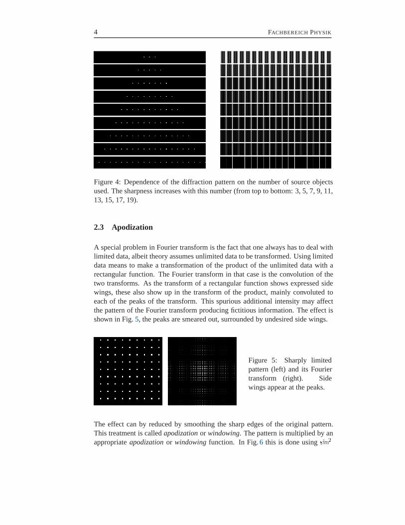
A special problem in Fourier transform is the fact that one always has to deal withlimited data, albeit theory assumes unlimited data to be transformed. Using limiteddata means to make a transformation of the product of the unlimited data with arectangular function. The Fourier transform in that case is the convolution of thetwo transforms. As the transform of a rectangular function shows expressed sidewings, these also show up in the transform of the product, mainly convoluted toeach of the peaks of the transform. This spurious additional intensity may affectthe pattern of the Fourier transform producing fictitious information. The effect isshown in Fig. 5, the peaks are smeared out, surrounded by undesired side wings.

Figure 5: Sharply limitedpattern (left) and its Fouriertransform (right). Sidewings appear at the peaks.

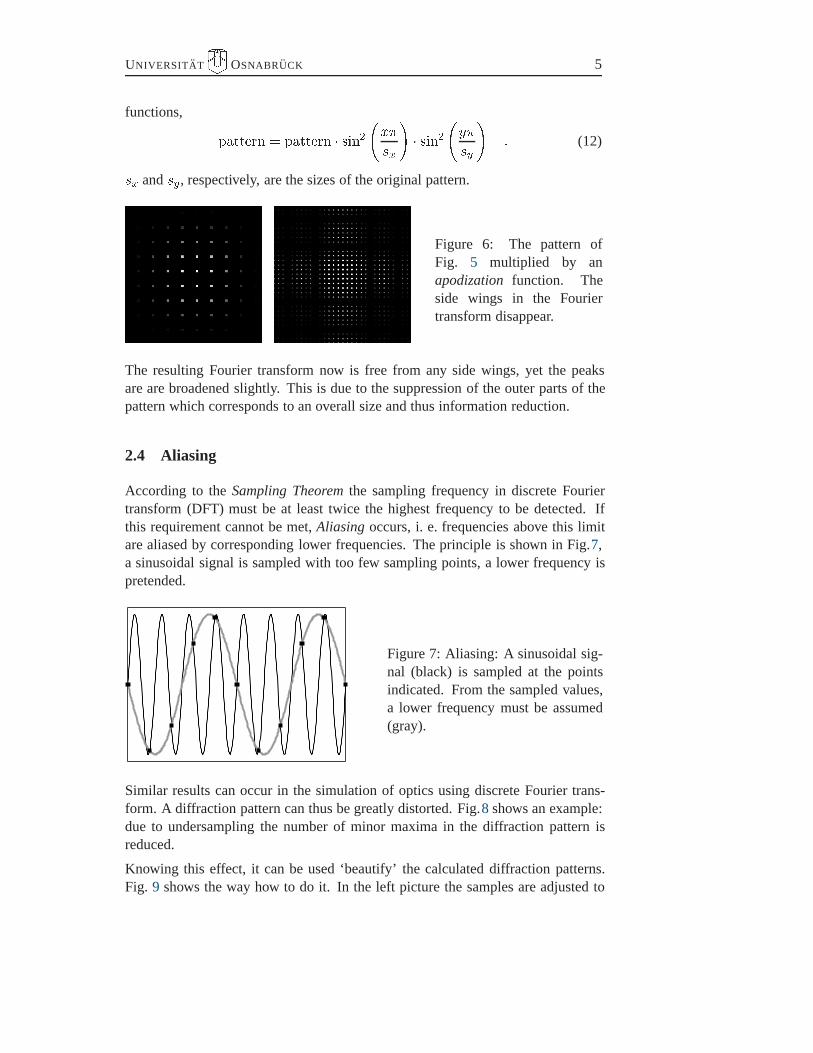
The effect can by reduced by smoothing the sharp edges of the original pattern.This treatment is called apodization or windowing. The pattern is multiplied by anappropriate apodization or windowing function. In Fig. 6 this is done using ��


functions,

��

�

��

��

�

� (12)

� and �, respectively, are the sizes of the original pattern.

Figure 6: The pattern ofFig. 5 multiplied by anapodization function. Theside wings in the Fouriertransform disappear.

The resulting Fourier transform now is free from any side wings, yet the peaksare are broadened slightly. This is due to the suppression of the outer parts of thepattern which corresponds to an overall size and thus information reduction.

2.4 Aliasing

According to the Sampling Theorem the sampling frequency in discrete Fouriertransform (DFT) must be at least twice the highest frequency to be detected. Ifthis requirement cannot be met, Aliasing occurs, i. e. frequencies above this limitare aliased by corresponding lower frequencies. The principle is shown in Fig.7,a sinusoidal signal is sampled with too few sampling points, a lower frequency ispretended.

Figure 7: Aliasing: A sinusoidal sig-nal (black) is sampled at the pointsindicated. From the sampled values,a lower frequency must be assumed(gray).

Similar results can occur in the simulation of optics using discrete Fourier trans-form. A diffraction pattern can thus be greatly distorted. Fig.8 shows an example:due to undersampling the number of minor maxima in the diffraction pattern isreduced.

Knowing this effect, it can be used ‘beautify’ the calculated diffraction patterns.Fig. 9 shows the way how to do it. In the left picture the samples are adjusted to


Figure 8: Undersampling of adiffraction pattern: Only 3 minormaxima instead of 13 seem to bepresent.

get a background-free diffraction pattern, in the right picture the number of samplesis doubled to get an exact representation of the pattern.

Figure 9: ‘Background-free’ Fourier transform of a grating structure using an ap-propriately adjusted sample density (left) compared to a reasonable representationof the structure using doubled sample density (right).

It can be calculated that we get the background-free representation when the to-tal size of the pattern to be transformed equates exactly a multiple of the period.Fig: 10 shows this situation, the total size is 360, the period of the structure is12 points. The Fourier transform of the grating structure is sharp and free of anyminor maxima.

Figure 10: Grating structure with a multiple-period size. The Fourier transform issharp and background-free.

If we don’t meet this condition exactly, spurious intensity between the main peaksis produced. In Fig. 11 a period size of 13 with a total size of 360 points is used tovisualize this.

The total number of samples in the Fourier transform equates the number of pointsin the original. The way to get a higher density of samples without adding morediffracting elements (which would also refine the diffraction pattern) is called Zero


Figure 11: Grating structure with a size not equal to a multiple of the period (left),and corresponding Fourier tranform (right).

Padding. In the original an appropriate number of zeros is added to get the desirednumber of samples. To double the sample number, e. g., a zero matrix with thesame size as the original has to be joined (Fig.12).

Figure 12: Zero padding: Grating structure of Fig. 10 padded with a zero matrix ofthe same size. In the Fourier transform the minor structures of the pattern are nowvisible.

2.5 Element Size

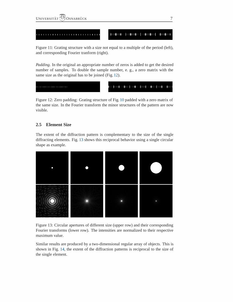
The extent of the diffraction pattern is complementary to the size of the singlediffracting elements. Fig. 13 shows this reciprocal behavior using a single circularshape as example.

Figure 13: Circular apertures of different size (upper row) and their correspondingFourier transforms (lower row). The intensities are normalized to their respectivemaximum value.

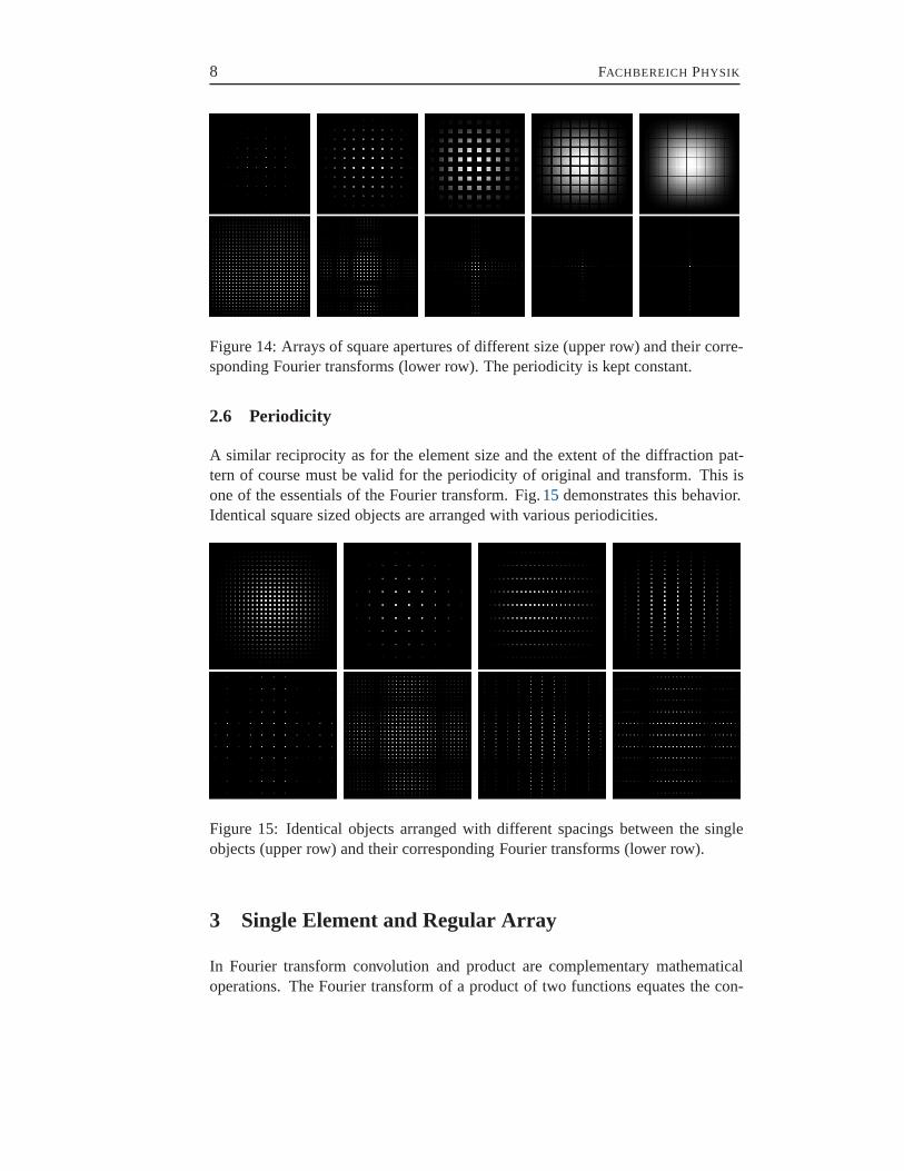
Similar results are produced by a two-dimensional regular array of objects. This isshown in Fig. 14, the extent of the diffraction patterns is reciprocal to the size ofthe single element.


Figure 14: Arrays of square apertures of different size (upper row) and their corre-sponding Fourier transforms (lower row). The periodicity is kept constant.

2.6 Periodicity

A similar reciprocity as for the element size and the extent of the diffraction pat-tern of course must be valid for the periodicity of original and transform. This isone of the essentials of the Fourier transform. Fig. 15 demonstrates this behavior.Identical square sized objects are arranged with various periodicities.

Figure 15: Identical objects arranged with different spacings between the singleobjects (upper row) and their corresponding Fourier transforms (lower row).

3 Single Element and Regular Array

In Fourier transform convolution and product are complementary mathematicaloperations. The Fourier transform of a product of two functions equates the con-


volution of the Fourier transforms of the two functions. Vice versa, the Fouriertransform of a convolution of two functions equates the product of the two Fouriertransforms of the single functions.

A regular array of identical elements can be treated as a convolution of an array ofcorresponding points and a single element. The Fourier transform then must equatethe product of the two elementary transforms. Translated to diffraction optics thismeans that the diffraction pattern of a regular array can be calculated as the productof the diffraction pattern of a single element and the interference pattern of the pointarray.

Figs. 16 – 18 visualize this property of the Fourier transform.

Figure 16: Single circu-lar aperture and its Fouriertransform.

Figure 17: Regular arrayof points and correspondingFourier transform.

Figure 18: Regular array ofcircular apertures (convolu-tion of single aperture andpoint array) and its corre-sponding Fourier transform(product of the respectiveFourier transforms).

4 Gratings

A diffraction grating is a (one-dimensional) array of identical slits or mirror ele-ments. The diffraction pattern can be calculated by two-dimensional Fourier trans-


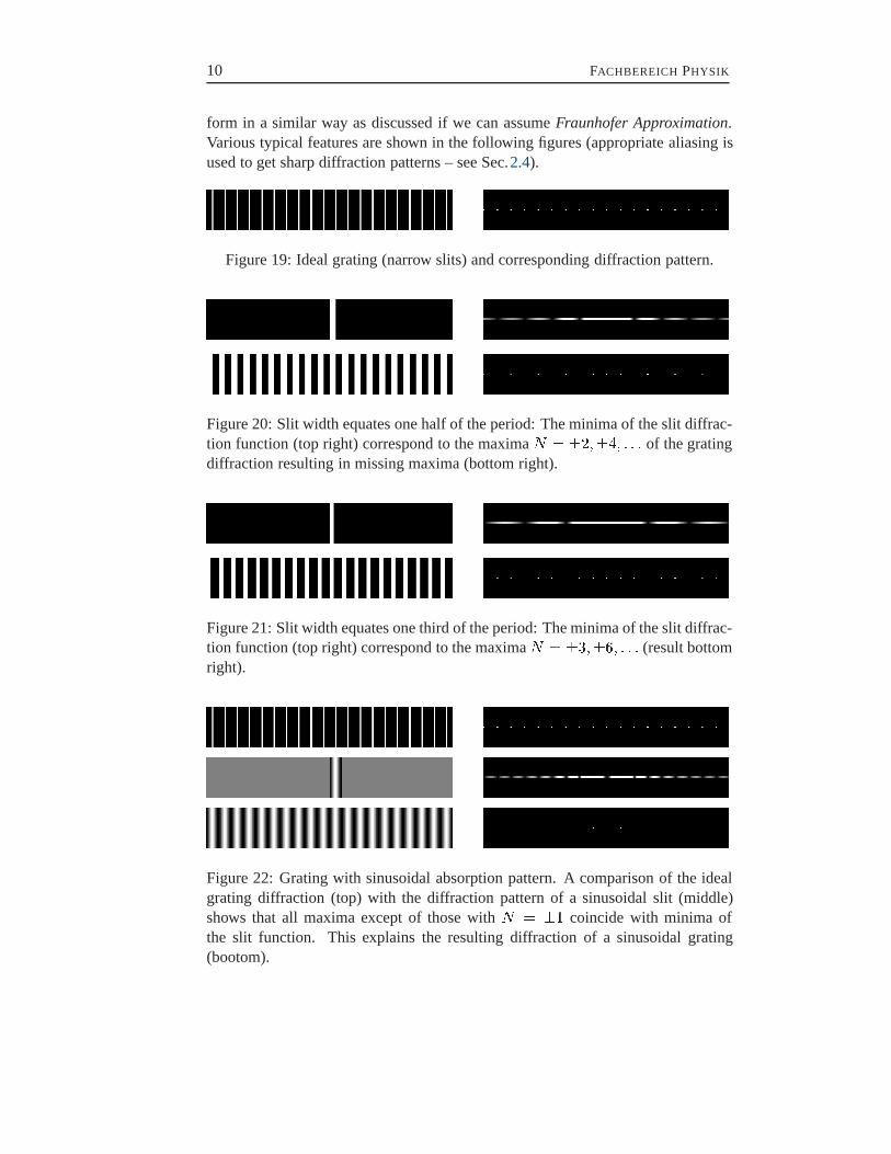
form in a similar way as discussed if we can assume Fraunhofer Approximation.Various typical features are shown in the following figures (appropriate aliasing isused to get sharp diffraction patterns – see Sec.2.4).

Figure 19: Ideal grating (narrow slits) and corresponding diffraction pattern.

Figure 20: Slit width equates one half of the period: The minima of the slit diffrac-tion function (top right) correspond to the maxima � � �� of the gratingdiffraction resulting in missing maxima (bottom right).

Figure 21: Slit width equates one third of the period: The minima of the slit diffrac-tion function (top right) correspond to the maxima � � �� (result bottomright).

Figure 22: Grating with sinusoidal absorption pattern. A comparison of the idealgrating diffraction (top) with the diffraction pattern of a sinusoidal slit (middle)shows that all maxima except of those with � � �� coincide with minima ofthe slit function. This explains the resulting diffraction of a sinusoidal grating(bootom).


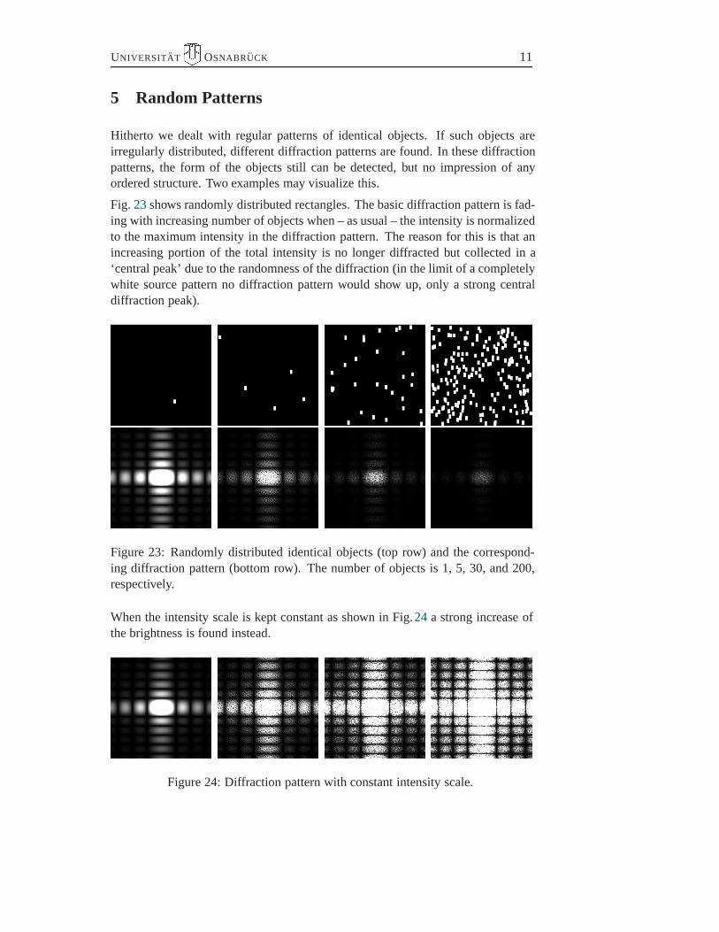
5 Random Patterns

Hitherto we dealt with regular patterns of identical objects. If such objects areirregularly distributed, different diffraction patterns are found. In these diffractionpatterns, the form of the objects still can be detected, but no impression of anyordered structure. Two examples may visualize this.

Fig. 23 shows randomly distributed rectangles. The basic diffraction pattern is fad-ing with increasing number of objects when – as usual – the intensity is normalizedto the maximum intensity in the diffraction pattern. The reason for this is that anincreasing portion of the total intensity is no longer diffracted but collected in a‘central peak’ due to the randomness of the diffraction (in the limit of a completelywhite source pattern no diffraction pattern would show up, only a strong centraldiffraction peak).

Figure 23: Randomly distributed identical objects (top row) and the correspond-ing diffraction pattern (bottom row). The number of objects is 1, 5, 30, and 200,respectively.

When the intensity scale is kept constant as shown in Fig.24 a strong increase ofthe brightness is found instead.

Figure 24: Diffraction pattern with constant intensity scale.


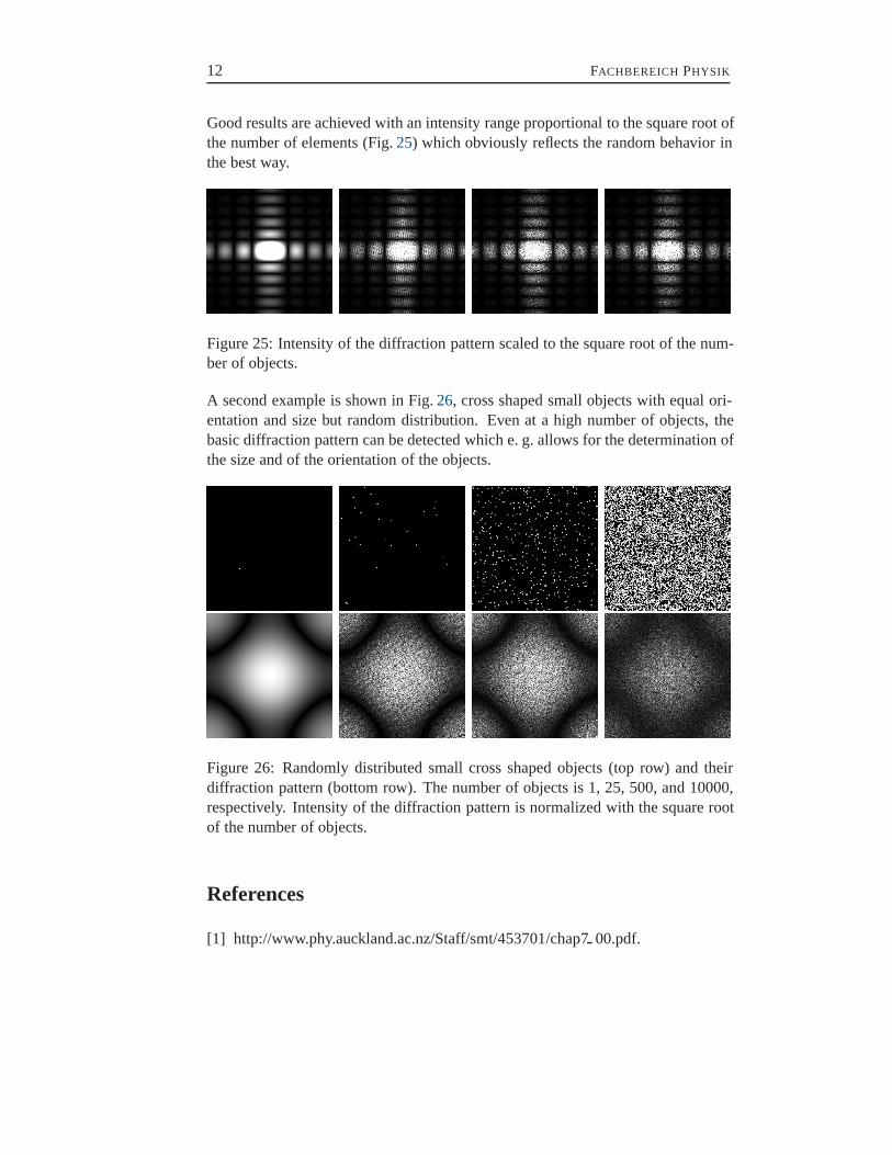
Good results are achieved with an intensity range proportional to the square root ofthe number of elements (Fig. 25) which obviously reflects the random behavior inthe best way.

Figure 25: Intensity of the diffraction pattern scaled to the square root of the num-ber of objects.

A second example is shown in Fig. 26, cross shaped small objects with equal ori-entation and size but random distribution. Even at a high number of objects, thebasic diffraction pattern can be detected which e. g. allows for the determination ofthe size and of the orientation of the objects.

Figure 26: Randomly distributed small cross shaped objects (top row) and theirdiffraction pattern (bottom row). The number of objects is 1, 25, 500, and 10000,respectively. Intensity of the diffraction pattern is normalized with the square rootof the number of objects.

References

[1] http://www.phy.auckland.ac.nz/Staff/smt/453701/chap7 00.pdf.

Fourier Optics in Examples - uni-osnabrueck.de · Fourier Optics in Examples FOURIER. ... (for a...

Documents

Transcript of Fourier Optics in Examples - uni-osnabrueck.de · Fourier Optics in Examples FOURIER. ... (for a...