Foundations of Statistical Inferencemarchini/bs2a/bs2a_4up.pdf · Foundations of Statistical...

Foundations of Statistical Inference

Jonathan Marchini

Department of StatisticsUniversity of Oxford

MT 2013

Jonathan Marchini (University of Oxford) BS2a MT 2013 1 / 282

Course arrangements

Lectures M.2 and Th.10 SPR1 weeks 1-8Classes Weeks 3-8 Friday 12-1, 2 × 4-5, 5-6 SPR1/2Hand in solutions by 12noon on Wednesday SPR1. Class Tutors :Jonathan Marchini, Charlotte GreenanNotes and Problem sheets will be available atwww.stats.ox.ac.uk\~marchini\bs2a.html

BooksGarthwaite, P. H., Jolliffe, I. T. and Jones, B. (2002) StatisticalInference, Oxford Science PublicationsLeonard, T., Hsu, J. S. (2005) Bayesian Methods, CambridgeUniversity Press.D. R. Cox (2006) Principals of Statistical Inference

This course builds on notes from Bob Griffiths and Geoff Nicholls


Part A StatisticsThe majority of the statistics that you have learned up to now fallsunder the philosophy of classical (or Frequentist) statistics. This theorymakes the assumption that we can randomly take repeated samples ofdata from the same population.You learned about three types of statistical inference

Point estimation (Maximum likelihood, bias, consistency,efficiency, information)Interval estimation(exact and approximate intervals using CLT)Hypothesis testing (Neyman-Pearson lemma, uniformly mostpowerful tests, generalised likelihood ratio tests)

You also had an introduction to Bayesian StatisticsPosterior inference (Posterior ∝ Likelihood × Prior)Interval estimation(credible intervals, HPD intervals)Priors(conjugate priors, improper priors, Jeffreys’ prior )Hypothesis testing (marginal likelihoods, Bayes Factors)


Frequentist inference

In BS2a we develop the theory of point estimation further.Are there families of distributions about which we can makegeneral statements? ⇒ Exponential families.How can we summarise all the information in a dataset about aparameter θ? ⇒ Sufficiency and the Factorization Theorem.What are limits of how well we can estimate a parameter θ?⇒Cramer-Rao inequality (and bound).How can we find good estimators of a parameter θ?⇒Rao-Blackwell Theorem and Lehmann-Scheffé Theorem.


www.stats.ox.ac.uk\ ~ marchini \ bs2a.html

Bayesian inferenceParameters are treated as random variables. Inference starts byspecifying a prior distribution on θ based on prior beliefs. Havingcollected some data we use Bayes’ Theorem to update our beliefs toobtain a posterior distribution.Quick Example Suppose I give a coin and tell you that it is bit biased.We might use a Beta(4,4) distribution to represent our beliefs about theθ. If we observe 30 heads and 10 tails we can use probability theory toinfer a posterior distribution for θ of Beta(34, 14).

0.0 0.2 0.4 0.6 0.8 1.0

0.0

0.5

1.0

1.5

2.0

Prior distribution

e

0.0 0.2 0.4 0.6 0.8 1.0

01

23

45

6

Posterior distribution

e


Computational techniques for Bayesian inference

It is not always possible to obtain an analytic solution when doingBayesian Inference, so we study approximate computationaltechniques in this course.These include

Markov chain Monte Carlo (MCMC) methodsApproximations to marginal likelihoods NEW

Variational ApproximationsLaplace approximationsBayesian Information Criterion (BIC)

The EM algorithm NEWuseful in Frequentist and Bayesian inference of missing dataproblems


Decision theory

Quick Example You have been exposed to a deadly virus. About 1/3of people who are exposed to the virus are infected by it, and all thoseinfected by it die unless they receive a vaccine. By the time anysymptoms of the virus show up, it is too late for the vaccine to work.You are offered a vaccine for £500. Do you take it or not?

The most likely scenario is that you don’t have the virus but basinga decision on this ignores the costs (or loss) associated with thedecisions. We would put a very high loss on dying!Decision theory allows us to formalise this problem.Closely connected to Bayesian ideas. Applicable to pointestimation and hypothesis testing. Inference is based onspecifying a number of possible actions we might take and a lossassociated with each action. The theory involves determining arule to make decisions using an overall measure of loss.


Notation

X ,Y ,Z Capital letters for random variables.x , y , z Lower case letters for realisations of random variables.EX (·) Expectation with respect to the random variable X .

φ = {φ1, . . . , φk} Sometimes we will use bold symbols to denote avector of parameters.


Lecture 1 - Exponential families


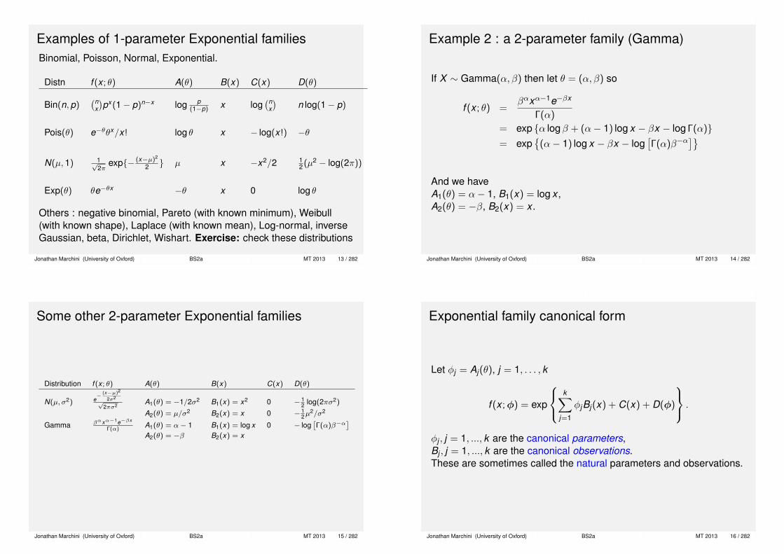
Parametric families

f (x ; θ), θ ∈ Θ, probability density of a random variable (rv) which couldbe discrete or continuous. θ can be 1-dimensional or of higherdimension. Equivalent notation:fθ(x),f (x | θ),f (x , θ).Likelihood L(θ; x) = f (x ; θ) and log-likelihood `(θ; x) = log(L).Examples1. Normal N(θ,1) : f (x ; θ) = 1√

2πe−

12 (x−θ)2

x ∈ R, θ ∈ R.

2. Poisson: f (x ; θ) = θx

x! e−θ, x = 0,1,2, . . . , θ > 0.

3. Regression:f (y ; θ) =

∏ni=1

1√2πσ

e−12 (yi−

∑pj=1 xijβj )

2, y ∈ Rn, σ > 0, β ∈ Rp. θ = {β, σ}.


Exponential families of distributions

Definition 1 GJJ 2.6, DRC 2.3A rv X belongs to a k -parameter exponential family if its probabilitydensity function (pdf) can be written as

f (x ; θ) = exp

k∑

j=1

Aj(θ)Bj(x) + C(x) + D(θ)

,

where x ∈ χ, θ ∈ Θ, A1(θ), . . . ,Ak (θ),D(θ) are functions of θ alone andB1(x),B2(x), . . . ,Bk (x),C(x) are well behaved functions of x alone.

Exponential families are widely used in practice - for example ingeneralised linear models (see BS1a).


Example 1 : Poisson

We want to put the Poisson distribution in the form (with k = 1)

f (x ; θ) = exp {A(θ)B(x) + C(x) + D(θ)} ,

e−θθx/x! = e−θ+x log θ−log x!

= exp {(log θ)x − log x!− θ}

So A(θ) = log θ,B(x) = x ,C(x) = − log x!,D(θ) = −θ.


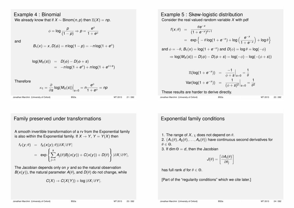
Examples of 1-parameter Exponential familiesBinomial, Poisson, Normal, Exponential.

Distn f (x ; θ) A(θ) B(x) C(x) D(θ)

Bin(n,p)(n

x

)px (1− p)n−x log p

(1−p) x log(n

x

)n log(1− p)

Pois(θ) e−θθx/x! log θ x − log(x!) −θ

N(µ,1) 1√2π

exp{− (x−µ)2

2 } µ x −x2/2 12 (µ2 − log(2π))

Exp(θ) θe−θx −θ x 0 log θ

Others : negative binomial, Pareto (with known minimum), Weibull(with known shape), Laplace (with known mean), Log-normal, inverseGaussian, beta, Dirichlet, Wishart. Exercise: check these distributions


Example 2 : a 2-parameter family (Gamma)

If X ∼ Gamma(α, β) then let θ = (α, β) so

f (x ; θ) =βαxα−1e−βx

Γ(α)

= exp {α logβ + (α− 1) log x − βx − log Γ(α)}= exp

{(α− 1) log x − βx − log

[Γ(α)β−α

]}And we haveA1(θ) = α− 1, B1(x) = log x ,A2(θ) = −β, B2(x) = x .


Some other 2-parameter Exponential families

Distribution f (x ; θ) A(θ) B(x) C(x) D(θ)

N(µ, σ2) e− (x−µ)2

2σ2√

2πσ2A1(θ) = −1/2σ2 B1(x) = x2 0 − 1

2 log(2πσ2)

A2(θ) = µ/σ2 B2(x) = x 0 − 12µ

2/σ2

Gamma βαxα−1e−βx

Γ(α)A1(θ) = α− 1 B1(x) = log x 0 − log

[Γ(α)β−α

]A2(θ) = −β B2(x) = x


Exponential family canonical form

Let φj = Aj(θ), j = 1, . . . , k

f (x ;φ) = exp

k∑

j=1

φjBj(x) + C(x) + D(φ)

.

φj , j = 1, ..., k are the canonical parameters,Bj , j = 1, ..., k are the canonical observations.These are sometimes called the natural parameters and observations.


Since ∫R

f (x ;φ)dx = 1

we have

∫R

exp

k∑

j=1

φjBj(x) + C(x) + D(φ)

dx = 1

exp{D(φ)}∫R

exp

k∑

j=1

φjBj(x) + C(x)

dx = 1

∫R

exp

k∑

j=1

φjBj(x) + C(x)

dx = exp{−D(φ)}


∫R

exp

k∑

j=1

φjBj(x) + C(x)

dx = exp{−D(φ)}

Differentiate with respect to φi .∫R

Bi (x) exp

k∑

j=1

φjBj (x) + C(x)

dx = − ∂

∂φiD(φ) exp{−D(φ)}

∫R

Bi (x) exp

k∑

j=1

φjBj (x) + C(x) + D(φ)

dx = − ∂

∂φiD(φ)

E[Bi (X )] = − ∂

∂φiD(φ)

Exercise Cov[Bi (X ),Bj (X )] = − ∂2

∂φi∂φjD(φ)

Exercise Var[Bi (X )] = − ∂2

∂φ2i

D(φ)


Example 3 : GammaWe already know that if X ∼ Gamma(α, β) the E(X ) = α

β andVar(X ) = α

β2 .

βαxα−1e−βx

Γ(α)= exp {−βx + (α− 1) log x + α logβ − log Γ(α)}

φ1 = −β, φ2 = α− 1, B1(x) = x , B2(x) = log x

D(φ) = α logβ − log Γ(α)

= (φ2 + 1) log(−φ1)− log Γ(φ2 + 1)

E[X ] = − ∂

∂φ1D(φ) = −(φ2 + 1)

φ1=α

β

Var[X ] = − ∂2

∂φ21

D(φ) = −(φ2 + 1)

φ21

=α

β2

Exercise: show E[log X ] = ψ0(α)− log(β) where ψ0 is the digammafunction, and Γ′(α) = Γ(α)ψ0(α).


Cumulant Generating FunctionIn a scalar canonical exponential family (k = 1)

EX [esB(X)] =

∫R

exp {(φ+ s)B(x) + C(x) + D(φ)}dx

= exp{D(φ)− D(φ+ s)}

If MB(X)(s) is the Moment Generating Function (mgf) for B(X ), then

log(MB(X)(s)) = D(φ)− D(φ+ s)

This is the cumulant generating function (defined as the log of the mgf)for the cumulants of B(X ) i.e.

log(MB(X)(s)) =∞∑

r=1

κr sr/r !

where κ1 = E(B(X )) and κ2 = V (B(X )) Exercise : prove thisJonathan Marchini (University of Oxford) BS2a MT 2013 20 / 282

Example 4 : BinomialWe already know that if X ∼ Binom(n,p) then E(X ) = np.

φ = logp

(1− p)⇒ p =

eφ

1 + eφ

andB1(x) = x ,D(φ) = n log(1− p) = −n log(1 + eφ)

log(MX (s)) = D(φ)− D(φ + s)

= −n log(1 + eφ) + n log(1 + eφ+s)

Therefore

κ1 =∂

∂slog(MX (s))

∣∣∣s=0

= neφ

1 + eφ= np


Example 5 : Skew-logistic distributionConsider the real valued random variable X with pdf

f (x ; θ) =θe−x

(1 + e−x )θ+1

= exp{− θ log(1 + e−x ) + log

( e−x

1 + e−x

)+ log θ

}and φ = −θ, B1(x) = log(1 + e−x ) and D(φ) = log θ = log(−φ)

⇒ log(MX (s)) = D(φ)− D(φ + s) = log(−φ)− log(−(φ+ s))

E(log(1 + e−x )) =−1φ+ s

∣∣∣s=0

=1θ

Var(log(1 + e−x )) =1

(φ+ s)2

∣∣∣s=0

=1θ2

These results are harder to derive directly.Jonathan Marchini (University of Oxford) BS2a MT 2013 22 / 282

Family preserved under transformations

A smooth invertible transformation of a rv from the Exponential familyis also within the Exponential family. If X → Y , Y = Y (X ) then

fY (y ; θ) = fX (x(y); θ)|∂X/∂Y |

= exp

k∑

j=1

Aj(θ)Bj(x(y)) + C(x(y)) + D(θ)

|∂X/∂Y |,

The Jacobian depends only on y and so the natural observationB(x(y)), the natural parameter A(θ), and D(θ) do not change, while

C(X )→ C(X (Y )) + log |∂X/∂Y |.


Exponential family conditions

1. The range of X , χ does not depend on θ.2.(A1(θ),A2(θ), . . . ,Ak (θ)

)have continuous second derivatives for

θ ∈ Θ.3. If dim Θ = d , then the Jacobian

J(θ) =

[∂Ai(θ)

∂θj

]has full rank d for θ ∈ Θ.

[Part of the “regularity conditions” which we cite later.]


The family is minimal if no linear combination exists such that

λ0 + λ1B1(x) + · · ·+ λkBk (x) = 0

for all x ∈ χ.The dimension of the family is defined to be d , the rank of J(θ).A minimal exponential family is said to be curved when d < k andlinear when d = k . We refer to a (k ,d) curved exponential family.Example 6 (X1,X2) independent, normal, unit variance, means(θ, c/θ), c known.

log f (x ; θ) = x1θ + cx2/θ − θ2/2− c2θ−2/2 + ...

is a (2,1) curved exponential family.


Linear relations among A’s do not generate curvature

Take a k -parameter exponential family and impose A1 = aA2 + b forconstants a and b.

k∑i=1

AiBi + C + D =k∑

i=3

AiBi + A2(aB1 + B2) + (C + bB1) + D

This gives a k − 1 parameter EF, not a (k , k − 1)-CEF.


Examples not in an exponential family

1 Uniform on [0, θ], θ > 0.

f (x ; θ) =1θ, x ∈ [0, θ] θ > 0

2 The Cauchy distribution

f (x ; θ) = [π(1 + (x − θ)2)]−1, x ∈ R

Other examples include the F-distribution, hypergeometricdistribution and logistic distribution.


Lecture 2 - Sufficiency, Factorization Theorem, Minimal sufficiency


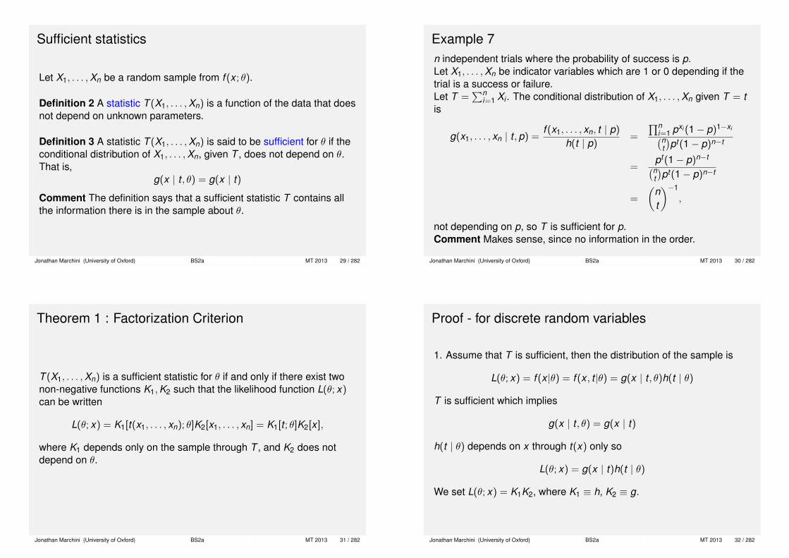
Sufficient statistics

Let X1, . . . ,Xn be a random sample from f (x ; θ).

Definition 2 A statistic T (X1, . . . ,Xn) is a function of the data that doesnot depend on unknown parameters.

Definition 3 A statistic T (X1, . . . ,Xn) is said to be sufficient for θ if theconditional distribution of X1, . . . ,Xn, given T , does not depend on θ.That is,

g(x | t , θ) = g(x | t)

Comment The definition says that a sufficient statistic T contains allthe information there is in the sample about θ.


Example 7n independent trials where the probability of success is p.Let X1, . . . ,Xn be indicator variables which are 1 or 0 depending if thetrial is a success or failure.Let T =

∑ni=1 Xi . The conditional distribution of X1, . . . ,Xn given T = t

is

g(x1, . . . , xn | t ,p) =f (x1, . . . , xn, t | p)

h(t | p)=

∏ni=1 pxi (1− p)1−xi(n

t

)pt (1− p)n−t

=pt (1− p)n−t(nt

)pt (1− p)n−t

=

(nt

)−1

,

not depending on p, so T is sufficient for p.Comment Makes sense, since no information in the order.


Theorem 1 : Factorization Criterion

T (X1, . . . ,Xn) is a sufficient statistic for θ if and only if there exist twonon-negative functions K1,K2 such that the likelihood function L(θ; x)can be written

L(θ; x) = K1[t(x1, . . . , xn); θ]K2[x1, . . . , xn] = K1[t ; θ]K2[x ],

where K1 depends only on the sample through T , and K2 does notdepend on θ.


Proof - for discrete random variables

1. Assume that T is sufficient, then the distribution of the sample is

L(θ; x) = f (x |θ) = f (x , t |θ) = g(x | t , θ)h(t | θ)

T is sufficient which implies

g(x | t , θ) = g(x | t)

h(t | θ) depends on x through t(x) only so

L(θ; x) = g(x | t)h(t | θ)

We set L(θ; x) = K1K2, where K1 ≡ h, K2 ≡ g.


2. Suppose L(θ; x) = f (x | θ) = K1[t ; θ]K2[x ].Then

h(t | θ) =∑

{x :T (x)=t}

f (x , t | θ) =∑

{x :T (x)=t}

L(θ; x)

= K1[t ; θ]∑

{x :T (x)=t}

K2(x).

Thus

g(x | t , θ) =f (x , t | θ)

h(t | θ)=

L(θ; x)

h(t | θ)=

K2[x ]∑{x :T (x)=t} K2(x)

,

not depending on θ. (K1 cancels out in numerator and denominator.)


Minimal sufficiencyIn general, we can envisage a sequence of functionsT1(X ),T2(X ),T3(X ), . . . such that Tj(X ) is a function of Tj−1(X ) (j ≥ 2)where moving along the sequence gains progressive reductions ofdata, and if Tj(X ) is sufficient for θ, then so is Ti(X ) i < j . Typicallythere will be a last member Tk (X ) that is sufficient, with Ti(X ) notsufficient for i > k . Then Tk (X ) is minimal sufficient

Example 7 (cont.) Consider n = 3 Bernoulli trials1 T1(X ) = (X1,X2,X3) (the individual sequences of trials)2 T2(X ) = (X1,

∑3i=1 Xi) (the 1st random variable and the total sum).

3 T3(X ) =∑3

i=1 Xi (the total sum)4 T4(X ) = I(T3(X ) = 0) (I is indicator function; Exercise Prove T4

not sufficient)

Definition 4 A statistic is minimal sufficient if it can be expressed as afunction of every other sufficient statistic.


Example 7 (cont.) : Minimal sufficiencyn Bernoulli trials with T =

∑ni=1 Xi . Suppose T above is not minimal

sufficient but another statistic U is MS.Then U can be given as afunction of T (and not vis versa or T is MS) and there exist t1 6= t2values of T so that U(t1) = U(t2)(ie T → U is many to one so U → Tis not a function, and we assume for the moment no other t makeU(t) = U(t1)).The event U = u is the event T ∈ {t1, t2}. Let x1, ...xncontain t1 successes. Then

g(x1, . . . , xn|u,p) = g(x1, . . . , xn|t1,p)P(t1|u,p)

= g(x1, . . . , xn|t1)P(T = t1|T ∈ {t1, t2})

=pt1(1− p)n−t1(n

t1

)pt1(1− p)n−t1 +

(nt2

)pt2(1− p)n−t2

which depends on p, so U is not sufficient, a contradiction, and henceT must be MS (similar reasoning for multiple ti ).


Minimal sufficiency and partitions of the sample space

Intuitively, a minimal sufficient statistic most efficiently captures allpossible information about the parameter θ.Any statistic T (X ) partitions the sample space into subsets and ineach subset T (X ) has constant value.Minimal sufficient statistics correspond to the coarsest possiblepartition of the sample space.In the example of n = 3 Bernoulli trials consider the following 4statistics and the partitions they induce.


TTT

TTH

THT

THH

HTT

HHT

HTH

HHH

TTT

TTH

THT

THH

HTT

HHT

HTH

HHH

TTT

TTH

THT

THH

HTT

HHT

HTH

HHH

TTT

TTH

THT

THH

HTT

HHT

HTH

HHH

T1(X) = X1,X2,X3( )

T3(X) = Xii=1

3

∑ T4 (X) = I T3(X) = 0( )

T2 (X) = X1, Xii=1

3

∑⎛⎝⎜

⎞⎠⎟


Lemma 1 : Lehmann-Scheffé partitions

Consider the partition of the sample space defined by putting x and yinto the same class of the partition if and only if

L(θ; y)/L(θ; x) = f (y | θ)/f (x | θ) = m(x , y).

Then any statistic corresponding to this partition is minimal sufficient.

Comment This Lemma tells us how to define partitions thatcorrespond to minimal sufficient statistics. It says that ratios oflikelihoods of two values x and y in the same partition (and hencesame statistic value) should not depend on θ.


Proof (for discrete RVs)

1. Sufficiency.Suppose T is such a statistic

g(x |t , θ) =f (x | θ)

f (t | θ)=

f (x | θ)∑y∈τ f (y | θ)

, τ = {y : T (y) = t}

=f (x | θ)∑

y∈τ f (x | θ)m(x , y)

=[∑

y∈τm(x , y)

]−1

which does not depend on θ. Hence the partition D is sufficient.


2. Minimal sufficiency.Now suppose U is any other sufficient statistic and that U(x) = U(y)for some pair of values (x , y). If we can show that U(x) = U(y) impliesT (x) = T (y), then the Lehmann-Scheffé partition induced by Tincludes the partition based on any other sufficient statistic.In otherwords, T is a function of every other sufficient statistic, and so must beminimal sufficient.Since U is sufficient we have

L(θ; y)

L(θ; x)=

K1[u(y); θ]K2[y ]

K1[u(x); θ]K2[x ]=

K2[y ]

K2[x ]

which does not depend on θ. So the statistic U produces a partition atleast as fine as that induced by T , and the result is proved.


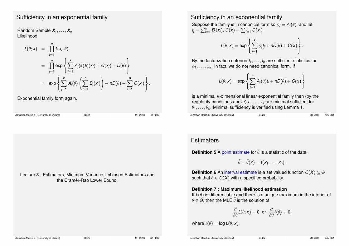
Sufficiency in an exponential family

Random Sample X1, . . . ,XnLikelihood

L(θ; x) =n∏

i=1

f (xi ; θ)

=n∏

i=1

exp

k∑

j=1

Aj(θ)Bj(xi) + C(xi) + D(θ)

= exp

k∑

j=1

Aj(θ)

(n∑

i=1

Bj(xi)

)+ nD(θ) +

n∑i=1

C(xi)

.

Exponential family form again.


Sufficiency in an exponential familySuppose the family is in canonical form so φj = Aj(θ), and lettj =

∑ni=1 Bj(xi), C(x) =

∑ni=1 C(xi).

L(θ; x) = exp

k∑

j=1

φj tj + nD(θ) + C(x)

.

By the factorization criterion t1, . . . , tk are sufficient statistics forφ1, . . . , φk . In fact, we do not need canonical form. If

L(θ; x) = exp

k∑

j=1

Aj(θ)tj + nD(θ) + C(x)

is a minimal k -dimensional linear exponential family then (by theregularity conditions above) t1, . . . , tk are minimal sufficient forθ1, . . . , θk . Minimal sufficiency is verified using Lemma 1.


Lecture 3 - Estimators, Minimum Variance Unbiased Estimators andthe Cramér-Rao Lower Bound.


Estimators

Definition 5 A point estimate for θ is a statistic of the data.

θ = θ(x) = t(x1, . . . , xn).

Definition 6 An interval estimate is a set valued function C(X ) ⊆ Θsuch that θ ∈ C(X ) with a specified probability.

Definition 7 : Maximum likelihood estimationIf L(θ) is differentiable and there is a unique maximum in the interior ofθ ∈ Θ, then the MLE θ is the solution of

∂

∂θL(θ; x) = 0 or

∂

∂θ`(θ) = 0,

where `(θ) = log L(θ; x).


Lemma 2 : MLEs and exponential families

Consider a k -dimensional exponential family in canonical form

L(θ; x) = exp

k∑

j=1

φj

(n∑

i=1

Bj(xi)

)+ nD(φ) +

n∑i=1

C(xi)

.

Let Tj(X ) =∑n

i=1 Bj(Xi), j = 1, . . . , k . If the realized data are X = x ,then the statistics evaluated on the data are Tj(x) = tj .The MLEs of φ1, . . . , φk are the solution of

tj = EX (Tj), j = 1, . . . , k .

i.e. set the expected values of the sufficient statistics equal to theirrealised values and solve for φj . [If the family is not in canonical form,there is a similar slightly more complicated matrix equation]


Proof

` = log L = const +k∑

j=1

φj tj + nD(φ)

⇒ ∂

∂φj` = tj + n

∂

∂φjD(φ)

However, since EX [Bi(X )] = − ∂∂φi

D(φ) and Tj(X ) =∑n

i=1 Bj(Xi) weknow that

EX [Tj ] = −n∂

∂φjD(φ), so

∂

∂φj` = tj − EX (Tj) = 0

is equivalent to tj = EX (Tj).


Bias, Variance, Mean Squared Error

Tn = T (X1, . . . ,Xn) is a statistic.Definition 8 Tn is unbiased for a function g(θ) if

EX (Tn) =

∫χ

tn(x)f (x ; θ)dx = g(θ), for all θ ∈ Θ.

Definition 9 The bias of an estimator Tn is bias(Tn) = EX [Tn − g(θ)]Definition 10 Tn is a consistent estimator if

∀ε > 0,P(|Tn − θ| > ε)→ 0 as n→∞.Definition 11 The Mean Squared Error (MSE) of Tn is

MSE(Tn) = EX [Tn − g(θ)]2 = VX (Tn) + [bias(Tn)]2

Example 10 N(µ, σ2). µ = X and S2 = (n − 1)−1∑ni=1(Xi − X

)2 areunbiased estimates of µ and σ2.


Minimum Variance Unbiased Estimators (MVUE)

If we want to find a good estimator then one obvious strategy is totry to find estimators that minimise MSE. This is often difficult.For example, if we choose the estimator θ = θ0 then this hasMSE=0 when θ = θ0, so no other estimator can be uniformly bestunless it has zero MSE everywhere.If we restrict attention to unbiased estimators then the situationbecomes more tractable. In this case, MSE reduces to thevariance of the estimator and we can focus on minimising thevariance of estimators. That is, we search for minimum varianceunbiased estimators (MVUE).


Theorem 2 : Cramér-Rao inequality (and bound).If θ is an unbiased estimator of θ, then subject to certain regularityconditions on f (x ; θ), we have

Var(θ) ≥ I−1θ .

where Iθ, the Fisher information, is given by

Iθ = −E[∂2

∂θ2 `(θ)

]Comment This bound tells us the minimum possible variance. If anestimator achieves the bound then it is MVUE. There is no guaranteethat the bound will be attainable. In many cases it is attainableasymptotically. Intuitively, the more ‘information’ we have about θ, thelarger Iθ will be and lowest possible variance of the estimator will besmaller.


Regularity conditions for CRLB

We will not be concerned with the details of the required regularityconditions.The main reason they are needed is to ensure that it is ok tointerchange integration and differentiation during parts of theproof.One condition that is often easy to check is that the range of the rvX must not depend on θ. So for example, the result can not beapplied when working with the uniform distribution U[0, θ] and wewish to estimate θ.


In order to prove the CRLB we will need to use a few results.

Proposition 1 : Variance-Covariance inequalityLet U and V be scalar rv. Then

cov(U,V )2 ≤ var(U)var(V )

with equality if and only if U = aV + b for constants and a 6= 0.


The Fisher Information Iθ, which is used in the Cramér-Rao lowerbound, can be expressed in two different forms.

Lemma 3 Under regularity conditions

Iθ = −E[∂2

∂θ2 `(θ)

]= E

[(∂`

∂θ

)2]

= Var[S(X ; θ)],

where the score function s(x ; θ) is defined as

s(x ; θ) =∂

∂θ`(θ) =

f ′(x ; θ)

f (x ; θ)


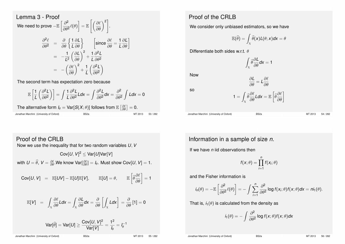
Lemma 3 - ProofWe need to prove −E

[∂2

∂θ2 `(θ)

]= E

[(∂`

∂θ

)2]

.

∂2`

∂θ2 =∂

∂θ

{1L∂L∂θ

} [since

∂`

∂θ=

1L∂L∂θ

]= − 1

L2

(∂L∂θ

)2

+1L∂2L∂θ2

= −(∂`

∂θ

)2

+1L

(∂2L∂θ2

)The second term has expectation zero because

E[

1L

(∂2L∂θ2

)]=

∫1L∂2L∂θ2 Ldx =

∫∂2L∂θ2 dx =

∂2

∂θ2

∫Ldx = 0

The alternative form Iθ = Var[S(X ; θ)] follows from E[∂`∂θ

]= 0.


Proof of the CRLB

We consider only unbiased estimators, so we have

E(θ) =

∫χθ(x)L(θ; x)dx = θ

Differentiate both sides w.r.t. θ∫χθ∂L∂θ

dx = 1

Now∂L∂θ

= L∂`

∂θso

1 =

∫χθ∂`

∂θLdx = E

[θ∂`

∂θ

]


Proof of the CRLBNow we use the inequality that for two random variables U,V

Cov[U,V ]2 ≤ Var[U]Var[V ]

with U = θ, V = ∂`∂θ .We know Var[ ∂`∂θ ] = Iθ. Must show Cov[U,V ] = 1.

Cov[U,V ] = E[UV ]− E[U]E[V ], E[U] = θ, E[θ∂`

∂θ

]= 1

E[V ] =

∫χ

∂`

∂θLdx =

∫χ

∂L∂θ

dx =∂

∂θ

[∫χ

Ldx]

=∂

∂θ[1] = 0

Var[θ] = Var[U] ≥ Cov[U,V ]2

Var[V ]=

12

Iθ= I−1

θ


Information in a sample of size n.

If we have n iid observations then

f (x ; θ) =n∏

i=1

f (xi ; θ)

and the Fisher information is

in(θ) = −E[∂2

∂θ2 `(θ)

]= −

∫ n∑i=1

∂2

∂θ2 log f (xi ; θ)f (x ; θ)dx = ni1(θ).

That is, i1(θ) is calculated from the density as

i1(θ) = −∫

∂2

∂θ2 log f (x ; θ)f (x ; θ)dx


Lecture 4 - Consequences of the Cramér-Rao Lower Bound.Searching for a MVUE. Rao-Blackwell Theorem, Lehmann-Scheffé

Theorem.


Question Under what conditions will we be able to attain theCramér-Rao bound and find a MVUE?

Corollary 1 There exists an unbiased estimator θ which attains the CRlower bound (under regularity conditions) if and only if

∂`

∂θ= Iθ(θ − θ)

Proof In the CR proof

Cov[U,V ]2 ≤ Var[U]Var[V ]

and the lower bound is attained if and only equality is achieved. IfU = θ,V = ∂`

∂θ , the equality occurs when ∂`∂θ = c + d θ, where c,d are

constants. E[V ] = 0 so c = −dθ and ∂`∂θ = d(θ − θ).


Multiply by ∂`/∂θ and take expectations.

E

[(∂`

∂θ

)2]

= dE[∂`

∂θθ

]− dθE

[∂`

∂θ

]= d × 1− 0

The LHS is Iθ so we have d = Iθ and

∂`

∂θ= Iθ(θ − θ)


Question What is the relationship between the CRLB and exponentialfamilies?

Corollary 2 If there exists an unbiased estimator θ(X ) which attainsthe CR lower bound (under regularity conditions) it follows that X mustbe in an exponential familyProof Taking n = 1

∂ log f (x ; θ)

∂θ=∂`

∂θ= Iθ(θ − θ)

andlog f (x ; θ) = θA(θ) + D(θ) + C(x)

which is an exponential family form. The constant of integration C(x) isa function of x .


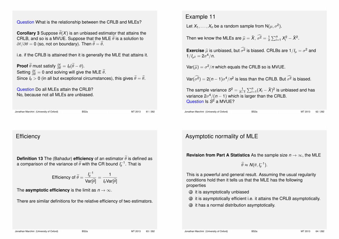
Question What is the relationship between the CRLB and MLEs?

Corollary 3 Suppose θ(X ) is an unbiased estimator that attains theCRLB, and so is a MVUE. Suppose that the MLE θ is a solution to∂`/∂θ = 0 (so, not on boundary). Then θ = θ.

i.e. if the CRLB is attained then it is generally the MLE that attains it.

Proof θ must satisfy ∂`∂θ = Iθ(θ − θ).

Setting ∂`∂θ = 0 and solving will give the MLE θ.

Since Iθ > 0 (in all but exceptional circumstances), this gives θ = θ.

Question Do all MLEs attain the CRLB?No, because not all MLEs are unbiased.


Example 11

Let X1, . . . ,Xn be a random sample from N(µ, σ2).

Then we know the MLEs are µ = X , σ2 = 1n∑n

i=1 X 2i − X 2.

Exercise µ is unbiased, but σ2 is biased. CRLBs are 1/Iµ = σ2 and1/Iσ2 = 2σ4/n.

Var(µ) = σ2/n which equals the CRLB so is MVUE.

Var(σ2) = 2(n − 1)σ4/n2 is less than the CRLB. But σ2 is biased.

The sample variance S2 = 1n−1

∑ni=1(Xi − X )2 is unbiased and has

variance 2σ4/(n − 1) which is larger than the CRLB.Question Is S2 a MVUE?


Efficiency

Definition 13 The (Bahadur) efficiency of an estimator θ is defined asa comparison of the variance of θ with the CR bound I−1

θ . That is

Efficiency of θ =I−1θ

Var[θ]=

1

IθVar[θ]

The asymptotic efficiency is the limit as n→∞.

There are similar definitions for the relative efficiency of two estimators.


Asymptotic normality of MLE

Revision from Part A Statistics As the sample size n→∞, the MLE

θ ≈ N(θ, I−1θ ).

This is a powerful and general result. Assuming the usual regularityconditions hold then it tells us that the MLE has the followingproperties

1 it is asymptotically unbiased2 it is asymptotically efficient i.e. it attains the CRLB asymptotically.3 it has a normal distribution asymptotically.


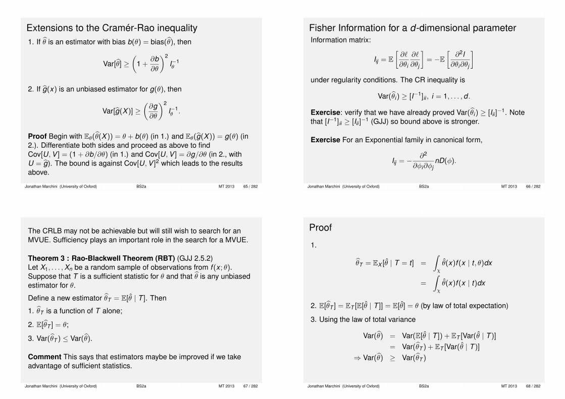
Extensions to the Cramér-Rao inequality1. If θ is an estimator with bias b(θ) = bias(θ), then

Var[θ] ≥(

1 +∂b∂θ

)2

I−1θ

2. If g(x) is an unbiased estimator for g(θ), then

Var[g(X )] ≥(∂g∂θ

)2

I−1θ .

Proof Begin with Eθ(θ(X )) = θ + b(θ) (in 1.) and Eθ(g(X )) = g(θ) (in2.). Differentiate both sides and proceed as above to findCov[U,V ] = (1 + ∂b/∂θ) (in 1.) and Cov[U,V ] = ∂g/∂θ (in 2., withU = g). The bound is against Cov[U,V ]2 which leads to the resultsabove.


Fisher Information for a d-dimensional parameterInformation matrix:

Iij = E[∂`

∂θi

∂`

∂θj

]= −E

[∂2l

∂θi∂θj

]under regularity conditions. The CR inequality is

Var(θi) ≥ [I−1]ii , i = 1, . . . ,d .

Exercise: verify that we have already proved Var(θi) ≥ [Iii ]−1. Notethat [I−1]ii ≥ [Iii ]−1 (GJJ) so bound above is stronger.

Exercise For an Exponential family in canonical form,

Iij = − ∂2

∂φi∂φjnD(φ).


The CRLB may not be achievable but will still wish to search for anMVUE. Sufficiency plays an important role in the search for a MVUE.

Theorem 3 : Rao-Blackwell Theorem (RBT) (GJJ 2.5.2)Let X1, . . . ,Xn be a random sample of observations from f (x ; θ).Suppose that T is a sufficient statistic for θ and that θ is any unbiasedestimator for θ.

Define a new estimator θT = E[θ | T ]. Then

1. θT is a function of T alone;

2. E[θT ] = θ;

3. Var(θT ) ≤ Var(θ).

Comment This says that estimators maybe be improved if we takeadvantage of sufficient statistics.


Proof

1.

θT = EX [θ | T = t ] =

∫χθ(x)f (x | t , θ)dx

=

∫χθ(x)f (x | t)dx

2. E[θT ] = ET [E[θ | T ]] = E[θ] = θ (by law of total expectation)

3. Using the law of total variance

Var(θ) = Var(E[θ | T ]) + ET [Var(θ | T )]

= Var(θT ) + ET [Var(θ | T )]

⇒ Var(θ) ≥ Var(θT )


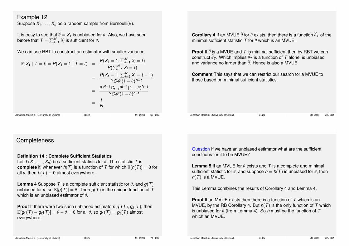
Example 12Suppose X1, . . . ,Xn be a random sample from Bernoulli(θ).

It is easy to see that θ = X1 is unbiased for θ. Also, we have seenbefore that T =

∑Ni=1 Xi is sufficient for θ.

We can use RBT to construct an estimator with smaller variance

E[X1 | T = t ] = P(X1 = 1 | T = t) =P(X1 = 1,

∑Ni=1 Xi = t)

P(∑N

i=1 Xi = t)

=P(X1 = 1,

∑Ni=2 Xi = t − 1)

NCtθt (1− θ)N−t

=θ.N−1Ct−1θ

t−1(1− θ)N−t

NCtθt (1− θ)n−t

=tN


Corollary 4 If an MVUE θ for θ exists, then there is a function θT of theminimal sufficient statistic T for θ which is an MVUE.

Proof If θ is a MVUE and T is minimal sufficient then by RBT we canconstruct θT . Which implies θT is a function of T alone, is unbiasedand variance no larger than θ. Hence is also a MVUE.

Comment This says that we can restrict our search for a MVUE tothose based on minimal sufficient statistics.


Completeness

Definition 14 : Complete Sufficient StatisticsLet T (X1, . . . ,Xn) be a sufficient statistic for θ. The statistic T iscomplete if, whenever h(T ) is a function of T for which E[h(T )] = 0 forall θ, then h(T ) ≡ 0 almost everywhere.

Lemma 4 Suppose T is a complete sufficient statistic for θ, and g(T )unbiased for θ, so E[g(T )] = θ. Then g(T ) is the unique function of Twhich is an unbiased estimator of θ.

Proof If there were two such unbiased estimators g1(T ),g2(T ), thenE[g1(T )− g2(T )] = θ − θ = 0 for all θ, so g1(T ) = g2(T ) almosteverywhere.


Question If we have an unbiased estimator what are the sufficientconditions for it to be MVUE?

Lemma 5 If an MVUE for θ exists and T is a complete and minimalsufficient statistic for θ, and suppose h = h(T ) is unbiased for θ, thenh(T ) is a MVUE.

This Lemma combines the results of Corollary 4 and Lemma 4.

Proof If an MVUE exists then there is a function of T which is anMVUE, by the RB Corollary 4. But h(T ) is the only function of T whichis unbiased for θ (from Lemma 4). So h must be the function of Twhich an MVUE.


Question Finally, how can we construct a MVUE?

Theorem 4 : Lehmann-Scheffé theorem Let T be a completesufficient statistic for θ, and let θ be an unbiased estimator for θ, thenthe unbiased estimator θT = E[θ | T ] has the smallest variance amongall unbiased estimators of θ. That is,

Var(θT ) ≤ Var(θ)

for all unbiased estimators θ.

Comment This theorem says that if we can find any unbiasedestimator and a complete sufficient statistic T then we can construct aMVUE.


Proof

Suppose θ exists with Var(θ) < Var(θT ).

Then by RBT we can construct θT = E[θ | T ] such that

Var(θT ) ≤ Var(θ) < Var(θT )

But θT and θT are both unbiased and T is complete, so by Lemma 4we have θT = θT and

Var(θT ) = Var(θT )

which is a contradiction.


Lemma 6 : Complete Sufficiency in EFsIf the rv X has a distribution belonging to a k -parameter exponentialfamily, then under the usual regularity conditions, the statistic

( n∑i=1

B1(Xi),n∑

i=1

B2(Xi), . . . ,n∑

i=1

Bk (Xi))

which we already know is minimal sufficient, is complete.

Comment We showed before that MLEs for exponential families werefunctions of this same statistic.

Therefore, for a member of an exponential family if the MLE isunbiased (note : not all MLEs are unbiased), then by Lemma 5, theMLE will be MVUE. If there is an unbiased estimator that attains theCRLB then, by Corollary 3, the MLE will attain the CRLB.


Example 13Let X1, . . . ,Xn be a random sample from N(µ, σ2).

Then we know the MLEs are µ = X , σ2 = 1n∑n

i=1 X 2i − X 2.

µ is unbiased, but σ2 is biased.

Exercise The minimal sufficient complete statistic is(∑ni=1 Xi ,

∑ni=1 X 2

i

).

So µ is MVUE and attains the CRLB with variance σ2/n.

The sample variance S2 = 1n−1

∑ni=1(Xi − X )2 is unbiased and is a

function of the minimal sufficient complete statistic so is MVUE withvariance 2σ4/(n − 1) which is larger than the CRLB of 2σ4/n.


Lecture 5 - Method of Moments


Method of momentsGenerate estimators by equating observed statistics with theirexpected values

E{t(X1, . . . ,Xn)} = t(x1, . . . , xn).

Comment Simple, easy to use. Often have good properties, but notguaranteed. Can provide good starting point for an iterative method forfinding MLEs.

Example 14 Uniform iid sample X = (X1,X2, ...,Xn) on (0, θ).

L(θ; x) = f (x ; θ) = θ−n, 0 < x1, . . . , xn < θ.

Let X(n) = maxi Xi . In this case the moment relation

E[X(n)

]= x(n)

leads to an unbiased sufficient statistic, θ = n+1n X(n).


Method of moments

The distribution of X(n) = maxi Xi is obtained from the CDF

P(X(n) ≤ y) =(yθ

)n

(the probability all iid Xi fall in (0, y)) so

fX(n)(y ; θ) =

nyn−1

θn , 0 < y < θ

andE[X(n)

]=

nn + 1

θ, so θ =n + 1

nX(n)

is unbiased.


Now check θ is sufficient.

The distribution of X | X(n) = y is

f (x |X(n) = y ; θ) =f (x ; θ)

fX(n)(y ; θ)

=1

nyn−1

which does not depend on θ.

θ is minimal sufficient since

L(θ; x)

L(θ; y)=θ−nI[x(n) < θ]

θ−nI[y(n) < θ]

does not depend on θ if x(n) = y(n) i.e. θ forms a Lehmann-Scheffépartition.


Finally, we can show that θ = θ(X(n)) is complete.

If E[θ] = 0 for all θ > 0 then∫ θ

0h(θ(y))

nyn−1

θn dy = 0

for all θ > 0 and hence ∫ θ

0h(θ(y))yn−1dy = 0.

Differentiate wrt θ (using the Leibniz integral rule), and concludeh(θ) = 0 identically for all X . It follows that θ is the unique unbiasedestimator based on X(n).

Since θ is minimal sufficient, if a MVUE exists, it equals θ (Corollary 4).

We can’t use the CRB to show a MVUE exists, as the problem isnon-regular.


Exercise `(θ; x) = −n log(θ) so

E

[(∂`

∂θ

)2]

= n2/θ2

and the CRB would be Var(θ) ≥ θ2/n2.

However, you can check (using fX(n)(y ; θ) above) that

Var(θ) =θ2

n(n + 1)

which is smaller than θ2/n2 for any n ≥ 1.

This is not a contradiction, as f (x ; θ) doesn’t satisfy the regularityconditions (limits of x depend on θ).


We can find the MLE in this example

θ = X(n)

but this estimator is1 biased and the Uniform density does not satisfy the regularity

condition needed for CRLB so it does not apply.2 does not satisfy ∂`/∂θ = 0, so even if the CRLB did apply we

cannot make the link between the MLE and the lower bound.


Example 15A sample from N(µ, σ2). The moment relations

E

[n∑

i=1

Xi

]= nµ, E

[n∑

i=1

X 2i

]= n(µ2 + σ2)

lead to the estimating equations

µ = X , µ2 + σ2 = n−1n∑

i=1

X 2i .

We have seen that these are just the equations for the MLE’s in this2-dimensional exponential linear family, and solve to give the MLE

σ2 = n−1n∑

i=1

(Xi − X )2.


Example 16A sample from Pois(λ). We have two possible moment relations

E

[1n

n∑i=1

Xi

]= λ, ⇒ λ1 =

1n

n∑i=1

Xi

E

[1n

n∑i=1

(Xi − X )2

]= λ, ⇒ λ2 =

1n

n∑i=1

(Xi − X )2

For a sample of size n we haveA(λ) = logλ, B(x) =

∑ni=1 xi , C(x) = − log(

∏ni=1 xi !), D(λ) = −nλ

By Lemma 6 we have that B(x) =∑n

i=1 xi is a sufficient completestatistic. Thus by the Lehmann-Scheffé Theorem we have thatarithmetic mean λ1 is MVUE. λ2 is not a function of B(x).

Exercise Show that λ1 attains the CRLB.Jonathan Marchini (University of Oxford) BS2a MT 2013 85 / 282

Method of moments asymptoticsDistribution of θ as n→∞.Suppose the dimension of θ is d = 1 andH = n−1∑n

i=1 h(xi) where E(H) = k(θ) and θ is the solution toH = k(θ).

Theorem 5 As n→∞, θ is asymptotically normally distributed withmean θ and variance n−1σ2

h/(k ′(θ))2, where

σ2h =

∫h(x)2f (x ; θ)dx − k(θ)2

Proof E(H) = k(θ), so by the Central Limit Theorem,

(H − k(θ))√

nσh

D→ N(0,1)

ApproximatelyH = k(θ) = k(θ) + (θ − θ)k ′(θ)


Method of moments asymptotics

Rearrange to get√

n(θ − θ)k ′(θ)

σh=

(H − k(θ))√

nσh

D→ N(0,1)

so

θ ≈ N

(θ,

σ2h

n(k ′(θ))2

)as n→∞.


Example 17 - Exponential distribution

f (x ; θ) = θ exp(−θx), x > 0

E[X ] = θ−1, θ = X−1

That isk(θ) = θ−1, H = X , h(X ) = X , E

[h(X )

]= θ−1

Var[h(X )

]= σ2

h = θ−2, k ′(θ) = −θ−2

Now

θ ≈ N

(θ,

σ2h

n(k ′(θ))2

)so

θ ≈ N(θ,n−1θ2)


Exponential families - Method of moments and MLEsMLE are moment estimates because we are solving

E[ n∑

i=1

t(Xi)]

=n∑

i=1

t(xi)

for θ. We showed earlier that

E[t(X )

]= −D′(θ)

so

E[ n∑

i=1

t(Xi)]

= −nD′(θ)

Nowk(θ) = −D′(θ), k ′(θ) = −D′′(θ).

Var(θ) ≈Var(t(X ))

nD′′(θ)2 =−D′′(θ)

nD′′(θ)2 = I−1θ


Lecture 6 : Bayesian Inference


Ideas of probability

The majority of statistics you have learned so are are called classicalor Frequentist. The probability for an event is defined as the proportionof successes in an infinite number of repeatable trials.

By contrast, in Subjective Bayesian inference, probability is a measureof the strength of belief.

We treat parameters as random variables. Before collecting any datawe there is uncertainty about the value of a parameter. Thisuncertainty can be formalised by specifying a pdf (or pmf) for theparameter. We then conduct an experiment to collect some data thatwill give us information about the parameter. We then use BayesTheorem to combine our prior beliefs with the data to derive anupdated estimate of our uncertainty about the parameter.


The history of Bayesian Statistics

Bayesian methods originated with Bayes and Laplace (late 1700sto mid 1800s).In the early 1920’s, Fisher put forward an opposing viewpoint, thatstatistical inference must be based entirely on probabilities withdirect experimental interpretation i.e. the repeated samplingprinciple.In 1939 Jeffrey’s book ’The theory of probability’ started aresurgence of interest in Bayesian inference.This continued throughout the 1950-60s, especially as problemswith the Frequentist approach started to emerge.The development of simulation based inference has transformedBayesian statistics in the last 20-30 years and it now plays aprominent part in modern statistics.


Problems with Frequentist Inference - IFrequentist Inference generally does not condition on theobserved data

A confidence interval is a set-valued function C(X ) ⊆ Θ of the data Xwhich covers the parameter θ ∈ C(X ) a fraction 1− α of repeateddraws of X taken under the null H0.

This is not the same as the statement that, given data X = x , theinterval C(x) covers θ with probability 1− α. But this is the type ofstatement we might wish to make.

Example 1 Suppose X1,X2 ∼ U(θ− 1/2, θ + 1/2) so that X(1) and X(2)

are the order statistics. Then C(X ) = [X(1),X(2)] is a α = 1/2 level CIfor θ. Suppose in your data X = x , x(2) − x(1) > 1/2 (this happens inan eighth of data sets). Then θ ∈ [x(1), x(2)] with probability one.


Problems with Frequentist Inference - II

Frequentist Inference depends on data that were never observed

The likelihood principle Suppose that two experiments relating to θ,E1,E2, give rise to data y1, y2, such that the corresponding likelihoodsare proportional, that is, for all θ

L(θ; y1,E1) = cL(θ; y2,E2).

then the two experiments lead to identical conclusions about θ.

Key point MLE’s respect the likelihood principle i.e. the MLEs for θ areidentical in both experiments. But significance tests do not respect thelikelihood principle.


Consider a pure test for significance where we specify just H0. Wemust choose a test statistic T (x), and define the p-value for dataT (x) = t as

p-value = P(T (X ) at least as extreme as t |H0).

The choice of T (X ) amounts to a statement about the direction oflikely departures from the null, which requires some consideration ofalternative models.

Note 1 The calculation of the p-value involves a sum (or integral) overdata that was not observed, and this can depend upon the form of theexperiment.

Note 2 A p-value is not P(H0|T (X ) = t).


Example

A Bernoulli trial succeeds with probability p.

E1 fix n1 Bernoulli trials, count number y1 of successes

E2 count number n2 Bernoulli trials to get fixed number y2 successes

L(p; y1,E1) =

(n1

y1

)py1(1− p)n1−y1 binomial

L(p; y2,E2) =

(n2 − 1y2 − 1

)py2(1− p)n2−y2 negative binomial

If n1 = n2 = n, y1 = y2 = y then L(p; y1,E1) ∝ L(p; y2,E2).So MLEs for p will be the same under E1 and E2.


ExampleBut significance tests contradict : eg, H0 : p = 1/2 againstH1 : p < 1/2 and suppose n = 12 and y = 3.

The p-value based on E1 is

P(

Y ≤ y |θ =12

)=

y∑k=0

(nk

)(1/2)k (1− 1/2)n−k (= 0.073)

while the p-value based on E2 is

P(

N ≥ n|θ =12

)=∞∑

k=n

(k − 1y − 1

)(1/2)k (1− 1/2)n−k (= 0.033)

so different conclusions at significance level 0.05.

Note The p-values disagree because they sum over portions of twodifferent sample spaces.


Bayesian Inference - Revison

Likelihood f (x | θ) and prior distribution π(θ) for ϑ. The posteriordistribution of ϑ at ϑ = θ, given x , is

π(θ | x) =f (x | θ)π(θ)∫f (x | θ)π(θ)dθ

⇒ π(θ | x) ∝ f (x | θ)π(θ)

posterior ∝ likelihood× prior

The same form for θ continuous (π(θ | x) a pdf) or discrete (π(θ | x) apmf). We call

∫f (x | θ)π(θ)dθ the marginal likelihood.

Likelihood principle Notice that, if we base all inference on theposterior distribution, then we respect the likelihood principle. If twolikelihood functions are proportional, then any constant cancels top andbottom in Bayes rule, and the two posterior distributions are the same.


Example 1X ∼ Bin(n, ϑ) for known n and unknown ϑ. Suppose our priorknowledge about ϑ is represented by a Beta distribution on (0,1), andθ is a trial value for ϑ.

π(θ) =θa−1(1− θ)b−1

B(a,b), 0 < θ < 1.

0.0 0.2 0.4 0.6 0.8 1.0

01

23

45

x

dens

ity

a=1, b=1a=20, b=20a=1, b=3a=8, b=2


Example 1Prior probability density

π(θ) =θa−1(1− θ)b−1

B(a,b), 0 < θ < 1.

Likelihood

f (x | θ) =

(nx

)θx (1− θ)n−x , x = 0, . . . ,n

Posterior probability density

π(θ | x) ∝ likelihood× prior∝ θa−1(1− θ)b−1θx (1− θ)n−x

= θa+x−1(1− θ)n−x+b−1

Here posterior has the same form as the prior (conjugacy) withupdated parameters a,b replaced by a + x ,b + n − x , so

π(θ | x) =θa+x−1(1− θ)n−x+b−1

B(a + x ,b + n − x)Jonathan Marchini (University of Oxford) BS2a MT 2013 100 / 282

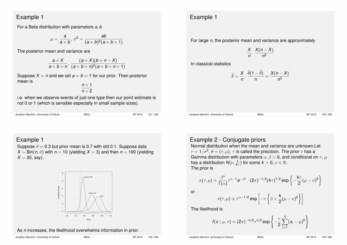
Example 1

For a Beta distribution with parameters a,b

µ =a

a + b, σ2 =

ab(a + b)2(a + b + 1)

The posterior mean and variance are

a + Xa + b + n

,(a + X )(b + n − X )

(a + b + n)2(a + b + n + 1)

Suppose X = n and we set a = b = 1 for our prior. Then posteriormean is

n + 1n + 2

i.e. when we observe events of just one type then our point estimate isnot 0 or 1 (which is sensible especially in small sample sizes).


Example 1

For large n, the posterior mean and variance are approximately

Xn,

X (n − X )

n3

In classical statistics

θ =Xn,θ(1− θ)

n=

X (n − X )

n3


Example 1Suppose ϑ = 0.3 but prior mean is 0.7 with std 0.1. Suppose dataX ∼ Bin(n, ϑ) with n = 10 (yielding X = 3) and then n = 100 (yieldingX = 30, say).

0.0 0.2 0.4 0.6 0.8 1.0

02

46

810

theta

prob

abilit

y de

nsity

priorpost n=10

post n=100

As n increases, the likelihood overwhelms information in prior.Jonathan Marchini (University of Oxford) BS2a MT 2013 103 / 282

Example 2 - Conjugate priorsNormal distribution when the mean and variance are unknown.Letτ = 1/σ2, θ = (τ, µ). τ is called the precision. The prior τ has aGamma distribution with parameters α, β > 0, and conditional on τ , µhas a distribution N(ν, 1

kτ ) for some k > 0, ν ∈ R.The prior is

π(τ, µ) =βα

Γ(α)τα−1e−βτ · (2π)−1/2(kτ)1/2 exp

{−kτ

2(µ− ν)2

}or

π(τ, µ) ∝ τα−1/2 exp[−τ{β +

k2

(µ− ν)2}]

The likelihood is

f (x | µ, τ) = (2π)−n/2τn/2 exp

{−τ

2

n∑i=1

(xi − µ)2

}


Example 2 - Conjugate priors

Thus

π(τ, µ | x) ∝ τα+(n/2)−1/2 exp

[−τ

{β +

k2

(µ− ν)2 +12

n∑i=1

(xi − µ)2

}]

Complete the square to see that

k(µ− ν)2 +∑

(xi − µ)2

= (k + n)

(µ− kν + nx

k + n

)2

+nk

n + k(x − ν)2 +

∑(xi − x)2


Example 2 - Conjugate priors

Thus the posterior is

π(τ, µ | x) ∝ τα′−1/2 exp[−τ{β′ +

k ′

2(ν ′ − µ)2

}]where

α′ = α +n2

β′ = β +12· nk

n + k(x − ν)2 +

12

∑(xi − x)2

k ′ = k + n

ν ′ =kν + nx

k + n

This is the same form as the prior, so the class is conjugate prior.


Lecture 7 : Prior distributions. Hierarchical models. PredictiveDistributions.


Constructing priors

Subjective Priors: Write down a distribution representing priorknowledge about the parameter before the data is available. Ifpossible, build a model for the parameter. If different scientists havedifferent priors or it is unclear how to represent prior knowledge as adistribution, then consider several different priors. Repeat the analysisand check that conclusions are insensitive to priors representing’different points of view’.Non-Subjective Priors: Several approaches offer the promise of an’automatic’ and even ’objective’ prior. We list some suggestions below(Uniform, Jeffreys, MaxEnt). In practice, if one of these priorsconflicted prior knowledge, we wouldnt use it. These approaches canbe useful to complete the specification of a prior distribution, oncesubjective considerations have been taken into account.


Uniform priorsIf we use a uniform prior (π(θ) ∝ constant) then

π(θ|x) = L(θ; x)/

∫Θ

L(θ; x)dθ

and∫

Θ L(θ; x)dθ may not be finite. Such distributions are calledimproper and all inference is meaningless.

Example X ∼ Exp(1/µ) and N = I(X < 1) yielding N = n withn ∈ {0,1}. Suppose we observe n = 0. Now

L(µ; n) = exp(−1/µ)

so if we take π(µ) ∝ 1 for µ > 0 we have

π(µ|n) ∝ exp(−1/µ)

which is improper, as π(µ|n)→ 1 as µ→∞ so∫∞

0 exp(−1/µ)dµcannot exist.


Jeffreys’ PriorsJeffreys reasoned as follows. If we have a rule for constructing priors itshould lead to the same distribution if we apply it to θ or some otherparameterization ψ with g(ψ) = θ.Jeffreys took

π(θ) ∝√

Iθ where Iθ = E

[(∂`

∂θ

)2]

is the Fisher information. Now if g(ψ) = θ then

πΨ(ψ) ∝ π(g(ψ))|g′(ψ)|,

so Jeffreys rule should yield πΨ(ψ) ∝√

Ig(ψ)|g′(ψ)|. The rule givesπΨ(ψ) ∝

√Iψ. But Iψ = g′(ψ)2Ig(ψ), so√

Iψ =√

Ig(ψ)|g′(ψ)|

and the rule is consistent in this respect.It is sometimes desirable (on subjective grounds) to have a prior whichis invariant under reparameterization.


Higher dimensions

If Θ ⊂ Rk , and `(θ; X ) = log(f (X ; θ)), the Fisher information

[Iθ]i,j = −Eθ(∂2`(θ; X )

∂θi∂θj

)satisfies

−Eθ(∂2`(θ; X )

∂θi∂θj

)= Eθ

(∂`(θ; X )

∂θi

∂`(θ; X )

∂θj

)subject to regularity conditions. A k -dimensional Jeffreys’ prior

π(θ) ∝ |Iθ|1/2

(|A| ≡ det(A)) is invariant under 1-1 reparameterization.Exercise Verify 1 to 1 g(ψ) = θ in Rk gives πΨ(ψ) =

√Ig(ψ)

∣∣∣∂θT

∂ψ

∣∣∣.Jonathan Marchini (University of Oxford) BS2a MT 2013 111 / 282

Maximum Entropy PriorsChoose a density π(θ) which maximizes the entropy

φ[π] = −∫

Θπ(θ) logπ(θ)dθ

over functions π(θ) subject to constraints on π. This is a Calculus ofVariations problem.Example The distribution π maximizing φ[π] over all densities π onΘ = R, subject to∫ ∞

0π(θ)dθ = 1,

∫ ∞0

θπ(θ)dθ = µ, and∫ ∞

0(θ − µ)2π(θ)dθ = σ2,

(normalized with Eϑ = µ and Var(ϑ) = σ2) is the normal density

π(θ) =1√

2πσ2e−(θ−µ)2/2σ2

.


This is a special case of the following Theorem.

Theorem The density π(θ) that maximizes φ(π), subject to

E[tj(θ)] = tj , j = 1, . . . ,p

takes the p-parameter exponential family form

π(θ) ∝ exp

{ p∑i=1

λi ti(θ)

}

for all θ ∈ Θ, where λ1, . . . , λp are determined by the constraints. (Forthe proof see Leonard and Hsu). Example In the normal caset1(θ) = θ, t1 = µ, t2(θ) = (θ − µ)2, t2 = σ2 givesπ(θ) ∝ exp(λ1θ + λ2(θ − µ)2). Impose the constraints to get λ1 = 0and λ2 = −1/2σ2.


ExampleSuppose prior probabilities are specified so that

P(aj−1 < ϑ ≤ aj) = φj , j = 1, . . . ,p

with∑

j φj = 1 and

ϑ ∈ (a0,ap), a0 ≤ a1 · · · ≤ ap ≤ ap.

We find the maximum entropy distribution subject to these conditions.The conditions are equivalent to

E[tj(ϑ)] = φj , j = 1, . . . ,p

where tj(ϑ) = I[aj−1 < ϑ ≤ aj ]. The posterior density of ϑ is

π(θ) ∝ exp

p∑

j=1

λjI[aj−1 < θ ≤ aj ]

, a0 ≤ θ ≤ ap

where λ1, . . . , λp are determined by the conditions. π(θ) is a histogram,with intervals (a0,a1], (a1,a2], . . . , (ap−1,ap].


Hierarchical modelsThese are models where the prior has parameters which again have aprobability distribution.

Data x have a density f (x ; θ).The prior distribution of θ is π(θ;ψ).ψ has a prior distribution g(ψ), for ψ ∈ Ψ.

We can work with posterior π(θ, ψ|x) ∝ f (x ; θ)π(θ;ψ)g(ψ), or

π(θ|x) =

∫Ψπ(θ, ψ|x)dψ ∝ f (x ; θ)

∫Ψπ(θ;ψ)g(ψ)dψ

∝ f (x ; θ)π(θ)

The hierarchical model simply specifies the prior for θ indirectly

π(θ) =

∫π(θ;ψ)g(ψ)dψ.


ExampleFor i = 1,2, ..., k we make ni observations Xi,1,Xi,2, ...,Xi,ni onpopulation i , with Xij ∼ N(θi , σ

2). The θi are the unknown means forobservations on the i ’th population but σ2 is known. Suppose the priormodel for the θi is iid normal, θi ∼ N(φ, τ2).

X1,1,…,X1,n1 ~ N θ1,σ

2( ) θ1

X2,1,…,X2,n2~ N θ2,σ

2( ) θ2

. . N φ,τ 2( ) . .

Xk,1,…,Xk,nk~ N θk,σ

2( ) θk!


Example

If ψ = (φ, τ2)

π(θ1, . . . , θk ;ψ) =k∏

i=1

(2πτ2)−1/2 exp{− 1

2τ2 (θi − φ)2},

Now we need a prior for φ and τ2. Suppose we take

g(φ, τ2) = constant,

so all possible φ, τ2 equally likely a priori. careful!.

The joint posterior of the parameters is

π(θ, ψ|x) ∝ f (x ; θ)π(θ|ψ)g(ψ)


ExampleIntegration with respect to ψ gives the posterior density of θ.

π(θ, φ, τ2|x) ∝

k∏i=1

exp

− 12σ2

ni∑j=1

(xij − θi)2

×

[k∏

i=1

τ−1 exp{− 1

2τ2 (θi − φ)2}]

Integrate out wrt φ and τ2 to obtain the marginal posterior distributionof θ. Exercise Integrating the last factor wrt φ gives a termproportional to

τ1−k exp{− 1

2τ2

∑(θi − θ)2

}Exercise Then the integral wrt τ gives a term proportional to[∑

(θi − θ)2]1−k/2


ExampleThus the posterior distribution of θ is

π(θ|x) ∝

k∏i=1

exp

− 12σ2

ni∑j=1

(xij − θi)2

· [∑(θi − θ)2

]1−k/2

∝

[k∏

i=1

exp{− 1

2σ2 ni(θi − xi)2}]·[∑

(θi − θ)2]1−k/2

where xi =∑

j xij/ni . Let θj be the MAP estimate for θj (posteriormode) and put θ∗ =

∑θj/k . Exercise Differentiate π(θ|x) wrt θj and

set to equal zero to get

θj = (ωj xj + νθ∗)/(ωj + ν),

where ωj = (σ2/nj)−1 and ν =

[∑(θi − θ∗)2/(k − 2)

]−1.

If the θj were unrelated then θj = xj . The model modifies the estimateby pulling it towards the mean of the estimated θis.


Uniform priors

If the prior is uniform (and possibly improper itself) but the posterior isproper, and it can be shown that all parameter values being equallyprobable a priori is a fair representation of prior knowledge, then theuniform prior may be useful.

In the hierarchical model in the previous example the prior on ϕ, τ2

was improper, but the posterior is proper.


Priors for Exponential Families

Conjugate prior for an exponential family

f (x | θ) = exp

k∑

j=1

Aj(θ)n∑

i=1

Bj(xi) +n∑

i=1

C(xi) + nD(θ)

The prior distribution based on sufficient statistics

π(θ) ∝ exp{τ0D(θ) +k∑

j=1

Aj(θ)τj}

(where (τ0, . . . , τk ) are constant prior parameters) is conjugate.


Priors for Exponential Families

The posterior density is proportional to

f (x | θ)π(θ | τ0, . . . , τk )

∝ exp

k∑

j=1

Aj(θ)

[n∑

i=1

Bj(xi) + τj

]+ (n + τ0)D(θ)

This is an updated form of the prior with

B′j (x) =n∑

i=1

Bj(xi) + τj

n′ = n + τ0


f


Predictive distributions

X1, . . . ,Xn are observations from f (x ; θ) and the predictive distributionof a further observation Xn+1 is required.

If x = (x1, . . . , xn) then the posterior predictive distribution is

g(xn+1 | x) =

∫f (xn+1; θ)π(θ | x)dθ

Predictive distributions are useful for ...prediction.

They are used also for model checking. Divide the data in two groups,Y = (X1, ...,Xa) and Z = (Xa+1, ...,Xn). If we fit using Y and check thatthe ‘reserved data’ Z overlap g(xn+1 | x) in distribution.


Example

Data X1, . . . ,Xn are iid N(θ, σ2) with σ2 known and prior θ ∼ N(µ0, σ20).

Predict Xn+1.

We saw that π(θ | x) = N(θ;µ1, σ21) with µ1 and σ1 calculated in

example 3 above.

In order to calculate the posterior predictive density for Xn+1 we needto evaluate

g(xn+1 | x) =

∫ ∞−∞

1√2πσ2

e−(x−θ)2

2σ21√

2πσ21

e− (θ−µ1)2

2σ21 dθ

We could complete the square to solve this.


Example

Alternatively, think how Xn+1 is built up.

We have θ|X ∼ N(µ1, σ21) and Xn+1|θ ∼ N(θ, σ2).

If Y ,Z ∼ N(0,1) then

θ = µ1 + σ1Z (posterior)Xn+1 = θ + σY (observation model)

= µ1 + σ1Z + σY .

It follows that Xn+1 ∼ N(µ1, σ2 + σ2

1) is the posterior predictive densityfor Xn+1|X1, ...,Xn.


Lecture 8 : Bayesian Hypothesis Testing


Hypothesis Testing I

In Bayesian inference, hypotheses are represented by priordistributions. There is nothing special about H0, and H0 and H1 neednot be nested.Let π(θ|H0), θ ∈ Θ0 be the prior distribution of θ under hypothesis H0.Here π(θ|H0) is a pmf/pfd as θ|H0 is continuous/discrete.Composite H0 : θ ∈ Θ0, with Θ0 ⊂ Θ,

π(θ|H0) =π(θ)

π(θ ∈ Θ0)I(θ ∈ Θ0)

If Θ0 has more than one element then H0 is a composite hypothesis.Simple H0 : θ = θ0, so that π(θ0|H0) = 1. This is a simple hypothesis.However, since any statement about the form of the prior amounts to ahypothesis about θ, we are not restricted to statements about setmembership (not just simple and composite).


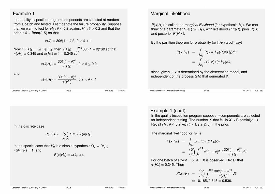
Example 1In a quality inspection program components are selected at randomfrom a batch and tested. Let θ denote the failure probability. Supposethat we want to test for H0 : θ ≤ 0.2 against H1 : θ > 0.2 and that theprior is θ ∼ Beta(2,5) so that

π(θ) = 30θ(1− θ)4, 0 < θ < 1.

Now if π(H0) = π(θ ∈ Θ0) then π(H0) =∫ 0.2

0 30θ(1− θ)4dθ so thatπ(H0) ' 0.345 and π(H0) ' 1− 0.345 so

π(θ|H0) =30θ(1− θ)4

π(H0), 0 < θ ≤ 0.2

and

π(θ|H1) =30θ(1− θ)4

π(H1), 0.2 < θ < 1


Marginal Likelihood

P(x |H0) is called the marginal likelihood (for hypothesis H0). We canthink of a parameter H ∈ {H0,H1}, with likelihood P(x |H), prior P(H)and posterior P(H|x).

By the partition theorem for probability (π(θ|H0) a pdf, say)

P(x |H0) =

∫Θ0

P(x |θ,H0)P(θ|H0)dθ

=

∫Θ0

L(θ; x)π(θ|H0)dθ,

since, given θ, x is determined by the observation model, andindependent of the process (H0) that generated θ.


In the discrete case

P(x |H0) =∑θ∈Θ0

L(θ; x)π(θ|H0).

In the special case that H0 is a simple hypothesis Θ0 = {θ0},π(θ0|H0) = 1, and

P(x |H0) = L(θ0; x).


Example 1 (cont)In the quality inspection program suppose n components are selectedfor independent testing. The number X that fail is X ∼ Binomial(n, θ).Recall H0 : θ ≤ 0.2 with θ ∼ Beta(2,5) in the prior.

The marginal likelihood for H0 is

P(x |H0) =

∫Θ0

L(θ; x)π(θ|H0)dθ

=

(5x

)∫ 0.2

0θx (1− θ)n−x 30θ(1− θ)4

π(H0)dθ

For one batch of size n = 5, X = 0 is observed. Recall thatπ(H0) ' 0.345. Then

P(x |H0) =

(50

)∫ 0.2

0

30θ(1− θ)9

π(H0)dθ

' 0.185/0.345 = 0.536.


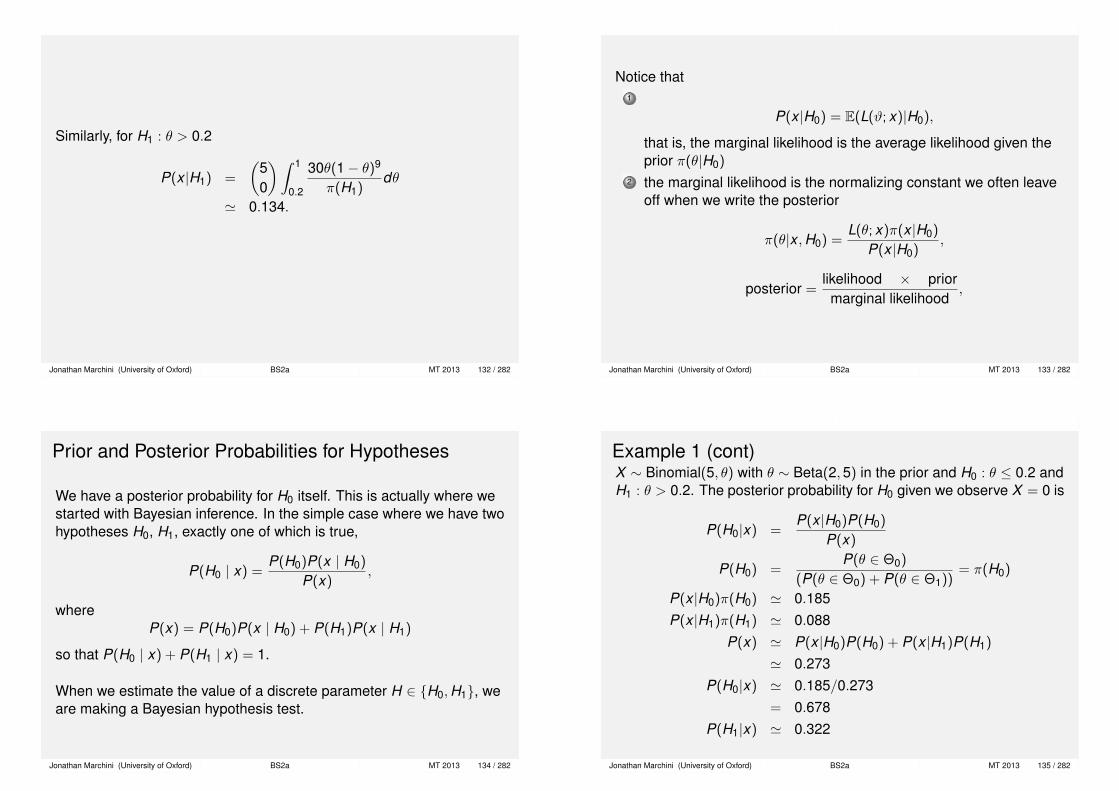
Similarly, for H1 : θ > 0.2

P(x |H1) =

(50

)∫ 1

0.2

30θ(1− θ)9

π(H1)dθ

' 0.134.


Notice that1

P(x |H0) = E(L(ϑ; x)|H0),

that is, the marginal likelihood is the average likelihood given theprior π(θ|H0)

2 the marginal likelihood is the normalizing constant we often leaveoff when we write the posterior

π(θ|x ,H0) =L(θ; x)π(x |H0)

P(x |H0),

posterior =likelihood × prior

marginal likelihood,


Prior and Posterior Probabilities for Hypotheses

We have a posterior probability for H0 itself. This is actually where westarted with Bayesian inference. In the simple case where we have twohypotheses H0, H1, exactly one of which is true,

P(H0 | x) =P(H0)P(x | H0)

P(x),

whereP(x) = P(H0)P(x | H0) + P(H1)P(x | H1)

so that P(H0 | x) + P(H1 | x) = 1.

When we estimate the value of a discrete parameter H ∈ {H0,H1}, weare making a Bayesian hypothesis test.


Example 1 (cont)X ∼ Binomial(5, θ) with θ ∼ Beta(2,5) in the prior and H0 : θ ≤ 0.2 andH1 : θ > 0.2. The posterior probability for H0 given we observe X = 0 is

P(H0|x) =P(x |H0)P(H0)

P(x)

P(H0) =P(θ ∈ Θ0)

(P(θ ∈ Θ0) + P(θ ∈ Θ1))= π(H0)

P(x |H0)π(H0) ' 0.185P(x |H1)π(H1) ' 0.088

P(x) ' P(x |H0)P(H0) + P(x |H1)P(H1)

' 0.273P(H0|x) ' 0.185/0.273

= 0.678P(H1|x) ' 0.322


Hypothesis Testing II, Bayes factors

Suppose we have two hypotheses H0, H1, exactly one of which is true.Data x .

The Prior OddsQ =

P[H0]

P[H1]

These are prior odds since P[H1] = 1− P[H0]. Here H0 is Q timesmore probable than H1, given the prior model.

The Posterior OddsQ∗ =

P[H0 | x ]

P[H1 | x ]

are the posterior odds, so that H0 is Q∗ times more probable than H1,given the data and prior model.


Hypothesis Testing II, Bayes factorsThe posterior odds for H0 against H1 can be written

Q∗ =P[H0]

P[H1]× P(x | H0)

P(x | H1)= Q × B

where Q is the prior odds and

B =P(x | H0)

P(x | H1)

is the Bayes Factor.

The Bayes Factor is a criterion for model comparison since H0 is Btimes more probable than H1, given the data and a prior model whichputs equal probability on H0 and H1. The Bayes factor tells us how thedata shifts the strength of belief (measured as a probability) in H0relative to H1.


Example 1 (cont)X ∼ Binomial(5, θ) with θ ∼ Beta(2,5) in the prior and H0 : θ ≤ 0.2 andH1 : θ > 0.2.

The prior odds are

Q = P(H0)/P(H1)

' 0.345/(1− 0.345) ' 0.527

The posterior odds are

Q∗ = P(H0|x)/P(H1|x)

' 0.678/(1− 0.678) ' 2.1

The Bayes factor comparing H0 and H1 is

B =P(x |H0)

P(x |H1)

' 0.536/0.134 = 4


Explicitly, from the beginning,

B =

∫Θ0

L(x ; θ)π(θ|H0)dθ∫Θ1

L(x ; θ)π(θ|H1)dθ

=

∫Θ0

L(x ; θ)π(θ)dθ∫Θ1

L(x ; θ)π(θ)dθ× π(H1)

π(H0)

=

(50

) ∫ 0.20 30θ(1− θ)9dθ(5

0

) ∫ 10.2 30θ(1− θ)9dθ

∫ 10.2 30θ(1− θ)4dθ∫ 0.20 30θ(1− θ)4dθ

= 6619897/1654272 ' 4.002 (Maple).

This is ’positive’ evidence for θ ≤ 0.2. Notice that the Bayes factor is’more positive’ than the posterior odds, as the prior odds wereweighted against H0.


Interpreting Bayes Factors

Adrian Raftery gives this table (values are approximate, and adaptedfrom a table due to Jeffreys) interpreting B.

‘P(H0|x)’ B 2 log(B) evidence for H0< 0.5 < 1 < 0 negative (supports H1)0.5 to 0.75 1 to 3 0 to 2 barely worth mentioning0.75 to 0.92 3 to 12 2 to 5 positive0.92 to 0.99 12 to 150 5 to 10 strong> 0.99 > 150 > 10 very strong

I added the leftmost column (posterior for prior odds equal one). Wesometimes report 2 log(B) because it is on the same scale as thefamiliar deviance and likelihood ratio test statistic.


Simple-Simple hypothesis

If both hypotheses are simple H0 : θ = θ0; H1 : θ = θ1, with priorsP(H0) and P(H1) for the two hypotheses, the posterior probability forH0 is

P(H0|x) =P(x |H0)P(H0)

P(x)

=L(θ0; x)P(H0)

L(θ0; x)P(H0) + L(θ1; x)P(H1),

since P(x |H0) is just L(θ0; x). The Bayes factor is then just likelihoodratio

B =L(θ0; x)

L(θ1; x).


Simple-Composite hypothesis

If one hypothesis is simple and the other composite, for example,H0 : θ = θ0; H1 : π(θ|H1), θ ∈ Θ, with priors P(H0) and P(H1) for thetwo hypotheses, the Bayes factor is

B =L(x ; θ0)∫

Θ L(x ; θ)π(θ|H1)dθ

The denominator is just∫

Θ L(x ; θ)π(θ)dθ when π(θ|H1) is a pdf.

Exercise Show that the posterior probability for H0 is

P(H0|x) =L(θ0; x)P(H0)

P(H0)L(θ0; x) + P(H1)∫

Θ L(x ; θ)π(θ)dθ

when π(θ|H1) is a pdf, in this simple-composite comparison.


ExampleX1, . . . ,Xn are iid N(θ, σ2), with σ2 known.H0 : θ = 0, H1 : θ|H1 ∼ N(µ, τ2). Bayes factor is P0/P1, where

P0 = (2πσ2)−n/2 exp(− 1

2σ2

∑x2

i

)P1 = (2πσ2)−n/2

∫ ∞−∞

exp(− 1

2σ2

∑(xi − θ)2

)×(2πτ2)−1/2 exp

(−(θ − µ)2

2τ2

)dθ.

Completing the square in P1 and integrating dθ,

P1 = (2πσ2)−n/2(

σ2

nτ2 + σ2

)1/2

×exp[−1

2

{n

nτ2 + σ2 (x − µ)2 +1σ2

∑(xi − x)2

}]Jonathan Marchini (University of Oxford) BS2a MT 2013 143 / 282

So

B =

(1 +

nτ2

σ2

)1/2

exp[−1

2

{nx2

σ2 −n

nτ2 + σ2 (x − µ)2}]

Defining t =√

nx/σ, η = −µ/τ, ρ = σ/(τ√

n), this can be written as

B =

(1 +

1ρ2

)1/2

exp[−1

2

{(t − ρη)2

1 + ρ2 − η2}]

This example illustrates a problem choosing the prior. If we take adiffuse prior, for ρ so that ρ→ 0, then B →∞, giving overwelmingsupport for H0.This is an instance of Lindley’s paradox. The point here is that Bcompares the models θ = θ0 and θ ∼ π(·|H1), not the sets θ0 againstθ \ {θ0}. If the π(θ|H1)-prior becomes very diffuse then the averagelikelihood (ie P(H1|x), the marginal likelihood, which is thedenominator of B) goes to zero, while P(H0|x) = L(θ0; x) is fixed.


Lecture 9 : Decision theory


Decision theory

Example You have been exposed to a deadly virus. About 1/3 ofpeople who are exposed to the virus are infected by it, and all thoseinfected by it die unless they receive a vaccine. By the time anysymptoms of the virus show up, it is too late for the vaccine to work.You are offered a vaccine for £500. Do you take it or not?

The most likely scenario is that you don’t have the virus but basing adecision on this ignores the costs (or loss) associated with thedecisions. We would put a very high loss on dying!


Decision Theory

Decision Theory sits ‘above’ Bayesian and classical statisticalinference and gives us a basis to compare different approaches tostatistical inference.We make decisions by applying rules to data.Decisions are subject to risk.A risk function specifies the expected loss which follows from theapplication of a given rule, and this is a basis for comparing rules.We may choose a rule to minimize the maximum risk, or we maychoose a rule to minimize the average risk.


Terminology

θ is the ‘true state of nature’, X ∼ f (x ; θ) is the data.

The Decision rule is δ. If X = x , adopt the action δ(x) given by therule.

Example A single parameter θ is estimated from X = x by δ(x) = θ(x).

The rule θ is the functional form of the estimator. The action is thevalue of the estimator.

The Loss function LS(θ, δ(x)) measures the loss from action δ(x)when θ holds.


ExampleLS(θ, θ(x)) is the loss function which increases for θ(x) being awayfrom θ. Here are three common loss functions.Zero-One loss

LS(θ, θ(x)) =

{0 |θ(x)− θ| < ba |θ(x)− θ| ≥ b

where a,b are constants.

Absolute error loss

LS(θ, θ(x)) = a|θ(x)− θ|

where a > 0.

Quadratic lossLS(θ, θ(x)) = (θ(x)− θ)2.


Example

θ b -‐b

a

θ

θ

Zero-‐One Loss

Absolute error loss

Quadra3c loss


Risk function

Definition The risk function R(θ, δ) is defined as

R(θ, δ) =

∫LS(θ, δ(x))f (x ; θ)dx ,

This is the expected value of the loss (aka expected loss).

Example In the context of point estimation, with Quadratic Loss, therisk function is the mean square error,

R(θ, θ) = E[(θ(X )− θ)2].


Admissible and inadmissible rules.

Definition A procedure δ1 is inadmissible if there exists anotherprocedure δ2 such that

R(θ, δ1) ≥ R(θ, δ2), for all θ ∈ Θ

with R(θ, δ1) > R(θ, δ2) for at least some θ.

A procedure which is not inadmissible is admissible.


ExampleSuppose X ∼ U(0, θ). Consider estimators of the form θ(x) = ax (thisis a family of decisions rules indexed by a).

Show that a = 3/2 is a necessary condition for the rule θ to beadmissible for quadratic loss.

R(θ, θ) =

∫ θ

0(ax − θ)2 1

θdx

= (a2/3− a + 1)θ2

and R is minimized at a = 3/2.

This does not show θ(x) = 3x/2 is admissible here.

It only shows that all estimators with a 6= 3/2 are inadmissible. Theestimator θ(x) = 3x/2 maybe inadmissible relative to other estimatorsnot in this class.


Minimax rules

Definition A rule δ is a minimax rule if maxθ R(θ, δ) ≤ maxθ R(θ, δ′) forany other rule δ′. It minimizes the maximum risk.

Since minimax minimizes the maximum risk (ie, the loss averaged overall possible data X ∼ f ) the choice of rule is not influenced by theactual data X = x (though given the rule δ, the action δ(x) isdata-dependent).

It makes sense when the maximum loss scenario must be avoided, butcan can lead to poor performance on average.


Bayes risk, Bayes rule, expected posterior lossDefinition Suppose we have a prior probability π = π(θ) for θ. Denoteby

r(π, δ) =

∫R(θ, δ)π(θ)dθ

the Bayes risk of rule δ. A Bayes rule is a rule that minimizes theBayes risk. A Bayes rule is sometimes called a Bayes procedure.

Let π(θ|x) =L(x ; θ)π(θ)

h(x)denote the posterior following from likelihood

L and prior π.

Definition The expected posterior loss is defined as∫LS(θ, δ(x))π(θ|x)dθ


Lemma A Bayes rule minimizes the expected posterior loss.

Proof ∫R(θ, δ)π(θ)dθ =

∫ ∫LS(θ, δ(x))L(θ; x)π(θ)dx dθ

=

∫ ∫LS(θ, δ(x))π(θ|x)h(x)dx dθ

=

∫h(x)

(∫LS(θ, δ(x))π(θ|x)dθ

)dx

That is for each x we choose δ(x) to minimize the integral∫LS(θ, δ(x))π(θ|x)dθ


Bayes rules for Point estimationZero-One loss

LS(θ, θ(x)) =

{0 |θ(x)− θ| < ba |θ(x)− θ| ≥ b

where a,b are constants.

We need to minimize∫ ∞−∞

π(θ|x)LS(θ, θ)dθ = a∫ ∞θ+b

π(θ|x)dθ + a∫ θ−b

−∞π(θ|x)dθ

∝ 1−∫ θ+b

θ−bπ(θ|x)dθ

That is we want to maximize∫ θ+b

θ−bπ(θ|x)dθ


Zero-one lossIf π(θ|x) is unimodal the maximum is attained by choosing θ to be themid-point of the interval of length 2b for which π(θ|b) has the samevalue at both ends.

θ

As b → 0, θ → the global mode of the posterior distribution. If π(θ|x) isunimodal and symmetric, the optimal θ is the median (equal to themean and mode) of the posterior distribution.


Absolute error loss

Absolute error loss

LS(θ, θ(x)) = a|θ(x)− θ|

We need to minimise∫|θ − θ|π(θ|x)dθ =

∫ θ

−∞(θ − θ)π(θ|x)dθ +

∫ ∞θ

(θ − θ)π(θ|x)dθ.

Differentiate wrt θ and equate to zero.∫ θ

−∞π(θ|x)dθ −

∫ ∞θ

π(θ|x)dθ = 0

That is, the optimal θ is the median of the posterior distribution.


Quadratic loss

Minimize

Eθ|x [(θ − θ)2] = Eθ|x [(θ − θ + θ − θ)2]

= (θ − θ)2 + 2(θ − θ)Eθ|x (θ − θ) + Eθ|x [(θ − θ)2]

where θ is the posterior mean of θ.

Note θ and θ are constants in the posterior distribution of θ so that(θ − θ)E(θ − θ) = 0. So

Eθ|x [(θ − θ)2] = (θ − θ)2 + Vθ|x (θ)

The Quadratic loss function is minimized when θ = θ, the posteriormean.


Summary

The form of the Bayes rule depends upon the loss function in thefollowing way

Zero-one loss (as b → 0) leads to the posterior mode.Absolute error loss leads to the posterior median.Quadratic loss leads to the posterior mean.

Note These are not the only loss functions one could use in a givensituation, and other loss functions will lead to different Bayes rules.


ExampleX ∼ Binomial (n, θ), and the prior π(θ) is a Beta (α, β) distribution.

E(θ) =α

α + β

The distribution is unimodal if α, β > 1 with mode (α− 1)/(α + β − 2).

The posterior distribution of θ | x is Beta (α + x , β + n − x).

With zero-one loss and b → 0 the Bayes estimator is(α + x − 1)/(α + β + n − 2).

For a quadratic loss function, the Bayes estimator is(α + x)/(α + β + n).

For an absolute error loss function is the median of the posterior.


Lecture 10 : Finding minimax rules. Hypothesis testing with lossfunctions.


Minimax rulesDefinition A rule δ is a minimax rule if maxθ R(θ, δ) ≤ maxθ R(θ, δ′) forany other rule δ′. It minimizes the maximum risk.

Sometimes this doesn’t produce a sensible choice of decision rule.

0.0 0.2 0.4 0.6 0.8 1.0

0.0

0.5

1.0

1.5

e

Ris

k fu

nctio

n

d1

d2

−3 −2 −1 0 1 2 3

0.0

0.1

0.2

0.3

0.4

0.5

e

Ris

k fu

nctio

nd1

d2


Finding minimax rulesTheorem 1 If δ is a Bayes rule for prior π, with r(π, δ) = C, and δ0 is arule for which maxθ R(θ, δ0) = C, then δ0 is minimax.

Proof If for some other rule δ′, maxθ R(θ, δ′) = C − ε for some ε > 0(so δ0 is not minimax), then

r(π, δ′) =

∫R(θ, δ′)π(θ)dθ

≤∫

(C − ε)π(θ)dθ

= (C − ε)< r(π, δ)

so δ is not the Bayes rule for π, a contradiction. [This is an informaltreatment which assumes the min and max exist - see Y&S Ch 2 Sec2.6]


Finding minimax rules

Theorem 2 If δ is a Bayes rule for prior π with the property that R(θ, δ)does not depend on θ, then δ is minimax.

Proof (Y&S Ch 2) Let R(θ, δ) = C (no θ dependence). This implies

r(π, δ) =

∫R(θ, δ)π(θ)dθ = C.

If for some other rule δ′, maxθ R(θ, δ′) = C − ε for some ε > 0 (so δ0 isnot minimax), then we have r(π, δ′) ≤ C − ε. But r(π, δ) = C so δ is notthe Bayes rule for π, a contradiction.


Finding minimax rules

Theorem 2 tells us that

The Bayes estimator with constant risk is minimax.

This result is useful, as it gives an approach to finding minimax rules.

Bayes rules are sometimes easy to compute, so if we find a prior thatyields a Bayes rule with constant risk for all θ we have the minimaxrule.


Example : minimax estimator for quadratic lossX is Binomial (n, θ), and the prior π(θ) is a Beta (α, β) distribution. Fora quadratic loss function, the Bayes estimator is (α + X )/(α + β + n)

The risk function is

EX |θ[(θ − θ)2] = MSE(θ) = [Bias(θ)]2 + Var[θ]

=

[θ − E

(α + X

α + β + n

)]2

+ Var[

α + Xα + β + n

]=

[θ −

(α + nθ

α + β + n

)]2

+nθ(1− θ)

(α + β + n)2

=[θ(α + β)− α]2 + nθ(1− θ)

[α + β + n]2

The Bayes estimator with constant risk is minimax. This occurs whenα = β =

√n/2, so the minimax estimator using quadratic loss is

(α + x)/(α + β + n) = (x +√

n/2)/(n +√

n).Jonathan Marchini (University of Oxford) BS2a MT 2013 168 / 282

Hypothesis testing with loss functions

Suppose Xi ∼ f (x ; θ) iid for i = 1,2, ...,n and we wish to testH0 : θ = θ0 against H1 : θ = θ1.

The decision rule is δC when we use a critical region C so δC(x) = H1if x ∈ C and otherwise δC(x) = H0.

Loss function:

LS(θ, δC(x)) =

a θ = θ0, x ∈ C0 θ = θ0, x 6∈ Cb θ = θ1, x 6∈ C0 θ = θ1, x ∈ C

so the loss for Type I error is a (H0 holds and we accept H1) and theloss for Type II error is b (H1 holds and we accept H0).


Hypothesis testing with loss functionsThe risk function for the rule δC is

R(θ0; δC) =

∫LS(θ0, δC(x))f (x ; θ0)dx

=

∫aI(x ∈ C)f (x ; θ0)dx

= aα

as α = P(X ∈ C|H0) is the probability for Type I error.

SimilarlyR(θ1; δC) = bβ,

as β = P(X 6∈ C|H1) is the probability for a Type II error.

Note α and β are functions of the critical region C.


Hypothesis testing with loss functions

To calculate the Bayes risk we need a prior. Let π(θ0) = p0 andπ(θ1) = p1 be the prior probabilities that H0 and H1 hold.

The Bayes risk is

r(π, δC) =∑

θ∈{θ0,θ1}

R(θ; δC)π(θ)

= p0aα(C) + p1bβ(C).

The Bayes test chooses the critical region C to minimize the Bayesrisk.

Question How do we do this?


Hypothesis testing with loss functionsTo answer this question, let’s revise what we know about Frequentisthypothesis testing.

Neyman-Pearson lemma The best test of size α of H0 vs H1 is alikelihood ratio test with critical region

C′ =

{x ;

L(θ1; x)

L(θ0; x)≥ A

}for some constant A > 0 chosen so that P(X ∈ C′|H0) = α.

By ‘best test’ we mean the test with the highest power, where Power =1 - Type II error.

In frequentist statistics we fix the Type I error (α) and this determinesthe value of A, thus defining the critical region for the test.


Bayes tests

The following theorem tells us how to choose the critical region tominimize the Bayes risk, in the same way that the Neyman-Pearsonlemma tells us how to maximize the power at fixed size.

Theorem The critical region for the Bayes test is the critical region fora LR test with

A =p0ap1b

Every LR test is a Bayes test for some p0,p1.


Proof

The Bayes test minimizes

p0aα + p1bβ = p0aP(X ∈ C|H0) + p1bP(X ∈ C′|H1)

= p0a∫

CL(θ0; x)dx + p1b

∫C′

L(θ1; x)dx

= p0a∫

CL(θ0; x)dx + p1b

[1−

∫C

L(θ1; x)dx]

= p1b +

∫C

[p0aL(θ0; x)− p1bL(θ1; x)

]dx

So choose C such that x ∈ C iff p0aL(θ0; x)− p1bL(θ1; x) ≤ 0, i.e.when

L(θ1; x)

L(θ0; x)≥ p0a

p1b


Example

Let X1, . . . ,Xn be N(µ, σ2) with σ2 known, and we want to testH0 : µ = µ0 vs H1 : µ = µ1, with µ1 > µ0. The critical region for the LRtest

L(θ1; x)

L(θ0; x)≥ A

becomes

x ≥ σ2 log(A)

n(µ1 − µ0)+

12

(µ0 + µ1) = B( say)

In the classical case we ignore the exact value of B, but in a Bayes testA = p0a/(p1b) and we substitute into B. As an example take

µ0 = 0, µ1 = 1, σ2 = 1,n = 4,a = 2,b = 1,p0 = 1/4,p1 = 3/4


Then the Bayes test has critical region

x ≥ 14

log(13× 2

1) +

12

=14

log(23

) +12

= 0.399

For this test (using the fact that X is N(µ,1/4))

α = P(X ≥ 0.3999 | µ = 0, σ2/n = 1/4) = 0.212

andβ = P(X < 0.3999 | µ = 1, σ2/n = 1/4) = 0.115

In a classical approach fixing α = 0.05, B = 1.645√

1/4 = 0.822, so

β = P(X < 0.822 | µ = 1, σ2 = 1/4) = 0.363

In the Bayes test α has been increased and β decreased.


Lecture 11 : Stein’s paradox and the James-Stein estimator. EmpiricalBayes


Stein’s paradox and the James-Stein EstimatorStein’s paradox has been described (Efron, 1992) as ‘the most strikingtheorem of post-war mathematical statistics’!

Theorem Let Xi ∼ N(µi ,1), i = 1,2, ...,p be jointly independent so wehave one data point for each of the p µi -parameters.

Let X = (X1, ...,Xp) and µ = (µ1, ..., µp). The MLE µ for µ is µMLE = X .This estimator is inadmissable for quadratic loss i.e. Risk = MSE.

The result is surprising since the estimator X is the MLE and alsoMVUE.

An estimator with lower risk is given by the James-Stein estimator

µJSE =

(1− a∑

i X 2i

)X


Implications of Stein’s Paradox

Suppose we are interested in estimating1 the weight of a randomly chosen loaf of bread from a supermarket.2 the height of a random chosen blade of grass from a garden.3 the speed of a randomly chosen car as it passes a speed camera.

These are totally unrelated quantities. It seem implausible that bycombining information across the data points that we might end upwith a better way of estimating the vector of three parameters.

The James-Stein estimator tells us that we can get a better estimate(on average) for the vector of three parameters by simultaneouslyusing the three unrelated measurements.


ProofConsider the alternative estimator

µJSE =

(1− a∑

i X 2i

)X (the James-Stein estimator)

Note This estimator ‘shrinks’ X towards 0 (when∑

i X 2i > a).

We will show that if a = p − 2 then R(µ, µJSE ) < R(µ, µMLE ) for everyµ ∈ Rn, so that the MLE is inadmissable in this case.

First, the risk for µMLE is

R(µ, µMLE ) =

p∑i=1

E(|µi − µMLE ,i |2) =

p∑i=1

E(|µi − Xi |2) = p

recognizing Var(Xi) = 1.Jonathan Marchini (University of Oxford) BS2a MT 2013 180 / 282

Stein’s LemmaIn order to calculate R(µ, µJSE ), it is convenient to use Stein’s Lemma,for Normal RV,

E((Xi − µ)h(X )) = E(∂h(X )

∂Xi

).

This can be shown by integrating by parts. Noting∫(xi − µ)e−(xi−µi )

2/2dx = −e−(xi−µi )2/2

we have∫ ∞−∞

(xi − µi)h(x)e−(xi−µi )2/2dxi = −h(x)e−(xi−µi )

2/2∣∣∣xi =∞

xi =−∞

+

∫ ∞−∞

∂h(x)

∂xie−(xi−µi )

2/2dxi

The first term is zero if h(x) (for eg) is bounded, giving the lemma.Jonathan Marchini (University of Oxford) BS2a MT 2013 181 / 282

Proof (continued)

R(µ, µJSE ) =

p∑i=1

E(|µi − µi |2) with µi =

(1− a∑

i X 2i

)Xi

E(|µi − µi |2) = E(|µi − Xi |2)− 2aE

((Xi − µi)Xi∑

j X 2j

)

+a2E

(X 2

i

(∑

j X 2j )2

)

E

((Xi − µi)Xi∑

j X 2j

)= E

(∂

∂Xi

Xi∑j X 2

j

)Stein’s lemma

= E

(∑j X 2

j − 2X 2i

(∑

j X 2j )2

)= E

(1∑j X 2

j− 2

X 2i

(∑

j X 2j )2

)


Putting the pieces together,

p∑i=1

E(|µi − µi |2) = R(µ, µMLE )− (2ap − 4a)E

(1∑j X 2

j

)+ a2E

(1∑j X 2

j

)

= p − (2a(p − 2)− a2)E

(1∑j X 2

j

)

and this is less than p if 2ap − 4a− a2 > 0 and in particular ata = p − 2, which minimizes the risk over a ∈ R.

Note We have not shown that the James Stein estimator is admissible.

Further reading Young and Smith sec 3.4 which covers theJames-Stein estimator is worth reading. It includes a nice example(sec 3.4.1) on the application of the estimator to estimation of baseballhome run rates.


The risk of the James-Stein estimatorRemember R(µ, µMLE ) = p. When a = p − 2

If µi = 0⇒ Xi ∼ N(0,1)⇒∑

j X 2j ∼ χ2

p ⇒ E(

1∑j X 2

j

)= 1/(p − 2)

⇒ R(µ, µJSE ) = 2.

If µi = λ⇒ Xi = λ+ Zi where Zi ∼ N(0,1) and∑

j X 2j ∼ λ2 + χ2

p

⇒ E(

1∑j X 2

j

)→ 0 as λ→∞ so R(µ, µJSE )→ p.

So we get a smaller difference between R(µ, µMLE ) and R(µ, µJSE ) as

E(

1∑j X 2

j

)gets smaller.

Exercise A better estimator is X1p +(

1− aV

)(X − X1p) where

V =∑p

j−1(Xj − X )2 and 1p is p-dimensional vector of 1’s.


Empirical Bayes

Bayes estimators have good risk properties (for example, the posteriormean is usually admissible for quadratic loss).

However, Bayes estimators may be hard to compute (for example, theposterior mean is an integral, or sum), particularly for hierarchicalmodels.

In Empirical Bayes, we use Bayesian reasoning to find estimatorswhich can then be used in classical frequentist. EB uses a particularstrategy to simplify hierarchical models.


Empirical BayesRecall the setup for Bayesian inference for hierarchical models.

X ∼ f (x ; θ)

θ ∼ π(θ;ψ)

ψ ∼ g(ψ)

Our prior for θ has a parameter ψ which also has a prior. The posterioris

π(θ, ψ|x) ∝ L(θ; x)π(θ;ψ)g(ψ)

If we want minimim risk for quadratic loss (for eg) we should use

θ =

∫ ∫θπ(θ, ψ|x)dθdψ


Empirical BayesThe EB trick is to avoid doing ψ-integrals by replacing ψ with anestimate ψ, derived from the data, and consider the model

X ∼ f (x ; θ)

θ ∼ π(θ; ψ)

This EB approximation to the full posterior ’chops off’ a layer of thehierarchy. The reduced model has posterior

π(θ|x) ∝ L(θ; x)π(θ; ψ),

and a Bayes estimator θEB is calculated using π(θ|x). For example, forquadratic loss,

θ =

∫θπ(θ|x)dθ.


Empirical Bayes

We still need an estimator for ψ. There are several choices.

We can use the MLE ψ = arg maxψ p(x |ψ) for ψ in the marginallikelihood

p(x |ψ) =

∫L(θ; x)π(θ;ψ)dθ.

Method of moments estimators are used also.


Example

The James-Stein estimator is an EB-estimator

Data xi ∼ N(θi ,1), i = 1, . . . ,p (so one observation xi for eachparameter θi ). The MLE for θi is simply θMLE ,i = xi . Construct an EBestimator for quadratic loss.

Suppose the prior is θi ∼ N(0, τ2) (we have some freedom here, as weare mainly interested in the risk-related properties of the finalestimator).

If we knew τ we have (completing the square - see Lecture 7 p13)

θi |(xi , τ) ∼ N(

xiτ2

1 + τ2 ,τ2

1 + τ2

).


ExampleTo get an estimate for τ we compute the marginal distribution for Xigiven τ , which is Xi ∼ N(0, τ2 + 1). The MLE for τ is thenτ2 = 1

p∑

i X 2i − 1, and this gives

θEB,i =Xi τ

2

1 + τ2

=

(1− p∑

i X 2i

)Xi

which is the James-Stein estimator

θJS,i =

(1− a∑

i X 2i

)Xi

with a = p. This isn’t the minimum risk JS estimator for quadratic loss,(that is a = p − 2) but it already beats the MLE for all θ. (to get the bestJS estimator (with a = p − 2) use a method of moments estimator forτ . See Young and Smith Section 3.5)


Example

Data xi ∼ Poisson(θi), i = 1, . . . ,n (so one observation xi for eachparameter θi ). The MLE for θi is simply θMLE ,i = xi . Construct an EBestimator for quadratic loss.

Suppose the prior for θi ’s is iid Exponential(λ) i.e. π(θi |λ) = λe−λθi .

p(xi | λ) =

∫ ∞0

e−θiθxii

xi !λe−λθi dθi

=

(1

1 + λ

)xi λ

1 + λ

⇒ given λ the x ′i s are iid geometric (λ/(1 + λ)).

The MLE of λ based on x1, . . . , xn is λ = 1/x , where x = 1n∑n

1 xi .


Now, under the EB simplification, set λ = λ, so that

π(θ|x) ∝ L(θ; x)π(θ|λ) =∏

i

e−θiθxii λe−λθi

and we recognise θi |x ∼ Γ(xi + 1, λ+ 1) in this EB approximation. Thisleads to an estimator

θEB,i =

∫θi π(θi |x)dθi

=xi + 1λ+ 1

= xxi + 1x + 1

We can rewrite this

θEB,i = xi +x

x + 1(x − xi)

showing that this EB estimator shrinks the estimates towards thecommon mean.


Lecture 12 : Markov Chain Monte Carlo. The Metropolis algorithm.


Computationally intensive methodsIn Bayesian inference, the things we need to know are often given interms of intractable integrals or sums.

If x ∼ f (x ; θ) and we have a prior π(θ) on θ ∈ Θ and we want tomeasure the evidence for θ ∈ S, S ⊂ Θ then we might calculate

P(θ ∈ S|x) =

∫Sπ(θ|x)dθ

where π(θ|x) ∝ f (x ; θ)π(θ) is the posterior density.

The posterior mean is commonly the most useful point estimate. Therewe have to compute

Eθ|xθ =

∫Θθπ(θ|x)dθ.

In previous examples our choice of prior has kept calculations doable.Jonathan Marchini (University of Oxford) BS2a MT 2013 194 / 282

Monte Carlo estimationP(θ ∈ S|x) = Eθ|xI(θ ∈ S) and Eθ|xθ are both averages.

If we have N iid samples θ(i) ∼ π(θ|x), i = 1,2, ...,N distributedaccording to the posterior density and we want to estimate a finitemean µf = Eθ|x f (θ) for some given function f , and we take

fN =1N

∑i

f (θ(i))

thenfN

P→ µf ,

that is, fN is consistent for estimation of µf (in fact there is usually aCLT).

But how do we generate the samples θ(i) ∼ π(θ|x), i = 1,2, ...,N?


Markov Chain Monte Carlo estimationThe idea in MCMC is to simulate an ergodic Markov Chainθ(i) i = 1,2, ...,N that has π(θ|x) as its stationary distribution.

Remember a discrete time Markov chain is specified by it’s transitionfunction

P(θ, θ′) = P(θ(t+1) = θ′|θ(t) = θ)

Given θ(0) we use the transition function to draw θ(1), then θ(2) givenθ(1), then θ(3) given θ(2) etc.

So we obtain a sequence θ(0), θ(1), θ(2), θ(3), θ(4), θ(5), θ(6), θ(7), . . .

The sequence of simulated θ-values θ(i) i = 1,2, ...,N is correlated.

Note In what follows we will refer to π(θ|x) as the target, and we willdrop the “|x” while we are setting up the theory.


Markov Chain Monte Carlo estimationHowever, the ergodic theorem for Markov chains from Part A tells usthat

1N

∑i

f (θ(i))P→ µf

so we can use the Markov Chain sequence to form estimates.

The key here is that we can often write down an ergodic Markov chainthat is easy to simulate, and has stationary distribution π(θ|x).

Question If we start from π(θ|x) how do we choose the transitionfunction P(θ, θ′)?

We will learn about two methods to do this1 The Metropolis algorithm2 Gibbs sampling


Metropolis algorithmFor target π(θ|x).

Suppose θ(t) = θ. Simulate a value for θ(t+1) as follows.1 Simulate a candidate state θ′ ∼ q(θ′|θ) i.e. a simple random

change to the state satisfying

q(θ′|θ) = q(θ|θ′)

2 With probability α(θ′|θ), set θ(t+1) = θ′ (accept) and otherwise setθ(t+1) = θ (reject). Here

α(θ′|θ) = min{

1,π(θ′|x)

π(θ|x)

}The overall transition probability from θ to θ′ is

P(θ, θ′) = q(θ′|θ)α(θ′|θ)


Example

In a population of m individuals N are red and m − N are blue, withunknown true value N unknown. A sample of k individuals is taken,with replacement, and X are red. The prior on N is uniform 0 to m.The posterior for N = n is

π(n | x) ∝ nx (m − n)k−x , n ∈ {0,1,2, ...,m}

In this example we can work out posterior probabilities exactly. Let ususe MCMC to estimate posterior probabilities, and check it matchesthe exact result (within Monte Carlo error).

We need to write an MCMC algorithm simulating a Markov chainN(t), t = 0,1,2, ... with the property that N(t) ∼ π(n | x).


ExampleMetropolis algorithm targeting π(n|x). See R code.

Suppose N(t) = n. Simulate a value for N(t+1) as follows.1 Toss a coin and set n′ = n + 1 on a Head and otherwise

n′ = n − 1. So q(n + 1|n) = q(n|n + 1) = 1/2.2 With probability

α(n′|n) = min{

1,π(n′|x)

π(n|x)

}set N(t+1) = n′ and otherwise set N(t+1) = n (reject).

Note that α = 0 if n′ = −1,m + 1 (since π(n′|x) = 0 in those cases)and otherwise

α(n′|n) = min{

1,(n′)x (m − n′)k−x

nx (m − n)k−x

}.


ExampleHere is a plot of showing the results of running the Markov chains for10,000 iterations. (m = 20, x = 3, k = 10)

0 2000 4000 6000 8000 10000

05

1015

20

t

N


ExampleHere is a plot showing the empirical density of the 10,000 samples,together with the true density in red. You can see that approximation isgood.

Histogram of N

N

Density

0 5 10 15 20

0.00

0.05

0.10

0.15


Why does it work?Theorem If θ(t), t = 0,1,2, ... is an irreducible, aperiodic Markov chainon a finite space Θ, satisfying detailed balance with respect to a targetdistribution π(θ) on Θ, and f : Θ→ R is a function with finite mean andvariance in π, then

1N

∑i

f (θ(i))P→ Eπf (θ)

[This is essentially a watered down version of the Ergodic Theorem ofPart A, with positive recurrence replaced by detailed balance]

Suppose Θ is finite. Let

P(n)(θ, θ′) = P(θ(t+n) = θ′|θ(t) = θ)

give the n-step transition probability in a homogeneous Markov chainwith transition probability P(θ, θ′).


Markov ChainsIrreducible

∀θ, θ′ ∈ Θ,∃n such that P(n)(θ, θ′) > 0,

Aperiodic∀θ ∈ Θ,gcd{n : P(n)(θ, θ) > 0} = 1

Detailed balance

π(θ)P(θ, θ′) = π(θ′)P(θ′, θ)

If detailed balance is satisfied the it is easy to show that the chain is astationary distribution ∑

θ∈Θ

π(θ)P(θ, θ′) = π(θ′).


Metropolis algorithmLet us check DB. Assume WLOG π(θ) ≥ π(θ′).

P(θ, θ′)π(θ) = q(θ′|θ)α(θ′|θ)π(θ) = q(θ′|θ) min{

1,π(θ′)

π(θ)

}π(θ)

= q(θ′|θ)π(θ′)

= q(θ|θ′) min{

1,π(θ)

π(θ′)

}π(θ′)

= P(θ′, θ)π(θ′),

since min{

1,π(θ′)

π(θ)

}= π(θ′) and min

{1,π(θ)

π(θ′)

}= 1.

We have shown that the transition probability for the Metropolis updatehas π(θ) as a stationary distribution. If the chain is also irreducible andaperiodic, it will generate the samples we need. These last twoconditions have to be checked separately for each application (but areoften obvious).


ExampleIn Q4 of PS3, we wrote down the posterior distribution for ahierarchical model, but were unable to do anything with it, as theintegrals were intractable.

The observation model is Xi ∼ B(ni ,pi), i = 1,2, ..., k , the priorπ(pi |a,b) is Beta(a,b) and the prior on a,b is the improper priorπ(a,b) ∝ 1/ab on a,b > 0. The posterior density is

π(p,a,b|x) ∝ 1ab

k∏i=1

pxii (1− pi)

ni−xipa−1

i (1− pi)b−1

B(a,b),

with B(a,b) =Γ(a)Γ(b)

Γ(a + b).

Note we used an improper prior - we need to check this is a properposterior distribution.


ExampleUse Monte Carlo to sample

(p(t),a(t),b(t)) ∼ π(p,a,b|x), t = 1,2, ...,T

and use the samples to estimate any posterior expectations of interest.

For example, if we want to estimate a using the posterior mean

a =1T

∑t

a(t).

or the posterior probability that p1 > c,

π(p1 > c|x) =1T

∑t

I(p(t)1 > c).


Example

Metropolis algorithm targeting π(p,a,b|x). See R code.

Suppose θ(t) = θ = (p,a,b). Simulate θ(t+1) as follows.1 Pick a component of θ, one of (p1, , ..., pk ), a or b and propose an

updated value.

i If we choose pi , propose p′i ∼ U(0,1).ii If we choose a propose a′ ∼ U(a− w ,a + w)iii If we choose b propose b′ ∼ U(b − w ,b + w)

with w > 0 a fixed number. This generates a new state θ′ with onecomponent changed. Clearly, q(θ′|θ) = q(θ|θ′). Adjustment toavoid negative a and b.

2 With probability α(θ′|θ) set θ(t+1) = θ′ and otherwise set θ(t+1) = θ(reject).


ExampleExercise Verify the following formulae.

If we update a pi (so θ′ = ((p1, ...,pi−1,p′i ,pi+1, ...,pk ),a,b))

α(θ′|θ) = min

{1,

(p′i )a+xi−1(1− p′i )

b+ni−xi−1

(pi)a+xi−1(1− pi)b+ni−xi−1

}

whilst if we update a (so that θ′ = (p,a′,b))

α(θ′|θ) = min

{1,

(p1p2...pk )a′B(a,b)k

(p1p2...pk )aB(a′,b)kaa′

}

and finally b (where θ′ = (p,a,b′))

α(θ′|θ) = min

{1,

[(1− p1)(1− p2)...(1− pk )]b′B(a,b)k

[(1− p1)(1− p2)...(1− pk )]bB(a,b′)kbb′

}


Lecture 13 : MCMC convergence. The Metropolis-Hastings algorithm.The Gibbs sampler.


How long to run the MCMC?Here are 10,000 samples from Example 1 with m = 200, x = 2, k = 30.

0e+00 2e+04 4e+04 6e+04 8e+04 1e+05

020

4060

80100

t

N


Convergence and “burn-in” iterations

The Markov Chain theory that underlies MCMC tells us about the longrun properties of the Markov Chain we have constructed i.e. that thechain will converge to it’s stationary distribution.

Often we will throw away some of the samples at the beginning of thechain. These samples are known as the “burn-in” iterations. Thenumber of burn-in iterations has to be decided upon by the user, butplots of the Markov chain can often help.

Plotting the Markov chain allows us to visually observe when the chainlooks to have converged. A better alternative is to run multiple chainsfrom a diverse set of starting points. If all the chains produce the sameanswer then this can be good evidence that the chains ave converged.


ExampleConsider a Metropolis algorithm for simulating samples from abivariate Normal distribution with mean µ = (0,0) and covariance

Σ =

(1 0.7

√2

0.7√

2 2

)using a proposal distribution for each component

x ′i |xi ∼ U(x − w , x + w) i ∈ {1,2}

The performance of the algorithm can be controlled by setting w .If w is small then we propose only small moves and the chain willmove slowly around the parameter space.If w is large then it is large then we may only accept a few moves.

There is an ‘art’ to implementing MCMC that involves choice of goodproposal distributions.


Example

N = 4 w = 0.1 T = 100

−4 −2 0 2 4

−4−2

02

4


Example

N = 4 w = 0.1 T = 1000

−4 −2 0 2 4

−4−2

02

4


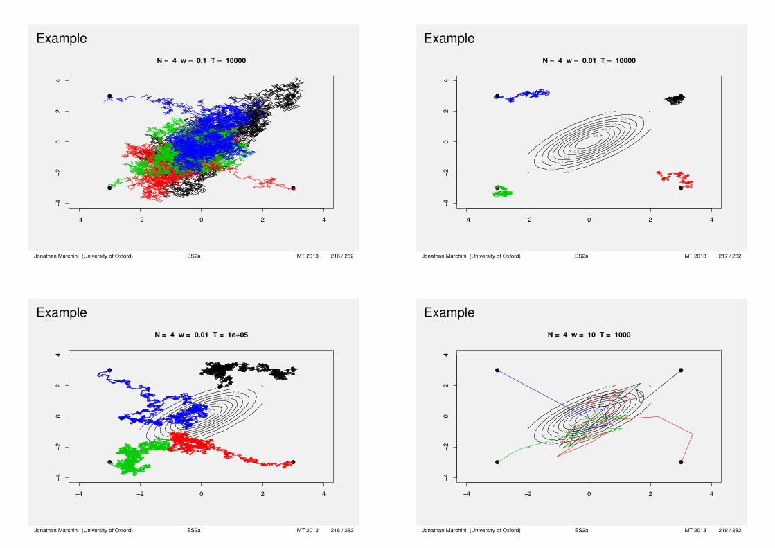
Example

N = 4 w = 0.1 T = 10000

−4 −2 0 2 4

−4−2

02

4


Example

N = 4 w = 0.01 T = 10000

−4 −2 0 2 4

−4−2

02

4


Example

N = 4 w = 0.01 T = 1e+05

−4 −2 0 2 4

−4−2

02

4


Example

N = 4 w = 10 T = 1000

−4 −2 0 2 4

−4−2

02

4


The Metropolis-Hastings algorithmThe Metropolis-Hastings (MH) algorithm generalises the Metropolisalgorithm in two ways

1 The proposal distribution does not need to be symmetric i.e. wecan have

q(θ′|θ) 6= q(θ|θ′)

2 To correct for any asymmetry in the jumping rule the acceptanceratio becomes

α(θ′|θ) = min{

1,π(θ′|x)/q(θ′|θ)

π(θ|x)/q(θ|θ′)

}= min

{1,π(θ′|x)

π(θ|x)

q(θ|θ′)q(θ′|θ)

}

Allowing asymmetric proposals can help the chain to converge faster.Exercise Prove detailed balance for the MH algorithm.


Choosing a proposal distribution

A good proposal distribution has the following properties1 For any θ, it is easy to sample from q(θ′|θ).2 It is easy to compute the acceptance ratio.3 Each proposal goes a reasonable distance in the parameter

space (otherwise the chain moves too slowly).4 The proposals are not rejected too often (otherwise the chain

spends too much time at the same positions).


The Gibbs samplerA Gibbs sampler is a particular type of MCMC algorithm that has beenfound to be very useful in high dimensional problems.

Suppose we wish to sample from π(θ) where θ = (θ1, . . . , θd ). Eachiteration of the Gibbs sampler occurs as follows

1 An ordering of the d components of θ is chosen.2 For each component in this ordering, θj say, we draw a new value

is sampled from the full conditional distribution given all theother components of θ.

θtj ∼ π(θj |θt−1

−j )

where θt−1−j represents all the components of θ, except the for θj , at

their current values

θt−1−j = (θt

1, . . . , θtj−1, θ

t−1j+1 , . . . , θ

t−1d ).


Example

Consider a single observation y = (y1, y2) from a bivariate Normaldistribution with unknown mean θ = (θ1, θ2) and known covariance

Σ =

(1 ρρ 1

). With a uniform prior on θ, the posterior distribution is

θ|y ∼ N(y ,Σ)

In this case the posterior is tractable but we will consider how toconstruct a Gibbs sampler.

We need the two conditional distributions π(θ1|θ2, y) and π(θ2|θ1, y).


Example

π(θ1|θ2, y) ∝ π(θ1, θ2|y)

∝ exp

{− 1

2(θ − y)T Σ−1(θ − y)

}

∝ exp

{− 1

2(1− ρ2)

(θ1 − y1θ2 − y2

)T ( 1 −ρ−ρ 1

)(θ1 − y1θ2 − y2

)}

= exp

{(θ1 − y1)2 + 2ρ(θ1 − y1)(θ2 − y2) + (θ2 − y2)2

}

∝ exp

{− 1

2(1− ρ2)(θ1 − (y1 + ρ(θ2 − y2)))2

}

⇒ θ1|θ2, y ∼ N(y1 + ρ(θ2 − y2),1− ρ2)

Similarly,θ2|θ1, y ∼ N(y2 + ρ(θ1 − y1),1− ρ2)


Example

N = 1 T = 1000

−4 −2 0 2 4

−4−2

02

4


Deriving full conditional distributions

The Gibbs sampler requires us to be able to obtain the full conditionaldistributions of all components of the parameter vector θ.

To determine π(θj |θt−1−j ) we write down the posterior distribution and

consider it as a function of θj .

If we are lucky then we will be able to ‘spot’ the distribution for θj |θt−1−j

(using conjugate priors often helps).

If the full conditional is not of a nice form then this component could besampled using rejection sampling or a MH update could be usedinstead of a Gibbs update.


Gibbs sampling and Metropolis-HastingsGibbs sampling can be viewed as a special case of the MH algorithmwith proposal distributions equal to the full conditionals.

The MH acceptance ratio is min(1, r) where

r =π(θ′)/q(θ′|θt−1)

π(θt−1)/q(θt−1|θ′)

We have θt−1 = (θ1, . . . , θj , . . . , θd ) = (θj , θt−1−j ) and we use proposal

q(θ′|θt−1) = π(θ′j |θt−1−j )

so that θ′ = (θ1, . . . , θ′j , . . . , θd ) = (θ′j , θ

t−1−j ) and

q(θt−1|θ′) = π(θj |θt−1−j )

.Jonathan Marchini (University of Oxford) BS2a MT 2013 227 / 282

Gibbs sampling and Metropolis-HastingsThen the MH acceptance ratio is min(1, r) where

r =π(θ′)/q(θ′j |θt−1)

π(θt−1)/q(θt−1j |θ′)

=π(θ′)/π(θ′j |θ

t−1−j )

π(θt−1)/π(θj |θt−1−j )

But the numerator can be simplified

π(θ′)

π(θ′j |θt−1−j )

=π(θ′j , θ

t−1−j )

π(θ′j |θt−1−j )

= π(θt−1−j )

Similarly the denominator can be simplified

π(θt−1)

π(θj |θt−1−j )

=π(θj , θ

t−1−j )

π(θj |θt−1−j )

= π(θt−1−j )

So we have r =π(θ′)/π(θ′j |θ

t−1−j )

π(θt−1)/π(θj |θt−1−j )

=π(θt−1−j )

π(θt−1−j )

= 1

Thus, every proposed move is accepted.Jonathan Marchini (University of Oxford) BS2a MT 2013 228 / 282

Lecture 14 : Variational Bayes


A key quantity in Bayesian inference is the marginal likelihood of a setof data D given a model M

P(D|M) =

∫P(D|θ,M)P(θ|M)dθ

where θ are the parameters of the model and P(θ|M) is the prior onthe parameters of the model.

The integral required to calculate the marginal likelihood of a givenmodel is not always tractable for some models, so an approximationcan be desirable.

Variational Bayes (VB) is one possibility, that has become reasonablypopular recently.


Variational Bayes

The idea of VB is to find an approximation Q(θ) to a given posteriordistribution P(θ|D,M). That is

Q(θ) ≈ P(θ|D,M)

where θ is the vector of parameters of the model M.

We then use Q(θ) to approximate the marginal likelihood. In fact, whatwe do is find a lower bound for the marginal likelihood.

Question How to find a good approximate posterior Q(θ)?


Kullback-Liebler (KL) divergenceThe strategy we take is to find a distribution Q(θ) that minimizes ameasure of ’distance’ between Q(θ) and the posterior P(θ|D,M).

Definition The Kullback-Leibler divergence KL(q|p) between twodistributions q(x) and p(x) is

KL(q|p) =

∫log[q(x)

p(x)

]q(x)dx

0 5 10 15 20

0.00

0.05

0.10

0.15

0.20

x

dens

ity

q(x)p(x)

0 5 10 15 20−

0.02

0.02

0.06

0.10

x

q(x)

* lo

g(q(

x)/p

(x))

Exercise KL(q|p) ≥ 0 and KL(q|p) = 0 iff q = p.Jonathan Marchini (University of Oxford) BS2a MT 2013 232 / 282

N(µ, σ2) approximations to a Gamma(10,1)

0 5 10 15 20

0.00

0.10

0.20

µ = 10,σ2 = 4,KL = 0.223

x

dens

ity

0 5 10 15 20

0.00

0.10

0.20

µ = 9.11,σ2 = 3.03,KL = 0.124

x

dens

ity

0 5 10 15 20

0.00

0.10

0.20

µ = 13,σ2 = 2.23,KL = 0.347

x

dens

ity

0 5 10 15 20

0.00

0.10

0.20

µ = 9,σ2 = 2,KL = 0.386

x

dens

ity


We consider the KL divergence betweem Q(θ) and P(θ|D,M)

KL(Q(θ)||P(θ|D,M)) =

∫log[ Q(θ)

P(θ|D,M)

]Q(θ)dθ

=

∫log[Q(θ)P(D|M)

P(θ,D|M)

]Q(θ)dθ

= log P(D|M)−∫

log[p(θ,D|M)

Q(θ)

]Q(θ)dθ

The log marginal likelihood can then be written as

log P(D|M) = F (Q(θ)) + KL(Q(θ)||P(θ|D,M)) (1)

where F (Q(θ)) =∫

log[

P(θ,D|M)Q(θ)

]Q(θ)dθ.

Note Since KL(q|p) ≥ 0 we have that

log P(D|M) ≥ F (Q(θ))

so that F (Q(θ)) is a lower bound on the log-marginal likelihood.Jonathan Marchini (University of Oxford) BS2a MT 2013 234 / 282

The mean field approximation

We now need to ask what form that Q(θ) should take?

The most widely used approximation is known as the mean fieldapproximation and assumes only that the approximate posterior hasa factorized form

Q(θ) =∏

i

Q(θi)

The VB algorithm iteratively maximises F (Q(θ)) with respect to thefree distributions, Q(θi), which is coordinate ascent in the functionspace of variational distributions.

We refer to each Q(θi) as a VB component.

We update each component Q(θi) in turn keeping Q(θj) j 6= i fixed.


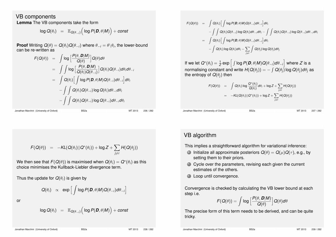
VB componentsLemma The VB components take the form

log Q(θi) = EQ(θ−i )

(log P(D, θ|M)

)+ const

Proof Writing Q(θ) = Q(θi)Q(θ−i) where θ−i = θ\θi , the lower-boundcan be re-written as

F (Q(θ)) =

∫log[P(θ,D|M)

Q(θ)

]Q(θ)dθ

=

∫ ∫log[ P(θ,D|M)

Q(θi )Q(θ−i )

]Q(θi )Q(θ−i )dθidθ−i

=

∫Q(θi )

[ ∫log P(D, θ|M)Q(θ−i )dθ−i

]dθi

−∫ ∫

Q(θi )Q(θ−i ) log Q(θi )dθ−idθi

−∫ ∫

Q(θi )Q(θ−i ) log Q(θ−i )dθ−idθi


F (Q(θ)) =

∫Q(θi )


]dθi

−∫ ∫

Q(θi )Q(θ−i ) log Q(θi )dθ−i dθi −∫ ∫

Q(θi )Q(θ−i ) log Q(θ−i )dθ−i dθi

=

∫Q(θi )


]dθi

−∫

Q(θi ) log Q(θi )dθi −∑j 6=i

∫Q(θj ) log Q(θj )dθj

If we let Q∗(θi) = 1Z exp

[ ∫log P(D, θ|M)Q(θ−i)dθ−i

]where Z is a

normalising constant and write H(Q(θj)) = −∫

Q(θj) log Q(θj)dθj asthe entropy of Q(θj) then

F (Q(θ)) =

∫Q(θi ) log

Q∗(θi )

Q(θi )dθi + log Z +

∑j 6=i

H(Q(θj ))

= −KL(Q(θi )||Q∗(θi )) + log Z +∑j 6=i

H(Q(θj ))


F (Q(θ)) = −KL(Q(θi)||Q∗(θi)) + log Z +∑j 6=i

H(Q(θj))

We then see that F (Q(θ)) is maximised when Q(θi) = Q∗(θi) as thischoice minimises the Kullback-Liebler divergence term.

Thus the update for Q(θi) is given by

Q(θi) ∝ exp[ ∫

log P(D, θ|M)Q(θ−i)dθ−i

]or

log Q(θi) = EQ(θ−i )

(log P(D, θ|M)

)+ const


VB algorithm

This implies a straightforward algorithm for variational inference:1 Initialize all approximate posteriors Q(θ) = Q(µ)Q(τ), e.g., by

setting them to their priors.2 Cycle over the parameters, revising each given the current

estimates of the others.3 Loop until convergence.

Convergence is checked by calculating the VB lower bound at eachstep i.e.

F (Q(θ)) =

∫log[P(θ,D|M)

Q(θ)

]Q(θ)dθ

The precise form of this term needs to be derived, and can be quitetricky.


Example 1Consider applying VB to the hierarchical model

Di ∼ N(µ, τ−1) i = 1, . . . ,P, µ ∼ N(m, (τβ)−1) τ ∼ Γ(a,b)

Note We are using a prior of the form π(τ, µ) = π(µ|τ)π(τ).

Let θ = (µ, τ) and assume Q(θ) = Q(µ)Q(τ).

We will use notation 〈θi〉 = EQ(θ−i )θi .

The log joint density is

log P(D, θ|M) =P2

log τ − τ

2

P∑i=1

(Di − µ)2 +12

log τ − τβ

2(µ−m)2

+(a− 1) log τ − bτ + K


log P(D, θ|M) =P2

log τ − τ

2

P∑i=1

(Di − µ)2 +12

log τ − τβ

2(µ−m)2

+(a− 1) log τ − bτ + K

We can derive the VB updates one at a time. We start with Q(µ). NoteWe just need to focus on terms involving µ.

log Q(µ) = EQ(τ)

(log P(D, θ|M)

)+ C

= −〈τ〉2

( P∑i=1

(Di − µ)2 − β(µ−m)2)

+ C

where 〈τ〉 = EQ(τ)(τ). We will be able to determine 〈τ〉 when we derivethe other component of the approximate density, Q(τ).


We can see this log density has the form of a normal distribution

log Q(µ) = −〈τ〉2

( P∑i=1

(Di − µ)2 − β(µ−m)2)

+ C

= −β′

2(µ−m′)2

where

β′ = (β + P) 〈τ〉

m′ = β′−1(βm +

P∑i=1

Di

)Thus Q(µ) = N(µ|m′, β′−1).


log P(D, θ|M) =P2

log τ − τ

2

P∑i=1

(Di − µ)2 +12

log τ − τβ

2(µ−m)2

+(a− 1) log τ − bτ + K

The second component of the VB approximation is derived as

log Q(τ) = EQ(µ)

(log P(D, θ|M)

)+ C

= ((P + 1)/2 + a− 1) log τ − τ

2

⟨P∑

i=1

(Di − µ)2

⟩

−τ2

⟨β(µ−m)2

⟩+ C


We can see this log density has the form of a gamma distribution

log Q(τ) = ((P + 1)/2 + a− 1) log τ − τ

2

⟨P∑

i=1

(Di − µ)2

⟩

−τ2

⟨β(µ−m)2

⟩+ C

which is Γ(a′,b′) where

a′ = a + (P + 1)/2

b′ = b +12

( P∑i=1

D2i − 2〈µ〉+ P〈µ2〉

)+β

2

(m2 − 2〈µ〉+ 〈µ2〉

)


So overall we have1 Q(µ) = N(µ|m′, β′−1) where

β′ = (β + P) 〈τ〉 (2)

m′ = β′−1(βm +

P∑i=1

Di

)(3)

2 Q(τ) = Γ(τ |a′,b′) where

a′ = a + (P + 1)/2

b′ = b +12

( P∑i=1

D2i − 2〈µ〉+ P〈µ2〉

)+β

2

(m2 − 2〈µ〉+ 〈µ2〉

)To calculate these we need

〈τ〉 =a′

b′〈µ〉 = m′

〈µ2〉 = β′−1 + m′2


Example 1For this model the exact posterior was calculate in Lecture 6.

π(τ, µ | D) ∝ τα′−1 exp[−τ{

b′ +β′

2(m′ − µ)2

}]where

a′ = a +P + 1

2

b′ = b +12

∑(Di − D)2 +

12· Pβ

P + β(D −m)2

β′ = β + P

m′ = β′−1(βm +P∑

i=1

Di)

We note some similarity between the VB updates and the trueposterior parameters.


We can compare the true and VB posterior when applied to a realdataset. We see that VB approximations underestimate posteriorvariances.

−10 −5 0 5 10 15

0.0

0.5

1.0

1.5

2.0

µ

Den

sity

True posteriorVB posterior

0 2 4 6 8

0.0

0.5

1.0

1.5

2.0

2.5

3.0

o

Den

sity

True posteriorVB posterior


General comments

The property of VB underestimating the variance in the posterioris a general feature of the method, when there exists correlationbetween the θi ’s in the posterior, which is usually the case. Thismay not be important if the purpose of inference is modelcomparison i.e. comparing the approximate marginal likelihoodsbetween models.VB is often much, much faster to implement than MCMC or othersampling based methods.The VB updates and lower bound can be tricky to derive, andsometime further approximation is needed.The VB algorithm will find a local mode of the posterior, so careshould be taken when the posterior is thought/known to bemulti-modal.


Laplace’s methodConsider the integral ∫

eNf (x)dx

Expanding f (x) around a maximum point x0 we have

f (x) ≈ f (x0) + f ′(x0)(x − x0) +12

f ′′(x0)(x − x0)2

= ≈ f (x0)− 12|f ′′(x0)|(x − x0)2

and we can approximate the integral as∫eNf (x)dx ≈ eNf (x0)

∫exp

{− N

2|f ′′(x0)|(x − x0)2

}dx

Comparing to a normal pdf we have∫eNf (x)dx ≈ eNf (x0)(2π)

12 N−

12 |f ′′(x0)|−

12


Laplace’s method

For a d-dimensional function the analogue of this result is∫eNf (x)dx ≈ eNf (x0)(2π)

d2 N−

d2 |f ′′(x0)|−

12

where |f ′′(x0)| is the determinant of the Hessian of the functionevaluated at x0.


Laplace approximation

We apply Laplace’s method to the integral that is the marginallikelihood in Bayesian inference, as follows

P(θ|D,M) ∝∫

P(D|θ,M)P(θ|M)dθ

=

∫exp

{N( 1

Nlog P(D|θ,M) +

1N

log P(θ|M))}

dθ

here we have

f (x) =1N

log P(D|θ,M) +1N

log P(θ|M)


Laplace approximation

We let θ be the (vector) value of θ that maximizes the posterior

θ = arg maxθ

P(θ|D,M)

This is known as the maximum a posteriori (MAP) estimate of θ.

This leads to

log P(θ|D,M) ≈ log P(D|θ,M)+log P(θ|M)+d2

log 2π+12

log |f ′′(θ)−1|−d2

log N


Bayesian Information Criterion (BIC)

The Bayesian Information Criterion (BIC) takes the approximation onestep further, essentially by minimizing the impact of the prior.

Firstly, the MAP estimate θ is replaced by the MLE θ, which isreasonable if the prior has a small effect.

Secondly, BIC only retains the terms that vary in N, sinceasymptotically the terms that are constant in N do not matter.

Dropping the constant terms we get,

log P(θ|D,M) ≈ log P(D|θ,M)− d2

log N


Lecture 15 : The EM algorithm


An expectation-maximization (EM) algorithm is an iterative method forfinding maximum likelihood or maximum a posteriori (MAP) estimatesof parameters in statistical models, where the model depends onunobserved latent variables. So called ’missing data’ problems arewidespread in many application areas of statistics.

We will consider the general set up where

X = Observed dataZ = Missing or unobserved dataθ = Model parameters

`(θ) = log L(θ; X )


Example

Suppose we observed data X1, . . . ,XM from the following model

p(Zi = 1) = p(Zi = 2) =12, Xi |Zi ∼ N(θZi ,1)

So we observe the Xi ’s but not the Zi ’s or θ and want to estimate θ.

x

Fre

quen

cy

0 2 4 6

02

46

810

Note If we knew the Zi ’s this would be an easy problem, but wedon’t...hence the need for the EM algorithm.


Overview of EM algorithmThe EM algorithm is an iterative algorithm for maximising thelog-likelihood `(θ) that proceeds as follows

1 Set t = 0 and pick a initial value θt .2 E-Step Calculate the expected log-likelihood of the ’full data’

likelihoodEp(Z |X ,θt )

[log P(X ,Z |θ)

]where the expectation is wrt p(Z |X , θt ) i.e. the conditionaldistribution of the missing data Z given and observed data X andθt .

3 M-Step Set θt+1 = arg maxθ Ep(Z |X ,θt )

[log P(X ,Z |θ)

]4 Iterate steps 2 and 3 until convergence.

Question Why does this work?


`(θ) = log P(X |θ) = logP(X ,Z |θ)

P(Z |X , θ)= log P(X ,Z |θ)− log P(Z |X , θ)

Now take expectations wrt to a distribution q(Z )

`(θ) =

∫log P(X ,Z |θ)q(Z )dZ −

∫log P(Z |X , θ)q(Z )dZ

=

∫log P(X ,Z |θ)q(Z )dZ −

∫log q(Z )q(Z )dz

+

∫log q(Z )q(Z )dz −

∫log P(Z |X , θ)q(Z )dZ

= Eq(Z )

[log P(X ,Z |θ)

]+ H(q(Z )) + KL(q(Z )|P(Z |X , θ))

`(θ) ≥ Eq(Z )

[log P(X ,Z |θ)

]+ H(q(Z ))

where H(q(Z )) = −∫

log q(Z )q(Z )dz is known as the Entropy of q(Z ).


E-StepNow set q(Z ) = P(Z |X , θt ). Then we have

`(θ) ≥ EP(Z |X ,θt )

[log P(X ,Z |θ)

]+ H(q(Z ))

with equality at θ = θt i.e. we have a lower bound for `(θ).

ℓ θ( )

θt


M-StepWe then obtain an updated estimate θt+1 by maximizing this lowerbound

θt+1 = arg maxθ

EP(Z |X ,θt )

[log P(X ,Z |θ)

]since H(q(Z )) is not a function of θ.

ℓ θ( )

θt θt+1


ExampleSuppose we observed data X1, . . . ,XM from the following model

p(Zi = 1) = p(Zi = 2) =12, Xi |Zi ∼ N(θZi ,1)

So we observe the Xi ’s but not the Zi ’s or θ and want to estimate θ.

x

Fre

quen

cy

0 2 4 6

02

46

810


The log-likelihood is

`(θ) = log P(X |θ) = logM∏

i=1

2∑k=1

P(xi |zi = k , θ)p(zi = k)

The full data likelihood and it’s logarithm are given by

P(X ,Z |θ) =M∏

i=1

P(xi |zi , θ)p(zi) =M∏

i=1

N(xi : θzi ,1) · 12

log P(X ,Z |θ) = −12

M∑i=1

(xi − θzi)2 + K


E-Step For θt we then calculate the conditional distribution of themissing data P(Z |X , θt ). This can be done one Zi at a time.

pikt = P(Zi = k |Xi , θt ) ∝ exp(− 1

2(xi − kθt )

2)

Then calculate the expectation of the log of the full data likelihood

E[

log P(X ,Z |θ)]

= −12

M∑i=1

2∑k=1

(xi − θk)2pikt

= −12

M∑i=1

(xi − θ)2pi1t + (xi − 2θ)2pi2t

= −12θ2∑

i

(pi1t + 4pi2t ) + θ∑

i

xi(pi1t + 2pi2t ) + C


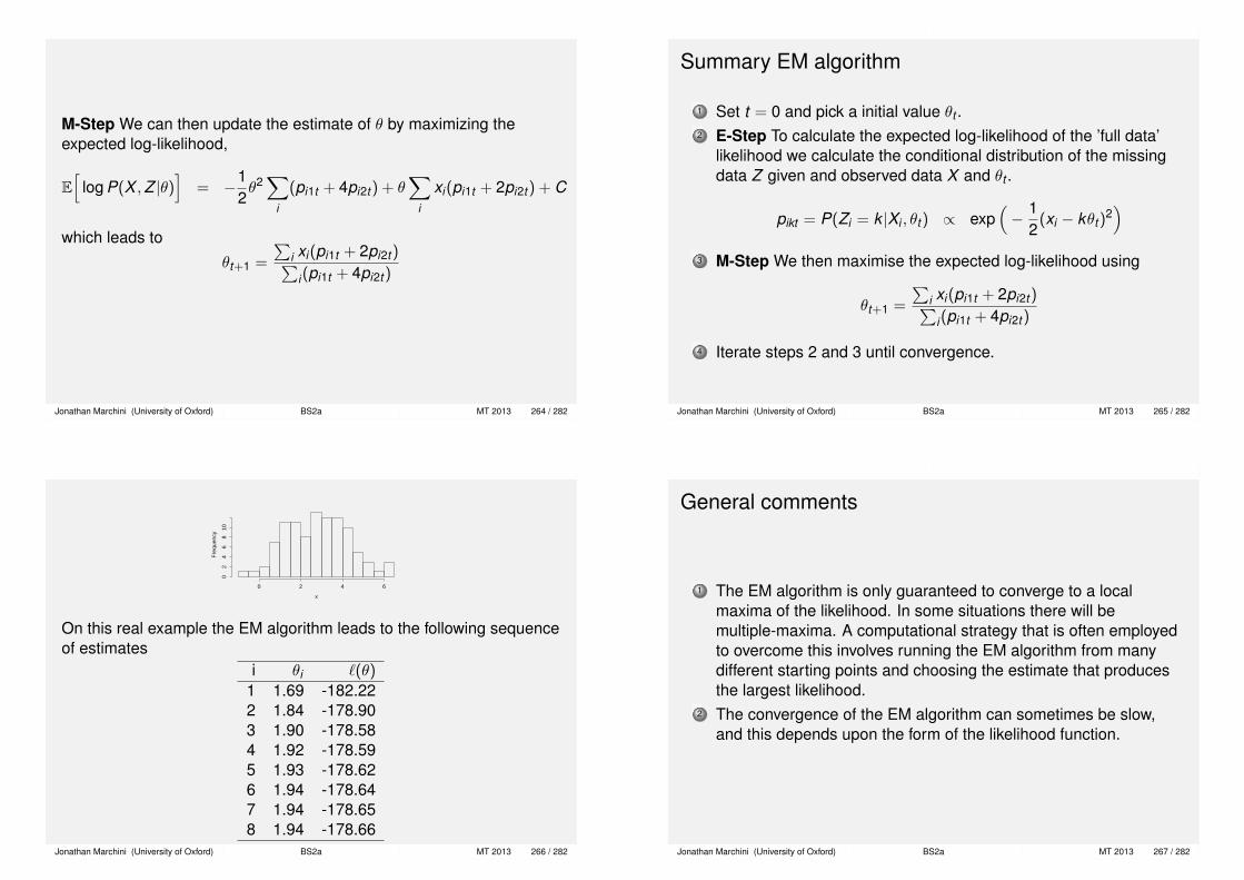
M-Step We can then update the estimate of θ by maximizing theexpected log-likelihood,

E[

log P(X ,Z |θ)]

= −12θ2∑

i

(pi1t + 4pi2t ) + θ∑

i

xi(pi1t + 2pi2t ) + C

which leads toθt+1 =

∑i xi(pi1t + 2pi2t )∑

i(pi1t + 4pi2t )


Summary EM algorithm

1 Set t = 0 and pick a initial value θt .2 E-Step To calculate the expected log-likelihood of the ’full data’

likelihood we calculate the conditional distribution of the missingdata Z given and observed data X and θt .

pikt = P(Zi = k |Xi , θt ) ∝ exp(− 1

2(xi − kθt )

2)

3 M-Step We then maximise the expected log-likelihood using

θt+1 =

∑i xi(pi1t + 2pi2t )∑

i(pi1t + 4pi2t )

4 Iterate steps 2 and 3 until convergence.


x

Fre

quen

cy

0 2 4 6

02

46

810

On this real example the EM algorithm leads to the following sequenceof estimates

i θi `(θ)

1 1.69 -182.222 1.84 -178.903 1.90 -178.584 1.92 -178.595 1.93 -178.626 1.94 -178.647 1.94 -178.658 1.94 -178.66


General comments

1 The EM algorithm is only guaranteed to converge to a localmaxima of the likelihood. In some situations there will bemultiple-maxima. A computational strategy that is often employedto overcome this involves running the EM algorithm from manydifferent starting points and choosing the estimate that producesthe largest likelihood.

2 The convergence of the EM algorithm can sometimes be slow,and this depends upon the form of the likelihood function.


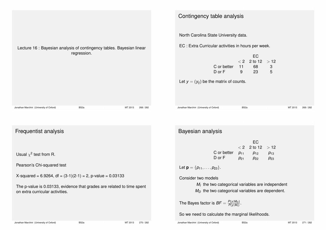
Lecture 16 : Bayesian analysis of contingency tables. Bayesian linearregression.


Contingency table analysis

North Carolina State University data.

EC : Extra Curricular activities in hours per week.

EC< 2 2 to 12 > 12

C or better 11 68 3D or F 9 23 5

Let y = (yij) be the matrix of counts.


Frequentist analysis

Usual χ2 test from R.

Pearson’s Chi-squared test

X-squared = 6.9264, df = (3-1)(2-1) = 2, p-value = 0.03133

The p-value is 0.03133, evidence that grades are related to time spenton extra curricular activities.


Bayesian analysis

EC< 2 2 to 12 > 12

C or better p11 p12 p13D or F p21 p22 p23

Let p = {p11, . . . ,p23}.

Consider two modelsMI the two categorical variables are independent

MD the two categorical variables are dependent.

The Bayes factor is BF = P(y |MD)P(y |MI)

.

So we need to calculate the marginal likelihoods.


The Dirichlet distributionDirichlet integral∫

z1+···+zk =1zν1−1

1 · · · zνk−1k dz1 · · · dzk =

Γ(ν1) · · · Γ(νk )

Γ(∑νi)

Dirichlet distribution

Γ(∑νi)

Γ(ν1) · · · Γ(νk )zν1−1

1 · · · zνk−1k , z1 + · · ·+ zk = 1

The means are E[Zi ] = νi/∑νi , i = 1, . . . , k .

A representation that makes the Dirichlet easy to simulate from is thefollowing.

Let W1, . . . ,Wk be independent Gamma (ν1), . . . Gamma (νk ) randomvariables, W =

∑Wi and set Zi = Wi/W , i = 1, . . . , k .


Examples of 3D Dirichlet distributions


Calculating marginal likelihoods

P(y |MD) =

∫p

P(y |p)π(p)dp

=

∫p11+···+p23=1

(|y |y

)∏ij

(pij)yij π(p)dp11 · · · dp23

where (|y |y

)= (∑

yij)!/∏

yij !

Under MD choose a uniform distribution for p i.e. Dirichlet(1, . . . ,1)

⇒ π(p) = Γ(RC), p11 + · · ·+ p23 = 1


Calculating marginal likelihoods

P(y |MD) =

(|y |y

)Γ(RC)

∫p11+···+p23=1

∏ij

(pij)yij dp11 · · · dp23

=

(|y |y

)Γ(RC)

∏Γ(yij + 1)

Γ(|y |+ RC)

=

(|y |y

)D(y + 1)

D(1RC)

whereD(ν) =

∏Γ(νi)/Γ(

∑νi)

and y + 1 denotes the matrix of counts with 1 added to all entries and1RC denotes a vector of length RC with all entries equal to 1.


Calculating marginal likelihoodsUnder MI the probabilities are determined by the marginal probabilitiespr = {p1·,p2,·} and pc = {p·1,p·2,p·3}

EC< 2 2 to 12 > 12

C or better p11 p12 p13 p1·D or F p21 p22 p23 p2·

p·1 p·2 p·3

Under MI we have a table where pij = pi·p·j .

Under independence MI the row sums and column sums have aDirichlet distribution (with R=2 and C = 3 respectively)

π(pr ) =Γ(R)∏

Γ(1)p1−1

1· · · · p1−1R· = Γ(R), π(pc) =

Γ(C)∏Γ(1)

p1−1·1 · · · p1−1

·C = Γ(C)


The marginal likelihood under MI is therefore

P(y |MI) =

(|y |y

)∫pr

∫pc

∏ij

(pi·p·j

)yij π(pr )π(pc)dpr dpc

=

(|y |y

)Γ(R)Γ(C)

∫pr

∏i

(pi·)yi· dpr

∫pc

∏j

(p·j)y·j dpc

=

(|y |y

)Γ(R)Γ(C)

∏Γ(yi· + 1)

Γ(|y |+ R)

∏Γ(y·j + 1)

Γ(|y |+ C)

=

(|y |y

)D(yR + 1)D(yC + 1)

D(1R)D(1C)


Bayes FactorCombining the two marginal likelihoods we get the Bayes Factor

BF =P(y |MD)

P(y |MI)=

D(y + 1)D(1R)D(1C)

D(1RC)D(yR + 1)D(yC + 1)

Our data is

11 68 3 829 23 5 37

20 91 8 119

The Bayes factor is

11!68!3!9!23!5!1!2!

124!× 120!121!

5!20!91!8!82!37!= 1.66

which gives modest support against independence.Jonathan Marchini (University of Oxford) BS2a MT 2013 278 / 282

Normal Linear regression model

Model: Response variable y , predictor variables x1, . . . , xk .

E(

yi | β,X ) = β1xi1 + · · ·βkxik , i = 1, . . . ,n

In terms of vectors xi = (xi1, . . . , xik ) and β = (β1, . . . , βk )′,

E(

yi | β,X)

= xiβ

{yi} are conditionally independent given values of the parameters andthe predictor variables.


Normal Linear regression modelAssume that

var(yi | θ,X ) = σ2

where unknown parameters are

θ = (β, σ2)

Assume that the errors

εi = yi − E(

yi | β,X)

are independent with mean 0 and variance σ2.That is

y | β, σ2,X ∼ Nn(Xβ, σ2I)

Bayesian formulation: Assume that (β, σ2) have a non-informative prior

g(β, σ2) ∝ 1σ2


Posterior distribution

q(β, σ2|y) = q(β | y , σ2)q(σ2 | y)

The first density on the right is multivariate normal with mean β andcovariance matrix Vβσ2, where

β = (X ′X )−1X ′y , Vβ = (X ′X )−1

Define the inverse gamma (a,b) density as proportional to

y−a−1 exp{−b/y}

then the marginal posterior of σ2 is inverse gamma ((n − k)/2,S/2),where

S = (y − X β)′(y − X β)


The posterior density comes from a classical factorization of thelikelihood

1(2πσ2)n/2 exp

{− 1

2σ2 (y − Xβ)′(y − Xβ)}

knowing that

(y − Xβ)′(y − Xβ) = (y − X β)′(y − X β) + (β − β)′X ′X (β − β)


Foundations of Statistical Inferencemarchini/bs2a/bs2a_4up.pdf · Foundations of Statistical...

Documents

Transcript of Foundations of Statistical Inferencemarchini/bs2a/bs2a_4up.pdf · Foundations of Statistical...