FOUNDATIONS OF GAUGE AND PERSPECTIVE DUALITYmpf/pdfs/2017PerspectiveDuality.pdf · FOUNDATIONS OF...

FOUNDATIONS OF GAUGE AND PERSPECTIVE DUALITY∗

A.Y. ARAVKIN†, J.V. BURKE

‡, D. DRUSVYATSKIY

§, M.P. FRIEDLANDER

¶, AND

K.J. MACPHEE§

Abstract. We revisit the foundations of gauge duality and demonstrate that it can be explainedusing a modern approach to duality based on a perturbation framework. We therefore put gaugeduality and Fenchel-Rockafellar duality on equal footing, including explaining gauge dual variablesas sensitivity measures, and showing how to recover primal solutions from those of the gauge dual.This vantage point allows a direct proof that optimal solutions of the Fenchel-Rockafellar dual of thegauge dual are precisely the primal solutions rescaled by the optimal value. We extend the gaugeduality framework to the setting in which the functional components are general nonnegative convexfunctions, including problems with piecewise linear quadratic functions and constraints that arisefrom generalized linear models used in regression.

Key words. convex optimization, gauge duality, nonsmooth optimization, perspective function

AMS subject classifications. 90C15, 90C25

1. Introduction. Sensitivity of the optimal values and solutions of optimizationproblems, with respect to perturbations in the problem data, is a central concern ofFenchel-Rockafellar duality theory. Lagrange duality can be regarded as a specialcase of this theory, in which perturbations to the data are introduced in a particularmanner. Gauge duality, on the other hand, as introduced in 1987 by Freund [13], wasdeveloped without any reference to sensitivity. It relies instead on a special polaritycorrespondence that exists for nonnegative, positively homogeneous convex functionsthat vanish at the origin; these are known as gauge functions. In 2014, Friedlander,Macedo, and Pong [15] made partial progress towards connecting gauge and Lagrangedualities. In the present work, we show that gauge duality may be regarded as aparticular application of Fenchel-Rockafellar duality theory that is different than theone required for Lagrange duality. This connection provides a useful vantage pointfrom which to develop new algorithms for an important class of convex optimizationproblems. We also describe how gauge duality theory can be extended beyond theoptimization of gauge functions to the optimization of all convex functions that arebounded below. We call this extension perspective duality.

A convenient and fully general formulation for our approach is the problem

minimizex

κ(x) subject to ρ(b−Ax) ≤ σ,(Gp)

where A : Rn → Rm is a linear map, b is an m-vector, and κ and ρ are closed gaugefunctions. For many applications, the function κ is used to regularize the problem inorder to obtain solutions with certain desirable properties. For example, in statisticaland machine-learning applications the regularizer κ is often a nonsmooth, structure-inducing function; e.g. the 1-norm, which is frequently used to encourage sparsity

∗June 18, 2018†Department of Applied Mathematics, University of Washington, Seattle (sasha.aravkin@gmail.

com). Research supported by the Washington Research Foundation Data Science Professorship.‡Seattle, WA ([email protected]). Research supported in part by NSF award DMS-1514559.§Department of Mathematics, University of Washington, Seattle ([email protected]; kmacphee@uw.

edu). Research partially supported by AFOSR YIP award FA9550-15-1-0237.¶

Departments of Computer Science and Mathematics, University of British Columbia, Vancouver,BC, Canada ([email protected]). Research supported by ONR award N00014-16-1-2242.

1

[email protected]

[email protected]

[email protected]

[email protected]

[email protected]

[email protected]

[email protected]

2 ARAVKIN, BURKE, DRUSVYATSKIY, FRIEDLANDER, AND MACPHEE

in the solution. The function ρ may be regarded as a penalty function, such as the2-norm, that measures the degree of misfit between the data b and the linear modelAx, and may reflect a statistical model of the noise in the data b. The perspectiveduality extension enables us to consider optimization problems with a wider rangeof applications by allowing functions κ and ρ that are not positively homogenous,including the Huber function used for robust regression [17], the elastic net used forgroup detection [28], and the logistic loss used for classification [1, 18].

The formulation (Gp) gives rise to two different “dual” problems:

maximizey

〈b, y〉 − σρ◦(y) subject to κ◦(ATy) ≤ 1, and(Ld)

minimizey

κ◦(ATy) subject to 〈b, y〉 − σρ◦(y) ≥ 1.(Gd)

Here ρ◦ and κ◦ are the polars of ρ and κ, which are also gauge functions; see section 2.1for a precise definition. In the important case σ = 0, we interpret σρ◦ as the indicatorfunction of the closure of the domain of ρ◦ (see the discussion in section 2.3). The firstproblem (Ld) is the standard Lagrangian (or Fenchel-Rockafellar) dual, which is thedual problem typically considered in connection with convex optimization problems.Strong duality, reflected in the equality

val (Gp) = val (Ld),

and in the attainment of the optimal value of the Lagrange primal-dual pair, holdsunder mild interiority conditions often referred to as the Slater constraint qualification.The second problem (Gd) is the gauge dual and is less well-known. Under interiorityconditions similar to those required by Lagrange duality, strong duality holds in thegauge duality setting; this is reflected in the analogous equality

1 = val (Gp) · val (Gd),

and in the attainment of the optimal value of the gauge primal-dual pair.In certain contexts, the gauge dual (Gd) can be preferable for computation to

the the primal (Gp) and the Lagrangian dual (Ld), particularly when the polarκ◦ has a special structure. Friedlander and Macedo [14], for example, use gaugeduality to derive an effective algorithm for an important class of low-rank spectraloptimization problems that arise in signal-recovery applications, including phaserecovery and blind deconvolution. Indeed, the effectiveness of numerous convexoptimization algorithms—particularly first-order methods—relies on being able toproject easily onto the constraint set. The appearance of the linear map A in theconstraints of both (Gp) and (Ld) means that such methods may not be efficient,though some recent methods have been proposed that circumvent this difficulty [24].In contrast, the map A appears in the gauge dual (Gd) only in the objective, andcomputing subgradients of this objective only requires subgradients of κ◦, together withthe ability to efficiently implement matrix-vector multiplication. Moreover, typicalapplications occur in the regime m � n. For example, m is often logarithmic inn [6, 7, 11, 26]. Because the dual variables y of (Gd) lie in the much smaller space Rm,projections onto the feasible region may be computed efficiently, depending on thecontext. An example of how an interior method may be used for this purpose is givenin section 5.2.

PERSPECTIVE DUALITY 3

1.1. Approach. This paper has two main goals. The first goal, addressed insection 3, is to show how the foundations of gauge duality can be derived via aperturbation framework pioneered by Rockafellar [20,21], in which the optimal valueand optimal solution depend on parameters to the problem. We follow Rockafellarand Wets [23, 11.H], who consider an arbitrary convex perturbation function F onRn ×Rm that determines how the parameters enter the problem, and define the valuefunctions

(1.1) p(u) := infxF (x, u) and q(v) := inf

yF ?(v, y).

This set-up immediately yields the primal-dual pair

(1.2) p(0) = infxF (x, 0) and p??(0) = sup

y−F ?(0, y) ≡ −q(0).

Fenchel-Rockafellar duality theory flows from an appropriate choice of F . We showthat gauge duality fits equally well into this framework under a judicious choice ofthe perturbation function F , thereby putting Fenchel-Rockafellar and gauge dualitytheories on an equal footing. Strong duality, primal-dual optimality conditions, and aninterpretation of the gauge dual solutions as sensitivity measures—i.e., subgradientsof the value function—quickly follow; cf. section 3.2. These results, in particular,answer an open question posed by Freund in his original work [13], which asked for aninterpretation of gauge dual variables for problems with nonlinear constraints. It alsocompletes a partial analysis by Friedlander et al. [15] on the interpretation of gaugedual variables as sensitivity measures.

This viewpoint allows us to prove a striking relationship between optimal solutionsof the primal and optimal solutions of the Lagrangian dual of the gauge dual: the twocoincide up to scaling by the optimal value (section 3.5). Consequently, Lagrangianprimal-dual methods applied to the gauge dual can be used to recover solutions of theoriginal primal problem. We illustrate this idea in section 7 with an application ofChambolle and Pock’s primal-dual algorithm [8] to a specific problem instance.

The second goal of this paper is to extend the applicability of the gauge dualityparadigm beyond gauges to capture more general convex problems. Section 4 extendsgauge duality to problems involving convex functions that are merely nonnegative, andby an appropriate translation, functions that are bounded from below. The approachis based on using the perspective transform of a convex function [20, p. 35], whichincreases a function’s domain from Rn to Rn+1 and makes it positively homogeneous,enabling the property that is key to the application of gauge duality. We term theresulting dual problem the perspective dual. The perspective-polar transformation,needed to derive the perspective dual problem, is developed in section 4. Concreteillustrations of perspective duality for the family of piecewise linear-quadratic functions,which are often used in data-fitting applications, and for the setting of generalizedlinear models, are given in section 5. We further explore examples of optimalityconditions and primal-from-dual recovery in section 6. Numerical illustrations for acase-study of perspective duals comprise section 7.

2. Notation and assumptions. The derivation of our results relies on standardnotions from convex analysis. Unless otherwise specified, we generally follow Rock-afellar [20] for standard definitions and notation, including domains and epigraphs,relative interiors, convex conjugate functions, subdifferentials, polar sets, etc. In thissection we collect less well-known definitions and notation used throughout the paper,and establish blanket assumptions on the problem data.


Let R := R ∪ {+∞} denote the extended real line, and R+ := {x ∈ R |x ≥ 0}denote the nonnegative extended reals. Let f : Rn → R and g : Rm → R denotegeneral closed convex functions. For a closed convex set C ⊆ Rn, its convex indicatorδC is the closed convex function whose value is zero on C and +∞ otherwise. Letcone C := {λx | λ ≥ 0, x ∈ C } denote the cone generated by C. We often abbreviatefractions such as (1/(2µ)) to (1/2µ).

2.1. The perspective transform. For any convex function f : Rn → R, itsperspective is the function on Rn+1 whose epigraph is the cone generated by theset (epi f) × {1}. Because this transform is not necessarily closed—even when f isclosed—we choose to work with its closure, and redefine the transform as

(2.1) fπ(x, λ) :=

λf(λ−1x) if λ > 0

f∞(x) if λ = 0

+∞ if λ < 0,

where f∞(x) is the recession function of f [20, Theorem 8.5]. A calculus for theperspective transform f 7→ fπ is described by Aravkin, Burke, and Friedlander [2,Section 3.3] and, for the infinite-dimensional case, by Combettes [9,10], where propertiesof the perspective transform are described in detail. We often apply more than onetransformation to a function, and in such cases, the multiple transformations areapplied in the order that they appear; e.g., fπ◦ := (fπ)◦.

2.2. Gauge functions. The following is only a brief description of gauge func-tions. A complete description is given by Rockafellar [20, Section 15].

A convex function κ : Rn → R is called a gauge if it is nonnegative, positivelyhomogeneous, and vanishes at the origin. The symbols κ : Rn → R and ρ : Rm → Rwill always denote closed gauges. The polar of a gauge κ is the function κ◦ defined by

(2.2) κ◦(y) := inf {µ > 0 | 〈x, y〉 ≤ µκ(x), ∀x } ,

which is also a gauge and satisfies κ◦◦ = κ when κ is closed [20, Theorem 15.1]. Forexample, if κ is a norm then κ◦ is the corresponding dual norm. Note the identity

(2.3) epiκ◦ = { (y,−λ) | (y, λ) ∈ (epiκ)◦ } .

It follows directly from (2.2) and positive homogeneity of a gauge function that itspolar can be characterized as the support function to the unit level set, i.e.,

(2.4) κ◦ = δ∗Uκ = sup { 〈u, ·〉 | u ∈ Uκ } where Uκ := {u | κ(u) ≤ 1 } .

Moreover, κ and κ◦ satisfy a Holder-like inequality

(2.5) 〈x, y〉 ≤ κ(x) · κ◦(y) ∀x ∈ domκ, ∀y ∈ domκ◦,

which we refer to as the polar-gauge inequality. The zero level set

Hκ := {u | κ(u) = 0 }

plays a key role when σ = 0. It is straightforward to show that

(2.6) U◦κ = Uκ◦ , U∞κ = Hκ , (domκ)◦ = Hκ◦ , and H◦κ = cl domκ◦

whenever κ is closed, where U∞κ is the recession cone for Uκ [20, Section 8]. We includeproofs of (2.6) in Appendix A.


2.3. Assumptions on the feasible region. Define the following primal anddual feasible sets:

(2.7) Fp := {u | ρ(b− u) ≤ σ } and Fd := { y | 〈b, y〉 − σρ◦(y) ≥ 1 } .

The nonnegativity of ρ implies that the Slater condition can fail when σ = 0, and thusspecial attention is required. In this case, we make the replacement

(2.8) (ρ, σ) ⇒ (δHρ , 1) whenever σ = 0.

This replacement yields a gauge optimization problem whose solution set and optimalvalue coincide with those of (Gp). Observe that because Hρ is a closed convex cone,δHρ = δ∗H◦ρ is a closed gauge that satisfies, by virtue of (2.6), δ◦Hρ = δH◦ρ = δcl dom ρ

◦ .

This motivates the convention made immediately following (Gd) that

(2.9) σρ◦ := δcl dom ρ◦ ≡ δH◦ρ when σ = 0.

The replacement (2.8) allows us to make the useful assumption that σ > inf ρ, whichsignificantly streamlines our analysis. The convention (2.9) also makes sense from anepigraphical perspective, because the functions σρ◦ epigraphically converge to δcl dom ρ

◦

as σ ↓ 0 [23, Proposition 7.4(c)].The gauge primal (Gp) and dual (Gd) problems are said to be feasible, respectively,

if the following intersections are nonempty:

A−1Fp ∩ (domκ) and ATFd ∩ (domκ◦).

Similarly, the primal and dual problems are said to be relatively strictly feasible,respectively, if the following intersections are nonempty:

A−1(riFp

)∩ (ri domκ) and AT riFd ∩ (ri domκ◦).

If the intersections above are nonempty, with interior replacing relative interior, thenwe say that the problems are strictly feasible. We have

riFp =

{{u | b− u ∈ ri dom ρ, ρ(b− u) < σ } if σ > 0

{u | b− u ∈ riHρ } if σ = 0,

riFd =

{{ y | y ∈ ri dom ρ◦, 〈b, y〉 − σρ◦(y) > 1 } if σ > 0

{ y | y ∈ riH◦ρ, 〈b, y〉 > 1 } if σ = 0,

which follows from Rockafellar [20, Theorem 7.6] when σ > 0, and from the conven-tion (2.9) when σ = 0.

We assume throughout that ρ(b) > σ. Otherwise, Fp contains the origin, which isa trivial solution of (Gp). This assumption is consistent with classical applications insignal processing and machine learning, where the corresponding assumption is thatthe data b does not entirely consist of noise.

3. Perturbation analysis for gauge duality. Modern treatment of duality inconvex optimization is based on an interpretation of multipliers as giving sensitivityinformation relative to perturbations in the problem data. No such analysis, however,has existed for gauge duality. In this section we show that for a particular kind ofperturbation, the gauge dual (Gd) can in fact be derived via such an approach.


3.1. General perturbation framework. Our analysis is based on a pertur-bation theory described by Rockafellar and Wets [23, 11.H]. In this section wesummarize the main results from [23] that we need. Fix an arbitrary convex functionF : Rn × Rm → R, and consider the value functions defined by (1.1)–(1.2). Observethe equality q(0) = −p??(0). For example, Fenchel-Rockafellar duality for the problem

(3.1) minimizex

f(Ax) + g(x),

is obtained from the general perturbation theory by setting F (x, u) = f(Ax+u)+g(x).In that case, the primal-dual pair takes the familiar form

p(0) = infx

{f(Ax) + g(x)

}and p??(0) = sup

y

{−f?(−y)− g?(ATy)

}.

Under certain conditions, described in the following theorem, strong duality holds, i.e.p(0) = p??(0), and the optimal values are attained.

Theorem 3.1 (Multipliers and sensitivity [23, Theorem 11.39]). Consider theprimal-dual pair (1.2), where F : Rn × Rm → R is proper, closed, and convex.(a) The inequality p(0) ≥ −q(0) always holds.(b) If 0 ∈ ri dom p, then equality p(0) = −q(0) holds and, if finite, the infimum

q(0) is attained with ∂p(0) = argmaxy −F?(0, y). Similarly, if 0 ∈ ri dom q, then

equality p(0) = −q(0) holds and, if finite, the infimum p(0) is attained with∂q(0) = argminx F (x, 0).

(c) The set argmaxy −F?(0, y) is nonempty and bounded if and only if p(0) is finite

and 0 ∈ int dom p.(d) The set argminx F (x, 0) is nonempty and bounded if and only if q(0) is finite and

0 ∈ int dom q.(e) Optimal solutions are characterized jointly through the conditions

x ∈ argminx F (x, 0)y ∈ argmaxy −F

?(0, y)F (x, 0) = −F ?(0, y)

⇐⇒ (0, y) ∈ ∂F (x, 0) ⇐⇒ (x, 0) ∈ ∂F ?(0, y).

Proof. The only difference between the statement of this theorem and that in [23,Theorem 11.39] is in part (b). Here, we make use of the relative interior rather thanthe interior. Thus, we only prove part (b). Suppose 0 ∈ ri dom p. If p(0) = −∞,then p(0) = −q(0) follows by Part (a). Hence we can assume that p(0) is finite, andconclude that p is proper. By [20, Theorem 23.4], ∂p(0) 6= ∅, and given φ ∈ ∂p(0),

p(0) ≤ p(u)− 〈φ, u〉 = infx

{F (x, u)−

⟨(0φ

),

(xu

)⟩}∀u.

By taking the infimum over u and recognizing the right-hand side as −F ?(0, φ),we deduce that p(0) ≤ −F ?(0, φ) ≤ −q(0). Combining this with Part (a) yieldsp(0) = −F ?(0, φ) = −q(0). Hence φ ∈ argmaxy −F

?(0, y) 6= ∅. Conversely, given anyφ ∈ argmaxy −F

?(0, y), we have

p(0) = −F ?(0, φ) = infx,u

{F (x, u)−

⟨(0φ

),

(xu

)⟩}= inf

u{p(u)− 〈φ, u〉} ≤ p(v)− 〈φ, v〉 ∀ v,

and so φ ∈ ∂p(0). The case 0 ∈ ri dom q follows by an analogous argument.


3.2. A perturbation for gauge duality. We now show that the problems (Gp)and (Gd) constitute a primal-dual pair under the framework set out by Theorem 3.1.The key is to postulate the correct pairing function F . In the derivation below, we showthat the gauge primal-dual pair corresponds to the primal and dual value functions

vp(u) := infµ>0, x

{µ | ρ (b−Ax+ µu) ≤ σ, κ(x) ≤ µ } ,(3.2a)

vd(t, θ) := infy{κ◦(ATy + t) | 〈b, y〉 − σρ◦(y) ≥ 1 + θ } ,(3.2b)

where, as in (Gd), we use the convention described by (2.8) and (2.9). The parametersu and (t, θ) are perturbations to the primal and dual gauge problems, respectively.This perturbation scheme differs significantly from that used in Fenchel-Rockafellarduality—cf. (3.1)—because of the product µu.

We begin by observing that vp(0) is equal to the optimal value of the primal (Gp).Because u and µ appear as a product in this definition, it is convenient to reparametrizethe problem by setting λ := 1/µ and w := x/µ. The positive homogeneity of κ and ρallows us to equivalently phrase the primal value function as

vp(u) = infλ>0, w

{ 1/λ | ρ(λb−Aw + u) ≤ σλ, w ∈ Uκ } .

In particular, this reparameterization shows that the value function vp is convexbecause it is the infimal projection of a convex function, and it is proper when theprimal (Gp) is feasible.

We now construct the function F appearing in Theorem 3.1 associated with thisduality framework. In this construction, we assume that σ > 0, possibly making thereplacement (2.8) if σ = 0. Note that minimizing 1/λ is equivalent to minimizing −λfor λ ≥ 0. Define the convex function F : Rn × R× Rm → R by

F (w, λ, u) := −λ+ δ(epi ρ)×Uκ

Wwλu

, where W :=

−A b Im0 σ 0In 0 0

.Observe that the matrix W is nonsingular.

Because (0, 0, 0) ∈ domF , and κ and ρ are closed, the function F is closed andproper. This pairing function gives rise to the infimal projection problems

(3.3) p(u) := infλ≥0,w

F (w, λ, u) and q(t, θ) := infyF ?(t, θ, y),

which correspond to the general definitions shown in (1.1). Note that the function p isthe reciprocal of vp, as formalized in the following lemma (stated without proof).

Lemma 3.2. Equality vp(u) = −1/p(u) holds provided that vp(u) is nonzero andfinite. Moreover, vp(u) = 0 if and only if p(u) = −∞, and p(u) = 0 if and only ifvp(u) = +∞.

We now compute the conjugate of F , which is needed to derive the dual valuefunction q. By Rockafellar and Wets [23, Theorem 11.23(b)],

F ?(t, θ, y) = cl infz,β,r

δ?(epi ρ)×Uκ

zβr

∣∣∣∣∣∣WT

zβr

=

tθy

+

010

,


where the closure operation cl is applied to the function on the right-hand side withrespect to the argument (t, θ, y). Using the definition of W , the constraint in the

description of F ? is precisely (r − ATz, 〈b, z〉+ σβ, z) = (t, θ + 1, y), and the unique

vector that satisfies these constraints is (z, β, r) = (y, σ−1(θ + 1 − 〈b, y〉), t + ATy).The closure operation is therefore superfluous, and we obtain

F ?(t, θ, y) = δ?(epi ρ)×Uκ

y

σ−1(1 + θ − 〈b, y〉)t+ATy

= δ?epi ρ

(y

σ−1(1 + θ − 〈b, y〉)

)+ δ?Uκ(t+ATy).

Since δ?epi ρ(z1, z2) = δepi ρ◦(z1,−z2) and δ?Uκ = κ◦ by (2.3) and (2.4), this reduces to

F ?(t, θ, y) = δepi ρ◦

(y

−σ−1(1 + θ − 〈b, y〉)

)+ κ◦(t+ATy).

The application of Theorem 3.1 asks that we evaluate these conjugates at (t, θ) = (0, 0),which yields the expression

F ?(0, 0, y) =

{κ◦(ATy) if 〈b, y〉 − σρ◦(y) ≥ 1+∞ otherwise.

Thus, the dual problem

−q(0, 0) = − infyF ?(0, 0, y) = sup

y−F ?(0, 0, y)

recovers, up to a sign change, the required gauge dual problem (Gd) when σ > 0.When σ = 0, we also recover the gauge dual problem (Gd) by making the appropriatesubstitutions (2.8) under the convention (2.9).

This discussion justifies the definition of the dual perturbation function vd(t, θ) :=infy F

?(t, θ, y), which is equivalent to the expression (3.2b). Note that vd(0, 0) is theoptimal value of (Gd). In summary, (−1/vp) and vd, respectively, play the roles of pand q as defined in (3.3). In the application of Theorem 3.1, we identify x with (w, λ),and v with (t, θ).

3.3. Proof of gauge duality. We now use the perturbation framework fromsection 3.2 to prove weak and strong duality results for the gauge duality setting.Theorem 3.4 [15, section 5] is already known, but the proof via perturbation is new.

The following auxiliary result ties the feasibility of the gauge pair (Gp) and (Gd)to the domain of the value function. The proof of this result, which is largely anapplication of the calculus of relative interiors, is deferred to Appendix B.

Lemma 3.3 (Feasibility and domain of the value function). If the primal (Gp)is relatively strictly feasible, then 0 ∈ ri dom p. If the dual (Gd) is relatively strictlyfeasible, then 0 ∈ ri dom vd. The analogous implications, where the ri operator isreplaced by the int operator, hold under strict feasibility (not relative).

The duality relations in the gauge framework follow analogous principles toLagrange duality, except that instead of an additive relationship between the primaland dual optimal values the relationship is multiplicative. The following theoremsummarizes weak and strong duality for gauge optimization.


Theorem 3.4 (Gauge duality [15]). Set νp := vp(0) and νd := vd(0, 0). Then thefollowing relationships hold for the gauge primal-dual pair (Gp) and (Gd).(a) (Basic Inequalities) It is always the case that

(i) (1/νp) ≤ νd and (ii) (1/νd) ≤ νp.

In particular, if νp = 0 (resp. νd = 0), then (Gd) (resp. (Gp)) is infeasible.(b) (Weak duality) If x and y are primal and dual feasible, then

1 ≤ νpνd ≤ κ(x) · κ◦(ATy).

(c) (Strong duality) If the dual (resp. primal) is feasible and the primal (resp. dual) isrelatively strictly feasible, then νpνd = 1 and the gauge dual (resp. primal) attainsits optimal value.

Proof. To simplify notation, in this proof we denote the optimal value of theprimal value function by p0 ≡ p(0).

Part (a). We begin with the inequality (i). Theorem 3.1 guarantees the inequality

(3.4) p0 ≥ − infyF ?(0, 0, y) = −νd.

By Lemma 3.2, whenever νp is nonzero and finite, equality p0 = −1/νp holds, whichtogether with (3.4) yields (i). If, on the other hand, νp = +∞, then (i) is trivial.Finally, if νp = 0, Lemma 3.2 yields p0 = −∞, and hence (3.4) implies νd = +∞,and (i) again holds. Thus, (i) holds always. To establish (ii), it suffices to considerthe case νd = 0. From (3.4) we conclude p0 ≥ 0, that is either p0 = 0 or p0 = +∞.By Lemma 3.2, the first case p0 = 0 implies νp = +∞ and therefore (ii) holds. Thesecond case p0 = +∞ implies that the primal problem is infeasible, that is νp = +∞,and again (ii) holds. Thus (ii) holds always, as required.

Part (b). Because the gauge primal and dual problems are both feasible, νp andνd are nonzero and finite so the result follows from part (a).

Part (c). Suppose the dual is feasible and the primal is relatively strictly feasible. Inparticular, both νp and νd are nonzero and finite by part (a). Hence 1 ≤ νpνd = −νd/p0.On the other hand, by Lemma 3.3 the assumption that the primal is relatively strictlyfeasible implies 0 ∈ ri dom p. This last inequality implies p0 = p(0) is finite, and hencep(·) is proper. Theorem 3.1(b) tells us that p0 = −νd and the infimum in the dual νdis attained. Thus we deduce 1 = νpνd, as claimed.

Conversely, suppose that the primal is feasible and the dual is relatively strictlyfeasible. Then, by Lemma 3.3, 0 ∈ ri dom q . This in turn implies p0 = −νd and thatthe infimum in p(0) is attained. Since the primal is feasible, by Lemma 3.2, p0 isnonzero, and hence 1 = νpνd and the infimum in the primal is attained.

3.4. Gauge optimality conditions. Our perturbation framework can be har-nessed to develop optimality conditions for the gauge pair that relate the primal-dualsolutions to subgradients of the corresponding value function. This yields a version ofparts (b) and (d) in Theorem 3.1 that are specialized to gauge duality.

Theorem 3.5 (Gauge multipliers and sensitivity). The following relationshipshold for the gauge primal-dual pair (Gp) and (Gd).(a) If the primal is relatively strictly feasible and the dual is feasible, then the set of

optimal solutions for the dual is nonempty and coincides with

∂p(0) = ∂(−1/vp)(0).


If it is further assumed that the primal is strictly feasible, then the set of optimalsolutions to the dual is bounded.

(b) If the dual is relatively strictly feasible and the primal is feasible, then the set ofoptimal solutions for the primal is nonempty with solutions x∗ = w∗/λ∗, where

(w∗, λ∗) ∈ ∂vd(0, 0) and λ∗ > 0.

If it is further assumed that the dual is strictly feasible, then the set of optimalsolutions to the primal is bounded.

Proof. Part (a). Because (Gp) is relatively strictly feasible, it follows fromLemma 3.3 that 0 ∈ ri dom p, and because the dual is feasible, p(0) is finite. Theo-rem 3.1 and Lemma 3.2 then imply the conclusion of Part (a). The statement on theboundedness of the set of the optimal solutions to the dual follows from Theorem 3.1.

Part (b). Because (Gd) is relatively strictly feasible, it follows from Lemma 3.3that 0 ∈ ri dom vd, and because the primal is feasible, vd(0) is finite. Theorem 3.1then implies that the optimal primal set is nonempty, and argminw,λ F (w, λ, 0) =∂vd(0, 0). Because the primal and dual problems are feasible, any pair (w∗, λ∗) ∈argminw,λ F (w, λ, 0) must satisfy λ∗ > 0 by Theorem 3.4 and Lemma 3.2. Thus, thisinclusion is equivalent to x∗ = w∗/λ∗ being optimal for the primal problem, withoptimal value 1/λ∗. This proves Part (b). The statement on the boundedness of theset of the optimal solutions to the primal again follows from Theorem 3.1.

We use the sensitivity interpretation given by Theorem 3.5 to develop a set ofnecessary and sufficient optimality conditions that mirror the more familiar KKTconditions from Lagrange duality. For a primal-dual optimal pair (x∗, y∗), the conditionρ◦(y∗) = 0 characterizes a degenerate case when σ > 0 because in that case the primalconstraint is inactive at x∗ (i.e., ρ(b − Ax∗) < σ). On the other hand, the dualconstraint is always active at optimality because the positive homogeneity of the dualobjective and the dual constraint imply 〈b, y∗〉 − σρ◦(y∗) = 1. The full primal-dualoptimality conditions for gauge duality are described in the following theorem.

Theorem 3.6 (Optimality conditions). Suppose both problems of the gauge dualpair (Gp) and (Gd) are relatively strictly feasible, and the pair (x∗, y∗) is primal-dualfeasible. Then (x∗, y∗) is primal-dual optimal if and only if it satisfies the conditions

ρ(b−Ax∗) = σ or ρ◦(y∗) = 0 (primal activity)(3.5a)

〈b, y∗〉 − σρ◦(y∗) = 1 (dual activity)(3.5b)

〈x∗, ATy∗〉 = κ(x∗) · κ◦(ATy∗) (objective alignment)(3.5c)

〈b−Ax∗, y∗〉 = σρ◦(y∗). (constraint alignment)(3.5d)

Proof. First suppose that (x, y) satisfies (3.5a)-(3.5d). By Theorem 3.4, to show

that (x, y) is primal-dual optimal it is sufficient to show that κ(x) · κ◦(ATy) = 1.Add (3.5c) and (3.5d) to obtain

〈b, y〉 = κ(x) · κ◦(ATy) + σρ◦(y).

By combining the above with (3.5b) we obtain κ(x) · κ◦(ATy) = 1, as desired.Suppose now that (x∗, y∗) is primal-dual optimal. We begin by assuming that

σ > 0 and obtain the case σ = 0 by applying the result for the σ > 0 case under thereplacement (2.8). By the positive homogeneity of κ◦ and the optimality of y∗, (3.5b)


holds. Also note that κ(x∗) and κ◦(ATy∗) are both nonzero and finite because of thestrong duality guaranteed by Theorem 3.4.

Define λ∗ := 1/κ(x∗) and w∗ := λ∗x∗, so that κ(w∗) = 1. By Theorem 3.1(e)and Theorem 3.5(b), we must have (0, 0, y∗) ∈ ∂F (w∗, λ∗, 0). Since the primalproblem is relatively strictly feasible, we can apply [20, Theorem 23.9] to deduce thecharacterization

(3.6) ∂F (w, λ, 0) = −

010

+WTN (epi ρ)×Uk

λb−Awσλw

,

where N C(·) denotes the normal cone to a set C. We now consider two cases. First,suppose ρ(λ∗b−Aw∗) = λ∗σ. Then (3.5a) holds, and by straightforward computationsinvolving only (2.4) and the definitions of normal cones and subdifferentials, we have

N (epi ρ)×Uk

λ∗b−Aw∗σλ∗

w∗

= N epi ρ

(λ∗b−Aw∗

σλ∗

)×NUk(w∗),

where

N epi ρ

(λ∗b−Aw∗

σλ∗

)= cone

(∂ρ(λ∗b−Aw∗)× {−1}

)and NUk(w∗) = { v | κ◦(v) ≤ 〈v, w∗〉 }. Substitute these formulas into (3.6) to obtain

∂F (w∗, λ∗, 0) =

v − µATzµ(〈b, z〉 − σ)− 1

µz

∣∣∣∣∣∣ µ ≥ 0, z ∈ ∂ρ(λ∗b−Aw∗), v ∈ NUκ(w∗)

.

We deduce the existence of z∗ ∈ ∂ρ(λ∗b−Aw∗) and µ∗ ≥ 0 such that

y∗ = µ∗z∗(3.7a)

µ∗(〈b, z∗〉 − σ) = 1(3.7b)

κ◦(µ∗ATz∗) ≤ 〈µ∗ATz∗, w∗〉.(3.7c)

Note that µ∗ = 0 cannot satisfy (3.7b), hence (3.7c), together with the polar-gaugeinequality and the fact that κ(w∗) = 1, implies

κ◦(ATy∗) · κ(w∗) = κ◦(ATy∗) ≤ 〈ATy∗, w∗〉 ≤ κ◦(ATy∗) · κ(w∗).

Equality must hold in the above, and dividing through by λ∗ > 0 we see that(3.5c) is satisfied. Finally, we aim to show that (3.5d) holds using the fact thaty∗ ∈ µ∗∂ρ(λ∗b−Aw∗). From the characterization (2.4) of the polar, we have

(3.8) ∂ρ(u) = argmaxy

{ 〈y, u〉 | ρ◦(y) ≤ 1 } .

In particular, this characterization implies 〈y∗/µ∗, λ∗b−Aw∗〉 ≥ 〈0, λ∗b−Aw∗〉 = 0.If ρ(λ∗b−Aw∗) = 0, then by the polar-gauge inequality (2.5) we have

0 ≤ 〈y∗, λ∗b−Aw∗〉 ≤ ρ(λ∗b−Aw∗) · ρ◦(y∗) = 0,


which gives condition (3.5d) after dividing through by λ∗. On the other hand, ifρ(u) > 0 then the set (3.8) is given by { y | ρ(u) = 〈y, u〉, ρ◦(y) = 1 }. Thus whenρ(λ∗b−Aw∗) > 0, we again have 〈y∗/µ∗, λ∗b−Aw∗〉 = ρ◦(y∗/µ∗) · ρ(λ∗b−Aw∗), andmultiplying through by µ∗/λ∗ and applying (3.5a) gives (3.5d).

We have shown the forward implication of the theorem when ρ(λ∗b−Aw∗) = λ∗σ.The other case we need to consider is when ρ(λ∗b−Aw∗) < λ∗σ, or equivalently whenρ(b−Ax∗) < σ. An easy argument (e.g., see [12, Proposition 2.14(iv)]) shows

N epi ρ(λ∗b−Aw∗, λ∗σ) = N dom ρ(λ

∗b−Aw∗)× {0}.

Similar to the first case, we now have

∂F (w∗, λ∗, 0) =

v −ATz〈b, z〉 − 1

z

∣∣∣∣∣∣ z ∈ N dom ρ(λ∗b−Aw∗), v ∈ NUκ(w∗)

.

We deduce that y∗ ∈ N dom ρ(λ∗b − Aw∗) and also that 〈b, y∗〉 = 1 and κ◦(ATy∗) ≤

〈ATy∗, w∗〉. Again, because κ(w∗) = 1, the polar-gauge inequality implies (3.5c) holds.We now show that ρ◦(y∗) = 0 and 〈b−Ax∗, y∗〉 = 0, which, if true, establishes (3.5a)

and (3.5d) are satisfied as well. First note that y∗ ∈ N dom ρ(u) implies y∗ ∈ (dom ρ)◦,which implies ρ◦(y∗) = 0 by (2.6) . Thus, by (3.5b), (3.5c), and the fact that

κ(x∗) · κ◦(ATy∗) = 1 from Theorem 3.4, we have

〈b−Ax∗, y∗〉 = 1− κ(x∗) · κ◦(ATy∗) = 0.

Thus if (x∗, y∗) is primal-dual optimal, then (3.5a)-(3.5d) hold, as claimed. Thisfinishes the proof for σ > 0.

Let us now consider the case when σ = 0 and apply what we have just provedto the pair (Gp) and (Gd) under the replacement (2.8). Then (x∗, y∗) is primal-dualoptimal if and only if the conditions (3.5a)-(3.5d) hold with (ρ, σ) = (δHρ , 1), i.e.,

δH◦ρ(y∗) = 0, 〈x∗, ATy∗〉 = κ(x∗) · κ◦(ATy∗),

〈b, y∗〉 − δH◦ρ(y∗) = 1, 〈b−Ax∗, y∗〉 = 0.

If we combine this with primal feasibility, ρ(b−Ax∗) = 0, and use the identity (2.9)that 0 · ρ◦ = δH◦ρ , then these conditions are equivalent to (3.5a)-(3.5d) for σ = 0, ρ,

and ρ◦ as written above.

The following corollary describes a variation of the optimality conditions outlinedby Theorem 3.6. These conditions assume that a solution y∗ of the dual problem isavailable, and gives conditions that can be used to determine a corresponding solutionof the primal problem. An application of the following result appears in section 6.

Corollary 3.7 (Gauge primal-dual recovery). Suppose that the primal-dualpair (Gp) and (Gd) are each relatively strictly feasible. If y∗ is optimal for (Gd), thenfor any primal feasible x the following conditions are equivalent:(a) x is optimal for (Gp);

(b) 〈x,ATy∗〉 = κ(x) · κ◦(ATy∗) and b−Ax ∈ ∂(σρ◦)(y∗);

(c) ATy∗ ∈ κ◦(ATy∗) · ∂κ(x) and b−Ax ∈ ∂(σρ◦)(y∗),where, by convention, σρ◦ = δcl dom ρ

◦ when σ = 0.


Proof. We use the optimality conditions given in Theorem 3.6. As noted before,by the optimality of y∗ we automatically have equality (3.5b) in the dual constraint.

We first show that (b) implies (a). Suppose (b) holds. Then (3.5c) holds automat-ically. From the characterization (2.4) of the polar, we have

(3.9) σρ◦(y∗) =

σ · supρ(z)≤1

〈y∗, z〉 if σ > 0

δcl dom ρ◦(y∗) if σ = 0

= supρ(z)≤σ

〈y∗, z〉,

where the case σ = 0 uses the convention (2.9). Thus, ∂(σρ◦)(y∗) is the set ofmaximizing elements in this supremum. Because b−Ax ∈ ∂(σρ◦)(y∗), it holds thatρ(b−Ax) ≤ σ. If we additionally use the polar-gauge inequality, we deduce that

σρ◦(y∗) = 〈y∗, b−Ax〉 ≤ ρ(b−Ax) · ρ◦(y∗) ≤ σρ◦(y∗),

and therefore the above inequalities are all tight. Thus conditions (3.5a) and (3.5d)hold, and by Theorem 3.6, (x, y) is a primal-dual optimal pair.

We next show that (a) implies (b). Suppose that x is optimal for (Gp). Then thefirst condition of (b) holds by (3.5c), and (3.5a) and (3.5d) combine to give us

σρ◦(y∗) = ρ(b−Ax) · ρ◦(y∗) = 〈b−Ax, y∗〉.

This implies that z := b−Ax is a maximizing element of the supremum in (3.9), andthus b−Ax ∈ ∂(σρ◦)(y∗).

Finally, to show the equivalence of (b) and (c), note that by the polar-gauge

inequality, 〈x,ATy∗〉 = κ(x) · κ◦(ATy∗) if and only if x minimizes the convex function

κ◦(ATy∗)κ(·)−〈·, ATy∗〉. This, in turn, is true if and only if 0 ∈ κ◦(ATy∗) ∂κ(x)−ATy∗,or equivalently, ATy∗ ∈ κ◦(ATy∗) · ∂κ(x).

3.5. The relationship between Lagrange and gauge multipliers. We nowuse the perturbation framework for duality to establish a relationship between gaugedual and Lagrange dual variables. We begin with an auxiliary result that characterizesthe subdifferential of the perspective function (2.1). Combettes [10, Prop. 2.3(v)]also describes an equivalent formula for the subdifferential, though the derivation andsubsequent form of the expression are very different. The formula in Lemma 3.8 ismore suitable for our purposes.

Lemma 3.8 (Subdifferential of perspective function). Let g : Rn → R be a closedproper convex function. Then for (x, µ) ∈ dom gπ, equality holds:

∂gπ(x, µ) =

{{ (z,−g?(z)) | z ∈ ∂g(x/µ) } if µ > 0

{ (z, γ) | (z,−γ) ∈ epi g?, z ∈ ∂g∞(x) } if µ = 0.

Proof. Recall that the subdifferential of the support function to any nonemptyclosed convex set C is given by ∂δ?C(x) = argmax { 〈z, x〉 | z ∈ C } [20, Theorem 23.5 andCorollary 23.5.3]. By [20, Corollary 13.5.1], gπ = δ?C , where C = { (z, γ) | g?(z) ≤ −γ }is a closed convex set. If (x, µ) ∈ dom gπ, then C is nonempty and

∂gπ(x, µ) = argmax(z,γ)∈C

{ 〈(x, µ), (z, γ)〉 } = argmax(z,γ)∈C

{ 〈z, x〉+ µγ } .

Suppose now that µ > 0. Then

(3.10) sup(z,γ)∈C

{ 〈z, x〉+ µγ } = supz∈dom g

?{ 〈z, x〉 − µg?(z) } = µ ·sup

z∈dom g?{ 〈z, x/µ〉 − g?(z) } .


Using the expression for the subdifferential of a support function, (z, γ) achieves thesupremum of (3.10) if z ∈ ∂g(x/µ) and −γ = g?(z). On the other hand, if µ = 0 then

sup(z,γ)∈C

〈z, x〉 = supz∈dom g

?〈z, x〉 = δ?dom g

?(x) = g∞(x).

Again using the expression for the subdifferential of a support function, (z, γ) achievesthe supremum of (3.10) if and only if z ∈ ∂g∞(x) and (z,−γ) ∈ epi g?.

We now state the main result relating the optimal solutions of (Gp) to the optimalsolutions of the Lagrange dual of (Gd).

Theorem 3.9. Suppose that the gauge dual (Gd) is relatively strictly feasible andthe primal (Gp) is feasible. Let (Lp) denote the Lagrange dual of (Gd), and let νLdenote its optimal value. Then

z∗ is optimal for (Lp) ⇐⇒ z∗/νL is optimal for (Gp).

Proof. We first note that (Lp) can be derived via the framework of Theorem 3.1through the Lagrangian value function

h(w) = infy

{κ◦(ATy + w) + δ〈b,·〉−σρ◦(·)≥1(y)

}.

Here h plays the role of p in Theorem 3.1; cf. [23, Example 11.41]. Strong dualityin Theorem 3.4 guarantees that h(0) is nonzero and finite, and by Lemma 3.3,

(Gd) relatively strictly feasible =⇒ (0, 0) ∈ ri dom vd =⇒ 0 ∈ ri domh.

Thus, it follows from Theorem 3.1 that the optimal points z∗ for (Lp) are characterizedby z∗ ∈ ∂h(0). Note also that h(0) = νL.

On the other hand, by Theorem 3.5(b) the solutions to (Gp) are precisely thepoints w∗/λ∗ such that (w∗, λ∗) ∈ ∂vd(0, 0). Thus to relate the solution sets of (Lp)and (Gp), we must relate ∂h(0) and ∂vd(0, 0).

For θ in a neighborhood of zero and all t, by positive homogeneity of κ◦ and ρ◦

we have

vd(t, θ) = (1 + θ)h

(t

1 + θ

)= inf

y

{(1 + θ)κ◦

(ATy +

t

1 + θ

)+ δ〈b,·〉−σρ◦(·)≥1(y)

}.

Thus by Lemma 3.8, ∂vd(0, 0) = { (z,−h?(z)) | z ∈ ∂h(0) } . However, for z ∈ ∂h(0)the Fenchel-Young equality gives us

0 = 〈0, z〉 = h?(z) + h(0) = h?(z) + νL.

Thus we obtain the convenient description

∂vd(0, 0) = ∂h(0)× {h(0)} = ∂h(0)× {νL}

and the set of optimal solutions for (Gp) is precisely 1νL∂h(0).

4. Perspective duality. We now move on to an extension of the gauge dualityframework, which allows us to consider functions that are not necessarily positivelyhomogeneous, but continue to be nonnegative and convex. (The same frameworkapplies to functions that are bounded below because these can be made nonnegative


by translation.) For the remainder of the paper, consider functions f : Rn → R+ andg : Rm → R+, that are closed, convex and nonnegative over their domains. In thissection we derive and analyze the perspective-dual pair

minimizex

f(x) subject to g(b−Ax) ≤ σ,(Np)

minimizey, α, µ

f ](ATy, α) subject to 〈b, y〉 − σg](y, µ) ≥ 1− (α+ µ).(Nd)

The functions f ] and g] are the polars of the perspective transforms of f and g. Thistransform is a key operation needed to derive perspective duality. In the next sectionwe describe properties of that transform and its application to the derivation of theperspective-dual pair. Throughout this section, we assume that σ > infu g(u) ≥ 0.

4.1. Perspective-polar transform. Given a closed proper convex functionf : Rn → R+, define the perspective-polar transform by f ] := (fπ)◦.

An explicit characterization of the perspective-polar transform is given by

(4.1) f ](z,−ξ) = inf {µ > 0 | 〈z, x〉 ≤ ξ + µf(x), ∀x } .

This representation can be obtained by applying the definition of the gauge polar (2.2)to the perspective transform as follows:

f ](z,−ξ) = inf {µ > 0 | 〈z, x〉 − ξλ ≤ µfπ(x, λ), ∀x,∀λ }= inf {µ > 0 | 〈z, x〉 − ξλ ≤ µλf(x/λ), ∀x, ∀λ > 0 }= inf {µ > 0 | 〈z, λx〉 − ξλ ≤ µλf(x), ∀x, ∀λ > 0 } ,

which yields (4.1) after dividing through by λ. Rockafellar’s extension [20, p.136] ofthe polar gauge transform to nonnegative convex functions that vanish at the origincoincides with f ](z,−1).

The following theorem provides an alternative characterization of the perspective-polar transform in terms of the more familiar Fenchel conjugate f?. It also provides anexpression for the perspective-polar of f in terms of the Minkowski function generatedby the epigraph of the conjugate of f , i.e.,

γepi f?(x, τ) := inf {λ > 0 | (x, τ) ∈ λ epi f? } ,

which is a gauge. Nonnegativity of f is not required for the first part of this result.

Theorem 4.1. For any closed proper convex function f with 0 ∈ dom f , we havefπ?(z,−ξ) = δepi f?(z, ξ). If, in addition, f is nonnegative, f ](z,−ξ) = γepi f?(z, ξ).

Proof. Because of the assumptions on f , we have fπ(x, 0) = lim infλ→0

+ fπ(x, λ)for each x ∈ Rn [20, Corollary 8.5.2]. Thus we obtain the following chain of equalities:

fπ?(z,−ξ) = sup { 〈z, x〉 − λξ − fπ(x, λ) | x ∈ Rn, λ ∈ R }= sup { 〈z, x〉 − λξ − λf(λ−1x) | x ∈ Rn, λ > 0 }= sup { 〈z, λy〉 − λξ − λf(y) | y ∈ Rn, λ > 0 }= sup {λ · supy { 〈z, y〉 − ξ − f(y) } | λ > 0 }= sup {λ(f?(z)− ξ) | λ > 0 } = δepi f?(z, ξ).

This proves the first statement. Now additionally suppose that f is nonnegative.Because fπ is closed, it is identical to its biconjugate, and so fπ(x, λ) = δ?epi f?(x,−λ).


Also, epi f? is closed and convex, and contains the origin because f is nonnegative.Therefore, it follows from [20, Corollary 15.1.2] that

f ](z,−ξ) ≡ fπ◦(z,−ξ) = δ?◦epi f?(z, ξ) = γepi f?(z, ξ).

The following result relates the level sets of the perspective-polar transform to thelevel sets of the conjugate perspective. This result is useful in deriving the constraintsets for certain perspective-dual problems for which there is no closed form for theperspective polar; cf. Example 5.4.

Theorem 4.2 (Level-set equivalence). Let f : Rn → R+ be a nonnegative, closedproper convex function with 0 ∈ dom f . Then, for any (z, ξ, µ) ∈ Rn × R× R,

f ](z, ξ) ≤ µ ⇐⇒ [ 0 ≤ µ and f?π(z, µ) ≤ −ξ ].

Proof. The following chain of equivalences follows from Theorem 4.1:

f ](z, ξ) ≤ µ ⇐⇒ γepi f?(z,−ξ) ≤ µ⇐⇒ inf {λ > 0 | (z,−ξ) ∈ λ epi f? } ≤ µ⇐⇒ inf {λ > 0 | f?(z/λ) ≤ −ξ/λ } ≤ µ⇐⇒ inf {λ > 0 | f?π(z, λ) ≤ −ξ } ≤ µ.

(4.2)

Define α = inf {λ > 0 | f?π(z, λ) ≤ −ξ }.We first show that f ](z, ξ) ≤ µ implies 0 ≤ µ and f?π(z, µ) ≤ −ξ. By (4.2),

0 ≤ α ≤ µ. If α < µ, there exists λ with 0 < λ < µ such that f?π(z, λ) ≤ −ξ. Becausef is nonnegative, µf ≥ λf , and thus (µf)? ≤ (λf)?. In particular,

f?π(z, µ) = (µf)?(z) ≤ (λf)?(z) = f?π(z, λ) ≤ −ξ.

On the other hand, if α = µ, there exists a sequence λk → µ such that f?π(z, λk) ≤ −ξfor each k. Now by the lower semi-continuity of f?π, we obtain

f?π(z, µ) ≤ lim infk→∞

f?π(z, λk) ≤ −ξ.

This establishes the forward implication of the theorem.For the reverse implication, suppose 0 ≤ µ and f?π(z, µ) ≤ −ξ. If 0 < µ, it

follows from (4.2) that f ](z, ξ) ≤ µ. Now suppose otherwise that µ = 0. We want to

show f ](z, ξ) ≤ 0. By hypothesis, (z, 0,−ξ) ∈ epi f?π. Thus there exists a sequence(zk, µk, rk) with limk→∞(zk, µk, rk) = (z, 0,−ξ) and f?π(zk, µk) ≤ rk for all k. Withno loss in generality, we can assume that µk > 0 for all k. Then for each k, we haveµkf

?(zk/µk) ≤ rk for which we have the following equivalences:

µkf?(zk/µk) ≤ rk ⇐⇒ sup

w{ 〈w, zk〉 − µkf(w) } ≤ rk

⇐⇒ 〈w, zk〉 ≤ rk + µkf(w), ∀w ∈ Rn

⇐⇒ µk ≥ inf {λ > 0 | 〈w, zk〉 ≤ rk + λf(w), ∀w ∈ Rn }

⇐⇒(4.1)

µk ≥ f](zk,−rk),

which gives f ](z, ξ) ≤ 0 = µ in the limit, since f ] is closed.


4.1.1. Calculus rules. Two useful calculus rules are now developed that governthe perspective-polar transform when applied to gauge functions and separable sums.

Example 4.3 (Gauge functions). Suppose that f is a closed proper gauge. Then

f ](z, ξ) = f◦(z) + δR−(ξ).

Use expression (4.1) for this derivation. When ξ > 0, take x = 0 in the infimum

in (4.1) to deduce that f ](z, ξ) = +∞. On the other hand, when ξ ≤ 0, the positive

homogeneity of f implies that f ](z, ξ) = f◦(z). We leave the details to the reader.

More generally, if f vanishes at the origin, then f ](z, ξ) = +∞ for all ξ > 0.

Example 4.4 (Separable sums). Suppose that f(x) :=∑ni=1 fi(xi), where each

convex function fi : Rni → R+ is nonnegative. Then a straightforward computationshows that fπ(x, λ) =

∑ni=1 f

πi (xi, λ). Furthermore, taking into account [15, Proposi-

tion 2.4], which expresses the polar of a separable sum of gauges, we deduce

f ](z, ξ) = maxi=1,...,n

f ]i (zi, ξ).

4.2. Derivation of the perspective dual via lifting. We now derive therelationship between the primal and dual problems (Np) and (Nd) by lifting (Np) to anequivalent gauge optimization problem, and then recognizing (Nd) as its gauge dual.

Theorem 4.5 (Gauge lifting of the primal). A point x∗ is optimal for (Np) ifand only if (x∗, 1) is optimal for the gauge problem

(4.3) minimizex,λ

fπ(x, λ) subject to ρ

b11

−A 0

0 10 0

[xλ

] ≤ σ,where ρ(z, µ, τ) := gπ(z, τ) + δ{0}(µ) is a gauge function.

Proof. By definition of fπ, x∗ is optimal for (Np) if and only if the pair (x∗, 1) isoptimal for

minimizex,λ

fπ(x, λ) subject to λ = 1, gπ(b−Ax, 1) ≤ σ.

The following equivalence follows from the definition of ρ:

[λ = 1 and gπ(b−Ax, 1) ≤ σ ] ⇐⇒ ρ(b−Ax, 1− λ, 1) ≤ σ.

Thus we arrive at the constraint expressed in (4.3).

Corollary 4.6 (Gauge dual). Problem (Nd) is the gauge dual of (4.3).

Proof. It follows from the canonical dual pairing (Gp) and (Gd) that the gaugedual of (4.3) is

(4.4)minimizey,α,µ

fπ◦

[AT 0 00 1 0

]yαµ

subject to 〈(y, α, µ), (b, 1, 1)〉 − σρ◦(y, α, µ) ≥ 1.

Because ρ is separable in (z, µ) and β, it follows from [15, Proposition 2.4] that

ρ◦(y, α, µ) = max { gπ◦(y, µ), δ◦{0}(α) } .

Since δ◦{0}(α) is identically zero, the result follows.


The next result generalizes the gauge duality result of Theorem 3.4 to the casewhere f and g are convex and nonnegative but not necessarily gauges. We parallel theconstruction in (2.7), and for this section only redefine the feasible sets by

Fp := {u | g(b− u) ≤ σ }

Fd := { (y, α, µ) | 〈b, y〉 − σg](y, µ) ≥ 1− (α+ µ) } .

Thus, (Np) is relatively strictly feasible if

A−1 riFp ∩ (ri dom f) 6= ∅.

Similarly, (Nd) is relatively strictly feasible if there exists a triple (y, α, µ) such that

(ATy, α) ∈ ri dom f ] and (y, α, µ) ∈ riFd.

Strict feasibility follows the same definitions, where the operation ri is replaced by int.

Theorem 4.7 (Perspective duality). Let νp and νd, respectively, denote theoptimal values of the pair (Np) and (Nd). Then the following relationships hold forthe perspective dual pair (Np) and (Nd).(a) (Basic Inequalities) It is always the case that

(i) (1/νp) ≤ νd and (ii) (1/νd) ≤ νp.

Thus, νp = 0 and νd = 0, respectively, imply that (Nd) and (Np) are infeasible.(a) (Weak duality) If x and (y, α, µ) are primal and dual feasible, then

1 ≤ νpνd ≤ f(x) · f ](ATy, α).

(a) (Strong duality) If the dual (resp. primal) is feasible and the primal (resp. dual)is relatively strictly feasible, then νpνd = 1 and the perspective dual (resp. primal)attains its optimal value.

Proof. Parts (a) and (b) follow immediately from the analogous result in Theo-rem 3.4, together with Theorem 4.5 and Corollary 4.6.

Next we demonstrate that (Np) is relatively strictly feasible if and only if (4.3) isrelatively strictly feasible. By the description of relative interiors of sublevel sets givenin [20, Theorem 7.6], (4.3) is relatively strictly feasible if and only if there exists apoint (x, 1) ∈ ri dom fπ such that

(b−Ax, 0, 1) ∈ ri dom ρ and ρ(b−Ax, 0, 1) = g(b−Ax) < σ.

We now seek a description of ri dom fπ. We have

dom fπ = { (x, µ) | fπ(x, µ) <∞}= cl ({0} ∪ { (x, µ) | µ > 0, f(x/µ) <∞}) = cl cone (dom f × {1}).

By [20, Corollary 6.8.1], the above description yields

ri dom fπ = { (x, µ) | µ > 0, x ∈ µ ri dom f } .

Thus (x, 1) ∈ ri dom fπ if and only if x ∈ ri dom f . Similarly,

dom ρ = { (y, 0, µ) | (y, µ) ∈ dom gπ } ,


and so

ri dom ρ = { (y, 0, µ) | (y, µ) ∈ ri dom gπ } = { (y, 0, µ) | µ > 0, y ∈ µ ri dom g } .

In particular, the condition (b−Ax, 0, 1) ∈ ri dom ρ is equivalent to b−Ax ∈ ri dom g.Thus the conditions for relative strict feasibility of (4.3) and (Np) are identical.

A similar argument verifies that (Nd) is relatively strictly feasible if and only if(4.4) is relatively strictly feasible. Strong duality then follows from relative interiority,Corollary 4.6, Theorem 4.5, and the analogous strong-duality result in Theorem 3.4.

4.3. Optimality conditions. The following result generalizes Theorem 3.5 toinclude the perspective-dual pair.

Theorem 4.8 (Perspective optimality). Suppose (Np) is strictly feasible. Thenthe tuple (x∗, y∗, α∗, µ∗) is perspective primal-dual optimal if and only if

g(b−Ax∗) = σ or g](y∗, µ∗) = 0 (primal activity)

〈b, y∗〉 − σg](y∗, µ∗) = 1− (α∗ + µ∗) (dual activity)

〈x∗, ATy∗〉+ α∗ = f(x∗) · f ](ATy∗, α∗) (objective alignment)

〈b−Ax∗, y∗〉+ µ∗ = g(b−Ax∗) · g](y∗, µ∗). (constraint alignment)

Proof. By construction, x∗ is optimal for (Np) if and only if (x∗, 1) is optimalfor its gauge reformulation (4.3). Apply Theorem 3.5 to (4.3) and the correspondinggauge dual (Nd) to obtain the required conditions.

The following result mirrors Corollary 3.7 for the perspective-duality case.

Corollary 4.9 (Perspective primal-dual recovery). Suppose that the primal(Np) is strictly feasible. If (y∗, α∗, µ∗) is optimal for (Nd), then for any primal feasiblex ∈ Rn, the following conditions are equivalent:(a) x is optimal for (Np);

(b) 〈x,ATy∗〉+ α∗ = f(x) · f ](ATy∗, α∗) and (b−Ax, 1) ∈ σ∂g](y∗, µ∗);(c) ATy∗ ∈ f ](ATy∗, α∗) · ∂f(x) and (b−Ax, 1) ∈ σ∂g](y∗, µ∗).

Proof. By construction, x is optimal for (Np) if and only if (x, 1) is optimal forits gauge reformulation (4.3). Apply Corollary 3.7 to (4.3) and its gauge dual (Nd) toobtain the equivalence of (a) and (b). To show the equivalence of (b) and (c), note

that by the polar-gauge inequality, 〈(x, 1), (ATy∗, α∗)〉 ≤ fπ(x, 1) · f ](ATy∗, α∗) for allx, or equivalently,

〈x,ATy∗〉+ α∗ ≤ f(x) · f ](ATy∗, α∗), ∀x.

The inequality is tight for a fixed x if and only if x minimizes the functionh := f ](ATy∗, α∗)f(·)− 〈·, ATy∗〉 − α∗. This in turn is equivalent to 0 ∈ ∂h(x), or

ATy∗ ∈ f ](ATy∗, α∗) · ∂f(x).

This shows the equivalence of (b) and (c) and completes the proof.

Section 6 illustrates an application of Corollary 4.9 for recovering primal optimalsolutions from perspective-dual optimal solutions.


4.4. Reformulations of the perspective dual. Two reformulations of theperspective dual (Nd) may be useful depending on the functions f and g involved in(Np). First, an important simplification of the perspective dual occurs when one orboth of these functions are gauges.

Corollary 4.10 (Simplification for gauges). If f is a gauge, then a triple(y∗, α∗, µ∗) is optimal for (Nd) if and only if α∗ ≤ 0 and (y∗, µ∗) is optimal for

minimizey,α

f◦(ATy

)subject to 〈b, y〉 − σg](y, µ) ≥ 1− µ.

If, in addition, g is a gauge, then a triple (y∗, α∗, µ∗) is optimal for (Nd) if and onlyif α∗ ≤ 0, µ∗ ≤ 0, and y∗ solves (Gd).

Proof. Follows from the formulas for f ] and g] established in section 4.1.1.

Theorem 4.2 also allows us to express the level sets of g] in terms of its conjugatepolar as in the following corollary.

Corollary 4.11. The point (y∗, α∗, µ∗) is optimal for (Nd) if and only if thereexists a scalar ξ∗ such that (y∗, α∗, µ∗, ξ∗) is optimal for the problem

minimizey,α,µ,ξ

f ](ATy, α)

subject to 〈b, y〉 − σξ = 1− (α+ µ), g?π(y, ξ) ≤ −µ, ξ ≥ 0.

Proof. By introducing the variable ξ := (〈b, y〉+ α+ µ− 1)/σ in (Nd), the resultfollows from Theorem 4.2.

5. Examples: piecewise linear-quadratic and GLM constraints. From acomputational standpoint, the perspective-dual formulation may be an attractivealternative to the original primal problem. The efficiency of this approach requires thatthe dual constraints are in some sense more tractable than those of the primal. Forexample, we may consider the dual feasible set “easy” if it admits an efficient procedurefor projecting onto that set. In this section, we examine two special cases that admittractable dual problems in this sense. The first case is the family of piecewise linearquadratic (PLQ) functions, introduced by Rockafellar [22] and subsequently examinedby Rockafellar and Wets [23, p.440], and Aravkin, Burke, and Pillonetto [3]. Thesecond case is when g is a Bregman divergence arising from a maximum likelihoodestimation problem over a family of exponentially distributed random variables.

For this section only, we will assume for the sake of simplicity that the objective f isa gauge, so that the perspective dual in each of this cases simplifies as in Corollary 4.10.The more general case still applies.

5.1. PLQ constraints. The family of PLQ functions is a large class of convexfunctions that includes such commonly used penalties as the Huber function, theVapnik ε-loss, and the hinge loss. The last two are used in support-vector regressionand classification [3]. PLQ functions take the form

(5.1) g(y) = supu∈U{ 〈u,By + b〉 − 1

2‖Lu‖22 } , U := {u ∈ R` |Wu ≤ w } ,

where g is defined by linear operators L ∈ R`×` and W ∈ Rk×`, a vector w ∈ Rk,and an injective affine transformation B(·) + b from Rk to R`. We may assumewithout loss of generality that B(·) + b is the identity transformation, since the primalproblem (Np) already allows for composition of the constraint function g with an affine


transformation. We also assume that U contains the origin, which implies that g isnonnegative and thus can be interpreted as a penalty function. Aravkin, Burke, andPillonetto [3] describe a range of PLQ functions that often appear in applications.

The conjugate representation of g, given by

g?(y) = δU (y) + 12‖Ly‖

2,

is useful for deriving its polar perspective g]. In the following discussion, it is convenientto interpret the quadratic function−(1/2µ)‖Ly‖2 as a closed convex function of µ ∈ R−,

and thus when µ = 0, we make the definition −(1/2µ)‖Ly‖2 = δ{0}(y).

Theorem 5.1. If g is a PLQ function, then

g](y, µ) = δR−(µ) + max{γU (y), −(1/2µ)‖Ly‖2

}= δR−(µ) + max

{−(1/2µ)‖Ly‖2, max

i=1,...,k{WT

i y/wi }},

where WT1 , . . . ,W

Tk are the rows of W that define U in (5.1).

Proof. First observe that when g is PLQ, epi g? = { (y, τ) | y ∈ U , 12‖Ly‖

2 ≤ τ }.Apply Theorem 4.1 and simplify to obtain the chain of equalities

g](y, µ) = γepi g?(y,−µ) = inf {λ > 0 | (y,−µ) ∈ λ epi g? }

= inf {λ > 0 | y/λ ∈ U , (1/2λ2)‖Ly‖2 ≤ −µ/λ }

= δR−(µ) + max{γU (y), −(1/2µ)‖Ly‖2

}.

Because U is polyhedral, we can make the explicit description

γU (y) = inf {λ > 0 | y ∈ λU }

= inf {λ > 0 |W (y/λ) ≤ w } = max

{0, max

i=1,...,k{WT

i y/wi}}.

This follows from considering cases on the signs of the WTi y, and noting that w ≥ 0

because U contains the origin. Combining the above results, the theorem is proved.

The next example illustrates how Theorem 5.1 can be applied to compute theperspective-polar transform of the Huber function.

Example 5.2 (Huber function). The Huber function [17], which is a smoothapproximation to the absolute value function, is also its Moreau envelope of order η.Thus it can be stated in conjugate form as

hη(x) = supu∈[−η,η]

{ux− (η/2)u2

}= sup

u

{ux− [δ[−η,η](u) + (η/2)u2]

},

which reveals h?η(y) = δ[−η,η](y) + (η/2)y2. We then apply Theorem 4.1 to obtain

h]η(z, ξ) = γh?η (z,−ξ)

= inf {λ > 0 | (z,−ξ) ∈ λ epih?η }= inf {λ > 0 | |z|/λ ≤ η, (η/2λ)z2 ≤ −ξ }

= δR−(ξ) + max{|z|/η, −(η/2ξ)z2

}.


Note that this can easily be extended beyond the univariate case to a separable sumby applying the result of Example 4.4.

We can now write down an explicit formulation of the perspective dual problem (Nd)when the primal problem (Np) has a PLQ-constrained feasible region (i.e., g is PLQ)and a gauge objective (i.e., f is a closed gauge). The constraint set of (Nd) simplifiessignificantly so that, for example, a first-order projection method might be applied tosolve the problem. Apply Theorem 5.1 and introduce a scalar variable ξ to rephrasethe dual problem (Nd) as

(5.2)

minimizey, µ, ξ

f◦(ATy

)subject to 〈b, y〉+ µ− σξ = 1, µ ≤ 0, ξ ≥ 0,

Wy ≤ ξw, −(1/2µ)‖Ly‖2 ≤ ξ.

We can further simplify the constraint set using the fact that

(5.3)[‖Ly‖2 ≤ −2µξ and µ ≤ 0, ξ ≥ 0

]⇐⇒

∥∥∥∥[ 2Lyξ + 2µ

]∥∥∥∥2

≤ ξ − 2µ,

Thus, projecting a point y onto the feasible set of (5.2) is equivalent to solving asecond-order cone program (SOCP). In many important cases, the operator L isextremely sparse. For example, when g is a sum of separable Huber functions, wehave L =

√ηI. Hence in many practical cases, particularly when m� n and the dual

variables are low-dimensional, this projection problem could be solved efficiently usingSOCP solvers that take advantage of sparsity, e.g., Gurobi [16].

5.2. Generalized linear models and the Bregman divergence. Supposewe are given a data set {(ai, bi)}

mi=1 ⊆ Rn+1, where each vector ai describes features

associated with observations bi. Assume that the vector b of observations is distributedaccording to an exponential density p(y | θ) = exp[〈θ, y〉 − φ?(θ)− p0(y)], where theconjugate of φ : Rn → R is the cumulant generating function of the distribution andp0 : Rn → R serves to normalize the distribution. We assume that φ is a closed convexfunction of the Legendre type [20, p.258]. The maximum likelihood estimate (MLE)can be obtained as the maximizer of the log-likelihood function log p(y | θ).

In applications that impose an a priori distribution on the parameters, the goalis to find an approximation to the MLE estimate that penalizes a regularizationfunction f (a surrogate for the prior). We assume a linear dependence between theparameters and feature vectors, and thus set θ = Ax, where the matrix A has rows ai.A regularized MLE estimate could be obtained by solving the constrained problem

minimizex

f(x) subject to dφ?(Ax;∇φ(b)) ≤ σ,

where dφ(v;w) := φ(v)− φ(w)− 〈∇φ(w), v − w〉 is the Bregman divergence function,and σ is a positive parameter that controls the divergence between the linear modelAx and the first-moment ∇φ(b) relative to the density defined by φ [4].

We use Corollary 4.11 to derive the perspective dual, which requires the computa-tion of the conjugate of g(z) := dφ?(z;∇φ(b)):

g?(y) = supz{ 〈z, y〉 − dφ?(z;∇φ(b)) }

= supz{ 〈z, y〉 − φ?(z) + φ?(∇φ(b)) + 〈b, z −∇φ(b)〉 }

= φ?(∇φ(b))− 〈b,∇φ(b)〉+ φ(y + b),


where we simplify the expression using the inverse relationship between the gradientsof φ and its conjugate. Assume for simplicity that f is a gauge, which is typical whenit serves as a regularization function. In that case, the perspective dual reduces to

(5.4)minimize

y,µ,ξf◦(ATy)

subject to φπ(y + ξb, ξ) ≤ ξ[〈b,∇φ(b)〉 − φ?(∇φ(b))− σ]− 1, ξ ≥ 0;

cf. Corollaries 4.10 and 4.11.

Example 5.3 (Gaussian distribution). As a first example, consider the case wherethe bi are distributed as independent Gaussian variables with unit variance. In thiscase, φ := 1

2‖ · ‖2 and the above constraints specialize to

12ξ‖y‖

2 + 〈b, y〉 ≤ −(1 + σξ), ξ ≥ 0.

This is an example of a PLQ constraint, which falls into the category of problemsdescribed in section 5.1.

Example 5.4 (Poisson distribution). Consider the case where the observationsbi are independent Poisson observations, which corresponds to φ(θ) = θ log θ − θ andφ?(y) = ey. Straightforward calculations show that the perspective dual constraints forthe Poisson case reduce to

m∑i=1

zi log(zi/ξ) ≤ βξ +

m∑i=1

zi − (1 + σξ), z = y + ξb, ξ ≥ 0,

where β =∑mi=1(bi + bi log bi) is a constant. By introducing new variables, this can be

further simplified to require only affine constraints and m relative-entropy constraints.To solve projection subproblems onto a constraint set of this form, we note that

F (x, y, r) = 400(−log(x/y)− log(log(x/y)− r/y)− 4 log(y))

is a self-concordant barrier for the set { (x, y, r) | y > 0, y log(y/x) ≤ r } , which is theepigraph of the relative entropy function; see Nesterov and Nemirovski [19, Proposition5.1.4] and Boyd and Vandenberghe [5, Example 9.8]. Standard interior methods cantherefore be used to project onto the constraint set.

Example 5.5 (Bernoulli distribution). When the observations bi are independentBernoulli observations, which corresponds to φ(θ) = θ log θ + (1 − θ) log(1 − θ) andφ?(y) = log(1 + ey), the perspective dual constraints in (5.4) reduce to

m∑i=1

[zi log(zi/ξ) + (ξ − zi) log((ξ − zi)/ξ)] ≤ βξ − (1 + σξ), z = y + ξb, ξ ≥ 0,

where β =∑mi=1(bi log bi + (1 − bi) log(1 − bi)) is a constant. By introducing new

variables, this can be rewritten with only affine constraints and 2m relative-entropyconstraints. Thus the projection subproblems can be solved as in the Poisson case.

6. Examples: recovering primal solutions. Once we have solved the gaugeor perspective dual problems, we have two available approaches for recovering a corre-sponding primal optimal solution. If we applied a (Lagrange) primal-dual algorithm(e.g., the algorithm of Chambolle and Pock [8]) to solve the dual, then Theorem 3.9gives a direct recipe for constructing a primal solution from the algorithm’s output.


On the other hand, if we applied a primal-only algorithm to solve the dual, we mustinstead rely on Corollary 3.7 or Corollary 4.9 to recover a primal solution. Interestingly,the alignment conditions in these theorems can provide insight into the structure ofthe primal optimal solution, as illustrated by the following examples.

6.1. Recovery for basis pursuit denoising. Our first example illustrates howCorollary 3.7 can be used to recover primal optimal solutions from dual optimalsolutions for a simple gauge problem. Consider the gauge dual pair

minimizex

‖x‖1 subject to ‖b−Ax‖2 ≤ σ(6.1a)

minimizey

‖ATy‖∞ subject to 〈b, y〉 − σ‖y‖2 ≥ 1,(6.1b)

which corresponds to the basis pursuit denoising problem. The 1-norm in the primalobjective encourages sparsity in x, while the constraint enforces a maximum deviationbetween a forward model Ax and observations b.

Let y∗ be optimal for the dual problem (6.1b), and set z = ATy∗. Define theactive set

I(z) = { i | |zi| = ‖z‖∞ }

as the set of indices of z that achieve the optimal objective value of the gauge dual.We use Corollary 3.7 to determine properties of a primal solution x∗. In particular,the first part of Corollary 3.7(b) holds if and only if x∗i = 0 for all i /∈ I(z), and

sign(x∗i ) = sign(zi) for all i ∈ I(z). Thus, the maximal-in-modulus elements of ATy∗

determine the support for any primal optimal solution x∗. The second condition inCorollary 3.7(b) holds if and only if b−Ax = σy∗/‖y∗‖2. In order to satisfy this lastcondition, we solve the least-squares problem restricted to the support of the solution:

minimizex

∥∥b−Ax− σ (y∗/‖y∗‖2)∥∥22 subject to xi = 0 ∀i /∈ I(z).

(Note that y∗ 6= 0, otherwise the primal problem is infeasible.) The efficiency of thisleast-squares solve depends on the number of elements in I(z). For many applicationsof basis pursuit denoising, for example, we expect the support to be small relative tothe length of x, and in that case, the least-squares recovery problem is expected to bea relatively inexpensive subproblem. We may interpret the role of the dual problemas that of determining the optimal support of the primal, and the role of the aboveleast-squares problem as recovering the actual values of the support.

6.2. Sparse recovery with Huber misfit. For an example where the constraintis not a gauge function, consider the variant of (6.1a)

(6.2) minimizex

‖x‖1 subject to h(b−Ax) ≤ σ, with h(r) =

m∑i=1

hη(ri),

where hη is the Huber function; cf. Example 5.2. This problem corresponds to (Np)with f(x) = ‖x‖1 and g = h. Suppose that the tuple (y, α, µ), with µ < 0, is optimalfor the perspective dual, and that (Np) attains its optimal value. Because f is a gauge,Corollary 4.10 asserts that α = 0, and thus Corollary 4.9(b) reduces to the conditions

〈x,ATy〉 = f(x) · f◦(ATy)(6.3a)

(b−Ax, 1) ∈ σ∂h](y, µ).(6.3b)


As we did for the related example in section 6.1, we use (6.3a) to deduce the supportof the optimal primal solution. It follows from Theorem 5.1 that because g is PLQ,

h](y, µ) = δR−(µ) + max

(max

i=1,...,k{WT

i y/wi}, −(1/2µ)‖Ly‖2).

In particular, because h is a separable sum of Huber functions, W = [I −I]T , w is theconstant vector of all ones, and L =

√ηI. Since µ < 0, it follows that

∂h](y, µ) = ∂(

max{‖y‖∞,−(η/2µ)‖y‖2

})(y, µ).

For the set { v1, . . . , v2m+1 } :={y1, . . . , ym,−y1, . . . ,−ym,− η

2µ‖y‖2}, let J(y, µ) :=

{ j | |vj | = maxi=1,...,2m+1 |vi| } be the set of maximizing indices. Then

∂h](y, µ) = conv {∇vj | j ∈ J(y, µ) } ,

where conv denotes the convex hull operation. More concretely, precisely the followingterms are contained in the convex hull above:

•(− ηµy,

η

2µ2 ‖y‖22

)if − η

2µ‖y‖2 ≥ ‖y‖∞;

• (sign (yi) · ei, 0) if i ∈ [m] and |yi| = ‖y‖∞ ≥ − η2µ‖y‖

2,

where ei is the ith standard basis vector. Note that if an optimal solution to (Np)

exists, then Corollary 4.9 tells us that (−(η/µ)y, (η/2µ2)‖y‖2) must be included in

this convex hull, otherwise it is impossible to have (b−Ax, 1) ∈ ∂h](y, µ).In summary, Corollary 4.9 tells us that to find an optimal solution x for (Np), we

need to solve a linear program to ensure that (b−Ax, 1) ∈ conv {∇vj | j ∈ J(y, µ) }subject to the optimal support of x, as determined by (6.3a). In cases where the sizeof the support is expected to be small (as might be expected with a 1-norm objective),this required linear program can be solved efficiently.

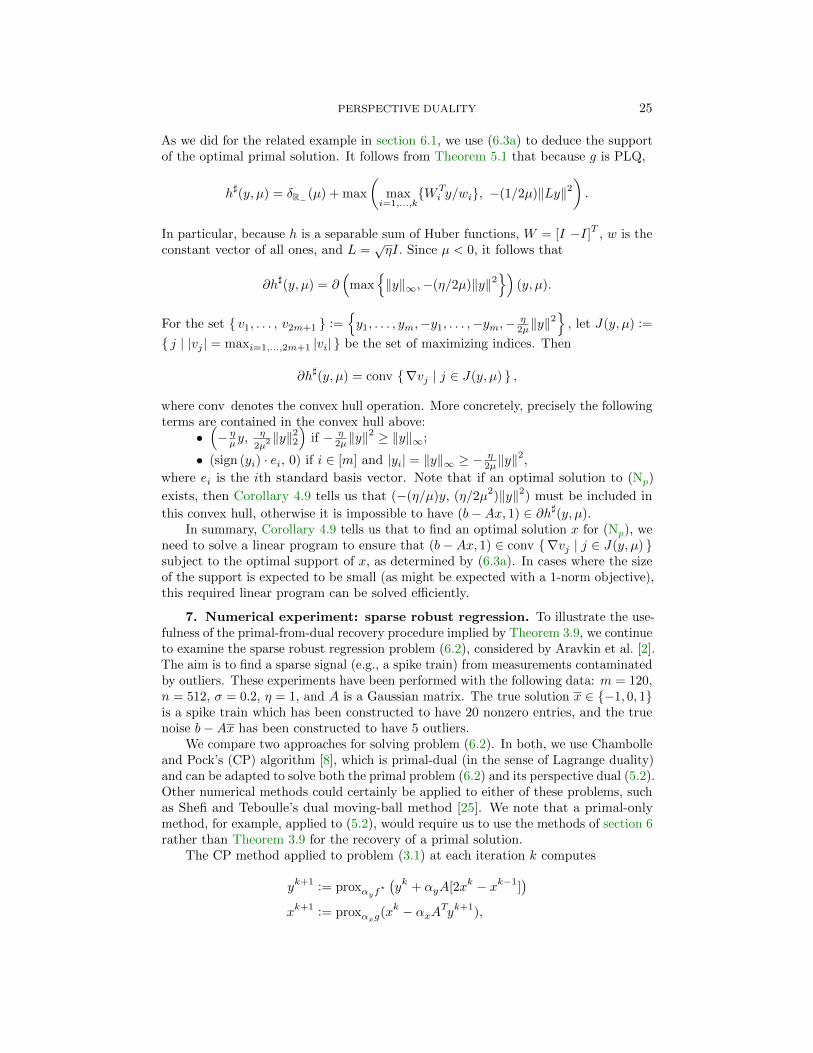
7. Numerical experiment: sparse robust regression. To illustrate the use-fulness of the primal-from-dual recovery procedure implied by Theorem 3.9, we continueto examine the sparse robust regression problem (6.2), considered by Aravkin et al. [2].The aim is to find a sparse signal (e.g., a spike train) from measurements contaminatedby outliers. These experiments have been performed with the following data: m = 120,n = 512, σ = 0.2, η = 1, and A is a Gaussian matrix. The true solution x ∈ {−1, 0, 1}is a spike train which has been constructed to have 20 nonzero entries, and the truenoise b−Ax has been constructed to have 5 outliers.

We compare two approaches for solving problem (6.2). In both, we use Chambolleand Pock’s (CP) algorithm [8], which is primal-dual (in the sense of Lagrange duality)and can be adapted to solve both the primal problem (6.2) and its perspective dual (5.2).Other numerical methods could certainly be applied to either of these problems, suchas Shefi and Teboulle’s dual moving-ball method [25]. We note that a primal-onlymethod, for example, applied to (5.2), would require us to use the methods of section 6rather than Theorem 3.9 for the recovery of a primal solution.

The CP method applied to problem (3.1) at each iteration k computes

yk+1 := proxαyf?

(yk + αyA[2xk − xk−1]

)xk+1 := proxαxg(x

k − αxATyk+1),


200 400 600

iteration

-0.50

-0.25

0.00

0.25

0.50

(obje

ctiv

e -

opti

mum

)/opti

mum

primal

persp. dual

200 400 600

iteration

0

1

2

3

4

5

num

ber

of

fals

e z

ero

s

primal

persp. dual

(a) Normalized objective values (c) False zeros in iterates

200 400 600

iteration

10−3

10−2

10−1

100

101

102

103

feasi

bili

ty v

iola

tion

primal

persp. dual

200 400 600

iteration

0

50

100

150

num

ber

of

fals

e n

onze

ros

primal

persp. dual

(b) Feasibility violations for iterates (d) False nonzeros in iterates

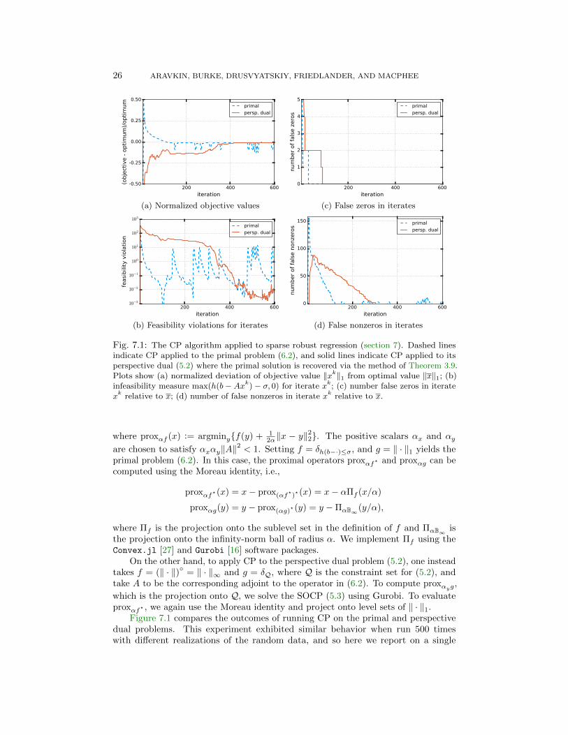
Fig. 7.1: The CP algorithm applied to sparse robust regression (section 7). Dashed linesindicate CP applied to the primal problem (6.2), and solid lines indicate CP applied to itsperspective dual (5.2) where the primal solution is recovered via the method of Theorem 3.9.Plots show (a) normalized deviation of objective value ‖xk‖1 from optimal value ‖x‖1; (b)infeasibility measure max(h(b−Axk)− σ, 0) for iterate xk; (c) number false zeros in iteratexkrelative to x; (d) number of false nonzeros in iterate x

krelative to x.

where proxαf (x) := argminy{f(y) + 12α‖x − y‖

22}. The positive scalars αx and αy

are chosen to satisfy αxαy‖A‖2 < 1. Setting f = δh(b−·)≤σ, and g = ‖ · ‖1 yields the

primal problem (6.2). In this case, the proximal operators proxαf? and proxαg can becomputed using the Moreau identity, i.e.,

proxαf?(x) = x− prox(αf?)?(x) = x− αΠf (x/α)

proxαg(y) = y − prox(αg)?(y) = y −ΠαB∞(y/α),

where Πf is the projection onto the sublevel set in the definition of f and ΠαB∞ isthe projection onto the infinity-norm ball of radius α. We implement Πf using theConvex.jl [27] and Gurobi [16] software packages.

On the other hand, to apply CP to the perspective dual problem (5.2), one insteadtakes f = (‖ · ‖)◦ = ‖ · ‖∞ and g = δQ, where Q is the constraint set for (5.2), andtake A to be the corresponding adjoint to the operator in (6.2). To compute proxαyg,

which is the projection onto Q, we solve the SOCP (5.3) using Gurobi. To evaluateproxαf? , we again use the Moreau identity and project onto level sets of ‖ · ‖1.

Figure 7.1 compares the outcomes of running CP on the primal and perspectivedual problems. This experiment exhibited similar behavior when run 500 timeswith different realizations of the random data, and so here we report on a single


problem instance. Note that performing an iteration of CP on the perspective dualis significantly faster than performing an iteration of CP on the primal because ΠQcan be computed much more efficiently than Πf (see the discussion in section 5.1).This also appears to make convergence of CP on the perspective dual more stable,as seen in Figure 7.1(a). Figure 7.1(c)-(d) illustrate the sparsity patterns of theiterates xk relative to those x. Notably, we recover the correct sparsity patterns usingTheorem 3.9. The recovery procedure outlined in section 6.2 also recovers the correctsparsity pattern, when applied to the final perspective dual iterate.

8. Discussion. Gauge duality is fascinating in part because it shares manysymmetric properties with Lagrange duality, and yet Freund’s 1987 development ofthe concept flows from an entirely different principle based on polarity of the setsthat define the gauge functions. On the other hand, Lagrange duality proceeds from aperturbation argument, which yields as one of its hallmarks a sensitivity interpretationof the dual variables. The discussion in section 3 reveals that both duality notionscan be derived from the same Fenchel-Rockafellar perturbation framework. Thederivation of gauge duality using this framework appears to be its first application toa perturbation that does not lead to Lagrange duality. This new link between gaugeduality and the perturbation framework establishes a sensitivity interpretation forgauge dual variables, which has not been available until now.

One motivation for this work is to explore alternative formulations of optimizationproblems that might be computationally advantageous for certain problem classes. Thephase-retrieval problem, based on an SDP formulation, was a first application of ideasfrom gauge duality for developing large-scale solvers [14]. That approach, however,was limited in its flexibility because it required gauge functions. The discussions ofsection 4 pave the way to new extensions, such as different models of the measurementprocess, as described in section 5.2.

Another implication of this work is that it establishes the foundation for exploring anew breed of primal-dual algorithms based on perspective duality. Our own applicationof Chambolle and Pock’s primal-dual algorithm [8] to the perspective-dual problem,together with a procedure for extracting a primal estimate, is a first exploratory steptowards developing variations of such methods. Future directions of research includethe development of such algorithms, along with their attendant convergence propertiesand an understanding of the classes of problems for which they are practicable.

Acknowledgments. We are grateful to Patrick Combettes for pointing us torecent comprehensive work on properties of the perspective function and its applications[9, 10]. Our sincere thanks to two anonymous referees who provided an extensive listof corrections and suggestions that helped us to arrive at several strengthened resultsand to streamline our presentation.

REFERENCES

[1] A. Y. Aravkin, J. V. Burke, D. Drusvyatskiy, M. P. Friedlander, and S. Roy. Level-set methodsfor convex optimization. arXiv:1602.01506, 2016.

[2] A. Y. Aravkin, J. V. Burke, and M. P. Friedlander. Variational properties of value functions.SIAM J. Optim., 23(3):1689–1717, 2013.

[3] A. Y. Aravkin, J. V. Burke, and G. Pillonetto. Linear system identification using stable splinekernels and PLQ penalties. In 52nd IEEE Decis. Contr. P., pages 5168–5173, Dec 2013.

[4] A. Banerjee, S. Merugu, I. S. Dhillon, and J. Ghosh. Clustering with Bregman divergences. J.Mach. Learn. Res., 6(Oct):1705–1749, 2005.

[5] S. Boyd and L. Vandenberghe. Convex Optimization. Cambridge University Press, 2004.


[6] E. J. Candes, J. Romberg, and T. Tao. Robust uncertainty principles: exact signal reconstructionfrom highly incomplete frequency information. IEEE Trans. Inform. Theory, 52(2):489–509,Feb 2006.

[7] E. J. Candes, J. K. Romberg, and T. Tao. Stable signal recovery from incomplete and inaccuratemeasurements. Comm. Pure Appl. Math., 59(8):1207–1223, 2006.

[8] A. Chambolle and T. Pock. A first-order primal-dual algorithm for convex problems withapplications to imaging. J. Math. Imaging. Vis., 40(1):120–145, 2011.

[9] P. L. Combettes. Perspective functions: Properties, constructions, and examples. Set-ValuedVar. Anal., pages 1–18, 2017.

[10] P. L. Combettes and C. L. Muler. Perspective functions: Proximal calculus and applications inhigh-dimensional statistics. J. Math. Anal. Appl., 2016.

[11] D. Donoho. Compressed sensing. IEEE Trans. Inform. Theory, 52(4):1289–1306, 2006.[12] D. Drusvyatskiy, A. Ioffe, and A. Lewis. Clarke subgradients of directionally Lipschitzian

stratifiable functions. Math. Oper. Res., 40(2):328–349, 2015.[13] R. M. Freund. Dual gauge programs, with applications to quadratic programming and the

minimum-norm problem. Math. Program., 38(1):47–67, 1987.[14] M. P. Friedlander and I. Macedo. Low-rank spectral optimization via gauge duality. SIAM J.

Sci. Comput., 28(3):A1616–A1638, 2016.[15] M. P. Friedlander, I. Macedo, and T. K. Pong. Gauge optimization and duality. SIAM J.

Optim., 24(4):1999–2022, 2014.[16] I. Gurobi Optimization. Gurobi optimizer reference manual, 2015.[17] P. Huber. Robust Statistics. Wiley, 1981.[18] J. A. Nelder and R. J. Baker. Generalized linear models. Encyclopedia of statistical sciences,

1972.[19] Y. Nesterov and A. Nemirovskii. Interior-point polynomial algorithms in convex programming,

volume 13. SIAM, 1994.[20] R. T. Rockafellar. Convex Analysis. Princeton University Press, 1972.[21] R. T. Rockafellar. Conjugate duality and optimization. SIAM, 1974.[22] R. T. Rockafellar. First- and second-order epi-differentiability in nonlinear programming. Trans.

Amer. Math. Soc., 307(1):75–108, May 1988.[23] R. T. Rockafellar and R. J.-B. Wets. Variational Analysis, volume 317. Springer Science &

Business Media, 2009.[24] R. Shefi and M. Teboulle. A dual method for minimizing a nonsmooth objective over one

smooth inequality constraint. Math. Program., 159(1-2):137–164, 2016.[25] R. Shefi and M. Teboulle. On the rate of convergence of the proximal alternating linearized

minimization algorithm for convex problems. EURO J. Comp. Optim., 4(1):27–46, 2016.[26] J. Tropp. Just relax: convex programming methods for identifying sparse signals in noise. IEEE

Trans. Inform. Theory, 52(3):1030–1051, 2006.[27] M. Udell, K. Mohan, D. Zeng, J. Hong, S. Diamond, and S. Boyd. Convex optimization in Julia.

SC14 Workshop on High Performance Technical Computing in Dynamic Languages, 2014.[28] H. Zou and T. Hastie. Regularization and variable selection via the elastic net. J. R. Stat. Soc.

Ser. B Stat. Methodol., 67(2):301–320, 2005.

Appendix A. Proof of (2.6). We prove each fact in succession.1. (U◦κ = Uκ◦). By definition of the polar gauge and the polar cone, we havey ∈ Uκ◦ if and only if

sup { 〈x, y〉 | κ(x) ≤ 1 } ≤ 1 ⇐⇒ y ∈ U◦κ .

2. (U∞κ = Hκ). Suppose x ∈ Hκ. Then for any u ∈ Uκ and λ > 0, by sublinearityof κ we have κ(u+λx) ≤ κ(u)+λκ(x) ≤ 1+λ ·0 = 1. Thus x ∈ U∞κ , and Hκ ⊆U∞κ . Suppose now that y ∈ U∞κ \Hκ. Then in particular, κ (y/κ(y) + λy) ≤ 1for all λ > 0. But then by positive homogeneity, (1/κ(y) + λ)κ(y) ≤ 1, for allλ > 0. This is a contradiction since κ(y) > 0, so we conclude that Hκ = U∞κ .

3. ((domκ)◦ = Hκ◦). By positive homogeneity of κ and the definition of thepolar gauge, y ∈ Hκ◦ if and only if

supκ(x)≤1

〈x, y〉 = 0 ⇐⇒ supκ(x)<∞

〈x, y〉 = 0 ⇐⇒ y ∈ (domκ)◦.


4. (H◦κ = cl domκ◦). Apply the third equality, replacing κ by κ◦, and then takepolars on both sides. This concludes the proof.

Appendix B. Proof of Lemma 3.3. With no loss in generality, we can assumethat σ > 0, because if σ = 0, we use the convention (2.8) and its implication (2.9).

First suppose that the primal (Gp) is relatively strictly feasible. A point u lies inthe domain of p if and only if the system

(u, 0, 0) ∈M[wλ

]+ (epi ρ)× Uκ, where M :=

[A −b0 −σ−I 0

],

is solvable for (w, λ). Thus the set (dom p)× {0} × {0} coincides with

(B.1) L⋂

(rangeM + (epi ρ)× Uκ) ,

where L := { (a, b, c) | b = 0, c = 0 } is a linear subspace. We aim to show (0, 0, 0) isin the relative interior of (B.1), which will show 0 ∈ ri dom p. Use [20, Lemma 7.3]and [20, Theorem 7.6] to obtain

ri epi ρ = { (z, r) ∈ (ri dom ρ)× R | ρ(z) < r }riUκ = {x ∈ ri domκ | κ(x) < 1 } .

From relative strict feasibility of (Gp), the fact that σ > 0, and again [20, Theorem7.6], we deduce existence of an x ∈ ri domκ with b−Ax ∈ ri dom ρ and ρ(b−Ax) < σ.Fix a constant r > κ(x) and define the pair (w, λ) := (x/r, 1/r). Then we immediatelyhave (bλ−Aw, σλ) ∈ ri epi ρ and κ(w) < 1. It follows that the vector −M [wλ ] lies in(ri epi ρ)× riUκ. Thus (0, 0, 0) lies in the intersection

(B.2) L⋂

(rangeM + [(ri epi ρ)× riUκ]) .

Use [20, Theorem 6.5, Corollary 6.6.2] to deduce that (B.2) is the relative interior ofthe intersection (B.1). Thus y = 0 lies in the relative interior of dom p as claimed.

Next, suppose that the gauge dual (Gd) is strictly feasible. By definition of F ?,the tuple (w, λ) lies in the domain of vd if and only if

(w, 0,−λ) ∈(domκ◦ × epi(σρ◦ − 〈b, ·〉+ 1)

)− rangeB, with B :=

[AT

I0

].

Thus dom vd is linearly isomorphic to the intersection

(B.3) L′⋂((

domκ◦ × epi(σρ◦ − 〈b, ·〉+ 1))− rangeB

),

where L′ is the linear subspace L′ := {(a, b, c) | b = 0}. However, by [20, Lemma 7.3],relative strict feasibility of the dual (Gd) amounts to the inclusion

(0, 0, 0) ∈(ri domκ◦ × ri epi(σρ◦ − 〈b, ·〉+ 1)

)− rangeB.

Strict feasibility of (Gd) implies, via [20, Corollary 6.5.1, Corollary 6.6.2], that (0, 0, 0)is in the relative interior of the intersection (B.3), and thus 0 ∈ ri dom vd, as claimed.

Finally, the exact same arguments, but with relative interiors replaced by interiors,will prove the claims relating strict feasibility and interiority. This concludes the proof.

FOUNDATIONS OF GAUGE AND PERSPECTIVE DUALITYmpf/pdfs/2017PerspectiveDuality.pdf · FOUNDATIONS OF...

Documents

Transcript of FOUNDATIONS OF GAUGE AND PERSPECTIVE DUALITYmpf/pdfs/2017PerspectiveDuality.pdf · FOUNDATIONS OF...