Forward-looking Risk Measurement - Moody's Analytics

May 2021

Armen Mirzoyan, Associate Director, MA Predictive Analytics Unit

Gega Todua, Assistant Director, MA Predictive Analytics Unit

Forward-looking Risk MeasurementA Moody’s Analytics Presentation

Forward-Looking Risk 2

1 Overview


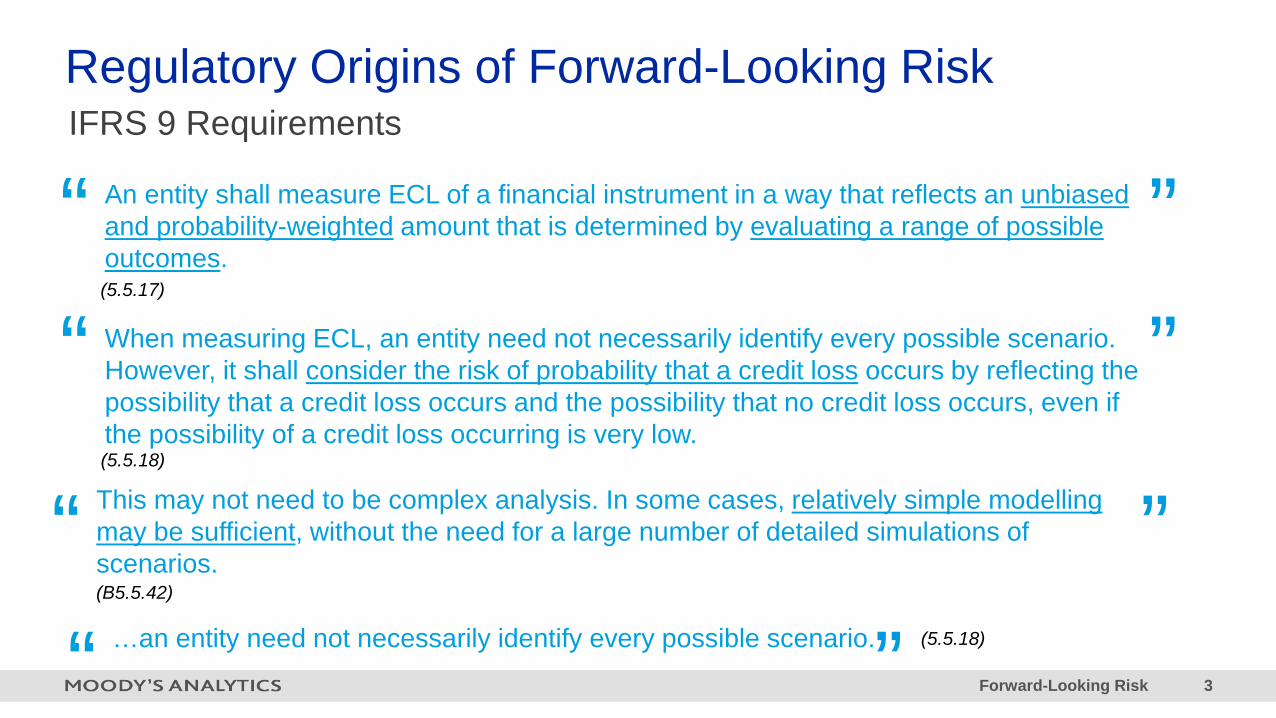
IFRS 9 Requirements

(5.5.17)

An entity shall measure ECL of a financial instrument in a way that reflects an unbiased and probability-weighted amount that is determined by evaluating a range of possible outcomes.

“ ”

(5.5.18)

When measuring ECL, an entity need not necessarily identify every possible scenario. However, it shall consider the risk of probability that a credit loss occurs by reflecting the possibility that a credit loss occurs and the possibility that no credit loss occurs, even if the possibility of a credit loss occurring is very low.

“ ”This may not need to be complex analysis. In some cases, relatively simple modelling may be sufficient, without the need for a large number of detailed simulations of scenarios.“ ”(B5.5.42)

…an entity need not necessarily identify every possible scenario.“ ” (5.5.18)

Regulatory Origins of Forward-Looking Risk


Forward Looking & Probability-Weighted Outcomes

» Requires expected credit losses (ECL) to account for forward-looking information

» Requires probability-weighted outcomes when measuring expected credit losses – Estimates should reflect the possibility that a credit loss occurs and the possibility that no credit loss occurs

Macroeconomic modelling satisfies both requirements above

Key Take-Aways


2 Macroeconomic Forecasting


2.1 Coverage and Key Features


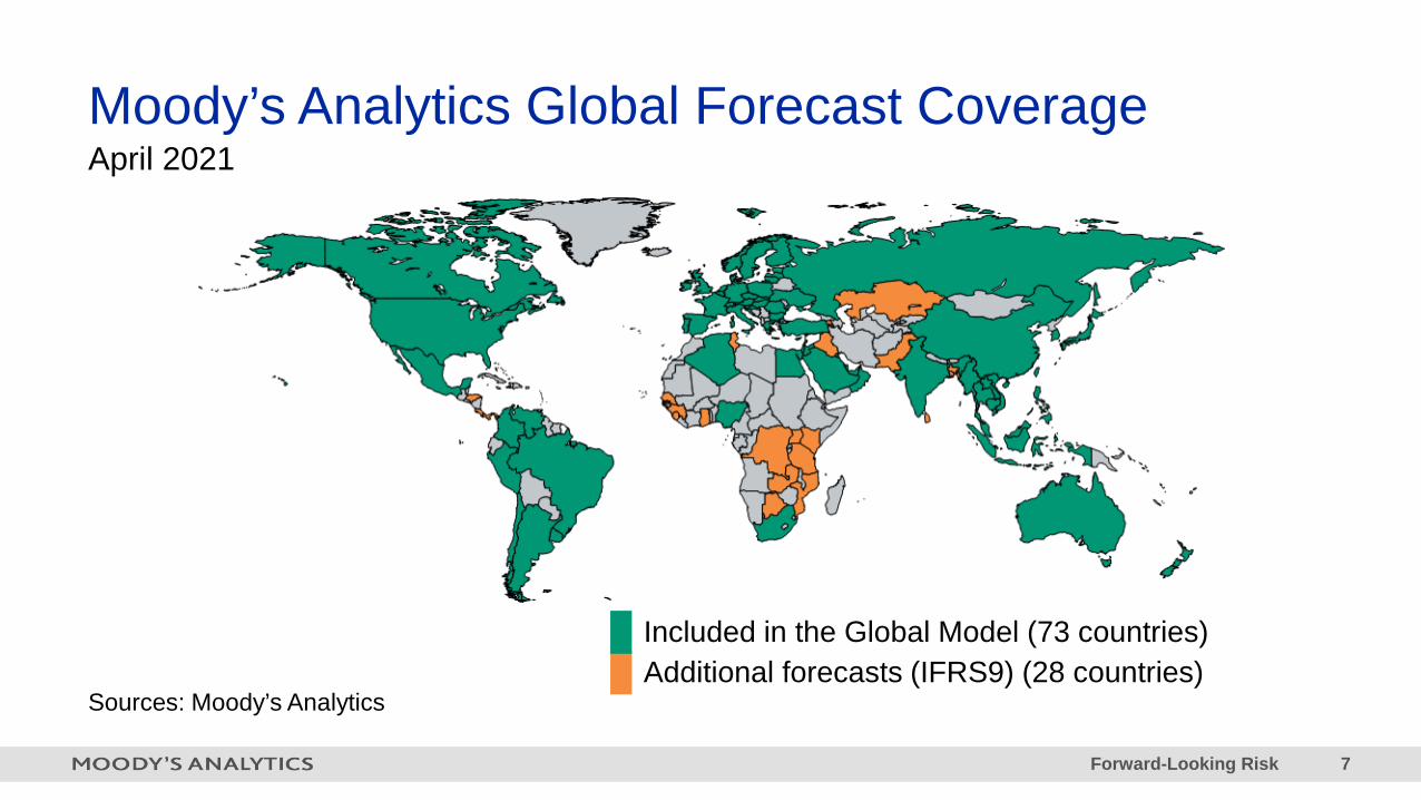
Moody’s Analytics Global Forecast CoverageApril 2021

Sources: Moody’s Analytics

Included in the Global Model (73 countries)Additional forecasts (IFRS9) (28 countries)


Key Features

Collaborative Access and Integration Develop scenarios individually or collaboratively in a real-time, multi-user environment.

Integrate forecasts into your workflow seamlessly through our API and Excel Add-In.

Comprehensive CoverageCreate scenarios for 101 countries and 10 regional aggregates, out to 30-years.

Evaluate monthly updated forecasts for 10,000+ economic and financial time series.

Robust Editing & Visualization ToolsAdjust detailed variables to simulate shocks or more discrete factors.

Visualize your changes through interactive dashboards, charting and data tables.


2.2 Moody’s Global Macroeconomic Model


Linkages in the model allow for global shock propagation and contagion effects, and help ensure scenario consistency

» Trade flows (exports reflect partner imports)

» Financial markets (stock prices and bond yields)

» Prices (exchange rates, terms of trade and global commodity prices)

» Investment (foreign direct investment and capital flows)

Diagnostic processes ensure that our forecasts are stable from month to month and consistent withthe business cycle outlook of each nation.

Provides Globally Linked ForecastsGlobal Macroeconomic Model


Each Country-model is a Mix of Theory and Data

Modelling Approach

Our ModelsIntersection of purely data- and

purely theory-based models

Theory» Quality of forecast and scenarios » Complex» Limited quantity of forecasts

Data» Quality and quantity of forecasts» Easy to produce» Not ideal for scenario analysis


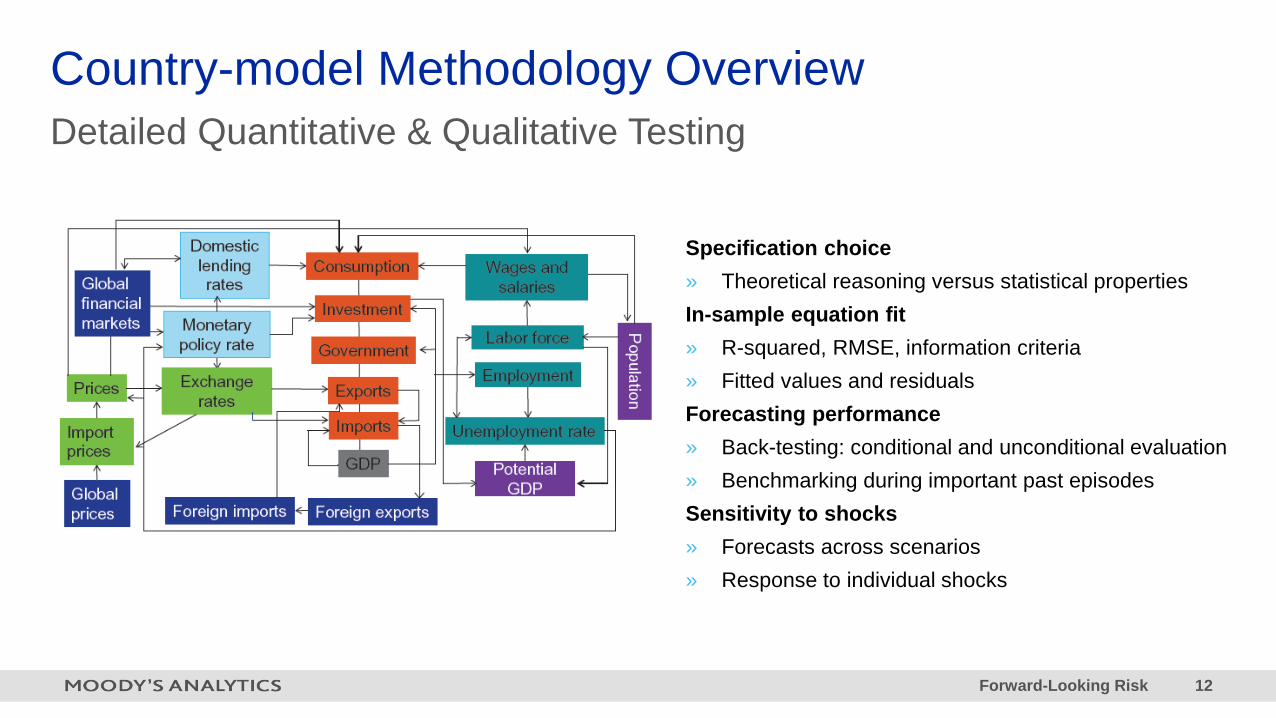
Detailed Quantitative & Qualitative TestingCountry-model Methodology Overview

Specification choice» Theoretical reasoning versus statistical propertiesIn-sample equation fit» R-squared, RMSE, information criteria» Fitted values and residualsForecasting performance» Back-testing: conditional and unconditional evaluation» Benchmarking during important past episodesSensitivity to shocks» Forecasts across scenarios» Response to individual shocks

13

Identify Equation for Development•Revised indicator•New indicator•Indicator with poor performance

•Model owners prioritize based on need, use, and performance

Equation Estimation•Specification•Variable selection•In-sample fit•Out-of-time fit•Theoretical consistency

Model Integration Testing•Test inclusion of proposed equation in model system

•Examine impact on other core indicators

•Examine shock properties

Equation Approval•Model owner examines equation development results and impact analysis

•Model validator examines test results

•Joint approval required to advance proposed equation

Equation Implementation•Production team implements equation specs

•Runs battery of stability tests. •Generates baseline forecast output

•Model owner confirms forecast output as intended

Documentation•Equation estimation codes, results, summary findings archived

•Production equations published to user interfaces

•Model system documentation refreshed annually

Validation•Independent validation team

•Reviews key equations•Reviews overall model system performance

•Performs historical backtesting

•Identifies issues•Recommends

Production Release•Equation integrated into monthly forecasting process

•Forecasts reviewed and adjusted per forecast governance procedures

Performance Tracking•Monthly performance tracking report

•Compares forecasted versus actual performance

•Considers several model vintages

•Published to users

Performance Review•Analyst examines performance monthly

•Flags indicators for watchlist

•Escalates indicators with poor performance to model owners

Rigorous Equation Development Process


Equations Designed to Balance Theory & EmpiricsVariable Specification suggested by economic theory draws on…Unemployment rate Okun's LawLabor Force Participation rate & demographicsPrivate consumption expenditure Keynesian consumption function / Euler equationPublic consumption expenditure Baumol's disease w/ endogenous responses to fiscal spaceFixed investment Accelerator model / Tobin's QInventory investment Adjustment process in deviations of final spending to firm outputExports Trading partner import demand and real effective exchange rateImports Imports reflect domestic demand + re-exporting demandLabor income (wages & salaries) Wage bargaining over revenue product of laborCentral bank target rate Policy assumption, based on an augmented Taylor Rule10yr Gov bond yield Fisher Rule w/ sovereign risk premium, global interest rate parityYield curve & market lending rates Term-structure of interest ratesExchange rate (floating) Interest rate parity (short-run) & purchasing power parity (long-run)Import price deflator Exchange rate pass-through of foreign prices, global commodity pricesConsumer price index Expectations augmented Phillip's curve based on firm price setting functionHouse prices, stock prices Asset pricing theoryGovernment total expenditure Sum of government consumption + debt service + net transfersGovernment total revenues Revenues equal the effective tax rate multiplied by incomeIndustrial production IP tracks the aggregate value added of goods-producing industriesDomestic credit (money supply) Liquidity demand depends on transactions value (GDP) and interest ratesCA balance (Identity) CA = net exports + net income + net transfers


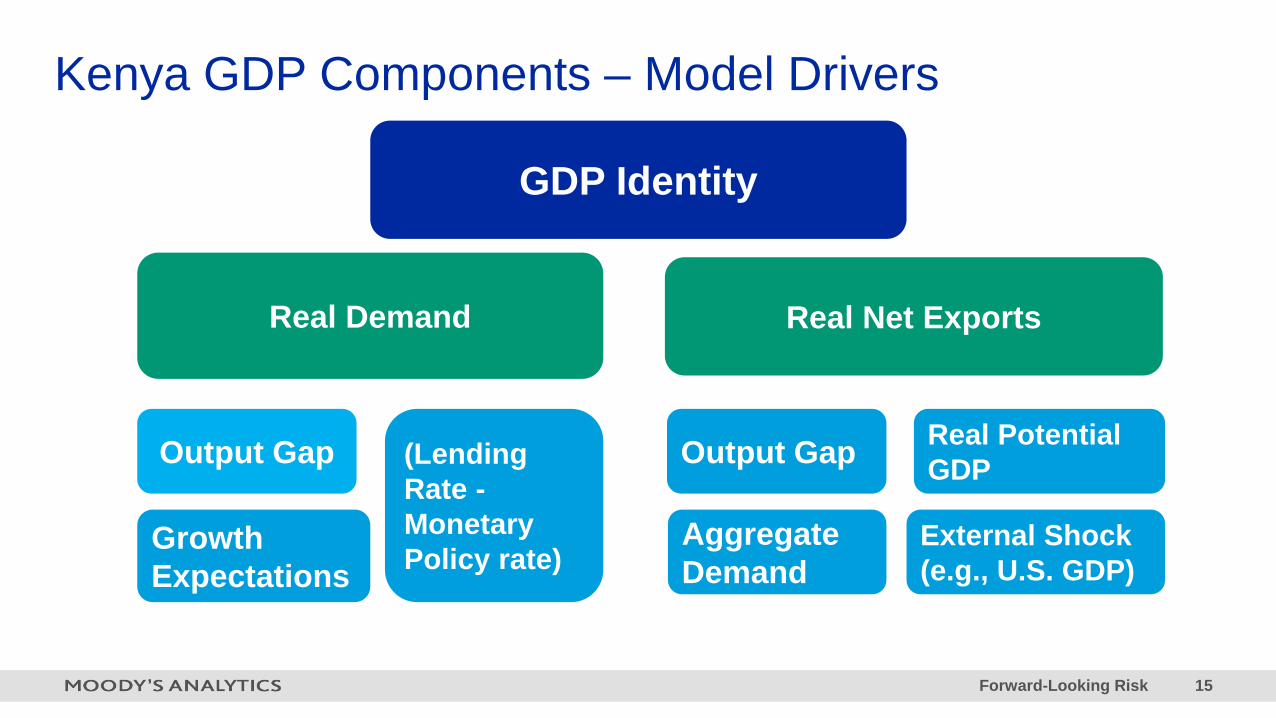
Kenya GDP Components – Model Drivers

Output Gap

Growth Expectations

Real Demand

GDP Identity

(Lending Rate -Monetary Policy rate)

Real Net Exports

Output Gap Real Potential GDP

Aggregate Demand

External Shock (e.g., U.S. GDP)


Baseline Forecasting

Sources: ECB, Moody’s Analytics

-10.0

-5.0

0.0

5.0

10.0

15.0

2007Q1 2012Q1 2017Q1 2022Q1 2028Q2 2033Q2

US

-9.0

-4.0

1.0

6.0

11.0

16.0

21.0

2007Q1 2012Q1 2017Q1 2022Q1 2027Q1 2032Q1

China

-15.0

-10.0

-5.0

0.0

5.0

10.0

15.0

2007Q1 2012Q1 2017Q1 2022Q1 2027Q1 2032Q1

Eurozone

-6.0

-1.0

4.0

9.0

14.0

2007Q1 2012Q1 2017Q1 2022Q1 2027Q1 2032Q1

Kenya

Real GDP, % chg year ago Real GDP, % chg year ago

Real GDP, % chg year agoReal GDP, % chg year ago


2.3 Scenario Generation


Phases of Scenario Workflow

Key Assumptionsx

Global Macroeconomic

Modely

Market and Credit Risk Models

z(x,y)

Combined Forecast

(x,y,z)

Credit risk (PD, LGD, EAD, ECL) and market risk instruments forecast

Macroeconomic series forecast


Standard Scenarios

Moody’s Analytics Off-the-Shelf Scenarios

Expanded Regulatory Scenarios

Custom Scenarios

Partially or Fully Specified Economy Assumptions

Thematic Event-Driven Scenarios

Scenario Studio

Web-based Scenario Building Application

Real-time Rigorous Forecasting Process

Forecasts for 70+ countries used by 780 Clients worldwide

Scenario Generation Using Moody’s Analytics Global Model

S1 S2 S3 S4BL S5 S6 S8 FED PRA EBA CU

MOODYS’ ANALYTICS BASELINE + S1-S8 , S0 EXPANDED REGULATORY CUSTOM

S0 CO

CONSENSUS


Pillars of Scenario Generation

ISeverity

Quantitative representation of “How favorable/adverse is given scenario”

Ensures that scenarios are representative and symmetric

around baselineGuides assignment of probability

weights

IINarrative

Determines overall nature of the scenario and guides the exact path

of forecastsHelps with understanding and

interpretation of scenariosEnsures that scenarios are globally

consistent

IIITransmission

Global linkages in models transmit shocks across countries

Ensures consistency of forecasts across countries

Delivers sizable initial shocks to models


GDP Growth %, Annualized avg., 10,000 Simulations over a 5-yr PeriodScenario Calibration: Discrete Scenario Prob.

Source: Moody’s Analytics

0

100

200

300

400

500

600

700

800

-2.6 -1.8 -1.0 -0.2 0.6 1.4 2.2 3.0 3.8 4.6 5.4

S0: 96%severity

S0: 7% WeightS3: 10% downside severity

S3: 23% WeightBL

0.50 Severity40% Weight S1: 23% Weight

S1: 90% severity

S4: 4% downside severity

S4: 7% Weight


Scenario Forecasting

15,000

17,000

19,000

21,000

23,000

18 19F 20 21F 22F 23F 24F 25F 26F 27F 28F

S1

S3

Baseline

78,00088,00098,000

108,000118,000128,000138,000148,000

18 19F 20 21F 22F 23F 24F 25F 26F 27F 28F

S1

S3

Baseline

9,0009,500

10,00010,50011,00011,50012,00012,500

18 19F 20 21F 22F 23F 24F 25F 26F 27F 28F

S1

S3

Baseline

4,500

5,000

5,500

6,000

6,500

7,000

7,500

8,000

18 19F 20 21F 22F 23F 24F 25F 26F 27F 28F

S1

S3

Baseline

U.S. GDP, 2012 bil. USD China GDP, 2015 Bil. CNY

Kenya GDP, 2009 Bil. KESEuro Zone Inflation, % change yr ago

Sources: Eurostat, ECB, Moody’s Analytics


2.4 Scenario Studio


High-quality data

Sound model

Sound assumpt-

ionsLogistics

Comprising:» Process – The steps

taken in the production of a forecast

» Platform – the tools used to implement the forecasting process

Specifically:» Up-to-date» No errors» Long time series» Temporally consistent» Accurately calculated

Elements of Forecast Integrity


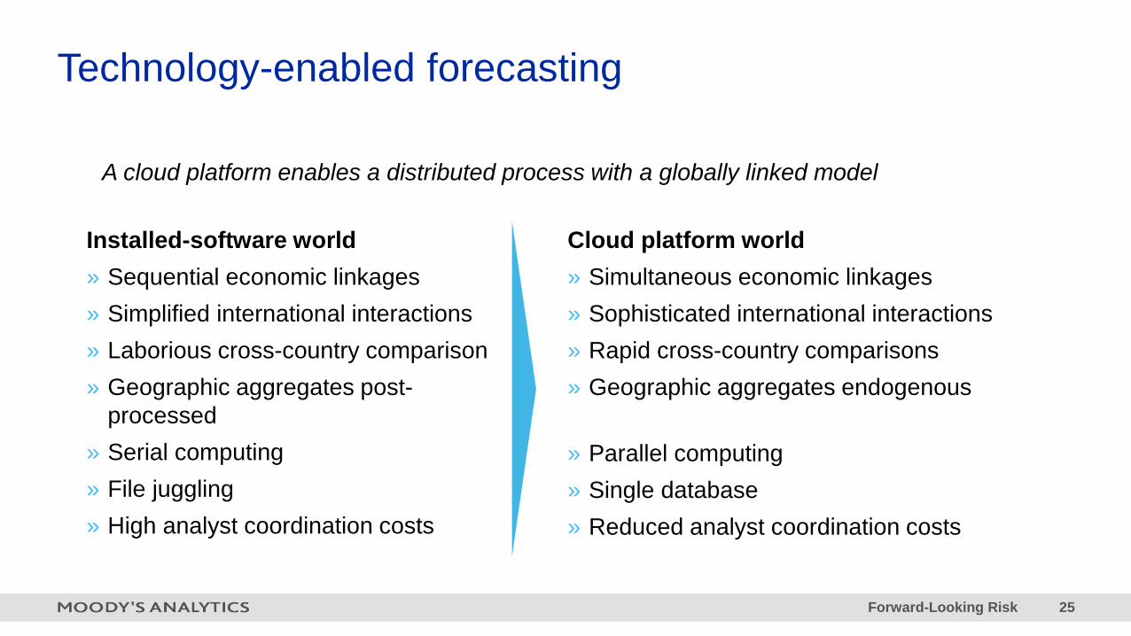
Installed-software world» Sequential economic linkages» Simplified international interactions» Laborious cross-country comparison» Geographic aggregates post-

processed» Serial computing» File juggling» High analyst coordination costs

Cloud platform world» Simultaneous economic linkages» Sophisticated international interactions» Rapid cross-country comparisons» Geographic aggregates endogenous

» Parallel computing» Single database» Reduced analyst coordination costs

A cloud platform enables a distributed process with a globally linked model

Technology-enabled forecasting


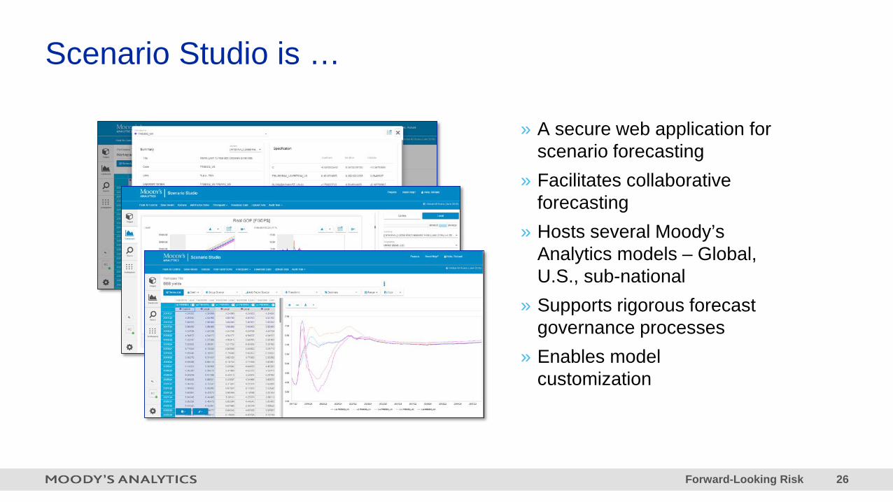
» A secure web application for scenario forecasting

» Facilitates collaborative forecasting

» Hosts several Moody’s Analytics models – Global, U.S., sub-national

» Supports rigorous forecast governance processes

» Enables model customization

Scenario Studio is …


3 Forward-looking Risk


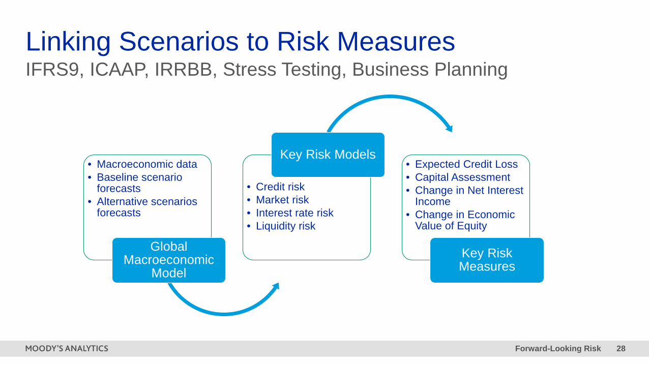
Linking Scenarios to Risk Measures

• Macroeconomic data• Baseline scenario

forecasts• Alternative scenarios

forecasts

Global Macroeconomic

Model

• Credit risk• Market risk• Interest rate risk• Liquidity risk

Key Risk Models• Expected Credit Loss• Capital Assessment• Change in Net Interest

Income• Change in Economic

Value of Equity

Key Risk Measures

IFRS9, ICAAP, IRRBB, Stress Testing, Business Planning


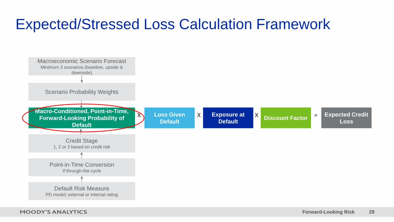
Expected/Stressed Loss Calculation Framework

Macroeconomic Scenario ForecastMinimum 3 scenarios (baseline, upside &

downside)

Scenario Probability Weights

Macro-Conditioned, Point-in-Time, Forward-Looking Probability of

Default

Credit Stage1, 2 or 3 based on credit risk

Point-in-Time ConversionIf through-the-cycle

Default Risk MeasurePD model; external or internal rating

Loss Given Default

Exposure at Default Discount Factor Expected Credit

LossX X X =


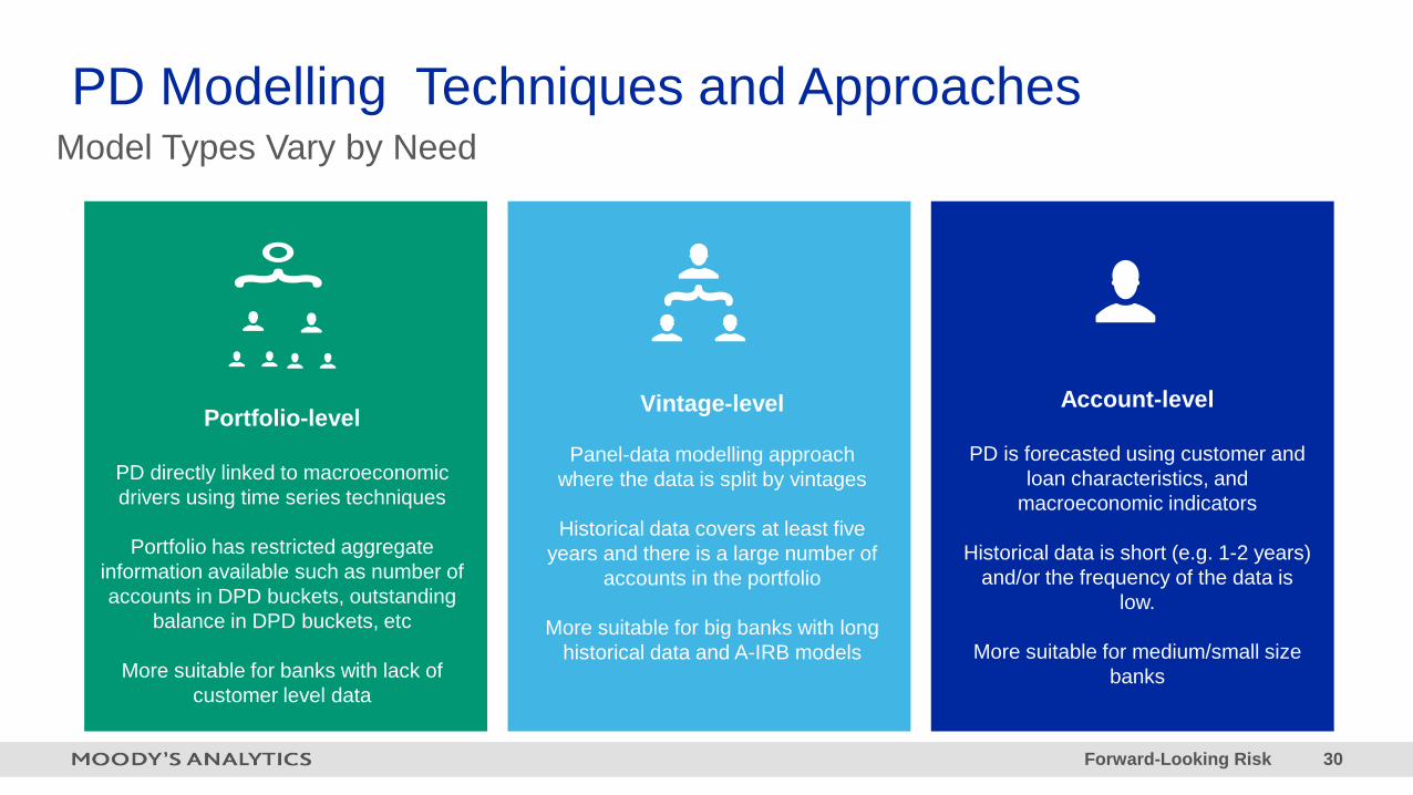
PD Modelling Techniques and ApproachesModel Types Vary by Need

Vintage-level

Panel-data modelling approach where the data is split by vintages

Historical data covers at least five years and there is a large number of

accounts in the portfolio

More suitable for big banks with long historical data and A-IRB models

Account-level

PD is forecasted using customer and loan characteristics, and

macroeconomic indicators

Historical data is short (e.g. 1-2 years) and/or the frequency of the data is

low.

More suitable for medium/small size banks

Portfolio-level

PD directly linked to macroeconomic drivers using time series techniques

Portfolio has restricted aggregate information available such as number of accounts in DPD buckets, outstanding

balance in DPD buckets, etc

More suitable for banks with lack of customer level data


PD Vintage-level Approach

Variable capturing the heterogeneity across cohorts: vintage dummies,

portfolio characteristics (LTV, asset class/collateral type, geography, etc.)

and/or economic conditions at origination

Lifecycle Quality of Vintage Forward-looking Indicator

Dynamic evolution of vintages as they mature

Sensitivity of performance to the evolution of macroeconomic and credit

series

PD= f( , , )

00.010.020.030.040.050.060.070.080.090.1

1 2 3 4 5 6 7 8 9 10 11 12 13 14 15 16

PD

Age

0

0.02

0.04

0.06

0.08

0.1

0.12

0.14

0.16

1 2 3 4 5 6 7 8 9 10 11 12 13 14 15 16

PD

Age

00.010.020.030.040.050.060.070.080.090.1

t0 t+4 t+8 t+12 t+16 T

PD

Time


PD Vintage-level ApproachMortgages Example

Vintage dummies

Economic conditions at origination

Portfolio data at origination

1. Lifecycle 2. Quality of Vintage 3. Forward-looking Indicator

Large number of accounts leads to implementation problems.

Solution:Build curves based on the different combinations of score bins, segments and vintages.

Final PD Model

0

0.002

0.004

0.006

0.008

0.01

0.012

0.014

0.016

0.018

0.02

1 11 21 31 41 51 61 71 81

PD

Age

Predicted Lifecycle

Lifecycle

0.000

0.005

0.010

0.015

0.020

0.025

0.030

0.035

1 11 21 31

PD

Age

-0.15

-0.1

-0.05

0

0.05

0.1

0.15

T-k T-30 T-15 T T+15 T+30 T+45 T+60 T+75 T+m

PD

Time

HPI YoY GrowthHistory Baseline Upside Downside

0

0.005

0.01

0.015

0.02

0.025

T-k T-4 T T+4 T+m

PD

Time

Default Rate Fitted Values BaselineFitted Values Upside Fitted Values Downside


PD Vintage-level ApproachCredit Cards Example

Vintage dummies

Economic conditions at origination

Portfolio data at origination

1. Lifecycle 2. Quality of Vintage 3. Forward-looking Indicator

0

0.002

0.004

0.006

0.008

0.01

0.012

1 5 9 13 17 21 25 29

PD

Age

Predicted Lifecycle

Lifecycle

Large number of accounts leads to implementation problems.

Solution:Build curves based on the different combinations of score bins, segments and vintages.

0

0.002

0.004

0.006

0.008

0.01

0.012

0.014

1 2 3 4 5 6 7 8 9 10 11 12 13 14 15 16

PD

Age

-0.06

-0.04

-0.02

0

0.02

0.04

0.06

0.08

T - k T T+15 T+30

Time

Private Consumption (YoY Growth)History Baseline Upside Downside

Final PD Model

0

0.0005

0.001

0.0015

0.002

0.0025

0.003

T-k T-12 T-9 T-6 T-3 T T+3 T+6 T+9 T+k

PD

Time

Default Rate Fitted Values Baseline

Fitted Values Upside Fitted Values Downside


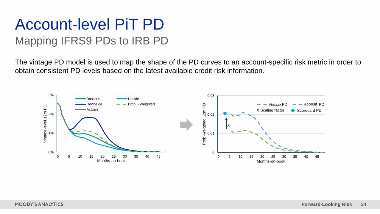
Account-level PiT PDMapping IFRS9 PDs to IRB PD

The vintage PD model is used to map the shape of the PD curves to an account-specific risk metric in order to obtain consistent PD levels based on the latest available credit risk information.

0%

1%

2%

3%

0 5 10 15 20 25 30 35 40 45

Vint

age-

leve

l12m

PD

Months-on-book

Baseline UpsideDownside Prob. - WeightedActuals

0

0.01

0.02

0.03

0 5 10 15 20 25 30 35 40 45

Prob

.-wei

gthe

d12

m P

D

Months-on-book

Vintage Account

K

K Scaling factor Scorecard PDPD PD


Portfolio-level Modelling

» If a portfolio has restricted aggregate information available such as number of accounts in DPD buckets, outstanding balance in DPD buckets, etc.:

– Model default rate calculated as number of defaulted accounts at time t on total number of accounts at time t. Link to macro drivers.

– Alternatively, use another portfolio-related metric as the dependent variable: portfolio delinquency, total balance, portfolio age, etc.

0 – 29 DPD 30-59 DPD 60-89 DPD 90-119 DPD

0-29 DPD 95.37% 2.13% 0.69% 1.81%

30-59 DPD 77.57% 1.82% 0.64% 19.97%

60-89 DPD 43.57% 1.05% 0.38% 55.00%

90-119 DPD 0.00% 0.00% 0.00% 100.00%

0.04

0.06

0.08

0.1

0.12

0.14

0.16

0.18

T-k T-26 T T+26 T+52 T+78 T+m

PD

Time

PD Baseline PD Upside PD Downside


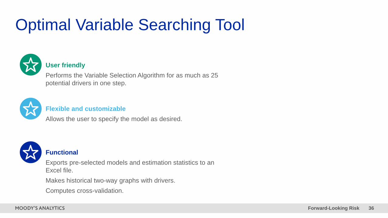
Optimal Variable Searching Tool

User friendlyPerforms the Variable Selection Algorithm for as much as 25 potential drivers in one step.

Flexible and customizableAllows the user to specify the model as desired.

FunctionalExports pre-selected models and estimation statistics to an Excel file.Makes historical two-way graphs with drivers.Computes cross-validation.


OVS Customizable Features

» Target variable

» Scenarios

» Potential drivers and expected signs

» Maximum number of drivers in the final model

» Maximum number of lags for drivers

» Estimator and estimation options: any built-in estimator in the software

» Correlation coefficient threshold. Default value is 0.75.

» Maximum p-value on estimated coefficients. Default is 0.05

» Additional variables that enter in the model by default


Dynamic Credit Risk Model-BuildingVariable selection for scenario-conditional forecasting

All combinations of size k from vector m

𝑪𝑪𝒎𝒎𝒌𝒌

Exclude models with collinear drivers

Pairwise Correlations(optional)

Ranking Criteria• Adjusted R2/RMSE• Likelihood-based criteria• Stationarity and cointegration• Validation

Optimal Model

k: right-hand-side variablesm: potential economic & internal drivers

• Expected estimated signs on drivers • Statistically significant drivers

Selection Criteria(optional)

Best Subset Variable Selection Algorithm


Optimal Variable Searching ToolWeb Application

» Allows to run OVS on your own data

» No R installation needed

» Runs in browser

» Easy-to-use, no code involved

» 3 menu items on the sidebar with the last one showing OVS results

1. File upload

– upload a file with data in CSV format– upload the appropriate permutation

file – supplied by Moody’s


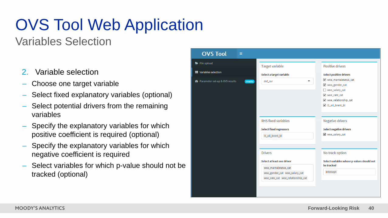
OVS Tool Web ApplicationVariables Selection

2. Variable selection– Choose one target variable– Select fixed explanatory variables (optional)– Select potential drivers from the remaining

variables– Specify the explanatory variables for which

positive coefficient is required (optional)– Specify the explanatory variables for which

negative coefficient is required – Select variables for which p-value should not be

tracked (optional)


OVS Tool Web ApplicationParameter Set-up & Results

3. Parameter set-up & OVS results– Choose the maximum number of drivers that can

be included in the model– Specify a p-value threshold for testing

significance of explanatory variables– Input path to a file where you want to export the

OVS results and a file name– Specify the maximum correlation coefficient

between each pair of variables– Choose GLM type that will be used for estimation– Press the run OVS button to obtain results– Results appear in the table below and they are

exported to the file you specified


Significant Increase in Credit Risk

0.0%

1.0%

2.0%

3.0%

4.0%

5.0%

6.0%

7.0%

0 6 12 18 24 30 36 42 48 54 60 66 72 78 84 90 96 102 108 114 120 126 132 138Age (Months-on-book)

Account-level Reporting Lifetime PD Account-level Origination Lifetime PD

d

d Distance to assess for threshold» To measure the change in risk since initial recognition, we examine the proportional difference between

– the lifetime PD at the reporting date Lifetime PD(T) , and

– the lifetime PD at the same age as the reporting date forecasted at origination Lifetime PD0(T)

» Distance b is utilized as the metric and is the percentage increase to the lifetime PD curve between origination and reporting date. Increases are examined to determine how to identify which are deemed significant.


LGD Design ApproachesBalance and RecoveriesFor a facility i, time t and workout period w:

𝐿𝐿𝐿𝐿𝐿𝐿𝑖𝑖 = 1 −𝑏𝑏𝑏𝑏𝑏𝑏𝑏𝑏𝑏𝑏𝑏𝑏𝑏𝑏𝑖𝑖,𝑡𝑡 − 𝑏𝑏𝑏𝑏𝑏𝑏𝑏𝑏𝑏𝑏𝑏𝑏𝑏𝑏𝑖𝑖,𝑡𝑡+𝑤𝑤

𝑏𝑏𝑏𝑏𝑏𝑏𝑏𝑏𝑏𝑏𝑏𝑏𝑏𝑏𝑖𝑖,𝑡𝑡

By AssumptionLGD of 50-60% for PF, 30-40% for RE and 65-75% for CC; fully insured products usually get LGD of 5-10%.Estimates of recovery costs range from 1-2%.

Default Vintages & Macro Drivers Roll Rate Modelling

𝑅𝑅𝑅𝑅𝑖𝑖𝑡𝑡 = 1 − 𝐿𝐿𝐿𝐿𝐿𝐿𝑖𝑖𝑡𝑡


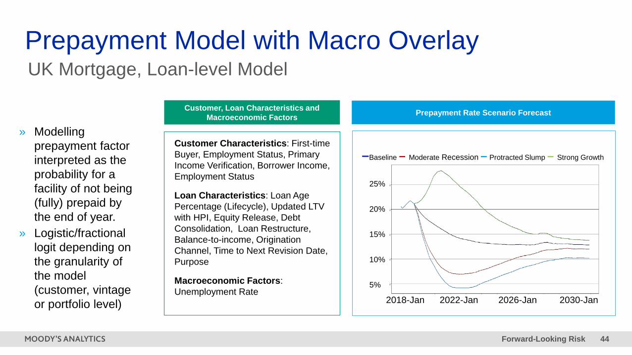
Prepayment Model with Macro Overlay

Customer, Loan Characteristics and Macroeconomic Factors

Customer Characteristics: First-time Buyer, Employment Status, Primary Income Verification, Borrower Income, Employment Status

Loan Characteristics: Loan Age Percentage (Lifecycle), Updated LTV with HPI, Equity Release, Debt Consolidation, Loan Restructure, Balance-to-income, Origination Channel, Time to Next Revision Date, Purpose

Macroeconomic Factors: Unemployment Rate

Prepayment Rate Scenario Forecast

2018-Jan 2022-Jan 2026-Jan 2030-Jan

25%

20%

15%

10%

5%

–Baseline – Moderate Recession – Protracted Slump – Strong Growth

UK Mortgage, Loan-level Model

» Modelling prepayment factor interpreted as the probability for a facility of not being (fully) prepaid by the end of year.

» Logistic/fractional logit depending on the granularity of the model (customer, vintage or portfolio level)

West Chester, EBA-HQ+1.610.235.5299121 North Walnut Street, Suite 500West Chester PA 19380USA

New York, Corporate-HQ+1.212.553.16537 World Trade Center, 14th Floor250 Greenwich StreetNew York, NY 10007USA

London+44.20.7772.5454One Canada Square Canary Wharf London E14 5FAUnited Kingdom

Toronto416.681.2133200 Wellington Street West, 15th FloorToronto ON M5V 3C7Canada

Prague+420.22.422.2929Washingtonova 17110 00 Prague 1Czech Republic

Sydney+61.2.9270.8111Level 101 O'Connell StreetSydney, NSW, 2000Australia

Singapore+65.6511.44006 Shenton Way#14-08 OUE Downtown 2Singapore 068809

Shanghai+86.21.6101.0172Unit 2306, Citigroup Tower33 Huayuanshiqiao RoadPudong New Area, 200120China

Contact Us: Economics & Business Analytics Offices

[email protected] moodysanalytics.com

Forward-looking Risk Measurement - Moody's Analytics

Documents

Transcript of Forward-looking Risk Measurement - Moody's Analytics