Forward Guidance under Imperfect Information: Instrument ...

w o r k i n g

p a p e r

F E D E R A L R E S E R V E B A N K O F C L E V E L A N D

19 22

Forward Guidance under Imperfect Information: Instrument Based or State Contingent?

Chengcheng Jia

ISSN: 2573-7953

Working papers of the Federal Reserve Bank of Cleveland are preliminary materials circulated to stimulate discussion and critical comment on research in progress. They may not have been subject to the formal editorial review accorded official Federal Reserve Bank of Cleveland publications. The views stated herein are those of the authors and not necessarily those of the Federal Reserve Bank of Cleveland or the Board of Governors of the Federal Reserve System.

Working papers are available on the Cleveland Fed’s website: https://clevelandfed.org/wp

Working Paper 19-22 November 2019

Forward Guidance under Imperfect Information: Instrument Based or State Contingent?

Chengcheng Jia

I study the optimal type of forward guidance in a flexible-price economy in which both the private sector and the central bank are subject to imperfect information about the aggregate state of the economy. In this case, forward guidance changes the private sector’s expectations about both future monetary policy and the state of the economy. I study two types of forward guidance. The first type is instrument based, in which case the central bank commits to a value of the policy instrument. The second type is state contingent, in which case the central bank reveals its imperfect information and commits to a policy response rule. The key message is that forward guidance allows the central bank to reduce ex-ante price fluctuations by making the optimal trade-off between price deviations after the actual shock and after the noise shock. However, this benefit comes with a cost under the instrument-based forward guidance; that is, since firms perfectly know the change in monetary policy and prices are fully flexible, the real output level becomes independent of monetary policy. Consequently, while state-contingent forward guidance guarantees ex-ante welfare improvement, instrument-based forward guidance improves ex-ante welfare only if the central bank’s information is sufficiently precise.

JEL classification: D82, D83, E52, E58.

Suggested citation: Jia, Chengcheng. 2019. “Forward Guidance under Imperfect Information: Instrument Based or State Contingent?” Federal Reserve Bank of Cleveland, Working Paper no. 19-22. https://doi.org/10.26509/frbc-wp-201922.

Chengcheng Jia is at the Federal Reserve Bank of Cleveland ([email protected]). The author thanks Mark Bils, Olivier Coibion, Kristoffer Nimark, and Eric Sims for their valuable feedback and discussions. The paper was previ-ously circulated as “Central Bank Commitment under Imperfect Information.”

1 Introduction

In recent years, central banks have increasingly used forward guidance as a monetary policytool in addition to their traditional target, the current interest rate. The majority of theprevious literature models the effects of forward guidance as changes in expected futureinterest rates, under the assumption that the central bank and the private sector have perfectinformation about the current state of the economy and hold same expectations about thefuture state of the economy. (Eggertsson and Woodford (2003), Del Negro, Giannoni, andPatterson (2012), Carlstrom, Fuerst, and Paustian (2015), McKay, Nakamura, and Steinsson(2016), among others). However, a practical problem faced by a central bank is that boththe private sector and the central bank have imperfect information and may have differentviews on the economic fundamentals. As a result, forward guidance changes not only theprivate sector’s expectations about future monetary policy actions but also its expectationsabout the future state of the economy. In this case, what type of forward guidance should thecentral bank provide? Specifically, is optimal forward guidance instrument based, in whichcase the central bank commits to the value of the policy instrument, or state contingent,in which case the central bank announces its imperfect information about the state of theeconomy and a policy response rule, but does not commit to a certain policy action?1

In this paper, I study this question by modeling a flexible-price economy in which in-dividual firms’ pricing decisions are subject to imperfect information about the aggregatestate of the economy. In addition, the central bank also has imperfect information at thestage when firms set prices, and chooses whether to reveal this information through for-ward guidance and how to reveal it. If forward guidance is provided, private agents get thecentral bank’s imperfect information, which they use as a public signal and combine withtheir private signals to form expectations about the aggregate state of the economy. Howforward guidance changes expectations about future monetary policy depends on the typeof forward guidance. If forward guidance is instrument based, all firms have homogeneousexpectations about future monetary policy, the same as what is communicated in the forwardguidance. If forward guidance is state contingent, firms form expectations about future mon-etary policy conditional on their expectations about the state of the economy and therebyhave heterogeneous expectations about future monetary policy.

The private sector is modeled as an island economy as in Lucas (1972) and Phelps (1970).The economy is monopolistic competitive, with each firm located on a separate island andproducing an intermediate good that is an imperfect substitute for another. The technology

1Since Campbell et al. (2012), the distinction between the instrument-based and the state-contingentforward guidance is also referred to as "Odyssean" versus "Delphic" forward guidance.

2

shock is firm specific, and is assumed to have an aggregate component and an idiosyncraticcomponent. A firm can only observe its own technology shock and cannot distinguish betweenthe aggregate component and the idiosyncratic component. This assumption makes the firm-specific technology shock a private signal of the aggregate technology shock.

Prices are perfectly flexible across periods. At the beginning of the period, firms makepricing decisions subject to imperfect information about the aggregate technology shock. Atthis stage, the central bank also has imperfect information about the aggregate technologyshock. I start the analysis from the benchmark case in which the central bank does notprovide forward guidance. At the end of the period, information becomes perfect for bothprivate agents and the central bank. The central bank sets the aggregate nominal demand,which defines the total nominal consumption of the representative household. Since prices arealready set at the beginning of the period, real consumption becomes demand determined.The representative household optimally allocates consumption over individual goods at givenprices and all firms produce to meet the demand. In this benchmark case, the noise in thecentral bank’s information never enters the equilibrium in the private sector.

Under rational expectations, if firms have perfect information about the aggregate tech-nology shock, they can perfectly predict the response of monetary policy. Since prices areperfectly flexible, changes in monetary policy should be fully reflected in pricing decisionsand thus do not affect the equilibrium real output. However, this real dichotomy breaksdown under imperfect information. Firms form expectations about the change in monetarypolicy conditional on their expectations about the aggregate technology shock. After a posi-tive aggregate technology shock, firms underestimate the realization of the technology shockon average and thereby underestimate the actual response of aggregate nominal demand.The difference between actual monetary policy and expected monetary policy becomes amonetary policy shock to the household, which causes monetary policy to have an effect onthe real output level.

The imperfect information gives rise to the familiar “time inconsistency” problem à laKydland and Prescott (1977) and Barro and Gordon (1983). If the central bank optimizesunder discretion, it views prices to be unaffected by its choice of monetary policy, as pricesare set in the previous stage. The optimal discretionary monetary policy is to completelyclose the output gap and let the price level fluctuate. If the central bank optimizes undercredible commitment, it considers how the expectations of the forward-looking firms will beaffected by its policy decisions. Bringing down price fluctuations requires the central bank’scommitment to leaving the output gap open. Suppose that there is a positive aggregatetechnology shock and the central bank wants to stabilize the aggregate price level. As firmsunderestimate the aggregate technology shock under imperfect information, they underesti-

3

mate the actual monetary policy response. Therefore, to stabilize the price level, ex-ante,the central bank has to commit to a more accommodative policy than the optimal policyunder discretion. Ex-post, when households make consumption decisions under perfect in-formation, the committed monetary policy results in a demand for output that is higher thanthe efficient level of output. The optimal monetary policy rule under commitment targets anegative relationship between price levels and output gaps.

If the central bank provides instrument-based forward guidance, the central bank an-nounces the value of aggregate nominal demand at the beginning of the period, before firmsmake pricing decisions. The central bank commits to implementing this policy action at theend of the period, regardless of whether its information turns out to be an actual shock or anoise shock. Since the central bank is subject to imperfect information when announcing theforward guidance, its choice of the value of aggregate nominal demand is conditional only onits imperfect signal. Under rational expectations, the private sector can perfectly infer thecentral bank’s information about the aggregate technology shock.

This instrument-based forward guidance changes the private sector’s expectations in twoaspects. First, the private sector updates the expected monetary policy to be what is com-municated in the forward guidance. Second, the private sector combines the public signal(the central bank’s information about the aggregate technology shock) and the private sig-nals to update expectations about the aggregate technology shock. The second aspect ofthe forward guidance reduces the conflict between price-level stabilization and output-gapstabilization caused by the technology shock under imperfect information. However, suchreduction in the degree of information frictions does not guarantee welfare improvement,because by committing to the policy action communicated in the forward guidance, the cen-tral bank gives firms perfect information about monetary policy. Since prices are perfectlyflexible, prices fully adjust to the change in monetary policy, and consequently, monetarypolicy has no impact on the real output level and is unable to make the optimal trade-offbetween the price level and the output gap. The optimal instrument-based forward guidanceminimizes ex-ante price fluctuations by targeting a negative ratio between price deviationsdue to the actual shock and price deviations due to the noise shock of the central bank’simperfect information.

The second type of forward guidance is state contingent, in which case the central bankannounces its imperfect information through forward guidance as well as the form of a policyresponse rule that responds to both the actual shock and the noise shock. The central bankdoes not commit to the value of aggregate nominal demand and sets actual monetary policyat the end of the period when perfect information becomes available. This state-contingentforward guidance changes the private sector’s expectations about the aggregate technology

4

shock in the same way as the instrument-based forward guidance does. To form expectationsabout future monetary policy, firms need to form expectations about both the aggregatetechnology shock and the noise shock introduced by the forward guidance.

Under state-contingent forward guidance, firms cannot perfectly foresee the change inmonetary policy, which means that monetary policy is able to affect both the price level andreal output. I show that the optimal state-contingent forward guidance combines optimalcommitment in two ways. First, the central bank commits to the optimal trade-off betweenthe price level and the output gap, the same as the optimal policy rule without forwardguidance. Second, the central bank commits to the optimal trade-off between the pricedeviation after the actual technology shock and the price deviation after the noise shock, thesame as the optimal instrument-based forward guidance.

Lastly, I compare the ex-ante welfare in three cases: without forward guidance, with theoptimal instrument-based forward guidance, and with the optimal state-contingent forwardguidance. I show that ex-ante loss is minimized under the optimal state-contingent forwardguidance. When the central bank’s information is less precise, the ex-ante welfare underthe instrument-based forward guidance is lower than in the benchmark case of no forwardguidance. Providing instrument-based forward guidance is ex-ante welfare improving only ifthe central bank has sufficiently precise information.

Related Literature

In this paper, the benchmark case of no forward guidance builds on the literature on optimalmonetary policy under information frictions, and I extend the model to study the questionof optimal forward guidance policy.

In the benchmark case without forward guidance, the main argument is that optimalmonetary policy targets a negative ratio between the price level and the output gap. Theprevious literature also reaches the same targeting rule under different assumptions on theinformation structure. (See Ball, Mankiw, and Reis (2005), Adam (2007) and Angeletosand La’O (2019) for examples.) Other papers in this field also show how optimal monetarypolicy depends on the balance between aggregate stabilization and cross-sectional efficiency(Lorenzoni (2010)), whether information is exogenous or endogenous (Paciello and Wieder-holt (2013)) and whether monetary policy signals information about the state of the economy(Baeriswyl and Cornand (2010), Tang (2013) and Jia (2019))

Recent research on forward guidance is motivated by the discrepancy between the pre-dicted explosive dynamics for inflation and output in a workhorse New Keynesian modeland its limited effect in practice in the U.S. since the Great Recession, which is referred to

5

as the forward guidance puzzle by Del Negro, Giannoni, and Patterson (2012). Economistshave shown how incomplete financial markets (McKay, Nakamura, and Steinsson (2016),Kaplan, Moll, and Violante (2018) and Acharya and Dogra (2018)), bounded rationality(Gabaix (2016) and Farhi and Werning (2017)), or imperfect information about either thestate of the economy or monetary policy (Angeletos and Lian (2018), Andrade et al. (2019),and Campbell et al. (2019)) can reconcile the model predictions and the empirical evidence.Bassetto (2019) and Bilbiie (2019) study the question of the optimal form of forward guid-ance.

The paper most related to this one is Angeletos and Sastry (2018), who compare instrument-based forward guidance with target-based forward guidance when private agents have boundedrationality. In their paper, there is a trade-off of providing either type of forward guidance:that is, private agents either knows the policy instrument (if forward guidance is instrumentbased) or knows the outcome (if forward guidance is target based). Instead of assumingbounded rationality, in this paper, I assume that agents are fully rational but have imperfectinformation about the state of the economy. Another key difference is that I assume thecentral bank also has imperfect information when providing forward guidance, so perfectlyknowing the policy instrument does not guarantee ex-ante welfare improvement. In fact, it isthe central bank’s ability to make the optimal trade-off between deviations after the actualshock and after the noise shock that improves the ex-ante welfare.

2 Private Sector: A Lucas-Phelps Island Economy

The private sector is modeled as a Lucas-Phelps island economy (Lucas (1972) and Phelps(1970)).2 There is a continuum of firms, with each firm located in a separate island andproducing an intermediate product that is an imperfect substitute for another. The market ismonopolistic competitive. There is a representative household, which consists of a consumerand a continuum of workers.

The model is static in the sense that there is no consumption versus saving decisions,but there are multiple stages in each period. Forward guidance is defined as announcing theintention of monetary policy in the early stage and implementing monetary policy in the laststage. Specifically, I assume that each period has three stages. In the first stage, technologyshocks are realized in all firms. Each firm i observes its own technology, Ai, but not thetechnology shocks in other firms, Aj, j 6=i. In the second stage, all firms set prices based

2Many previous papers use Lucas-Phelps island economy to formalize information frictions with a certaingeographical segmentation. Examples include Woodford (2001), Adam (2007), Nimark (2008), Angeletosand La’O (2010), among others.

6

on their own information set ωi. In the last stage, perfect information becomes available.All markets open. The household makes consumption decisions across products from allfirms. The central bank chooses aggregate nominal demand, which defines aggregate nominalconsumption. Since prices are set in the previous stage, real output becomes completelydemand determined. Firms demand labor and produce output to meet the demand for theirproducts.3

2.1 Household

There is a representative household that makes consumption and labor supply decisions inthe last stage under perfect information. Denote Y as the Dixit-Stiglitz index of aggregateoutput and P as the corresponding price index. The optimal consumption decisions amongintermediate goods yield the demand for each intermediate good to be

Yi =(PiP

)−εY, (1)

where Yi and Pi are the quantity and price of firm i.The household’s optimal labor supply decision yields the real wage to be the marginal

substitution between consumption and leisure, which is given by:

Wi

P= Nψ

i

Y −σ, (2)

where Wi and Ni denote the nominal wage and labor employed on island i.4

2.2 Firms

Prices are perfectly flexible across periods. Firms make pricing decisions at the beginningof the period while subject to imperfect information. The production function is a linearfunction of labor inputs, and technology is heterogeneous across firms. The productionfunction of firm i is given by

Yi = AiNi. (3)3When modeling an economy subject to information frictions, the existing literature differs on the as-

sumption of whether firms make pricing or production decisions first. This assumption determines whethernominal variables or real variables are subject to imperfect information. Here, I follow the majority of papersand assume that pricing decisions are made prior to consumption decisions, and consumption decisions aremade under perfect information. For economic implications under the althernative assumption that produc-tion decisions are made under imperfect information and prices clear the market under perfect information,see Angeletos and La’O (2010).

4Details of the household optimization problem is provided in Appendix A.

7

Each firm sets prices to maximize its expected profit conditional on its own informationset, ωi. The profit maximization problem is given by,

max{Pi}E {PiYi−WiNi|ωi} . (4)

Firms are forward looking and take into account how demand for their products will beaffected by their pricing decisions at the end of the period. Specifically, firm i expects thequantity it will sell is Yi(Pi) given by equation (1), and will need to hire the amount oflabor determined by the production function given by equation (3) at the wage specified inequation (2).

The first-order condition for optimal pricing is thus given by

E [Πp (Pi;P,Y ) |ωi] = 0. (5)

Solving the optimal price, Pi, and taking log linearization yield the following result:

pi = Ei [p+αy]−βai (6)

where the operator Ei represents the expectation of firm i conditional on its own informationset, ωi. α and β are constant and are functions of parameters in the model.5 Under normalparameter values, α > 0 and β > 0, suggesting that a firm increases its price in response toa higher expected aggregate price level, a higher expected real output, and a lower actualfirm-specific technology shock (i.e., a higher cost of production).

The central bank sets the aggregate nominal demand, n, which determines the relation-ship between the aggregate price level and aggregate real output, which in log form is givenby

y = n−p. (7)

Therefore, firms form expectations about y as the difference between n and p, whichtransforms equation (6) into

pi = Ei [(1−α)p+αn]−βai. (8)

Higher-Order BeliefsAs suggested in equation (8), the optimal prices of individual firms depend on their

expectations about the aggregate price level, and the aggregate price level in turn dependson the optimal prices of all individual firms. When firms form expectations about the

5See Appendix A for details.

8

aggregate price, they need to guess the expectations held by other firms. This feature leadsto the higher-order beliefs problem. Following Woodford (2001), I solve the higher-orderbeliefs problem by successively substituting p =

∫pidi and then applying Ei. Iterating this

process yields

pi = αΣ∞j=1(1−α)j−1EiEj−1n−βΣ∞j=1(1−α)jEiEj−1a−βai (9)

where E [·] denotes the average expectations operator, given by

Ej [·] =∫EiE

j−1 [·]di= EEj−1 [·] (10)

2.3 States and Signals

Aggregate StatesThe only aggregate state variable in the private sector is the aggregate technology shock,

which I assume to be i.i.d. with log-normal distribution. Denote a as the log of aggregatetechnology, which follows

a∼N(0, σ2a).

SignalsThe firm-specific technology shock is assumed to be a linear sum of the aggregate tech-

nology shock and the idiosyncratic shock, which makes the firm-specific technology shock aprivate signal of the aggregate technology shock. The private signal relates to the aggregateshock as

ai ≡ log(Ai) = a+ si, si ∼N(0,σ2s).

At the beginning of the period, the central bank also gets a noisy signal about theaggregate technology, which I denote as m. In the real world, this can be thought of as thecentral bank surveying a random sample of firms, and estimating the aggregate technologyshock by the sample average. Private agents get this public signal from the central bankonly under forward guidance. I assume that the noise component in the central bank’sinformation is normally distributed with mean 0. The central bank’s signal is given by:

m= a+υ, υ ∼N(0,σ2υ)

9

3 The Benchmark Case: No Forward Guidance

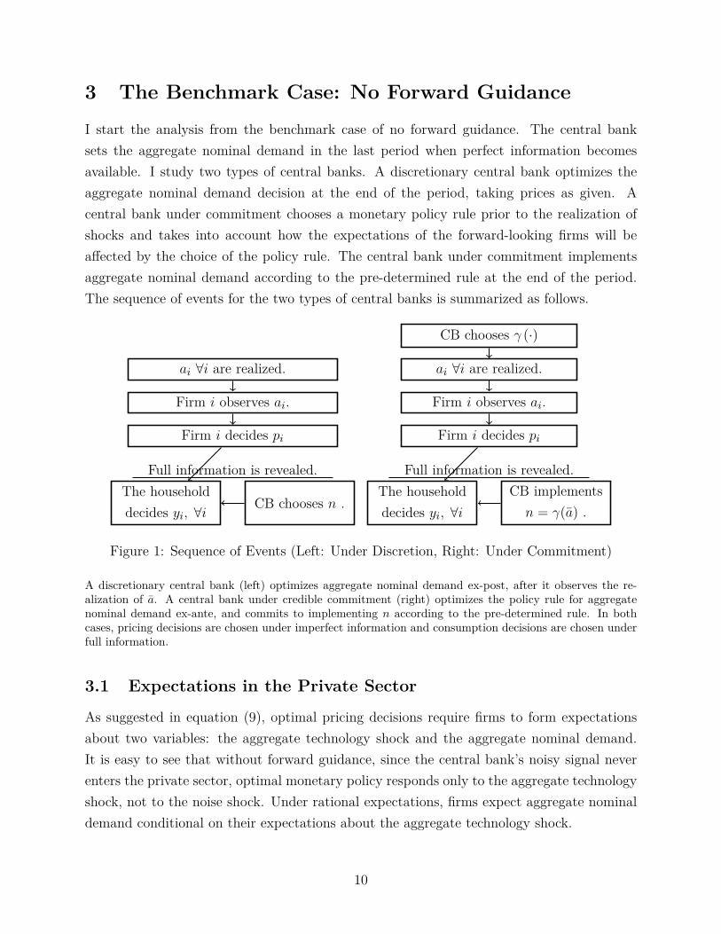
I start the analysis from the benchmark case of no forward guidance. The central banksets the aggregate nominal demand in the last period when perfect information becomesavailable. I study two types of central banks. A discretionary central bank optimizes theaggregate nominal demand decision at the end of the period, taking prices as given. Acentral bank under commitment chooses a monetary policy rule prior to the realization ofshocks and takes into account how the expectations of the forward-looking firms will beaffected by the choice of the policy rule. The central bank under commitment implementsaggregate nominal demand according to the pre-determined rule at the end of the period.The sequence of events for the two types of central banks is summarized as follows.

ai ∀i are realized.

Firm i observes ai.

Firm i decides pi

The householddecides yi, ∀i

CB chooses n .

Full information is revealed.

CB chooses γ (·)


Firm i observes ai.

Firm i decides pi


CB implementsn = γ(a) .


Figure 1: Sequence of Events (Left: Under Discretion, Right: Under Commitment)

A discretionary central bank (left) optimizes aggregate nominal demand ex-post, after it observes the re-alization of a. A central bank under credible commitment (right) optimizes the policy rule for aggregatenominal demand ex-ante, and commits to implementing n according to the pre-determined rule. In bothcases, pricing decisions are chosen under imperfect information and consumption decisions are chosen underfull information.

3.1 Expectations in the Private Sector

As suggested in equation (9), optimal pricing decisions require firms to form expectationsabout two variables: the aggregate technology shock and the aggregate nominal demand.It is easy to see that without forward guidance, since the central bank’s noisy signal neverenters the private sector, optimal monetary policy responds only to the aggregate technologyshock, not to the noise shock. Under rational expectations, firms expect aggregate nominaldemand conditional on their expectations about the aggregate technology shock.

10

Without forward guidance, the information set of each firm consists only of its firm-specific technology, ωi = {ai}. Firms weigh their private signals and their prior beliefs (theex-ante mean of a) to form expectations about the aggregate technology shock. The expectedaggregate technology shock formed by firm i is given by

Eia= κsκs+κa

ai+κa

κs+κaµa = κs

κs+κaai, (11)

where κs = 1/σ2s denotes the precision of private signals, and κa = 1/σ2

a denotes the precisionof the prior.

The optimal price is determined by higher-order beliefs, which are solved by first takingthe average of individual beliefs,

Ea= κsκs+κa

a. (12)

and then taking Ei over this first-order averaged expectation. Iterating this process yieldshigher-order expectations to be:

EiEj a=

(κs

κs+κa

)j+1ai. (13)

For a discretionary central bank, I guess and verify that optimal discretionary policy islinear to the aggregate technology shock.6 For a central bank under commitment, I studythe set of monetary policy rules that respond linearly to the aggregate technology shock.For both types of central banks, the aggregate nominal demand follows,

n= γa. (14)

where γ is optimally chosen in both cases.The expected aggregate nominal demand is thus given by

Ein= γEia= κsκs+κa

γai. (15)6Specifically, I first guess that firms expect aggregate nominal demand to be linear to the aggregate

technology shock, and then solve for the optimal discretionary monetary policy, which turns out to be linearto the aggregate technology shock, consistent with the firms’ expectations.

11

3.2 The Optimal Monetary Policy

The central bank’s ex-ante loss function is the expected weighted sum of the squared outputgap and the squared price level, which is given by

E [L] = E[(y−yeff

)2+ τp2

], (16)

where yeff , the efficient level of output, is defined as the output level when information isperfect (specified in equation (19)).

Before diving into how optimal monetary policy depends on the information frictions inthe private sector, let us first consider the following two extreme cases:

Extreme Case I - Perfect Information about the Aggregate Technology ShockWhen the precision of private signals approaches infinity, the economy approaches the

perfect information case. To find the equilibrium price and output level in this case, substi-tute Eia= a and Ein= n= γa into equation (9), and then apply y = n−p. The equilibriumprice and the output level are shown to be:

p→ αγ−βα

(17)

y→ β

αa (18)

It shows that the real dichotomy holds, meaning that the output level is independentof the effect of monetary policy. Although monetary policy is set after pricing decisionsare made, the effect of monetary policy is completely on the aggregate price level, not theoutput level. This is because firms are forward looking. Under rational expectations andfull information, firms can perfectly forecast the aggregate nominal demand that will be setin the last stage. Therefore, prices fully adjust to the change in aggregate nominal demand,which leaves monetary policy with no effect on real output. If a central bank wants tominimize price deviations, it can achieve full price stabilization by setting n= β

α a.I define the output level in this case under perfect information to be the efficient output

level, which is given byyeff ≡ y→ β

αa (19)

Extreme Case II - No Information on the Aggregate StateConsider the other extreme case in which the precision of private signals is zero. To find

the equilibrium price and output level, substitute Eia= 0 and n= γa into equation (9), and

12

then apply y = n−p. The equilibrium price and the output level are shown to be:

p→−βa, (20)

y→ (γ+β)a. (21)

In this case, firms adjust prices only to their firm-specific technology shocks, not to anyaggregate variables. Since monetary policy is only expected to respond to the aggregatetechnology shock and firms do not update expectations about the aggregate technologyshock, they do not update expectations about the change in monetary policy. Consequently,monetary policy does not have any effect on the price level and all of the effect is on the outputlevel. The real dichotomy breaks down owning to information frictions. If a central bankwants to minimize the output gap, y−yeff , it can achieve complete output-gap stabilizationby setting n= β

α −βa.It is interesting to compare this with Woodford (2001), where firms have perfect infor-

mation on the state of the economy, but they have imperfect information on the exogenouschange in monetary policy. Consequently, changes in monetary policy affect real output. Inmy model, firms have perfect information on the endogenous response function of monetarypolicy, but they have imperfect information on the state of the economy. The gap betweenthe actual and the expected state of the economy makes a fraction of the actual monetarypolicy an unanticipated shock to the private sector.

The Intermediate CaseWe now turn to the intermediate case, in which both the variance of the actual aggregate

technology shock and the variance of the idiosyncratic shock are non-zero and finite. Af-ter an aggregate technology shock, all firms update their expectations about the aggregatetechnology shock using their private signals. Under imperfect information, all firms under-estimate the aggregate technology shock on average. Specifically, the first-order average ofthe expected aggregate technology shock is given by

∫Eia= κs

κs+κaa < a. (22)

Firm expect monetary policy conditional on their expectations about the aggregate tech-nology shock, which makes them also underestimate the actual change in aggregate nominaldemand. Specifically,

∫Ein=

∫ κsκs+κa

γaidi= κsκs+κa

n < n. (23)

On average, a fraction of the change in monetary policy ( κsκs+κan) is anticipated by firms,

13

and its effect is absorbed in pricing decisions. The rest of the change in monetary policyis unanticipated by firms, and this unanticipated fraction of the policy change affects thereal output level. The equilibrium price level and the output level are summarized in thefollowing proposition.

Proposition 1 When 0< σa <∞, 0< σs <∞ and n= γa, the real dichotomy breaks downand monetary policy affects both the price level and the output level. The equilibrium aggre-gate price and the output level are given by:

p= (αγ−β)κs−βκaκa+ακs

a (24)

y = βκs+ (γ+β)κaκa+ακs

a (25)

Proof: See Appendix B.

Corollary 1.1 If the central bank optimizes under discretion, it minimizes the output gap(defined as the difference between the equilibrium output and the efficient output), and it canachieve complete output-gap stabilization by setting7

ndisc =(β

α−β

)a, (26)

in which case the equilibrium price level and the equilibrium output level follow

p=−βa, (27)

y = β

αa= yeff . (28)

Corollary 1.2 If the central bank sets monetary policy to minimize the price level, it canachieve complete price stabilization by setting

np stab(a) = β

α

κa+κsκs

a, (29)

7Since the optimal discretionary monetary policy closes the output gap, I use the phrase “the optimaldiscretionary monetary policy” and “the output-gap stabilization policy” interchangeably in the rest of thepaper.

14

in which case the equilibrium price level and the equilibrium output level follow

p= 0, (30)

y = β(κa+κs)ακs

a. (31)

Comparing (26) and (29), we find that the policy that stabilizes the price level leaves theoutput gap open. In addition, after an a shock, np stab(a) > ndisc(a), ∀κs. It suggests thatif the central bank wants to stabilize the price level, it has to commit to leaving a positiveoutput gap by making monetary policy more accommodative than what it would be underdiscretion. Information frictions result in the conflict between stabilizing the aggregate pricelevel and closing the output gap.

If the central bank optimizes under credible commitment, it considers how its choice ofpolicy rule affects the expectations of the forward-looking firms and thus affects both theprice level and the output level. The central bank under commitment chooses the monetarypolicy rule, n = γ · a to minimize the ex-ante loss of the central bank specified in equation(16). The first-order condition yields that

y−yeff

p=−τ

(∂p

∂γ

)(∂y

∂γ

)−1, (32)

where

∂p

∂γ= ακsκa+ακs

, (33)

∂y

∂γ= κaκa+ακs

. (34)

Solving the value of γ yields the following proposition.

Proposition 2 When 0< σa <∞, 0< σs <∞, the optimal monetary policy rule that min-imizes the ex-ante loss function of the central bank is

γ∗ =(κ2a+ τα2κ2

s

)−1(ταβκs(κs+κa) +

(β

α−β

)κ2a

). (35)

To implement the optimal monetary policy rule, the central bank commits to leaving theoutput gap open. In addition, the optimal policy rule shifts from output-gap stabilization toprice-level stabilization when the precision of private signals increases from zero to infinity.

Proof: γ as specified in equation (35) is a continuous function of κs, and ∂γ∂κs

> 0. In

15

addition, γ(κs = 0) = γy stab and γ(κs =∞) = γp stab. So, as the precision of private infor-mation (κs) increases, monetary policy changes from the output-gap stabilization policy tothe price-level stabilization policy.8 From equation (25), if γ > γy stab, then y > yeff and|p|< |−βa|, meaning that after a positive output gap, the central bank commits to a positiveoutput gap to reduce price deviations from the equilibrium price under discretion.

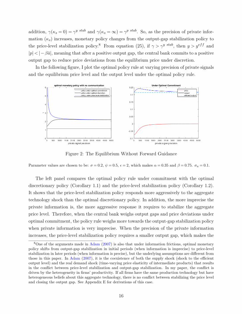
In the following figure, I plot the optimal policy rule at varying precision of private signalsand the equilibrium price level and the output level under the optimal policy rule.

Figure 2: The Equilibrium Without Forward Guidance

Parameter values are chosen to be: σ = 0.2, ψ = 0.5, ε= 2, which makes α= 0.35 and β = 0.75. σa = 0.1.

The left panel compares the optimal policy rule under commitment with the optimaldiscretionary policy (Corollary 1.1) and the price-level stabilization policy (Corollary 1.2).It shows that the price-level stabilization policy responds more aggressively to the aggregatetechnology shock than the optimal discretionary policy. In addition, the more imprecise theprivate information is, the more aggressive response it requires to stabilize the aggregateprice level. Therefore, when the central bank weighs output gaps and price deviations underoptimal commitment, the policy rule weighs more towards the output-gap stabilization policywhen private information is very imprecise. When the precision of the private informationincreases, the price-level stabilization policy requires a smaller output gap, which makes the

8One of the arguments made in Adam (2007) is also that under information frictions, optimal monetarypolicy shifts from output-gap stabilization in initial periods (when information is imprecise) to price-levelstabilization in later periods (when information is precise), but the underlying assumptions are different fromthose in this paper. In Adam (2007), it is the coexistence of both the supply shock (shock to the efficientoutput level) and the real demand shock (time-varying price elasticity of intermediate products) that resultsin the conflict between price-level stabilization and output-gap stabilization. In my paper, the conflict isdriven by the heterogeneity in firms’ productivity. If all firms have the same production technology but haveheterogeneous beliefs about this aggregate technology, there is no conflict between stabilizing the price leveland closing the output gap. See Appendix E for derivations of this case.

16

optimal policy rule shift toward price-level stabilization policy. When the precision of pri-vate information approaches infinity, the real dichotomy holds asymptotically, and the realoutput level is independent of monetary policy. The right panel illustrates the equilibriumprice level and the output gap under the optimal policy rule after a positive aggregate tech-nology shock. As the central bank commits to a more accommodating monetary policy, theequilibrium output is higher than the efficient output and the price deviation is reduced fromthe equilibrium under optimal discretionary policy. As the precision of private informationincreases, the output level approaches the efficient level and the price level approaches zero.

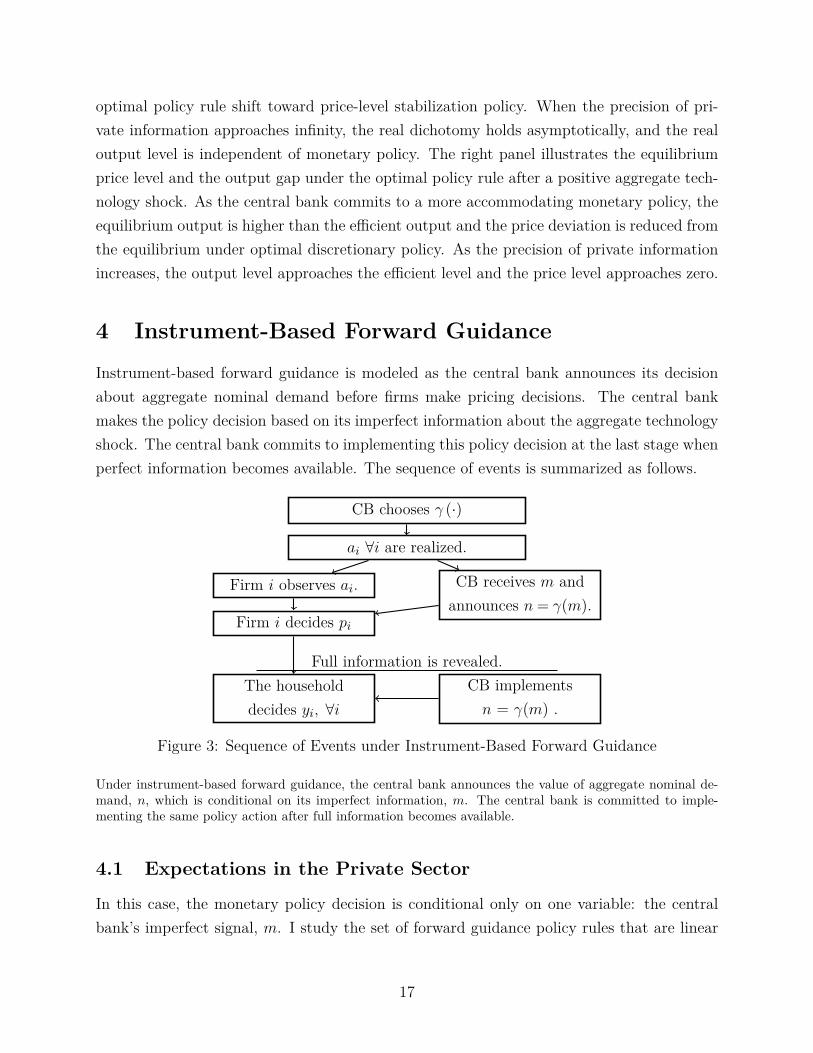
4 Instrument-Based Forward Guidance

Instrument-based forward guidance is modeled as the central bank announces its decisionabout aggregate nominal demand before firms make pricing decisions. The central bankmakes the policy decision based on its imperfect information about the aggregate technologyshock. The central bank commits to implementing this policy decision at the last stage whenperfect information becomes available. The sequence of events is summarized as follows.

CB chooses γ (·)


Firm i observes ai. CB receives m andannounces n = γ(m).

Firm i decides pi


CB implementsn = γ(m) .


Figure 3: Sequence of Events under Instrument-Based Forward Guidance

Under instrument-based forward guidance, the central bank announces the value of aggregate nominal de-mand, n, which is conditional on its imperfect information, m. The central bank is committed to imple-menting the same policy action after full information becomes available.


In this case, the monetary policy decision is conditional only on one variable: the centralbank’s imperfect signal, m. I study the set of forward guidance policy rules that are linear

17

to the central bank’s information, which is given by,

n= γ ·m (36)

Under rational expectations, firms can perfectly infer m when observing n. Upon receiv-ing the public signal provided by the central bank, the information set of individual firmsbecomes ωi = {m, ai}. Firms form conditional expectations on the aggregate technologyshock by weighing the public signal with their private signals,

Eia= κmκm+κs+κa

m+ κsκm+κs+κa

ai. (37)

In the rest of the paper, I denote K ≡ κm +κs +κa. The first-order average expectationacross all firms are: ∫

Eiadi= κmKm+ κs

Ka= κm+κs

Ka+ κm

Kυ (38)

Compared with equation (12), it is easy to see the ex-post trade-off of providing forwardguidance: after a real technology shock, the gap between the averaged expected a and theactual a is reduced by forward guidance. However, the noise shock also drives the expectedtechnology shock away from the actual technology shock.

The higher-order beliefs on a are solved by repeatedly taking the average of expectationsacross i and then applying Ei to the previous average. Specifically, to get the second-orderexpectations from the first order, apply Ei to equation (38) and get:

EiEa= κmKm+ κs

K

(κmKm+ κs

Kai

)=(κmK

+ κsK

κmK

)m+

(κsK

)2ai (39)

Iterate the process to the j-th order, which yields

EiEj−1a=

(κmK

)Σk=jk=1

(κsK

)k−1m+

(κsK

)jai. (40)

When beliefs are taken to higher orders, the weight of the public signal gets amplified.Firms have homogeneous expectations about monetary policy, as they expect the central

bank to implement the same aggregate nominal demand as what is communicated in theforward guidance. Specifically,

Ein= n= γm ∀i (41)

andEiE

j−1n= Ein ∀j (42)

18

4.2 Optimal Monetary Policy

The following proposition describes the equilibrium price and output level under instrument-based forward guidance.

Proposition 3 When instrument-based forward guidance is provided in the form of n= γm,the equilibrium price and output are:9

p=(γ− β

α

ακa+κm+ακsK ′

)a+

(γ− β

α

(1−α)κmK ′

)υ (43)

y = β

α


a+ β

α

(1−α)κmK ′

υ (44)

Proof: The equilibrium aggregate price level is solved by substituting EiEj−1a and

EiEj−1n in equation (9) with equation (40) and in equation (42). The equilibrium output is

solved by taking the difference between the aggregate nominal demand and the equilibriumprice level. See Appendix C for detailed derivations.

Corollary 3.1 Under instrument-based forward guidance, the output level is independent ofthe effect of monetary policy.

As shown in (44) the instrument-based forward guidance affects the real output level onlyby providing an extra source of information, measured by κm. The monetary policy rule, γ,does not affect real output. This is because since the central bank commits to implementingthe monetary policy action provided by the forward guidance, firms have perfect informationon the changes in monetary policy before making pricing decisions. Since prices are perfectlyflexible, prices fully adjust to changes in monetary policy, leaving no effect on the real output.

Corollary 3.2 Under instrument-based forward guidance, the output gap is negative after apositive technology shock and is positive after a positive noise shock.

Since the output level is independent of the effect of monetary policy, there is no trade-offbetween price deviations and output gaps under instrument-based forward guidance. Theoutput level is the result of information frictions. After a positive aggregate technologyshock, firms underestimate the aggregate technology shock, and therefore the output level islower than the efficient level. After a positive noise shock, firms overestimate the aggregatetechnology shock, and therefore the output level is higher than the efficient level.

9In the rest of the paper, I denote K′ = κa+κm+ακs.

19

Under instrument-based forward guidance, the equilibrium in the private sector changesin response to not only the aggregate technology shock but also to the noise in the centralbank’s information. The central bank’s ex-ante loss function becomes

E[L] = E[(y−yeff

)2+ τp2

]≡∫ ∫ [(

y−yeff)2

+ τp2]dadε (45)

where yeff is defined in equation (19). Since the real output level is independent of thechoice of monetary policy, the optimization problem reduces to choosing the policy rule tominimize ex-ante price fluctuations, which is given by

maxn=γmE[p2]. (46)

The first-order condition on γ yields

p(a)p(υ) =−σ

2υ

σ2a. (47)

The following proposition describes the optimal instrument-based forward guidance.

Proposition 4 The optimal instrument-based forward guidance minimizes ex-ante price de-viations by targeting a negative ratio between price deviations due to technology shocks andprice deviations due to noise shocks. The optimal policy rule that achieves this target isn= γ∗m and

γ∗ =(σ2a+σ2

υ

)−1(β

α


σ2a+ β

α

(1−α)κmK ′

σ2ε

). (48)

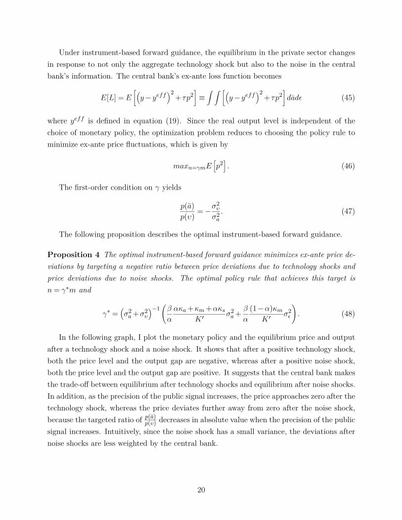
In the following graph, I plot the monetary policy and the equilibrium price and outputafter a technology shock and a noise shock. It shows that after a positive technology shock,both the price level and the output gap are negative, whereas after a positive noise shock,both the price level and the output gap are positive. It suggests that the central bank makesthe trade-off between equilibrium after technology shocks and equilibrium after noise shocks.In addition, as the precision of the public signal increases, the price approaches zero after thetechnology shock, whereas the price deviates further away from zero after the noise shock,because the targeted ratio of p(a)

p(υ) decreases in absolute value when the precision of the publicsignal increases. Intuitively, since the noise shock has a small variance, the deviations afternoise shocks are less weighted by the central bank.

20

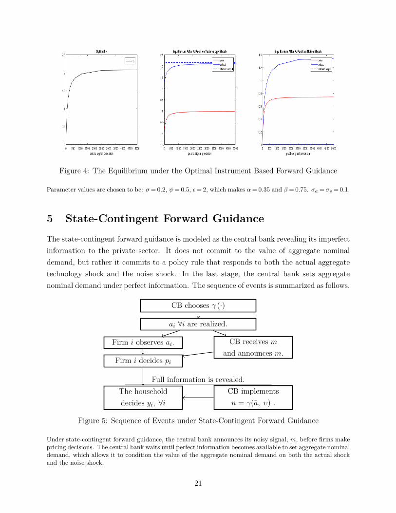
Figure 4: The Equilibrium under the Optimal Instrument Based Forward Guidance

Parameter values are chosen to be: σ= 0.2, ψ= 0.5, ε= 2, which makes α= 0.35 and β = 0.75. σa = σs = 0.1.

5 State-Contingent Forward Guidance

The state-contingent forward guidance is modeled as the central bank revealing its imperfectinformation to the private sector. It does not commit to the value of aggregate nominaldemand, but rather it commits to a policy rule that responds to both the actual aggregatetechnology shock and the noise shock. In the last stage, the central bank sets aggregatenominal demand under perfect information. The sequence of events is summarized as follows.

CB chooses γ (·)


Firm i observes ai. CB receives mand announces m.

Firm i decides pi


CB implementsn = γ(a, υ) .


Figure 5: Sequence of Events under State-Contingent Forward Guidance

Under state-contingent forward guidance, the central bank announces its noisy signal, m, before firms makepricing decisions. The central bank waits until perfect information becomes available to set aggregate nominaldemand, which allows it to condition the value of the aggregate nominal demand on both the actual shockand the noise shock.

21


In this case, the monetary policy decision is conditional on two aggregate variables: theactual aggregate technology shock and the noise shock. I study the set of policy rules thatrespond linearly to the two shocks, which is given by

n= γaa+γυυ. (49)

Note that this function nests the case of instrument-based forward guidance, in whichcase γa = γυ, and nests the case of no forward guidance, in which case γυ = 0.

As long as γa 6= γυ and γυ 6= 0, to form expectations about aggregate nominal demand,firms need to form expectations about both the actual shock and the noise shock as well.

Expectations about the Actual ShockUnder state-contingent forward guidance, the information set of individual firms is the

same as the one under instrument-based forward guidance. Expectations about the aggregatetechnology shock are formed in the same way, which is given by equation (40).

Expectations about the Noise in the Public SignalFirms form expectations about the noise shock by subtracting their expected a from the

the public signal, which is given by

Eiυ = Ei (m− a) =m−Eia. (50)

Substitute Eia in the above equation with equation (37) to get the average expected noiseshock, which is given by:

∫Eiυdi=m− κm+κs

κa+κm+κsa= κa

κa+κm+κsa+ κa+κs

κa+κm+κsυ (51)

It suggests that if the public signal provided by the central bank turns out to be a noise shock,the more precise the public signal is, the less private agents expect it to be a noise shock.Equivalently speaking, a noise shock misleads the private sector to expect an aggregatetechnology shock, and this effect is stronger the more precise the central bank’s informationis.

Expectations about Aggregate Nominal DemandTo form expectations about aggregate nominal demand, apply Ei to equation (49) and

then substitute Eia with equation (40) and Eiυ with equation (51).

Ein=(γa

κmκm+κs+κa

+γυκs+κa

κm+κs+κa

)m+

((γa−γv) κs

κm+κs+κa

)ai (52)

22

In the rest of the paper, I simplify (52) as:

Ein= ρmm+ρaai (53)

where ρm = γa κmκm+κs+κa +γυ κs+κa

κm+κs+κa , and ρa = (γa−γv) κsκm+κs+κa .

To calculate the higher-order beliefs on aggregate nominal demand, start by taking thefirst-order average of expectations, which is given by

En= (ρm+ρa)a+ρmυ. (54)

and then applying Ei to the above equation as:

EiEn= ρmm+ρaEia= ρmm+ρa

(κmKm+ κs

Kai

). (55)

It shows that the weight on the public signal is amplified when beliefs about aggregatenominal demand are taken to the higher order. Continuing this process to get the j− thorder beliefs on the nominal aggregate demand:

EiEjn= ρmm+ρaEiE

j−1a. (56)

5.2 Optimal Monetary Policy

The following proposition describes the equilibrium price and output level under state-contingent forward guidance.

Proposition 5 When state-contingent forward guidance is provided in the form of n= γaa+γvυ, the equilibrium price and the output are:

p= (φm+φa)a+φmυ (57)

y = (γa−φm−φa)a+ (γυ−φm)υ (58)

23

where

φm = ρm+[ρa(1−α)−β 1−α

α

]κm

ακs+κa+κm(59)

φa = [αρa−β] (1−α)κsκm+κa+ακs

+αρa−β (60)

ρm = γaκm

κm+κs+κa+γυ

κs+κaκm+κs+κa

(61)

ρa = (γa−γv) κsκm+κs+κa

(62)

Proof: See Appendix D.Before solving for the optimal monetary policy rule, first consider the case of a dis-

cretionary central bank that has no credible commitment to leaving the output gap openex-post. Specifically, a discretionary central bank is expected to achieve y = yeff after theactual technology shock and y= 0 after the noise shock. The following corollary characterizesthe output gap stabilization policy.

Corollary 5.1 The condition for complete output-gap stabilization after both technologyshocks and noise shocks is

γa−γυ = β

α−β, (63)

which does not yield a unique solution for {γa, γυ}.

Proof: See Appendix C.Since closing the output gap only requires the difference of γa and γυ to be a constant,

discretionary monetary policy has an extra degree of freedom, which allows the centralbank to seek to minimize price deviations while keeping the output gap closed. Define theoptimal discretionary monetary policy to be the one that minimizes ex-ante price deviationswhile keeping the output gap closed after both technology shocks and noise shocks. Theoptimal discretionary policy is solved by backward induction: in the last stage, the centralbank chooses the set of output-gap stabilization policies that close the output gap (defined inCorollary 5.1). In the first stage, the central bank chooses among the output-gap stabilizationpolicies to minimize the ex-ante price fluctuations. The following corollary summarizes theoptimal discretionary policy with state-contingent forward guidance.

Corollary 5.2 With state-contingent forward guidance, the central bank can reduce ex-anteprice fluctuations while keeping the output gap closed ex-post. The optimization problem ofthe optimal discretionary policy under state-contingent forward guidance is given by

maxn=γaa+γυυ−E[p2]

(64)

24

subject to the optimization result in the second stage, which is given by equation (63). p

follows equation (57) with parameters given by equations (59) to (62).

The optimization problem of the optimal discretionary monetary policy with state-contingent forward guidance becomes similar to the optimal policy rule with instrument-based forward guidance in the sense that the central bank minimizes ex-ante price devia-tions. The difference is that while under the optimal instrument-based forward guidance thecentral bank has no control over the output gap ex-post, the optimal discretionary monetarypolicy with state-contingent forward guidance can close the output gap ex-post thanks tothe additional degree of freedom.

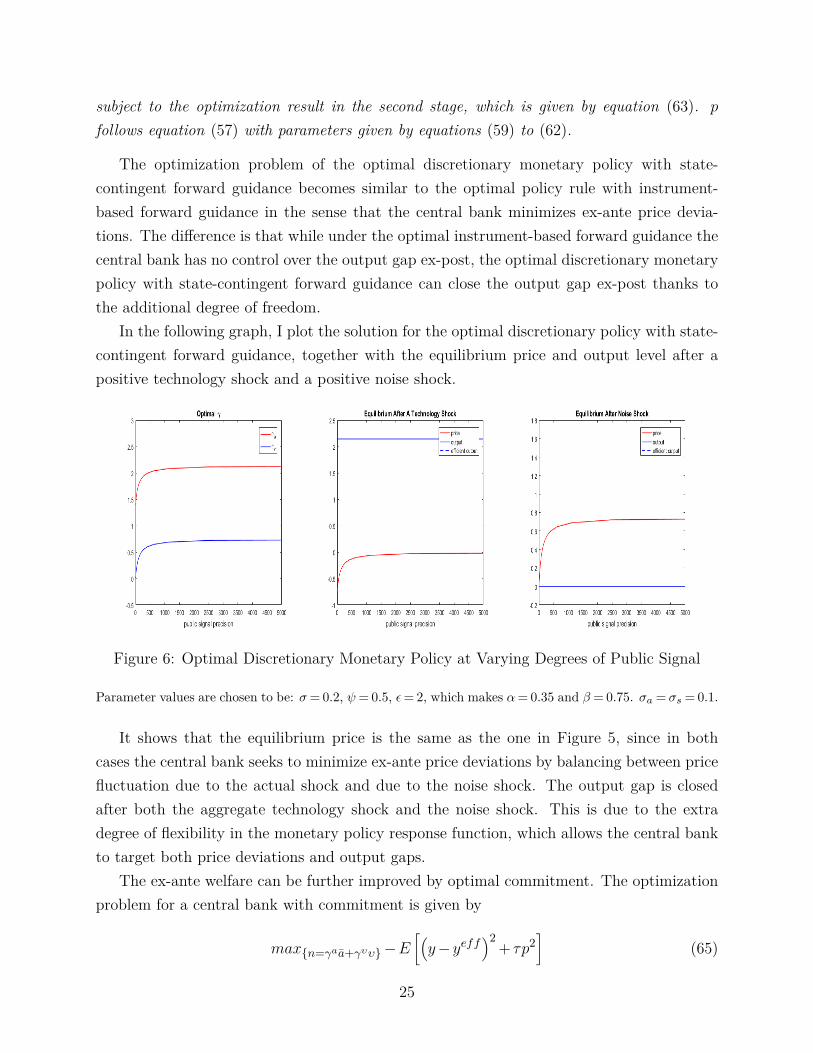
In the following graph, I plot the solution for the optimal discretionary policy with state-contingent forward guidance, together with the equilibrium price and output level after apositive technology shock and a positive noise shock.

Figure 6: Optimal Discretionary Monetary Policy at Varying Degrees of Public Signal


It shows that the equilibrium price is the same as the one in Figure 5, since in bothcases the central bank seeks to minimize ex-ante price deviations by balancing between pricefluctuation due to the actual shock and due to the noise shock. The output gap is closedafter both the aggregate technology shock and the noise shock. This is due to the extradegree of flexibility in the monetary policy response function, which allows the central bankto target both price deviations and output gaps.

The ex-ante welfare can be further improved by optimal commitment. The optimizationproblem for a central bank with commitment is given by

max{n=γaa+γυυ}−E[(y−yeff

)2+ τp2

](65)

25

where p and y evolve according to equations (57) and (58) and parameters are specified inequations (59) to (62).

The first-order conditions are given by[y(a)∂y(a)

∂γa+ τp(a)∂p(a)

∂γa

]σ2a+

[y(υ)∂y(υ)

∂γa+ τp(υ)∂p(υ)

∂γa

]σ2υ = 0 (66)[

y(a)∂y(a)∂γυ

+ τp(a)∂p(a)∂γυ

]σ2a+

[y(υ)∂y(υ)

∂γυ+ τp(υ)∂p(υ)

∂γυ

]σ2υ = 0 (67)

where all derivatives to γ are functions of σa, σs and συ. Details are provided in Appendix D.The following proposition characterizes the optimal policy rule with state-contingent forwardguidance.

Proposition 6 The optimal state-contingent forward guidance minimizes the ex-ante loss bycommitting to a negative ratio between the weighted sum of deviations of the output gap andthe price level after the actual aggregate technology shock and the weighted sum of deviationsafter the noise shock.

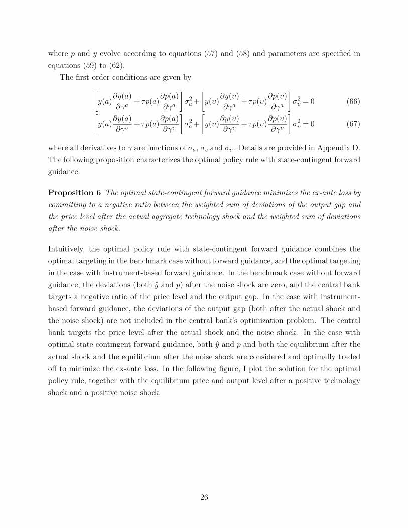
Intuitively, the optimal policy rule with state-contingent forward guidance combines theoptimal targeting in the benchmark case without forward guidance, and the optimal targetingin the case with instrument-based forward guidance. In the benchmark case without forwardguidance, the deviations (both y and p) after the noise shock are zero, and the central banktargets a negative ratio of the price level and the output gap. In the case with instrument-based forward guidance, the deviations of the output gap (both after the actual shock andthe noise shock) are not included in the central bank’s optimization problem. The centralbank targets the price level after the actual shock and the noise shock. In the case withoptimal state-contingent forward guidance, both y and p and both the equilibrium after theactual shock and the equilibrium after the noise shock are considered and optimally tradedoff to minimize the ex-ante loss. In the following figure, I plot the solution for the optimalpolicy rule, together with the equilibrium price and output level after a positive technologyshock and a positive noise shock.

26

Figure 7: The Equilibrium Under the Optimal State-Contingent Forward Guidance


It shows that after a positive aggregate technology shock, the output gap is positivewhile the price level is negative, similar to case without forward guidance, where the optimalpolicy rule targets a negative ratio between the output gap and the price level after theactual technology shock. After a positive noise shock, the price level is positive, similar tothe case with instrument-based forward guidance, where the optimal monetary policy targetsa negative ratio between price deviations after the actual shock and price deviations afterthe noise shock.

6 Ex-ante Welfare Comparison

There should be no surprise that the ex-ante welfare is maximized (equivalently speaking, theex-ante loss is minimized) under the optimal state-contingent forward guidance, since boththe benchmark case without forward guidance and the instrument-based forward guidanceare the results of the same optimization problem but with restrictions on the set of policychoices. (The benchmark case restricts γυ = 0 and the instrument based forward guidancerestricts γa = γυ.)

Whether providing the optimal instrument-based forward guidance improves ex-ante wel-fare from the benchmark case without forward guidance depends on the precision of thecentral bank’s information. In the following figure, I plot the ex-ante loss for the three casesat varying precisions of the central bank’s information. For the optimal instrument-basedforward guidance, the ex-ante loss of losing control over the output level is higher whenthe central bank’s information is less precise, and outweighs the benefits of being able to

27

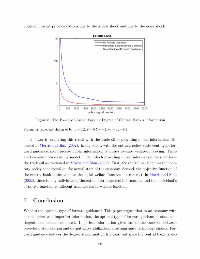
optimally target price deviations due to the actual shock and due to the noise shock.

Figure 8: The Ex-ante Loss at Varying Degree of Central Bank’s Information

Parameter values are chosen to be: σ = 0.2, ψ = 0.5, ε= 2, σa = σs = 0.1

It is worth comparing this result with the trade-off of providing public information dis-cussed in Morris and Shin (2002). In my paper, with the optimal policy state-contingent for-ward guidance, more precise public information is always ex-ante welfare-improving. Thereare two assumptions in my model, under which providing public information does not havethe trade-off as discussed in Morris and Shin (2002). First, the central bank can make mone-tary policy conditional on the actual state of the economy. Second, the objective function ofthe central bank is the same as the social welfare function. In contrast, in Morris and Shin(2002), there is only individual optimization over imperfect information, and the individual’sobjective function is different from the social welfare function.

7 Conclusion

What is the optimal type of forward guidance? This paper argues that in an economy withflexible prices and imperfect information, the optimal type of forward guidance is state con-tingent, not instrument based. Imperfect information gives rise to the trade-off betweenprice-level stabilization and output-gap stabilization after aggregate technology shocks. For-ward guidance reduces the degree of information frictions, but since the central bank is also

28

subject to imperfect information, forward guidance also introduces a noise shock that comesfrom the central bank’s own information.

The key message is that this noise shock gives the monetary policy function an extradegree of freedom. The central bank can reduce ex-ante price deviations by targeting theoptimal trade-off between price deviations after the actual shock and price deviations afterthe noise shock. However, this benefit comes with a cost if forward guidance is instrumentbased. This is because since the central bank announces the value of aggregate nominaldemand before firms set prices, prices will fully adjust to changes in monetary policy, leavingthe output level independent of the effect of monetary policy. This cost is greater ex-antewhen the central bank’s information is less precise.

The optimal state-contingent forward guidance maximizes the ex-ante welfare by com-bining optimal commitment in two ways. First, it targets the optimal trade-off betweenthe price level and the output gap - the same as the optimal policy rule without forwardguidance. Second, it targets the optimal trade-off between deviations after the actual shockand deviations after the noise shock - the same as the optimal instrument-based forwardguidance.

29

References

Acharya, Sushant and Keshav Dogra. 2018. “Understanding HANK: Insights from aPRANK.” FRB of New York Staff Report (835).

Adam, Klaus. 2007. “Optimal Monetary Policy with Imperfect Common Knowledge.” Jour-nal of monetary Economics 54 (2):267–301. URL https://doi.org/10.1016/j.jmoneco.2005.08.020.

Andrade, Philippe, Gaetano Gaballo, Eric Mengus, and Benoit Mojon. 2019. “Forward Guid-ance and Heterogeneous Beliefs.” American Economic Journal: Macroeconomics 11 (3):1–29. URL https://doi.org/10.1257/mac.20180141.

Angeletos, George-Marios and Jennifer La’O. 2010. “Noisy Business Cycles.” NBER Macroe-conomics Annual 24 (1):319–378. URL https://doi.org/10.1086/648301.

———. 2019. “Optimal Monetary Policy with Informational Frictions.” Journal of PoliticalEconomy :704758URL https://doi.org/10.1086/704758.

Angeletos, George-Marios and Chen Lian. 2018. “Forward Guidance without CommonKnowledge.” American Economic Review 108 (9):2477–2512. URL https://doi.org/10.1257/aer.20161996.

Angeletos, George-Marios and Karthik A Sastry. 2018. “Managing Expectations withoutRational Expectations.” Working Paper 25404, National Bureau of Economic Research.URL https://doi.org/10.3386/w25404.

Baeriswyl, Romain and Camille Cornand. 2010. “The Signaling Role of Policy Actions.”Journal of Monetary Economics 57 (6):682–695. URL https://doi.org/10.1016/j.jmoneco.2010.06.001.

Ball, Laurence, N Gregory Mankiw, and Ricardo Reis. 2005. “Monetary Policy for InattentiveEconomies.” Journal of monetary economics 52 (4):703–725. URL https://doi.org/10.1016/j.jmoneco.2005.03.002.

Barro, Robert J and David B Gordon. 1983. “Rules, Discretion and Reputation in a Modelof Monetary Policy.” Journal of monetary economics 12 (1):101–121. URL https://doi.org/10.1016/0304-3932(83)90051-X.

Bassetto, Marco. 2019. “Forward Guidance: Communication, Commitment, or Both?” Jour-nal of Monetary Economics URL https://doi.org/10.1016/j.jmoneco.2019.08.015.

30

https://doi.org/10.1016/j.jmoneco.2005.08.020


https://doi.org/10.1257/mac.20180141

https://doi.org/10.1086/648301

https://doi.org/10.1086/704758

https://doi.org/10.1257/aer.20161996

https://doi.org/10.1257/aer.20161996

https://doi.org/10.3386/w25404





https://doi.org/10.1016/0304-3932(83)90051-X

https://doi.org/10.1016/0304-3932(83)90051-X


Bilbiie, Florin O. 2019. “Optimal Forward Guidance.” American Economic Journal: Macroe-conomics 11 (4):310–45. URL https://doi.org/10.1257/mac.20170335.

Campbell, Jeffrey R, Charles L Evans, Jonas DM Fisher, Alejandro Justiniano, Charles WCalomiris, and Michael Woodford. 2012. “Macroeconomic Effects of Federal Reserve For-ward Guidance [with Comments and Discussion].” Brookings Papers on Economic Activity:1–80URL https://doi.org/10.1353/eca.2012.0004.

Campbell, Jeffrey R, Filippo Ferroni, Jonas DM Fisher, and Leonardo Melosi. 2019.“The Limits of Forward Guidance.” URL https://doi.org/10.1016/j.jmoneco.2019.08.009.

Carlstrom, Charles T, Timothy S Fuerst, and Matthias Paustian. 2015. “Inflation and Outputin New Keynesian Models with a Transient Interest Rate Peg.” Journal of MonetaryEconomics 76:230–243. URL https://doi.org/10.1016/j.jmoneco.2015.09.004.

Del Negro, Marco, Marc P Giannoni, and Christina Patterson. 2012. “The Forward GuidancePuzzle.” FRB of New York Staff Report (574).

Eggertsson, Gauti and Michael Woodford. 2003. “The Zero Bound on Interest Rates andOptimal Monetary Policy.” Brookings Papers on Economic Activity 34 (1):139–235. URLhttps://doi.org/10.1353/eca.2003.0010.

Farhi, Emmanuel and Iván Werning. 2017. “Monetary Policy, Bounded Rationality, andIncomplete Markets.” Working Paper 23281, National Bureau of Economic Research.URL https://doi.org/10.3386/w23281.

Gabaix, Xavier. 2016. “A Behavioral New Keynesian Model.” Working Paper 22954, NationalBureau of Economic Research. URL https://doi.org/10.3386/w22954.

Jia, Chengcheng. 2019. “The Informational Effect of Monetary Policy and the Case forPolicy Commitment.” Federal Reserve Bank of Cleveland, Working Paper 19 (07). URLhttps://doi.org/10.26509/frbc-wp-201907.

Kaplan, Greg, Benjamin Moll, and Giovanni L Violante. 2018. “Monetary Policy Accordingto HANK.” American Economic Review 108 (3):697–743. URL https://doi.org/10.1257/aer.20160042.

Kydland, Finn E. and Edward C. Prescott. 1977. “Rules Rather than Discretion: TheInconsistency of Optimal Plans.” Journal of Political Economy 85 (3):473–491. URLhttps://doi.org/10.1086/260580.

31

https://doi.org/10.1257/mac.20170335

https://doi.org/10.1353/eca.2012.0004




https://doi.org/10.1353/eca.2003.0010



https://doi.org/10.26509/frbc-wp-201907

https://doi.org/10.1257/aer.20160042

https://doi.org/10.1257/aer.20160042

https://doi.org/10.1086/260580

Lorenzoni, Guido. 2010. “Optimal Monetary Policy with Uncertain Fundamentals and Dis-persed Information.” The Review of Economic Studies 77 (1):305–338. URL https://doi.org/10.1111/j.1467-937X.2009.00566.x.

Lucas, Robert E. 1972. “Expectations and the Neutrality of Money.” Journal of economictheory 4 (2):103–124. URL https://doi.org/10.1016/0022-0531(72)90142-1.

McKay, Alisdair, Emi Nakamura, and Jón Steinsson. 2016. “The Power of Forward GuidanceRevisited.” American Economic Review 106 (10):3133–58. URL https://doi.org/10.1257/aer.20150063.

Morris, Stephen and Hyun Song Shin. 2002. “Social Value of Public Informa-tion.” american economic review 92 (5):1521–1534. URL https://doi.org/10.1257/000282802762024610.

Nimark, Kristoffer. 2008. “Dynamic pricing and imperfect common knowledge.” Journal ofmonetary Economics 55 (2):365–382. URL https://doi.org/10.1016/j.jmoneco.2007.12.008.

Paciello, Luigi and Mirko Wiederholt. 2013. “Exogenous Information, Endogenous Informa-tion, and Optimal Monetary Policy.” Review of Economic Studies 81 (1):356–388. URLhttps://doi.org/10.1093/restud/rdt024.

Phelps, Edmund S. 1970. “Microeconomic Foundations of Employment and Inflation The-ory.” .

Tang, Jenny. 2013. “Uncertainty and the Signaling Channel of Monetary Policy.” .

Woodford, Michael. 2001. “Imperfect Common Knowledge and the Effects of MonetaryPolicy.” Working Paper 8673, National Bureau of Economic Research. URL https://doi.org/10.3386/w8673.

32

https://doi.org/10.1111/j.1467-937X.2009.00566.x

https://doi.org/10.1111/j.1467-937X.2009.00566.x

https://doi.org/10.1016/0022-0531(72)90142-1

https://doi.org/10.1257/aer.20150063

https://doi.org/10.1257/aer.20150063

https://doi.org/10.1257/000282802762024610

https://doi.org/10.1257/000282802762024610



https://doi.org/10.1093/restud/rdt024



Appendices

A Equilibrium in the Private Sector

A.1 Household Optimization Problem

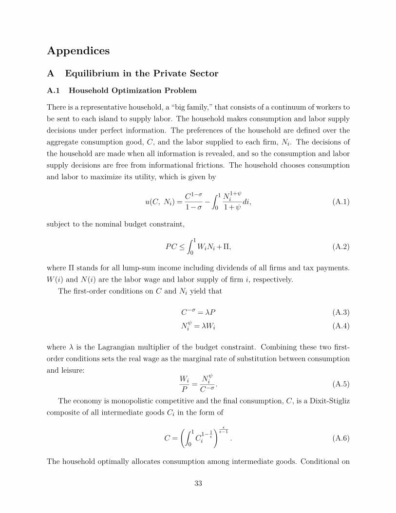
There is a representative household, a “big family,” that consists of a continuum of workers tobe sent to each island to supply labor. The household makes consumption and labor supplydecisions under perfect information. The preferences of the household are defined over theaggregate consumption good, C, and the labor supplied to each firm, Ni. The decisions ofthe household are made when all information is revealed, and so the consumption and laborsupply decisions are free from informational frictions. The household chooses consumptionand labor to maximize its utility, which is given by

u(C, Ni) = C1−σ

1−σ −∫ 1

0

N1+ψi

1 +ψdi, (A.1)

subject to the nominal budget constraint,

PC ≤∫ 1

0WiNi+ Π, (A.2)

where Π stands for all lump-sum income including dividends of all firms and tax payments.W (i) and N(i) are the labor wage and labor supply of firm i, respectively.

The first-order conditions on C and Ni yield that

C−σ = λP (A.3)

Nψi = λWi (A.4)

where λ is the Lagrangian multiplier of the budget constraint. Combining these two first-order conditions sets the real wage as the marginal rate of substitution between consumptionand leisure:

Wi

P= Nψ

i

C−σ. (A.5)

The economy is monopolistic competitive and the final consumption, C, is a Dixit-Stiglizcomposite of all intermediate goods Ci in the form of

C =(∫ 1

0C

1− 1ε

i

) εε−1

. (A.6)

The household optimally allocates consumption among intermediate goods. Conditional on

33

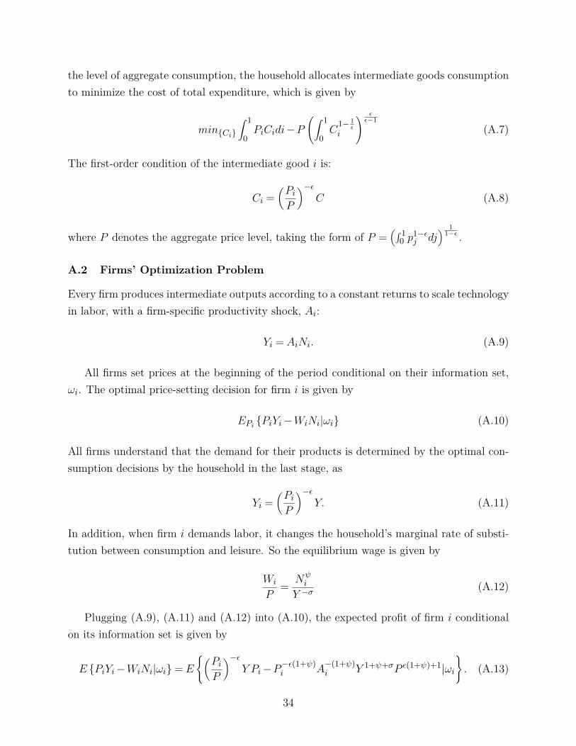
the level of aggregate consumption, the household allocates intermediate goods consumptionto minimize the cost of total expenditure, which is given by

min{Ci}

∫ 1

0PiCidi−P

(∫ 1

0C

1− 1ε

i

) εε−1

(A.7)

The first-order condition of the intermediate good i is:

Ci =(PiP

)−εC (A.8)

where P denotes the aggregate price level, taking the form of P =(∫ 1

0 p1−εj dj

) 11−ε .

A.2 Firms’ Optimization Problem

Every firm produces intermediate outputs according to a constant returns to scale technologyin labor, with a firm-specific productivity shock, Ai:

Yi = AiNi. (A.9)

All firms set prices at the beginning of the period conditional on their information set,ωi. The optimal price-setting decision for firm i is given by

EPi {PiYi−WiNi|ωi} (A.10)

All firms understand that the demand for their products is determined by the optimal con-sumption decisions by the household in the last stage, as

Yi =(PiP

)−εY. (A.11)

In addition, when firm i demands labor, it changes the household’s marginal rate of substi-tution between consumption and leisure. So the equilibrium wage is given by

Wi

P= Nψ

i

Y −σ(A.12)

Plugging (A.9), (A.11) and (A.12) into (A.10), the expected profit of firm i conditionalon its information set is given by

E {PiYi−WiNi|ωi}= E

{(PiP

)−εY Pi−P−ε(1+ψ)

i A−(1+ψ)i Y 1+ψ+σP ε(1+ψ)+1|ωi

}. (A.13)

34

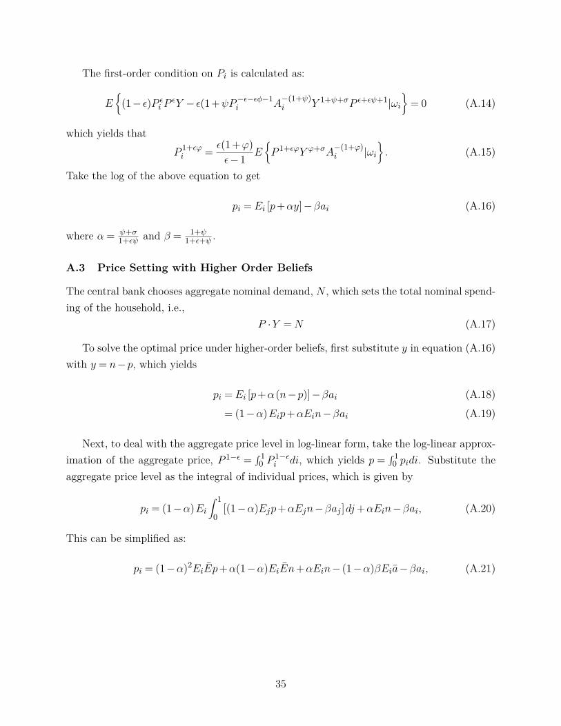
The first-order condition on Pi is calculated as:

E{

(1− ε)P εi P εY − ε(1 +ψP−ε−εφ−1i A

−(1+ψ)i Y 1+ψ+σP ε+εψ+1|ωi

}= 0 (A.14)

which yields thatP 1+εϕi = ε(1 +ϕ)

ε−1 E{P 1+εϕY ϕ+σA

−(1+ϕ)i |ωi

}. (A.15)

Take the log of the above equation to get

pi = Ei [p+αy]−βai (A.16)

where α = ψ+σ1+εψ and β = 1+ψ

1+ε+ψ .

A.3 Price Setting with Higher Order Beliefs

The central bank chooses aggregate nominal demand, N , which sets the total nominal spend-ing of the household, i.e.,

P ·Y =N (A.17)

To solve the optimal price under higher-order beliefs, first substitute y in equation (A.16)with y = n−p, which yields

pi = Ei [p+α (n−p)]−βai (A.18)

= (1−α)Eip+αEin−βai (A.19)

Next, to deal with the aggregate price level in log-linear form, take the log-linear approx-imation of the aggregate price, P 1−ε =

∫ 10 P

1−εi di, which yields p =

∫ 10 pidi. Substitute the

aggregate price level as the integral of individual prices, which is given by

pi = (1−α)Ei∫ 1

0[(1−α)Ejp+αEjn−βaj ]dj+αEin−βai, (A.20)

This can be simplified as:

pi = (1−α)2EiEp+α(1−α)EiEn+αEin− (1−α)βEia−βai, (A.21)

35

where E [·] denotes the average expectation operator in the form of

∫ 1

0Ej (·)dj = E (·) , (A.22)

Ej [·] =∫EiE

j−1 [·]di= EEj−1. (A.23)

Iterating this substitution process leads to the optimal individual price with higher-orderbeliefs:

pi = (1−α)∞EiE∞p+αΣ∞j=0(1−α)jEiEjn−βΣ∞j=0(1−α)j+1EiEj a−βai (A.24)

B The Case Without Forward Guidance

This section derives the aggregate price and output level when the central bank does notprovide forward guidance of any sort, i.e., the central bank does not reveal its imperfectinformation on the aggregate technology shock, nor does it provide its best estimate ofmonetary policy decisions.

B.1 Expectations in the Private Sector

In this case, firms use their private information on the aggregate technology shock to formexpectations about the aggregate technology shock and about the response of monetarypolicy.

Firm i sees only its own technology ai and uses it as the private signal. The conditionalexpectation of the aggregate technology shock becomes

Eia= κsκs+κa

ai+κa

κs+κaµa = κs

κs+κaai (B.1)

To solve for the higher-order beliefs, first take the average over i and get

Ea= κsκs+κa

a. (B.2)

Then apply Ei to this first-order averaged expectation and get

EiEa= κsκs+κa

Eia=(

κsκs+κa

)2ai. (B.3)

36

Continuous iteration of this substitution process finally results in

EiEj a=

(κs

κs+κa

)j+1ai (B.4)

I consider the class of policy rule that is linear to the aggregate technology shock, n= γα,which makes Ein a linear function of Eia, given by Ein= γEia.

Apply (B.4) into (A.24) and get

pi = (1−α)∞EiE∞p+αγΣ∞j=0(1−α)j(

κsκs+κa

)j+1ai−βΣ∞j=0(1−α)j+1

(κs

κs+κa

)j+1ai−βai(B.5)

I guess and verify that the higher-order expectations on p are less than 11−α , which makes

(1−α)∞EiE∞p→ 0. This leads to

pi = (αγ−β)κs−βκaκa+ακs

ai (B.6)

Integration over i results in the equilibrium aggregate price level and output, which aregiven by

p= (αγ−β)κs−βκaκa+ακs

a (B.7)

y = βκs+ (γ+β)κaκa+ακs

a (B.8)

B.2 Optimal Monetary Policy Without Forward Guidance

The central bank chooses the optimal linear policy rule prior to the realization of shocks, tominimize the weighted sum of variances of the price level and the output gap. The objectivefunction of the central bank’s optimization problem is:

minγE[(y−yeff

)2+ τp2

](B.9)

where p and y follow (B.7) and (B.8).The first-order condition on γ is

y−yeff

p=−τ

(∂p

∂γ

)(∂y

∂γ

)−1, (B.10)

which suggests that the optimal policy rule targets a negative ratio between the output gapand the price level.

37

In (B.10), the derivatives of p and y with respect to γ are given by

∂p

∂γ= ακsκa+ακs

, (B.11)

∂y

∂γ= κaκa+ακs

. (B.12)

Substitute these derivatives into equation (B.10) and re-arrange the equation to get

βκs+ (γ+β)κaκa+ακs

= β

α(B.13)

which yields

γ∗ =(κ2a+ τα2κ2

s

)−1(ταβκs(κs+κa) +

(β

α−β

)κ2a

)(B.14)

C Instrument-Based Forward Guidance

C.1 Expectations in the Private Sector

Firms form expectations about the aggregate technology shock by combining the publicsignal from the forward guidance and their private signals. Eia is given by

Eia= κmκm+κs+κξ

m+ κsκm+κs+κξ

ai+κξ

κs+κξµa (C.1)

= κmκm+κs+κξ

m+ κsκm+κs+κξ

ai (C.2)

To get the higher-order beliefs, first integrate over i and get

Ea= κmKm+ κs

Ka (C.3)

where I denote K = κm+κs+κξ. Then apply Ei to the first-order averaged expectations toget:

EiEa= κmKm+ κs

KEia= κm

Km+ κs

K

[κmKm+ κs

Kai

]=[κmK

+ κsK

κmK

]m+

(κsK

)2ai (C.4)

Successive iteration of this process leads to the higher-order beliefs on the aggregate tech-nology:

EiEj−1a=

(κmK

)Σk=jk=1

(κsK

)k−1m+

(κsK

)jai (C.5)

38

Substitute Ein by n and Eia by equation (C.2) into pi, which yields

pi =(γa−β 1−α

α

κmK ′

)m−β K

K ′ai (C.6)

Integrating over i results in the aggregate price level. The real output level is the differencebetween n and p. i.e.,

p=(γ− β

α


)a+

(γ− β

α

(1−α)κmK ′

)υ (C.7)

y = β

α


a+ +β

α

(1−α)κmK ′

υ (C.8)

C.2 Optimal Monetary Policy

The optimal monetary policy then reduces to choose γ to minimize the ex-ante variance ofthe price level, given by

Ep2 =(γa− β

α


)σ2a+

(γa− β

α

(1−α)κmK ′

)συ. (C.9)

The first-order condition yields that

γ− βαακa+κm+ακs

K′

γ− βα

(1−α)κmK′

=−σ2υ

σ2a. (C.10)

Rearrange to get the solution for γ:

γ =(σ2a+σ2

υ

)−1(β

α


σ2a+ β

α

(1−α)κmK ′

σ2ε

)(C.11)

D State-Contingent Forward Guidance

D.1 Expectations in the Private Sector

Firms form expectations about the aggregate technology shock by combining the publicsignal from the forward guidance and their private signals. Eia is given by

Eia= κmκm+κs+κξ

m+ κsκm+κs+κξ

ai+κξ

κs+κξµa (D.1)

= κmκm+κs+κξ

m+ κsκm+κs+κξ

ai (D.2)

39

To get the higher-order beliefs, first integrate over i and get

Ea= κmKm+ κs

Ka (D.3)

where I denote K = κm+κs+κξ. Then apply Ei to the first-order averaged expectations toget:

EiEa= κmKm+ κs

KEia= κm

Km+ κs

K

[κmKm+ κs

Kai

]=[κmK

+ κsK

κmK

]m+

(κsK

)2ai (D.4)

Successive iteration of this process leads to the higher-order beliefs on the aggregate tech-nology:

EiEj−1a=

(κmK

)Σk=jk=1

(κsK

)k−1m+

(κsK

)jai (D.5)

In addition to forming expectations about the aggregate technology shock, firms alsoneed to form expectations about the change in monetary policy. To do so, they also need toform expectations about the noise component in the central bank’s information. Firms formexpectations about the noise shock as the difference between the public signal provided bythe central bank and their own expected a. The expected noise shock is

Eiυ = Ei (m− a) =m−Eia. (D.6)

Substitute Eia by (D.2) and take the average over i:∫Eiυdi=m− κm+κs

κa+κm+κsa= κa

κa+κm+κsa+ κa+κs

κa+κm+κsυ (D.7)

The expected monetary policy is given by

Ein= γaEia+γυEiυ (D.8)

Substitute Eia and Eiυ and get

Ein=(γa

κmκm+κs+κa

+γυκs+κa

κm+κs+κa

)m+

((γa−γv) κs

κm+κs+κa

)ai (D.9)

In the rest of the paper, I simplify (D.9) as:

Ein= ρmm+ρaai (D.10)

where ρm = γa κmκm+κs+κa +γυ κs+κa

κm+κs+κa , and ρa = (γa−γv) κsκm+κs+κa .

40

To solve for the higher-order beliefs, first integrate individual expectations over i, whichyields that ∫ i

0Ein= En= ρmm+ρaa, (D.11)

and then apply Ei to En. Successive iteration results in

EiEjn= ρmm+ρaEiE

j−1a. (D.12)

Having calculated the higher-order beliefs on a and n, we are ready to calculate theequilibrium price. Re-write equation A.24 as:

pi = α[Σ∞j=1(1−α)jEiEjn+Ein

]−βΣ∞j=1(1−α)jEiEj−1a−βai (D.13)

First, substitute EiEjn in the first term by (D.12). The first term becomes

α[Σ∞j=1(1−α)jEiEjn+Ein

]= α

{Σ∞j=1(1−α)j

[ρmm+ρaEiE

j−1a]+ρmm+ρaai

}(D.14)

= α{

Σ∞j=0(1−α)jρmm+ρaΣ∞j=1(1−α)jEiEj−1a+ρaai}

Now, pi is written in terms of public and private signals, which is given by

pi = α

{ρmm

1α

+ρaΣ∞j=1(1−α)j[(κmK

)Σk=jk=1

(κsK

)k−1m+

(κsK

)jai

]+ρaai

}(D.15)

−βΣ∞j=1(1−α)j{(

κmK

)Σk=jk=1

(κsK

)k−1m+

(κsK

)jai

}−βai

To deal with Σ∞j=1(1−α)j{(

κmK

)Σk=jk=1

(κsK

)j−1}, first write out the infinite summation

as

Σ∞j=1(1−α)j{(

κmK

)Σk=jk=1

(κsK

)j−1}= (D.16)

(1−α)κmK

+ (1−α)2κmK

+ (1−α)2κmK

κsK

+ (1−α)3κmK

+ (1−α)3κmK

(κsK

)2+ · · ·

and then collect common terms, which yields that

(1−α)κmK

{Λ1 ·1 +Λ2 ·

κsK

+Λ3 ·(κsK

)2+ · · ·

}(D.17)

41

where Λ1 = 1α , Λ2 = 1−α

α , Λ3 = (1−α)2

α . This leads to

Σ∞j=1(1−α)j{(

κmK

)Σk=jk=1

(κsK

)j−1}= 1−α

α

κmακs+κξ +κm

(D.18)

Substituting this into (D.15) results in

pi =m{ρm+

[ρa(1−α)−β 1−α

α

]κm

ακs+κa+κm

}+ai

{[αρa−β] (1−α)κs

κm+κa+ακs +ρaai−β}(D.19)

Aggregate over i to get the aggregate price level. The aggregate real output is then calculatedas the difference between aggregate nominal demand and the aggregate price level. Theequilibrium p and y are thus given by

p= φmm+φaa= (φm+φa) a+φmυ (D.20)

y = n−p= (γcca −φm−φa) a+ (γccυ −φm)υ (D.21)

where10

φm = ρm+[ρa(1−α)−β 1−α

α

]κmK ′

(D.22)

φa = (αρa−β) KK ′

(D.23)

ρm = γaκmK

+γυκs+κaK

(D.24)

ρa = (γa−γv) κsK

(D.25)

D.2 Output-Gap Stabilization Policy

Proof of Corollary 5.1To close the output gap in the last stage, the central bank chooses {γa, γυ} such that

y = β

αa+ 0 ·υ (D.26)

Comparing coefficients with equation (D.21), we have

γa−φm−φa = β

α(D.27)

γυ−φm = 0 (D.28)10In the rest of the paper, I denote K = κa+κm+κs and K′ = κa+κm+ακs

42

Rearranging terms yields the expressions for {φa, φm}:

φa = γa−γυ− βα

(D.29)

φm = γυ (D.30)

From equation (D.29), substitute φa by equation (D.23):

γa−γυ− βα

= [αρa−β] (1−α)κsκm+κa+ακs

+αρa−β (D.31)

which results in:

ρa =

(γa−γυ− β

α

)K′

K +β

α. (D.32)

Substituting this result into (D.30) results in the expression for ρm given by

ρm = γυ− 1−αα

(γa−γυ− β

α

)κmK

(D.33)

The solutions for (γa, γυ) can be solved by equating the expressions of {ρa, ρm} inequations (D.32) and (D.33) with their expressions in equations (D.24) and (D.25), which isgiven by

(γa−γυ− β

α

)K′

K +β

α= (γa−γυ) κs

K(D.34)

γυ− 1−αα

(γa−γυ− β

α

)κmK

= γaκmK

+γυκa+κaK

(D.35)

By rearranging the two equations we find that the two equations are co-linear in (γa−γυ).So the above two equations only yield the difference between γa and γυ, which is given by

γa−γυ = β

α(1−α) (D.36)

This defines the set of monetary policy that close the output gap in the last stage.

D.3 The Optimal Discretionary Monetary Policy

The optimal discretionary monetary policy is solved by backward induction. The result ofoptimization in the last stage is presented in Corollary 5.1. We now work on the first stage.First, substitute the solution in the last stage, γa−γυ = β

α (1−α) into equations ((D.22) -

43

(D.25)), which results in:

φm = γυ (D.37)

φa =−β (D.38)

ρm = γa−γdκs+κaK

(D.39)

ρa = γdκsK

(D.40)

The equilibrium price and output level under discretionary monetary policy thus become:

p= (γυ−β) a−γυυ (D.41)

y = β

αa+ 0 ·υ (D.42)

The extra degree of flexibility in the policy response function allows the central bank tominimize ex-ante price deviations while keeping the output gap closed ex-post. In this case,the central bank’s objective function reduces to minimizing the ex-ante variance of the pricelevel. The central bank’s objective function then reduces to:

minγυE[p2] =minγv{

(γυ−β)2σ2a+ (γυ)2σ2

v

}(D.43)

The first-order condition on γυ results in

γυ−βγυ

=−σ2v

σ2a

(D.44)

which suggests that the central bank targets a negative ratio between the equilibrium priceafter a shock and the equilibrium price after a noise shock. The absolute value of the ratiois the relative precision of the public signal and the prior of the technology shock.

Solving γυ from the first-order condition results in:

γυ = βσ2a

σ2a+σ2

v(D.45)

D.4 Optimal Policy Rule

The optimal policy rule minimizes the ex-ante loss of the central bank, given by

E[W ] = (γa−φm−φa)2σ2a+ (γυ−φm)2σ2

υ + τ[(φm+φa)2σ2

a+φ2mσ

2υ

](D.46)

The first-order condition on γa results in:

44

σ2a

(γa−φm−φa)d(γa−φm−φa)

dγa+ τ (φm+φa)

d(φm+φa)dγafnc

(D.47)

+σ2υ

(γυ−φm) d(γυ−φm)dγa

+ τφmdφmdγafnc

= 0

Re-arrange the above equation to get:

σ2a

{(γa−φm−φa) + (−γa+ (1 + τ)(φm+φa))

d(φm+φa)dγa

}(D.48)

+σ2υ

(γυ−φm) + (−γυ + (1 + τ)φm) dφmdγafnc

= 0 (D.49)

where

d(φm+φa)dγafnc

= ∂φm∂ρm

∂ρm∂γafnc

+ ∂φm∂ρa

∂ρa∂γafnc

+ ∂φa∂ρm

∂ρm∂γafnc

+ ∂φa∂ρa

∂ρa∂γafnc

(D.50)

dφmdγafnc

= ∂φm∂ρm

∂ρm∂γafnc

+ ∂φm∂ρa

∂ρa∂γafnc

(D.51)

and

∂φm∂ρm

= 1 (D.52)

∂φa∂ρm

= 0 (D.53)

∂φm∂ρa

= (1−α) κmακs+κa+κm

(D.54)

∂φa∂ρa

= αK

K ′(D.55)

∂ρm∂γa

= κmK

(D.56)

∂ρa∂γa

= κsK

(D.57)

∂ρa∂γυ

= κs+κaK

(D.58)

∂ρa∂γυ

=−κsK

(D.59)

The first-order condition on γυ is calculated similarly.

45

E Alternative Assumption: Firms Have Common Technology Shocks

When firms have homogeneous technology but have imperfect information on this commonshock, equation (8) becomes

pi = Ei [p+αy−βa] , (E.1)

as firms also need to guess their own cost of production.Following the same procedure as described in Appendix A, substitute y = n− p into pi

and getpi = (1−α)Eip+αEin−βEia (E.2)

The higher-order beliefs are again solved by first taking the integral of pi to get the aggregateprice level,

p= (1−α)Ep+αEn−βEa (E.3)

and then substituting this expression for p into pi. Iterating this process yields that

pi = (1−α)Ei[(1−α)Ep+αEn−βEa

]+αEin−βEia (E.4)

= (1−α)2EiEp+α(1−α)EiEn+αEin− (1−α)βEiEa+βEia

(E.5)

Taking the expectation about the aggregate technology shock to the infinite order, pibecomes

pi = (1−α)∞EiE∞p+αΣ∞j=0(1−α)jEiEjn−βΣ∞j=0(1−α)jEiEj a (E.6)

whereEiE

j a=(

κsκs+κa

)j+1ai (E.7)

Substituting n= γa and EiEj a into pi yields that

pi = (αγ−β)κsκa+ακs

ai. (E.8)

Take the average of pi and apply y = n−p, which yields the equilibrium price level andthe output level to be

p= (αγ−β)κsκa+ακs

a,

y = γκa+βκsκa+ακs

a.

46

By choosing γ = βα , the central bank closes the output gap and stabilizes the price level

at the same time, meaning that the price stabilization policy is time consistent, and imple-menting the optimal monetary policy does not require credible commitment.

47

Forward Guidance under Imperfect Information: Instrument ...

Documents

Transcript of Forward Guidance under Imperfect Information: Instrument ...