Forward Guidance, Monetary Policy Uncertainty, and …...Forward Guidance, Monetary Policy...

Forward Guidance, Monetary Policy Uncertainty,

and the Term Premium∗

Brent Bundick† Trenton Herriford‡ A. Lee Smith§

July 2017

Abstract

We examine the macroeconomic and term-premia implications of monetary policy

uncertainty shocks. Using Eurodollar options, we employ the VIX methodology to

measure implied volatility about future short-term interest rates at various horizons.

We identify monetary policy uncertainty shocks using the unexpected changes in this

term structure of implied volatility around monetary policy announcements. Two prin-

cipal components succinctly characterize these changes around policy announcements,

which have the interpretation as shocks to the level and slope of the term structure

of implied interest rate volatility. We find that an unexpected decline in the slope of

implied volatility lowers term premia in longer-term bond yields and leads to higher

economic activity and inflation. Our results suggest that forward guidance about future

monetary policy can materially affect bond market term premia, even without large-

scale asset purchases.

JEL Classification: E32, E52

Keywords: Forward Guidance, Policy Uncertainty, Term Premium

∗We thank Courtney Butler and Brett Currier for help in obtaining the Eurodollar options data. The

views expressed herein are solely those of the authors and do not necessarily reflect the views of the Federal

Reserve Bank of Kansas City or the Federal Reserve System.

†Federal Reserve Bank of Kansas City. Email: [email protected]

‡Federal Reserve Bank of Kansas City. Email: [email protected]

§Federal Reserve Bank of Kansas City. Email: [email protected]

1

https://www.kansascityfed.org/people/brentbundick

https://www.kansascityfed.org

https://www.kansascityfed.org/people/andrewleesmith

1 Introduction

With the federal funds rate near zero, the Federal Open Market Committee (FOMC) turned

to forward guidance and large-scale asset purchases (LSAPs) to help stabilize the economy

during and after the Great Recession. In explaining these policies, then Chair Bernanke

stated:

Both LSAPs and forward guidance for the federal funds rate support the econ-

omy by putting downward pressure on longer-term interest rates, but they affect

longer-term rates through somewhat different channels. To understand the dif-

ference, it is useful to decompose longer-term interest rates into two components:

One reflects the expected path of short-term interest rates, and the other is called

a term premium. The term premium is the extra return that investors require to

hold a longer-term security to maturity compared with the expected yield from

rolling over short-term securities for the same period. . .

Forward rate guidance affects longer-term interest rates primarily by influencing

investors’ expectations of future short-term interest rates. LSAPs, in contrast,

most directly affect term premiums. – Bernanke (2013)

However, Michael Woodford uses the following simple example to illustrate why this rigid

dichotomy between these two policy tools and their effects may not be correct in general:

Suppose that FOMC forward guidance were to convince market participants that

there was no possibility of a funds rate above zero for the next ten years . . . An

absence of arbitrage opportunities would require the ten-year zero-coupon yield

to fall to zero – meaning that both the expectations component and the term

premium would be reduced to zero by such a change in expectations about the

short-rate process . . .

Term premia are affected by expectations about the short-rate process (in

particular, the degree of uncertainty about future short rates). – Woodford (2012)

In this paper, we empirically test Woodford’s claim: Do changes in forward guidance alone

significantly affect term premia in bond markets? Specifically, if a forward guidance an-

nouncement causes a decline in uncertainty about future short-term interest rates, does it

also reduce term premia on longer-term bonds?

To answer these questions, we undertake three steps. First, we measure uncertainty

about future short-term interest rates. Second, we isolate exogenous shifts in this measure

2

of uncertainty due to unexpected changes in monetary policy. Finally, we examine the effects

of changes in monetary policy uncertainty on term premia in bond markets. For the first

task of measurement, we develop new, daily frequency measures of uncertainty about future

short-term interest rates over multiple horizons. Specifically, we apply the CBOE Volatility

Index (VIX) methodology to Eurodollar options with various expiration dates. Then, fol-

lowing the recent literature on identifying first-moment monetary policy shocks, we use the

daily changes in our measures around regularly-scheduled FOMC meetings to isolate changes

in interest rate uncertainty attributable to monetary policy. Finally, we use standard event-

study regressions to determine the effects of changes in monetary policy uncertainty on two

different measures of bond market term premia.

We focus our analysis on the 1994–2008 sample period, which avoids the task of disen-

tangling the effects of forward guidance from large-scale asset purchases. While the quotes

of Bernanke and Woodford reference the FOMC’s most recent experience with forward rate

guidance at the zero lower bound, the FOMC previously used its policy statements to in-

fluence expectations about future policy rates. Many times, post-meeting communication

explicitly referenced future policy rates. In other instances, the Committee’s description of

risks surrounding the outlook for growth and inflation implicitly shaped expectations about

future policy rates rate expectations. For the purposes of this paper, we define all such forms

of post-meeting communication as forward guidance since they all could affect the amount

of uncertainty surrounding future policy rates.

We find forward guidance announcements that lower uncertainty about future short rates

lead to statistically significant declines in term premia. Building on the work of Gurkaynak,

Sack and Swanson (2005), we find that two principal components can succinctly capture

changes in the term structure of short-rate volatility around FOMC announcements. These

two components can be interpreted as shocks to the level and slope of the term structure

of implied short-rate volatility. Using an event-study approach around FOMC meetings, we

find an unexpected decline in the slope of implied volatility leads to a significant decline in

bond market term premia of all horizons. Quantitatively, a 5 basis point decline in our slope

factor leads to about a 3 basis point reduction in the ten-year term premium.

Using these estimates from the pre-zero lower bound period, we provide additional evi-

dence that the Committee’s recent date-based guidance was especially effective at shaping

longer-term yields by reducing interest rate uncertainty. At the August 2011 FOMC meet-

ing, the Committee gave very explicit guidance that interest rates were likely to remain

3

near zero “at least through mid-2013.” While the Committee made no changes to the size

or composition of its balance sheet at that meeting, term premia on Treasury securities

declined meaningfully after that announcement. Using our regression model from the 1994–

2008 sample, we show that the observed reduction in uncertainty surrounding future policy

rates alone explains much of this decline in term premia. Thus, we believe our findings based

on the 1994–2008 period remain informative about the effects of the FOMC’s use of forward

guidance after 2008.

Finally, we show that changes in uncertainty surrounding the future path of policy rates

affects both financial markets and the broader macroeconomy. Using a vector autoregression,

we show that declines in future short-rate volatility lead to persistent increases in economic

activity and prices. Following a one standard deviation reduction in the slope of implied

interest rate volatility, industrial production and prices both increase by about 0.30 percent

and the unemployment rate declines by about 5 basis points after about one year. Even after

controlling for surprises in the level of current and future expected interest rates, we find

that changes in uncertainty around the future rate path can significantly impact economic

activity.

2 Simple Theoretical Model

We now describe a simple model which helps guide our intuition and motivates our empirical

specifications. While the model is quite stylized, it delivers two key analytical predictions.

First, consistent with Bernanke’s motivation for the use of unconventional monetary policy

tools, the model predicts that lowering longer-term interest rates leads to higher household

consumption. Second, the model highlights Woodford’s conjecture that uncertainty about

the future short-term interest rates is a key determinant of the term premium.

Our simple model features a representative household which maximizes lifetime expected

utility over consumption Ct. The household receives endowment income et and can purchase

nominal bonds with maturities of 1 to N periods. pnt denotes the price of an n-period bond,

which pays one nominal dollar at maturity (p0t = 1). We denote the aggregate price level

using Pt. The household divides its income between consumption Ct and the amount of the

bonds bnt+1 for n = 1, . . . , N to carry into next period.

Formally, the representative household chooses Ct+s, and bnt+s+1 for all bond maturities

4

n = 1, . . . , N and all future periods s = 0, 1, 2, . . . by solving the following problem:

max Et

∞∑s=0

βs log (Ct+s)

subject to the intertemporal household budget constraint each period,

Ct +N∑

n=1

pntbnt+1

Pt

+ ≤ et +N∑

n=1

pn−1t

bntPt

.

Using a Lagrangian approach, we can derive the following two optimality conditions for the

1- and n-period bonds.

p1t = Et

{βCt

Ct+1

Pt

Pt+1

}(1)

pnt = Et

{βCt

Ct+1

Pt

Pt+1

pn−1t+1

}(2)

We assume that the central bank sets the one-period gross nominal interest rate Rt, which

is equal to the inverse of the one-period bond price p1t . For analytical tractability, we also

make two additional assumptions. First, we assume that all nominal bonds are in zero net

supply. Second, we assume that prices are fixed Pt = P for all t. This second assumption

is not crucial for our main intuition, however, it allows us to derive clear expressions for

longer-term bond yields and the term premium.

Consistent with Bernanke’s intuition, our simple model implies that lowering longer-term

bond yields boost household consumption. After some algebraic manipulation, we can use a

second-order approximation of Equation (2) to derive the following expression:

ct = Et

{ct+n

}− 1

2VARt

{ct+n

}− n

(ynt + log

(β)). (3)

In this equation, ct = log (Ct), VARt denotes the conditional variance, and ynt is the yield to

maturity on an n-period bond.1 Consumption today depends on the expectation and uncer-

tainty about consumption in period t+ n and on the longer-term yield bond. All else equal,

Equation (3) shows that lower long-term bond yields induce higher household consumption.

1A Technical Appendix, available on the Federal Reserve Bank of Kansas City’s webpage, contains a

detailed derivation of all of the equations in Section 2.

5

Moreover, we can decompose the yield to maturity on the n-period bond into two com-

ponents:

ynt ≈1

n

[n−1∑i=0

Et

{rt+i

}+

1

2VARt

{n−1∑i=0

rt+i

}], (4)

where rt = log (Rt) is the net nominal interest rate controlled by the central bank. The first

component depends on both the expected path of short-term nominal interest rates. The

second term reflects the additional compensation the household requires to hold a longer-

term security in the face of an uncertainty about future short-term interest rates.

Following Rudebusch and Swanson (2012), we can derive an expression for the term

premium as the difference between the yield to maturity on the n-period bond and the yield

on a risk-neutral n-period bond, denoted ynt :

TP nt , ynt − ynt ≈

1

nVARt

{n−1∑i=0

rt+i

}. (5)

Equation (5) rigorously formulates Woodford’s simple example: Term premia in our simple

model depend on the uncertainty about the future path of interest rates. Households will

require higher compensation to hold a longer-term bond when they face higher uncertainty

about future short-term interest rates. From a policy perspective, our simple model suggests

that forward guidance announcements that change the uncertainty about future short-term

interest rates should also affect term premia in longer-term nominal bonds.

Our simple model provides two key testable predictions. Motivated by Equation (5),

monetary policy announcements which change uncertainty about future short-term interest

rates should also affect term premia in longer-term bond yields. Moreover, Equation (3)

suggests that if forward guidance announcements lower term premia and bond yields, then

they should also increase broader economic activity. In the following section, we present

robust empirical evidence that supports both of these model predictions.

3 Measuring Interest Rate Volatility

Our primary interest in this paper is examining the effect of monetary policy uncertainty

shocks on bond market term premia and the broader macroeconomy. Thus, beyond standard

macroeconomic data series, we need measures of the uncertainty surrounding the future path

6

of monetary policy. Furthermore, our econometric identification strategy requires daily data.

To measure uncertainty about future short-term interest rates at a daily frequency, we ap-

ply the VIX methodology to Eurodollar options. These interest rate derivatives settle based

on the future value of the London Interbank Offer Rate (LIBOR), a benchmark short-term

interest rate that is highly correlated with the federal funds rate. Using all out-of-the-money

put and call options of a given expiration date, we calculate the option-implied volatility of

short-term interest rates at a particular horizon. We then repeat this procedure for horizons

between one- and five-quarters ahead. In practice, we find that options in these horizons

have enough liquidity and available strike prices to reliably calculate implied interest rate

volatility at a daily frequency.2

We denote our option-implied index of short-term rate uncertainty the EDX, short for

Eurodollar Volatility Index. Figure 1 plots the one-quarter-ahead EDX (EDX 1Q) and the

five-quarter-ahead EDX (EDX 5Q) for each day over the 1994–2008 period. On average,

the one-quarter-ahead uncertainty about future short-term interest rates is about 50 basis

points. Over the five-quarter-ahead horizon, the average market-implied uncertainty rises

to about 150 basis points, which illustrates an upward-sloping term structure of implied

short-rate uncertainty.

Our main focus is identifying fluctuations in uncertainty caused by changes in FOMC

forward guidance. Therefore, our econometric identification follows the pioneering work of

Kuttner (2001). He uses a one-day window around FOMC meetings to identify the effect of

“unanticipated” changes in policy rates on Treasury yields. We make the same identifying

assumption as Kuttner (2001): Prices in short-term financial markets reflect the expected

distribution of future policy rates on the day before FOMC announcements. We then at-

tribute the change the price of short-term interest rate options on the day of a FOMC

announcement to unanticipated monetary policy. In particular, we use the change in our

derived EDX measures around regularly-scheduled FOMC meetings to isolate a monetary

policy uncertainty shock.

We find that two principal components succinctly describe changes in our EDX mea-

sures of implied volatility around FOMC announcements. Table 1 shows the factor loadings

2 The Chicago Board Option Exchange details the VIX methodology at

https://www.cboe.com/micro/vix/vixwhite.pdf. We purchased the Eurodollar options data from CME

Group.

7

https://www.cboe.com/micro/vix/vixwhite.pdf

and cumulative R2 measures for the changes in our EDX measures. The first two principal

components explain about 95% of the variation in interest rate uncertainty around FOMC

announcements. Moreover, we see that the principal components have a distinctive loading

patten. Changes in volatility at all horizons are highly correlated with the first factor, which

suggests that the first factor is very similar to a change in the level of the term structure of

interest rate volatility. The second factor, however, is negatively correlated with changes in

short-term volatility but positively correlated with changes in longer-term volatility. Since

our term structure of interest rate volatility has a positive slope on average, these factor

loadings suggest that the second factor can be interpreted as a change in the slope of the

term structure of interest rate volatility.

We apply a simple scaling procedure to the level and slope factors to ease the interpre-

tation of our regression results. We scale our EDX level factor such that a one standard

deviation movement in the EDX level factor moves our shortest-term volatility measure,

EDX 1Q, by the same amount. Then, we scale the EDX slope factor such that it moves the

slope of the EDX term structure (∆ EDX 5Q less the ∆ EDX 1Q) in a one-to-one fashion.

Table 2 illustrates the results of these scaling procedures. These regressions reinforce our

interpretation of the first and second principle components as the level and the slope factor,

respectively. The level factor alone explains nearly 80% of the variation in ∆ EDX 1Q around

FOMC meetings. Similarly, the slope component explains almost 90% of the variation in the

changes in the slope of interest rate uncertainty around policy announcements. Furthermore,

changes in the level factor have virtually no effect on the slope of interest rate uncertainty.

In addition to measuring uncertainty about future interest rates, our analysis also re-

quires estimates of term premia in longer-term bond markets. To measure term premia, we

use the rely on the prior work of Adrian, Crump and Moench (2013) and Kim and Wright

(2005). These well-cited term premia estimates are commonly used by academic economists

and policymakers. Data on the term premia for one- to ten-year zero-coupon bonds and

are available at a daily frequency from the Federal Reserve Bank of New York or the Fed-

eral Reserve Board. Using two independent measures of the term premia ensures that our

conclusions are not driven by a particular estimate of the term premia.

4 EDX & Term Premia: High-Frequency Evidence

Using these measures of interest-rate uncertainty and bond market term premia, we now

return to our key empirical question: Do changes in uncertainty about future interest-rates

8

lead to significant changes in term premia? To answer this question, we use an event-study

type approach by examining movements in term premium and our interest-rate uncertainty

factors around FOMC announcements over the 1994-2008 period. Using either the Adrian,

Crump and Moench (2013) and Kim and Wright (2005) term premium measures, we estimate

the following regression using ordinary least squares for each horizon:

∆TP nt = α + βL∆Lt + βS∆St + εt, (6)

where ∆TP nt is the daily change in the term premium of maturity n around an FOMC

annoucement. ∆Lt denotes our level factor and ∆St denotes our slope factor, which are

derived from daily changes in EDX 1Q through EDX 5Q around FOMC meetings.

We find robust evidence that changes in uncertainty about future interest rates lead to

changes in term premia. Specifically, changes in our EDX slope factor have significant effects

on bond market term premia at all horizons. Table 3 shows the regression results for each

horizon using the Adrian, Crump and Moench (2013) term premia measures. On average, a

10 basis point decline in the difference between EDX 5Q and EDX 1Q leads to a statistically

significant 4-6 basis point decline in term premia of all horizons. The coefficients on the level

factors are all positive, but are imprecisely estimated. Using the Kim and Wright (2005)

measure of term premia, Table 4 shows significantly larger effects for the slope factor and

some additional precision on the level factor coefficients. Using either term premia measure,

our results suggest that interest rate uncertainty has a significant effect on bond market term

premia.

4.1 Controlling for the VIX and MOVE Indices

Our results suggest that changes in the uncertainty about future short-term interest rates

have significant implications for the term premium. However, one may be concerned that

our new measure of uncertainty simply reflects uncertainty more broadly, rather than un-

certainty specific to monetary policy. For example, Bloom (2009) finds that many measures

of uncertainty move together over time. To illustrate that this conjecture is not driving our

main results, we now include the VIX and MOVE indices in our previous regression model:

∆TP nt = α + βL∆Lt + βS∆St + βV ∆V IXt + βM∆MOV Et + εt (7)

The VIX index measures implied equity market volatility, while the Bank of America Merrill

Lynch Option Volatility Estimate (MOVE) Index captures implied volatility in the prices of

longer-term Treasury bonds.

9

The inclusion of these additional measures of uncertainty have no effect on our findings.

Tables 5 and 6 show the results for this model. The coefficients on both alternative measures

of uncertainty are basically zero. Furthermore, the coefficients on our EDX slope factors are

essentially indistinguishable from the regression results shown in Tables 3 and 4. On further

investigation, we also find that our EDX level factor has a high positive correlation (0.50)

with changes in the MOVE, but the slope factor is essentially uncorrelated (0.02) with

MOVE fluctuations around FOMC announcements. Our baseline regression model found

the level factor to have little explanatory power for movements in the term premium around

FOMC meetings. Unlike the slope factor, this level factor is not robustly significant across

different measures of the term premium. This finding suggests that our EDX slope factor

of implied short-rate volatility represents a distinct measure of uncertainty about future

monetary policy and does not simply reflect aggregate uncertainty as measured in equity or

bond markets.

5 FOMC Communication and Interest Rate Volatility

In addition to explaining movements in term premia around policy announcements, our new

measures of interest rate volatility also align with changes in the FOMC communication

regarding the likely path of future rates. Increases in the EDX slope factor typically corre-

spond to FOMC statements which offered less clarity about the pace of future rate changes.

In contrast, decreases in the slope factor correspond to statements which offered more clarity

about the pace of future rate changes. Given the novelty of our uncertainty measure, we

briefly detail some of the most prominent shifts in policy and how they affected the term

structure of option-implied volatility and bond markets.

5.1 February 1994: A Preemptive Strike on Inflation

At its February 1994 meeting, the FOMC announced an unexpected increase in the target

federal funds rate. The day before the policy change, the federal funds futures market im-

plied less than a 40% chance of a rate increase at that meeting. This increase in interest rates

was the first rake hike since 1989, and its stated purpose was to preempt a rise in inflation.

In addition to this policy action, then Chair Greenspan issued a statement to signal the

Committee’s intent to embark on a tightening cycle, an unprecedented move at the time,

but the brief statement offered no clarity on the timing nor pace of future rate rate increases.3

3See pages 28–40 of the Transcript from the February 3–4, 1994 FOMC meeting for a discussion of the

intent behind the statement.

10

These policy actions led markets to expect additional hikes over the next year, but views

about the size and pace of increases became more diffuse. The top row of Figure 2 shows

the prices for the out-of-the-money put and call options used to calculate the EDX measures

the day before and day of the policy change. In a risk-neutral setting, higher options prices

indicates a higher probability for that particular state of the world. Uncertainty about

future short-term rates in the near term, as measured by the EDX 1Q, actually fell after

the meeting as investors became more certain the rates would rise over the next quarter.

However, we see a large increase in the EDX 5Q, primarily due to a widening of the right

tail of the distribution of future policy rates. As a result, the EDX slope factor increased by

2.5 standard deviations following the policy annoucement and, consistent with our regression

results, term premiums increased.

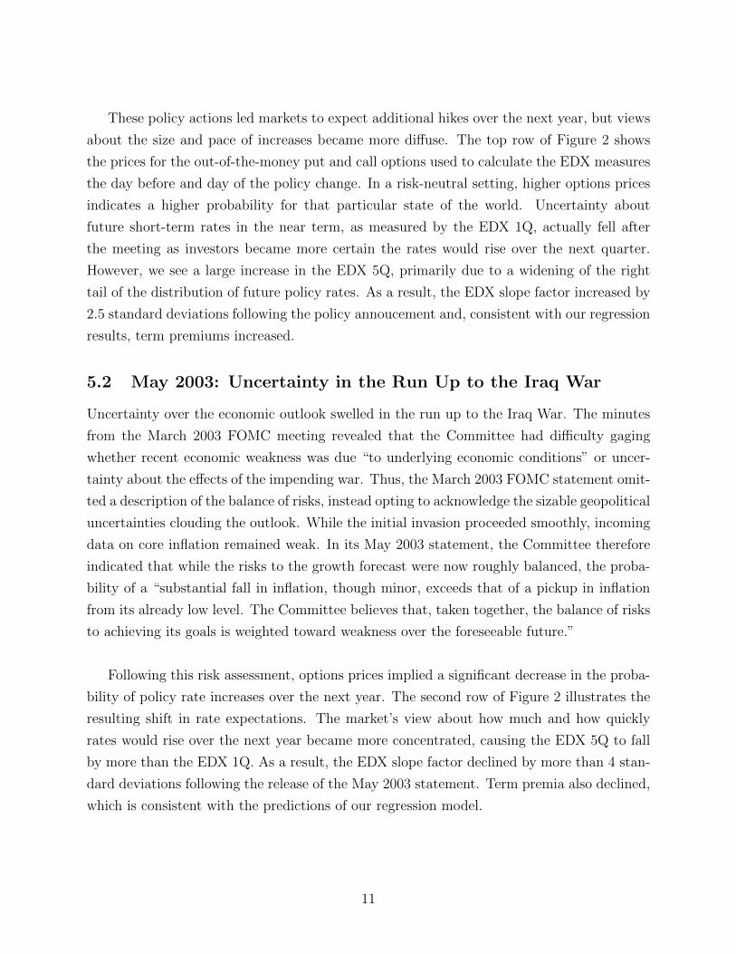
5.2 May 2003: Uncertainty in the Run Up to the Iraq War

Uncertainty over the economic outlook swelled in the run up to the Iraq War. The minutes

from the March 2003 FOMC meeting revealed that the Committee had difficulty gaging

whether recent economic weakness was due “to underlying economic conditions” or uncer-

tainty about the effects of the impending war. Thus, the March 2003 FOMC statement omit-

ted a description of the balance of risks, instead opting to acknowledge the sizable geopolitical

uncertainties clouding the outlook. While the initial invasion proceeded smoothly, incoming

data on core inflation remained weak. In its May 2003 statement, the Committee therefore

indicated that while the risks to the growth forecast were now roughly balanced, the proba-

bility of a “substantial fall in inflation, though minor, exceeds that of a pickup in inflation

from its already low level. The Committee believes that, taken together, the balance of risks

to achieving its goals is weighted toward weakness over the foreseeable future.”

Following this risk assessment, options prices implied a significant decrease in the proba-

bility of policy rate increases over the next year. The second row of Figure 2 illustrates the

resulting shift in rate expectations. The market’s view about how much and how quickly

rates would rise over the next year became more concentrated, causing the EDX 5Q to fall

by more than the EDX 1Q. As a result, the EDX slope factor declined by more than 4 stan-

dard deviations following the release of the May 2003 statement. Term premia also declined,

which is consistent with the predictions of our regression model.

11

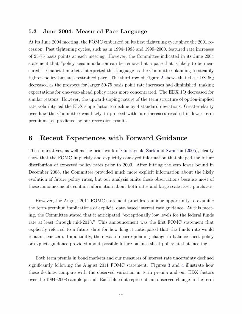
5.3 June 2004: Measured Pace Language

At its June 2004 meeting, the FOMC embarked on its first tightening cycle since the 2001 re-

cession. Past tightening cycles, such as in 1994–1995 and 1999–2000, featured rate increases

of 25-75 basis points at each meeting. However, the Committee indicated in its June 2004

statement that “policy accommodation can be removed at a pace that is likely to be mea-

sured.” Financial markets interpreted this language as the Committee planning to steadily

tighten policy but at a restrained pace. The third row of Figure 2 shows that the EDX 5Q

decreased as the prospect for larger 50-75 basis point rate increases had diminished, making

expectations for one-year-ahead policy rates more concentrated. The EDX 1Q decreased for

similar reasons. However, the upward-sloping nature of the term structure of option-implied

rate volatility led the EDX slope factor to decline by 4 standard deviations. Greater clarity

over how the Committee was likely to proceed with rate increases resulted in lower term

premiums, as predicted by our regression results.

6 Recent Experiences with Forward Guidance

These narratives, as well as the prior work of Gurkaynak, Sack and Swanson (2005), clearly

show that the FOMC implicitly and explicitly conveyed information that shaped the future

distribution of expected policy rates prior to 2009. After hitting the zero lower bound in

December 2008, the Committee provided much more explicit information about the likely

evolution of future policy rates, but our analysis omits these observations because most of

these announcements contain information about both rates and large-scale asset purchases.

However, the August 2011 FOMC statement provides a unique opportunity to examine

the term-premium implications of explicit, date-based interest rate guidance. At this meet-

ing, the Committee stated that it anticipated “exceptionally low levels for the federal funds

rate at least through mid-2013.” This announcement was the first FOMC statement that

explicitly referred to a future date for how long it anticipated that the funds rate would

remain near zero. Importantly, there was no corresponding change in balance sheet policy

or explicit guidance provided about possible future balance sheet policy at that meeting.

Both term premia in bond markets and our measures of interest rate uncertainty declined

significantly following the August 2011 FOMC statement. Figures 3 and 4 illustrate how

these declines compare with the observed variation in term premia and our EDX factors

over the 1994–2008 sample period. Each blue dot represents an observed change in the term

12

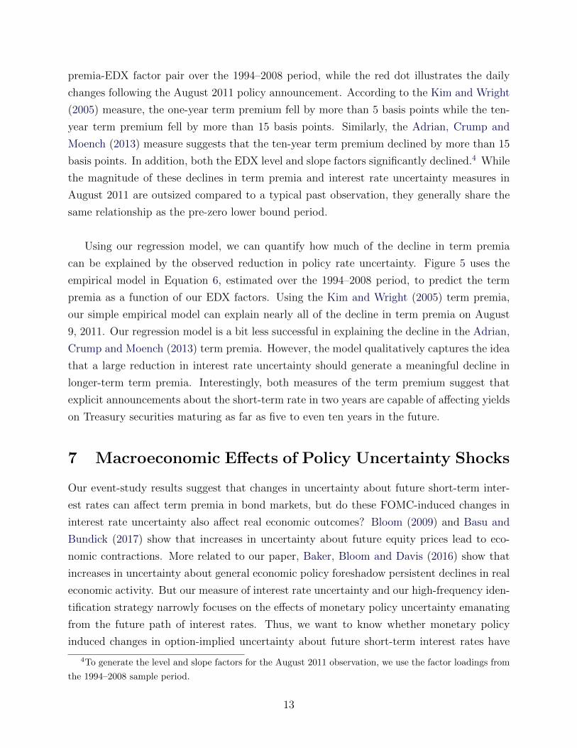
premia-EDX factor pair over the 1994–2008 period, while the red dot illustrates the daily

changes following the August 2011 policy announcement. According to the Kim and Wright

(2005) measure, the one-year term premium fell by more than 5 basis points while the ten-

year term premium fell by more than 15 basis points. Similarly, the Adrian, Crump and

Moench (2013) measure suggests that the ten-year term premium declined by more than 15

basis points. In addition, both the EDX level and slope factors significantly declined.4 While

the magnitude of these declines in term premia and interest rate uncertainty measures in

August 2011 are outsized compared to a typical past observation, they generally share the

same relationship as the pre-zero lower bound period.

Using our regression model, we can quantify how much of the decline in term premia

can be explained by the observed reduction in policy rate uncertainty. Figure 5 uses the

empirical model in Equation 6, estimated over the 1994–2008 period, to predict the term

premia as a function of our EDX factors. Using the Kim and Wright (2005) term premia,

our simple empirical model can explain nearly all of the decline in term premia on August

9, 2011. Our regression model is a bit less successful in explaining the decline in the Adrian,

Crump and Moench (2013) term premia. However, the model qualitatively captures the idea

that a large reduction in interest rate uncertainty should generate a meaningful decline in

longer-term term premia. Interestingly, both measures of the term premium suggest that

explicit announcements about the short-term rate in two years are capable of affecting yields

on Treasury securities maturing as far as five to even ten years in the future.

7 Macroeconomic Effects of Policy Uncertainty Shocks

Our event-study results suggest that changes in uncertainty about future short-term inter-

est rates can affect term premia in bond markets, but do these FOMC-induced changes in

interest rate uncertainty also affect real economic outcomes? Bloom (2009) and Basu and

Bundick (2017) show that increases in uncertainty about future equity prices lead to eco-

nomic contractions. More related to our paper, Baker, Bloom and Davis (2016) show that

increases in uncertainty about general economic policy foreshadow persistent declines in real

economic activity. But our measure of interest rate uncertainty and our high-frequency iden-

tification strategy narrowly focuses on the effects of monetary policy uncertainty emanating

from the future path of interest rates. Thus, we want to know whether monetary policy

induced changes in option-implied uncertainty about future short-term interest rates have

4To generate the level and slope factors for the August 2011 observation, we use the factor loadings from

the 1994–2008 sample period.

13

meaningful macroeconomic effects.

In the following sections, we use a structural vector autoregression (VAR) to examine

the macroeconomic effects of monetary policy induced changes in interest rate uncertainty.

Following FOMC communication that reduces the slope of the term structure of interest rate

uncertainty, we find that financial conditions ease and the economy expands. Moreover, we

find that our estimated elasticity of output with respect to the term premium is consistent

with other researchers’ findings. Overall, our VAR results suggest that monetary policy

makers may have the ability to influence economic and financial conditions through the

amount of clarity they offer about the future path of short-term interest rates.

7.1 Baseline VAR Model

To trace out the macroeconomic response to changes in interest rate uncertainty, we embed

our high-frequency slope factor into a monthly vector autoregression. To generate a monthly

series for the implied level of policy uncertainty, we follow Romer and Romer (2004) and

Barakchian and Crowe (2013) and assign a value of zero to months in which there is no

FOMC meeting and cumulatively sum the resulting slope factor series. Building on the work

of Bloom (2009), this approach is akin to putting the VIX in the VAR in levels as opposed

to first differences.

Following Romer and Romer (2004), we measure real economic activity and prices at

a monthly frequency using the natural log of both industrial production and the producer

price index for finished goods. We also include the unemployment rate in our VAR model,

which helps measure U.S. economic activity beyond factory output.5 However, our results

are unchanged if we exclude the unemployment rate from our model. Finally, we include

two financial variables: the federal funds rate and the slope of the yield curve. Including

the funds rate in our model helps control for the level of short-term interest rates at the

time of the monetary policy uncertainty shock. The slope of the yield curve is defined as the

ten-year less the one-year nominal average Treasury yield.

Following the monetary policy shock literature, we use a recursive identification scheme.

We order our policy uncertainty measure after production and prices, which maintains the

common assumption that output and prices respond to changes in monetary policy with a

5Coibion (2012) also includes the unemployment rate when measuring the real effects of monetary policy

shocks.

14

lag. However, to be consistent with our event-study evidence, we order the federal funds

rate and bond market variables after our slope factor. In Section 7.3, however, we show that

this ordering is not material for our main results. We estimate our baseline VAR model over

the 1994–2008 sample period.

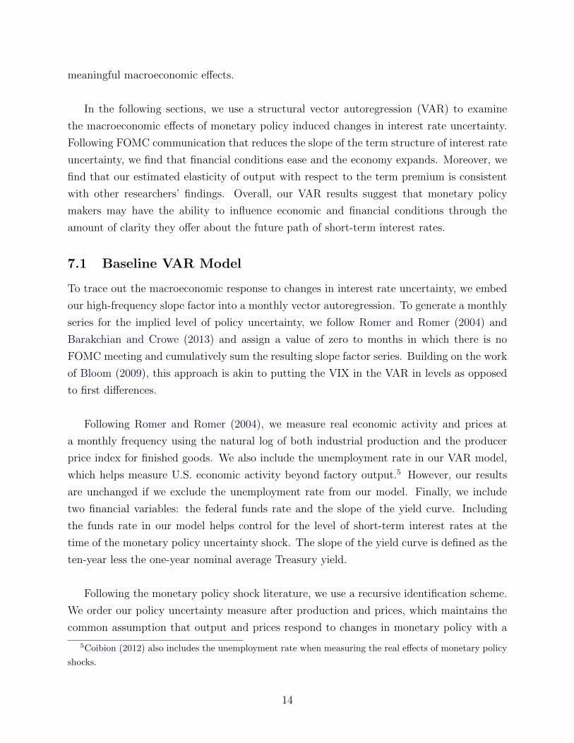
A decline in uncertainty about future monetary policy flattens the yield curve and leads

to a significant expansion of economic activity and prices. Figure 6 plots the impulse re-

sponses to a one standard deviation shock to our identified slope factor along with their

90% probability intervals calculated using a (normal) diffuse prior over the VAR parameters.

Following a typical shock, uncertainty about future short-term interest rates falls sharply at

impact and remains lower for about a year. As a result, the slope of the yield curve declines,

which is consistent with our high-frequency empirical evidence from Section 4. In addition,

the yield curve slope remains depressed for a significant period after the shock. The flatter

yield curve, a hallmark of easier financial conditions, helps stimulate production and em-

ployment. After about one year, industrial production is about 30 basis points higher and

the unemployment rate falls over 5 basis points.6 Higher levels of output lead producers to

raise prices over the next few years. The central bank endogenously responds to the increase

in output and prices by raising the federal funds rate by about 15 basis points over the next

year.

7.2 A Quantitative Comparison to Other VAR Estimates

To offer a comparison of our estimated quantitative effects with the previous literature, we

now estimate a second VAR which replaces industrial production with real GDP and re-

places the producer price index for finished goods with the consumer price index. Weale and

Wieladek (2016) use these measures of real activity and prices in their the VAR study on

the macroeconomic effects of large-scale asset purchases.7 They find that an asset purchase

announcement equal to one-percent-of-GDP has a peak effect of increasing real GDP by

0.58% and the CPI price level by 0.62%.

6Our estimated point estimate for the unemployment rate is broadly similar to the findings of Creal

and Wu (2017), who use a macro-finance term structure model to estimate the effects of interest rate

uncertainty on the macroeconomy. However, their identifying assumptions require that changes in interest-

rate uncertainty do not affect bond yields at impact, which runs counter to our high-frequency empirical

evidence in Section 4.7We obtain a measure of monthly real GDP from Macroeconomic Advisers, the same source used by

Weale and Wieladek (2016).

15

Using these estimates, along with the findings of Gagnon et al. (2011), we can com-

pute an implied elasticity of output with respect to the ten-year term premium. Gagnon

et al. (2011) find that a one-percent-of-GDP asset purchase announcement depresses the

Kim and Wright (2005) ten-year term premium by 4.4 basis points. Translating the Weale

and Wieladek (2016) estimates into an elasticity of the 10-year term premium: an asset

purchase announcement which depresses the ten-year term premium by 1 basis point leads

to an increase in real GDP of 0.13% and the CPI price level of 0.14%.

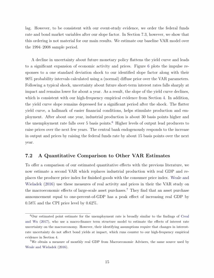
We find very similar real GDP effects compared to Weale and Wieladek (2016), but

smaller, albeit still significant, effects on the CPI price level. Figure 7 shows the impulse

responses of this alternative VAR model. A one standard deviation shock decreases the slope

factor of interest rate uncertainty by 1.4 basis points. At their peak response, real GDP

and the CPI increase by a statistically significant 0.12% and 0.05%, respectively. Using

these estimates, we can use our previous event-study results to translate our findings into

an elasticity in terms of the 10-year term premium. Table 4 shows that a 1.4 basis point

decrease in the EDX slope factor lowers the Kim and Wright (2005) 10-year term premium

by almost exactly 1 basis point. Thus, our VAR implies that a decrease in interest rate

uncertainty which depresses the ten-year term premium by 1 basis point leads to an increase

in real GDP of 0.12% and the CPI price level of 0.05%. This elasticity for real GDP is very

close the estimate of Weale and Wieladek (2016), whereas the elasticity of CPI prices is only

one third of the size of their estimate. Though taking into account the precision of the two

CPI responses, the estimates do not appear to be statistically different.

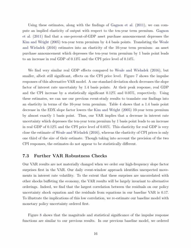
7.3 Further VAR Robustness Checks

Our VAR results are not materially changed when we order our high-frequency slope factor

surprises first in the VAR. Our daily event-window approach identifies unexpected move-

ments in interest rate volatility. To the extent that these surprises are uncorrelated with

other shocks buffeting the economy, the VAR results will be largely invariant to alternative

orderings. Indeed, we find that the largest correlation between the residuals on our policy

uncertainty shock equation and the residuals from equations in our baseline VAR is 0.17.

To illustrate the implications of this low correlation, we re-estimate our baseline model with

monetary policy uncertainty ordered first.

Figure 8 shows that the magnitude and statistical significance of the impulse response

functions are similar to our previous results. In our previous baseline model, we ordered

16

monetary policy uncertainty last, which restricts the initial response of economic activity

and prices to be zero. Importantly, Figure 8 shows that allowing industrial production and

the unemployment rate to respond on impact still results in a persistent and significant ex-

pansion in industrial production and tighter labor market conditions. This exercise addresses

Uhlig (2005)’s concern that the real effects of a monetary policy shock may hinge on the

short-run restrictions placed on these variables.

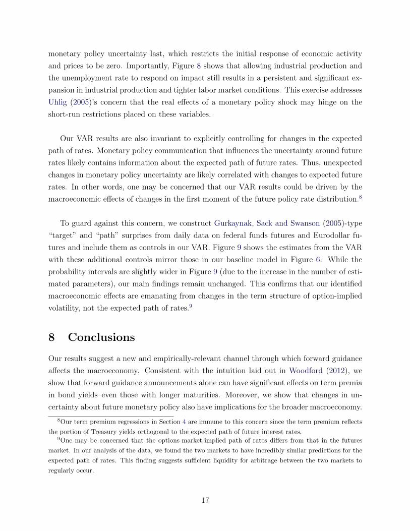
Our VAR results are also invariant to explicitly controlling for changes in the expected

path of rates. Monetary policy communication that influences the uncertainty around future

rates likely contains information about the expected path of future rates. Thus, unexpected

changes in monetary policy uncertainty are likely correlated with changes to expected future

rates. In other words, one may be concerned that our VAR results could be driven by the

macroeconomic effects of changes in the first moment of the future policy rate distribution.8

To guard against this concern, we construct Gurkaynak, Sack and Swanson (2005)-type

“target” and “path” surprises from daily data on federal funds futures and Eurodollar fu-

tures and include them as controls in our VAR. Figure 9 shows the estimates from the VAR

with these additional controls mirror those in our baseline model in Figure 6. While the

probability intervals are slightly wider in Figure 9 (due to the increase in the number of esti-

mated parameters), our main findings remain unchanged. This confirms that our identified

macroeconomic effects are emanating from changes in the term structure of option-implied

volatility, not the expected path of rates.9

8 Conclusions

Our results suggest a new and empirically-relevant channel through which forward guidance

affects the macroeconomy. Consistent with the intuition laid out in Woodford (2012), we

show that forward guidance announcements alone can have significant effects on term premia

in bond yields–even those with longer maturities. Moreover, we show that changes in un-

certainty about future monetary policy also have implications for the broader macroeconomy.

8Our term premium regressions in Section 4 are immune to this concern since the term premium reflects

the portion of Treasury yields orthogonal to the expected path of future interest rates.9One may be concerned that the options-market-implied path of rates differs from that in the futures

market. In our analysis of the data, we found the two markets to have incredibly similar predictions for the

expected path of rates. This finding suggests sufficient liquidity for arbitrage between the two markets to

regularly occur.

17

Our results also have implications for properly measuring the term-premia effects of the

FOMC’s recent large-scale asset purchases. Both forward guidance and asset purchases can

have significant effects on the term premia. During the zero lower bound period, many

FOMC announcements regarding large-scale asset purchases also contained clear communi-

cation about the future policy rates. Our results suggest that empirical models may overstate

the actual effects of asset purchases if researchers do not control for the observed changes

in interest rate uncertainty around such policy announcements. As more frequent encoun-

ters with the zero lower bound are perhaps more likely in the future, we believe that a

better understanding the individual implications for both policies remains a key focus for

policymakers.

18

References

Adrian, Tobias, Richard K. Crump, and Emanuel Moench. 2013. “Pricing the Term

Structure with Linear Regressions.” Journal of Financial Economics, 110: 110–138.

Baker, Scott R, Nicholas Bloom, and Steven J Davis. 2016. “Measuring Economic

Policy Uncertainty.” The Quarterly Journal of Economics, 131(4): 1593–1636.

Barakchian, S. Mahdi, and Christopher Crowe. 2013. “Monetary Policy Matters:

Evidence from New Shocks Data.” Journal of Monetary Economics, 60(8): 950 – 966.

Basu, Susanto, and Brent Bundick. 2017. “Uncertainty Shocks in a Model of Effective

Demand.” Econometrica, 85(3): 937–958.

Bernanke, Ben S. 2013. “Communication and Monetary Policy.” Speech on November 19,

2013.

Bloom, Nicholas. 2009. “The Impact of Uncertainty Shocks.” Econometrica, 77(3): 623–

685.

Coibion, Olivier. 2012. “Are the Effects of Monetary Policy Shocks Big or Small?” Amer-

ican Economic Journal: Macroeconomics, 4(2): 1–32.

Creal, Drew D., and Jing Cynthia Wu. 2017. “Monetary Policy Uncertainty and Eco-

nomic Fluctuations.” International Economic Review. Forthcoming.

Gagnon, Joseph, Matthew Raskin, Julie Remache, Brian Sack, et al. 2011. “The

Financial Market Effects of the Federal Reserve’s Large-Scale Asset Purchases.” Interna-

tional Journal of Central Banking, 7(1): 3–43.

Gurkaynak, Refet S, Brian Sack, and Eric Swanson. 2005. “Do Actions Speak Louder

Than Words? The Response of Asset Prices to Monetary Policy Actions and Statements.”

International Journal of Central Banking, 1(1): 55–93.

Kim, Don H., and Jonathan H. Wright. 2005. “An Arbitrage-Free Three-Factor Term

Structure Model and the Recent Behavior of Long-Term Yields and the Distant-Horizon

Forward Rates.” Working Paper.

Kuttner, Kenneth N. 2001. “Monetary Policy Surprises and Interest Rates: Evidence

from the Fed Funds Futures Market.” Journal of Monetary Economics, 47(3): 523–544.

19

Romer, Christina D., and David H. Romer. 2004. “A New Measure of Monetary

Shocks: Derivation and Implications.” American Economic Review, 94(4): 1055–1084.

Rudebusch, Glenn D., and Eric T. Swanson. 2012. “The Bond Premium in a DSGE

Model with Long-Run Real and Nominal Risks.” American Economic Journal: Macroe-

conomics, 4(1): 105–143.

Uhlig, Harald. 2005. “What are the Effects of Monetary Policy on Output? Results from

an Agnostic Identification Procedure.” Journal of Monetary Economics, 52(2): 381–419.

Weale, Martin, and Tomasz Wieladek. 2016. “What are the Macroeconomic Effects of

Asset Purchases?” Journal of Monetary Economics, 79: 81–93.

Woodford, Michael. 2012. “Methods of Policy Accommodation at the Interest-Rate Lower

Bound.” The Changing Policy Landscape: 2012 Jackson Hole Symposium.

20

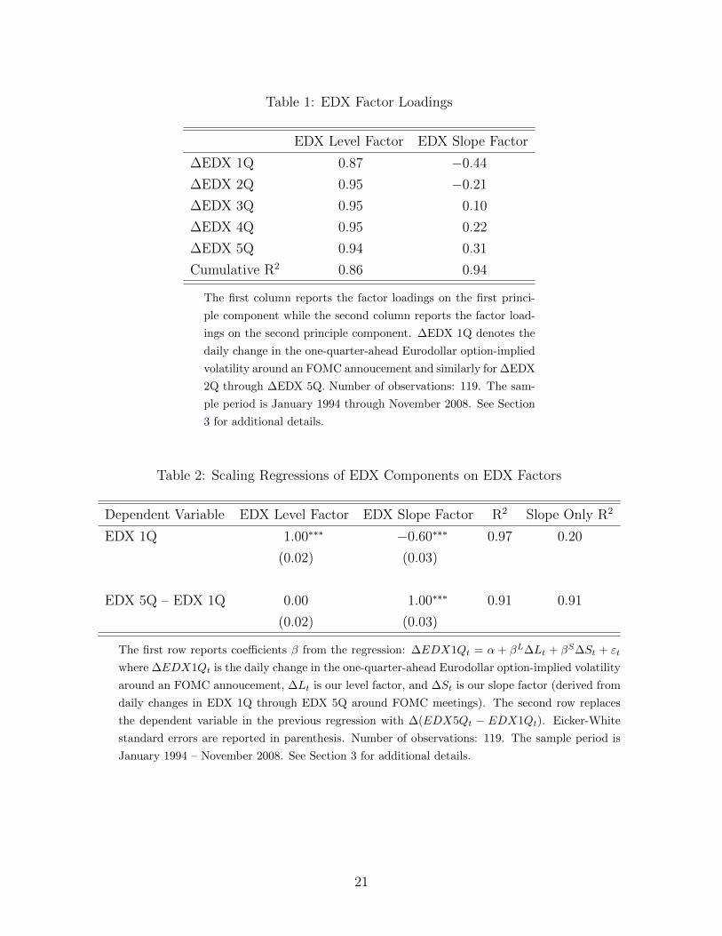
Table 1: EDX Factor Loadings

EDX Level Factor EDX Slope Factor

∆EDX 1Q 0.87 −0.44

∆EDX 2Q 0.95 −0.21

∆EDX 3Q 0.95 0.10

∆EDX 4Q 0.95 0.22

∆EDX 5Q 0.94 0.31

Cumulative R2 0.86 0.94

The first column reports the factor loadings on the first princi-

ple component while the second column reports the factor load-

ings on the second principle component. ∆EDX 1Q denotes the

daily change in the one-quarter-ahead Eurodollar option-implied

volatility around an FOMC annoucement and similarly for ∆EDX

2Q through ∆EDX 5Q. Number of observations: 119. The sam-

ple period is January 1994 through November 2008. See Section

3 for additional details.

Table 2: Scaling Regressions of EDX Components on EDX Factors

Dependent Variable EDX Level Factor EDX Slope Factor R2 Slope Only R2

EDX 1Q 1.00∗∗∗ −0.60∗∗∗ 0.97 0.20

(0.02) (0.03)

EDX 5Q – EDX 1Q 0.00 1.00∗∗∗ 0.91 0.91

(0.02) (0.03)

The first row reports coefficients β from the regression: ∆EDX1Qt = α + βL∆Lt + βS∆St + εt

where ∆EDX1Qt is the daily change in the one-quarter-ahead Eurodollar option-implied volatility

around an FOMC annoucement, ∆Lt is our level factor, and ∆St is our slope factor (derived from

daily changes in EDX 1Q through EDX 5Q around FOMC meetings). The second row replaces

the dependent variable in the previous regression with ∆(EDX5Qt − EDX1Qt). Eicker-White

standard errors are reported in parenthesis. Number of observations: 119. The sample period is

January 1994 – November 2008. See Section 3 for additional details.

21

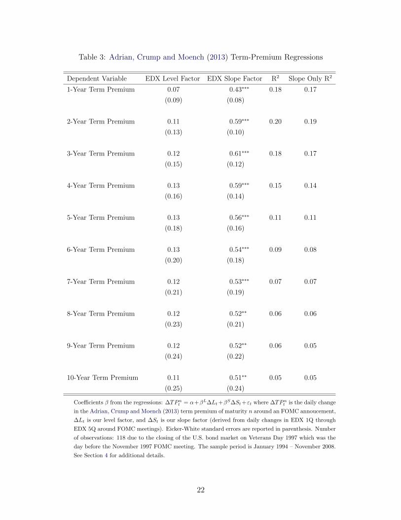
Table 3: Adrian, Crump and Moench (2013) Term-Premium Regressions


1-Year Term Premium 0.07 0.43∗∗∗ 0.18 0.17

(0.09) (0.08)


(0.13) (0.10)


(0.15) (0.12)


(0.16) (0.14)


(0.18) (0.16)


(0.20) (0.18)


(0.21) (0.19)

8-Year Term Premium 0.12 0.52∗∗ 0.06 0.06

(0.23) (0.21)


(0.24) (0.22)


(0.25) (0.24)

Coefficients β from the regressions: ∆TPnt = α+βL∆Lt +βS∆St +εt where ∆TPn

t is the daily change

in the Adrian, Crump and Moench (2013) term premium of maturity n around an FOMC annoucement,

∆Lt is our level factor, and ∆St is our slope factor (derived from daily changes in EDX 1Q through

EDX 5Q around FOMC meetings). Eicker-White standard errors are reported in parenthesis. Number

of observations: 118 due to the closing of the U.S. bond market on Veterans Day 1997 which was the

day before the November 1997 FOMC meeting. The sample period is January 1994 – November 2008.

See Section 4 for additional details.

22

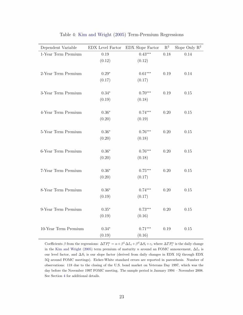
Table 4: Kim and Wright (2005) Term-Premium Regressions



(0.12) (0.12)

2-Year Term Premium 0.29∗ 0.61∗∗∗ 0.19 0.14

(0.17) (0.17)


(0.19) (0.18)


(0.20) (0.19)


(0.20) (0.18)


(0.20) (0.18)


(0.20) (0.17)


(0.19) (0.17)


(0.19) (0.16)


(0.19) (0.16)

Coefficients β from the regressions: ∆TPnt = α+βL∆Lt +βS∆St +εt where ∆TPn

t is the daily change

in the Kim and Wright (2005) term premium of maturity n around an FOMC annoucement, ∆Lt is

our level factor, and ∆St is our slope factor (derived from daily changes in EDX 1Q through EDX

5Q around FOMC meetings). Eicker-White standard errors are reported in parenthesis. Number of

observations: 118 due to the closing of the U.S. bond market on Veterans Day 1997, which was the

day before the November 1997 FOMC meeting. The sample period is January 1994 – November 2008.


23

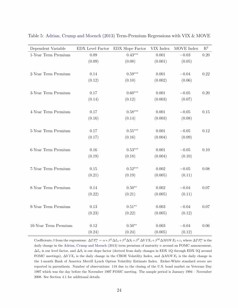
Table 5: Adrian, Crump and Moench (2013) Term-Premium Regressions with VIX & MOVE

Dependent Variable EDX Level Factor EDX Slope Factor VIX Index MOVE Index R2

1-Year Term Premium 0.09 0.43∗∗∗ 0.001 −0.03 0.20

(0.09) (0.08) (0.001) (0.05)


(0.12) (0.10) (0.002) (0.06)


(0.14) (0.12) (0.003) (0.07)


(0.16) (0.14) (0.003) (0.08)


(0.17) (0.16) (0.004) (0.09)


(0.19) (0.18) (0.004) (0.10)


(0.21) (0.19) (0.005) (0.11)

8-Year Term Premium 0.14 0.50∗∗ 0.002 −0.04 0.07

(0.22) (0.21) (0.005) (0.11)


(0.23) (0.22) (0.005) (0.12)


(0.24) (0.24) (0.005) (0.12)

Coefficients β from the regressions: ∆TPnt = α+βL∆Lt+β

S∆St+βV ∆V IXt+β

M∆MOV Et+εt where ∆TPnt is the

daily change in the Adrian, Crump and Moench (2013) term premium of maturity n around an FOMC annoucement,

∆Lt is our level factor, and ∆St is our slope factor (derived from daily changes in EDX 1Q through EDX 5Q around

FOMC meetings), ∆V IXt is the daily change in the CBOE Volatility Index, and ∆MOV Et is the daily change in

the 1-month Bank of America Merrill Lynch Option Volatility Estimate Index. Eicker-White standard errors are

reported in parenthesis. Number of observations: 118 due to the closing of the U.S. bond market on Veterans Day

1997 which was the day before the November 1997 FOMC meeting. The sample period is January 1994 – November

2008. See Section 4.1 for additional details.

24

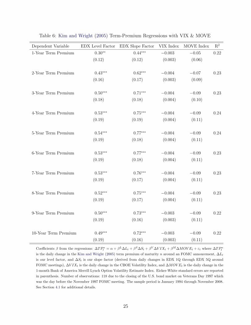
Table 6: Kim and Wright (2005) Term-Premium Regressions with VIX & MOVE

Dependent Variable EDX Level Factor EDX Slope Factor VIX Index MOVE Index R2

1-Year Term Premium 0.30∗∗ 0.44∗∗∗ −0.003 −0.05 0.22

(0.12) (0.12) (0.003) (0.06)

2-Year Term Premium 0.43∗∗∗ 0.62∗∗∗ −0.004 −0.07 0.23

(0.16) (0.17) (0.003) (0.09)


(0.18) (0.18) (0.004) (0.10)


(0.19) (0.19) (0.004) (0.11)


(0.19) (0.18) (0.004) (0.11)


(0.19) (0.18) (0.004) (0.11)


(0.19) (0.17) (0.004) (0.11)


(0.19) (0.17) (0.004) (0.11)


(0.19) (0.16) (0.003) (0.11)


(0.19) (0.16) (0.003) (0.11)

Coefficients β from the regressions: ∆TPnt = α + βL∆Lt + βS∆St + βV ∆V IXt + βM∆MOV Et + εt where ∆TPn

t

is the daily change in the Kim and Wright (2005) term premium of maturity n around an FOMC annoucement, ∆Lt

is our level factor, and ∆St is our slope factor (derived from daily changes in EDX 1Q through EDX 5Q around

FOMC meetings), ∆V IXt is the daily change in the CBOE Volatility Index, and ∆MOV Et is the daily change in the

1-month Bank of America Merrill Lynch Option Volatility Estimate Index. Eicker-White standard errors are reported

in parenthesis. Number of observations: 118 due to the closing of the U.S. bond market on Veterans Day 1997 which

was the day before the November 1997 FOMC meeting. The sample period is January 1994 through November 2008.

See Section 4.1 for additional details.

25

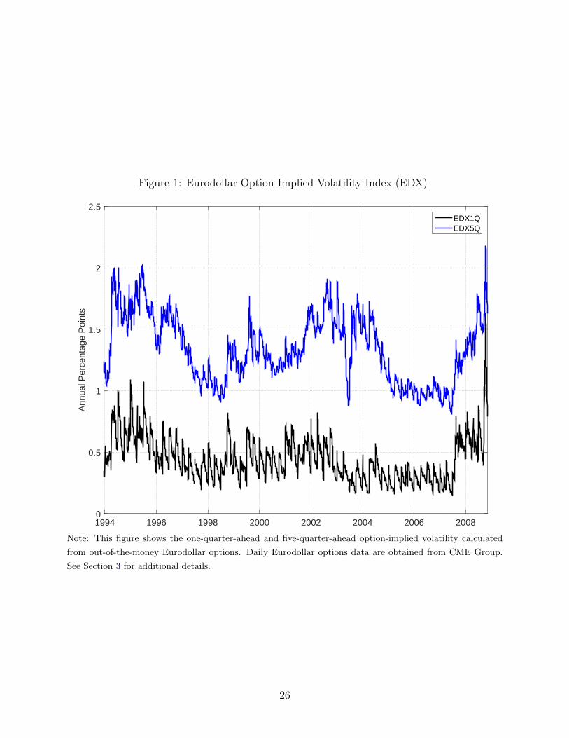
Figure 1: Eurodollar Option-Implied Volatility Index (EDX)

1994 1996 1998 2000 2002 2004 2006 2008

Ann

ual P

erce

ntag

e P

oint

s

0

0.5

1

1.5

2

2.5EDX1QEDX5Q

Note: This figure shows the one-quarter-ahead and five-quarter-ahead option-implied volatility calculated

from out-of-the-money Eurodollar options. Daily Eurodollar options data are obtained from CME Group.


26

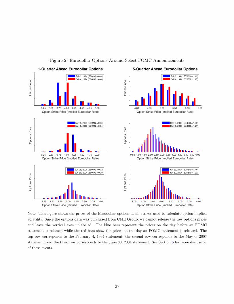
Figure 2: Eurodollar Options Around Select FOMC Announcements

3.25 3.50 3.75 4.00 4.25 4.50 4.75 5.00Option Strike Price (Implied Eurodollar Rate)

Opt

ions

Pric

e

1-Quarter Ahead Eurodollar OptionsFeb 3, 1994 (EDX1Q = 0.48)Feb 4, 1994 (EDX1Q = 0.46)

4.00 4.50 5.00 5.50 6.00 6.50Option Strike Price (Implied Eurodollar Rate)

Opt

ions

Pric

e

5-Quarter Ahead Eurodollar OptionsFeb 3, 1994 (EDX5Q = 1.13)Feb 4, 1994 (EDX5Q = 1.17)


Opt

ions

Pric

e

May 5, 2003 (EDX1Q = 0.36)May 6, 2003 (EDX1Q = 0.34)

0.50 1.00 1.50 2.00 2.50 3.00 3.50 4.00 4.50 5.00 5.50 6.00Option Strike Price (Implied Eurodollar Rate)

O

ptio

ns P

rice

May 5, 2003 (EDX5Q = 1.35)May 6, 2003 (EDX5Q = 1.27)


Opt

ions

Pric

e

Jun 29, 2004 (EDX1Q = 0.32)Jun 30, 2004 (EDX1Q = 0.29)


Opt

ions

Pric

e

Jun 29, 2004 (EDX5Q = 1.40)Jun 30, 2004 (EDX5Q = 1.32)

Note: This figure shows the prices of the Eurodollar options at all strikes used to calculate option-implied

volatility. Since the options data was purchased from CME Group, we cannot release the raw options prices

and leave the vertical axes unlabeled. The blue bars represent the prices on the day before an FOMC

statement is released while the red bars show the prices on the day an FOMC statement is released. The

top row corresponds to the February 4, 1994 statement; the second row corresponds to the May 6, 2003

statement; and the third row corresponds to the June 30, 2004 statement. See Section 5 for more discussion

of these events.

27

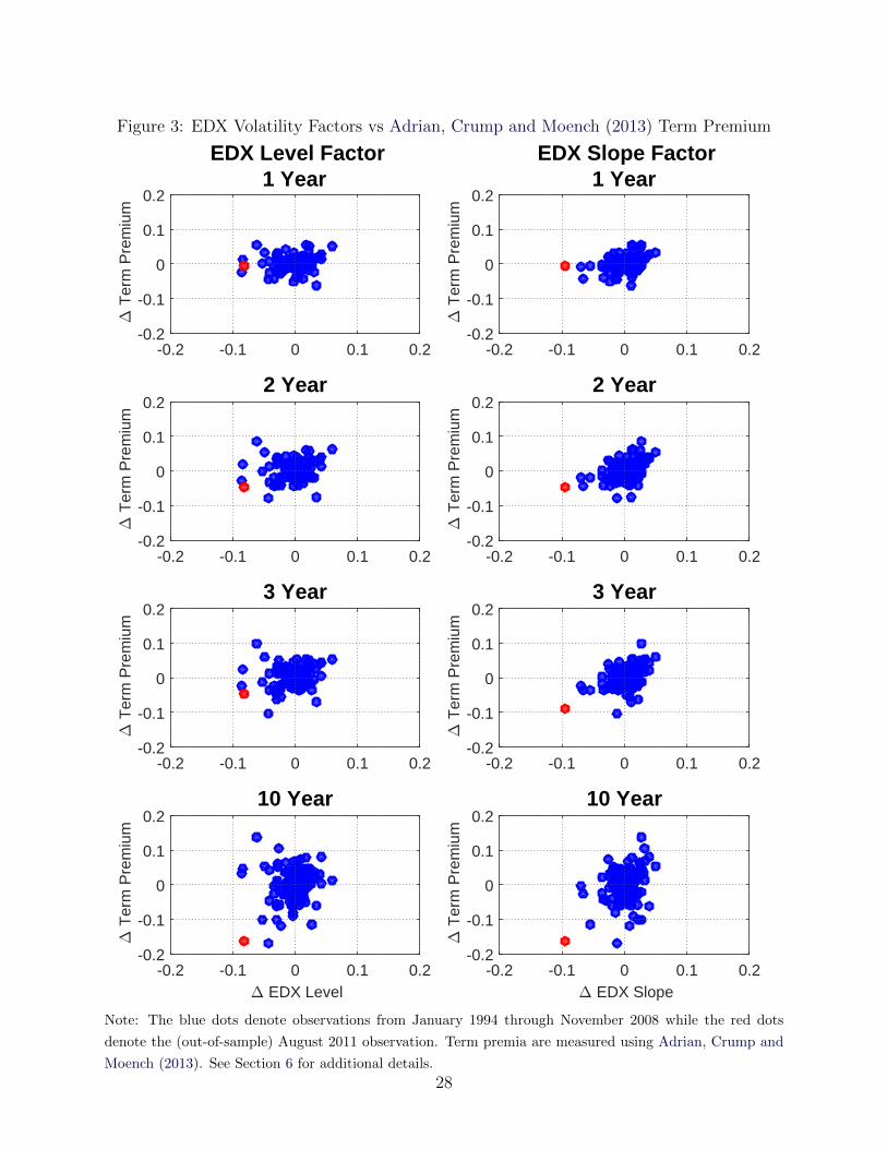
Figure 3: EDX Volatility Factors vs Adrian, Crump and Moench (2013) Term Premium

EDX Level Factor1 Year

-0.2 -0.1 0 0.1 0.2

" T

erm

Pre

miu

m

-0.2

-0.1

0

0.1

0.2

2 Year

-0.2 -0.1 0 0.1 0.2

" T

erm

Pre

miu

m

-0.2

-0.1

0

0.1

0.2

3 Year

-0.2 -0.1 0 0.1 0.2

" T

erm

Pre

miu

m

-0.2

-0.1

0

0.1

0.2

10 Year

" EDX Level-0.2 -0.1 0 0.1 0.2

" T

erm

Pre

miu

m

-0.2

-0.1

0

0.1

0.2

EDX Slope Factor1 Year

-0.2 -0.1 0 0.1 0.2

" T

erm

Pre

miu

m

-0.2

-0.1

0

0.1

0.2

2 Year

-0.2 -0.1 0 0.1 0.2

" T

erm

Pre

miu

m

-0.2

-0.1

0

0.1

0.2

3 Year

-0.2 -0.1 0 0.1 0.2

" T

erm

Pre

miu

m

-0.2

-0.1

0

0.1

0.2

10 Year

" EDX Slope-0.2 -0.1 0 0.1 0.2

" T

erm

Pre

miu

m

-0.2

-0.1

0

0.1

0.2

Note: The blue dots denote observations from January 1994 through November 2008 while the red dots

denote the (out-of-sample) August 2011 observation. Term premia are measured using Adrian, Crump and

Moench (2013). See Section 6 for additional details.

28

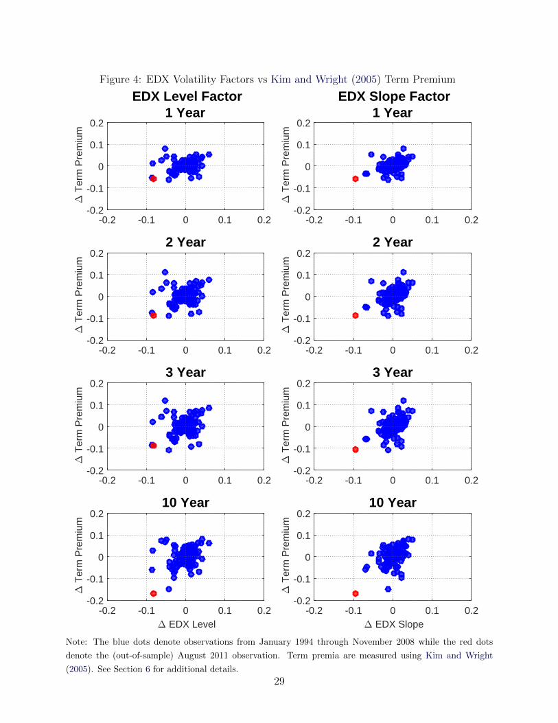
Figure 4: EDX Volatility Factors vs Kim and Wright (2005) Term Premium

EDX Level Factor1 Year

-0.2 -0.1 0 0.1 0.2

" T

erm

Pre

miu

m

-0.2

-0.1

0

0.1

0.2

2 Year

-0.2 -0.1 0 0.1 0.2

" T

erm

Pre

miu

m

-0.2

-0.1

0

0.1

0.2

3 Year

-0.2 -0.1 0 0.1 0.2

" T

erm

Pre

miu

m

-0.2

-0.1

0

0.1

0.2

10 Year

" EDX Level-0.2 -0.1 0 0.1 0.2

" T

erm

Pre

miu

m

-0.2

-0.1

0

0.1

0.2

EDX Slope Factor1 Year

-0.2 -0.1 0 0.1 0.2

" T

erm

Pre

miu

m

-0.2

-0.1

0

0.1

0.2

2 Year

-0.2 -0.1 0 0.1 0.2

" T

erm

Pre

miu

m

-0.2

-0.1

0

0.1

0.2

3 Year

-0.2 -0.1 0 0.1 0.2

" T

erm

Pre

miu

m

-0.2

-0.1

0

0.1

0.2

10 Year

" EDX Slope-0.2 -0.1 0 0.1 0.2

" T

erm

Pre

miu

m

-0.2

-0.1

0

0.1

0.2

Note: The blue dots denote observations from January 1994 through November 2008 while the red dots

denote the (out-of-sample) August 2011 observation. Term premia are measured using Kim and Wright

(2005). See Section 6 for additional details.

29

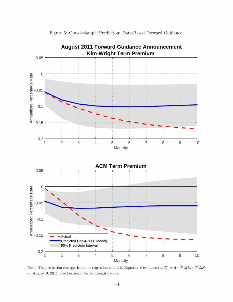
Figure 5: Out-of-Sample Prediction: Date-Based Forward Guidance

ACM Term Premium

Maturity1 2 3 4 5 6 7 8 9 10

Ann

ualiz

ed P

erce

ntag

e R

ate

-0.2

-0.15

-0.1

-0.05

0

0.05

ActualPredicted (1994-2008 Model)90% Prediction Interval

August 2011 Forward Guidance AnnouncementKim-Wright Term Premium

Maturity1 2 3 4 5 6 7 8 9 10

Ann

ualiz

ed P

erce

ntag

e R

ate

-0.2

-0.15

-0.1

-0.05

0

0.05

Note: The prediction emerges from our regression model in Equation 6 evaluated at Tnt = α+βL∆Lt+β

S∆St

on August 9, 2011. See Section 6 for additional details.

30

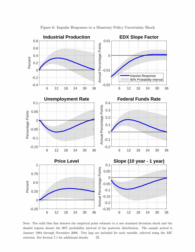
Figure 6: Impulse Responses to a Monetary Policy Uncertainty Shock

Industrial Production

6 12 18 24 30 36

Per

cent

-0.4

-0.2

0

0.2

0.4

0.6

0.8

Unemployment Rate

6 12 18 24 30 36

Per

cent

age

Poi

nts

-0.15

-0.1

-0.05

0

0.05

0.1

Price Level

6 12 18 24 30 36

Per

cent

-0.25

0

0.25

0.5

0.75

1

EDX Slope Factor

6 12 18 24 30 36

Ann

ual P

erce

ntag

e P

oint

s

-0.02

-0.01

0

0.01

Impulse Response90% Probability Interval

Federal Funds Rate

6 12 18 24 30 36

Ann

ual P

erce

ntag

e P

oint

s

-0.2

-0.1

0

0.1

0.2

0.3

0.4

Slope (10 year - 1 year)

6 12 18 24 30 36

Ann

ual P

erce

ntag

e P

oint

s

-0.25

-0.2

-0.15

-0.1

-0.05

0

0.05

0.1

Note: The solid blue line denotes the empirical point estimate to a one standard deviation shock and the

shaded regions denote the 90% probability interval of the posterior distribution. The sample period is

January 1994 through November 2008. Two lags are included for each variable, selected using the AIC

criterion. See Section 7.1 for additional details. 31

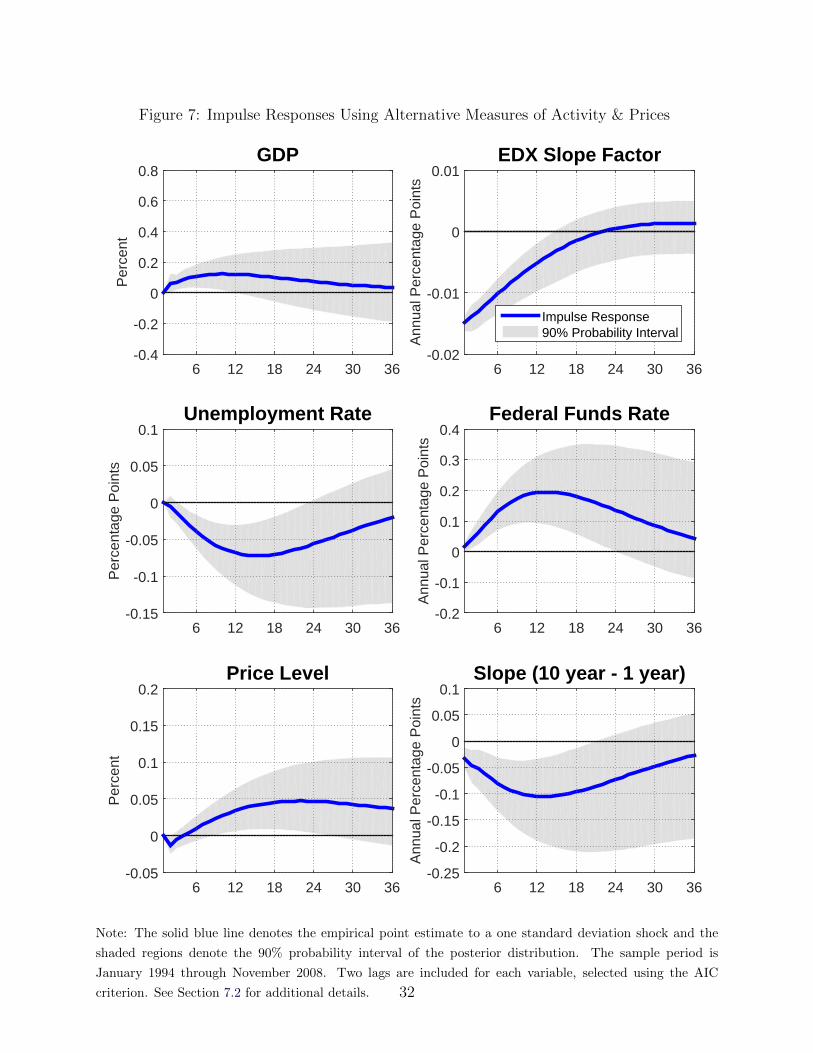
Figure 7: Impulse Responses Using Alternative Measures of Activity & Prices

GDP

6 12 18 24 30 36

Per

cent

-0.4

-0.2

0

0.2

0.4

0.6

0.8

Unemployment Rate

6 12 18 24 30 36

Per

cent

age

Poi

nts

-0.15

-0.1

-0.05

0

0.05

0.1

Price Level

6 12 18 24 30 36

Per

cent

-0.05

0

0.05

0.1

0.15

0.2

EDX Slope Factor

6 12 18 24 30 36

Ann

ual P

erce

ntag

e P

oint

s

-0.02

-0.01

0

0.01


Federal Funds Rate

6 12 18 24 30 36

Ann

ual P

erce

ntag

e P

oint

s

-0.2

-0.1

0

0.1

0.2

0.3

0.4


6 12 18 24 30 36

Ann

ual P

erce

ntag

e P

oint

s

-0.25

-0.2

-0.15

-0.1

-0.05

0

0.05

0.1





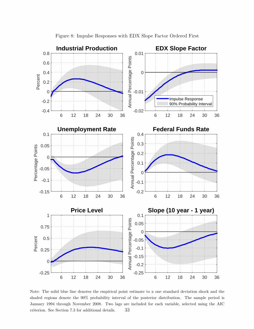
Figure 8: Impulse Responses with EDX Slope Factor Ordered First


6 12 18 24 30 36

Per

cent

-0.4

-0.2

0

0.2

0.4

0.6

0.8

Unemployment Rate

6 12 18 24 30 36

Per

cent

age

Poi

nts

-0.15

-0.1

-0.05

0

0.05

0.1

Price Level

6 12 18 24 30 36

Per

cent

-0.25

0

0.25

0.5

0.75

1

EDX Slope Factor

6 12 18 24 30 36

Ann

ual P

erce

ntag

e P

oint

s

-0.02

-0.01

0

0.01


Federal Funds Rate

6 12 18 24 30 36

Ann

ual P

erce

ntag

e P

oint

s

-0.2

-0.1

0

0.1

0.2

0.3

0.4


6 12 18 24 30 36

Ann

ual P

erce

ntag

e P

oint

s

-0.25

-0.2

-0.15

-0.1

-0.05

0

0.05

0.1





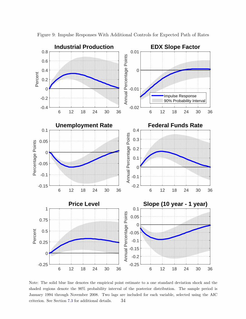
Figure 9: Impulse Responses With Additional Controls for Expected Path of Rates


6 12 18 24 30 36

Per

cent

-0.4

-0.2

0

0.2

0.4

0.6

0.8

Unemployment Rate

6 12 18 24 30 36

Per

cent

age

Poi

nts

-0.15

-0.1

-0.05

0

0.05

0.1

Price Level

6 12 18 24 30 36

Per

cent

-0.25

0

0.25

0.5

0.75

1

EDX Slope Factor

6 12 18 24 30 36

Ann

ual P

erce

ntag

e P

oint

s

-0.02

-0.01

0

0.01


Federal Funds Rate

6 12 18 24 30 36

Ann

ual P

erce

ntag

e P

oint

s

-0.2

-0.1

0

0.1

0.2

0.3

0.4


6 12 18 24 30 36

Ann

ual P

erce

ntag

e P

oint

s

-0.25

-0.2

-0.15

-0.1

-0.05

0

0.05

0.1





Forward Guidance, Monetary Policy Uncertainty, and …...Forward Guidance, Monetary Policy...

Documents

Transcript of Forward Guidance, Monetary Policy Uncertainty, and …...Forward Guidance, Monetary Policy...