Formulae and Software for Particular Solutions to the ...appelo/preprints/part_sol_manuscript.pdfat...

INTERNATIONAL JOURNAL FOR NUMERICAL AND ANALYTICAL METHODS IN GEOMECHANICSInt. J. Numer. Anal. Meth. Geomech. 2016; 00:1–19Published online in Wiley InterScience (www.interscience.wiley.com). DOI: 10.1002/nag

Formulae and Software for Particular Solutions to the ElasticWave Equation in Curved Geometries

Kristoffer Virta∗and Daniel Appelo†

Division of Scientific Computing, Department of Information Technology, Uppsala University, Box 337, 75105 Uppsala,Sweden. Department of Mathematics and Statistics, University of New Mexico, 1 University of New Mexico,

Albuquerque, NM 87131.

SUMMARY

We present formulae for particular solutions to the elastic wave equation in cylindrical geometries. Weconsider scattering and diffraction from a cylinder and inclusion and surface waves exterior and interior to acylindrical boundary. The solutions are used to compare two modern numerical methods for the elastic waveequation. Associated to this paper is the free software PeWe that implements the exact solutions. Copyrightc© 2016 John Wiley & Sons, Ltd.

Received . . .

KEY WORDS: Elastic wave equation; exact solutions; curved geometries; scattering and diffraction;surface waves; SBP-SAT; discontinuous Galerkin method

1. INTRODUCTION

Pressure and shear waves associated with seismic events in the Earth as well as waves in plates,

beams and solid structures are governed by the elastic wave equation. The domain in which the

waves are traveling is in general of finite extension in at least one spatial direction and may contain

material heterogeneities. This introduces conditions at the boundaries of the domain and at interfaces

between differing materials that a solution must satisfy. Two frequently occurring conditions are the

vanishing of stress at a boundary and the continuity of displacement and stress at a material interface.

The former appears for example at the surface of the Earth and the later at internal interfaces due

to its layered structure. A distinguishing characteristic of the interaction between elastic waves and

boundaries or interfaces is that mode conversion occurs. That is, when a wave, either pressure or

shear, impinges on a boundary or interface it is converted into both shear and pressure waves upon

reflection. Disturbances at boundaries or interfaces may generate a wave that clings to the boundary

or interface and travels independent of the pressure and shear waves. In general domains boundaries

and interfaces are non-planar. A curved geometry has a radius of curvature which introduces a length

scale that may differ from that of the scales represented by the present wavelengths, this gives rise to

dispersion and possibly attenuation in solutions. A planar boundary or interface does not have this

feature. The effect of curvature, existence of boundary and interface waves and mode conversion

at boundaries and interfaces account for the relative complexity of wave motion in elastic solids

compared to similar problems in acoustics.

†Supported in part by NSF Grant DMS-1319054. Any conclusions or recommendations expressed in this paper are thoseof the author and do not necessarily reflect the views NSF.∗Correspondence to: Division of Scientific Computing, Department of Information Technology, Uppsala University, Box337, 75105 Uppsala, Sweden.

Copyright c© 2016 John Wiley & Sons, Ltd.

Prepared using nagauth.cls [Version: 2010/05/13 v2.00]

2

The complexity of elastic wave propagation makes a numerical solution of the elastic wave

equation appealing and a lot of research is devoted to the design of stable, accurate and efficient

methods. Preferably a numerical method should be able to handle complex geometries as well as

boundary and interface conditions. To ascertain the quality and correctness of a numerical solution

a comparison with a known solution should be performed. The known solution can be found in

some different ways. For example, the known solution can be constructed by the manufactured

solution technique where a function, e.g. a trigonometric polynomial, is chosen and inserted into

the equation. As the function does not satisfy the equation, boundary and interior forcing are added

so that the function is instead a solution to a modified, forced problem. This method verifies that the

numerical scheme is stable and accurate. A manufactured solution is however unphysical and does

not test the capability of the numerical method to handle the various physical phenomena that arise

at boundaries and interfaces.

Another approach is to use a reference solution as the known solution. Now, a numerical solution

with given data is computed using a computational grid with a small discretization length. This

solution is considered exact and comparisons are made with numerical solutions computed on

coarser grids. This method is unappealing, for every set of data a solution that requires substantial

computational power and time is needed and, regardless of the resolution of the reference solution,

it is still only an approximate solution. In addition the use of a reference solution does not eliminate

the possibility that the discretized equations may not be the same as the equations one set out to

solve in the first place.

A third approach to constructing known solutions is to solve the equations exactly by separation

of variables techniques. When the domain of interest contains planar boundaries or interfaces, time-

harmonic exact solutions to the elastic wave equation that exhibits typical boundary or interface

behavior are easily obtained using plane wave analysis [12]. Also, boundary value problems

involving transient time behavior have been studied. The archetype being Lamb’s problem first

introduced by Lamb, [17], in which the boundary of an elastic half-plane is being subjected to a

transient load in the direction normal to the surface. Exact solutions to variations of Lamb’s problem

have been presented by Mooney [21] and latter used to evaluate the performance of a numerical

methods in [23]. Exact solutions to problems involving internal sources in three dimensional,

layered media was used by Day et.al., [11] to give a systematic comparison of the performance

of different numerical codes that solve the elastic wave equation.

In recent years a number of new methods for the elastic wave equation has been presented

[29, 3, 13, 18, 1, 9, 8, 15, 25] however there has been a dearth in open source software providing

exact solutions that can be used for validating the correctness and benchmarking the performance

of old and new methods. In the context of seismology the notable exceptions is the monograph

by Kausel [14], the suite EX2DDIR/EX2DELEL/EX2DVAEL by Berg et al. [5] and the program

Gar6more 2D/3D by Diaz and Ezziani, [7]. The latter two methods rely on the Cagniard-de-Hoop

technique and are restricted to planar / layered geometries including point sources. Nowadays

most of the numerical methods are capable to handle curved geometries and we therefore focus

here on developing exact solutions and software for the homogenous (un-forced) equations in

cylindrical geometries with free boundaries and internal interfaces. Our hope is that these solutions

and associated software, feely available from [28], will augment existing open source software.

Solutions representing surface waves at the convex boundary of a circular cylinder was first

investigated by Sezawa [24]. Sezawa showed how the effect of curvature enter into the dispersion

relations. The solutions where described in terms of Bessel functions of the first kind, for this reason

a numerical solution in the general case requires availability of numerical values of Bessel functions

of the first kind with sufficient accuracy for an arbitrary argument. A qualitative diagram that

illustrates the dispersive nature of the surface wave was given by Sezawa for the case λ = µ, where

λ is Lame’s first parameter and µ is the shear modulus, but no numerical values where presented.

The change in nature of surface waves on the concave boundary of a circular cylinder in that the

wave is now attenuated was discussed by Epstein [10]. The dispersion relation governing the phase

velocity now involves Hankel functions of complex order, which was remarked by Epstein to make

computations more involved. In this paper we circumvent this difficulty by instead expressing the

Copyright c© 2016 John Wiley & Sons, Ltd. Int. J. Numer. Anal. Meth. Geomech. (2016)Prepared using nagauth.cls DOI: 10.1002/nag

3

solutions in terms of Hankel functions of integer order but with a complex argument which makes

it easier to find roots of the corresponding dispersion relation using numerical methods.

Exact solutions that represent scattering by a spherical cavity or inclusion resulting from an

incident plane pressure wave have been constructed by Pao and Mow [22]. The incoming, scattered

and diffracted waves were represented by Fourier series expansions, with coefficients determined to

fulfill the boundary or interface conditions at the surface of the sphere. This approach was also used

by Miles [20] to study a plane pressure or shear wave impinging on a rigid circular cylindrical body,

here the boundary conditions at the cylinder differ from the ones mentioned above.

The goal of this paper is to make available to computational scientists exact solutions to the elastic

wave equation that represent physical phenomena occurring at boundaries and interfaces in curved

geometries. These exact solutions are presented in terms of formulas that can be evaluated, using

supplied software (freely available), to generate initial and boundary data. The supplied routines can

also be used to compute of errors in the numerical solution at any given time and point in space.

In this paper we present the solutions to four different problems:

• Scattering by a circular cylindrical cavity in an elastic medium,

• Scattering and diffraction by a circular cylindrical inclusion in an elastic medium,

• Surface waves on the convex boundary of an elastic circular cylinder,

• Surface waves on the concave boundary of a circular cylindrical cavity in an elastic medium.

The derivation of solutions representing the first two cases is inspired by [22] in that the same

technique is used but here the scatterer is an infinite circular cylinder, thus reducing the number

of relevant spatial dimensions to two. The derivation of solutions representing the last two cases

follows the work of Sezawa [24] and Epstein [10] but complementing these works with numerical

parameters necessary to use these particular solutions in actual numerical computations. Numerical

values of the present parameters are presented in B. As an illustration of the usage of the particular

solutions, we present numerical results using two methods. The first method is based on finite

differences, the second method is based on the discontinuous Galerkin method. The finite difference

method requires a structured grid while the discontinuous Galerkin method handles unstructured

grids. For ease of comparison we use the same grids for both methods in our computations, the

construction of the grids are described in detail to facilitate future computations with other methods.

2. THE ELASTIC WAVE EQUATION IN CYLINDRICAL GEOMETRIES

Consider a circular cylinder enclosed in an infinite surrounding medium. The radius of the cylinder

is a > 0 and its axis is parallel to one of the coordinate axes, say z. We consider the case when the

material properties of the cylinder and the surrounding medium are different and we allow for either

to be a vacuum. The displacement in the direction of the cylindrical axis is omitted, the remaining

radial and azimuthal components of the displacement, p(r, θ, t) and q(r, θ, t), are functions of the

cylindrical coordinates, r and θ and can be expressed as

p = φr +1

rψθ,

q =1

rφθ − ψr,

(1)

where φ and ψ solve the wave equations

ρφtt = c2p

(

1

rφr + φrr +

1

r2φθθ

)

, (2)

ρψtt = c2s

(

1

rψr + ψrr +

1

r2ψθθ

)

. (3)

Here

cp =

√

λ+ 2µ

ρ, cs =

√

µ

ρ, (4)


4

ρ is the density of the elastic medium, λ is Lames first parameter and µ is the shear modulus. The

functions φ and ψ represent pressure and shear waves propagating with phase velocities cp and cs,

respectively. In Cartesian coordinates x = r cos(θ) and y = r sin(θ) and the horizontal and vertical

displacement components u(x, y, t) and v(x, y, t) are given by

u(x, y, t) = cos(θ)p(r, θ, t) − sin(θ)q(r, θ, t),

v(x, y, t) = sin(θ)p(r, θ, t) + cos(θ)q(r, θ, t).(5)

If the surrounding media or the cylinder is a vacuum no wave motion occurs in the vacuum and

the surface of the cylinder is free of traction. This is described by the boundary conditions

λ

(

pr(a, θ, t) +1

rqθ(a, θ, t) +

1

rp(a, θ, t)

)

+ 2µpr(a, θ, t) = 0,

µ

(

1

rpθ(a, θ, t) + qr(a, θ, t)−

1

rq(a, θ, t)

)

= 0.

(6)

When there is no vacuum the normal and tangential components of the displacement and stress

tensor are required to be continuous across the interface, r = a, between the two materials. Let the

quantities inside the cylinder be denoted with a prime, then the interface conditions take the form

p(a, θ, t) = p′(a, θ, t),

q(a, θ, t) = q′(a, θ, t),

(λ+ 2µ)pr(a, θ, t) +λ

a(qθ(a, θ, t) + p(a, θ, t)) =

(λ′ + 2µ′)p′r(a, θ, t) +µ′

a(q′θ(a, θ, t) + p′(a, θ, t)),

µ (pθ(a, θ, t) + aqr(a, θ, t)− q(a, θ, t)) =

µ′ (p′θ(a, θ, t) + aq′r(a, θ, t)− q′(a, θ, t)) .

(7)

3. PARTICULAR SOLUTIONS TO THE ELASTIC WAVE EQUATION

In this section two types of of particular solutions to the elastic wave equation are derived. The first

type describes the scattering of an incident pressure wave striking a cylindrical cavity or inclusion.

In the first case the interior of the cylinder is a vacuum and its boundary is free of traction. In the

second case the interior of the cylinder is of a material differing from the surrounding medium and

continuity of displacements as well as tractions are required at the boundary of the cylinder. The

second type of solutions relates to waves propagated on the surface of the cylinder. In this case a

distinction is made between waves traveling on the convex boundary of the interior of the cylinder,

the surrounding media being a vacuum, or the concave exterior of the cylinder, its interior being a

vacuum.

3.1. Scattering and Diffraction of Pressure Waves by a Cylindrical Cavity or Inclusion

Consider an incident time-harmonic plane compressional wave

φ(i)(r, θ, t) = φ0ei(ωt−γpr cos(θ)), φ0 = constant, (8)

traveling in the direction θ = 0. When the wave strikes the cylindrical cavity or inclusion mode

conversion occurs, i.e., the reflections will consist of both pressure waves φ(s) and shear waves

ψ(s). In the case of an inclusion the diffracted waves will also consist of pressure and shear waves,

φ′(d) and ψ′(d) respectively. The total incident and reflected displacement fields in r > a are given

by (1) as

p = φ(i)r + φ(s)r +1

rψ(s)θ ,

q =1

r

(

φ(i)θ + φ

(s)θ

)

− ψ(s)r .

(9)


5

The total diffracted displacement fields inside the inclusion, r < a, are given by

p′ = φ′(d)r +1

rψ′(d)θ ,

q′ =1

rφ′(d)θ − ψ′(d)

r .

(10)

The incident wave automatically solves equation (2) when γp = ω/cp.

Since the wave equation is separable in cylindrical coordinates the ansatz

φ(s) = RΘeiωt, (11)

separates equation (2) into

d2

dθ2Θ+ k2Θ = 0,

d2

dr2R+

1

r+

(

γ2p − k2

r2

)

R = 0.

(12)

The solutions to (12) are

Θ = A cos(kθ) +B sin(kθ), (13)

R = CH(1)k (γpr) +DH

(2)k (γpr), (14)

where H(1)k and H

(2)k are Hankel functions of the first and second kind, respectively. Symmetry

with respect to the x-axis requires B = 0 in (13) and requiring that Θ be single-valued (Θ(θ) =Θ(θ + 2π)) indicates that k is an integer say k = n.

For large values of the argument the Hankel functions have the asymptotic expansions

H(1)n (z) ≈

(

2

πz

)1/2

ei(z−π4− kaπ

2 ) (1− . . . ) , (15)

H(2)n (z) ≈

(

2

πz

)1/2

e−i(z−π4− kaπ

2 ) (1 + . . . ) . (16)

Since the time dependence is eiωt an outward propagating wave must have the form ei(ωt−γpr) so

taking C = 0 in (14) is appropriate for the present case. The scattered pressure wave field is thus

given by a superposition of solutions of the form (11)

φ(s)(r, θ, t) = eiωt∞∑

n=0

AnH(2)n (γpr) cos(nθ), r > a. (17)

By the same reasoning the scattered shear wave field may be written

ψ(s)(r, θ, t) = eiωt∞∑

n=0

BnH(2)n (γsr) sin(nθ), r > a, (18)

where γs = ω/cs.

The diffracted wave fields are defined inside the cylindrical inclusion and are required to

be bounded at the origin. For this reason the Hankel function in the expression (14) for the

corresponding R is replaced by the Bessel function of the first kind. The resulting solutions inside

r < a are written as

φ′(d)(r, θ, t) = eiωt∞∑

n=0

CnJn(γ′pr) cos(nθ),

ψ′(d)(r, θ, t) = eiωt∞∑

n=0

DnJn(γ′sr) sin(nθ),

(19)


6

where quantities with primes relate to those defined inside the cylindrical inclusion. To match

expressions term by term we write the incident wave φ(i) in Bessel functions of the first kind using

the identity

e−iγpr cos(θ) =

∞∑

n=0

(ǫn(−i)nJn(γpr) cos(nθ)) , (20)

where{

ǫ0 = 1,ǫn = 2, n ≥ 1.

By (9) the radial and azimuthal components, representing the incident and scattered fields in r > a,

are given by

p(r, θ, t) = eiωt∞∑

n=0

(

φ0ǫn(−i)nd

drJn(γpr)

+And

drH(2)

n (γpr) +Bnn

rH(2)

n (γsr)

)

cos(nθ),

q(r, θ, t) = eiωt∞∑

n=0

(−nrφ0ǫn(−i)nJn(γpr)

+An−nrH(2)

n (γpr) −Bnd

drH(2)

n (γsr)

)

sin(nθ).

(21)

Solutions that represent the diffracted fields in r < a are given via (10) by

p′(r, θ, t) =eiωt∞∑

n=0

(

Cnd

drJn(γ

′pr) +Dn

n

rJn(γ

′sr)

)

cos(nθ),

q′(r, θ, t) =eiωt∞∑

n=0

(

Cn−nrH(2)

n (γ′pr) −Dnd

drJn(γ

′sr)

)

sin(nθ).

(22)

In the case of a cylindrical cavity no wave motion occurs inside the cylinder and Cn = Dn = 0 in

(22). The coefficients An and Bn of (21) are determined by substituting the solutions (21) into the

boundary conditions (6) and equating coefficients of cosnθ and sinnθ in virtue of Fourier’s method.

This results in the linear systems

[

m(11)n m

(12)n

m(21)n m

(22)n

]

[

An

Bn

]

= φ0ǫn(−i)n+1

[

f(1)n

f(2)n

]

, n = 1, 2, . . . , (23)

for the coefficientsAn andBn. Exact expressions for arbitrary values of ρ, λ and µ of the coefficients

m(ij)n and f

(i)n , i = 1, 2, j = 1, 2, n = 1, 2, . . . , are presented in A.

Similarly, inserting the solutions (21)-(22) into the interface conditions (7) and equating

coefficients of cosnθ and sinnθ results in the linear systems

m(11)n m

(12)n m

(13)n m

(14)n

m(21)n m

(22)n m

(23)n m

(24)n

m(31)n m

(32)n m

(33)n m

(34)n

m(41)n m

(42)n m

(43)n m

(44)n

An

Bn

Cn

Dn

= φ0ǫn(−i)n+1

f (1)

f(2)n

f(3)n

f(4)n

, n = 1, 2, . . . , (24)

for the coefficients An, Bn, Cn, Dn. Exact expressions for arbitrary values of ρ, λ and µ of the

coefficients m(ij)n and f

(i)n , i = 1, 4, j = 1, 4, n = 1, 2, . . . , are presented in A.

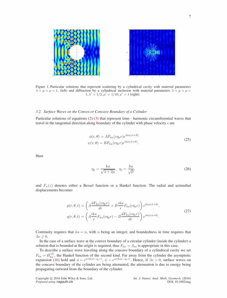
Figure 1 displays the magnitude of the displacement field given by the solutions (21)-(22). Here

the series have been truncated when the coefficients An, Bn, Cn, Dn are smaller than roundoff.


7

Figure 1. Particular solutions that represent scattering by a cylindrical cavity with material parametersλ = µ = ρ = 1, (left) and diffraction by a cylindrical inclusion with material parameters λ = µ = ρ =

1, λ′ = 1/2, µ′= 1/10, ρ′ = 1 (right).

3.2. Surface Waves on the Convex or Concave Boundary of a Cylinder

Particular solutions of equations (2)-(3) that represent time - harmonic circumferential waves that

travel in the tangential direction along boundary of the cylinder with phase velocity c are

φ(r, θ) = AFka(cηpr)eika(ct+θ)

ψ(r, θ) = BFka(cηsr)eika(ct+θ).

(25)

Here

ηp =ka√λ+ 2µ

, ηs =ka√µ, (26)

and Fn(z) denotes either a Bessel function or a Hankel function. The radial and azimuthal

displacements becomes

p(r, θ, t) =

(

AdFka(cηpr)

dr+B

ika

rFka(cηsr)

)

eika(ct+θ),

q(r, θ, t) =

(

Aika

rFka(cηpr) −B

dFka(cηsr)

dr

)

eika(ct+θ).

(27)

Continuity requires that ka = n, with n being an integer, and boundedness in time requires that

ℑc ≥ 0.

In the case of a surface wave at the convex boundary of a circular cylinder (inside the cylinder) a

solution that is bounded at the origin is required, thus Fka = Jka is appropriate in this case.

To describe a surface wave traveling along the concave boundary of a cylindrical cavity we set

Fka = H(2)ka , the Hankel function of the second kind. Far away from the cylinder the asymptotic

expansion (16) hold and φ ∼ eic(kat−ηpr), ψ ∼ eic(kat−ηsr). Hence, if ℑc > 0, surface waves on

the concave boundary of the cylinder are being attenuated, the attenuation is due to energy being

propagating outward from the boundary of the cylinder.


8

Figure 2. Particular solutions that represent surface waves at the convex (left) or concave boundary of acylinder (right). In both figures the material parameters are λ = µ = ρ = 1.

Inserting the solutions (27) into the boundary conditions (6) at r = a results in the following

homogeneous system of equations with unknowns A and B,

−µ(

c2(

η2s − 2η2p)

Fka (cηpa)− 2d2Fka (cηpa)

dr2

)

A

+2µik

(

dFka (cηsa)

dr− Fka (cηsa)

a

)

B = 0, (28)

2µik

(

dFka (cηpa)

dr− Fka (cηpa)

a

)

A

+µ

(

(

c2η2s − 2k2)

Fka (cηsa) +2

a

dFka (cηsa)

dr

)

B = 0. (29)

A solution exists if and only if there is a phase velocity c such that the determinant of the system

(28)-(29)

D(c) =−1

µ2

(

c2(

η2s − 2η2p)

Fka (cηpa)− 2d2Fka (cηpa)

dr2

)

×(

(

c2η2s − 2k2)

Fka (cηsa) +2

a

dFka (cηsa)

dr

)

− 4k2(

dFka (cηpa)

dr− Fka (cηpa)

a

)(

dFka (cηsa)

dr− Fka (cηsa)

a

)

,

(30)

vanishes. Note that unlike the Rayleigh wave at a planar boundary, the surface wave on a curved

boundary is dispersive, i.e. the phase velocity c = c(k) depends on the wave number k.

3.3. Computing Phase Velocities

Explicit usage of the expressions (27) requires knowledge of the location of a zero c of the

determinant (30). Surface waves on the convex or concave boundary of the cylinder are represented

by taking Fka = Jka or Fka = H(2)ka in (30), respectively. In both cases it is required that ka is an

integer in order for the solution to be single-valued. The Bessel function of the first kind Jka is real

valued for real arguments when the order is an integer but the Hankel function of the second kind

H(2)ka may have a non-negative imaginary part for any argument. For this reason real zeros of the

determinant (30) are sought when considering surface waves on a convex boundary and complex-

valued zeros with ℑc > 0 are sought when considering surface waves on a concave boundary.

Numerical methods was used to find zeros with 16 digits accuracy. In both cases the zeros are

seen to be non-unique. That is, for for each wave number a multitude of phase velocities exists.

Tables II and III displays some computed values of c for both cases.


9

4. NUMERICAL METHODS AND GRID GENERATION

This section briefly presents the numerical methods used and gives a detailed description of the

grids used in the computations. The detailed description of the grids used should facilitate future

comparison with other numerical methods.

As mentioned in the introduction the solutions we use here are freely available in the open source

software PeWe which can obtained at [28]. Examples of how PeWe can be used in Matlab and

Fortran programs are also given at [28].

4.1. The Finite-Difference Method

The finite-difference method used in the following experiments was developed by Duru et.al., [8, 9].

It is based on discretizing the elastic wave equation in two spatial dimensions written as the second

order system

utt = µ∆u+ (λ+ µ)(ux + vy)x,vtt = µ∆v + (λ+ µ)(ux + vy)y,

(31)

where u and v are the vertical and horizontal displacement components, respectively. The spatial

discretization uses high order finite difference operators that satisfies a summation-by-parts (SBP)

rule [26, 19]. Boundary and interface conditions are imposed weakly via the simultaneous-

approximation-term (SAT) method [6]. With the SBP-SAT methodology the local order of accuracy

at a grid point in the interior of the computational domain is in general 2p, where p is an integer.

In the vicinity of a boundary or interface the order of accuracy decreases to p. When discretizing

a second-order hyperbolic system with the SBP-SAT methodology it can be shown, [27], that the

global order of accuracy is p+ 2. The finite difference method used in this paper has p = 3, resulting

in a fifth order accurate method.

4.2. The Discontinuous Galerkin Method

The discontinuous Galerkin method, described in detail in [2], is designed to mimic the dynamics

of the elastic energy of the system. The method discretizes the the first order system (in time)

ut = u,vt = v,ut = µ∆u + (λ+ µ)(ux + vy)x,vt = µ∆v + (λ+ µ)(ux + vy)y,

(32)

by a variational formulation where the first two equations are tested against the variational derivative

of the potential energy density

G =λ

2

(

∂u

∂x+∂v

∂y

)2

+2µ

2

(

(

∂u

∂x

)2

+

(

∂v

∂y

)2

+1

2

(

∂u

∂y+∂v

∂x

)2)

. (33)

The formulation in [2] allows for both energy conserving fluxes and fluxes of upwind type, here we

exclusively use the upwind-type. Further the formulation in [2] allows for different approximations

spaces for the displacement and velocity. Here we choose both the approximation spaces to be

tensor product polynomials of degree q which, when used together with the upwind flux, results in

a method that is of order q + 1 in space. For the evolution in time we use the classic fourth order

accurate Runge-Kutta method. An open source implementation of the discontinuous Galerkin solver

can be obained from [4].

4.3. Grid Generation

The particular solutions presented in this paper are defined on three different two-dimensional

domains,

• D1: the interior of a cylinder of radius a,


10

• D2: the exterior of a cylinder of radius a,

• D3: a whole elastic plane with a cylindrical inclusion of a differing material and radius a.

Here we present a description of how the grids used in the following experiments are constructed.

Examples of the grids can be found in Figure 3.

The domains are handled by decomposing each domain in a multi-block fashion. The domain D1

is split into five blocks and the domain D2 is split into four. The domain D3 is discretized by a grid

consisting of the union of the grids discretizing D1 and D2.

To this end, let (ξ, η) ∈ [0, 1]2 = S be the coordinates of the unit square. All blocks Bi have four

boundaries defined by parametrized curves

CiS = (xiS(ξ), yiS(ξ)) , CiN = (xiN (ξ), yiN (ξ)) ,

CiW = (xiW (η), yiW (η)) , CiE = (xiE(η), yiE(η)) ,

where CiS and CiN describe one pair of opposing sides and CiW and CiE the other pair. Let PiSW

denote the point of intersection between the curves CiS and CiW , then a bijection (x, y) = Ti(ξ, η)from S to Bi is given by the transfinite interpolation

Ti(ξ, η) = (1− η)CiS + ηCiN + (1 − ξ)CiW + ξCiE− ξηPiNE − ξ(1− η)PiSE − η(1 − ξ)PiNW − (1 − ξ)(1− η)PiSW .

The unit square S is discretized by the points

ξj = jhξ, hξ = 1/(Niξ − 1), j = 0, . . . , Niξ − 1,

ηk = khη, hη = 1/(Niη − 1), k = 0, . . . , Niη − 1,(34)

where Niξ and Niη are integers determining the number of grid points in the spatial directions of

the discretization of the block Bi. The corresponding grid points are computed as

(xj , yk) = Ti(ξj , ηk). (35)

We now give details on how each of the domains D1 −D3 are discretized. D1 is decomposed into

five blocks B(1)1 - B(1)

5 . The block B(1)1 is a square at the center of the cylinder with corners at the

points (±ad,±ad), where a is the radius of the cylinder and 0 < d < 1. Its bounding curves are

C(1)1S = a (2dξ − d,−d) ,

C(1)1N = a (2dξ − d, d) ,

C(1)1W = a (−d, 2dη − d) ,

C(1)1E = a (d, 2dη − d) ,

(36)

The block B(1)2 is defined by its bounding curves,

C(1)2S = C(1)

1N ,

C(1)2N = a

(

ξ√2−

√

1/2,

√

1−(

ξ√2−

√

1/2)2)

,

C(1)2W = a (−η(1− d)− d, η(1 − d) + d) ,

C(1)2E = a (η(1− d) + d, η(1 − d) + d) .

(37)

The bounding curves of the remaining blocks B(1)3 - B(1)

5 that constitute D1 are obtained via

C(1)ij = C(1)

i−1j

[

cosπ/2 cosπ/2sinπ/2 − sinπ/2

]

, i = 3, 4, 5, j = S,N,W,E. (38)


11

D2 represents a cylindrical cavity in an infinite surrounding media and needs to be truncated in

numerical computations. We construct the computational grid such that the cavity of radius a is

centered inside a square of side 2D. In this way D2 consists of four blocks B(2)1 - B(2)

4 . The bounding

curves of the block B(2)1 are given by

C(1)2S = a

(

ξ√2− 1/

√2,

√

1− (ξ√2− 1/

√2)2)

,

C(1)2N = (D, 2Dξ −D) ,

C(1)2W =

(

−η(D − a/√2)− a/

√2, η(D − a/

√2) + a/

√2)

,

C(1)2E =

(

η(D − a/√2) + a/

√2, η(D − a/

√2) + a/

√2)

,

(39)

The bounding curves of the remaining blocks B(2)2 - B(2)

4 that constitute D2 are obtained via rotation

by a factor π/2 as in (38).

The domain D3 consists of the union of the nine blocks that constitutes D1 and D2. Figure 3

illustrates the grids used in this paper.

-2 0 2-3

-2

-1

0

1

2

3

-2 0 2-3

-2

-1

0

1

2

3

-2 0 2-3

-2

-1

0

1

2

3

Figure 3. Structure of the grids used to discretize D1,D2 and D3.

Remark 1

We note that the grids we use are not optimal and that it might be possible to obtain better results

for the discontinuous Galerkin methods with an unstructured grid. The reason for using these block-

structured grids is that it is easier to compare the results from different, structured and unstructured,

methods.

5. NUMERICAL EXPERIMENTS

The particular solutions presented above provide non-trivial test problems for numerical methods

that solve the elastic wave equation. The solutions were chosen to carefully test how well a

numerical method can handle the boundary and interface conditions in the presence of a curved

geometry.

Let Unum(tk) and Uexact(tk) be the numerical and the exact solution at time tk. We define the

relative maximum and L2 errors

emax(tk) =‖Unum(tk)−U

exact(tk)‖∞max0≤t≤T

‖Uexact(t)‖∞, (40)

e2(tk) =‖Unum(tk)−U

exact(tk)‖2‖Uexact(0)‖2

. (41)

Note that the maximum norm is made relative by the max norm in space and over the computational

time. To approximate the maximum norm we compute the maximum over discrete points on the


12

grids, for the finite difference method these points are the grid points and for the discontinuous

Galerkin method we sample the solution in a suitable number of (equidistant in (ξ, η)) points on

each element. For the finite difference method the L2 norm is approximated by a simple Riemann

sum and for the discontinuous Galerkin method we use the Gaussian quadrature used to compute

the elements of the mass and stiffness matrices.

5.1. Scattering of a Plane Wave

In this example we compute solutions to the plane wave scattering problem with the exterior solution

(21) and, in the case of an inclusion, the interior solution (22).

In both cases the radius of the cylinder a is taken to be one, the frequency in time ω, entering

(21)-(22) through the factor eiωt, is set to 4π, and the material parameters outside the cylinder are

set to λ = µ = ρ = 1. For the case of an inclusion the material parameters inside the cylinder are

λ′ = 1/2, µ′ = 1/10 and ρ′ = 1. The temporal period is 2π/ω = 1/2 and we solve the equations for

10 periods, i.e. until time 5. Initial data for this experiment is constructed by truncating the infinite

series when the coefficients are zero to machine precision.

50 100 15010-6

10-5

10-4

10-3

10-2

10-1

100

#DOFpBpD

dG-3

dG-5

dG-7

dG-9

FD

e 2(5)

50 100 15010-6

10-5

10-4

10-3

10-2

10-1

100

#DOFpBpD

dG-3

dG-5

dG-7

dG-9

FD

e max(5)

Figure 4. The cavity experiment. The discrete L2 and maximum error for the discontinuous Galerkinmethods and the finite difference method. The horizontal axis is displaying the number of degrees of freedom

per block per dimension.

5.1.1. Results for the Cylindrical Cavity The cavity is centered inside the square [−3, 3]× [−3, 3](this corresponds to setting D = 3 in (39)). At the boundaries of the square the exact solution

is imposed at all times and at the boundary of the cylinder a traction free boundary condition is

imposed. Detailed descriptions how the boundary conditions are imposed for the two methods can

be found in the references [2, 9, 8].

The computational grid is composed of the blocks B(i)2 , i = 1 . . . 4 discretized by Niξ = Niη =

N points. To compare the finite difference method with discontinuous Galerkin methods using

polynomials of degrees q = 3, 5, 7, 9 we compute solutions for a sequence of refined grids. In Figure

4 we report the maximum and L2 errors for the different methods as a function of the number of

degrees of freedom per block and per dimension, #DOFpBpD. For the finite difference method this

is simply N and for the discontinuous Galerkin methods this is N × (q + 1).The errors measured in the L2 norm for the finite difference method and the dG method with

q = 5 are almost identical. For the dG method with q = 3 the errors are bigger and for q = 7 and

q = 9 they are smaller as expected. The observed rate of the convergence of the finite difference

method is 6.00.

When the errors are measured in the maximum norm the finite difference method outperforms

the dG method with q = 3 and q = 5 while the results obtained with the dG method with q = 7 and

q = 9 are still better than those obtained with the finite difference method. Overall, the convergence

behavior of the finite difference method appears to be more robust than for the dG method. The

observed rate of the convergence of the finite difference method is 5.47.


13

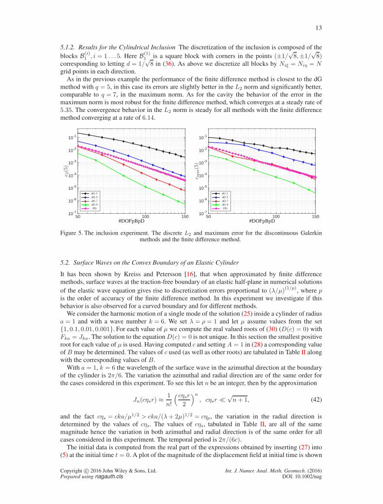
5.1.2. Results for the Cylindrical Inclusion The discretization of the inclusion is composed of the

blocks B(i)1 , i = 1 . . . 5. Here B(1)

1 is a square block with corners in the points (±1/√8,±1/

√8)

corresponding to letting d = 1/√8 in (36). As above we discretize all blocks by Niξ = Niη = N

grid points in each direction.

As in the previous example the performance of the finite difference method is closest to the dG

method with q = 5, in this case its errors are slightly better in the L2 norm and significantly better,

comparable to q = 7, in the maximum norm. As for the cavity the behavior of the error in the

maximum norm is most robust for the finite difference method, which converges at a steady rate of

5.35. The convergence behavior in the L2 norm is steady for all methods with the finite difference

method converging at a rate of 6.14.

50 100 15010-7

10-6

10-5

10-4

10-3

10-2

10-1

#DOFpBpD

dG-3

dG-5

dG-7

dG-9

FD

e 2(5)

50 100 15010-7

10-6

10-5

10-4

10-3

10-2

10-1

#DOFpBpD

dG-3

dG-5

dG-7

dG-9

FD

e max(5)

Figure 5. The inclusion experiment. The discrete L2 and maximum error for the discontinuous Galerkinmethods and the finite difference method.

5.2. Surface Waves on the Convex Boundary of an Elastic Cylinder

It has been shown by Kreiss and Petersson [16], that when approximated by finite difference

methods, surface waves at the traction-free boundary of an elastic half-plane in numerical solutions

of the elastic wave equation gives rise to discretization errors proportional to (λ/µ)(1/p), where pis the order of accuracy of the finite difference method. In this experiment we investigate if this

behavior is also observed for a curved boundary and for different methods.

We consider the harmonic motion of a single mode of the solution (25) inside a cylinder of radius

a = 1 and with a wave number k = 6. We set λ = ρ = 1 and let µ assume values from the set

{1, 0.1, 0.01, 0.001}. For each value of µ we compute the real valued roots of (30) (D(c) = 0) with

Fka = Jka. The solution to the equationD(c) = 0 is not unique. In this section the smallest positive

root for each value of µ is used. Having computed c and settingA = 1 in (28) a corresponding value

ofB may be determined. The values of c used (as well as other roots) are tabulated in Table II along

with the corresponding values of B.

With a = 1, k = 6 the wavelength of the surface wave in the azimuthal direction at the boundary

of the cylinder is 2π/6. The variation the azimuthal and radial direction are of the same order for

the cases considered in this experiment. To see this let n be an integer, then by the approximation

Jn(cηsr) ≈1

n!

(cηsr

2

)n

, cηsr ≪√n+ 1, (42)

and the fact cηs = cka/µ1/2 > cka/(λ+ 2µ)1/2 = cηp, the variation in the radial direction is

determined by the values of cηs. The values of cηs, tabulated in Table II, are all of the same

magnitude hence the variation in both azimuthal and radial direction is of the same order for all

cases considered in this experiment. The temporal period is 2π/(6c).The initial data is computed from the real part of the expressions obtained by inserting (27) into

(5) at the initial time t = 0. A plot of the magnitude of the displacement field at initial time is shown


14

in Figure 2. The numerical solution is propagated for 6 temporal periods, after this time the waves

has traversed the cylinder in the circumferential direction exactly once.

0 1 2 3 4 5 6

10-3

10-2

10-1

100

µ = 1

µ = 0.1

µ = 0.01

µ = 0.001

# Periods

e max(t)

0 1 2 3 4 5 6

10-3

10-2

10-1

100

µ = 1

µ = 0.1

µ = 0.01

µ = 0.001

# Periods

e max(t)

Figure 6. The maximum error as a function of time for a sequence of smaller values of µ using a fixedresolution of the surface wave, finite difference solution to the left and discontinuous Galerkin solution to

the right.

5.2.1. Results The computational grid is composed of the blocks B(1)i , i = 1, . . . , 5. We let the the

square block B(1)1 have its corners at the points (±1/

√8,±1/

√8) by taking d = 1/

√8 in (36)

and (37). For the finite difference method B(1)1 is discretized with N1ξ = N1η = 30 points and

B(1)i , i = 2, . . . , 5 is discretized with N2ξ = 30, N2η = 16 grid points in each spatial direction. This

yields a grid with 2820 degrees of freedom. This results in a grid that has the same grid spacing

along the Cartesian coordinate axis and is conforming to the grid B(1)1 . This grid corresponds to 20

grid points per wavelength in the azimuthal direction at the boundary of the cylinder and a resolution

of about 30 grid points in the radial direction.

For the dG method we choose q = 5 and discretize all five blocks by 4× 4 grids, i.e. we use

5× 44 × 62 = 2880 degrees of freedom.

The time-step used with the finite difference method is chosen as in [9] and is approximately

∆t = 4.9× 10−4, while the time step in the dG method is ∼ 2.4× 10−3 for µ = 1 and increasing

to ∼ 4.2× 10−3 for µ = 0.001.

Figure 6 displays the maximum error as a function of time. For the finite difference method the

error is about 2 magnitudes larger for µ = 0.001 compared to µ = 1 even though the wave is equally

well resolved for both cases while for the discontinuous Galerkin method the results appear to be

insensitive to µ.

5.3. Surface Waves on the Concave Boundary of a Cylindrical Cavity

As previously mentioned, the surface waves on a curved boundary are dispersive, i.e. c = c(k). In

this experiment we investigate how the maximum error depends on the wave number k.

For a cylinder of radius a = 1 we fix λ = µ = ρ = 1 and let k take values from the set

{2, 3, 4, 5, 6, 7, 8}. As in the previous example roots of the equation D(c) = 0 are computed, now

for the different values of k and with Fka = H(2)ka . Roots for waves that decay in time, i.e. with

ℑ(c) > 0, and values of B (computed with A = 1 in (28)-(29)) are tabulated in Table III for the

different values of k.

To keep the degrees of freedom per wavelength we must understand how the solution varies in

the radial direction. For large values of |cηsr|

H(2)n (cηsr) ≈

√

2

πcηsre−i(ℜ(c)ηsr−nπ

2−π

4 )eℑ(c)ηsr, (43)


15

thus the variation depends on the real and the imaginary part of cηs =cka√

µ . For the range of k we

consider here, 2, . . . , 8, we see from Table III that the variation of ℜcηs is roughly 10 times larger

than for ℑcηs and we therefor scale the discretization by ℜcηs. Of course, the wavelength in the

azimuthal direction, r2π/k, scales inversely with the wave number k.

The solution decays exponentially in time as e−tkaℑ(c). We simulate until a time when the solution

maximum is of 1% of the maximum of initial data, i.e. the final time is T = − ln 0.01kaℑ(c) .

5.3.1. Results The computational grid used for the case of a cylindrical cavity is composed of the

blocks B(i)2 , i = 1 . . . 4. The cavity is centered inside the square [−3, 3]× [−3, 3] which corresponds

to letting D = 3 in (39).

At the boundary of the square the exact solution is imposed and at the boundary of the cylinder a

traction free boundary condition is imposed.

For the finite difference method we discretize B(1)i , i = 1, . . . , 4 with Niξ = ⌊24k/2⌋ and

Niη = ⌊16qk⌋ in (34), where qk = kℜc(k)2ℜc(2) .

For the dG method we choose q = 5 i.e. the degrees of freedom per dimension is 6. To match

the degrees of freedom to those of the finite difference method we choose Niξ = ⌊4k/2⌋ and adjust

Niη. The exact values for Niη and Niξ are tabulated in Table I.

Table I. Parameters for the different grids used in the experiments with the surface waves outside the cylinder.

q 2 3 4 5 6 7 8

FD Niξ 24 36 48 60 72 84 96

FD Niη 16 44 72 100 129 157 186

# DOF (per block) 384 1584 3456 6000 9288 13188 17856

DG Niξ 4 6 8 10 12 14 16

DG Niη 3 7 12 16 21 26 31

# DOF (per block) 432 1512 3456 5760 9072 13104 17856

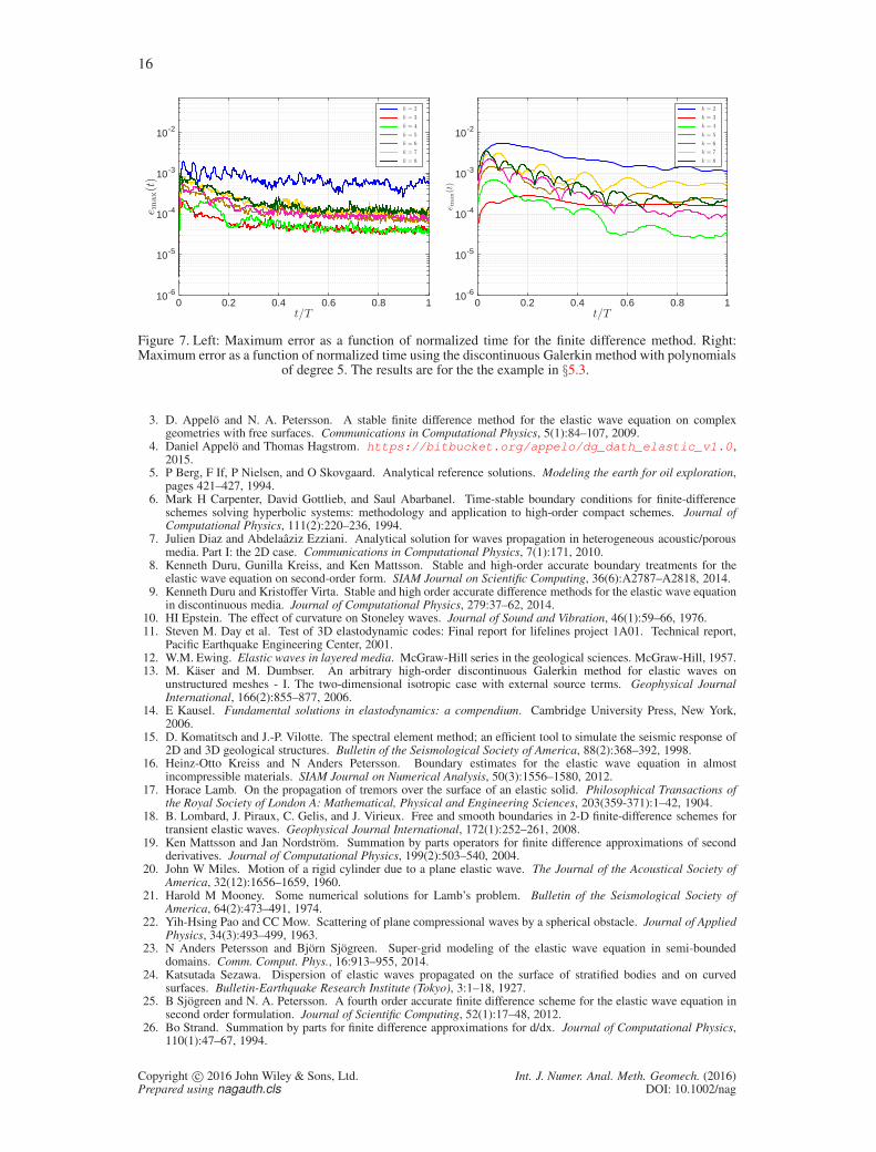
Figure 7 displays the maximum errors as functions of t/T for each k in {2, 3, 4, 5, 6, 7, 8}. It can

be seen that the errors for both methods are of the same magnitude indicating that there is no strong

dependence on k. The errors are slightly better for the finite difference difference method for the

number of periods considered here, however it also appears as if the errors decay faster over time

for the dG method. The better long-time behavior of the dG method is another indication that the

dispersive properties of the dG method are better than that of the finite difference method.

6. SUMMARY

We have presented formulae for particular solutions to the elastic wave equation in cylindrical

geometry. The solutions are freely available as the software PeWe which can be downloaded at

[28].

The solutions were used to compare a finite difference and a discontinuous Galerikin method.

The methods perform about equally well when λ/µ ∼ 1 but the discontinuous Galerkin method out

performs the finite difference method involving surface waves and λ/µ >> 1. The presented results

can serve as a benchmark for future comparison using other numerical methods.

REFERENCES

1. D. Appelo, J. W. Banks, W. D. Henshaw, and D. W. Schwendeman. Numerical methods for solid mechanics onoverlapping grids: Linear elasticity. Journal of Computational Physics, 231(18):6012–6050, 2012.

2. D. Appelo and T. Hagstrom. An energy-based discontinuous Galerkin discretization of the elastic wave equationin second order form. Submitted to CMAME, 2015.


16

0 0.2 0.4 0.6 0.8 110-6

10-5

10-4

10-3

10-2

t/T

e max(t)

k = 2

k = 3

k = 4

k = 5

k = 6

k = 7

k = 8

0 0.2 0.4 0.6 0.8 110-6

10-5

10-4

10-3

10-2

t/T

k = 2

k = 3

k = 4

k = 5

k = 6

k = 7

k = 8

e max(t)

Figure 7. Left: Maximum error as a function of normalized time for the finite difference method. Right:Maximum error as a function of normalized time using the discontinuous Galerkin method with polynomials

of degree 5. The results are for the the example in §5.3.

3. D. Appelo and N. A. Petersson. A stable finite difference method for the elastic wave equation on complexgeometries with free surfaces. Communications in Computational Physics, 5(1):84–107, 2009.

4. Daniel Appelo and Thomas Hagstrom. https://bitbucket.org/appelo/dg_dath_elastic_v1.0 ,2015.

5. P Berg, F If, P Nielsen, and O Skovgaard. Analytical reference solutions. Modeling the earth for oil exploration,pages 421–427, 1994.

6. Mark H Carpenter, David Gottlieb, and Saul Abarbanel. Time-stable boundary conditions for finite-differenceschemes solving hyperbolic systems: methodology and application to high-order compact schemes. Journal ofComputational Physics, 111(2):220–236, 1994.

7. Julien Diaz and Abdelaaziz Ezziani. Analytical solution for waves propagation in heterogeneous acoustic/porousmedia. Part I: the 2D case. Communications in Computational Physics, 7(1):171, 2010.

8. Kenneth Duru, Gunilla Kreiss, and Ken Mattsson. Stable and high-order accurate boundary treatments for theelastic wave equation on second-order form. SIAM Journal on Scientific Computing, 36(6):A2787–A2818, 2014.

9. Kenneth Duru and Kristoffer Virta. Stable and high order accurate difference methods for the elastic wave equationin discontinuous media. Journal of Computational Physics, 279:37–62, 2014.

10. HI Epstein. The effect of curvature on Stoneley waves. Journal of Sound and Vibration, 46(1):59–66, 1976.11. Steven M. Day et al. Test of 3D elastodynamic codes: Final report for lifelines project 1A01. Technical report,

Pacific Earthquake Engineering Center, 2001.12. W.M. Ewing. Elastic waves in layered media. McGraw-Hill series in the geological sciences. McGraw-Hill, 1957.13. M. Kaser and M. Dumbser. An arbitrary high-order discontinuous Galerkin method for elastic waves on

unstructured meshes - I. The two-dimensional isotropic case with external source terms. Geophysical JournalInternational, 166(2):855–877, 2006.

14. E Kausel. Fundamental solutions in elastodynamics: a compendium. Cambridge University Press, New York,2006.

15. D. Komatitsch and J.-P. Vilotte. The spectral element method; an efficient tool to simulate the seismic response of2D and 3D geological structures. Bulletin of the Seismological Society of America, 88(2):368–392, 1998.

16. Heinz-Otto Kreiss and N Anders Petersson. Boundary estimates for the elastic wave equation in almostincompressible materials. SIAM Journal on Numerical Analysis, 50(3):1556–1580, 2012.

17. Horace Lamb. On the propagation of tremors over the surface of an elastic solid. Philosophical Transactions ofthe Royal Society of London A: Mathematical, Physical and Engineering Sciences, 203(359-371):1–42, 1904.

18. B. Lombard, J. Piraux, C. Gelis, and J. Virieux. Free and smooth boundaries in 2-D finite-difference schemes fortransient elastic waves. Geophysical Journal International, 172(1):252–261, 2008.

19. Ken Mattsson and Jan Nordstrom. Summation by parts operators for finite difference approximations of secondderivatives. Journal of Computational Physics, 199(2):503–540, 2004.

20. John W Miles. Motion of a rigid cylinder due to a plane elastic wave. The Journal of the Acoustical Society ofAmerica, 32(12):1656–1659, 1960.

21. Harold M Mooney. Some numerical solutions for Lamb’s problem. Bulletin of the Seismological Society ofAmerica, 64(2):473–491, 1974.

22. Yih-Hsing Pao and CC Mow. Scattering of plane compressional waves by a spherical obstacle. Journal of AppliedPhysics, 34(3):493–499, 1963.

23. N Anders Petersson and Bjorn Sjogreen. Super-grid modeling of the elastic wave equation in semi-boundeddomains. Comm. Comput. Phys., 16:913–955, 2014.

24. Katsutada Sezawa. Dispersion of elastic waves propagated on the surface of stratified bodies and on curvedsurfaces. Bulletin-Earthquake Research Institute (Tokyo), 3:1–18, 1927.

25. B Sjogreen and N. A. Petersson. A fourth order accurate finite difference scheme for the elastic wave equation insecond order formulation. Journal of Scientific Computing, 52(1):17–48, 2012.

26. Bo Strand. Summation by parts for finite difference approximations for d/dx. Journal of Computational Physics,110(1):47–67, 1994.


https://bitbucket.org/appelo/dg_dath_elastic_v1.0

17

27. Magnus Svard and Jan Nordstrom. On the order of accuracy for difference approximations of initial-boundaryvalue problems. Journal of Computational Physics, 218(1):333–352, 2006.

28. Kristoffer Virta and Daniel Appelo. https://bitbucket.org/appelo/pewe , 2015.29. L. C. Wilcox, G. Stadler, C. Burstedde, and O. Ghattas. A high-order discontinuous Galerkin method for wave

propagation through coupled elastic–acoustic media. Journal of Computational Physics, 229(24):9373 – 9396,2010.

A. COEFFICIENTS

The coefficients m(ij) and f in of the linear systems of equations (23)-(24) are computed by

substitution of the solutions (21)-(22) into the boundary or interface conditions (6)-(7). As a result

these entries involves first and second derivatives of the present Bessel and Hankel functions. To

solve the systems using numerical routines for computing values of Bessel and Hankel functions

the coefficients of the linear systems are presented using the following recursion formula

d

drJn(γr) =

γ

2(Jn−1(γr) − Jn+1(γr)) ,

d

drH(2)

n (γr) =γ

2

(

H(2)n−1(γr) −H

(2)n+1(γr)

)

.

(44)

The coefficients of the equations (23) may be written

m11 = (λ+ 2µ)γ2p4

(

H(2)n−2(γpa)− 2H(2)

n (γpa) +H(2)n+2(γpa)

)

+λ

a

(

γp2

(

H(2)n−1(γpa)−H

(2)n+1(γpa)

)

− n2

aH(2)

n (γpa)

)

,

m12 = 2µn

a

(

γs2

(

(H(2)n−1(γsa)−H

(2)n+1(γsa)

)

− 1

aH(2)

n (γsa)

)

,

m21 = 2µn

a

(

1

aH(2)

n (γpa)−γp2

(

H(2)n−1(γpa)−H

(2)n+1(γpa)

)

)

,

m22 = −n2 µ

a2H(2)

n (γsa)− µγ2s4(H

(2)n−2(γsa)− 2H(2)

n (γsa) +H(2)n+2(γsa))

+µ

a

γs2(H

(2)n−1(γsa)−H

(2)n+1(γsa)),

f1 = (λ+ 2µ)γ2p4

(Jn−2(γpa)− 2Jn(γpa) + Jn+2(γpa))

+λ

a

(

γp2

(Jn−1(γpa)− Jn+1(γpa)) +−n2

aJn(γpa)

)

,

f2 = 2µn

a

(

1

aJn(γpa)−

γp2

(Jn−1(γpa)− Jn+1(γpa))

)

.

(45)


https://bitbucket.org/appelo/pewe

18

The coefficients of the equations (24) may be written

m(11)n =

γp2

(

H(2)n−1(γpa)−H

(2)n+1(γpa)

)

,

m(12)n =

n

aH(2)

n (γsa),

m(13)n = −

γ′p2

(

Jn−1(γ′pa)− Jn+1(γ

′pa))

,

m(14)n = −n

aJn(γsa),

m(21)n = −n

aH(2)

n (γpa),

m(22)n = −γs

2

(

H(2)n−1(γsa)−H

(2)n+1(γsa)

)

,

m(23)n =

n

aJn(γ

′pa),

m(24)n = −γs

2(Jn−1(γsa)− Jn+1(γsa)) ,

m(31)n = (λ+ 2µ)

γ2p4

(

H(2)n−2(γpa)− 2H(2)

n (γpa) +H(2)n+2(γpa)

)

+λ

a

(

γp2

(

H(2)n−1(γpa)−H

(2)n+1(γpa)

)

− n2

aH(2)

n (γpa)

)

,

m(32)n = 2µ

n

a

(

γs2

(

H(2)n−1(γsa)−H

(2)n+1(γsa)

)

− 1

aH(2)

n (γsa)

)

,

m(33)n = −(λ′ + 2µ′)

γ′2p4

(

Jn−2(γ′pa)− 2Jn(γ

′pa) + Jn+2(γ

′pa))

− λ′(

1

a

γ′p2

(


′pa))

− n2

a2Jn(γ

′pa)

)

,

m(34)n = −2µ′n

a

(

γ′s2

(Jn−1(γ′sa)− Jn+1(γ

′sa))−

1

aJn(γ

′sa)

)

,

m(41)n = 2µ

n

a

(

(1

aH(2)

n (γpa)−γp2

(

H(2)n−1(γpa)−H

(2)n+1(γpa)

)

)

,

m(42)n = −µ

(

n2

aH(2)

n (γsa) +γ2s4

(

H(2)n−2(γsa)− 2H(2)

n (γsa) +H(2)n+2(γsa)

)

)

+µ

a

γs2

(

H(2)n−1(γsa)−H

(2)n+1(γsa)

)

,

m(43)n = −2µ′n

a

(

(1

aJn(γ

′pa)−

γ′p2

(


′pa))

)

,

m(44)n = µ′

(

n2

aJn(γ

′sa) +

γ′2s4

(Jn−2(γ′sa)− 2Jn(γ

′sa) + Jn+1(γ

′sa))

)

,

− µ′

a

γ′s2

(Jn−1(γ′sa)− Jn+1(γ

′sa))

f (1)n =

γp2

(Jn−1(γpa)− Jn+1(γpa)) ,

f (2)n = −n

aJn(γpa),

f (3)n = (λ+ 2µ)

γ2p4

(Jn−2(γpa)− 2Jn(γpa) + Jn(γpa))

+ λ

(

1

a(Jn−1(γpa)− Jn+1(γpa))−

n2

a2Jn(γpa)

)

,

f (4)n = 2µ

n

a

(

1

aJn(γpa)−

γp2

(Jn−1(γpa)− Jn+1(γpa))

)

.

(46)


19

B. TABULATED CONSTANTS

µ c B

1 ∗ 1.118807339314738 i0.259859421131935

1 1.766356057610045 i0.551757806713995

1 2.185554978245760 −i1.111726166772277

1 2.670175822539088 i0.958432243767886

1 2.955157420561863 −i0.732513991983086

0.1 ∗ 0.362343233711522 i0.008979356435568

0.1 0.579278221572536 i0.061797475082992

0.1 0.728953134331886 −i0.195334916685379

0.1 0.895978188422108 i0.716217080313942

0.1 1.067385352879540 −i1.855812650827352

0.01 ∗ 0.115042076979121 i1.800969171774775 × 10−5

0.01 0.184047312259251 i1.608778558352172 × 10−4

0.01 0.232136819580657 −i5.996559491070863 × 10−4

0.01 0.284650355722595 i0.002791241585515

0.01 0.338604827125379 −i0.010369491587158

0.001 ∗ 0.036395018364438 i1.946610327968597 × 10−8

0.001 0.058228929768223 i1.791032555369920 × 10−7

0.001 0.073461004595573 −i6.806632052120861 × 10−7

0.001 0.090056708451170 i3.250907109941674 × 10−6

0.001 0.107108691805566 −i1.252501580039413 × 10−5

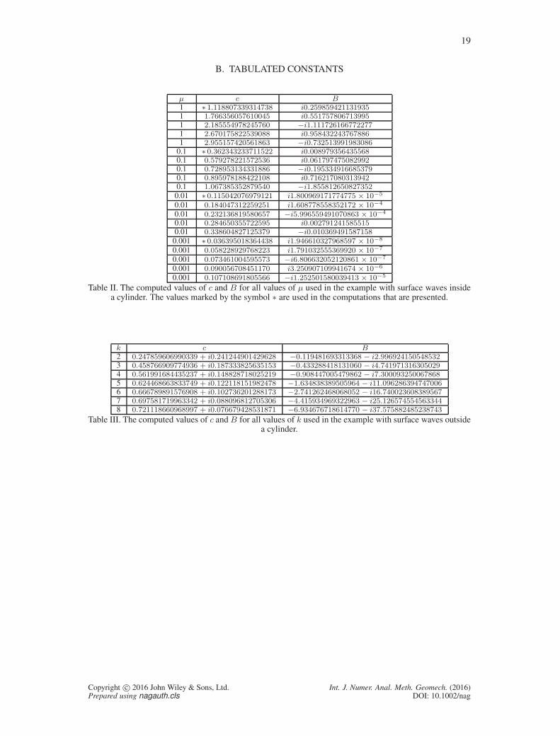
Table II. The computed values of c and B for all values of µ used in the example with surface waves insidea cylinder. The values marked by the symbol ∗ are used in the computations that are presented.

k c B

2 0.247859606990339 + i0.241244901429628 −0.119481693313368 − i2.996924150548532

3 0.458766909774936 + i0.187333825635153 −0.433288418131060 − i4.741971316305029

4 0.561991684435237 + i0.148828718025219 −0.908447005479862 − i7.300093250067868

5 0.624468663833749 + i0.122118151982478 −1.634838389505964 − i11.096286394747006

6 0.666789891576908 + i0.102736201288173 −2.741262468068052 − i16.740023608389567

7 0.697581719963342 + i0.088096812705306 −4.415934969322963 − i25.126574554563344

8 0.721118660968997 + i0.076679428531871 −6.934676718614770 − i37.575882485238743

Table III. The computed values of c and B for all values of k used in the example with surface waves outsidea cylinder.


Formulae and Software for Particular Solutions to the ...appelo/preprints/part_sol_manuscript.pdfat...

Documents

Transcript of Formulae and Software for Particular Solutions to the ...appelo/preprints/part_sol_manuscript.pdfat...