Formula Handbook
80
7th Edition 2012 136 Name__________________________ Course__________________________ Link to Contents Introduction Formula Handbook including Engineering Formulae, Mathematics, Statistics and Computer Algebra http://is.gd/formulahandbook - pdf http://ubuntuone.com/p/dAn - print
-
Upload
brauliodantas -
Category
Documents
-
view
131 -
download
5
description
Formula Handbook
Transcript of Formula Handbook

7th Edition 2012 136
Name__________________________
Course__________________________
Link to Contents
Introduction
FormulaHandbook
includingEngineeringFormulae,Mathematics,Statisticsand Computer Algebra
http://is.gd/formulahandbook - pdf
http://ubuntuone.com/p/dAn - print

Introduction
This handbook was designed to provide engineering students at Aberdeen College with the formulae required for their courses up to Higher National level (2nd year university equivalent).
In order to use the interactive graphs you will need to have access to Geogebra (see 25 ). If you are using a MS Windows operating system and you already have Java Runtime Environment loaded then no changes will be required to the registry. This should mean that no security issues should be encountered. If you have problems see http://www.geogebra.org/cms/en/portable
I have the handbook copied as an A5 booklet with a spiral binding. The covers are printed on thin card rather than paper. It is typed in LibreOffice Writer. Future developments will include more hyperlinks within the handbook and to other maths sites, with all the illustrations in it produced with Geogebra (see 25) or LibreOffice.
Any contributions will be gratefully accepted and acknowledged in the handbook.If you prefer, you can make changes or add to the handbook within the terms of the Creative Commons licence . I will send you a copy the original LibreOffice file on request. Please send me a copy of your work and be prepared to have it incorporated or adapted for inclusion in my version.My overriding concern is for the handbook to live on and be continuously improved.I hope that you find the handbook useful and that you will enjoy using it and that that you will feel inspired to contribute material and suggest hyperlinks that could be added.
Many thanks to my colleagues at Aberdeen College and elsewhere for their contributions and help in editing the handbook. Special thanks are due to Mark Perkins at Bedford College who adopted the handbook for his students, helped to format the contents and contributed to the contents. Without Mark's encouragement this project would have never taken off.
If you find any errors or have suggestions for changes please contact the editor: Peter K Nicol. ([email protected]) ([email protected]) Contents
Peter K Nicol Aberdeenshire,Scotland
7th Edition VI/MMXII
13/03/13136

Contents 1 Recommended Books..................................3
1.1 Maths.................................................3
1.2 Mechanical and Electrical Engineering . .3
2 Useful Web Sites.........................................4
3 Evaluation..................................................6
3.1.1 Accuracy and Precision........................6
3.1.2 Units........................................................6
3.1.3 Rounding................................................6
4 Areas and Volumes......................................7
5 Electrical Formulae and Constants ...............8
5.1 Basic .................................................8
5.2 Electrostatics.......................................8
5.3 Electromagnetism ...............................8
5.4 AC Circuits .........................................9
6 Mechanical Engineering.............................10
6.1.1 Dynamics: Terms and Equations......10
6.1.2 Conversions.........................................10
6.2 Equations of Motion...........................10
6.3 Newton's Second Law........................11
6.3.1 Centrifugal Force.................................11
6.4 Work done and Power........................11
6.5 Energy..............................................11
6.6 Momentum / Angular Impulse..............12
6.7 Specific force / torque values...............12
6.8 Stress and Strain...............................12
6.9 Fluid Mechanics.................................13
6.10 Heat Transfer..................................13
6.11 Thermodynamics..............................14
7 Maths for Computing..................................15
7.1.1 Notation for Set Theory and Boolean Laws ...............................................................15
8 Combinational Logic..................................16
8.1.1 Basic Flowchart Shapes and Symbols.........................................................................16
9 Mathematical Notation – what the symbols mean...........................................................17
9.1.1 Notation for Indices and Logarithms 18
9.1.2 Notation for Functions........................18
10 Laws of Mathematics...............................19
10.1 Algebra...........................................20
10.1.1 Sequence of operations...................20
10.1.2 Changing the subject of a Formula (Transposition)...............................................21
11 The Straight Line ...................................22
12 Quadratic Equations ..............................23
13 Simultaneous Equations with 2 variables....24
14 Matrices.................................................25
15 The Circle...............................................28
15.1.1 Radian Measure................................28
16 Trigonometry...........................................29
16.1.1 Notation for Trigonometry................29
16.2 Pythagoras’ Theorem.......................29
16.3 The Triangle....................................30
16.3.1 Sine and Cosine Rules and Area Formula...........................................................30
16.4 Trigonometric Graphs.......................31
16.4.1 Degrees - Radians Conversion.......33
16.4.2 Sinusoidal Wave................................34
16.5 Trigonometric Identities.....................35
16.6 Multiple / double angles....................35
16.7 Products to Sums.............................36
17 Complex Numbers...................................37
18 Vectors...................................................38
18.1 Co-ordinate Conversion using Scientific Calculators...............................................39
18.2 Graphical Vector Addition..................41
19 Functions................................................42
19.1 Indices and Logarithms.....................42
19.2 Infinite Series and Hyberbolic Functions...............................................................43
Contents p1 9 Notation 1 24 Computer Input

19.3 Exponential and Logarithmic Graphs. .44
19.4 Graphs of Common Functions...........45
20 Calculus ................................................46
20.1.1 Notation for Calculus........................46
20.2 Differential Calculus - Derivatives.......47
20.2.1 Maxima and Minima..........................49
20.2.2 Differentiation Rules.........................49
20.2.3 Formula for the Newton-Raphson Iterative Process............................................50
20.2.4 Partial Differentiation .......................50
20.2.5 Implicit Differentiation.......................50
20.2.6 Parametric Differentiation................50
20.3 Integral Calculus - Integrals...............51
20.3.1 Integration by Substitution...............52
20.3.2 Integration by Parts...........................52
20.3.3 Indefinite Integration.........................53
20.3.4 Area under a Curve..........................53
20.3.5 Mean Value........................................53
20.3.6 Root Mean Square (RMS)...............53
20.3.7 Volume of Revolution ......................54
20.3.8 Centroid..............................................54
20.3.9 Partial Fractions................................54
20.3.10 Approximation of Definite Integrals.........................................................................55
20.3.10.1 Simpson's Rule.......................55
20.3.10.2 Trapezium Method.................55
20.4 Laplace Transforms .........................56
20.5 Approximate numerical solution of differential equations.................................57
20.6 Fourier Series. ...............................58
20.6.1 Fourier Series - wxMaxima method..........................................................................59
21 Statistics.................................................60
21.1.1 Notation for Statistics........................60
21.2 Statistical Formulae..........................61
21.2.1 Regression Line ...............................62
21.2.2 T Test .................................................62
21.2.3 Statistical Tables ..............................63
21.2.3.1 Normal Distribution...................63
21.2.3.2 Far Right Tail Probabilities .....63
21.2.3.3 Critical Values of the t Distribution................................................64
21.2.4 Normal Distribution Curve................65
21.2.5 Binomial Theorem.............................65
21.2.6 Permutations and Combinations.. . .65
22 Financial Mathematics.............................66
23 Recommended Computer Programs..........67
24 Computer Input ......................................68
24.1 wxMaxima Input...............................69
24.1.1 Differential Equations.......................69
24.1.2 Runge-Kutta.......................................69
24.2 Mathcad Input .................................70
24.3 SMath.............................................70
24.4 Spreadsheet procedures ..................71
24.4.1 Find the ‘best fit’ formula for a set of data..................................................................71
24.4.2 Euler's Method...................................71
25 Calibration Error......................................74
26 Mechanical Tables...................................75
26.1.1 Properties of Materials.....................75
26.1.2 Young's Modulus- approximate.......75
27 Periodic Table of The Elements.................76
SI Units - Commonly used prefixes..................77
28 Electrical Tables......................................77
29 THE GREEK ALPHABET.........................78
Contents p1 9 Notation 2 24 Computer Input

1 Recommended Books referred to by author name in this handbook 1.1 Maths
General pre-NC and NC : Countdown to Mathematics; Graham and SargentVol. 1 ISBN 0-201-13730-5, Vol. 2 ISBN 0-201-13731-3
NC Foundation Maths, Croft and DavisonISBN 0-131-97921-3
NC and HN and Degree: Engineering Mathematics through Applications; K Singh Kuldeep Singh, ISBN 0-333-92224-7. (1st Edition) (1)
978-0-230-27479-2 (2nd Edition) (2)www.palgrave.com/science/engineering/singh
Engineering Mathematics, 6th Edition, J BirdISBN 1-8561-7767-X
HN and degree: Higher Engineering Mathematics, 4th Edition, J Bird, J Bird ISBN 0-7506-6266-2
Degree Engineering Mathematics 6th Edition , K A StroudISBN 978-1- 4039-4246-3
-----------------------------------------------------------------------------------------------
1.2 Mechanical and Electrical Engineering
NC Advanced Physics for You, K Johnson, S Hewett et al. ISBN 0 7487 5296 X
Mechanical Engineering
NC and HN Mechanical Engineering Principles, C Ross, J BirdISBN 0750652284
Electrical Engineering
NC and HN Basic Electrical Engineering ScienceIan McKenzie Smith, ISBN 0-582-42429-1
Contents p1 9 Notation 3 24 Computer Input

2 Useful Web Sites
If you use any of the sites below please read the instructions first. When entering mathematical expressions the syntax MUST be correct. See section 24 of this book.Most sites have examples as well as instructions. It is well worth trying the examplesfirst.If you find anything really useful in the sites below or any other site please tell us so that we can pass on the information to other students.
Efunda A US service providing a wealth of engineeringinformation on materials, processes, Maths,unit conversion and more. Excellent calculators (likequickmath). http://www.efunda.com
Mathcentre Try the Video Tutorials. http://www.mathcentre.ac.uk
MC The other stuff is excellent too. Also see http://www.mathtutor.ac.uk
WolframAlpha Almost any maths problem solved!http://www.wolframalpha.com/
BetterExplained It is true – maths and some other topics explained BE better. http://BetterExplained.com/
how to learn maths how to learn maths
Khan Academy The "free classroom of the World"Many video lectures using a blackboardhttp://www.khanacademy.org
Freestudy Mechanical engineering notes and exercises andMaths notes and exercises. http://www.freestudy.co.uk
matek.hu An online calculator which also does calculus and produces graphs. (Based on Maxima). http://www.matek.hu
QuickMath Links you to a computer running MATHEMATICA - the most powerful mathematical software.
http://www.quickmath.com
Mathway Try the problem solver for algebra, trig and calculusand it draws graphs too. See 26 for input syntax.http://www.mathway.com
Just the Maths A complete text book – all in pdf formathttp://nestor.coventry.ac.uk/jtm/contents.htm
Contents p1 9 Notation 4 24 Computer Input

The Open University There are a lot of excellent courses to study and if you want to improve your maths I suggest that you start herehttp://mathschoices.open.ac.uk/Read the text very carefully on all the pages and then go to http://mathschoices.open.ac.uk/routes/p6/index.html and try thequizzes.
OU Learning Space Many courses for many levels - try themhttp://openlearn.open.ac.uk/course/category.php?id=8&perpage=15&page=1
The one below is really useful
Using a Scientific Do you have a Casio fx-83 ES scientific calculator (or a Calculator compatible model) and want to learn how to use it? This
unit will help you to understand how to use the different facilities and functions and discover what a powerful tool this calculator can be! http://openlearn.open.ac.uk/course/view.php?
name=MU123_1
Plus Magazine Plus magazine opens a door to the world of maths, withall its beauty and applications, by providing articles fromthe top mathematicians and science writers on topics asdiverse as art, medicine, cosmology and sport. You canread the latest mathematical news on the site every week,browse our blog, listen to our podcasts and keep up-to-date by subscribing to Plus (on email, RSS, Facebook, iTunes or Twitter).http://plus.maths.org/content/
Paul's Online Math Notes Recommended by June Cardno, Banff and Buchan Collegehttp://tutorial.math.lamar.edu/
Waldomaths Some excellent interactive tools - Equations 1 and 2 in particular for transposition practice.http://www.waldomaths.com/
HND Engineer http://www.hndengineer.co.uk/
Android Scientific Try HEXFLASHOR Calculator
The Narrow Road Maths Explained by Leland McInneshttp://zenandmath.wordpress.com/
If you come across any Engineering or Mathematics sites that might be useful to students on your course please tell me (Peter Nicol) - [email protected]
Contents p1 9 Notation 5 24 Computer Input

3 Evaluation 3.1.1 Accuracy and Precision
Example: Target = 1.234 - 4 possible answers
Not Accurate, not Precise 1.270, 2.130, 0.835, 1.425
Accurate but not Precise 1.231, 1.235, 1.232, 1.236
Precise but not Accurate 1.276, 1.276, 1.276. 1,276
Precise and Accurate 1.234, 1.234, 1.234, 1.234
------------------------------------------------------------------------------------------------------- 3.1.2 Units
MC
Treat units as algebra -
for example KE=12
m v2 where m=5 kg and v=12ms
.
KE=12×5×kg×12×(m
s )2
Standard workshop
KE=12×5×kg×122
×m2
s2 tolerance ±0.2 mm
KE=12×5×122
×kg×m2
s2
KE=360kg⋅m 2
s2 KE=360 J
------------------------------------------------------------------------------------------------------- 3.1.3 Rounding
Do not round calculations until the last line.Round to significant figures preferably in engineering form
Example: A= d 2
4 where d=40
A=1256.637061 A=1.256637061×10³
A=1.257×10³ rounded to 4 sig fig ( A=1257 )There should be at least 2 more significant figures in the calculation than in the answer.
Contents p1 9 Notation 6 24 Computer Input

Volume of a Prism
Area
length
4 Areas and Volumes
Rectangle A=l b
Triangle A= 12
b h
Circle A=πd 2
4A=π r2
C=π d C=2π r
Cylinder V = Area of circular base times height
V cyl=π d 2
4×h V cyl=π r 2×h
Total surface area = A=πd h+ 2π d 2
4
side + 2 ends A=2π r h+ 2π r2
Cone V cone=V cyl
3or V=
πd 2 h12
V=π r 2 h
3
Curved surface area A=π d l2
A=π r l
Total surface area A=π r l+π r2
Sphere V sphere=2V cyl
3V=
πd 3
6V=
4π r3
3
Total surface area A=πd 2 A=4π r2
Contents p1 9 Notation 7 24 Computer Input
l
b
b
h
d
r
h
d
Volume = Area x length(Uniform cross sectional area)
d
hl
d
d

5 Electrical Formulae and Constants Circuit Construction Kit
5.1 BasicUnit symbol
Series Resistors RT=R1R2R3… .
Parallel Resistors1RT
=1R1
1R2
1R3
… . 8
Potential Difference V=I R V
Power P= I V or P= I 2 R or P=V 2
R W
Energy (work done) W=P t J or kWh
Frequency f = 1T
Hz
- - - - - - - - - - - - - - - - - - - - - - - - - - - - - - - - - - - - - - - - - - - - - - - - - - - - - - - 5.2 Electrostatics
Series Capacitors1
CT
=1
C1
1
C 2
1
C3
… . F
Parallel Capacitors CT=C1C2C3 …. F
Charge Q=I t or Q=C V C
Capacitance C=A d=
A 0 r
d F
Absolute Permittivity 0≈8.854×10⁻¹² F/m- - - - - - - - - - - - - - - - - - - - - - - - - - - - - - - - - - - - - - - - - - - - - - - - - - - - - - - 5.3 Electromagnetism
Magnetomotive Force F= I N At
Magnetisation H= I Nℓ
At/m
Reluctance S= l A
=l
o r A At/Wb
Absolute Permeability 0=4×10⁻⁷ H/m- - - - - - - - - - - - - - - - - - - - - - - - - - - - - - - - - - - - - - - - - - - - - - - - - - - - - - - -
Contents p1 9 Notation 8 24 Computer Input

5.4 AC Circuits Unit Symbol
Force on a conductor F=B I ℓ N
Electromotive Force E=B ℓ v V
Instantaneous emf e=E sin V
Induced emf e=N d dt
e=L didt
V
RMS Voltage V rms=1 2×V peak V rms≈0.707V peak V
Average Voltage V AV=2×V peak V AV≈0.637V peak V
Angular Velocity =2 f rad/s16.4.2
Transformation RatiosV s
V p
=N s
N p
=I p
I s
Potential Difference V=I Z V
Power Factor pf=cos(ϕ)
Capacitive Reactance X C=1
2 f C
Inductive Reactance X L=2 f L
Admittance Y= 1Z
S
True Power P=V I cos(ϕ) W
Reactive Power Q=V I sin (ϕ) VAr
Apparent Power S=V I * =P j Q VA
Note: I * is the complex conjugate of the phasor current. See 17
_________________________________________________________Thanks to Iain Smith, Aberdeen College
Contents p1 9 Notation 9 24 Computer Input

6 Mechanical Engineering[K Singh(1) 2–98 especially 32 – 40 and 69 - 73 (2) 2-99]
6.1.1 Dynamics: Terms and Equations
Linear Angulars= displacement (m) = angular displacement (rad)u= initial velocity (m/s) 1= initial velocity (rad/s)v= final velocity (m/s) 2= final velocity (rad/s)a= acceleration (m/s2) = acceleration (rad/s2)t= time (s) t = time (s)- - - - - - - - - - - - - - - - - - - - - - - - - - - - - - - - - - - - - - - - - - - - - - - - - - - - - - - - 6.1.2 Conversions
Displacement s=r
Velocity v=r v= st
=t
Acceleration a=r
2 radians = 1 revolution = 360o , i.e. 1 rad= 3602
o
≈57.3o see 16.4.1
If N = rotational speed in revolutions per minute (rpm), then =2 N
60 rad/s
- - - - - - - - - - - - - - - - - - - - - - - - - - - - - - - - - - - - - - - - - - - - - - - - - - - - - - - - 6.2 Equations of Motion
Linear AngularMC
v=ua t 2=1 t
s=12uv t =
1212t
s=ut12
a t 2 =1 t12 t 2
v 2=u 22 a s 22=1
22
a=v – ut
=2−1
t- - - - - - - - - - - - - - - - - - - - - - - - - - - - - - - - - - - - - - - - - - - - - - - - - - - - - - - - - - - - -
Contents p1 9 Notation 10 24 Computer Input

6.3 Newton's Second Law
Linear Angular
∑ F=ma ∑T= I
where T=F r , I=m k 2 and k = radius of gyration
- - - - - - - - - - - - - - - - - - - - - - - - - - - - - - - - - - - - - - - - - - - - - - - - - - - - - - - - - 6.3.1 Centrifugal Force
CF=m v 2
r
CF=m2 r - - - - - - - - - - - - - - - - - - - - - - - - - - - - - - - - - - - - - - - - - - - - - - - - - - - - - - - - 6.4 Work done and Power
Linear Angular
Work Done WD=F s WD=T
Power
P=Work doneTime taken
=F st
=F v
P=T
- - - - - - - - - - - - - - - - - - - - - - - - - - - - - - - - - - - - - - - - - - - - - - - - - - - - - - - - 6.5 Energy
Linear Angular
Kinetic Energy KE= 12
m v2 KE= 12
I 2
KE= 12
m k 22
Potential Energy PE=m g h
KE of a rolling wheel = KE (linear) + KE (angular)- - - - - - - - - - - - - - - - - - - - - - - - - - - - - - - - - - - - - - - - - - - - - - - - - - - - - - - -
Contents p1 9 Notation 11 24 Computer Input

6.6 Momentum / Angular Impulse
Impulse = Change in momentum MC
Linear AngularFt=m2 v – m1u Tt= I 22− I 11
If the mass does not change: Ft=m v−mu- - - - - - - - - - - - - - - - - - - - - - - - - - - - - - - - - - - - - - - - - - - - - - - - - - - - - - - - 6.7 Specific force / torque values
Force to move a load: F=m g cosm g sin m a
Force to hoist a load vertically =90o F=m gm a=mga
Force to move a load along a horizontal surface =0o F=m gm a
Winch drum torque T app=T FF r I - - - - - - - - - - - - - - - - - - - - - - - - - - - - - - - - - - - - - - - - - - - - - - - - - - - - - - - - 6.8 Stress and Strain
Stress = load / area =FA
Strain = change in length / original length = ll
or =xl
E= Stress / Strain E=
Bending of BeamsMI=y=
ER
2nd Moment of Area (rectangle) I=b d3
12
Including the Parallel axis Theorem I=b d3
12+A h2
Torsion EquationTJ=r=
GL
2nd Moment of Area (cylinder) J=D 4
32− d 4
32- - - - - - - - - - - - - - - - - - - - - - - - - - - - - - - - - - - - - - - - - - - - - - - - - - - - - - - -Thanks to Frank McClean Scott Smith and William Livie, Aberdeen College
Contents p1 9 Notation 12 24 Computer Input

6.9 Fluid Mechanics
Mass continuity m= A V , or m= A C
Bernoulli’s Equationp g
C2
2 g z = constant
orp1
g
C12
2 g z1=
p2
g
C 22
2 g z2zF
Volumetric flow rate Q=A v
Actual flow for a venturi-meter Qactual=A1 cd 2 g h m
f– 1
A1
A2 – 1
Efunda Calculator
Actual flow for an orifice plate Q=A0 cd 2 g h m
f– 1
1 – D0
D1
4
Reynold's Number video
Reynold’s number Re= ρV Dv
Re=V D
Efunda calculator
Darcy formula for head loss h=4 f l v 2
2 g d, h=
4 f l v 2
2 d energy loss
Efunda Calculator
----------------------------------------------------------------------------------------------------- 6.10 Heat Transfer
Through a slab Q=k AT 1 – T 2
x
Through a composite Q= T R
where R=x1
k 1
x2
k 2
1h1
1h2
…
Through a cylindrical pipe Q= T R
where R=
12 R1 h1
ln R2
R1
2 k1
ln R3
R2
2 k 2
1
2 R3 h3
------------------------------------------------------------------------------------------------------
Contents p1 9 Notation 13 24 Computer Input

6.11 Thermodynamics
Boyle’s Law p1V 1= p2 V 2
Charles’s LawV 1
T 1
=V 2
T 2
Combined Gas Lawp1 V 1
T 1
=p2 V 2
T 2
Perfect Gas pV=m R T
Mass flow rate m= A C
Polytropic Process pV n = constant
Isentropic Process
(reversible adiabatic) pV γ = constant where γ=
cP
cV
Gas constant R=c p−cv
Enthalpy (specific) h=u p v
Steady flow energy equation Q=m h2 – h1C2
2
2–
C12
2g z 2 – z1W
Vapours v x=x v g
u x=u fx ug−u f
h x=h fx hg – h f or h x=h fx h f g
___________________________________________________________________Thanks to Richard Kaczkowski, Calgary, Canada and Scott Smith, Aberdeen College.
Contents p1 9 Notation 14 24 Computer Input

7 Maths for Computing
a n a to the base n
a10 decimal; denary ( a d) a 2 binary ( a b)
a16 hexadecimal ( a h) a8 octal ( a o)
-----------------------------------------------------------------------------------------------
103 (1000) kilo 210 1024 kilobyte
106 Mega 220 10242 megabytebut
109 Giga 230 10243 gigabyte
1012 Tera 240 10244 terabyte
1015 Peta 250 10245 petabyte_____________________________________________________________ 7.1.1 Notation for Set Theory and Boolean Laws
[J Bird pp 377 - 396]
E universal set
A={a , b , c …} a set A with elements a ,b , c etc
a∈A a is a member of A B⊂A
{ } the empty set ( Ø is also used)
B⊂A B is a subset of A
A∪B ABSet theory Boolean
∪ union ∨ OR
∩ intersection ∧ ⋅ AND A∩B A⋅B
A' complement of A A NOT
A' A
Contents p1 9 Notation 15 24 Computer Input
E
A B
E
A B
EA B
E
B
A
E
E
A B.a
.b .c

8 Combinational Logic
A0=A A⋅0=0
A1=1 A⋅1=A
A⋅A=A AA=A
A A=0 AA=1
A=A
A⋅B=B⋅A AB=BA
A⋅BC =A⋅BA⋅C
AB⋅C =AB⋅AC
A⋅B⋅C =C⋅A⋅B ABC=CAB
A⋅AB =A AA⋅B =A
De Morgan's Laws
A⋅B⋅C⋅...=ABC... ABC...=A⋅B⋅C⋅...
------------------------------------------------------------------------------------------------------ 8.1.1 Basic Flowchart Shapes and Symbols
Start / End Input / Output
Action or Process Connector
Decision Flow Line
______________________________________________________________
Contents p1 9 Notation 16 24 Computer Input

9 Mathematical Notation – what the symbols meanMC
∈ is a member of. ( x∈ℝ means x is a member of ℝ )
ℕ the set of natural numbers 1, 2, 3, ........
ℤ the set of all integers ....., -2, -1, 0, 1, 2, 3, ......
ℚ the set of rational numbers including ℤ and
fractions pq
; p , q∈ℤ
ℝ the set of all real numbers. Numbers represented bydrawing a continuous number line.
ℂ the set of complex numbers. Numbers represented bydrawing vectors.
.˙. therefore
w.r.t. with respect to
∗ used as a multiplication sign (× ) (in computer algebra)
^ used as “power of” ( x y ) in computer algebra
≠ not equal to
≈ approximately equal to
greater than. x2 means x is greater than and not equal to 2
≥ greater than or equal to.
less than. a2 means a is less than and not equal to 2. ≤ less than or equal to.
a≤x≤b x is greater than or equal to a and less than or equal to b
ab abbreviation for a×b or a∗b or a⋅b
a×10n a number in scientific (or standard) form. ( 3×103=3000 )use EXP or ×10x key on a calculator
n ! “ n factorial” n×n – 1×n – 2×n−3×...×1
Contents p1 9 Notation 17 24 Computer Input

A∝B implies A=k B where k is a constant (direct variation)
∣x∣ the modulus of x . The magnitude of the number x ,irrespective of the sign. ∣−3∣=3=∣3∣
∞ infinity
⇒ implies
- - - - - - - - - - - - - - - - - - - - - - - - - - - - - - - - - - - - - - - - - - - - - - - - - - - - - - - - 9.1.1 Notation for Indices and Logarithms
MC
a n abbreviation for a×a×a×a ...×a (n terms). see 19.1
x▄ or ^ or x y or y x or ab on a calculator.
a the positive square root of the number a . x=x12=x0.5
k a k th root of a number a . 3 8=2 k a=a1k .
e x exp x (2.71828.... to the power of x ). See 19.1.
loge( x) ln x on a calculator. The logarithm of x to the base e
log10( x) log x on a calculator. The logarithm of x to the base 10
- - - - - - - - - - - - - - - - - - - - - - - - - - - - - - - - - - - - - - - - - - - - - - - - - - - - - - - - 9.1.2 Notation for Functions
f x a function of x . Also seen as g x , h x , y x
f −1x the inverse of the function labelled f x
g ° f the composite function - first f then g . or g f x .
------------------------------------------------------------------------------------------------------
Contents p1 9 Notation 18 24 Computer Input

10 Laws of Mathematics
Associative laws - for addition and multiplication
abc =ab c a b c=a bc- - - - - - - - - - - - - - - - - - - - - - - - - - - - - - - - - - - - - - - - - - - - - - - - - - - - - - - -
Commutative laws - for addition and multiplication
ab=ba but a – b≠b−a
a b=b a butab≠
ba
- - - - - - - - - - - - - - - - - - - - - - - - - - - - - - - - - - - - - - - - - - - - - - - - - - - - - - - -Distributive laws - for multiplication and division
a bc =a ba cbc
a=
ba
ca
- - - - - - - - - - - - - - - - - - - - - - - - - - - - - - - - - - - - - - - - - - - - - - - - - - - - - - - - Arithmetical Identities
x0=x x×1=x x×0=0- - - - - - - - - - - - - - - - - - - - - - - - - - - - - - - - - - - - - - - - - - - - - - - - - - - - - - - -
Algebraic Identities K Singh pp 73 – 75
ab2=abab=a22 a bb2 a 2 – b2=ab a−b
ab3=aba22 a bb2=a 33 a2 b3 ab2b3 see 19.4
- - - - - - - - - - - - - - - - - - - - - - - - - - - - - - - - - - - - - - - - - - - - - - - - - - - - - - - - Other useful facts
a – b=a−bab=a÷b=a
1×
1b
a−−b=a−−b=ab- - - - - - - - - - - - - - - - - - - - - - - - - - - - - - - - - - - - - - - - -
ab
cd=
a db cb d
ab×
cd=
a cb d
see 20.3.9, 5
ab÷
cd=
ab×
dc
MC
abcd =acadbcbd FOIL- - - - - - - - - - - - - - - - - - - - - - - - - - - - - - - - - - - - - - - - - - - - - - - - - - - - - - - -
MC
Contents p1 9 Notation 19 24 Computer Input

10.1 Algebra 10.1.1 Sequence of operations
[K Singh (1) 40-43 (2) 40-43]
Sequence of operations - the same sequence as used by scientific calculators.
------------------------------------------------------------------Brackets come before
-------------------------------------------------------------------Of x 2, x , sin x , e x , comes before
“square of x , sine of x-------------------------------------------------------------------Multiplication × comes before
Division ÷ comes before
-------------------------------------------------------------------Addition comes before
Subtraction −
-------------------------------------------------------------------
3sin a x2b−5 would be read in this order
left bracket
x squared
times a
plus b
right bracket
sine of the result ( sin a x 2b )
times 3
minus 5
Contents p1 9 Notation 20 24 Computer Input

10.1.2 Changing the subject of a Formula (Transposition)[K Singh (1) 53-66 (2) 53-56]
An equation or formula must always be BALANCED - whatever mathematical operation you do to one side of an equals signmust be done to other side as well. (to all the terms)
You can’t move a term (or number) from one side of the equals sign tothe other. You must UNDO it by using the correct MATHEMATICAL operation.
UNDO with − and − with
UNDO × with ÷ and ÷ with ×
UNDO with x 2 and x 2 with
UNDO x n with n and
n with x n
UNDO sin x with sin−1 x and sin−1 x with sin x
UNDO e x with ln x and ln x with e x
UNDO 10 x with log10 x and log10 x with 10 x
UNDOdydx
with ∫dx and ∫dx withdydx
UNDO L [ y ] with L−1[ y ] and L−1
[ y ] with L [ y ]
etc
Generally (but not always) start with the terms FURTHEST AWAY from the new subject FIRST.
Think of the terms in the formula as layers of an onion - take the layers off one by one.
a x2b
Try this first http://www.waldomaths.com/Equation3NLW.jspThere is a link to Equations 1 if you need a bit more help.
MC
Contents p1 9 Notation 21 24 Computer Input
+ +=5a - 7 7 3b 7

11 The Straight Line[K Singh (1) 100–108 (2) 101-110]
The general equation of a straight line of gradient m cutting the yaxis at 0,c is
y=m xc
where the gradient
m= y2 – y1
x2−x1or
dydx= y2 – y 1
x 2−x1. See 20.1.1, 20.2 and 16.3
or y1=m x1+ c (1)y 2=m x 2+ c (2) then (1) – (2) and solve for m (then c )
Also:
A straight line, gradient m passing through a ,b has the equation:
y−b=mx−a
Also see 24.3.1 , back to 20.2.3, 20.5, 21.2.1, 20.3.10, 13, MC
------------------------------------------------------------------------------------------------------
Contents p1 9 Notation 22 24 Computer Input
x1
x2
y2
y1
c
( x2 , y
2 )
( x1 , y
1 )
y
xdx
dy+ve gradient
-ve gradient

12 Quadratic Equations[K Singh (1,2) 86 - 90 & (1) 109 - 113 (2) 110-113]
Focus
F=(−b2a
,−(b2
−4 a c−1)4 a )
Geogebra quadraticMC
The real solutions (roots) x1 and x 2 of the equation a x2b xc=0 are the value(s) of x where y=a x2b xc crosses the x axis.
The solutions (roots) x1 and x 2 of a x2b xc=0 are given by the Quadratic Formula.
x=−b(2 a)
±√ (b2 – 4 a c)
(2 a)or x=
−b± b2 – 4 a c 2 a
Definition of a root: The value(s) of x which make y equal to zero.….........................................................................................................................Also:
a x2b xc=0
x2
ba
xca=0
x b
a 2
2
d 2=0
where d 2=
ca−
ba 2
2
see 22.4
If y=k xA2B the turning point is −A , B Geogebra
back to 13, -------------------------------------------------------------------------------------------------------
Contents p1 9 Notation 23 24 Computer Input
y=a x 2b xc-ve a
+ve a
x=−b2 a
a minimum turning point
y
x
c
x1 x
2
F

13 Simultaneous Equations with 2 variables[K Singh (1) pp 90-98 (2) 90-99]
General method:
Write down both equations and label (1) and (2).a x+b y=e (1)c x+d y= f (2)Multiply every term on both sides of (1) by c and every term onboth sides of (2) by a and re-label as (3) and (4).c a x+c b y=c e (3)a c x+a d y=a f (4)Multiply every term on both sides of (4) by -1 and re-label.
c a x+c b y=c e (3)−a c x−a d y=−a f (5)Add (3) to (5) to eliminate xCalculate the value of y
Substitute the value of y into equation (1)Calculate the value of x MC
Check by substituting the values of x and y into (2)- - - - - - - - - - - - - - - - - - - - - - - - - - - - - - - - - - - - - - - - - - - - - - - - - - - - Graphical Solution
a x+b y=e
c x+d y= f
If f x =g x then f x – g x =0 - also see 11 and 12
_________________________________________________________
Contents p1 9 Notation 24 24 Computer Input
x
y
x1
x2
y1
y2

14 Matrices[K Singh (1) pp 507 – 566 (2) 560-635]
Notation:
Identity = [1 0 0 ..0 1 0 ..0 0 1 ... . . ..
]A m×n matrix has m rows and n columns.
aij an element in the i th row and j th column.-----------------------------------------------------------------------------------------------------
If A=[a11 a12
a21 a22] and B=[b11 b12
b21 b22 ]
then AB=[ a11b11 a12b12
a21b21 a 22b22]
and A×B=[ a11b11a12b21 a11b12a12b22
a21 b11a22 b21 a21b12a22 b22] ColumnsA=RowsB
-------------------------------------------------------------------------------------------------------Solution of Equations 2 x 2
If A X=B then X=A−1 B [ a bc d ][ x
y]=[ ef ]
If A=[a bc d ]
then the inverse matrix,
A−1=
1det A [ d −b
−c a ] , a d−b c≠0 MC
where the Determinant det A=∣a bc d∣=ad−bc
- - - - - - - - - - - - - - - - - - - - - - - - - - - - - - - - - - - - - - - - - - - - - - - - - - - - - - - -
Contents p1 9 Notation 25 24 Computer Input

Inverse Matrix, 3 x 3 (and larger square matrices)
Start with [a11 a12 a13
a21 a22 a23
a31 a32 a33∣∣
1 0 00 1 00 0 1] carry out row operations to:
[1 0 00 1 00 0 1∣∣
b11 b12 b13
b21 b22 b23
b31 b32 b33] where [
b11 b12 b13
b21 b22 b23
b31 b32 b33]=A−1
Determinant of a 3 x 3 matrix
det A=∣a11 a12 a13
a21 a22 a23
a31 a32 a33∣=a11∣a22 a23
a32 a33∣−a12∣a21 a23
a31 a33∣a13∣a21 a22
a31 a32∣
or use Sarrus' Rule as below
det A=∣a11 a 12 a13
a21 a 22 a23
a31 a 32 a33∣=[
a11 a12 a13
a21 a22 a23
a31 a32 a33]a11 a12
a 21 a 22
a 31 a32
detA=a11a 22a33a12 a23 a31a 13a21 a32
−a31 a22 a13−a32 a23 a11−a33 a21 a12
-----------------------------------------------------------------------------------------------Thanks to Richard Kaczkowski, Calgary, Canada.
Contents p1 9 Notation 26 24 Computer Input
_ _ _
+ + +

Inverse of a 3 by 3 matrices by using co-factors
A=[a b cd e fg h i ] A−1=
1detA
(adjA)
where adjA is the adjoint (adjunct) matrix of AadjA=CT where CT = the transpose of the
co-factors of A
Co-factors
cf (a)=det [ e fh i ] cf (b)=−det[ d f
g i ] cf (c)=det [ d eg h ]
cf (d )=−det [ b ch i ] cf (e)=det [ a c
g i ] cf ( f )=−det[ a bg h]
cf (g)=det [ b ce f ] cf (h)=−det [ a c
d f ] cf (i)=det [ a bd e ]
Be careful of place signs! [+ − +− + −+ − + ]
Co-factor Matrix C=[cf (a) cf (b) cf (c)cf (d ) cf (e ) cf ( f )cf ( g) cf (h) cf (i) ]
Then, transpose the Co-factor Matrix (rows to columns)
Adjoint (Adjunct) Matrix CT=[cf (a) cf (d ) cf (g )cf (b) cf (e) cf (h)cf (c) cf ( f ) cf (i) ] = adjA
_________________________________________________________
Contents p1 9 Notation 27 24 Computer Input

15 The Circle
A Minor Sector C Minor Segment
B Major Sector D Major Segment
- - - - - - - - - - - - - - - - - - - - - - - - - - - - - - - - - - - - - - - - - - - - - - - - - - - - - - - -
The equation x – a 2 y – b2=r 2 represents a circle centre a , b and radius r .
Parametric
x=a+r cos t , y=b+r sin t
------------------------------------------------------------------------------------------------------ 15.1.1 Radian Measure
A radian: The angle θ subtended (ormade by) an arc the samelength as the radius of a circle.Notice that an arc is curved.
BE.com degrees and radiansGeogebra Radians
See also 16.4.1
Contents p1 9 Notation 28 24 Computer Input
A
B
C
D
r
a
b
y
x
(x,y)
r
rr
θ

Rb
a
16 Trigonometry[K Singh (1) 167-176 (2) 171-234]
16.1.1 Notation for Trigonometry
Labelling of a triangle
sin the value of the sine function of the angle
cos the value of the cosine function of the angle
tan the value of the tangent function of the angle
=sin−1 b arcsin b the value of the basic angle whose sine function
value is b . −90o≤o≤90o or −2 ≤≤2
=cos−1 b arccos b the value of the basic angle whose cosine function
value is b . 0o≤o≤180o or 0≤≤
=tan−1 b arctan b the value of the basic angle whose tangent function
value is b . −90o≤o≤90o or −2 ≤≤2
------------------------------------------------------------------------------------------------------ 16.2 Pythagoras’ Theorem
In a right angled triangle, with hypotenuse, length R ,and the other two sides of lengths a and b , then
R2=a2b2
or R= a2b2
use of Pythagoras' Theorem BE surprising uses Pythagorean distance BE pythagorean distanceInteractive proof http://www.sunsite.ubc.ca/LivingMathematics/V001N01/UBCExamples/Pythagoras/pythagoras.html
- - - - - - - - - - - - - - - - - - - - - - - - - - - - - - - - - - - - - - - - - - - - - - - - - - - - - - - - -
Contents p1 9 Notation 29 24 Computer Input
A
B C
b
a
c

A
H O
θ
16.3 The Triangle
In a right angled triangle, with hypotenuse, (which is the longest side), of length H ,
SOHCAHTOA
The other two sides have lengths A (adjacent, or next to angle )and O (opposite to angle ) then
MC
sin (θ)= OH
cos(θ)= AH
tan(θ)=OA
see also 18.1
and 11------------------------------------------------------------------------------------------------------ 16.3.1 Sine and Cosine Rules and Area Formula
[K Singh (1) 187-192 (2) 195-191]
In any triangle ABC, where A is the angle at A, B is the angle at B and Cis the angle at C the following hold:
Sine Rulea
sin (A)=
bsin (B)
=c
sin(C)
orsin (A)
a=
sin (B)b
=sin(C)
chttp://www.ies.co.jp/math/java/trig/seigen/seigen.html
Cosine Rule
cos(A)=(b2+c2 – a2)
(2b c)
or a 2=b2+ c2 – 2b c cos(A)http://www.ies.co.jp/math/java/trig/yogen1/yogen1.html
Area Formula
Area = b c sin(A)
2-------------------------------------------------------------------------------------------------------
Contents p1 9 Notation 30 24 Computer Input
C
A
B
b
a
c

16.4 Trigonometric Graphs and Equations[K Singh (1) 177- 202 (2) 181- 210]
MCRadians i.e. no units - horizontal axis is usually time.
y=sin (t)
y=cos( t )
Contents p1 9 Notation 31 24 Computer Input
t
y
Calculator answer
Calculator answer

Trigonometric Graphs - degrees
y=sin (xo)
Geogebra Sine wave slider http://www.ies.co.jp/math/java/trig/graphSinX/graphSinX.html
y=cos (x o)
Geogebra Cosine wave slider http://www.ies.co.jp/math/java/trig/graphCosX/graphCosX.html
Contents p1 9 Notation 32 24 Computer Input
Calculator answer
Calculator answer

y=tan (xo)
------------------------------------------------------------------------------------------------------ 16.4.1 Degrees - Radians Conversion
[K Singh (1) 192-195 (2) 201-204]
0, 30, 45, 60, 90, 120, 135, 150, 180, 210, 225, 240, 270, 300 315, 330, 360
0 6
4
3
2
23
34
56
76
54
43
32
53
74
116
2
Degrees to radians x o÷180×= rad
Radians to degrees rad÷×180=x o
=1 radian Geogebra Radians
BE degrees and radians see 6.1.2
------------------------------------------------------------------------------------------------------
Contents p1 9 Notation 33 24 Computer Input
Calculator answer
r
rr

+(-)
(-)
+
16.4.2 Sinusoidal Wave[K Singh (1) 195-202 (2) 204-212]
see 20.6, 5.4
-------------------------------------------------------------------------------------------------------Thanks to Mark Perkins, Bedford College
Unit Circle-------------------------------------------------------------------------------------------------------
Odd Function Even Function
Saw Tooth Square Wave
Contents p1 9 Notation 34 24 Computer Input
Period = 2
V=R sin t
= phase angle
[Frequency = 2 ]
= phase shift
R
t
θ sin(θ)
cos(θ)
1
0
+
(-)
θ

16.5 Trigonometric Identities[K Singh (1) 203-213 (2) 212-223]
tan(A)=sin (A)cos(A)
cot (A)=1
tan (A)=
cos (A)sin (A)
, (the cotangent of A )
- - - - - - - - - - - - - - - - - - - - - - - - - - - - - - - - - - - - - - - - - - - - - - - - - - - - - - - -
sec(A)= 1cos(A)
, (secant of A ), cosec(A)= 1sin (A)
, (cosecant of A )
- - - - - - - - - - - - - - - - - - - - - - - - - - - - - - - - - - - - - - - - - - - - - - - - - - - - - - - -
sin2(A)+ cos2(A)=1 entered as (sin (A))2+ ( cos(A))
2
- - - - - - - - - - - - - - - - - - - - - - - - - - - - - - - - - - - - - - - - - - - - - - - - - - - - - - - - sin (−θ)=−sin (θ) (an ODD function)
cos −=cos (an EVEN function)------------------------------------------------------------------------------------------------ 16.6 Multiple / double angles
[K Singh (1) 213-222 (2) 223-234]
sin AB=sin A cos Bcos Asin B sin (2 A)=2 sin A cos A
sin A – B=sin Acos B – cos Asin B
cos AB=cos Acos B – sin Asin B
cos2 A=cos2 A – sin2 A=2 cos2 A−1
cos2 A=12cos 2 A1
cos2 A=1−2sin2 A
sin2 A= 121−cos 2 A
cos A – B=cos Acos Bsin Asin B
tan AB= tan Atan B1 – tan A tan B
tan 2 A= 2 tan A1 – tan2 A
tan A−B= tan A−tan B1tan A tan B
- - - - - - - - - - - - - - - - - - - - - - - - - - - - - - - - - - - - - - - - - - - - - - - - - - - - - - - -
Contents p1 9 Notation 35 24 Computer Input

16.7 Products to Sums
sin A cos B=12sin ABsin A−B
cos Asin B= 12sin AB−sin A−B
cos Acos B= 12cos ABcos A−B
sin Asin B=12cosA−B−cos AB
- - - - - - - - - - - - - - - - - - - - - - - - - - - - - - - - - - - - - - - - - - - - - - - - - - - - - - - - -Sums to Products
sin Asin B=2sin AB2 cos A – B
2
sin A−sin B=2 cos AB2 sin A – B
2
cos Acos B=2cos AB2 cos A – B
2
cos A−cos B=−2 sin AB2 sin A – B
2 -----------------------------------------------------------------------------------------------------
Contents p1 9 Notation 36 24 Computer Input

Re
Im
jb
a
r
θ
Argand Diagram
17 Complex Numbers[K Singh (1) 463-506 (2) 513-559]
Notation for Complex NumbersBE - imaginary numbers
j symbol representing −1 . ( i used on most calculators)(defined as j2
=−1 )
a j b a complex number in Cartesian (or Rectangular) form( xy i on a calculator). a , b∈ℝ , j b imaginary part.
z a complex number z=a j b (or xy i )
r a complex number in polar form
z complex conjugate of the complex numberIf z=a j b then the complex conjugate z=a – j b or if z=r then the complex conjugate z=r −
z=a j b=rcos j sin =r =r e j where j2=−1- - - - - - - - - - - - - - - - - - - - - - - - - - - - - - - - - - - - - - - - - - - - - - - - - - - - - - - - -Modulus, r=∣z∣= a2b2 (or magnitude) see 17.2, 17.2
Argument, =arg z=tan−1 ba
(or angle)BE - Complex arithmetic - better explained
Addition a jbc j d =ac j bd
Multiplication a jbc jd Divisiona jbc− jd c jd c− jd
Polar Multiplication z 1 z2=r1 1×r2 2=r 1 r 212
Polar Division z 1
z 2
=r1 1
r2 2
=r 1
r 2
1−2
See also: 18.1 Co-ordinate conversion MC
- - - - - - - - - - - - - - - - - - - - - - - - - - - - - - - - - - - - - - - - - - - - - - - - - - - - - - - - -De Moivre's Theorem
(rθ)n=rn(nθ)=r n(cos(nθ)+ j sin (nθ)) r = r 2
http://www.justinmullins.com/home.htm
____________________________________________________________
Contents p1 9 Notation 37 24 Computer Input

x
a
b
y
(a,b)
ai
bjr
θ
18 VectorsNotation for Graphs and Vectors [K Singh (1) 567-600 (2) 636-671]
x , y the co-ordinates of a point, where x is the distance from the y axis and y is the distance from the x axis
v a vector. Always underlined in written work
AB a vector
a ib j a vector in Cartesian form (Rectangular form) where i is a horizontal 1 unit vector and j is a vertical 1 unit vector.
r a vector in polar form (where r=∣v∣ ) )
ab a vector in Component form (Rectangular Form)
∣v∣ modulus or magnitude of vector v .
- - - - - - - - - - - - - - - - - - - - - - - - - - - - - - - - - - - - - - - - - - - - - - - - - - - - - - - - -Vectors
A point a ,b A vector v=ab or v=r
MC
Vector Addition ab c
d = acbd Geogebra and 18.2
see also 18.1 Co-ordinate Conversion
Scalar Product a×b=∣a∣∣b∣cos(θ)
Dot Product a⋅b=a1 b1a2b2a3 b3 ...
where a=a1
a 2
a3
. and b=
b1
b2
b3
.
-------------------------------------------------------------------------------------------------------
Contents p1 9 Notation 38 24 Computer Input
x
θ
a
b

18.1 Co-ordinate Conversion using Scientific Calculators
R to P Rectangular to Polar xy to r ( x jy to r )
P to R Polar to Rectangular r to xy ( r to x jy )
see also 16.3
Casio Natural Display and Texet EV-S Edit keystrokes for your calculator
R to P SHIFT Pol( x SHIFT , y ) = rθ
out
P to R SHIFT Rec( r SHIFT , θ ) =xy
out
Casio S-VPAM and new Texet Edit keystrokes for your calculator
R to P SHIFT Pol( x SHIFT , y ) = r out RCL tan out
P to R SHIFT Rec( r SHIFT , ) = x out RCL tan y out
Sharp WriteView
R to P x,
(x , y)y 2ndF r r ,θ out
P to R r,
(x , y)θ 2ndF x y x , y out
Sharp ADVANCED D.A.L. Edit keystrokes for your calculator
R to P x 2ndF , y 2ndF → rθ r out out
or MATH 1 r out 2ndF ⋅ out
P to R r 2ndF , 2ndF → x y x out y out
or MATH 2 x out 2ndF ⋅ y out
Old Casio fx & VPAM
R to P x SHIFT RP y = r out SHIFT X Y out
P to R r SHIFT PR = x out SHIFT X Y y out
Contents p1 9 Notation 39 24 Computer Input

Texet - albert 2
R to P x INV x y y RP r out INV x y out
P to R r INV x y PR x out INV x y y out
Casio Graphics (1)R to P SHIFT Pol( x SHIFT , y ) EXE r out ALPHA J EXE out
P to R SHIFT Rec( r SHIFT , ) EXE x out ALPHA J EXE y out
Casio Graphics (2)
R to P FUNC 4 MATH 4 COORD 1 Pol( x , y ) EXE r ALPHA J EXE
P to R FUNC 4 MATH 4 COORD 1 Rec( r , ) EXE x ALPHA J EXE y
Casio Graphics (7 series)R to P OPTN ▶ F2 ▶ ▶ Pol( x , y ) EXE r , out
R to P OPTN ▶ F2 ▶ ▶ Rec( r , ) EXE x , y out
Old Texet and old Sharp and some £1 calculatorsYou must be in Complex Number mode.
2ndF CPLX
R to P x a y b 2ndF a r out b out
P to R r a b 2ndF b x out b y out
Texas - 36X
R to P x x↔ y y 3rd RP r out x↔ y out
P to R r x↔ y 2nd P R x out x↔ y y out
Contents p1 9 Notation 40 24 Computer Input

Texas Graphics (TI 83)
R to P 2nd Angle R Pr ( x , y ) ENTER r out
2nd Angle R P ( x , y ) ENTER out
P to R 2nd Angle P R x ( r , ) ENTER x out
2nd Angle P R y ( r , ) ENTER y out
Sharp Graphics
R to P MATH (D)CONV (3) xy r ( x , y ) ENTER r out
MATH (D)CONV (4) xy ( x , y ) ENTER out
P to R MATH (D)CONV (5) r x ( r , ) ENTER x out
MATH (D)CONV (6) r y ( r , ) ENTER y out
Insert the keystrokes for your calculator here (if different from above)R to P
P to R
------------------------------------------------------------------------------------------------------Degrees to Radians ÷180× Radians to degrees ÷×180_____________________________________________________________
18.2 Graphical Vector Addition
Contents p1 9 Notation 41 24 Computer Input

19 Functions
19.1 Indices and Logarithms[K Singh (1,2) 7-11, (1) 223-245 (2) 235-259]
Rules of Indices: notation 9.1.1MC
1. am×an =amn
2. am
a n =am−n
3. amn =amn
4. a m
n =n am
a 1
n =
n a
5. k a−n =kan
Also,
a 0=1 x=x12=x0.5 and
2 a= a
a1=a n a=b⇔bn
=a
------------------------------------------------------------------------------------------------------Definition of logarithms
If N=a n then n=loga(N )
- - - - - - - - - - - - - - - - - - - - - - - - - - - - - - - - - - - - - - - - - - - - - - - - - - - - - - - - -Rules of logarithms: MC
1. log A×B =log (A)+ log (B)
2. log AB =log (A)– log(B)
3. log (An) =n log (A)
4. loga N =logb Nlogb a
------------------------------------------------------------------------------------------------------exp (x)=e(x) loge( x)=ln( x) log10( x)=lg (x)
------------------------------------------------------------------------------------------------------
Contents p1 9 Notation 42 24 Computer Input

19.2 Infinite Series and Hyberbolic Functions[K Singh (1) pp 246-346, 338-346 (2) 259-270, 358-369]
e x=1x
1!
x2
2!
x3
3 !
x 4
4 !
x5
5!
x6
6!
x7
7 !... for ∣x∣∞
BE exponential functions better explained
sin x=e jx−e− jx
j2 =x− x3
3!
x5
5!−
x7
7 !... for ∣x∣∞
cos x= e jxe− jx
2 =1− x2
2 !
x 4
4 !−
x6
6 !... for ∣x∣∞
ln x=x−1
1–x−12
2x−13
3−... for 0x≤2
BE- demystifying the natural logarithm
- - - - - - - - - - - - - - - - - - - - - - - - - - - - - - - - - - - - - - - - - - - - - - - - - - - - - - - - -Hyperbolic Functions
- definitions [K Singh (1) 246-247 (2) 259-260]
MC pronunciation
sinh x=ex−e−x
2 =x x3
3!
x5
5!
x7
7!... “shine x”
cosh x=e xe−x
2 =1 x2
2!
x4
4!
x6
6!... “cosh x”
tanh x=e x−e−x
e xe−x “thaan x”
______________________________________________________________
k ea x slider k lna x slider
Contents p1 9 Notation 43 24 Computer Input
y = ex y = x
y = ln x
y = cosh x
y = sinh x
y = sinh x
y = tanh x
y = tanh x

19.3 Exponential and Logarithmic Graphs
Contents p1 9 Notation 44 24 Computer Input

19.4 Graphs of Common Functions
y=a x3b x 2c xd y=a x4b x3c x2d x f
y=axb y=x 2 and y= x
y=k 1−e− t y=k e− tb
Contents p1 9 Notation 45 24 Computer Input

20 Calculus
20.1.1 Notation for Calculussee also section 9
Differentiation
dydx
the first derivative of y where y is a function of x (Leibniz)
Also see 11
f ' x the first derivative of f x . (as above). (Euler)
v the first derivative of v w.r.t. time. (Newtonian mechanics)
D u the first derivative of u
d 2 y
dx2 the second derivative of y w.r.t x . The dydx
of dydx
f ' ' x the second derivative of f x . ( f 2x is also used)
v the second derivative of v w.r.t. time. (Newtonian mechanics)
∂ z∂ x
the partial derivative of z w.r.t. x . ( ∂ “partial d”)
x a small change (increment) in x . ( “delta”)
------------------------------------------------------------------------------------------------------Integration
∫ the integral sign (Summa)
∫ f xdx the indefinite integral of f x (the anti-differential of f x )
∫a
b
f xdx the definite integral of f x from x=a to x=b
the area under f x between x=a and x=b
F x the primitive of f x (∫ f xdx without the c )
L [ f t ] the Laplace operator (with parameter s )
-------------------------------------------------------------------------------------------------------BE - gentle introduction to learning Calculus discovring pi - betterexplained.com
Contents p1 9 Notation 46 24 Computer Input

20.2 Differential Calculus - Derivatives
[K Singh (1) pp 258 - 358 (2) 271-398]dydx
y or f x dydx
or f ' x See 11 , 11
________________________________________________ MC
x n n xn−1
sin x cos x
cos x −sin x
e x e x
ln x1x
________________________________________________
k 0
k xn k n xn−1
sin (a x) a cos(a x)
cos (a x) −a sin (a x)
e(a x) a e(a x)
ln (a x)a
a x=
1x
________________________________________________
k a xb n k n a a xbn−1
k sin a xb k a cos a xb
k cosa xb −k a sin a xb
k tan a xb k a sec2a xb = k acos2a xb
k eaxb k a eaxb e x gradient slider
k ln a xbk a
a xb
________________________________________________
Contents p1 9 Notation 47 24 Computer Input

Further Standard Derivatives
y or f xdydx
or f ' x
______________________________________________
ln [ f x ]f ' xf x
sin−1 xa
1
a2 – x 2, x2a2
cos−1 xa
−1
a2 – x2, x 2a2
tan−1 xa
aa2x2
sinh a xb a cosh a xb
cosh a xb a sinh a xb
tanh a xb a sech2(a x+ b)
sinh−1 xa
1
x2a2
cosh−1 xa
1
x2−a2
, x2a2
tanh−1 xa
a
a 2−x2 , x 2a2
_____________________________________________________________
Differentiation as a gradient function (tangent to a curve).
------------------------------------------------------------------------------------------------------
Contents p1 9 Notation 48 24 Computer Input
y=k xnc dy
dx=k n xn−1
y
x
c

20.2.1 Maxima and Minima (Stationary Points) [K Singh (1) 308-335 (2) 327-354]
If y= f x then at any turning point or stationary point dydx= f ' x =0
Determine the nature (max, min or saddle) of the turning points by evaluating gradients locally (i.e. close to turning point). MC
dydx
+ 0 − − 0 + + 0 + − 0 −
d 2 y
dx2 – + ? ?
------------------------------------------------------------------------------------------------------- 20.2.2 Differentiation Rules
[K Singh (2) 274–285 (2) 286-302]
For D read differentiate D [k f x]=k f ' x , k a constant
- - - - - - - - - - - - - - - - - - - - - - - - - - - - - - - - - - - - - - - - - - - - - - - - - - - - - - - -
Function of a function rule D [ f g x]= f ' g x×g ' x
dydx=
dydu×
dudx
MC
- - - - - - - - - - - - - - - - - - - - - - - - - - - - - - - - - - - - - - - - - - - - - - - - - - - - - - - -
If u and v are functions of x then:
Addition Rule D uv =dudx
dvdx=u 'v '
- - - - - - - - - - - - - - - - - - - - - - - - - - - - - - - - - - - - - - -
Product Rule D uv=v dudxu dv
dx=v u 'u v ' MC
- - - - - - - - - - - - - - - - - - - - - - - - - - - - - - - - - - - - - - -
Quotient Rule D uv =
v dudx
– u dvdx
v2 =vu ' – uv '
v 2 MC
-------------------------------------------------------------------------------------------------------
Contents p1 9 Notation 49 24 Computer Input

20.2.3 Formula for the Newton-Raphson Iterative Process[K Singh (1) pp 352 - 356 (2) 389-398]
Set f x =0 with guess value x0 (from graph) see 11
Test for Convergence ∣ f x0 f ' ' x0
[ f ' x 0]2 ∣1 see 9 - modulus
x n f x n f ' xn x n1=xn –f x n
f ' x n
(where f ' xn≠0 ) f x =0 when x n1=x n to the precision required.
http://archives.math.utk.edu/visual.calculus/3/newton.5/1.html
------------------------------------------------------------------------------------------------------- 20.2.4 Partial Differentiation
[K Singh (1) 695-725, (2) 772-805]
If z= f x , y then a small change in x , named x (delta x) and a small change in y , named y etc. will cause a small change in z , named z
such that z≃∂ z∂ x
x∂ z∂ y
y... where ∂ z∂ x
is the partial derivative of z
w.r.t. x and ∂ z∂ y
is the partial derivative of z w.r.t y . see 9
------------------------------------------------------------------------------------------------------- 20.2.5 Implicit Differentiation
[K Singh (1) 298-306 (2) 315-325]
If z= f x , y then dydx= ∂ z∂ x ∂ z∂ y
Also dydx=
1
dxdy
------------------------------------------------------------------------------------------------------- 20.2.6 Parametric Differentiation
[K Singh (1) 291-296 (2) 308-315]If x= f t and y=g t
dxdt= f ' t and
dydt=g ' t
dydx=
g ' t f ' t
ordydx= dy
dt dx
dt f ' t ,
dxdt≠0 MC
______________________________________________________________
Contents p1 9 Notation 50 24 Computer Input

20.3 Integral Calculus - Integrals[K Singh (1) 359-462 (2) 399-512] ∫
dydx or f x y or ∫ f xdx or F x + c
____________________________________________________
x n xn1
n1n≠−1
sin x −cos xcos x sin xe x e x
1x
=x−1 ln x (when n=−1 )
____________________________________________________k k x
k xn kxn1
n1n≠−1
sin (a x)−cos(a x)
a
cos (a x)sin (a x)
a
e(a x) e(ax )
akx
=k x−1 k ln x (where n=−1 )
___________________________________________________
k a xb nk a xbn1
n1a n≠−1
k sin a xb−k cos a xb
a
k cosa xbk sin a xb
a
k sec2a xbk tan a xb
a
k ea xb k ea xb
ak
a xbk ln a xb
a n=−1
_____________________________________________________
Contents p1 9 Notation 51 24 Computer Input

Further Standard Integralsdydx
or f x y or ∫ f xdx or F x + c________________________________________________________
dydxy f ' x
f x ln f x ln y
1
a2−x2
, x 2a2sin−1 x
a 1
a2x2
1a
tan−1 xa
sinh a xb1a
cosh a xb
cosh a xb1a
sinh a xb
sech2a xb1a
tanh a xb
1
x2a2, x2a 2
sinh−1 xa or ln x x2a2
1
x2−a2, x2a2
cosh−1 xa or ln x x2−a2
1
a 2−x 2 , x 2a 2 1
atanh−1 x
a or 1
2 aln∣ax a – x ∣
1
x 2−a 2 , x 2a 2 −1
acoth−1 x
a or 1
2 aln∣ x−a xa∣
______________________________________________________________Addition Rule ∫ f x g x dx=∫ f x dx∫ g x dx------------------------------------------------------------------------------------------------------- 20.3.1 Integration by Substitution
[K Singh (1) 368 (2) 414]
∫ f g xdx MC
∫ f udu where u=g x then dudx=g ' x and dx= du
g ' x
Note change of limits ∫x=a
x=b
f g xdx to ∫u when x=a
u when x=b
f udu
du is a function of u or du∈ℝ Notes and exercises
-------------------------------------------------------------------------------------------------------- 20.3.2 Integration by Parts
[K Singh (1) 388-395 (2) 432-440]
∫u dv=u v−∫ v du see 20.6 MCNotes and exercises
------------------------------------------------------------------------------------------------------
Contents p1 9 Notation 52 24 Computer Input

x
yy = f(x)
a b
F(b) - F(a)
x
y y = f(x)
a b
y
20.3.3 Indefinite Integrationdydx= f x
dy= f x dx ∫1dy=∫ f x dx
y=F x c MC
------------------------------------------------------------------------------------------------------ 20.3.4 Area under a Curve - Definite Integration [K Singh (1) 442 (2) 489]
∫a
b
f x dx
=[ F x c ]ab
=F bc – F ac
Hyperlink to interactive demo of areas by integration MC, MChttp://surendranath.tripod.com/Applets/Math/IntArea/IntAreaApplet.html
ProcedurePlot between limits - a and bCheck for roots ( R1 , R2 .. Rn ) and evaluateSee Newton Raphson 20.2.3
Integrate between left limit, a , and R1
then between R1 and R2 and so on to
last root Rn and right limit bAdd moduli of areas. (areas all +ve)
------------------------------------------------------------------------------------------------------- 20.3.5 Mean Value
[K Singh (1) p 445 (2) 492] If y= f x then y , the mean (or average) value of y over the interval x=a to x=b is
y=1
b−a∫a
b
y dx
- - - - - - - - - - - - - - - - - - - - - - - - - - - - - - - - - - - - - - - - - - - - - - - - - - - - - - - -
20.3.6 Root Mean Square (RMS)
y rms= 1b−a
∫a
b
y2 dx where y= f x
-------------------------------------------------------------------------------------------------------Contents p1 9 Notation 53 24 Computer Input
a bR1
R2
y
x
+ve +ve
-ve

20.3.7 Volume of Revolutionaround the x axis [J Bird 207-208]
MC
V=∫a
b
y2 dx where y= f x
------------------------------------------------------------------------------------------------------- 20.3.8 Centroid
[J Bird 208 - 210]The centroid of the area of a laminabounded by a curve y= f x and limits x=a and x=bhas co-ordinates x , y .
x=∫a
b
x y dx
∫a
b
y dx
and y=
12∫a
b
y2 dx
∫a
b
y dx
------------------------------------------------------------------------------------------------------ 20.3.9 Partial Fractions
[K Singh (1) 396-410 (2) 440-455]
f x xaxb
≡A
xa
Bxb
see 10
f x
xa2xb≡
Axa
B
xa2
C xb
f x
x2axb≡
Ax
x2a
B
x2a
C xb
MC
-----------------------------------------------------------------------------------------------------
Contents p1 9 Notation 54 24 Computer Input
y
x
y = f(x)
a b
x
y
Centroid = (x, y)

y1
y2
y3
yn-1
yn
w
yn
x
yy = f(x)
a b
x1
x2
x3
xn-1
xn
20.3.10 Approximation of Definite Integrals[K Singh (1) 434 (2) 481]
20.3.10.1 Simpson's Rule
w=b−a
n
∫a
b
f xdx≈Area≈w3 y14 y 22 y3…2 yn−14 yn yn1
( n is even)
∫a
b
f xdx≈w3 [ firstlast4 ∑ evens 2 ∑ odds ]
n x n y n Multiplier m Product m y n
1 a y1 1 1×y1
2 aw y 2 4 4× y2
3 a2w y3 2 2× y3
. . . . .
. . . . .
. . . . .n−1 . y n−1 2 2× yn−1
n . y n 4 4× yn
n1 b y n1 1 1×yn1
Sum =×w =÷3 =
- - - - - - - - - - - - - - - - - - - - - - - - - - - - - - - - - - - - - - - - - - - - - - - - - - - - - - - - -
20.3.10.2 Trapezium Method
∫a
b
f x dx≈w2
y12 y22 y3......2 y n yn1
-------------------------------------------------------------------------------------------------------
Contents p1 9 Notation 55 24 Computer Input

20.4 Laplace Transforms[J Bird 582 – 604] L [ f (t)]
Table of Laplace Transforms
L [ f (t)] is defined by ∫0
∞
f t e−st dt and is written as F s
f t L [ f t ]
1 11s
L [0 ]=0
2 t1s2
3 t n n !sn1
4 e−a t 1sa
5 1−e−a t as sa
6 t e−a t 1 sa2
7 t n e−a t n! san1
8 sin (ω t)
s22
9 cos (ω t)s
s2
2
10 1−cos(ω t)ω2
s(s2+ ω2)
11 ω t sin (ω t )22 s
s222
12 sin (ω t)−ω t cos (ω t)23
s222
13 e−a t sin(ω t)
sa22 see 13
14 e−a t cos(ω t)sa
sa22
15 e−a t(cos (ω t)− aω sin (ω t))
s
sa22
16 sin (ω t+ ϕ)ssin cos
s2
2
17 e−a t+aω sin (ω t)−cos(ω t)
a22
sa s22
Contents p1 9 Notation 56 24 Computer Input

f t L [ f t ]
18 sinh (β t )
s2−2
19 cosh(β t )s
s2−
2
20 e−a t sinh(β t)
sa2−2
21 e−a t cosh(β t)sa
sa2−2
First order differential equation:
L [ dydt ]=s L [ y ]– y 0 where y 0 is the value of y at t=0
see also 26.1 Diff Eq
Second order differential equation:
L [ d 2 y
d t2 ]=s2 L [ y ]– s y0−y ' 0 where y ' 0 is the value of dydt
at t=0
MC Efunda Calculator Efunda - Laplace
----------------------------------------------------------------------------------------------------- 20.5 Approximate numerical solution of differential equations[K Singh (1) 630-655 (2) 703-729] and section 26.1
Eulers’ method
y1= y0h y ' 0 11 Range x=ah b
where h is the step sizea (=x0 ) and b are limitsand (x0 , y0) is the boundary.
x 0 y0 ( y ' )0 ( dydx ) y1= y0+ h( y ' )0
Plot the graph of y against x from values in first 2 columns. See also 24.1.2 – Runge-Kutta. and Spreadsheet Method 24.3.2
------------------------------------------------------------------------------------------------------See also [K Singh (1) 601-693 (2) 672-771] - Differential Equations_____________________________________________________________
Contents p1 9 Notation 57 24 Computer Input

20.6 Fourier Series. [J Bird pp 611 - 657] and next page and 24 and 24.1
For period T , the smallest period of f t . (determine from a graph)
Fundamental angular frequency =2T
f t =a0a1 cos t a2 cos 2 t a3 cos 3t …b1 sin t b2 sin 2 t b3 sin 3 t …
a n , bn constants
or
f t =a0∑n=1
∞
an cos n t bnsin n t
where
a 0=1T∫−T
2
T2
f t dt mean value of f t over period T
see 20.3.2
an=2T ∫−T
2
T2
f t cos n t dt n=1,2,3…
bn=2T ∫−T
2
T2
f t sin n t dt n=1,2,3…
Alternatively written as:
f t =a0c1 sin t1c2sin 2 t2…cn sin n tn see 16.4.2
a 0 constant, cn= an2bn
2 and αn=tan−1( an
bn)
f t = constant + first harmonic + second harmonic + ......
See Fourier series applet http://www.falstad.com/fourier/index.html
- - - - - - - - - - - - - - - - - - - - - - - - - - - - - - - - - - - - - - - - - - - - - - - - - - - - - - - - -
Contents p1 9 Notation 58 24 Computer Input

20.6.1 Fourier Series - wxMaxima method.
Close wxMaxima and start again F6 for text------------------------------------------------------------------------------------------------
Write down the values of T , T2
, 2T
, 1T
and
------------------------------------------------------------------------------------------------!! use (type as w ) in input, not a number.------------------------------------------------------------------------------------------------
a n Input 2T
f t cosn w t For piecewise functions
Integrate between −T
2 and
T2
−T
2 and 0 and 0 and
T2
or smaller intervalsAdd the parts of a n
- - - - - - - - - - - - - - - - - - - - - - - - - - - - - - - - - - - - - - - - - - - - - - - - - - -
bn Input 2T
f t sin n w t For piecewise functions
Integrate between −T
2 and
T2
as above
Add the parts of bn
------------------------------------------------------------------------------------------------Make up the sum a n cosn w t bn sin n w t ------------------------------------------------------------------------------------------------Sum Calculus; Calculate Sum Start with 6 terms ( n from 1 to 6)
but you may need more.------------------------------------------------------------------------------------------------Substitute in the value for w------------------------------------------------------------------------------------------------Trial plot ------------------------------------------------------------------------------------------------ a 0 By observation OR
Input 1T
f t For piecewise functions
Integrate between −T
2 and
T2
as above.
Add the parts of a 0
-----------------------------------------------------------------------------------------------Add a0 to the Sum------------------------------------------------------------------------------------------------Plot You will have to adjust horizontal range to
be able to see the result.______________________________________________________________
Contents p1 9 Notation 59 24 Computer Input

21 Statistics[K Singh (1) 726-796 9 (2) 806-887]
21.1.1 Notation for Statistics
n sample size
x a sample statistic (a data value) ORxi the variate
X a population statistic
x the arithmetic mean point of a sample set of data
s standard deviation of a sample
the mean value of a population
standard deviation of a population
∑ the sum of all terms immediately following
f frequency
Q quartile. ( Q1 lower; Q2 median; Q3 upper)
d f degrees of freedom n−1 of a sample.
P=X−x the probability that the population statistic equals the samplestatistic
x ! x×x−1×x−2 ×x−3×…×1, x∈ℕ
Range maximum value – minimum value
Quartiles in a set of ordered data, Median, Q2 : the middle value.Lower, Q1 : the middle value between minimum and Q2 .Upper, Q3 : the middle value between Q2 and the maximum.
Percentile: the k th percentile is in position k
100×n1
2.
Mode in a set of data the mode is the most frequently occurringvalue.
-----------------------------------------------------------------------------------------------
Contents p1 9 Notation 60 24 Computer Input
min Q1 Q2 Q3 max

21.2 Statistical Formulae
Mean, x=∑ f x
∑ f or x=
∑ xi
n where xi is the variate,
f is frequency BE - averages n is the sample size
- - - - - - - - - - - - - - - - - - - - - - - - - - - - - - - - - - - - - - - - - - - - - - - - - - - - - - - -
Population Standard Deviation =∑ x i – x2
n
=∑ f d 2
∑ fd=xi – x
- - - - - - - - - - - - - - - - - - - - - - - - - - - - - - - - - - - - - - - - - - - - - - - - - - - - - - - -
Sample Standard Deviation s=∑ xi – x2
n−1where n is the sample size
- - - - - - - - - - - - - - - - - - - - - - - - - - - - - - - - - - - - - - - - - - - - - - - - - - - - - - - - Table for the calculation of Sample Mean and Standard Deviation
x i f f xi x−x f x−x2
. . . . .
. . . . .
∑ f xi= ∑ f x−x2=
x=∑ f xi
n= s=∑ f x−x
2
n−1=
- - - - - - - - - - - - - - - - - - - - - - - - - - - - - - - - - - - - - - - - - - - - - - - - - - - - - - - - Coefficient of Variation
of a sample (as a %)sx×100
------------------------------------------------------------------------------------------------------
Semi-interquartile Range SIR=Q3−Q1
2------------------------------------------------------------------------------------------------------
Contents p1 9 Notation 61 24 Computer Input

21.2.1 Regression Line - see 11 and 24.3.1
For the line y=ab x where b is the gradient and a is the yintercept and n is the number of pairs of values.
a=∑ y – b∑ xn
b=n∑ xy –∑ x∑ y
n∑ x2 – ∑ x 2
- - - - - - - - - - - - - - - - - - - - - - - - - - - - - - - - - - - - - - - - - - - - - - - - - - - - - - - - Product moment coefficient of Correlation (r value)
r= n∑ xy –∑ x∑ y
n∑ x2 – ∑ x 2 n∑ y2−∑ y
2 −1≤r≤1
------------------------------------------------------------------------------------------------------
Z Scores Z= x−
-------------------------------------------------------------------------------------------------------Poisson Distribution - the probability of the occurrence of a rare event
Geogbra Poisson slider P X=x =e− x
x !------------------------------------------------------------------------------------------------------- 21.2.2 T Test
1 sample
Standard Error of the Mean SE x = s n
T test (1 sample test) t= x−SE x
- - - - - - - - - - - - - - - - - - - - - - - - - - - - - - - - - - - - - - - - - - - - - - - - - - - - - - - - -2 sample for n30 ( d f = n1n2 – 2 )
Standard Error of Mean SE x 1−x 2= s1
n1
s2
n2
T test (2 sample test) t=x1−x2−1−2
SE x1−x2- - - - - - - - - - - - - - - - - - - - - - - - - - - - - - - - - - - - - - - - - - - - - - - - - - - - - - - - -
2 sample for n30
Pooled Standard Deviation s p= n1 – 1 s12n2 – 1 s2
2
n1n2−2
Standard Error of Mean SE x 1−x 2=s p 1n1
2n2
-------------------------------------------------------------------------------------------------------
Contents p1 9 Notation 62 24 Computer Input

21.2.3 Statistical Tables
21.2.3.1 Normal Distribution
Probability Content from −∞ to Z Z 0.00 0.01 0.02 0.03 0.04 0.05 0.06 0.07 0.08 0.09
0.0 0.5000 0.5040 0.5080 0.5120 0.5160 0.5199 0.5239 0.5279 0.5319 0.53590.1 0.5398 0.5438 0.5478 0.5517 0.5557 0.5596 0.5636 0.5675 0.5714 0.57530.2 0.5793 0.5832 0.5871 0.5910 0.5948 0.5987 0.6026 0.6064 0.6103 0.61410.3 0.6179 0.6217 0.6255 0.6293 0.6331 0.6368 0.6406 0.6443 0.6480 0.65170.4 0.6554 0.6591 0.6628 0.6664 0.6700 0.6736 0.6772 0.6808 0.6844 0.68790.5 0.6915 0.6950 0.6985 0.7019 0.7054 0.7088 0.7123 0.7157 0.7190 0.72240.6 0.7257 0.7291 0.7324 0.7357 0.7389 0.7422 0.7454 0.7486 0.7517 0.75490.7 0.7580 0.7611 0.7642 0.7673 0.7704 0.7734 0.7764 0.7794 0.7823 0.78520.8 0.7881 0.7910 0.7939 0.7967 0.7995 0.8023 0.8051 0.8078 0.8106 0.81330.9 0.8159 0.8186 0.8212 0.8238 0.8264 0.8289 0.8315 0.8340 0.8365 0.83891.0 0.8413 0.8438 0.8461 0.8485 0.8508 0.8531 0.8554 0.8577 0.8599 0.86211.1 0.8643 0.8665 0.8686 0.8708 0.8729 0.8749 0.8770 0.8790 0.8810 0.88301.2 0.8849 0.8869 0.8888 0.8907 0.8925 0.8944 0.8962 0.8980 0.8997 0.90151.3 0.9032 0.9049 0.9066 0.9082 0.9099 0.9115 0.9131 0.9147 0.9162 0.91771.4 0.9192 0.9207 0.9222 0.9236 0.9251 0.9265 0.9279 0.9292 0.9306 0.93191.5 0.9332 0.9345 0.9357 0.9370 0.9382 0.9394 0.9406 0.9418 0.9429 0.94411.6 0.9452 0.9463 0.9474 0.9484 0.9495 0.9505 0.9515 0.9525 0.9535 0.95451.7 0.9554 0.9564 0.9573 0.9582 0.9591 0.9599 0.9608 0.9616 0.9625 0.96331.8 0.9641 0.9649 0.9656 0.9664 0.9671 0.9678 0.9686 0.9693 0.9699 0.97061.9 0.9713 0.9719 0.9726 0.9732 0.9738 0.9744 0.9750 0.9756 0.9761 0.97672.0 0.9772 0.9778 0.9783 0.9788 0.9793 0.9798 0.9803 0.9808 0.9812 0.98172.1 0.9821 0.9826 0.9830 0.9834 0.9838 0.9842 0.9846 0.9850 0.9854 0.98572.2 0.9861 0.9864 0.9868 0.9871 0.9875 0.9878 0.9881 0.9884 0.9887 0.98902.3 0.9893 0.9896 0.9898 0.9901 0.9904 0.9906 0.9909 0.9911 0.9913 0.99162.4 0.9918 0.9920 0.9922 0.9925 0.9927 0.9929 0.9931 0.9932 0.9934 0.99362.5 0.9938 0.9940 0.9941 0.9943 0.9945 0.9946 0.9948 0.9949 0.9951 0.99522.6 0.9953 0.9955 0.9956 0.9957 0.9959 0.9960 0.9961 0.9962 0.9963 0.99642.7 0.9965 0.9966 0.9967 0.9968 0.9969 0.9970 0.9971 0.9972 0.9973 0.99742.8 0.9974 0.9975 0.9976 0.9977 0.9977 0.9978 0.9979 0.9979 0.9980 0.99812.9 0.9981 0.9982 0.9982 0.9983 0.9984 0.9984 0.9985 0.9985 0.9986 0.99863.0 0.9987 0.9987 0.9987 0.9988 0.9988 0.9989 0.9989 0.9990 0.9990 1
21.2.3.2 Far Right Tail Probabilities
Z P{Z to ∞ } Z P{Z to ∞ } Z P{Z to ∞ } Z P{Z to ∞ }
2.0 0.02275 3.0 0.001350 4.0 0.00003167 5.0 2.867E-7
2.1 0.01786 3.1 0.0009676 4.1 0.00002066 5.5 1.899E-8
2.2 0.01390 3.2 0.0006871 4.2 0.00001335 6.0 9.866E-10
2.3 0.01072 3.3 0.0004834 4.3 0.00000854 6.5 4.016E-11
2.4 0.00820 3.4 0.0003369 4.4 0.000005413 7.0 1.280E-12
2.5 0.00621 3.5 0.0002326 4.5 0.000003398 7.5 3.191E-14
2.6 0.004661 3.6 0.0001591 4.6 0.000002112 8.0 6.221E-16
2.7 0.003467 3.7 0.0001078 4.7 0.000001300 8.5 9.480E-18
2.8 0.002555 3.8 0.00007235 4.8 7.933E-7 9.0 1.129E-19
2.9 0.001866 3.9 0.00004810 4.9 4.792E-7 9.5 1.049E-21
These tables are public domain. http://www.math.unb.ca/~knight/utility/NormTble.htmThey are produced by APL programs written by the author, William Knight
Contents p1 9 Notation 63 24 Computer Input
0 Z
0 z
Z

21.2.3.3 Critical Values of the t Distribution
2-tailed testing 1-tailed testingdf 0.1 0.05 0.01 0.1 0.05 0.01
5 2.015 2.571 4.032 1.476 2.015 3.365
6 1.943 2.447 3.707 1.440 1.943 3.143
7 1.895 2.365 3.499 1.415 1.895 2.998
8 1.860 2.306 3.355 1.397 1.860 2.896
9 1.833 2.262 3.250 1.383 1.833 2.821
10 1.812 2.228 3.169 1.372 1.812 2.764
11 1.796 2.201 3.106 1.363 1.796 2.718
12 1.782 2.179 3.055 1.356 1.782 2.681
13 1.771 2.160 3.012 1.350 1.771 2.650
14 1.761 2.145 2.977 1.345 1.761 2.624
15 1.753 2.131 2.947 1.341 1.753 2.602
16 1.746 2.120 2.921 1.337 1.746 2.583
17 1.740 2.110 2.898 1.333 1.740 2.567
18 1.734 2.101 2.878 1.330 1.734 2.552
19 1.729 2.093 2.861 1.328 1.729 2.539
20 1.725 2.086 2.845 1.325 1.725 2.528
21 1.721 2.080 2.831 1.323 1.721 2.518
22 1.717 2.074 2.819 1.321 1.717 2.508
23 1.714 2.069 2.807 1.319 1.714 2.500
24 1.711 2.064 2.797 1.318 1.711 2.492
25 1.708 2.060 2.787 1.316 1.708 2.485
26 1.706 2.056 2.779 1.315 1.706 2.479
27 1.703 2.052 2.771 1.314 1.703 2.473
28 1.701 2.048 2.763 1.313 1.701 2.467
29 1.699 2.045 2.756 1.311 1.699 2.462
30 1.697 2.042 2.750 1.310 1.697 2.457
40 1.684 2.021 2.704 1.303 1.684 2.423
50 1.676 2.009 2.678 1.299 1.676 2.403
60 1.671 2.000 2.660 1.296 1.671 2.390
80 1.664 1.990 2.639 1.292 1.664 2.374
100 1.660 1.984 2.626 1.290 1.660 2.364
120 1.658 1.980 2.617 1.289 1.658 2.358
140 1.645 1.960 2.576 1.282 1.645 2.327
2 sample test d f = n1−1n2−1=n1n2 – 2 Copyright (c) 2000 Victor L. Bissonnette Reproduced with permission
http://facultyweb.berry.edu/vbissonnette/tables/tables.html
Contents p1 9 Notation 64 24 Computer Input

21.2.4 Normal Distribution Curve
y=1
2 πe−x−μ2
22
±1sd≈68%±2sd≈95 %±3 sd≈99.7 %
Geogebra Normal Dist sliderGeogebra Skewed Dist
---------------------------------------------------------------------------- 21.2.5 Binomial Theorem
MC
x yn=∑k=0
n
nk xn−k yk
where nk = n!
k ! n – k !
xyn=xnn!
1! n−1!x n−1 y1
n!2 ! n−2!
xn−2 y 2... n!n−1! 1!
x1 y n−1y n
------------------------------------------------------------------------------------------------------- 21.2.6 Permutations and Combinations
The number of ways of selecting r objects from a total of n
BE - permutations and combinations
Permutations
Repetition allowed P rn =nr order does matter
No repetition P rn =
n!n−r !
order does matter
Combinations
No repetition C rn =
n!r ! n−r !
order doesn’t matter
Repetition allowed C rn =
nr−1!r ! r−1!
order doesn’t matter
______________________________________________________________Thanks to Gillian Cunningham, Aberdeen College.
Contents p1 9 Notation 65 24 Computer Input
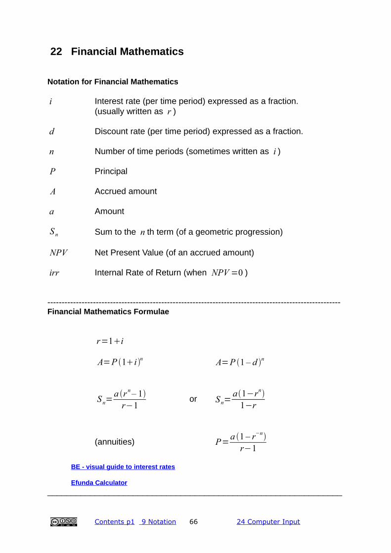
22 Financial Mathematics
Notation for Financial Mathematics
i Interest rate (per time period) expressed as a fraction. (usually written as r )
d Discount rate (per time period) expressed as a fraction.
n Number of time periods (sometimes written as i )
P Principal
A Accrued amount
a Amount
S n Sum to the n th term (of a geometric progression)
NPV Net Present Value (of an accrued amount)
irr Internal Rate of Return (when NPV=0 )
-------------------------------------------------------------------------------------------------------Financial Mathematics Formulae
r=1i
A=P 1i n A=P 1 – d n
S n=a r n – 1
r−1or S n=
a1−rn
1−r
(annuities) P=a 1 – r−n
r−1
BE - visual guide to interest rates
Efunda Calculator
______________________________________________________________
Contents p1 9 Notation 66 24 Computer Input

23 Recommended Computer Programs
wxMaxima free (Open Source) MS Windows and Linux
http://wxmaxima.sourceforge.net/wiki/index.php/Main_PageWindows: download maxima 5.24.0 (or later version)
http://portableapps.com/node/18166 (portable application)
A open source free download computer algebra system. It is being constantly updated. You are not allowed implicit multiplication.
5e 2t3sin 4 typed as 5∗% e ^ 2∗t 3∗sin % pi/4
The % sign designates special functions. (numerical values of letters)
Maxima is a system for the manipulation of symbolic and numerical expressions, including differentiation, integration, Taylor series, Laplace transforms and ordinary differential equations. Also, Maxima can plot functionsand data in two and three dimensions.
-----------------------------------------------------------------------------------------------Geogebra free (Open Source) MS Windows and Linux
http://www.geogebra.org
This program can be accessed over the web i.e. you do not need to download it although you need to be running Java Runtime Environment (free download). GeoGebra is a dynamic mathematics software that joins geometry,algebra and calculus. An expression in the algebra window corresponds to an object in the geometry window and vice versa.----------------------------------------------------------------------------------------------------Mathcad ( £1000 approx.) MS WindowsThis is the tool of choice for most engineering mathematics. Notes available.Mathcad Notes
---------------------------------------------------------------------------------------------------SMath free (Closed Source) MS Windows and Linux
http://en.smath.info/forum/default.aspx?g=posts&t=1158Looks and works like Mathcad. Notes here SMath Primer
---------------------------------------------------------------------------------------------------Graph free (Open Source) MS WindowsA useful graphing tool which is easy to use. http://www.padowan.dk/graph/
---------------------------------------------------------------------------------------------------Casio Calculator Manuals (in pdf format)
http://support.casio.com/manual.php?rgn=2&cid=004_______________________________________________________________________
Contents p1 9 Notation 67 24 Computer Input

24 Computer Input
wxMaxima and Geogebra are recommended . Most of this also applies to spreadsheets and online maths sites. Spreadsheet programs are not recommended (except for statistical calculations).
Calculator keyComputer (Keyboard) entry
Geogebra (3) Mathcad (2) wxMaxima (5)× ∗ ∗ (Shift 8) ∗÷ / / /
x 2 ^2^2
(Shift 6 then 2)^2
(Shift 6 then 2)x▄ or ^ or x y
or y x ^ ^ ^
sqrt() (also ondrop down list)
\ sqrt( )
x ^1x
nCalculator toolbar
^1x
5sin xo30o(1)
5sin xo30oo symbol fromdrop down list
5sin x deg30 deg 5*sin(x/180*%pi+30/180*%pi)
e xe from drop
down list then ^or exp( )
e x%e^( )
orexp( )
ln ln ln logπ pi CTRL g %pi
10××0.7 10 pi *0.7 10 CTRL g*0.7 10*%pi*0.7
sin−10.5means
arcsin(0.5)asin(0.5) asin(0.5) asin(0.5)
(1) As all programs work in radians by default you must change every input into degrees (if you have to work in degrees).
(2) Also available on toolbars.(3) Only x allowed as variable(4) See also 17.5
(5) In wxMaxima typing pi will produce π as a variable NOT 3.1415...The same is true for e .
Back to 2 Web Sites ------------------------------------------------------------------------------------------------------
Contents p1 9 Notation 68 24 Computer Input

24.1 wxMaxima InputNote: From version 0.8.1 use Shift+Enter to enter expressions
to change behaviour go to Edit: Configure
See wxMaxima Introduction at Notes and exercises See http://www.math.hawaii.edu/~aaronts/maximatutorial.pdf a simple introduction.See http://www.neng.usu.edu/cee/faculty/gurro/Maxima.html but put in expression first!and Maxima by Example http://www.csulb.edu/~woollett/ ------------------------------------------------------------------------------------------------Note: Implicit multiplication is NOT allowed. 3 x is always typed as 3∗x--------------------------------------------------------------------------------------------------------Zoom in Alt I Insert Text Box CTRL 1 (or F6)Zoom out Alt O------------------------------------------------------------------------------------------------Copy as an Image to a Edit - Select AllSpreadsheet File Right click – Copy as Image...
Paste onto a worksheet------------------------------------------------------------------------------------------------------Assign w:3.7 (means w=3.7 ) f(x):=3*x (means f x =3x )-------------------------------------------------------------------------------------------------------
Matrix multiplication [ ]⋅[ ] Use . Do not use ∗
-------------------------------------------------------------------------------------------------------Newton Raphson
load(newton1)
newton f x , x , x0, p . Start with precision p=0.1 and thenp=0.01 etc. until outputs are identical to
significant figures required- - - - - - - - - - - - - - - - - - - - - - - - - - - - - - - - - - - - - - - - - - - - - - - - - - - - - - - - - 24.1.1 Differential Equations
see also 20.4 (2nd page)dydx
typed as ‘diff(y,x) note the apostrophe ‘ before diff
d 2 y
d x 2 typed as ‘diff(y,x,2)
Equations; Solve ODE. Equations; Initial value problem (1) or (2).- - - - - - - - - - - - - - - - - - - - - - - - - - - - - - - - - - - - - - - - - - - - - - - - - - - - - - - - - 24.1.2 Runge-Kutta
rk f x , y , y , y0, [ x , x0, xend , h] where dydx= f (x , y) 20.5
To plot result: wxplot2d([discrete,%o#],[style,points])you can replace points with line. %o# is a previous output line.
-------------------------------------------------------------------------------------------------------
Contents p1 9 Notation 69 24 Computer Input

24.2 Mathcad Input
Applied MathsDefinition of variables and functionsvariable := number and units (:= use colon :)
Example: x:3kg will read as x :=3 kg and a:5 m/s^2 as a :=5 ms2
Function f x := function in terms of x Example: f(x): x*a will be interpreted as f x :=x⋅a
= gives numerical answer Example f x = will produce the answer 15 N ▄You can type a different unit in place of the box and the number will change to satisfy the units chosen.- - - - - - - - - - - - - - - - - - - - - - - - - - - - - - - - - - - - - - - - - - - - - - - - - - - - - - - - -Symbolic Maths
f x = use Boolean (bold) equals symbolic units
Implicit multiplication: This is allowed but only with variables that cannot be confused with units.For example, 3 x is fine but 3 s must be typed as 3∗s .When editing expressions use the Ins key to change from editing to the left to editing to the right of cursor.
Also see Mathcad Notes_____________________________________________________________ 24.3 SMath
This entry will be expanded but at the moment have a look at the SMath Primer by Bernard V Liengme http://people.stfx.ca/bliengme/SMath/SmathPrimer.pdf
This is a truly remarkable program that looks and works like Mathcad and should be of use to engineers in particular. It is also available as a live program - no download required although that particular version may have a few bugs.
Contents p1 9 Notation 70 24 Computer Input
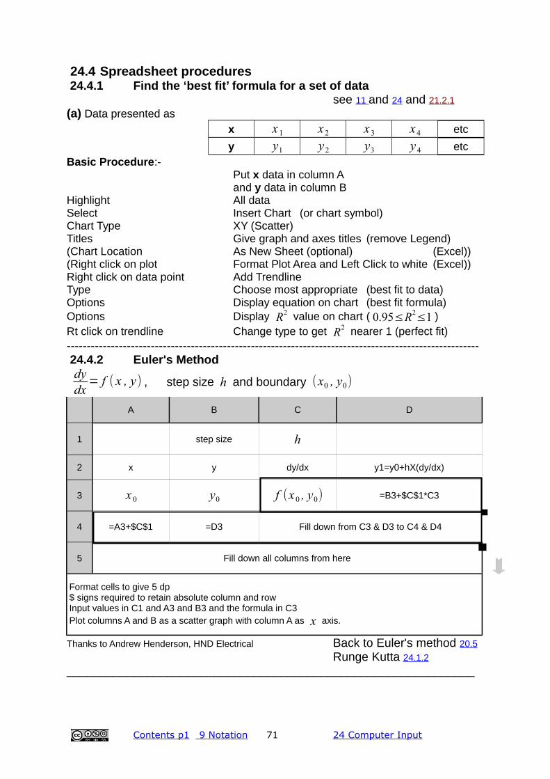
24.4 Spreadsheet procedures 24.4.1 Find the ‘best fit’ formula for a set of data
see 11 and 24 and 21.2.1
(a) Data presented as
x x 1 x 2 x 3 x 4 etc
y y1 y2 y3 y 4 etcBasic Procedure:-
Put x data in column A and y data in column B
Highlight All dataSelect Insert Chart (or chart symbol)Chart Type XY (Scatter)Titles Give graph and axes titles (remove Legend)(Chart Location As New Sheet (optional) (Excel))(Right click on plot Format Plot Area and Left Click to white (Excel))Right click on data point Add TrendlineType Choose most appropriate (best fit to data)Options Display equation on chart (best fit formula)Options Display R2 value on chart ( 0.95≤R2
≤1 )Rt click on trendline Change type to get R2 nearer 1 (perfect fit)------------------------------------------------------------------------------------------------------- 24.4.2 Euler's Method
dydx= f ( x , y) , step size h and boundary (x0 , y0)
A B C D
1 step size h
2 x y dy/dx y1=y0+hX(dy/dx)
3 x 0 y0 f (x 0 , y0) =B3+$C$1*C3
4 =A3+$C$1 =D3 Fill down from C3 & D3 to C4 & D4
5 Fill down all columns from here
Format cells to give 5 dp$ signs required to retain absolute column and rowInput values in C1 and A3 and B3 and the formula in C3Plot columns A and B as a scatter graph with column A as x axis.
Thanks to Andrew Henderson, HND Electrical Back to Euler's method 20.5
Runge Kutta 24.1.2
_____________________________________________________________
Contents p1 9 Notation 71 24 Computer Input

This page is intentionally not blank
Contents p1 9 Notation 72 24 Computer Input

This page is intentionally not blank
Contents p1 9 Notation 73 24 Computer Input

25 Calibration Error
-------------------------------------------------------------------------------------------------------Thanks to Olaniyi Olaosebikan, Aberdeen College
PIDProportional/Integral/Differential Control: See http://dexautomation.com/pidtutorial.php
Measurement and UncertaintyNational Physical Laboratory. See: http://www.npl.co.uk/publications/uncertainty-guide/uncertainty-of-measurement-guides
UKAS M3003 http://www.ukas.com/library/Technical-Information/Pubs-Technical-Articles/Pubs-List/M3003.pdf
Contents p1 9 Notation 74 24 Computer Input
Input
Output
IDEALInput = Output
Input
Output
Zero Error
Input
Output
Span Error
Input
Output
Linearity ErrorFirst and Last Values coincide
Input
Output
Zero-Span Error
Input
Output
Linearity ErrorFirst and Last Values coincide

26 Mechanical Tables
26.1.1 Properties of Materials
Material Melting point oC Density kg/m3 Notes
Water (Fresh) (H2O) 0 1000at Standard Temperature and
Pressure
Plastics 850 - 1400for PETE/ PVC, polypropylene
Aluminium (Al) 660 2700 at STPSteel (Fe+C) 1525-1540 7850 at STPCopper (Cu) 1085 8920 - 8960 at room tempSilver (Ag) 962 10500 at STPLead (Pb) 327 11340 at room temp
Mercury (Hg) -39 13546 at STPTungsten (W) 3422 19300 at STP
Gold (Au) 1064 19320 at STPhttp://en.wikipedia.org/wiki/Densityhttp://en.wikipedia.org/wiki/Melting_points_of_the_elements_%28data_page%29
26.1.2 Young's Modulus- approximate.
Material Young's Modulus GN/m2
Rubber 0.01 – 0.1HDPE 0.8Nylon 2 - 4MDF 4
High strength concrete under compression 30Aluminium 69
Glass 50 - 90Brass / Bronze 100 - 125Titanium alloy 105 - 120
Carbon Fibre reinforced plastic (70/30) 181Steel 200
Silicon Carbide 450Tungsten Carbide 450 - 650
Single-walled carbon nanotube 1000+Diamond 1220
http://en.wikipedia.org/wiki/Young%27s_modulus
Contents p1 9 Notation 75 24 Computer Input

27 Periodic Table of The Elements1A 2A 3A 4A 5A 6A 7A 8A
11H
1.008Hydrogen
3B 4B 5B 6B 7B 8B 8B 8B 1B 2B 2He
4.003Helium
23Li
6.941Lithium
4Be
9.012Beryllium
See the Periodic Table of Videos at http://www.periodicvideos.com/5B
10.81Boron
6C
12.01Carbon
7N
14.01Nitrogen
8O
16.00Oxygen
9F
19.00Fluorine
10Ne
20.18Neon
311Na
22.99Sodium
12Mg
24.31Magnesium
13Al
26.98Aluminium
14Si
28.09Silicon
15P
30.97Phosphorus
16S
32.07Sulphur
17Cl
35.45Chlorine
18Ar
39.95Argon
419K
39.10Potassium
20Ca
40.08Calcium
21Sc
44.96Scandium
22Ti
47.88Titanium
23V
50.94Vanadium
24Cr
52.00Chromium
25Mn
54.94Manganese
26Fe
55.85Iron
27Co
58.93Cobalt
28Ni
58.69Nickel
29Cu
63.55Copper
30Zn
65.39Zinc
31Ga
69.72Gallium
32Ge
72.61Germanium
33As
74.92Arsenic
34Se
78.96Selenium
35Br
79.90Bromine
36Kr
83.80Krypton
537Rb
85.47Rubidium
38Sr
87.62Strontium
39Y
88.91Yttrium
40Zr
91.22Zirconium
41Nb
92.91Niobium
42Mo
95.94Molybdenum
43Tc
(98)Technetium
44Ru
101.1Ruthenium
45Rh
102.9Rhodium
46Pd
106.4Palladium
47Ag
107.9Silver
48Cd
112.4Cadmium
49In
114.8Indium
50Sn
118.7Tin
51Sb
121.8Antimony
52Te
127.6Tellurium
53I
126.9Iodine
54Xe
131.3Xenon
655Cs
132.9Caesium
56Ba
137.3Barium
*57La
138.9Lanthanum
72Hf
178.5Hafnium
73Ta
180.9Tantalum
74W
183.9Tungsten
75Re
186.2Rhenium
76Os
190.2Osmium
77Ir
192.2Iridium
78Pt
195.1Platinum
79Au
197.0Gold
80Hg
200.6Mercury
81Tl
204.4Thallium
82Pb
207.2Lead
83Bi
209.0Bismuth
84Po
(209)Polonium
85At
(210)Astatine
86Rn
(222)Radon
787Fr
(223)Francium
88Ra
226.0Radium
**89Ac
227.0Actinium
104Rf
(261)Ruther-fordium
105Db
(262)Dubnium
106Sg
(263)Seaborgium
107Bh
(262)Bohrium
108Hs
(265)Hassium
109Mt
(268)Meitner-
ium
110Ds
(269)Darm-
stadtium
111Rg
(272)Roentgen
-ium
112Cn
(277)Copernic-
ium
113Uut
(284)Ununtrium
114Fl
(283)Flerovium
115Uup(288)
Ununpent-ium
116Lv
(289)Livermor-
ium
117Uus(293)
Ununsept-ium
118Uuo(294)
Ununoct-ium
* LanthanideSeries
58Ce
140.1Cerium
59Pr
140.9Praseo-dymium
60Nd
144.2Neodymium
61Pm
(145)Promethium
62Sm
150.4Samarium
63Eu
152.0Europium
64Gd
157.3Gadolinium
65Tb
158.9Terbium
66Dy
162.5Dysprosium
67Ho
164.9Holmium
68Er
167.3Erbium
69Tm
168.9Thulium
70Yb
173.0Ytterbium
71Lu
175.0Lutetium
** ActinideSeries
90Th
232.0Thorium
91Pa
231.0Protactinium
92U
238.0Uranium
93Np
237.0Neptunium
94Pu
(244)Plutonium
95Am
(243)Americium
96Cm
(247)Curium
97Bk
(247)Berkelium
98Cf
(251)Californium
99Es
(252)Einsteinium
100Fm
(257)Fermium
101Md
(258)Mendelevium
102No
(259)Nobelium
103Lr
(260)Lawrencium
Based on: Cracolice & Peters, Introductory Chemistry, 2/e, 2004. Thanks to a student for starting this, Fall 1997.*** or mass number of most common, most stable, or first-discovered isotope.Reproduced by permission of Bob Bruner http://bbruner.org/ June 2, 2012
Contents p1 9 Notation 76 24 Computer Input
KEY Atomic number 1 Symbol H Atomic mass *** 1.008 Name of the element Hydrogen

SI Units - Commonly used prefixesmeaning multiple prefix symbol
×1000000000000000 ×1015 Peta P
×1000000000000 ×1012 Tera T
×1000000000 ×109 Giga G
×1000000 ×106 Mega M
×1000 ×103 kilo k
×1 ×100
÷1000 ×10−3 milli m
÷1000000 ×10−6 micro
÷1000000000 ×10−9 nano n
÷1000000000000 ×10−12 pico p
28 Electrical Tables
Table of Resistivities Relative Static Permittivity
MaterialResistivity m at 20o C
MaterialDielectric Constant r
Silver (Ag) 15.9×10⁻⁹ Vacuum 1Copper (Cu) 17.2×10⁻⁹ Air 1.00054Gold (Au) 24.4×10⁻⁹ Diamond (C) 5.5 - 10Tungsten (W) 56.0×10⁻⁹ Salt (NaCl) 3 - 15Nickel (Ni) 69.9×10⁻⁹ Graphite (C) 10 - 15Iron (Fe) 100×10−9 Silicon (Si) 11.68Lead (Pb) 220×10−9
Carbon (C) 35000×10−9
Permeability Values for some Common Materials
MaterialPermeability (H/m)
Electrical Steel 5000×10−6 Ferrite (Nickel Zinc) (Ni Zn) 20 – 800×10−6
Ferrite (Manganese Zinc) (Mn Zn) 800×10−6
Steel 875×10−6
Nickel (Ni) 125×10−6
Aluminium (Al) 1.26×10⁻⁶
Thanks to Satej Shirodkar, Aberdeen College.
Contents p1 9 Notation 77 24 Computer Input

29 THE GREEK ALPHABET
UPPER lower CASE case Pronunciation Examples of use
A Alpha angles, angular acceleration
B Beta angles
Gamma shear strain, heat capacity, kinematic viscosity
Delta DIFFERENTIAL, the change in... (Calculus)
E Epsilon linear strain, permittivity
Z Zeta impedance, damping ratio
H Eta efficiency, viscosity
Theta angles, temperature, volume strain
I Iota inertia
K Kappa compressibility
Lambda wavelength, thermal conductivity, eigenvalues
M Mu micro (10-6 ), coefficient of friction
N Nu velocity
Xi damping coefficient
O Omicron
Pi PRODUCT, 3.141592654...., C= d
P Rho density, resistivity
Sigma SUM; standard deviation, normal stress
T Tau shear stress, torque, time constant
Upsilon admittance
Phi angles, flux, potential energy, golden ratio
X Chi PEARSON’S 2 TEST , angles
Psi helix angle (gears), phase difference
Omega RESISTANCE; angular velocity
_____________________________________________________________
This work, to be attributed to Peter K Nicol, Aberdeen College is licensed
under the Creative Commons Attribution-NonCommercial-ShareAlike 3.0
Unported License. To view a copy of this license, visit
http://creativecommons.org/licenses/by-nc-sa/3.0/ (click on icon below) or
send a letter to Creative Commons, 171 Second Street, Suite 300, San
Francisco, California, 94105, USA.
Contents p1 9 Notation 78 24 Computer Input


![HANDBOOK FORMULA BOOK - Engineers Institute FORMULA BOOK 1. NETWORK THEORY [4] Published by: ENGINEERS INSTITUTE OF INDIA. ALL RIGHTS RESERVED Transformer doesn’t work as amplifier](https://static.fdocuments.net/doc/165x107/5ad0b8da7f8b9a1d328ea104/handbook-formula-book-engineers-institute-formula-book-1-network-theory-4-published.jpg)