Formation control in environment with dynamic obstacles...

CZECH TECHNICAL UNIVERSITY IN PRAGUE

Faculty of Electrical Engineering

BACHELOR THESIS

Filip Eckstein

Formation control in environment with dynamicobstacles

Department of Cybernetics

Thesis supervisor: Dr. Martin Saska

Statement

I hereby declare that I have completed this thesis independently and that I have usedonly the sources (literature, software, etc.) listed in the enclosed bibliography.I have no objection to usage of this work in compliance with the act §60 Zakon c. 121/2000Sb.(copyright law), and with the rights connected with the copyright act including the changesin the act.

In Prague on............................. ...............................................

Acknowledgment

Foremost, I would like to thank to Ing. Martin Saska Dr. rer. nat. for his excellentsupervision and relevant discussions. I would also like to thank to Ing. Jan Chudoba fora great technical support during the SyRoTek experiments and to Mgr. Dan Erben MResfor critical evaluation of this thesis. Great gratitude also goes to my family for calm andpatient environment they provided me during the study.

Formation control in environment with dynamic obstacles

Abstract

Trajectory planning of nonholonomic formations of mobile robots is achallenging problem in mobile robotics. It enables robotic formations toautonomously move in static and also dynamic environment. The aim ofthis thesis is to study formation control in environment with dynamic ob-stacles and integrate dynamic obstacle avoidance algorithm into rules ofMPC (Model-predictive control) using framework that is being developedat Department of Cybernetics, CTU in Prague. The final verification ofthe complete system has been simulated by a movement of formation ina real experiment with the SyRoTek system.


Abstrakt

Planovanı trajektoriı formacı mobilnıch robotu patrı v mobilnı roboticek podnetnym problemum predstavujıcıch dulezitou soucast budoucıhorozvoje robotickych aplikacı. Robotickym formacım umoznuje au-tonomnı pohyb nejen ve statickem, ale i v dynamickem prostredı. Cılemteto bakalarske prace je podrobne prostudovanı teorie rızenı formacıv dynamickem prostrednı a integrace vhodnych pravidel umoznujıcıchrobotickym formacım vyhybat se dynamickym prekazkam. Prace sezaklada na rozsırenı projektu vyvıjenym katedrou Kybernetiky CVUTv Praze. Overenı funkcnosti vysledneho systemu probehne na realneroboticke platforme SyRoTek.

CONTENTS Formation control in environment with dynamic obstacles

Contents

1 Introduction 1

1.1 Motivation . . . . . . . . . . . . . . . . . . . . . . . . . . . . . . . . . . . . 1

1.1.1 Leader-follower approach . . . . . . . . . . . . . . . . . . . . . . . . 1

1.1.2 Practical use . . . . . . . . . . . . . . . . . . . . . . . . . . . . . . 1

1.1.3 Contributions . . . . . . . . . . . . . . . . . . . . . . . . . . . . . . 2

1.2 State of the art . . . . . . . . . . . . . . . . . . . . . . . . . . . . . . . . . 2

1.3 Model details . . . . . . . . . . . . . . . . . . . . . . . . . . . . . . . . . . 4

1.4 Car-like robot . . . . . . . . . . . . . . . . . . . . . . . . . . . . . . . . . . 5

2 Implementation 6

2.1 Initialization trajectory . . . . . . . . . . . . . . . . . . . . . . . . . . . . . 6

2.1.1 Visibility graph . . . . . . . . . . . . . . . . . . . . . . . . . . . . . 6

2.2 Model predictive control . . . . . . . . . . . . . . . . . . . . . . . . . . . . 9

2.2.1 Robot’s configuration space . . . . . . . . . . . . . . . . . . . . . . 9

2.2.2 Kinematics and model . . . . . . . . . . . . . . . . . . . . . . . . . 9

2.2.3 Constraints . . . . . . . . . . . . . . . . . . . . . . . . . . . . . . . 10

2.2.4 Shape of a formation . . . . . . . . . . . . . . . . . . . . . . . . . . 10

2.2.5 The cost function . . . . . . . . . . . . . . . . . . . . . . . . . . . . 11

2.3 Implemented models . . . . . . . . . . . . . . . . . . . . . . . . . . . . . . 11

2.3.1 Rules extension for dynamic obstacles . . . . . . . . . . . . . . . . . 11

2.3.2 Linear model interpretation . . . . . . . . . . . . . . . . . . . . . . 12

2.3.3 Quadratic model interpretation . . . . . . . . . . . . . . . . . . . . 13

2.3.4 Implementation details . . . . . . . . . . . . . . . . . . . . . . . . . 13

2.4 Complicated maneuvers . . . . . . . . . . . . . . . . . . . . . . . . . . . . 15

2.4.1 Flow chart . . . . . . . . . . . . . . . . . . . . . . . . . . . . . . . . 16

3 Simulations and results 17

3.1 Computer simulations . . . . . . . . . . . . . . . . . . . . . . . . . . . . . 17

3.1.1 Linear model . . . . . . . . . . . . . . . . . . . . . . . . . . . . . . 17

3.1.2 Quadratic model . . . . . . . . . . . . . . . . . . . . . . . . . . . . 20

3.2 Quality of solution . . . . . . . . . . . . . . . . . . . . . . . . . . . . . . . 20

i

CONTENTS Formation control in environment with dynamic obstacles

3.3 Results and graphs . . . . . . . . . . . . . . . . . . . . . . . . . . . . . . . 22

3.3.1 Static vs. linear model . . . . . . . . . . . . . . . . . . . . . . . . . 22

3.3.2 All models comparison . . . . . . . . . . . . . . . . . . . . . . . . . 23

4 Experiments with SyRoTek 25

4.1 About SyRoTek . . . . . . . . . . . . . . . . . . . . . . . . . . . . . . . . . 25

4.2 Computer simulation . . . . . . . . . . . . . . . . . . . . . . . . . . . . . . 26

4.3 Experiments . . . . . . . . . . . . . . . . . . . . . . . . . . . . . . . . . . . 28

4.3.1 Initialization conditions . . . . . . . . . . . . . . . . . . . . . . . . 28

4.3.2 Implementation details . . . . . . . . . . . . . . . . . . . . . . . . . 28

4.3.3 Mission . . . . . . . . . . . . . . . . . . . . . . . . . . . . . . . . . 28

4.4 Experiences with system . . . . . . . . . . . . . . . . . . . . . . . . . . . . 30

4.4.1 Recommendations . . . . . . . . . . . . . . . . . . . . . . . . . . . . 30

4.4.2 Brief summary of recommendations . . . . . . . . . . . . . . . . . . 31

5 Conclusion 32

5.1 Future of the project . . . . . . . . . . . . . . . . . . . . . . . . . . . . . . 32

6 Appendix A 33

6.1 Tables of results . . . . . . . . . . . . . . . . . . . . . . . . . . . . . . . . . 33

7 Appendix B 36

ii

LIST OF FIGURES Formation control in environment with dynamic obstacles

List of Figures

1 Real indoor experiment of robot plow formation developed by Intelligentand Mobile Robotics Group, CTU in Prague. . . . . . . . . . . . . . . . . . 2

2 Demonstration of predictive model approach . . . . . . . . . . . . . . . . . 4

3 The approximate chart of application modules of model predictive control.The rules extension, which is the main purpose of this thesis, is marked byred bubble. . . . . . . . . . . . . . . . . . . . . . . . . . . . . . . . . . . . 7

4 Computer simulation of visibility graph with dijkstra shortest path searchingalgorithm. . . . . . . . . . . . . . . . . . . . . . . . . . . . . . . . . . . . . 8

5 The demonstration of measuring Euclidean distance between marauder andleader. . . . . . . . . . . . . . . . . . . . . . . . . . . . . . . . . . . . . . . 15

6 Flowchart of the algorithm which is responsible for avoiding collisions innon-predicated situations. . . . . . . . . . . . . . . . . . . . . . . . . . . . 16

7 Computer demonstration of a feasible solution solved by linear model ofextended rules of model predictive control. . . . . . . . . . . . . . . . . . . 18

8 Computer demonstration of a feasible solution solved by quadratic model ofextended rules of model predictive control. . . . . . . . . . . . . . . . . . . 19

9 Comparison between linear and quadratic solver for the same initializationconditions. . . . . . . . . . . . . . . . . . . . . . . . . . . . . . . . . . . . . 20

10 Demonstration of collision state of a badly tuned predictive model. . . . . 21

11 Graphic comparison of static and linear model for linear movement of thedynamic obstacle (in sense of final time). . . . . . . . . . . . . . . . . . . . 23

12 Graphic comparison of static and linear model for linear movement of thedynamic obstacle (in sense of minimal distance to collision). . . . . . . . . 23

13 Graphic comparison of all models for quadratic movement of the dynamicobstacle (in sense of final time). . . . . . . . . . . . . . . . . . . . . . . . . 24

14 Graphic comparison of all models for quadratic movement of the dynamicobstacle (in sense of minimal distance to collision). . . . . . . . . . . . . . 24

15 One of twelve robots, that are forming an active part of a SyRoTek roboticsystem. . . . . . . . . . . . . . . . . . . . . . . . . . . . . . . . . . . . . . . 25

16 Communication scheme of the SyRoTek system. . . . . . . . . . . . . . . . 26

17 Computer simulation of experiment in the SyRoTek system arena . . . . . 27

18 Camera record of SyRoTek system during the experiment. . . . . . . . . . 29

19 Camera record of SyRoTek system during the experiment. . . . . . . . . . 29

iii

LIST OF TABLES Formation control in environment with dynamic obstacles

List of Tables

1 Comparison of final times of all implemented models . . . . . . . . . . . . 33

2 Comparison of minimal distances to collision of all models . . . . . . . . . 34

3 Linear movement of dynamic obstacle, comparison of final time and minimaldistance to collision . . . . . . . . . . . . . . . . . . . . . . . . . . . . . . . 35

4 CD Content . . . . . . . . . . . . . . . . . . . . . . . . . . . . . . . . . . . 36

iv

LIST OF SCENARIOS Formation control in environment with dynamic obstacles

List of scenarios

1 The algorithm for trajectory planning using MPC approach with new rulesfor avoiding dynamic obstacles implemented. . . . . . . . . . . . . . . . . . 14

v


1 Introduction

The main goal of this thesis is an integration, simulation and final verification of theextension of the model predictive control (MPC)1 focused algorithms to avoid obstacles indynamic environment in experiments with car-like2 robots according to certain models.

These algorithms will be integrated into rules of the formation control (Section 2.2). Theintegration of new models of dynamic obstacle avoidance methods consists in design andimplementation of an ability to predict a movement of dynamic obstacles that improvesthe final solution of the robot solver (Section 2.3). The quality of the predetermined modelof dynamic obstacle represents a significant influence on the feasibility of the final solution.This work using a model predictive control based theory which is being developed by theDepartment of Cybernetics, CTU in Prague.

1.1 Motivation

1.1.1 Leader-follower approach

This work is based on the leader-follower approach. In practice, this means that oneor more robots are designed to be leaders, and their states are distributed within therest of formation. The followers are designed to maintain positions relative to the state ofthe leaders. The utilization of this approach is motivated by heterogeneity of the roboticformation, because it allows to well equip (with additional sensors, computing power etc.)only robots that are determined to be leaders. The rest of robots from the formation(followers) can be simpler and the only technology they must carry are drive and wirelessdevices to communication with the leader.

1.1.2 Practical use

The purpose of this thesis is to simulate and test on a real robotic platform new imple-mented rules of model predictive control for trajectory planning. In practice, this approachcan be used for many applications nowadays or in the future, because the need for flexibleautonomous robots for working in dynamic workspace is still rising. One of the most re-vealing example in the future can be snow removal from airports (as was showed in [1]) asbeing one of the target applications of this approach. The network of runways and airportcorridors is a fine example of a vast space dynamic environment, where adaptable forma-tion of autonomous robots can be used. Main advantage of using robotic formations liewithin an energetic effectivity caused by planning of an optimal cleaning trajectory thatcan much more easily predetermine a behavior of dynamic obstacles3 and convert them to

1Model predictive control theory will be explained in Section 2.2.2Car-like robot will be described in more detail in Section 2.2.23In this case cars, planes, etc.

1/37

1.2 State of the art Formation control in environment with dynamic obstacles

a mathematical model. Optimal trajectory planning in combination with predictive modelsof dynamic objects can lower the amount of consumed fuel and save time.

Figure 1: Real indoor experiment of robot plow formation developed by Intelligent andMobile Robotics Group, CTU in Prague.

1.1.3 Contributions

The main contribution of this project lies within the extension of the MPC frameworkbeing developed at the Department of Cybernetics, CTU in Prague. Testing the overallMPC system and its simulation on the real multi-robotic platform4 brought a significantprogress in development of real time planning algorithms. A demonstration of the realtime online computation of the MPC system on the SyRoTek platform was executed asthe first experiment of this kind. Up to now, only the offline version of this approachwas tested as is shown in the Figure 1. Implementation and comparison of two predictivemodels also verified the functionality and usefulness in the real application domains, wherethe environment consists of dynamic obstacles, where model of movement can be easilypredetermined.

1.2 State of the art

Navigation based functions and motion planning of car-like robots formations draws agreat deal of interest in mobile robotics. A several methodologies and formulations of con-trolling multi-agent system to reach the target position in dynamic environment with min-imum time and the highest possible robustness in the sense of avoiding collisions whetherwith obstacles or with other members of the formation has been formed. Among the main

4Experiment with the SyRoTek system will be explained in more detail in Section 4

2/37

1.2 State of the art Formation control in environment with dynamic obstacles

approaches which we will devote this chapter belongs the Receding Horizon Control (pre-sented by Saska, Mejıa, Stipanovic and Schilling in 2009 [2] and Dunbar and Murray in2004 [3]) and an example of decentralized concept of Collision Avoidance Scheme for Mul-tiple Independent Non-point Agents (presented by Dimarogonas, Loizou, Kyriakopoulosand Zavlanos in 2005 [4].In this thesis, we will present a predictive collision avoidance extension of model predictivecontrol approach, but we will also introduce a different point of view in the sense of statespace motion planning algorithms with solving the collision scenarios.

The main difference between centralized and decentralized (as was described in [4] con-cept lies in the knowledge of target region, which is supposed to be reached by othermembers of the formation. Decentralized method considers a multi-agent formation, whereeach agent has knowledge only of its own desired destination but not of the others [4], whilecentralized concept is supposed to (leader-follower approach5) share the actual state of therobot leader within the rest of the formation to follow it. It means that the goal region isthe same for all the members of the formation. To demonstrate the advantages of decen-tralized approach, a basic motivation of decentralized method was introduced in [4] andcomes from practical application domain, where implemented navigation functions pro-vide increased robustness in the sense of agent failures. This advantage makes the methodappropriate for conflict resolutions in air traffic management. According to Dimarogonas,Loizou, Kyriakopoulos and Zavlanos, reduced computational complexity makes the de-centralized approach more appealing to centralized ones. Due to simulations of CollisionAvoidance Scheme for Multiple Independent Non-point Agents presented in [4], each agentis forced to participate in the conflict resolution procedure even if already in its final des-tination region. But the decentralized method of navigation of a formations (consisted ofcar-like robots) is not the only matter of highly critical application such as air traffic con-trol. Jaeger and Nebel in the Dynamic Decentralized Area Partitioning for CooperatingCleaning Robots [6] used this approach for cooperative cleaning of a large room withoutglobal synchronization or global communication network.

Another area of interest, where the robot motion planning can bring a significant im-provement can be for example the mapping of hazardous areas (as was described in [7]),where an appropriate sensor equipment can track sources of environmental or biologicalradiation using Particle Swarm Optimization algorithms (PSO). There are also other in-teresting applications and methods such as trajectory planning through neural networksand genetic algorithm as is shown in A neural network approach to complete coverage pathplanning from 2004 [8].

Motion and trajectory planning in the multi-robotic system can be interpreted by severalmethods and as is shown in the last subsection, it is important to choose an appropriateapproach for the most feasible solution of desired mission of our multi-agent robotic system.For purpose of this thesis, we have chosen a model predictive control for driving multi-

5The leader-follower approach was also used by Fierro, Das, Kumar and Ostrowski in the Hybrid Controlof Formations of Robots from 2001 [5].

3/37

1.3 Model details Formation control in environment with dynamic obstacles

robotic formations.

1.3 Model details

Concept of model predictive approach can be interpreted as a predictive informationof obstacle’s next movement. In practice we can imagine this problem as two cars at anintersection. Driver in the first car observes other car that is moving at the crossroadsaccording to a certain model. For instance, second car has constant velocity and zerocurvature, so the direction does not fluctuate. Based on this approximate model, driverof the first car can predetermine where the second car on the crossroads will be in nextseconds and is able to avoid a collision.

Figure 2: Demonstration of predictive model approach

In this thesis we will be using two types of models of dynamic obstacles: linear andquadratic. These two models are defined by the change of position over time (velocity)and curvature. The properties of the linear model rest in constant velocity and zero curva-ture while quadratic model is defined by velocity and non-zero curvature. If velocity andcurvature are not defined, we will consider the model as static.

4/37

1.4 Car-like robot Formation control in environment with dynamic obstacles

1.4 Car-like robot

We can describe a car-like robot concept as a vehicle with four wheels, where the frontpair of wheels is able to change angle. In combination with forward velocity, a robotcan change a heading like a four-wheeled car. Kinematic model of car-like robot will bedescribed in more detail in Section (2.2.2).In hardware experiments with the SyRoTek system, substitution of four-wheeled car-likerobot for a robot with two actuated wheels will be necessary. Because of this, the change ofheading will be converted from angle in radians to the input angular velocity. Experimentswith the SyRoTek system will be discussed in Section (4).

5/37


2 Implementation

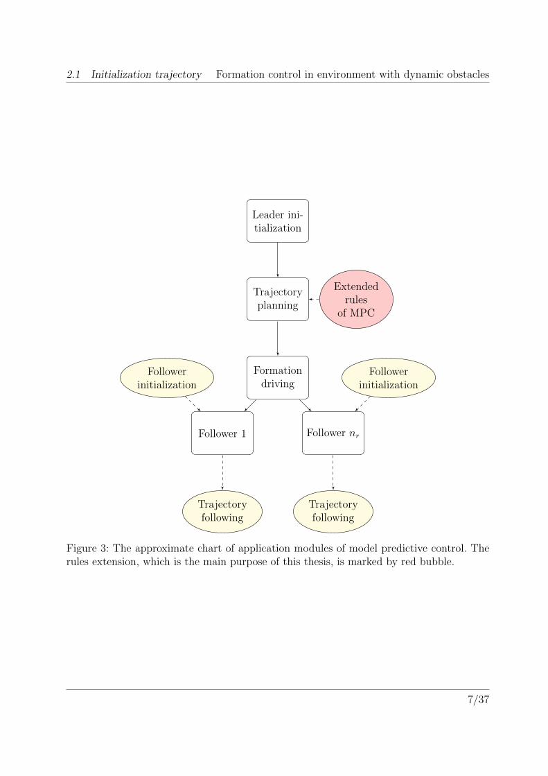
Control and navigation algorithms of formations of car-like robots are not the primarysubject of this thesis but it represents the key part by providing a core framework forthis project. Brief description of this approach will be described in section (2.2). Detailedexplanation of MPC implementation can be found in [1]. The approximate chart is shownin Figure (3).

2.1 Initialization trajectory

Model predictive control as utilized in this thesis works on basis of pushing and op-timizing known control points of input predetermined trajectory. This trajectory, whichis defined by user or state space searching computer algorithm (RRT6, visibility graph,Voronoi diagram etc.), need not to be necessarily optimal but it should provide the mostfeasible solution possible. Imperfection of input trajectory in sense of colliding with wallsor other obstacles can cause high amount of local minima in the cost function7. Then theprocess can easily get stuck and robot will not find feasible solution.

2.1.1 Visibility graph

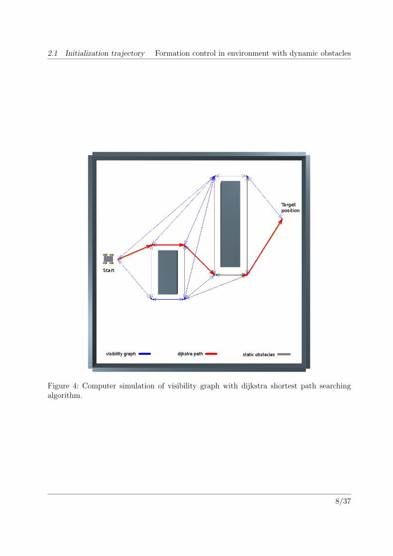
For needs of this project (in sense of initialization trajectory as an input of the optimiza-tion), the visibility graph algorithm was chosen. In definition, in robot motion planning, avisibility graph is a graph typically consisted of nodes and edges in the Euclidean plane.Locations of all nodes are defined by the position of edge points of the inflated obstaclesin the environment. Only edges with visible connection to each of two connected nodes arevalid. Visible connection means that the edge does not intersect with any obstacle in theenvironment. Computed example of visibility graph for robot motion planning is shown inFigure (4) (blue line).

The shortest path in visibility graph provides implementation of Dijkstra algorithm,which should ensure a prerequisite that the path will be feasible (red line in Figure (4)).The main advantage of choosing this method to initialize the input trajectory for thesolver is a short computation time and less control inputs, which results in faster solvingof the final trajectory by model predictive control. For purposes of the experiment withreal robots on the SyRoTek system, visibility graph appeared sufficient.

6Rapidly-exploring Random Tree7The cost function will be explained in Section (2.2.5).

6/37

2.1 Initialization trajectory Formation control in environment with dynamic obstacles

Leader ini-tialization

Trajectoryplanning

Extendedrules

of MPC

Formationdriving

Follower 1 Follower nr

Followerinitialization

Followerinitialization

Trajectoryfollowing

Trajectoryfollowing

Figure 3: The approximate chart of application modules of model predictive control. Therules extension, which is the main purpose of this thesis, is marked by red bubble.

7/37

2.1 Initialization trajectory Formation control in environment with dynamic obstacles

Figure 4: Computer simulation of visibility graph with dijkstra shortest path searchingalgorithm.

8/37

2.2 Model predictive control Formation control in environment with dynamic obstacles

2.2 Model predictive control

As was mentioned in the beginning of Section 2, the theory of model predictive controlis not the primary subject of this thesis, but it is need to be summarized the basics of thisapproach as were described in detail in [1] and [2].

2.2.1 Robot’s configuration space

Let ψL(t) = xL(t), yL(t), θL(t) ∈ C denote the configuration of a virtual leader robotRL(ψL(t)) and ψi(t) = xi(t), yi(t), θi(t) ∈ C, for i ∈ 1, ..., nr, denote the configurationfor each of the nr follower robots Ri(ψi(t)) at time t where C is the configuration space[1].

2.2.2 Kinematics and model

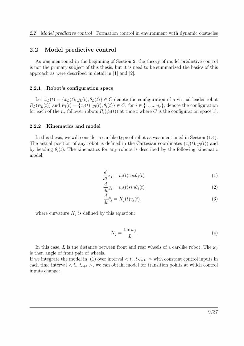
In this thesis, we will consider a car-like type of robot as was mentioned in Section (1.4).The actual position of any robot is defined in the Cartesian coordinates (xi(t), yi(t)) andby heading θi(t). The kinematics for any robots is described by the following kinematicmodel:

d

dtxj = vj(t)cosθj(t) (1)

d

dtyj = vj(t)sinθj(t) (2)

d

dtθj = Kj(t)vj(t), (3)

where curvature Kj is defined by this equation:

Kj =tanωj

L(4)

In this case, L is the distance between front and rear wheels of a car-like robot. The ωj

is then angle of front pair of wheels.If we integrate the model in (1) over interval < to, tN+M > with constant control inputs ineach time interval < tk, tk+1 >, we can obtain model for transition points at which controlinputs change:

9/37

2.2 Model predictive control Formation control in environment with dynamic obstacles

xj(k + 1) =

xj(k) + 1

Kj(k+1)[sinθj(k) +Kj(k + 1)vj(k + 1)∆t(k + 1))−

−sin(θj(k))], if Kj(k + 1) 6= 0;

xj(k) + vj(k + 1)cos(θj(k))∆t(k + 1), if Kj(k + 1) = 0

(5)

yj(k + 1) =

yj(k)− 1

Kj(k+1)[cosθj(k) +Kj(k + 1)vj(k + 1)∆t(k + 1))−

−sin(θj(k))], if Kj(k + 1) 6= 0;

yj(k) + vj(k + 1)sin(θj(k))∆t(k + 1), if Kj(k + 1) = 0

(6)

θ(k + 1) = θj(k) +Kj(k + 1)vj(k + 1)∆t(k + 1), (7)

where xj(k), yj(k) are the rectangular coordinates and θj(k) is the heading angle. Thismodel notation is useful for describing long trajectories exactly using a minimal amountof information. More detailed explanation can be found in [1].

2.2.3 Constraints

In MPC theory, the Cartesian coordinate system is used to determine the actual po-sition of any robot as was mentioned in the previous paragraph. But the main problemlies in determining the change of position over time, where the Cartesian system is inap-propriate because in the real experiments we must respect hardware propositions of therobot. The wheels of a car-like robot are limited by maximal and minimal curvature as wellas the engine has constrained power to actuate the wheels - this parameter we will takein consideration by defining velocity. These constraints can be expressed by the followinginequalities:

vmin,j ≤ vj(k) ≤ vmax,j (8)

|Kj(k)| ≤ Kmax,j, (9)

where vmax,j is the maximal forward velocity of the car-like robot, vmin,j is the maximalbackward velocity and Kmax,j is the maximal possible curvature.

2.2.4 Shape of a formation

The major problem during the computation of a new control point of any formationlies in the constrained curvatures as was explained in Section (2.2.3). When formation isturning, every robot has to execute a movement with different value of curvature. If inputcurvature to outer follower of a turning formation will be too small, limited range of innerfollowers will not be enough and collision becomes imminent.Another very important fact when driving formation of car-like robots is caused by the

10/37

2.3 Implemented models Formation control in environment with dynamic obstacles

inability to the change angle of heading of the robot on the spot. This problem was solvedby implementation of curvilinear coordinates instead of the Cartesian, which cannot beused. To convert the state of followers in curvilinear coordinates to the state of rectangularcoordinates, the following equation can be applied:

xi(t) = xL(tpi(t))− qi(tpi(t))sin(θL(tpi(t))) (10)

xi(t) = xL(tpi(t))− qi(tpi(t))sin(θL(tpi(t))) (11)

θi(t) = θL(tpi(t)) (12)

2.2.5 The cost function

The basic equation in the model predictive control theory is the minimization of thecost function JL(.) ,which is given by (13).

JL(ΩL) =N+M∑k=N+1

∆t(k) + α

n0∑j=1

(min

0,distj(ΩL,ΘObs)− rs,Ldistj(ΩL,ΘObs)− ra,L

)2

, (13)

where the first part of the formula expresses endeavor to reach a desired target as soonas possible and the second part accounts for expressing the influence of the environment.This influence has an impact on the final solution and we are able to control it’s cost byadjusting the α constant.

2.3 Implemented models

2.3.1 Rules extension for dynamic obstacles

The cost function in Section (13) is defined correctly for the leader only, but for thewhole formation we need to have an extended variant, which is composed of three com-ponents with their influence adjusted by constants α and β in (14). The first componentrepresents deviations of the desired position in the same way as in the previous equation.The second summation term is also the same as is mentioned in (13) and is responsiblefor detection of static or lately detected dynamic obstacles. The main difference is in thethird component with the β constant, which has been added to ensure avoiding collisionbetween other members of the formation by considering them as other dynamic obstaclesin the environment.

11/37


The main contribution of this thesis was the extension of model predictive control frame-work by dynamic obstacle avoidance. These rules were implemented into the second com-ponent of equation (14), where the position of obstacles dynamically changes with respectto time. It means that the solver can predict the next move of an obstacle in each iterationaccording to the input model.

Ji(Ωi) =N∑k=1

‖ (pd,i − pi(k)) ‖2 + α

n0∑j=1

(min

0,distj(Ωi,ΘObs(t))− rsdistj(Ωi,ΘObs(t))− ra

)2

+ β∑j∈nn

(min

0,di,j(Ωi,Ω

Oj )− rs,i

di,j(Ωi,ΩOj )− ra,i

)2

,

(14)

where rs is a circular detection boundary radius, ra is a circular avoidance boundaryradius for a single robot, Ω is a position of a robot and Θ is a position of an obstacle.

2.3.2 Linear model interpretation

In this subsection, we will introduce mathematical interpretation of the linear modelavoidance predictive method. The concept of obstacle movement is very similar to themodel of motion which was defined for robot leaders in Section 2.2. The main differencelies within input velocity, which remains constant during the whole computation. In thecase of linear model, we do not take curvature K in consideration. Actual position of virtualdynamic obstacle is defined by summation of partial changes over time by equations shownin (15). Initial position of dynamic obstacle is given by coordinates (xlm0 , ylm0 , θlm0), wherethe θlm0 remains constant. Actual position of a virtual marauder is given by (xlm(k), ylm(k)),where k is the local transition point.

xlm(kn+1) = xlm0 +n∑

k=1

∆xlm(kn) (15)

ylm(kn+1) = ylm0 +n∑

k=1

∆ylm(kn). (16)

where the actual Euclidean coordinates of position of robot marauder (dynamic obstacle)moving with straight heading and constant velocity is defined by the following equations:

∆xlm(k) = vlm sin(θlm)∆t (17)

∆ylm(k) = vlm sin(θlm)∆t (18)

θlm(k) = θlm0 , (19)

12/37


2.3.3 Quadratic model interpretation

The same concept as was described in Section 2.3.2 we can use in the case of interpre-tation of quadratic model but the input curvature Kqm must be taken in account. Actualstate of virtual dynamic obstacle with initialization coordinates (xqm0 , yqm0 , θqm0) is definedby the following equations:

xqm(kn+1) = xqm0 +n∑

k=1

∆xqm(kn) (20)

yqm(kn+1) = yqm0 +n∑

k=1

∆yqm(kn) (21)

θqm(kn+1) = θqm0 +n∑

k=1

∆θqm(kn), (22)

where the Euclidean coordinates of position of robot marauder (dynamic obstacle) mov-ing with straight heading and constant velocity is defined by the following equations:

∆xqm(k) =sin(θqm) +Kqmvqm∆t− sin(θqm)

Kqm

(23)

∆yqm(k) = −cos(θqm) +Kqmvqm∆t− sin(θqm)

Kqm

(24)

∆θqm(k) = Kqmvqm∆t, (25)

2.3.4 Implementation details

Inside the fitness function (14), the measure of an actual distance between marauder androbot leader is being executed in each iteration of a solver through the Euclidean metric,which is shown in Equation (26):

dist(ΩL,ΘMau) =

√√√√ 3∑n=1

(ΩLi−ΘMaui

), (26)

where n represents a system of coordinates (x, y, z) of a robot, ΩL defines an actualposition of leader and ΘMau is the position of a virtual marauder. A brief approximationof extended algorithm of model predictive control approach is shown in the Scenario 1:

13/37


→ description getVisibilityGraph;– Calling of visibility graph algorithm, which is responsible for creatinginitializing control inputs from the actual state of the world.→ description callSolver;– CallSolver is the core function of the whole algorithm, which on thebasis of control inputs, constraints and the final value of fitness functionevaluates the quality of solution. Also, this function can iteratively mea-sure the Euclidean distance of marauder and the rest of the formationas was described in equation ( 26).Algorithm;world = loadMap();control = getVisibilityGraph(world);leader→ init;followers→ init;marauder→ init;while dist2goal > 0 do

callSolver(state, end,N, control, constants);leader→ move(solution→ velocity, solution→ curvature, solution→ time);insertState(state, leaderPath);for i = 0; i < followers; i+ 1 do

formationi → callSolver(state, end,N, control, constants);insertState(state, followerPathi);

marauder→ move(predictiveModel);// on the real robotic platform (SyRoTek), here would be a feedback

controller, which would be taken in account an actual position of a

marauder;updateWorld(world);control = getVisibilityGraph(world);

Robot reached goal position;Scenario 1: The algorithm for trajectory planning using MPC approach with new rulesfor avoiding dynamic obstacles implemented.

14/37

2.4 Complicated maneuvers Formation control in environment with dynamic obstacles

Figure 5: The demonstration of measuring Euclidean distance between marauder andleader.

2.4 Complicated maneuvers

The implemented method of avoiding dynamic obstacles works on a predictive base, butsituations in which formation gets stuck can appear. This can be caused by incorrectlytuned predictive model or inaccurate movement of the real robot as a result of bad hard-ware propositions.

In this case, solution is valid in the sense of the input model, but the detected position8

of the dynamic obstacle does not correspond. This sets out the problem where dynamicobstacle is moving while the robot leader is executing a new trajectory so the found solu-tion is no longer acceptable and it has to be resolved according to new data. The qualityof solving this situation can be enhanced by model where the robot is continuously re-versing along the previous trajectory until it is in safe predefined minimal distance fromthe obstacle. Boundary for this precaution can be set by the constant that is defining theminimal safe distance to the obstacle. The robot then must repeat the process in a loopuntil the final solution is feasible. This algorithm can guarantee that the future solutionwill be feasible (assuming the obstacle remains at constant velocity and direction).

This process and final correctness of solution may be very sensitive to tuning up theconstants such as sensor sensitivity or distance that is considered as critical in the sense ofhardware and physical robot propositions. If the critical distance is tuned up badly, newsolution may not be feasible or even solvable. A flowchart of the precaution algorithm canbe found in Figure (6).

8From the distance sensor or global camera positioning system.

15/37

2.4 Complicated maneuvers Formation control in environment with dynamic obstacles

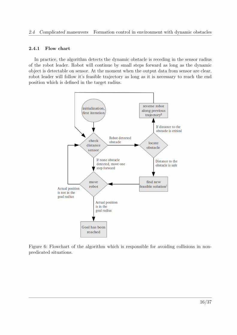
2.4.1 Flow chart

In practice, the algorithm detects the dynamic obstacle is receding in the sensor radiusof the robot leader. Robot will continue by small steps forward as long as the dynamicobject is detectable on sensor. At the moment when the output data from sensor are clear,robot leader will follow it’s feasible trajectory as long as it is necessary to reach the endposition which is defined in the target radius.

Figure 6: Flowchart of the algorithm which is responsible for avoiding collisions in non-predicated situations.

16/37


3 Simulations and results

The final results of this project are summarized in this chapter which consists of detailedreport of the experimental mission simulation executed by formation with car-like robotleader using predictive control algorithm for avoiding the dynamic obstacles.

3.1 Computer simulations

Following types of obstacle model movement ( 3.1.1 and 3.1.2) were implemented intothe model-predictive control framework, which is being developed at the Department ofCybernetics, CTU in Prague. As was mentioned in the Section (1.3), two ways of modelprediction were integrated. Results of experiments of both implemented models can befound in Section (3.3). In the simulations, two models of dynamic obstacles were testedaccording to following parameters:

• Linear model - constant velocity, curvature k = 0

• Quadratic model - constant velocity, curvature k > 0

All simulations and graphics in this section are generated in Gnuplot9.

3.1.1 Linear model

In this subsection, we are presenting an example of solved solution of solver with ex-tended rules of predictive control in the environment with dynamic obstacle. Followingfigures demonstrates numeric results for the concrete conditions with respect to the actualtime.

In the Figure 7 we can observe the beginning of the simulated mission, where the threeblue vehicles represent robotic formation, that are supposed to achieve target ring byfeasible trajectory. Red vehicle represents marauder (or broken) robot, that is movingstraight down through the optimal trajectory, which is marked by full black line. Thesecond image in the Figure 7 demonstrated critical part of a solution, where the drivenformation slowed down10 and turned to the left to avoid collision with the red car.

The second Figure 7 demonstrates the final part of the solution, where the red car isreceding and the formation is starting to balance trajectory to be optimal.

9Command-line driven graphic utility for Linux.10More static-time control points on a shorter distance

17/37

3.1 Computer simulations Formation control in environment with dynamic obstacles

Figure 7: Computer demonstration of a feasible solution solved by linear model of extendedrules of model predictive control.

18/37

3.1 Computer simulations Formation control in environment with dynamic obstacles

Figure 8: Computer demonstration of a feasible solution solved by quadratic model ofextended rules of model predictive control.

19/37

3.2 Quality of solution Formation control in environment with dynamic obstacles

3.1.2 Quadratic model

Example of movement of the formation using the algorithm with quadratic model of theobstacle employed for obstacle avoidance is presented in the figure 8. This time, red car isfollowing a circular path.

Quadratic model is characterized by constant velocity and curvature. Resulting move-ment of this setting can be seen in the following figures, where the red car is moving on acircle trajectory. New rules for model predictive control should provide a safe and feasiblesolution in sense of predictive avoiding as is demonstrated in the picture by curved trajec-tory of a blue robotic formation in the figure 8. Higher density of control points indicatesan effort to slow down before turning and to increase a distance between the car-like robotformation and the the red robot.

3.2 Quality of solution

The quality of the final solution can be compared among two implemented models by twodifferent criteria: final times which will show how quickly the formation can achieve targetregion and the minimal distance to collision from formation that is critical for feasibility ofthe final solution. In dynamic environment, bad tuned predictive model (or none model)can easily get into collision state with a moving obstacle. In the Figure 9, the comparisonof final trajectories of two solvers with different predictive model implemented for the sameinitialization conditions can be seen.

Figure 9: Comparison between linear and quadratic solver for the same initialization con-ditions.

This computer simulation (as is shown in the Figure 9 was executed for dynamic obstacle(robot marauder) that is moving according to the quadratic model. In case of the employedlinear model, robot formation does not account for curvature of a robot and after each

20/37

3.2 Quality of solution Formation control in environment with dynamic obstacles

iteration solver considers the heading of marauder as static. This can cause the situationas the one shown in the Figure 10, where the formation is in a direct collision with robotmarauder while solver with an accurate quadratic model implemented found a feasibletrajectory. Actual position of robot marauder (as is shown in 9) show that the solver withlinear predictive model implemented ended in shorter time than with quadratic predictionbut solved infeasible trajectory 10.

Figure 10: Demonstration of collision state of a badly tuned predictive model.

21/37

3.3 Results and graphs Formation control in environment with dynamic obstacles

3.3 Results and graphs

To verify implementation of new rules of model predictive control for driving formationin environment with dynamic obstacles, several computer simulations were executed, thatwill compare non-predictive rules of MPC with new extensions to predicate non-staticbarriers, as was described in Section 2.3.1.

These two models will be compared in several situations by following criteria:

• the minimal distance from the formation to collision state with the obstacle

• the final time of the solved trajectory

Both test will be playing a crucial role in the resulting quality of new implemented rulesfor driving robotic formations. Tests in 2.3.1 are divided into two independent parts withdifferent initial conditions. The first run of experiments was executed with linear model ofdynamic obstacle movement, while the second one was set to simulate quadratic model.The comparison was made by the following configuration:

Simulations

Linearobstacle

Quadraticobstacle

Minimal distanceto collision

Final time

Minimal distanceto collision

Final time

Linear modelStatic model

Linear modelStatic model

Quadratic model

For objectivity of the final numbers, in sum 2300 experiments were executed. All resultswere entered into a bar graph. In each simulation, randomly generated start position offormation was chosen.

3.3.1 Static vs. linear model

The first executed simulations demonstrate a comparison between static and linearmodel prediction of dynamic obstacle movement. In the Figure 11 we can see an averagetime to achieve final position of both model comparison. According to the figure, in thisseries of simulations, implementation of linear predictive model improved solution andshortened the final time for which the formation traveled on solved trajectory.

22/37


19.21Static19.02Linear

18.2 18.45 18.7 18.95 19.2time

Figure 11: Graphic comparison of static and linear model for linear movement of thedynamic obstacle (in sense of final time).

On the contrary, difference between measuring of the minimal distance to collision ofboth models are non-significant in this case. Figure 12 demonstrates that even well tunedmodel can not necessarily improve the final solution but also does not make it worse.


0 0.25 0.5 0.75 1 1.25distance

Figure 12: Graphic comparison of static and linear model for linear movement of thedynamic obstacle (in sense of minimal distance to collision).

3.3.2 All models comparison

Much more illustrative is comparison of all models for quadratic movement of the dy-namic obstacle. As we mentioned in Section (3.3.1), well tuned model should not makethe final solution worse then solver without any model (static). But if we use incorrectlytuned model, results can easily become worse or even strongly inappropriate (because ofinfeasible trajectory). In this series of simulation, we tested dynamic solver in situationwith dynamic obstacle, which is following a circle trajectory (constant velocity, k > 0),for both implemented predictive solver variants. In this case, the linear model behaves asbadly tuned quadratic model (zero curvature), which results in a much worse solutionsthen the solver without any model. This find sets out a conditions, where it is necessaryto use as good model as possible to achieve the best resulting trajectory.

23/37



18.35Quadratic

18.2 18.45 18.7 18.95 19.2time

Figure 13: Graphic comparison of all models for quadratic movement of the dynamic ob-stacle (in sense of final time).

Measuring of minimal distance from formation to collision with the dynamic obstaclealso brought an evidence that well tuned model improves the final solution while bad model(linear) can make the final solution make worse. In the Figure (14), solution by quadraticpredictive model showed significant improvement.


1.32Quadratic

0 0.25 0.5 0.75 1 1.25distance

Figure 14: Graphic comparison of all models for quadratic movement of the dynamic ob-stacle (in sense of minimal distance to collision).

24/37


4 Experiments with SyRoTek

To verify all new implemented rules of model-predictive control framework, the Sy-RoTek11 system was chosen as an appropriate real simulator.

Figure 15: One of twelve robots, that are forming an active part of a SyRoTek roboticsystem.

4.1 About SyRoTek

The SyRoTek system is a result of a project of the Czech Technical University in Prague,that allows students and scientists to develop their own algorithms on a multi-robot plat-form in a dynamic environment. System enables users to remotely control the whole plat-form without any external human intervention, because the maintenance is supposed to befully autonomous.

Communication interface between users and robots is provided by the Player Stage,where Player is designed to provide all necessary IP communication between robots, serverand users. Stage is an optional part of the software and enables to test and simulatealgorithms before uploading to the real system.

Whole system consists of a twelve autonomous robots equipped with several sensors tomerge distance, scan surface and detection of an actual orientation of a robot. In practice,most of all robots are fitted up with eight IR range sensors (five on the chassis and three in

11System for robotic e-learning

25/37

4.2 Computer simulation Formation control in environment with dynamic obstacles

the front), six sonars(three on the chassis and three in the front), compass, accelerometer,two floor sensors and laser range finder. In the near future, all robots will also be equippedwith cameras. Actual position of any robot in the arena can be detected through the onboard odometry sensors or by the global camera positioning system, that is much moreprecise for long-time measuring.

Implementation of all algorithms is realizing in C++ programming language with anappropriate libraries included. Source codes are then compiled and executed by Player onthe SyRoTek server. More information in detail can be found in [9].

Figure 16: Communication scheme of the SyRoTek system.

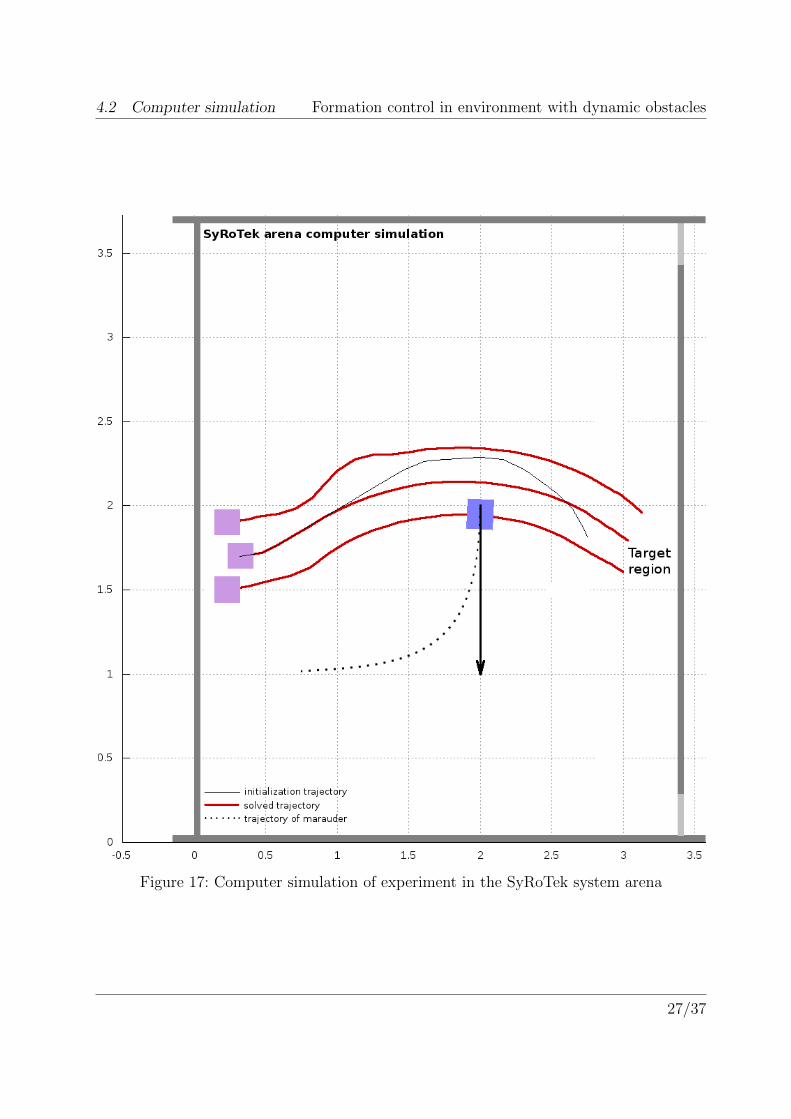
4.2 Computer simulation

Before executing the real experiment on the SyRoTek system, all initializing condi-tions and functionality of the solver with new rules implemented were tested and analyzedthrough the virtual computer simulation as it‘s showed in Figure (17). As dynamic obstacle,one of the SyRoTek robots was chosen to move according to quadratic model. Solver wastuned with very accurate input parameters for the best possible solution. Robot hardwarepropositions such as dimensions or velocity limits were also taken into account. As initial-ization trajectory (tiny black line in the Figure (17)), visibility graph with Dijkstra pathstate search algorithm was chosen. To ensure the most feasible input trajectory, visibilitygraph is generated dynamically in each iteration of computation of MPC solver.

26/37

4.2 Computer simulation Formation control in environment with dynamic obstacles

Figure 17: Computer simulation of experiment in the SyRoTek system arena

27/37

4.3 Experiments Formation control in environment with dynamic obstacles

4.3 Experiments

4.3.1 Initialization conditions

In this thesis, practical examples on a real robotic system of the new rules of modelpredictive control theory, were executed. For purposes of the experiments, static obstaclesin the arena were removed and localization system was properly modified. Tested formationconsisted of three robots - one robot leader and two followers. As a dynamic obstacle,another robot was chosen to move across the optimal trajectory of the formation in whichway the solver was forced to change the shape of path and ensure to be feasible for allmembers of the formation.

Experimental robotic mission was set up to achieve target region in cleared and emptyrobot arena. Without intervention of dynamic obstacle, an optimal trajectory leads straightfrom the start position. More complicated scenario could not be chosen, because of thelimited space in the arena.

4.3.2 Implementation details

As was mentioned in Section 4.1, all algorithms are implemented using C++ language.The source is structured into two main sections. The first part provides communicationwith Player to drive robots, while the second part counts the trajectory (solver of modelpredictive control) on the base of input data from sensors. For each robot in the arena,individual thread was implemented. All threads must be synchronized to ensure, that allrobots will be following the formation.

Final experiment was divided to offline and online computation. The main reason forthis separation is significant computation time of new control point of the MPC solver. Inpractice, after each step, all robots had to stop and wait for solver to finish all calculations.Because of this deceleration, an offline version of experiment was executed to demonstratefluent movement of the formation. To prevent anomaly hardware problems such as slippingwheels, an appropriate feedback controller was programmed. Both runs are documentedand attached as video record on CD for this thesis.

4.3.3 Mission

During both experiments, robots successfully followed a trajectory computed by thesolver. Noticeable anomalies caused by hardware were regulated through implementedfeedback controller. In the figures 18 and 19 recorded situations can be seen during theexperiments with graphical demonstration of executed trajectory that was calculated bythe solver of model predictive control.

28/37

4.3 Experiments Formation control in environment with dynamic obstacles

Figure 18: Camera record of SyRoTek system during the experiment.

Figure 19: Camera record of SyRoTek system during the experiment.

29/37

4.4 Experiences with system Formation control in environment with dynamic obstacles

4.4 Experiences with system

Although the SyRoTek system is almost at the final state of development, there is stilla lot of space for further improvements. In this thesis, work with real robotic system andimplementation of model predictive control algorithms into the SyRoTek system were oneof the most important issues in this project. Based on this experiences, several recommen-dations will be brought to help with further improvements of the system.

4.4.1 Recommendations

At the beginning of this bachelor project, working with the SyRoTek system was verydifficult and impractical. Problems started with official SyRoTek user manual which indetail described only special plugin for NetBeans IDE. But this plugin worked properlyonly on the specialized SyRoTek linux distribution, which was very slow and not suitablefor working with larger project. The only usable form of controlling and programmingthe system was through the linux terminal. Unfortunately, this way of using SyRoTekwould deserve much more complex documentation, because the only information aboutusing Player platform was located on the official website with a lot of redundant data(redundant for system users, not developers).

Next issue which should be mentioned was programming the system. Like documenta-tion, SyRoTek system would deserve more examples with multirobotic use. Services suchas integrated dynamic obstacles, camera access, manual robot driving or using syrcontrol12

were described nowhere. But this lack of information was apparently caused by the factthat this thesis was the first of its kind to work with the SyRoTek system.

The SyRoTek system is designed for 24 hours remote access and should provide anautonomous service, reservations management, docking robots and choosing an appropriaterobots for the individual reservation. But there are also issues that system cannot solveproperly. One of them is cleaning dust from the surface of the arena, that may cause slippingwheels of the robots. To solve this problem, a cleaning robot should by constructed. Butthe problem with sliding wheels is not only caused by dust. Next problem lies within themechanical system for ejecting integrated dynamic obstacles. The system sometimes slidesthe obstacle lower then the surface of the arena, where a robot can easily get stuck.

Another problem that occurred during the work with the SyRoTek was loosing local-ization of robots influenced by imperfect shielding of the arena from sunrays and otherexternal influences.

Due to the debugging of the whole system, the programming was accompanied by a lotof system failures, but they were usually very quickly solved by the service engineer Mr.Chudoba, whom I would like to thank for the willingness.

12Application for autonomous planning of a robot to user defined position.

30/37

4.4 Experiences with system Formation control in environment with dynamic obstacles

4.4.2 Brief summary of recommendations

More structured and brief summary of all recommendations can be found in the followinglist:

• Brief and structured documentation to control SyRoTek system from the Linux ter-minal.

• Possibility to download all camera records without asking for root access.

• More C++ source examples of how to program SyRoTek.

• Cleaning robot for removing dust from the surface of arena.

• Better shielding to deflect sunrays from the arena.

31/37


5 Conclusion

The main aim of this thesis was an integration, simulation and final verification of theextension of the model predictive control focused algorithms to avoid obstacles in dynamicenvironment. For purposes of this thesis, a working framework that is developed by theDepartment of Cybernetics CTU in Prague was provided.

All integrated algorithms were tested and simulated and results can be found in Ap-pendix of this thesis. Summarized results were discussed in Section (3). All results showedthat new extended rules of MPC work properly according to theory.

Verifying of new implemented rules of model predictive control theory on the real roboticsystem brought several interesting findings. One of them was the execution of two individualexperiments on the SyRoTek system, where online and offline computation had to be sep-arated and executed individually. The main reason of this arrangement was an insufficientcomputing power of the SyRoTek system. Comparison of these experiments demonstratesan advantage of online computation, where establishment of feedback controller had sig-nificant influence to final solution and the shape of formation stayed unchanged duringexecuting the whole trajectory.

For me, the experience with the SyRoTek robotic system was inspirational and providesvaluable experiences with the real robotic platform. For this occasion, a brief list of rec-ommendations for the future development of SyRoTek was written and can be found inSection (4.4.1). I hope this thesis will bring benefits and help for members of the SyRoTekproject in sense of future improvements and development of the whole platform.

5.1 Future of the project

As was mentioned in the motivation in the beginning of this thesis in Section (1.1.2)about possible applications, all simulations and experiments presented in this thesis areapplicable to practical use in the real world. The demonstration using the SyRoTek systemprovided a significant proof that with more computing power, driving the nonholonomicrobotic formations can be realized through the model-predictive control approach withimplemented rules for avoiding dynamic obstacles.

32/37

6 Appendix A

6.1 Tables of results

Table 1: Comparison of final times of all implemented models

Nr. no model linear quadratic1 19,5 19 20,52 19 19,5 18,53 18,5 20 17,54 19 19 205 18,5 19 186 18,5 21 217 18,5 19 18,58 18,5 20 189 20 19 2010 19 19 17,511 18,5 20 18,512 20 18,5 1813 20 20 1814 20 19,5 1815 20 20 1816 19 19,5 1817 18,5 19 2018 20 19 1919 19 19 18,520 19 19,5 1921 18,5 19 22,522 19 19,5 18,523 18,5 19 18,524 18,5 20 1925 19,5 22 18,5.. .. .. ..230 17,5 18,5 18average 18,69 18,97 18,35

6.1 Tables of results Formation control in environment with dynamic obstacles

Table 2: Comparison of minimal distances to collision of all models

Nr. no model linear quadratic1 0,53 1,05 0,282 1,09 0,47 1,053 1,33 0,74 1,774 0,98 1,02 0,665 1,10 1,07 1,686 1,10 0,68 1,037 1,09 1,02 1,378 1,13 0,26 1,469 0,41 1,05 0,6410 0,99 1,04 1,8211 1,09 0,25 1,0312 0,43 1,12 1,5013 0,73 0,69 1,5214 0,44 0,45 1,4215 0,37 0,72 1,4916 1,00 0,70 1,7517 1,10 1,06 0,4418 0,43 1,01 1,0319 1,06 1,03 1,3220 1,05 0,41 0,9821 1,11 1,04 0,3322 1,05 0,43 1,0823 1,08 1,02 1,0524 1,09 0,26 0,9925 0,49 0,72 1,0926 1,07 0,44 1,4627 1,07 0,44 1,4128 1,01 1,06 1,1029 1,05 1,01 0,1930 1,09 1,09 1,5031 1,32 0,69 1,3932 1,07 0,70 1,8333 1,09 1,03 1,4634 0,82 1,12 1,0135 1,02 0,74 0,99.. .. .. ..230 1,75 1,10 1,40average 1,16 0,97 1,32

34/37

6.1 Tables of results Formation control in environment with dynamic obstacles

Table 3: Linear movement of dynamic obstacle, comparison of final time and minimaldistance to collision

Nr. static linear static linear1 20 19,5 0,53 0,572 19,5 19,5 0,53 0,523 19,5 19 0,56 0,554 19,5 19 0,52 0,525 19,5 19,5 0,53 0,456 19,5 19,5 0,55 0,557 19,5 18,5 0,54 0,558 18,5 19 0,59 0,569 18,5 19 0,55 0,5810 19,5 19,5 0,40 0,5611 19 19 0,55 0,5812 19,5 19 0,53 0,5613 19 19,5 0,53 0,5714 19,5 19 0,53 0,5415 18,5 19 0,52 0,5416 18,5 19,5 0,21 0,5517 18,5 19 0,55 0,6018 19,5 19 0,41 0,5419 18 19 0,49 0,6120 19 19 0,54 0,5721 20 21 0,73 0,5922 18,5 18,5 0,55 0,5223 18 19 0,55 0,6124 18 19,5 0,55 0,5325 19,5 19 0,61 0,6426 19,5 19,5 0,54 0,5727 18,5 20,5 0,39 0,5228 18,5 19 0,55 0,6029 19,5 19 0,50 0,5630 19 19,5 0,54 0,4931 19,5 19 0,39 0,6032 18,5 19,5 0,47 0,5833 19,5 19 0,49 0,5634 18 19 0,55 0,5735 19 19,5 0,49 0,55.. .. .. .. ..230 18 19 0,56 0,62average 19,21 19,02 0,57 0,56

35/37


7 Appendix B

CD Content

In table 4 are listed names of all root directories on CD

Directory name Descriptionbp bachelor thesis in pdf format.sources source codes for MPCsyrotek source codes for the SyRoTek systemtables tables of resultsvideo the SyRoTek experiment record

Table 4: CD Content

36/37

REFERENCES Formation control in environment with dynamic obstacles

References

[1] Saska M. Trajectory planning and optimal control for formations of autonomous robots.In Schriftenreihe Wurtzburger Forschungsberichte in Robotik und Telematik. Wurzburg:Universitat Wurzburg. ISSN 1868-7466, volume Band 3, 2010.

[2] Saska M., Mejıa S. J., Stipanovic M. D., and Schilling K. Control and Navigation of For-mations of Car-Like Robots on a Receding Horizon. In IEEE International Conferenceon Control Applications, 2009.

[3] Dunbar D. W. and Murray M. M. Distributed receding horizon control for multi-vehicleformation stabilization. In Automatica, pages 42(4):549–558, 2006.

[4] Dimarogonas D. V., Loizou S. G., Kyriakopoulos K. J., and Zavlanos M. M. A Feed-back Stabilization and Collision Avoidance Scheme for Multiple Independent Non-pointAgents. In Automatica, pages 42(2):229–243, 2006.

[5] Fierro R., Das K. A., Kumar V. R., and Ostrowski P. J. Hybrid Control of Formationsof Robots. In Proc. of IEEE Conference on Robotics and Automation,, 2001.

[6] Jaeger M. and Nebel B. Dynamic Decentralized Are Partitioning for CooperatingCleaning Robots. In Proc. of the IEEE Int. Conf. on Robotics and Automation (ICRA).

[7] Hardin T. C., Cui X., Ragade K. R., Graham H. J., and Elmaghraby S. A. A modifiedparticle swarm algorithm for robotic mapping of hazardous environments. In Proc. ofWorld Automation Congress, 2004.

[8] Yang S. X. and Luo C. A neural network approach to complete coverage path planning.In IEEE Transactions on Systems, Man, and Cybernetics, pages 34(1):718–724, 2004.

[9] Kulich M., Kosnar K., Chudoba J., Faigl J., and Preucil L. On a Mobile RoboticsE-learning System. In Proceedings of the Twentieth European Meeting on Cyberneticsand Systems Research. Vienna: Austrian Society for Cybernetics Studies. ISBN 978-3-85206-178-8, pages 597–602, 2010.

37/37

Formation control in environment with dynamic obstacles...

Documents

Transcript of Formation control in environment with dynamic obstacles...