Formalizing an SSA-based Compiler for Verified …stevez/vellvm/Zhao13.pdf · FORMALIZING AN...
136
FORMALIZING AN SSA-BASED COMPILER FOR VERIFIED ADVANCED PROGRAM TRANSFORMATIONS Jianzhou Zhao A DISSERTATION in Computer and Information Science Presented to the Faculties of the University of Pennsylvania in Partial Fulfillment of the Requirements for the Degree of Doctor of Philosophy 2013 Steve Zdancewic, Associate Professor of Computer and Information Science Supervisor of Dissertation Jianbo Shi, Associate Professor of Computer and Information Science Graduate Group Chairperson Dissertation Committee Andrew W. Appel, Professor, Princeton University Milo M. K. Martin, Associate Professor of Computer and Information Science Benjamin Pierce, Professor of Computer and Information Science Stephanie Weirich, Associate Professor of Computer and Information Science
Transcript of Formalizing an SSA-based Compiler for Verified …stevez/vellvm/Zhao13.pdf · FORMALIZING AN...
FORMALIZING AN SSA-BASED COMPILER FOR VERIFIED
ADVANCED PROGRAM TRANSFORMATIONS
Jianzhou Zhao
A DISSERTATION
in
Computer and Information Science
Presented to the Faculties of the University of Pennsylvania
in
Partial Fulfillment of the Requirements for the
Degree of Doctor of Philosophy
2013
Steve Zdancewic, Associate Professor of Computer and Information ScienceSupervisor of Dissertation
Jianbo Shi, Associate Professor of Computer and Information ScienceGraduate Group Chairperson
Dissertation Committee
Andrew W. Appel, Professor, Princeton University
Milo M. K. Martin, Associate Professor of Computer and Information Science
Benjamin Pierce, Professor of Computer and Information Science
Stephanie Weirich, Associate Professor of Computer and Information Science
Formalizing an SSA-based Compiler for Verified Advanced Program Transformations
COPYRIGHT
2013
Jianzhou Zhao

iii
ABSTRACT
FORMALIZING AN SSA-BASED COMPILER FOR VERIFIED ADVANCED PROGRAM
TRANSFORMATIONS
Jianzhou Zhao
Supervisor: Steve Zdancewic
Compilers are not always correct due to the complexity of language semantics and transformation algo-
rithms, the trade-offs between compilation speed and verifiability, etc. The bugs of compilers can undermine
the source-level verification efforts (such as type systems, static analysis, and formal proofs) and produce
target programs with different meaning from source programs. Researchers have used mechanized proof
tools to implement verified compilers that are guaranteed to preserve program semantics and proved to be
more robust than ad-hoc non-verified compilers.
The goal of the dissertation is to make a step towards verifying an industrial strength modern compiler—
LLVM, which has a typed, SSA-based, and general-purpose intermediate representation, therefore allowing
more advanced program transformations than existing approaches. The dissertation formally defines the
sequential semantics of the LLVM intermediate representation with its type system, SSA properties, memory
model, and operational semantics. To design and reason about program transformations in the LLVM IR,
we provide tools for interacting with the LLVM infrastructure and metatheory for SSA properties, memory
safety, dynamic semantics, and control-flow-graphs. Based on the tools and metatheory, the dissertation
implements verified and extractable applications for LLVM that include an interpreter for the LLVM IR, a
transformation for enforcing memory safety, translation validators for local optimizations, and verified SSA
construction transformation.
This dissertation shows that formal models of SSA-based compiler intermediate representations can
be used to verify low-level program transformations, thereby enabling the construction of high-assurance
compiler passes.
iv
Contents
1 Introduction 1
2 Background 4
2.1 Program Refinement . . . . . . . . . . . . . . . . . . . . . . . . . . . . . . . . . . . . . . 4
2.2 Static Single Assignment . . . . . . . . . . . . . . . . . . . . . . . . . . . . . . . . . . . . 6
2.3 LLVM . . . . . . . . . . . . . . . . . . . . . . . . . . . . . . . . . . . . . . . . . . . . . . 8
2.4 The Simple SSA Language—Vminus . . . . . . . . . . . . . . . . . . . . . . . . . . . . . 9
3 Mechanized Verification of Computing Dominators 11
3.1 The Specification of Computing Dominators . . . . . . . . . . . . . . . . . . . . . . . . . . 12
3.1.1 Dominance . . . . . . . . . . . . . . . . . . . . . . . . . . . . . . . . . . . . . . . 12
3.1.2 Specification . . . . . . . . . . . . . . . . . . . . . . . . . . . . . . . . . . . . . . 14
3.1.3 Instantiations . . . . . . . . . . . . . . . . . . . . . . . . . . . . . . . . . . . . . . 15
3.2 The Allen-Cocke Algorithm . . . . . . . . . . . . . . . . . . . . . . . . . . . . . . . . . . 16
3.2.1 DFS: PO-numbering . . . . . . . . . . . . . . . . . . . . . . . . . . . . . . . . . . 17
3.2.2 Kildall’s algorithm . . . . . . . . . . . . . . . . . . . . . . . . . . . . . . . . . . . 20
3.2.3 The AC algorithm . . . . . . . . . . . . . . . . . . . . . . . . . . . . . . . . . . . 22
3.3 Extension: the Cooper-Harvey-Kennedy Algorithm . . . . . . . . . . . . . . . . . . . . . . 23
3.3.1 Correctness . . . . . . . . . . . . . . . . . . . . . . . . . . . . . . . . . . . . . . . 24
3.4 Constructing Dominator Trees . . . . . . . . . . . . . . . . . . . . . . . . . . . . . . . . . 25
3.5 Dominance Frontier . . . . . . . . . . . . . . . . . . . . . . . . . . . . . . . . . . . . . . . 27
3.6 Performance Evaluation . . . . . . . . . . . . . . . . . . . . . . . . . . . . . . . . . . . . . 28
4 The Semantics of Vminus 30
v
4.1 Dynamic Semantics . . . . . . . . . . . . . . . . . . . . . . . . . . . . . . . . . . . . . . . 30
4.2 Dominance Analysis . . . . . . . . . . . . . . . . . . . . . . . . . . . . . . . . . . . . . . 32
4.3 Static Semantics . . . . . . . . . . . . . . . . . . . . . . . . . . . . . . . . . . . . . . . . . 33
5 Proof Techniques for SSA 35
5.1 Safety of Vminus . . . . . . . . . . . . . . . . . . . . . . . . . . . . . . . . . . . . . . . . 36
5.2 Generalizing Safety to Other SSA Invariants . . . . . . . . . . . . . . . . . . . . . . . . . . 37
5.3 The Correctness of SSA-based Transformations . . . . . . . . . . . . . . . . . . . . . . . . 38
6 The formalism of the LLVM IR 41
6.1 The Syntax . . . . . . . . . . . . . . . . . . . . . . . . . . . . . . . . . . . . . . . . . . . 41
6.2 The Static Semantics . . . . . . . . . . . . . . . . . . . . . . . . . . . . . . . . . . . . . . 46
6.3 A Memory Model for the LLVM IR . . . . . . . . . . . . . . . . . . . . . . . . . . . . . . 47
6.3.1 Rationale . . . . . . . . . . . . . . . . . . . . . . . . . . . . . . . . . . . . . . . . 47
6.3.2 LLVM memory commands . . . . . . . . . . . . . . . . . . . . . . . . . . . . . . . 48
6.3.3 The byte-oriented representation . . . . . . . . . . . . . . . . . . . . . . . . . . . . 49
6.3.4 The LLVM flattened values and memory accesses . . . . . . . . . . . . . . . . . . . 51
6.4 Operational Semantics . . . . . . . . . . . . . . . . . . . . . . . . . . . . . . . . . . . . . 51
6.4.1 Nondeterminism in the LLVM operational semantics . . . . . . . . . . . . . . . . . 52
6.4.2 Nondeterministic operational semantics of the SSA form . . . . . . . . . . . . . . . 55
6.4.3 Partiality, preservation, and progress . . . . . . . . . . . . . . . . . . . . . . . . . . 56
6.4.4 Deterministic refinements . . . . . . . . . . . . . . . . . . . . . . . . . . . . . . . 57
6.5 Extracting an Interpreter . . . . . . . . . . . . . . . . . . . . . . . . . . . . . . . . . . . . 59
7 Verified SoftBound 61
7.1 Formalizing SoftBound for the LLVM IR . . . . . . . . . . . . . . . . . . . . . . . . . . . 62
7.2 Extracted Verified Implementation of SoftBound . . . . . . . . . . . . . . . . . . . . . . . 67
8 Verified SSA Construction for LLVM 70
8.1 The mem2reg Optimization Pass . . . . . . . . . . . . . . . . . . . . . . . . . . . . . . . . 70
8.2 The vmem2reg Algorithm . . . . . . . . . . . . . . . . . . . . . . . . . . . . . . . . . . . . 77
8.3 Correctness of vmem2reg . . . . . . . . . . . . . . . . . . . . . . . . . . . . . . . . . . . . 80
vi
8.3.1 Preserving promotability . . . . . . . . . . . . . . . . . . . . . . . . . . . . . . . . 80
8.3.2 Preserving well-formedness . . . . . . . . . . . . . . . . . . . . . . . . . . . . . . 81
8.3.3 Program refinement . . . . . . . . . . . . . . . . . . . . . . . . . . . . . . . . . . . 83
8.3.4 The correctness of vmem2reg . . . . . . . . . . . . . . . . . . . . . . . . . . . . . 87
8.4 Extraction and Performance Evaluation . . . . . . . . . . . . . . . . . . . . . . . . . . . . 88
8.5 Optimized vmem2reg . . . . . . . . . . . . . . . . . . . . . . . . . . . . . . . . . . . . . . 89
8.5.1 O1 Level—Pipeline fusion . . . . . . . . . . . . . . . . . . . . . . . . . . . . . . . 90
8.5.2 O2 Level—Minimal φ-nodes Placement . . . . . . . . . . . . . . . . . . . . . . . . 93
9 The Coq Development 96
9.1 Definitions . . . . . . . . . . . . . . . . . . . . . . . . . . . . . . . . . . . . . . . . . . . . 96
9.2 Proofs . . . . . . . . . . . . . . . . . . . . . . . . . . . . . . . . . . . . . . . . . . . . . . 97
9.3 OCaml Bindings and Coq Extraction . . . . . . . . . . . . . . . . . . . . . . . . . . . . . . 98
10 Related Work 99
11 Conclusions and Future Work 102
Bibliography 105
Appendix A: The Correctness of vmem2reg-O1 113
Appendix B: The Correctness of vmem2reg-O2 122
vii
List of Figures
2.1 Simulation diagrams that imply program refinement. . . . . . . . . . . . . . . . . . . . . . . . 6
2.2 An SSA-based optimization. . . . . . . . . . . . . . . . . . . . . . . . . . . . . . . . . . . . . 8
2.3 The LLVM compiler infrastructure . . . . . . . . . . . . . . . . . . . . . . . . . . . . . . . . . 8
2.4 Syntax of Vminus . . . . . . . . . . . . . . . . . . . . . . . . . . . . . . . . . . . . . . . . . . 9
3.1 The specification of algorithms that find dominators. . . . . . . . . . . . . . . . . . . . . . . . 14
3.2 Algorithms of computing dominators . . . . . . . . . . . . . . . . . . . . . . . . . . . . . . . . 15
3.3 The postorder (left) and the DFS execution sequence (right). . . . . . . . . . . . . . . . . . . . 16
3.4 The DFS algorithm. . . . . . . . . . . . . . . . . . . . . . . . . . . . . . . . . . . . . . . . . . 17
3.5 Termination of the DFS algorithm. . . . . . . . . . . . . . . . . . . . . . . . . . . . . . . . . . 18
3.6 Inductive principle of the DFS algorithm. . . . . . . . . . . . . . . . . . . . . . . . . . . . . . 20
3.7 Kildall’s algorithm. . . . . . . . . . . . . . . . . . . . . . . . . . . . . . . . . . . . . . . . . . 21
3.8 The dominator trees (left) and the execution of CHK (right). . . . . . . . . . . . . . . . . . . . 24
3.9 The definition and well-formedness of dominator trees. . . . . . . . . . . . . . . . . . . . . . . 26
3.10 Analysis overhead over LLVM’s dominance analysis for our extracted analysis. . . . . . . . . . 28
4.1 Operational Semantics of Vminus (excerpt) . . . . . . . . . . . . . . . . . . . . . . . . . . . . 31
4.2 Static Semantics of Vminus (excerpt) . . . . . . . . . . . . . . . . . . . . . . . . . . . . . . . 33
6.1 Syntax for LLVM (1). . . . . . . . . . . . . . . . . . . . . . . . . . . . . . . . . . . . . . . . 42
6.2 Syntax for LLVM (2). . . . . . . . . . . . . . . . . . . . . . . . . . . . . . . . . . . . . . . . 43
6.3 An example use of LLVM’s memory operations. . . . . . . . . . . . . . . . . . . . . . . . . . . 44
6.4 Vellvm’s byte-oriented memory model. . . . . . . . . . . . . . . . . . . . . . . . . . . . . . . 49
6.5 Relations between different operational semantics, which are justified by proofs in Vellvm. . . . 52
viii
6.6 LLVMND: Small-step, nondeterministic semantics of the LLVM IR (selected rules). . . . . . . . 53
7.1 SBspec: The specification semantics for SoftBound. Differences from the LLVMND rules are
highlighted. . . . . . . . . . . . . . . . . . . . . . . . . . . . . . . . . . . . . . . . . . . . . . 63
7.2 Simulation relations of the SoftBound pass . . . . . . . . . . . . . . . . . . . . . . . . . . . . . 66
7.3 Execution time overhead of the extracted and the C++ version of SoftBound . . . . . . . . . . . 68
8.1 The tool chain of the LLVM compiler . . . . . . . . . . . . . . . . . . . . . . . . . . . . . . . 71
8.2 Normalized execution time improvement of the LLVM’s mem2reg, LLVM’s O1, and LLVM’s
O3 optimizations over the LLVM baseline with optimizations disabled. For comparison, GCC-
O3’s speedup over the same baseline is also shown. . . . . . . . . . . . . . . . . . . . . . . . . 72
8.3 The algorithm of mem2reg . . . . . . . . . . . . . . . . . . . . . . . . . . . . . . . . . . . . . 73
8.4 The SSA construction by the mem2reg pass . . . . . . . . . . . . . . . . . . . . . . . . . . . . 74
8.5 The SSA construction by the vmem2reg pass . . . . . . . . . . . . . . . . . . . . . . . . . . . 76
8.6 Basic structure of vmem2reg_fn . . . . . . . . . . . . . . . . . . . . . . . . . . . . . . . . . . 77
8.7 The algorithm of vmem2reg . . . . . . . . . . . . . . . . . . . . . . . . . . . . . . . . . . . . 79
8.8 The simulation relation for the correctness of φ-node placement . . . . . . . . . . . . . . . . . 84
8.9 The simulation relation for DSE and DAE . . . . . . . . . . . . . . . . . . . . . . . . . . . . . . 86
8.10 Execution speedup over LLVM -O0 for both the extracted vmem2reg and the original mem2reg. 88
8.11 Compilation overhead over LLVM’s original mem2reg. . . . . . . . . . . . . . . . . . . . . . . 89
8.12 Basic structure of vmem2reg-O1 . . . . . . . . . . . . . . . . . . . . . . . . . . . . . . . . . . 90
8.13 eliminate stld of vmem2reg-O1 . . . . . . . . . . . . . . . . . . . . . . . . . . . . . . . . . . 91
8.14 The operations for elimination actions . . . . . . . . . . . . . . . . . . . . . . . . . . . . . . . 92
8.15 Basic structure of vmem2reg-O2 . . . . . . . . . . . . . . . . . . . . . . . . . . . . . . . . . . 94
8.16 eliminate stld of vmem2reg-O2 . . . . . . . . . . . . . . . . . . . . . . . . . . . . . . . . . . 94
11.1 The effectiveness of GVN . . . . . . . . . . . . . . . . . . . . . . . . . . . . . . . . . . . . . 103
11.2 The effectiveness of Alias Analysis . . . . . . . . . . . . . . . . . . . . . . . . . . . . . . . . . 103
1 The algorithm of inserting φ-nodes . . . . . . . . . . . . . . . . . . . . . . . . . . . . . . . . . 122
ix
List of Tables
3.1 Worst-case behavior. . . . . . . . . . . . . . . . . . . . . . . . . . . . . . . . . . . . . . . . . 29
9.1 Size of the development (approx. lines of code) . . . . . . . . . . . . . . . . . . . . . . . . . . 97
List of Abbreviations
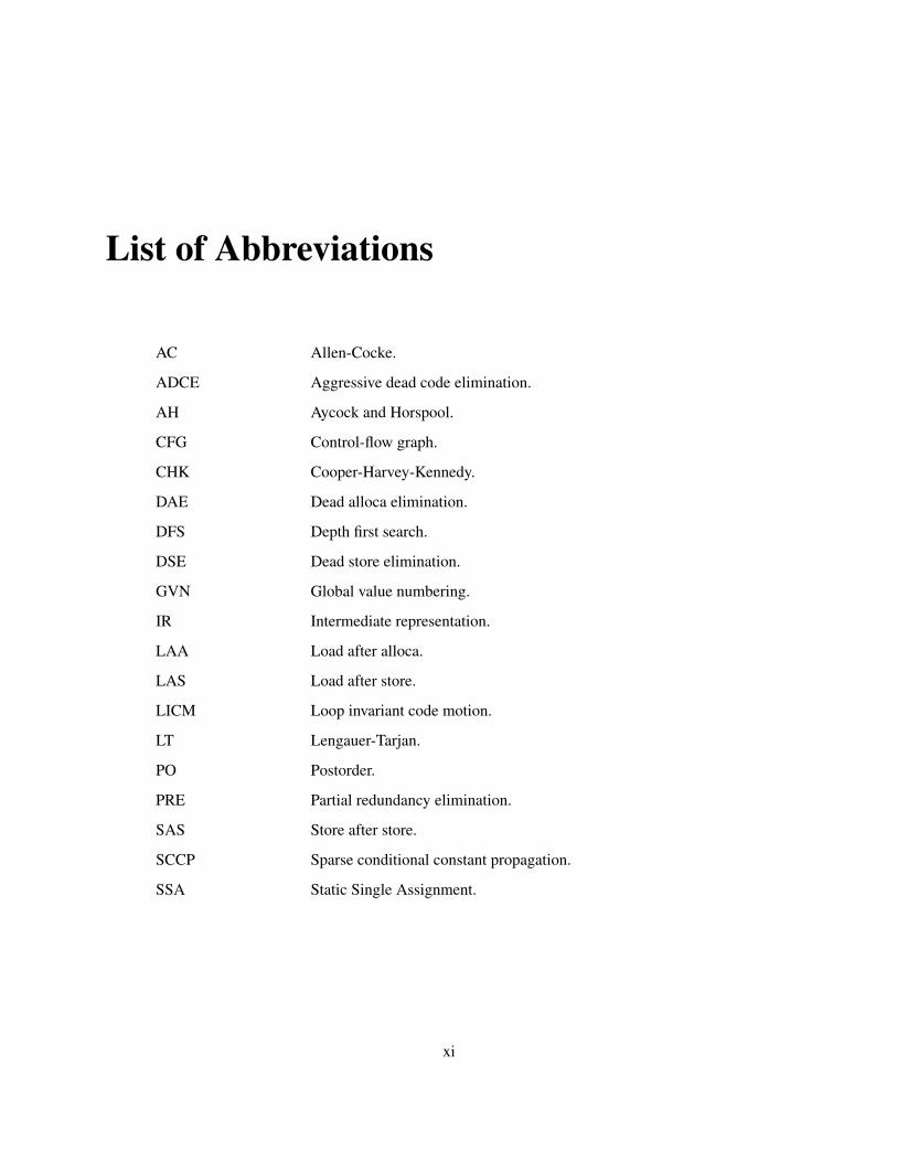
AC Allen-Cocke.
ADCE Aggressive dead code elimination.
AH Aycock and Horspool.
CFG Control-flow graph.
CHK Cooper-Harvey-Kennedy.
DAE Dead alloca elimination.
DFS Depth first search.
DSE Dead store elimination.
GVN Global value numbering.
IR Intermediate representation.
LAA Load after alloca.
LAS Load after store.
LICM Loop invariant code motion.
LT Lengauer-Tarjan.
PO Postorder.
PRE Partial redundancy elimination.
SAS Store after store.
SCCP Sparse conditional constant propagation.
SSA Static Single Assignment.
xi
Chapter 1
Introduction
Compiler bugs can manifest as crashes during compilation or even result in the silent generation of incorrect
program binaries. Such mis-compilations can introduce subtle errors that are difficult to diagnose and gen-
erally puzzling to the software developers. A recent study [73] used random test-case generation to expose
serious bugs in mainstream compilers including GCC [2], LLVM [38], and commercial tools. Whereas few
bugs were found in the front end of the compiler, various optimization phases of the compiler that aim to
make the generated program faster was a prominent source of bugs.
Improving the correctness of compilers is a worthy goal. Large-scale source-code verification efforts
(such as the seL4 OS kernel [36] and Airbus’s verification of fly-by-wire software [61]), program invariants
checked by sophisticated type systems (such as Haskell and OCaml), and sound program synthesis (for
example, Matlab/Simulink parallelizes high-level languages into C to achieve high performance [3]) can be
undermined by an incorrect compiler. The need for correct compilers is amplified when compilers are parts
of the trusted computing base in modern computer systems that include mission-critical financial servers,
life-critical pacemaker firmware, and operating systems.
Verified Compilers are tackling the problem of compiler bugs by giving a rigorous proof that a compiler
preserves the behavior of programs. The CompCert project [42, 68, 69, 70] first implemented a realistic and
mechanically verified compiler that is programmed and mechanically verified in the Coq proof assistant [25]
and generates compact and efficient assembly code for a large fragment of the C language. The aforemen-
tioned study [73] supports the effectiveness of this approach. Whereas the study uncovered many bugs in
other compilers, the only bugs found in CompCert were in those parts of the compiler not formally verified:
1
“The apparent unbreakability of CompCert supports a strong argument that developing compileroptimizations within a proof framework, where safety checks are explicit and machine-checked,has tangible benefits for compiler users.”
Despite CompCert’s groundbreaking compiler-verification efforts, there still remain many challenges in
applying its technology to industrial-strength compilers. In particular, the original CompCert development
and the bulk of the subsequent work—with the notable exception of CompCertSSA [14] (which is concurrent
with our work)—did not use a static single assignment (SSA) [28] intermediate representation (IR), as
Leroy [42] explains:
“Since the beginning of CompCert we have been considering using SSA-based intermediatelanguages, but were held off by two difficulties. First, the dynamic semantics for SSA is notobvious to formalize. Second, the SSA property is global to the code of a whole function andnot straightforward to exploit locally within proofs.”
In SSA, each variable is assigned statically only once and each variable definition must dominate all of
its uses in the control-flow graph. These SSA properties simplify or enable many compiler optimizations [49,
71] including: sparse conditional constant propagation (SCCP), aggressive dead code elimination (ADCE),
global value numbering (GVN), common subexpression elimination (CSE), global code motion, partial
redundancy elimination (PRE), inductive variable analysis (indvars) and etc. Consequently, open-source
and commercial compilers such as GCC [2], LLVM [38], Java HotSpot JIT [57], Soot framework [58], and
Intel CC [59] use SSA-based IRs.
Despite their importance, there are few mechanized formalizations of the correctness properties of SSA
transformations. This dissertation tackles this problem by developing formal semantics and proof techniques
suitable for mechanically verifying the correctness of SSA-based compilers. We do so in the context of our
Vellvm framework, which formalizes the operational semantics of programs expressed in LLVM’s SSA-
based IR [43] and provides Coq [25] infrastructure to facilitate mechanized proofs of properties about
transformations on the LLVM IR. Moreover, because the LLVM IR is expressive to represent arbitrary
program constructors, maintain properties from high-level programs, and hide details about target platforms,
we define Vellvm’s memory model to encode data along with high-level type information and to support
arbitrary bit-width integers, padding, and alignment issues.
The Vellvm infrastructure, along with Coq’s facility for extracting executable code from constructive
proofs, enables Vellvm users to manipulate LLVM IR code with high confidence in the results. For example,
2
using this framework, we can extract verified LLVM transformations that plug directly into the LLVM
compiler.
In summary, Thesis statement: Formal models of SSA-based compiler intermediate representations can be used to verifylow-level program transformations, thereby enabling the construction of high-assurance compiler passes.
Contributions The specific contributions of the dissertation include:
• The dissertation formally defines the sequential semantics of the industrial strength modern compiler
intermediate representation—the LLVM IR that includes its type system, SSA properties, memory
model, and operational semantics.
• To design and reason about program transformations in the IR, the dissertation designs tools for in-
teracting with the LLVM infrastructure, and metatheory for SSA properties, memory safety, dynamic
semantics, and control-flow-graphs.
• Based on the tools and metatheory, we implement verified and extractable applications for LLVM that
include the interpreter of the LLVM IR, a transformation for enforcing memory safety, translation
validators for local optimizations, and SSA construction.
The dissertation is based on our published work [75, 76, 77]. The rest of the dissertation is organized
as follows: Chapter 2 presents the background and preliminaries used in the dissertation. To streamline the
formalization of the SSA-based transformations, Chapter 2 also describes Vminus, a simpler subset of our
full LLVM formalization—Vellvm [75], but one that still captures the essence of SSA. Chapter 3 formalizes
one crucial component of SSA-based compilers—computing dominators [77]. Chapter 4 shows the dynamic
and static semantics of Vminus. Chapter 5 describes the proof techniques we have developed for formalizing
properties of SSA-style intermediate representations in the context of Vminus [76]. To demonstrate that our
proof techniques can be used for practical compiler optimizations, Chapter 6 shows the syntax of the full
LLVM IR—Vellvm. Then, Chapter 6 formalizes the semantics of Vellvm. Chapter 7 presents an application
of Vellvm—a verified program transformation that hardens C programs against spatial memory safety vio-
lations (e.g., buffer overflows, array indexing errors, and pointer arithmetic errors). Chapter 8 demonstrates
that our proof techniques developed in Chapter 5 can be used for practical compiler optimizations in Vellvm:
verifying the most performance-critical optimization pass in LLVM’s compilation strategy—the mem2reg
pass [76]. Chapter 9 summarizes our Coq development. Finally, Chapter 10 discusses the related work, and
Chapter 11 concludes.
3
Chapter 2
Background
This chapter presents the background and preliminaries used in the dissertation.
2.1 Program Refinement
In this dissertation, we prove the correctness of a compiler by showing that its output program P′ preserves
the semantics of its original program P: informally, P′ cannot do more than what P does, although P′ can
have fewer behaviors than P. With this correctness, a compiler ensures that the analysis and verification
results for source programs still hold after compilation.
Formally, we use program refinement to formalize semantic preservation. Following the CompCert
project [42], we define program refinement in terms of programs’ external behaviors (which include program
traces of input-output events, whether a program terminates, and the returned value if a program terminates):
a transformed program refines the original if the behaviors of the original program include all the behaviors
of the transformed program. We define the operational semantics using traces of a labeled transition system.
Events e : : = v = fid(vjj )
Finite traces t : : = ε | e, t
Finite or infinite traces T : : = ε | e,T (coinductive)
We denote one small-step of evaluation as config ` S t−→ S′: in program environment config, program state S
transitions to the state S′, recording events e of the transition in the trace t. An event e describes the inputs vj
and output v of an external function call named fid. config ` S t ∗−→S′ denotes the reflexive, transitive closure
4
of the small-step evaluation with a finite trace t. config ` S T−→ ∞ denotes a diverging evaluation starting
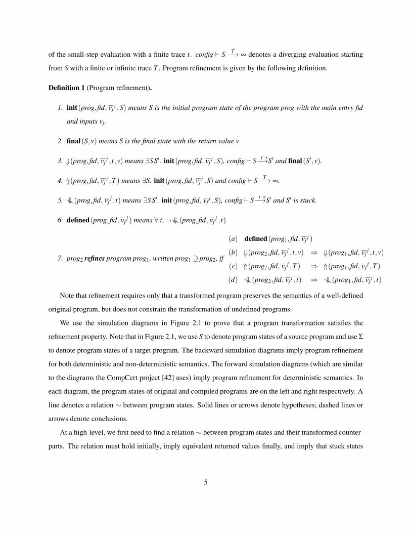
from S with a finite or infinite trace T . Program refinement is given by the following definition.
Definition 1 (Program refinement).
1. init(prog,fid, vjj ,S) means S is the initial program state of the program prog with the main entry fid
and inputs vj.
2. final(S,v) means S is the final state with the return value v.
3. ⇐(prog,fid, vjj , t,v) means ∃SS′. init(prog,fid, vj
j ,S), config ` S t ∗−→S′ and final(S′,v).
4. ⇒(prog,fid, vjj ,T ) means ∃S. init(prog,fid, vj
j ,S) and config ` S T−→ ∞.
5. 6⇐ (prog,fid, vjj , t) means ∃SS′. init(prog,fid, vj
j ,S), config ` S t ∗−→S′ and S′ is stuck.
6. defined(prog,fid, vjj ) means ∀ t, ¬ 6⇐ (prog,fid, vj
j , t)
7. prog2 refines program prog1, written prog1⊇ prog2, if
(a) defined(prog1,fid, vjj )
(b) ⇐(prog2,fid, vjj , t,v) ⇒ ⇐(prog1,fid, vj
j , t,v)
(c) ⇒(prog2,fid, vjj ,T ) ⇒ ⇒(prog1,fid, vj
j ,T )
(d) 6⇐ (prog2,fid, vjj , t) ⇒ 6⇐ (prog1,fid, vj
j , t)
Note that refinement requires only that a transformed program preserves the semantics of a well-defined
original program, but does not constrain the transformation of undefined programs.
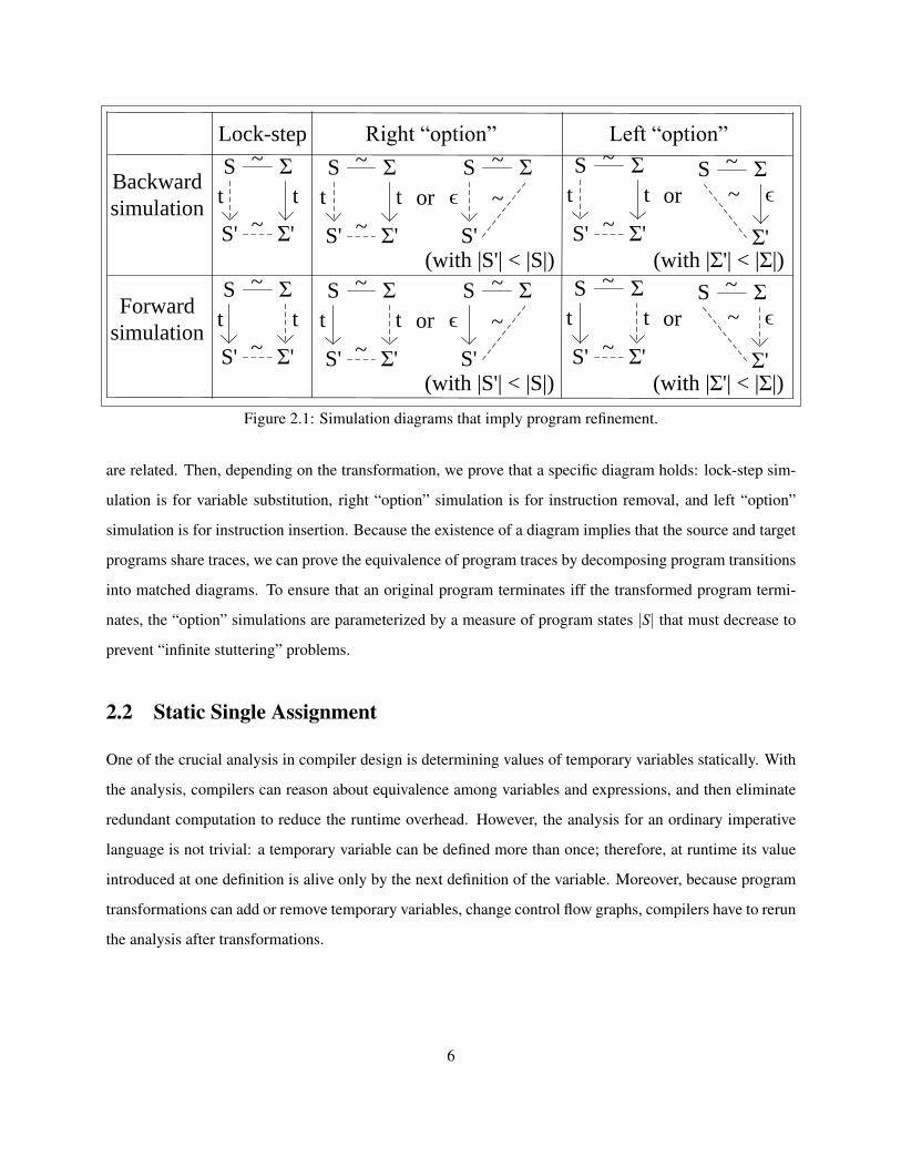
We use the simulation diagrams in Figure 2.1 to prove that a program transformation satisfies the
refinement property. Note that in Figure 2.1, we use S to denote program states of a source program and use Σ
to denote program states of a target program. The backward simulation diagrams imply program refinement
for both deterministic and non-deterministic semantics. The forward simulation diagrams (which are similar
to the diagrams the CompCert project [42] uses) imply program refinement for deterministic semantics. In
each diagram, the program states of original and compiled programs are on the left and right respectively. A
line denotes a relation ∼ between program states. Solid lines or arrows denote hypotheses; dashed lines or
arrows denote conclusions.
At a high-level, we first need to find a relation ∼ between program states and their transformed counter-
parts. The relation must hold initially, imply equivalent returned values finally, and imply that stuck states
5
Σ
Lock-step
S
Σ'S'
tt
~
~
ΣS
Σ'
ϵ
~
~
ΣS
S'
ϵ
~
~
ΣS
Σ'S'
tt
~
~
Right “option”
or
ΣS
Σ'S'
tt
~
~
Left “option”
or
(with |S'| < |S|) (with |Σ'| < |Σ|)
ΣS
Σ'S'
tt
~
~
ΣS
Σ'
ϵ
~
~
ΣS
S'
ϵ
~
~
ΣS
Σ'S'
tt
~
~
or
ΣS
Σ'S'
tt
~
~
or
(with |S'| < |S|) (with |Σ'| < |Σ|)
Backward
simulation
Forward
simulation
Figure 2.1: Simulation diagrams that imply program refinement.
are related. Then, depending on the transformation, we prove that a specific diagram holds: lock-step sim-
ulation is for variable substitution, right “option” simulation is for instruction removal, and left “option”
simulation is for instruction insertion. Because the existence of a diagram implies that the source and target
programs share traces, we can prove the equivalence of program traces by decomposing program transitions
into matched diagrams. To ensure that an original program terminates iff the transformed program termi-
nates, the “option” simulations are parameterized by a measure of program states |S| that must decrease to
prevent “infinite stuttering” problems.
2.2 Static Single Assignment
One of the crucial analysis in compiler design is determining values of temporary variables statically. With
the analysis, compilers can reason about equivalence among variables and expressions, and then eliminate
redundant computation to reduce the runtime overhead. However, the analysis for an ordinary imperative
language is not trivial: a temporary variable can be defined more than once; therefore, at runtime its value
introduced at one definition is alive only by the next definition of the variable. Moreover, because program
transformations can add or remove temporary variables, change control flow graphs, compilers have to rerun
the analysis after transformations.
6
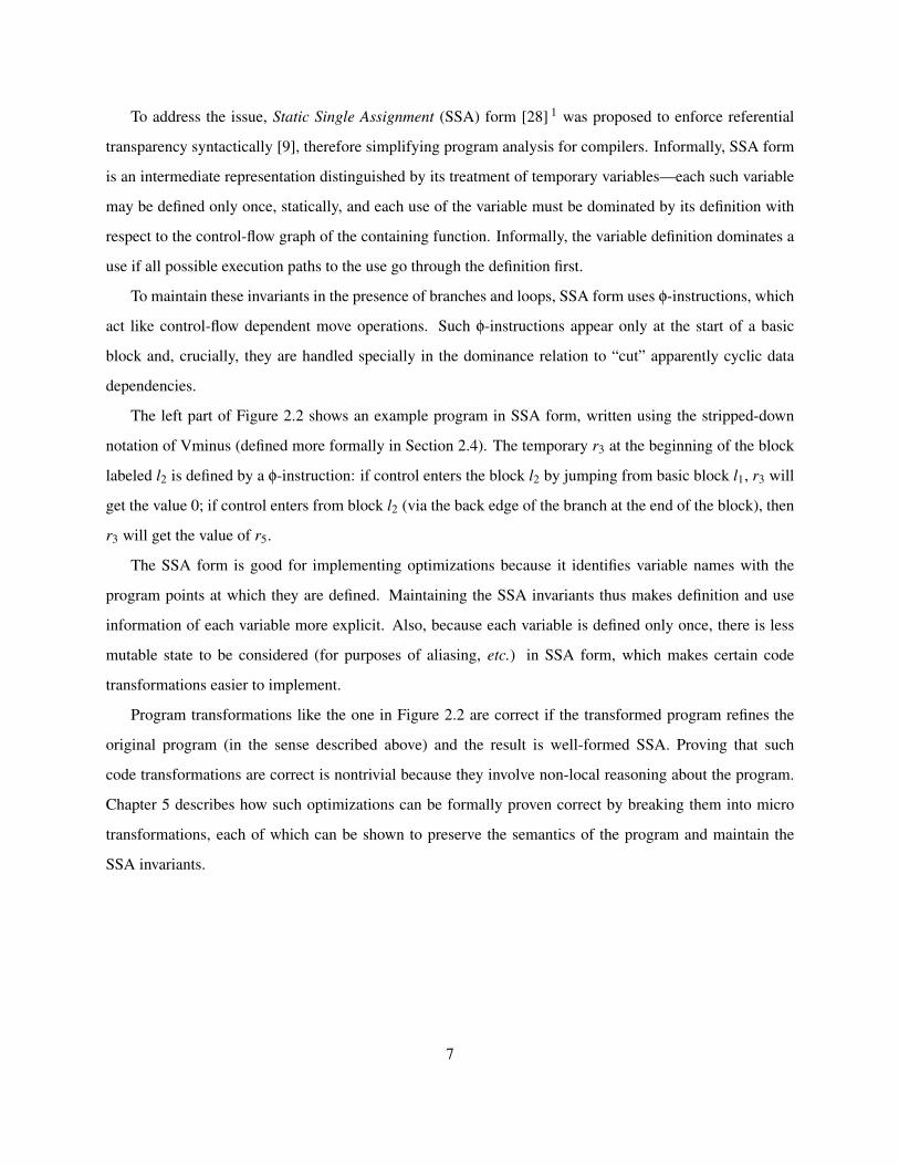
To address the issue, Static Single Assignment (SSA) form [28] 1 was proposed to enforce referential
transparency syntactically [9], therefore simplifying program analysis for compilers. Informally, SSA form
is an intermediate representation distinguished by its treatment of temporary variables—each such variable
may be defined only once, statically, and each use of the variable must be dominated by its definition with
respect to the control-flow graph of the containing function. Informally, the variable definition dominates a
use if all possible execution paths to the use go through the definition first.
To maintain these invariants in the presence of branches and loops, SSA form uses φ-instructions, which
act like control-flow dependent move operations. Such φ-instructions appear only at the start of a basic
block and, crucially, they are handled specially in the dominance relation to “cut” apparently cyclic data
dependencies.
The left part of Figure 2.2 shows an example program in SSA form, written using the stripped-down
notation of Vminus (defined more formally in Section 2.4). The temporary r3 at the beginning of the block
labeled l2 is defined by a φ-instruction: if control enters the block l2 by jumping from basic block l1, r3 will
get the value 0; if control enters from block l2 (via the back edge of the branch at the end of the block), then
r3 will get the value of r5.
The SSA form is good for implementing optimizations because it identifies variable names with the
program points at which they are defined. Maintaining the SSA invariants thus makes definition and use
information of each variable more explicit. Also, because each variable is defined only once, there is less
mutable state to be considered (for purposes of aliasing, etc.) in SSA form, which makes certain code
transformations easier to implement.
Program transformations like the one in Figure 2.2 are correct if the transformed program refines the
original program (in the sense described above) and the result is well-formed SSA. Proving that such
code transformations are correct is nontrivial because they involve non-local reasoning about the program.
Chapter 5 describes how such optimizations can be formally proven correct by breaking them into micro
transformations, each of which can be shown to preserve the semantics of the program and maintain the
SSA invariants.
7
Original Transformed
l1 : · · ·· · ·brr0 l2 l3
l2 :r3 = phi int[0, l1][r5, l2]r4 := r1 ∗ r2r5 := r3 + r4r6 := r5 ≥ 100brr6 l2 l3
l3 :r7 = phi int[0, l1][r5, l2]r8 := r1 ∗ r2r9 := r8 + r7
l1 : · · ·r4 := r1 ∗ r2brr0 l2 l3
l2 :r3 = phi int[0, l1][r5, l2]
r5 := r3 + r4r6 := r5 ≥ 100brr6 l2 l3
l3 :r7 = phi int[0, l1][r5, l2]
r9 := r4 + r7
In the original program (left), r1 ∗ r2 is a partial common expression for the definitions of r4 and r8, becausethere is no domination relation between r4 and r8. Therefore, eliminating the common expression directlyis not correct. For example, we cannot simply replace r8 := r1 ∗ r2 by r8 := r4 since r4 is not available atthe definition of r8 if the block l2 does not execute before l3 runs. To transform this program, we might firstmove the instruction r4 := r1 ∗ r2 from the block l2 to the block l1 because the definitions of r1 and r2 mustdominate l1, and l1 dominates l2. Then we can safely replace all the uses of r8 by r4, because the definitionof r4 in l1 dominates l3 and therefore dominates all the uses of r8. Finally, r8 is removed, because there areno uses of r8.
Figure 2.2: An SSA-based optimization.
C, C++, Haskell, ObjC, ObjC++, Scheme, Scala...
Alpha, ARM, PowerPC, Sparc,
X86, Mips, …
Code Generator/
JITLLVM IR
Optimizations/Transformations
Program analysis
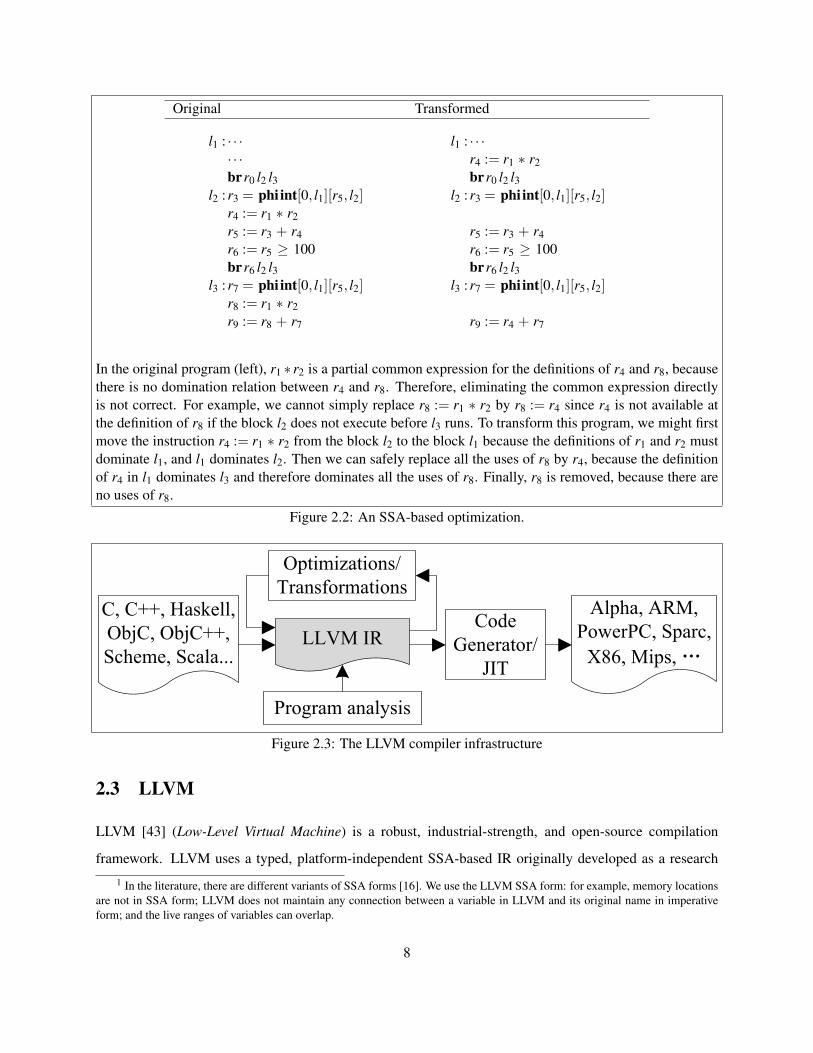
Figure 2.3: The LLVM compiler infrastructure
2.3 LLVM
LLVM [43] (Low-Level Virtual Machine) is a robust, industrial-strength, and open-source compilation
framework. LLVM uses a typed, platform-independent SSA-based IR originally developed as a research
1 In the literature, there are different variants of SSA forms [16]. We use the LLVM SSA form: for example, memory locationsare not in SSA form; LLVM does not maintain any connection between a variable in LLVM and its original name in imperativeform; and the live ranges of variables can overlap.
8
Types typ : : = intConstants cnst : : = IntValues val : : = r | cnstBinops bop : : = + | ∗ | && |= | ≥ | ≤ | · · ·Right-hand-sides rhs : : = val1 bopval2Commands c : : = r := rhsTerminators tmn : : = brval l1 l2 | ret typval
Phi Nodes φ : : = r = phi typ [valj, lj]j
Instructions insn : : = φ | c | tmnNon-φs ψ : : = c | tmnBlocks b : : = lφctmnFunctions f : : = fun{b}
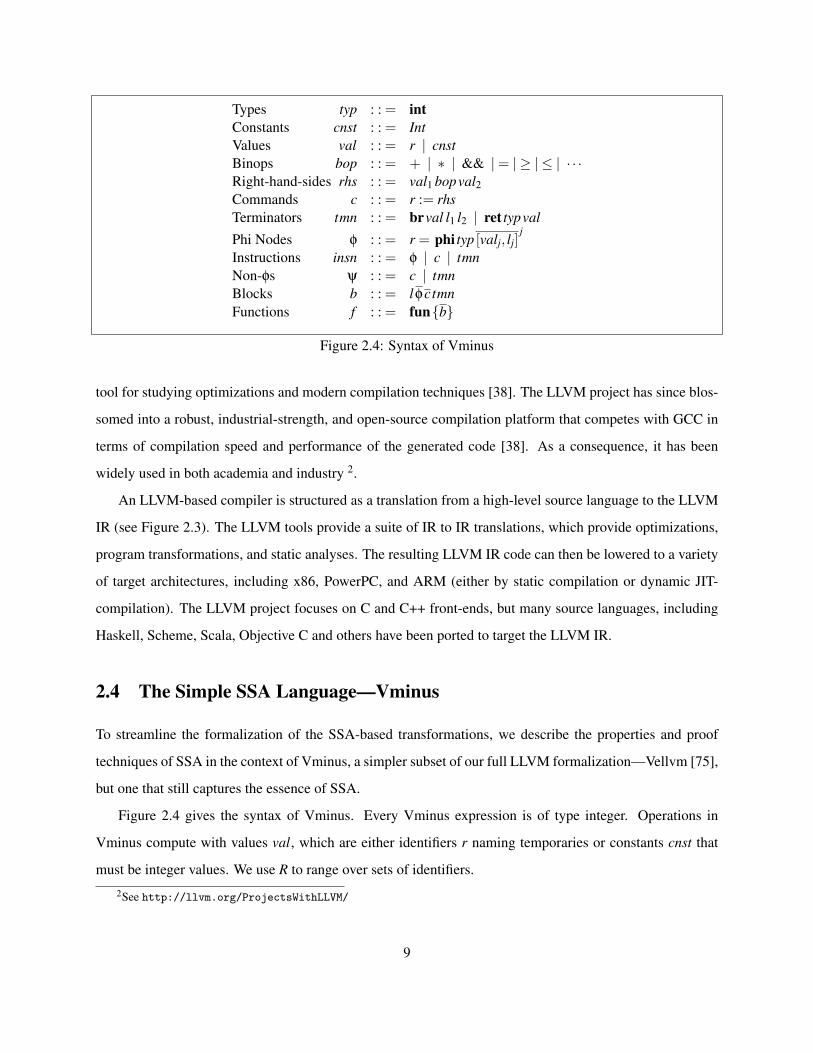
Figure 2.4: Syntax of Vminus
tool for studying optimizations and modern compilation techniques [38]. The LLVM project has since blos-
somed into a robust, industrial-strength, and open-source compilation platform that competes with GCC in
terms of compilation speed and performance of the generated code [38]. As a consequence, it has been
widely used in both academia and industry 2.
An LLVM-based compiler is structured as a translation from a high-level source language to the LLVM
IR (see Figure 2.3). The LLVM tools provide a suite of IR to IR translations, which provide optimizations,
program transformations, and static analyses. The resulting LLVM IR code can then be lowered to a variety
of target architectures, including x86, PowerPC, and ARM (either by static compilation or dynamic JIT-
compilation). The LLVM project focuses on C and C++ front-ends, but many source languages, including
Haskell, Scheme, Scala, Objective C and others have been ported to target the LLVM IR.
2.4 The Simple SSA Language—Vminus
To streamline the formalization of the SSA-based transformations, we describe the properties and proof
techniques of SSA in the context of Vminus, a simpler subset of our full LLVM formalization—Vellvm [75],
but one that still captures the essence of SSA.
Figure 2.4 gives the syntax of Vminus. Every Vminus expression is of type integer. Operations in
Vminus compute with values val, which are either identifiers r naming temporaries or constants cnst that
must be integer values. We use R to range over sets of identifiers.
2See http://llvm.org/ProjectsWithLLVM/
9
All code in Vminus resides in a top-level function, whose body is composed of blocks b. Here, b denotes
a list of blocks; we also use similar notation for other lists. As is standard, a basic block consists of a labeled
entry point l, a series of φ nodes, a list of commands cs, and a terminator instruction tmn. In the following,
we also use the label l of a block to denote the block itself.
Because SSA ensures the uniqueness of variables in a function, we use r to identify instructions that
assign temporaries. For instructions that do not update temporaries, such as terminators, we introduce
“ghost” identifiers to identify them—r : brval l1 l2. Ghost identifiers satisfy uniqueness statically but do not
have dynamic semantics, and are not shown when we do not distinguish instructions.
The set of blocks making up the top-level function constitutes a control-flow graph with a well-defined
entry point that cannot be reached from other blocks. We write f [l] = bbc if there is a block b with label l
in function f . Here, the bc (pronounced “some”) indicates that the function is partial (might return “none”
instead).
As usual in SSA, the φ nodes join together values from a list of predecessor blocks of the control-
flow graph—each φ node takes a list of (value, label) pairs that indicates the value chosen when control
transfers from a predecessor block with the associated label. The commands c include the usual suite of
binary arithmetic or comparison operations (bop—e.g., addition +, multiplication ∗, and &&, equivalence
=, greater than or equal ≥, less than or equal ≤, etc.). We denote the right-hand-sides of commands by
rhs. Block terminators (br and ret) branch to another block or return a value from the function. We also
use metavariable insn to range over φ-nodes, commands and terminators, and non-phinodes ψ to represent
commands and terminators.
10
Chapter 3
Mechanized Verification of Computing
Dominators
One crucial component of SSA-based compilers is computing dominators—on a control-follow-graph, a
node l1 dominates a node l2 if all paths from the entry to l2 must go through l1 [8]. Dominance analysis al-
lows compilers to represent programs in the SSA form [28] (which enables many advanced SSA-based opti-
mizations), optimize loops, analyze memory dependency, and parallelize code automatically, etc. Therefore,
one prerequisite to the formal verification of SSA-based compilers is formalizing computing dominators.
In this chapter, we present the formalization of dominance analysis used in the Vellvm project. To
the best of our knowledge, this is the first mechanized verification of dominator computation for LLVM.
Although the CompCertSSA project [14] also formalized dominance analysis to prove the correctness of a
global value numbering optimization, as we explain in Chapter 10, our results are more general: beyond
soundness, we establish completeness and related metatheory results that can be used in other applications.
Because different styles of formalization may also affect the cost of proof engineering, we also discuss some
tradeoffs in the choices of formalization.
To simplify the formal development, we describe the work in the context of Vminus in this section. The
following sections describe how to extend the work for the full Vellvm. Following LLVM, we distinguish
dominators at the block level and at the instruction level. Given the former one, we can easily compute
the latter one. Therefore, we will focus on the block-level analysis. Section 4.2 discusses the instruction-
level analysis, Section 4.3 shows how to use the dominance analysis to design a type checker for the SSA
11
form, and Chapter 5 describes how to verify SSA-based optimizations by the metatheory of the dominance
analysis.
Concretely, we present the following specific contributions:
1. Section 3.1 gives an abstract and succinct specification of computing dominators at the block level.
2. We instantiate the specification by two algorithms. Section 3.2 shows the standard dominance anal-
ysis [7] (AC). Section 3.3 presents an extension of the standard algorithm [24] (CHK) that is easy to
implement and verify, but still fast. We verify the correctness of both algorithms. In the meanwhile,
we provide a verified depth first search algorithm (Section 3.2.1).
3. Then, Section 3.4 constructs dominator trees that compilers traverse to transform programs.
4. Section 3.6 evaluates performance of the algorithms, and shows that in practice CHK runs nearly as
fast as the sophisticated algorithm used in LLVM.
5. We formalize all the claims of the paper for Vminus and the full Vellvm in Coq (available at http:
//www.cis.upenn.edu/~stevez/vellvm/).
Note that in this chapter we present definitions and proofs in Coq; the later chapters use mathematical
notations.
3.1 The Specification of Computing Dominators
This section first defines dominators in term of the syntax of Vminus, then gives an abstract and succinct
specification of algorithms that compute dominators.
3.1.1 Dominance
The set of blocks making up the top-level function f constitutes a control-flow graph (CFG) G = (e,succs)
where e is the entry point (the first block) of f ; succs maps each label to a list of its successors. On a CFG,
we use G |= l1→∗ l2 to denote a path ρ from l1 to l2, and l ∈ ρ to denote that l is in the path ρ. By wf f
(which Section 4.3 formally defines), we require that a well-formed function must contain an entry point that
cannot be reached from other blocks, all terminators can only branch to blocks within f , and that all labels
in f are unique. In this section, we only consider well-formed functions to streamline the presentation.
12
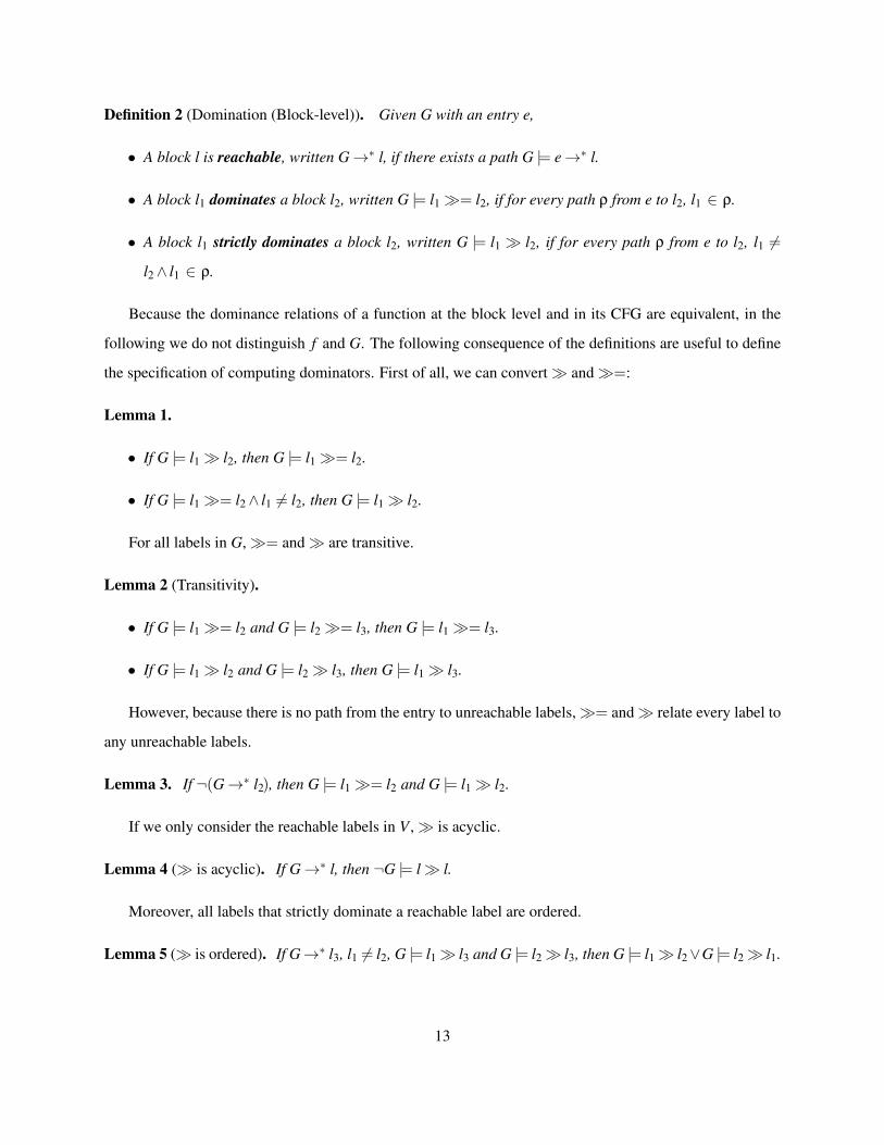
Definition 2 (Domination (Block-level)). Given G with an entry e,
• A block l is reachable, written G→∗ l, if there exists a path G |= e→∗ l.
• A block l1 dominates a block l2, written G |= l1�= l2, if for every path ρ from e to l2, l1 ∈ ρ.
• A block l1 strictly dominates a block l2, written G |= l1 � l2, if for every path ρ from e to l2, l1 6=
l2∧ l1 ∈ ρ.
Because the dominance relations of a function at the block level and in its CFG are equivalent, in the
following we do not distinguish f and G. The following consequence of the definitions are useful to define
the specification of computing dominators. First of all, we can convert� and�=:
Lemma 1.
• If G |= l1� l2, then G |= l1�= l2.
• If G |= l1�= l2∧ l1 6= l2, then G |= l1� l2.
For all labels in G,�= and� are transitive.
Lemma 2 (Transitivity).
• If G |= l1�= l2 and G |= l2�= l3, then G |= l1�= l3.
• If G |= l1� l2 and G |= l2� l3, then G |= l1� l3.
However, because there is no path from the entry to unreachable labels,�= and� relate every label to
any unreachable labels.
Lemma 3. If ¬(G→∗ l2), then G |= l1�= l2 and G |= l1� l2.
If we only consider the reachable labels in V ,� is acyclic.
Lemma 4 (� is acyclic). If G→∗ l, then ¬G |= l� l.
Moreover, all labels that strictly dominate a reachable label are ordered.
Lemma 5 (� is ordered). If G→∗ l3, l1 6= l2, G |= l1� l3 and G |= l2� l3, then G |= l1� l2∨G |= l2� l1.
13
Module Type ALGDOM.
Parameter sdom: f -> l -> set l.
Definition dom f l1 := l1 {+} sdom f l1.
Axiom entry_sound: forall f e, entry f = Some e -> sdom f e = {}.
Axiom successors_sound: forall f l1 l2,
In l1 ((succs f) !!! l2) -> sdom f l1 {<=} dom f l2.
Axiom complete: forall f l1 l2,
wf f -> f |= l1 >> l2 -> l1 ‘in‘ (sdom f l2).
End ALGDOM.
Module AlgDom_Properties(AD: ALGDOM).
Lemma sound: forall f l1 l2,
wf f -> l1 ‘in‘ (AD.sdom f l2) -> f |= l1 >> l2.
(**********************************************************************)
(* Properties: conversion, transitivity, acyclicity, ordering and ... *)
(**********************************************************************)
End AlgDom_Properties.
Figure 3.1: The specification of algorithms that find dominators.
3.1.2 Specification
Coq Notations. We use {} to denote an empty set; use {+}, {<=}, ‘in‘, {\/} and {/\} to denote set
addition, inclusion, membership, union and intersection respectively. Our developments reuse the basic tree
and map data structures implemented in the CompCert project [42]: ATree.t and PTree.t are trees with
keys of type l and positive respectively; PMap.t is a map with keys of type positive. We use ! and !!
to denote tree and map lookup respectively. A tree lookup is partial, while a map lookup returns a default
value when the key to search does not exist. succs are defined by trees. !!! is a special tree lookup for
succs, and it returns an empty list when a searched-for key does not exist. [x] is a list with one element x.
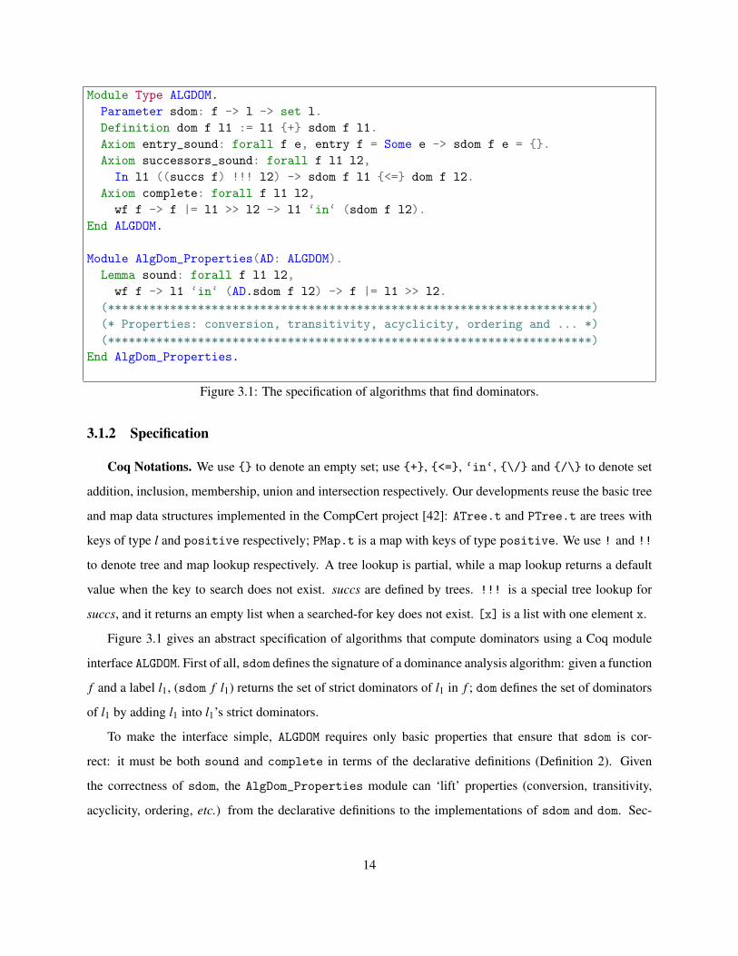
Figure 3.1 gives an abstract specification of algorithms that compute dominators using a Coq module
interface ALGDOM. First of all, sdom defines the signature of a dominance analysis algorithm: given a function
f and a label l1, (sdom f l1) returns the set of strict dominators of l1 in f ; dom defines the set of dominators
of l1 by adding l1 into l1’s strict dominators.
To make the interface simple, ALGDOM requires only basic properties that ensure that sdom is cor-
rect: it must be both sound and complete in terms of the declarative definitions (Definition 2). Given
the correctness of sdom, the AlgDom_Properties module can ‘lift’ properties (conversion, transitivity,
acyclicity, ordering, etc.) from the declarative definitions to the implementations of sdom and dom. Sec-
14
Efficiency
Lengauer-Tarjan (LT, in LLVM and GCC)
Based on graph theory
O(E x log(N))Cooper-Harvey-Kennedy (CHK)
Extended from AC
Nearly as fast as LT in common cases
Verifiability
Allen-Cocke (AC)
Based on Kildall’s algorithm
A large asymptotic complexity
Figure 3.2: Algorithms of computing dominators
tion 3.4, Section 3.5, Section 4.3 and Chapter 8 show how clients of ALGDOM use the properties proven in
AlgDom_Properties by examples.
ALGDOM requires completeness of the algorithm directly. Soundness of the algorithm can be
proven by two more basic properties: entry_sound requires that the entry has no strict dominators;
successors_sound requires that if l1 is a successor of l2, then l2’s dominators must include l1’s strict
dominators. Given an algorithm that establishes the two properties, AlgDom_Properties proves that the
algorithm is sound by induction over any path from the entry to l2.
3.1.3 Instantiations
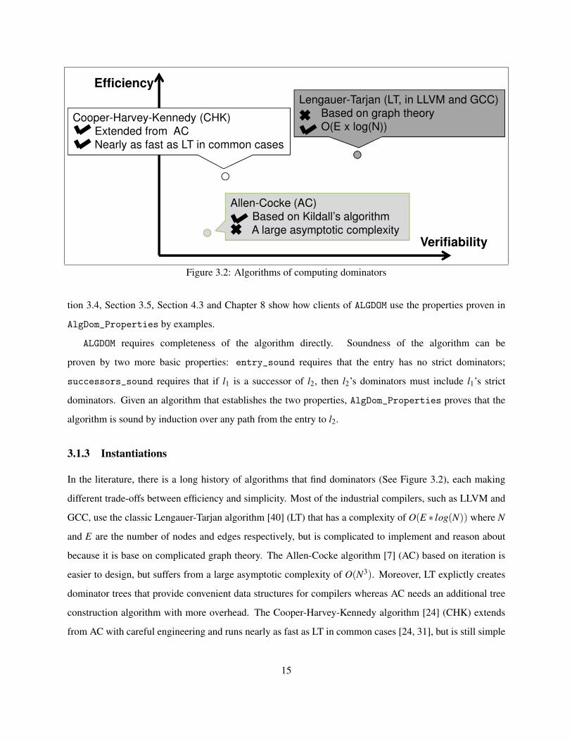
In the literature, there is a long history of algorithms that find dominators (See Figure 3.2), each making
different trade-offs between efficiency and simplicity. Most of the industrial compilers, such as LLVM and
GCC, use the classic Lengauer-Tarjan algorithm [40] (LT) that has a complexity of O(E ∗ log(N)) where N
and E are the number of nodes and edges respectively, but is complicated to implement and reason about
because it is base on complicated graph theory. The Allen-Cocke algorithm [7] (AC) based on iteration is
easier to design, but suffers from a large asymptotic complexity of O(N3). Moreover, LT explictly creates
dominator trees that provide convenient data structures for compilers whereas AC needs an additional tree
construction algorithm with more overhead. The Cooper-Harvey-Kennedy algorithm [24] (CHK) extends
from AC with careful engineering and runs nearly as fast as LT in common cases [24, 31], but is still simple
15

entry
{e,5}
{a,4}
{d,2}
{b,3}
{c,1}
{z,_}
{y,_}
stk visited PO_l2p po
e[a d] ee[d]; a[b] e ae[d]; a[]; b[c d] e a be[d]; a[]; b[d]; c[] e a b c (c,1)e[d]; a[]; b[]; d[b] e a b c d (c,1)e[d]; a[]; b[]; d[] e a b c d (c,1); (d,2)e[d]; a[]; b[]; e a b c d (c,1); (d,2); (b,3)e[d]; a[]; e a b c d (c,1); (d,2); (b,3); (a,4)e[] e a b c d (c,1); (d,2); (b,3); (a,4); (e,5)
Figure 3.3: The postorder (left) and the DFS execution sequence (right).
to implement and reason about. Moreover, CHK generates dominator trees implicitly, and provides a faster
tree construction algorithm.
Because CHK gives a relatively good trade-off between verifiability and efficency, we present CHK
as an instance of ALGDOM. In the following sections, we first review the AC algorithm, and then study its
extension CHK.
3.2 The Allen-Cocke Algorithm
The Allen-Cocke algorithm (AC) is an instance of the forward worklist-based Kildall’s algorithm [35] that
computes program fixpoints by iteration. The number of iterations that a worklist-based algorithm takes to
meet a fixpoint depends on the order in which nodes are processed: in particular, forward algorithms can
converge relatively faster when visiting nodes in reverse postorder (PO) [33].
At the high-level, our Coq implementation of AC works in three steps: 1) calculate the PO of a CFG by
depth-first-search (DFS); 2) compute strict dominators for PO-numbered nodes in Kildall; 3) finally relate
the analysis results to the original nodes. We omit the 3rd step’s proofs here.
This section first presents a verified DFS algorithm that computes PO, then reviews Kildall’s algorithm
as implemented in the CompCert project [42], and finally it studies the implementation and metatheory of
AC.
16

Record PostOrder := mkPO { PO_cnt: positive; PO_l2p: LTree.t positive }.
Record Frame := mkFr { Fr_name: l; Fr_scs: list l }.
Definition dfs_F_type : Type := forall (succs: LTree.t (list l))
(visited: LTree.t unit) (po:PostOrder) (stk: list Frame), PostOrder.
Definition dfs_F (f: dfs_F_type) (succs: LTree.t (list l))
(visited: LTree.t unit) (po:PostOrder) (stk: list Frame): PostOrder :=
match find_next succs visited po stk with
| inr po’ => po’
| inl (next, visited’, po’, stk’) => f succs visited’ po’ stk’
end.
Figure 3.4: The DFS algorithm.
3.2.1 DFS: PO-numbering
DFS starts at the entry, visits nodes as deep as possible along each path, and backtracks when all deep nodes
are visited. DFS generates PO by numbering a node after all its children are numbered. Figure 3.3 gives a
PO-numbered CFG. In the CFG, we represent the depth-first-search (DFS) tree edges by solid arrows, and
non-tree edges by dotted arrows. We draw the entry node in a box, and other nodes in circles. Each node is
labeled by a pair with its original label name on the left, and its PO number on the right. Because DFS only
visits reachable nodes, the PO numbers of unreachable nodes are represented by ‘ ’.
Figure 3.4 shows the data structures and auxiliary functions used by a typical DFS algorithm that
maintains four components to compute PO. PostOrder takes the next available PO number and a map
from nodes to their PO numbers with type positive. The map from a node to its successors is represented
by succs. To facilitate reasoning about DFS, we represent the recursive information of DFS explicitly by a
list of Frame records that each contains a node Fr_name and its unprocessed successors Fr_scs. To prevent
the search from revisiting nodes, the DFS algorithm uses visited to record visited nodes. dfs_F defines
one recursive step of DFS.
Figure 3.3 (on the right) gives a DFS execution sequence (by running dfs_F until all nodes are visited)
of the CFG in Figure 3.3 (on the left) . We use l[l1 · · · ln] to denote a frame with the node l and its unprocessed
successors l1 to ln; (l, p) to denote a node l and its PO p. Initially the DFS adds the entry and its successors
to the stack. At each recursive step, find_next finds the next available node that is the unvisited node in
the Fr_scs of the latest node l′ of the stack. If the next available node exists, the DFS pushes the node with
17
Fixpoint iter (A:Type) (n:nat) (F:A->A) (g:A) : A :=
match n with
| O => g
| S p => F (iter A p F g)
end.
Definition wf_stk succs visited stk :=
stk_in_succs succs stk /\ incl visited succs
Program Fixpoint dfs_tmn succs visited po stk
(Hp: wf_stk succs visited stk) {measure (size succs - size visited)}:
{ po’:PostOrder | exists p:nat,
forall k (Hlt: p < k) (g:dfs_F_type),
iter _ k dfs_F g succs visited po stk = po’ } :=
match find_next succs visited po stk with
| inr po’ => po’
| inl (next, visited’, po’, stk’) =>
let _ := dfs_tmn succs visited’ po’ stk’ _ in _
end.
Program Definition dfs succs entry : PostOrder :=
fst (dfs_tmn succs empty (mkPO 1 empty) (mkFr entry [(succs!!!entry)]) _).
Figure 3.5: Termination of the DFS algorithm.
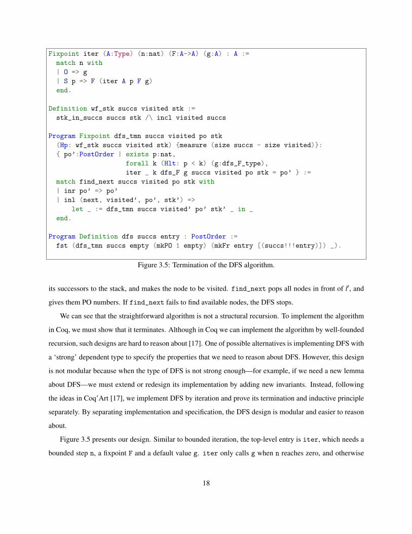
its successors to the stack, and makes the node to be visited. find_next pops all nodes in front of l′, and
gives them PO numbers. If find_next fails to find available nodes, the DFS stops.
We can see that the straightforward algorithm is not a structural recursion. To implement the algorithm
in Coq, we must show that it terminates. Although in Coq we can implement the algorithm by well-founded
recursion, such designs are hard to reason about [17]. One of possible alternatives is implementing DFS with
a ‘strong’ dependent type to specify the properties that we need to reason about DFS. However, this design
is not modular because when the type of DFS is not strong enough—for example, if we need a new lemma
about DFS—we must extend or redesign its implementation by adding new invariants. Instead, following
the ideas in Coq’Art [17], we implement DFS by iteration and prove its termination and inductive principle
separately. By separating implementation and specification, the DFS design is modular and easier to reason
about.
Figure 3.5 presents our design. Similar to bounded iteration, the top-level entry is iter, which needs a
bounded step n, a fixpoint F and a default value g. iter only calls g when n reaches zero, and otherwise
18
recursively calls one more iteration of F. If F is terminating, we can prove that there must exist a final value
and a bound n, such that for any bound k that is greater than or equal to n, iter always stops and generates
the same final value. In other words, F must reach a fixpoint with less than n steps. In fact, the proof of the
existence of n is erasable; the computation part of the proof provides a terminating algorithm for free, not
requiring the bound step at runtime.
Figure 3.5 proves that the DFS must terminate, as shown by dfs_tmn, which is implemented by well-
founded recursion over the number of unvisited nodes. Intuitively, this follows because after each iteration,
the DFS visits more nodes. The invariant that the number of unvisited nodes decreases holds only for well-
formed recursion states (wf_stk), which requires that all visited nodes and unprocessed nodes in frames
must be in the CFG. We implemented dfs_tmn by Coq’s Program Fixpoint, which allows programmers
to leave holes for which Program Fixpoint automatically generates obligations to solve. Using dfs_tmn,
dfs defines the final definition of DFS.
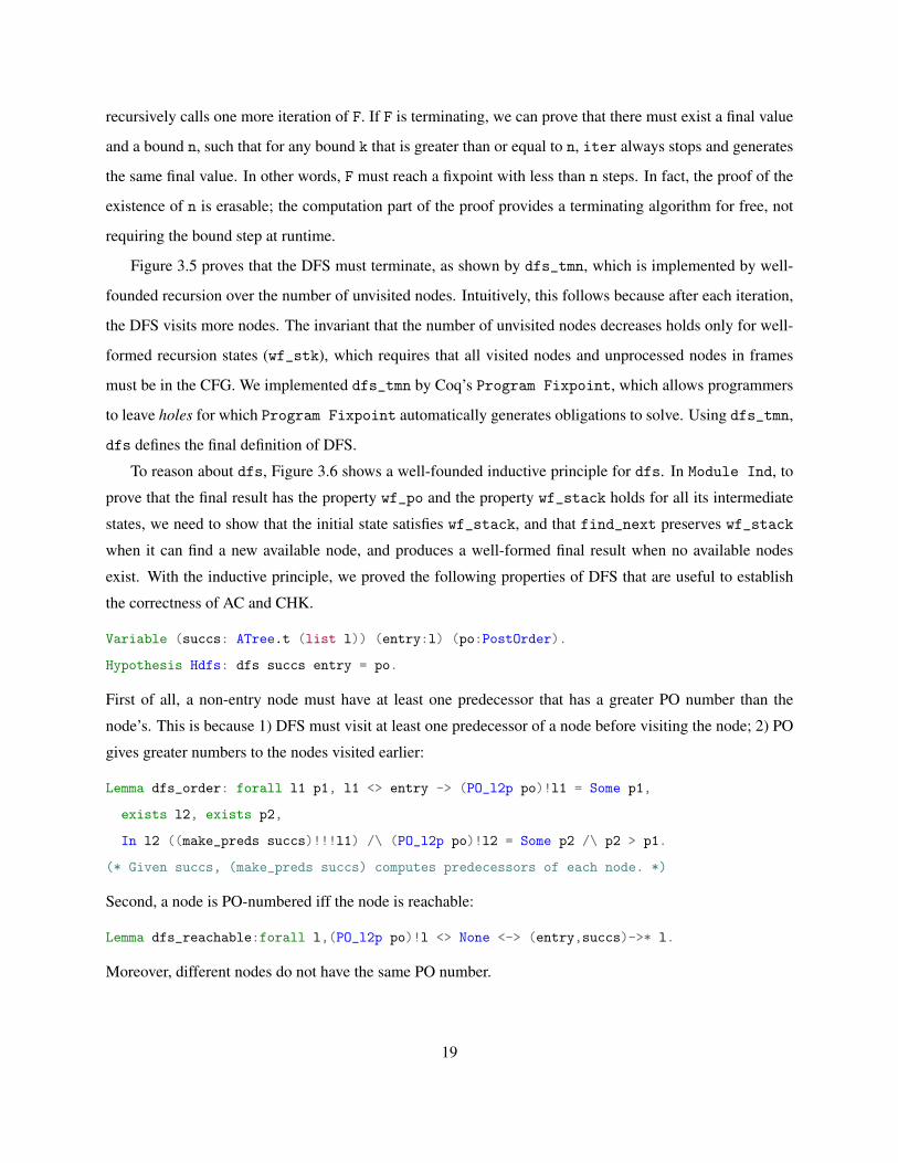
To reason about dfs, Figure 3.6 shows a well-founded inductive principle for dfs. In Module Ind, to
prove that the final result has the property wf_po and the property wf_stack holds for all its intermediate
states, we need to show that the initial state satisfies wf_stack, and that find_next preserves wf_stack
when it can find a new available node, and produces a well-formed final result when no available nodes
exist. With the inductive principle, we proved the following properties of DFS that are useful to establish
the correctness of AC and CHK.
Variable (succs: ATree.t (list l)) (entry:l) (po:PostOrder).
Hypothesis Hdfs: dfs succs entry = po.
First of all, a non-entry node must have at least one predecessor that has a greater PO number than the
node’s. This is because 1) DFS must visit at least one predecessor of a node before visiting the node; 2) PO
gives greater numbers to the nodes visited earlier:
Lemma dfs_order: forall l1 p1, l1 <> entry -> (PO_l2p po)!l1 = Some p1,
exists l2, exists p2,
In l2 ((make_preds succs)!!!l1) /\ (PO_l2p po)!l2 = Some p2 /\ p2 > p1.
(* Given succs, (make_preds succs) computes predecessors of each node. *)
Second, a node is PO-numbered iff the node is reachable:
Lemma dfs_reachable:forall l,(PO_l2p po)!l <> None <-> (entry,succs)->* l.
Moreover, different nodes do not have the same PO number.
19
Module Ind.
Section Ind.
Variable (succs: ATree.t (list l)) (entry:l) (po:PostOrder).
Hypothesis find_next__wf_stack: forall ... (Hwf: wf_stack visited po stk)
(Heq: find_next succs visited po stk = inl (next, visited’, po’, stk’)),
wf_stack visited’ po’ stk’.
Hypothesis wf_stack__find_next__wf_order: forall ...,
(Hwf: wf_stack visited po1 stk)
(Heq: find_next succs visited po1 stk = inr po2), wf_po po2.
Hypothesis entry__wf_stack:
wf_stack empty (mkPO 1 empty) (mkFr entry [(succs!!!entry)]).
Lemma dfs_wf: dfs succs entry = po -> wf_po po.
End Ind.
End Ind.
Figure 3.6: Inductive principle of the DFS algorithm.
Lemma dfs_inj: forall l1 l2 p,
(PO_l2p po)!l2 = Some p -> (PO_l2p po)!l1 = Some p -> l1 = l2.
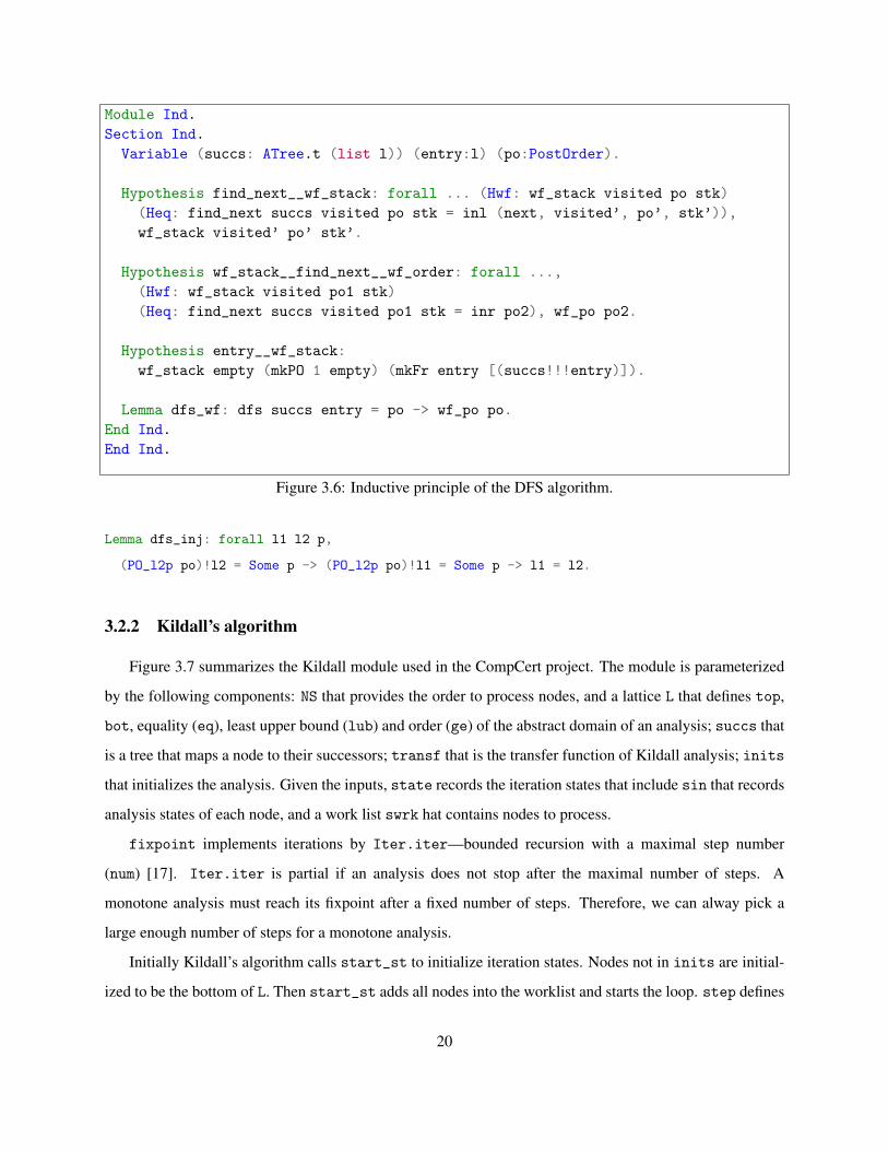
3.2.2 Kildall’s algorithm
Figure 3.7 summarizes the Kildall module used in the CompCert project. The module is parameterized
by the following components: NS that provides the order to process nodes, and a lattice L that defines top,
bot, equality (eq), least upper bound (lub) and order (ge) of the abstract domain of an analysis; succs that
is a tree that maps a node to their successors; transf that is the transfer function of Kildall analysis; inits
that initializes the analysis. Given the inputs, state records the iteration states that include sin that records
analysis states of each node, and a work list swrk hat contains nodes to process.
fixpoint implements iterations by Iter.iter—bounded recursion with a maximal step number
(num) [17]. Iter.iter is partial if an analysis does not stop after the maximal number of steps. A
monotone analysis must reach its fixpoint after a fixed number of steps. Therefore, we can alway pick a
large enough number of steps for a monotone analysis.
Initially Kildall’s algorithm calls start_st to initialize iteration states. Nodes not in inits are initial-
ized to be the bottom of L. Then start_st adds all nodes into the worklist and starts the loop. step defines
20

Module Kildall (NS: PNODE_SET) (L: LATTICE).
Section Kildall.
Variable succs: PTree.t (list positive).
Variable transf : positive -> L.t -> L.t.
Variable inits: list (positive * L.t).
Record state : Type := mkst { sin: PMap.t L.t; swrk: NS.t }.
Definition start_st := mkst (start_state_in inits) (NS.init succs).
Definition propagate_succ (out: L.t) (s: state) (n: positive) :=
let oldl := s.(sin) !! n in
let newl := L.lub oldl out in
if L.eq newl oldl
then mkst (PMap.set n newl s.(sin)) (NS.add n s.(swrk)) else s.
Definition step (s: state): PMap.t L.t + state :=
match NS.pick s.(swrk) with
| None => inl s.(sin)
| Some(n, rem) => inr (fold_left
(propagate_succ (transf n s.(sin) !! n))
(succs !!! n) (mkst s.(sin) rem))
end.
Variable num : positive.
Definition fixpoint : option (PMap.t L.t):= Iter.iter step num start_st.
End Kildall.
End Kildall.
Figure 3.7: Kildall’s algorithm.
the loop body. At step, Kildall’s algorithm checks if there are still unprocessed nodes in the worklist. If the
worklist is empty, the algorithm stops. Otherwise, step picks a node from the worklist in term of the order
provided by NS, and then propagates its information (computed by transf) to all the node’s successors by
propagate_succ. In propagate_succ, the new value of a successor is L.lub of its old value and the
propagated value from its predecessor. The algorithm only adds a successor into the worklist when its value
is changed.
Kildall’s algorithm satisfies the following properties:
21
Variable res: PMap.t L.t.
Hypothesis Hfix: fixpoint = Some res.
First of all, the worklist contains nodes that have unstable successors in the current state. Formally, each
state st preserves the following invariant:
forall n, NS.In n st.(swrk) \/
(forall s, In s (succs!!!n) -> L.ge st.(sin)!!s (transf n st.(sin)!!n)).
Each iteration may only remove the picked node n from the worklist. If none of n’s successors’ values
are changed, no matter whether n belongs to its successors, n won’t be added back to the worklist. There-
fore, the above invariant holds. This invariant implies that when the analysis stops, all nodes hold the
in-equations:
Lemma fixpoint_solution: forall s,
In s (succs!!!n) -> L.ge res!!s (transf n res!!n).
The second property of Kildall’s algorithm is monotonicity. At each iteration, the value of a successor of the
picked node can only be updated from oldl to newl. Because newl is the least upper bound of oldl and
out, newl is greater than or equal to oldl. Therefore, iteration states are always monotonic:
Lemma fixpoint_mono: incr (start_state_in inits) res.
where incr is a pointwise lift of L.ge for corresponding nodes. In particular, the final states must be greater
than or equal to the initial states. When an iteration does not change states, no nodes will be added back to
the worklist, but the size of worklist must decrease. Therefore, a monotonic analysis must reach its fixpoint
with less than N2 ∗H steps where N is the number of nodes; H is the height of the lattice of the analysis [33].
3.2.3 The AC algorithm
AC instantiates Kildall with PN that picks nodes in reverse PO (by picking the maximal nodes from the
worklist), and LDoms that defines the lattice of AC. Dominance analysis computes a set of strict dominators
for each node. We represent the domain of LDoms by option (set l). The top and bot of LDoms are
Some nil and None respectively. The least upper bound, order and equality of LDoms are lifted from set
intersection, set inclusion, and set equality to option: None is smaller than Some x for any x. This design
leads to better performance by providing shortcuts for operations on None. Note that using None as bot
does not make the height of LDoms to be infinite, because any non-bot element can only contain nodes in
the CFG, and the height of LDoms is N.
AC uses the following transfer function and initialization:
22
Definition transf l1 input := l1 {+} input.
Definition inits := [(e, LDoms.top)].
Initially AC sets the strict dominators of the entry to be empty, and other nodes’ strict dominators to be all
labels in the function. The algorithm will iteratively remove non-strict-dominators from the sets until the
conditions below hold (by Lemma fixpoint_mono and Lemma fixpoint_solution):
(forall s, In s (succs!!!n) ->
L.ge (st.(sin))!!s (n{+}(st.(sin))!!n)) /\ (st.(sin))!!e = {}.
which proves that AC satisfies entry_sound and successors_sound.
To show that the algorithm is complete, it is sufficient to show that each iteration state st preserves the
following invariant:
forall n1 n2, ~ n1 ‘in‘ st.(sin)!!n2 -> ~ (e, succs) |= n1 >> n2.
In other words, AC only removes non-strict dominators. Initially, AC sets the entry’s strict dominators
to be empty. Because in a well-formed CFG, the entry has no predecessors, the invariant holds at the
very beginning. At each iteration, suppose that we pick a node n and update one of its successors s.
Consider a node n’ not in LDoms.lub st.(sin)!!s (n {+} st.(sin)!!n). If n’ is not in LDoms.lub
st.(sin)!!s, then n’ does not strictly dominate s because st holds the invariant. If n’ is not in (n {+}
st.(sin)!!n), then n’ does not strictly dominate n because st holds the invariant. Appending the path
from the entry to n that bypasses n’ with the edge from n to s leads to a path from the entry to s that
bypasses n’. Therefore, n’ does not strictly dominate s, either.
3.3 Extension: the Cooper-Harvey-Kennedy Algorithm
The CHK algorithm is based on the following observation: when AC processes nodes in a reversed post-
order (PO), if we represent the set of strict dominators in a list, and always add a newly discovered strict
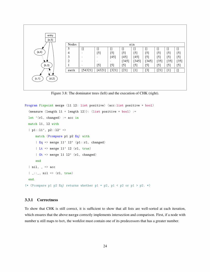
dominator at the head of the list (on the left in Figure 3.8), the list must be sorted by PO. Figure 3.8 (on the
right) shows the execution of the algorithm for the CFG in Figure 3.3.
Because lists of strict dominators are always sorted, we can implement the set intersection (lub) and the
set comparison (eq) of two sorted lists by traversing the two lists only once. Moreover, the algorithm only
calls eq after lub. Therefore, we can group lub and eq into LDoms.lub together. The following defines
a merge function used by LDoms.lub that intersects two sorted lists and returns whether the final result
equals to the left one:
23
entry
{e,5}
{a,4}
{b,3}
{d,2}{c,1}
Nodes sin
5 [] [] [] [] [] [] [] [] []4 · [5] [5] [5] [5] [5] [5] [5] [5]3 · · [45] [45] [45] [5] [5] [5] [5]2 · · · [345] [345] [345] [35] [35] [35]1 · [5] [5] [5] [5] [5] [5] [5] [5]swrk [54321] [4321] [321] [21] [1] [3] [21] [1] []
Figure 3.8: The dominator trees (left) and the execution of CHK (right).
Program Fixpoint merge (l1 l2: list positive) (acc:list positive * bool)
{measure (length l1 + length l2)}: (list positive * bool) :=
let ’(rl, changed) := acc in
match l1, l2 with
| p1::l1’, p2::l2’ =>
match (Pcompare p1 p2 Eq) with
| Eq => merge l1’ l2’ (p1::rl, changed)
| Lt => merge l1’ l2 (rl, true)
| Gt => merge l1 l2’ (rl, changed)
end
| nil, _ => acc
| _::_, nil => (rl, true)
end.
(* (Pcompare p1 p2 Eq) returns whether p1 = p2, p1 < p2 or p1 > p2. *)
3.3.1 Correctness
To show that CHK is still correct, it is sufficient to show that all lists are well-sorted at each iteration,
which ensures that the above merge correctly implements intersection and comparison. First, if a node with
number n still maps to bot, the worklist must contain one of its predecessors that has a greater number.
24
forall n, in_cfg n succs -> (st.(sin))!!n = None ->
exists p, In p ((make_preds succs)!!!n) /\ p > n /\ PN.In p st.(st_wrk).
(* in_cfg checks if a node is in CFG. *)
This invariant holds in the beginning because all nodes are in the worklist. At each iteration, the invariant
implies that the picked node n with the maximal number in st.(st_wrk) is not bot. Suppose it is bot,
there cannot be any node with greater number in the worklist. This property ensures that after each iteration,
the successors of n cannot be bot, and that the new nodes added into the worklist cannot be bot, because
they must be those successors. Therefore, the predecessors of the remaining bot nodes still in the worklist
cannot be n. Since only n is removed, the rest of the bot nodes still hold the above invariant.
In the algorithm, a node’s value is changed from bot to non-bot when one of its non-bot predecessors
is processed. With the above invariant, we know that the predecessor must be of larger number. Once a node
turns to be non-bot, no new elements will be added in its set. Therefore, this implies that, at each iteration,
if the value of a node is not bot, then all its candidate strict dominators must be larger than the node:
forall n sdms, (st.(sin))!!n = Some sdms -> Forall (Plt n) sdms.
(* Plt is the less-than of positive. *)
Moreover, a node n is considered as a candidate of strict dominators originally by tranf that always
cons n at the head of (st.(sin))!!n. Therefore, we proved that the non-bot value of a node is always
sorted:
forall n sdms, (st.(sin))!!n = Some sdms -> Sorted Plt (n::sdms).
3.4 Constructing Dominator Trees
In practice, compilers construct dominator trees from dominators, and analyze or optimize programs by
recursion on dominator trees.
Definition 3.
• A block l1 is an immediate dominator of a block l2, written G |= l1 ≫ l2, if G |= l1 � l2 and
(∀G |= l3� l2,G |= l3�= l1).
• A tree is called a dominator tree of G if the tree has an edge from l to l′ iff G |= l≫ l′.
Figure 3.8 shows the dominator tree of the CFG in Figure 3.3. In Figure 3.8, solid edges represent tree
edges, and dotted edges represent non-tree but CFG edges.
25
Inductive DTree : Set :=
| DT_node : l -> DTrees -> DTree
with DTrees : Set :=
| DT_nil : DTrees
| DT_cons : l -> DTrees -> DTrees.
Variable (f: function) (entry:l).
Inductive wf_dtree : DTree -> Prop :=
| Wf_DT_node : forall l0 dts (Hrd: f |= entry ->* l0)
(Hnotin: ~ l0 ‘in‘ (dtrees_dom dts)) (Hdisj: disjoint_dtrees dts)
(Hidom: forall_children idom l0 dts) (Hwfdts: wf_dtrees dts),
wf_dtree (DT_node l0 dts)
(* (dtrees_dom dts) returns all labels in dts. *)
(* (disjoint_dtrees dts) ensures that labels of dts are disjointed. *)
(* (forall_children idom l0 dts)) checks that l0 immediate-dominates all *)
(* roots of dts. *)
with wf_dtrees : DTrees -> Prop :=
| Wf_DT_nil : wf_dtrees DT_nil
| Wf_DT_cons : forall dt dts (Hwfdt: wf_dtree dt) (Hwfdts: wf_dtrees dts),
wf_dtrees (DT_cons dt dts).
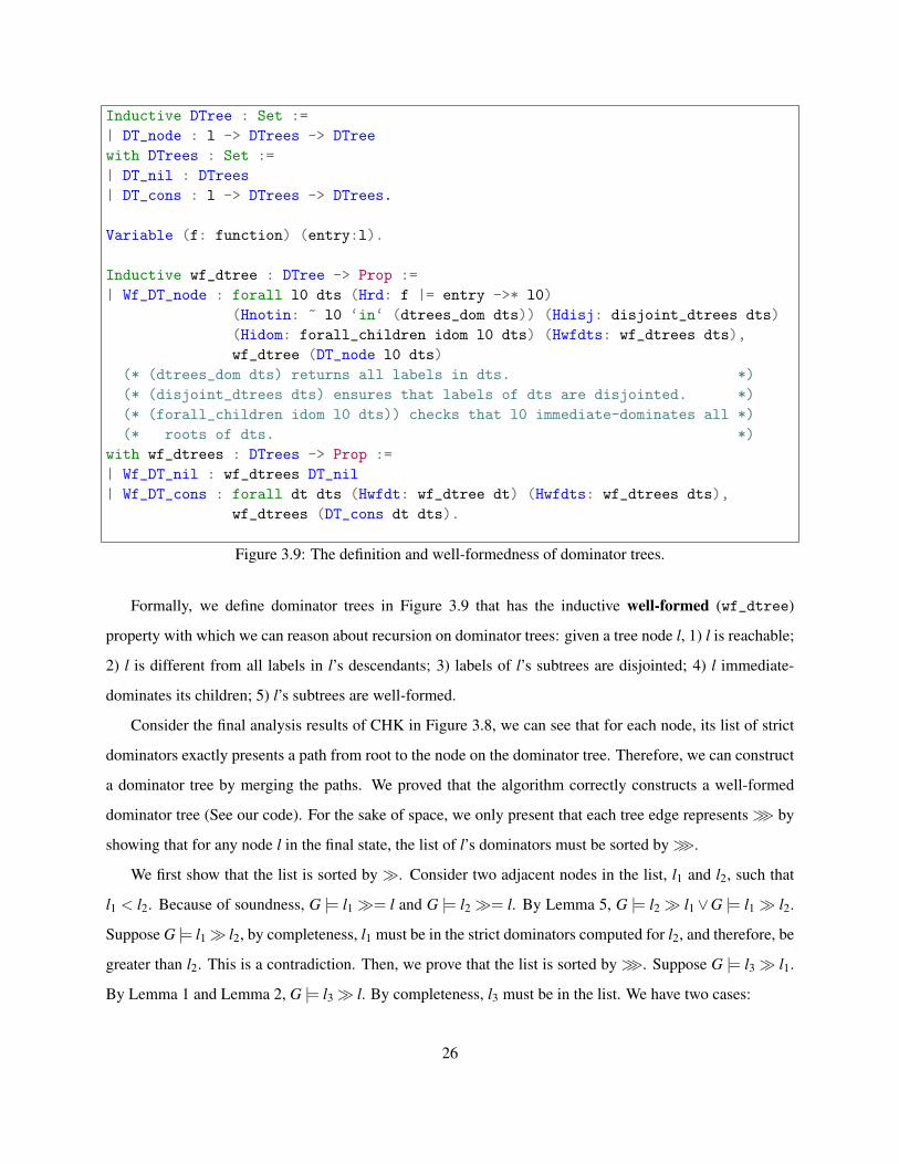
Figure 3.9: The definition and well-formedness of dominator trees.
Formally, we define dominator trees in Figure 3.9 that has the inductive well-formed (wf_dtree)
property with which we can reason about recursion on dominator trees: given a tree node l, 1) l is reachable;
2) l is different from all labels in l’s descendants; 3) labels of l’s subtrees are disjointed; 4) l immediate-
dominates its children; 5) l’s subtrees are well-formed.
Consider the final analysis results of CHK in Figure 3.8, we can see that for each node, its list of strict
dominators exactly presents a path from root to the node on the dominator tree. Therefore, we can construct
a dominator tree by merging the paths. We proved that the algorithm correctly constructs a well-formed
dominator tree (See our code). For the sake of space, we only present that each tree edge represents≫ by
showing that for any node l in the final state, the list of l’s dominators must be sorted by≫.
We first show that the list is sorted by�. Consider two adjacent nodes in the list, l1 and l2, such that
l1 < l2. Because of soundness, G |= l1�= l and G |= l2�= l. By Lemma 5, G |= l2� l1∨G |= l1� l2.
Suppose G |= l1� l2, by completeness, l1 must be in the strict dominators computed for l2, and therefore, be
greater than l2. This is a contradiction. Then, we prove that the list is sorted by≫. Suppose G |= l3� l1.
By Lemma 1 and Lemma 2, G |= l3� l. By completeness, l3 must be in the list. We have two cases:
26
1. l3 ≥ l2: Because the list is sorted by�, G |= l3�= l2.
2. l3 ≤ l1: Similarly, G |= l1�= l3. This is a contradiction by Lemma 4.
3.5 Dominance Frontier
Another application of computing dominators is the calculation of dominance frontiers that has applications
to SSA construction algorithms, computing control dependence, and etc.
Cytron et al. define the dominance frontier of a node, b, as:
... the set of all CFG nodes, y, such that b dominates a predecessor of y but does not strictlydominate y [28].
They propose finding the dominance frontier set for each node in a two step manner. They begin by walking
over the dominator tree in a bottom-up traversal. At each node, b, they add to b’s dominance-frontier set any
CFG successors not dominated by b. They then traverse the dominance-frontier sets of b’s dominator-tree
children each member of these frontiers that is not dominated by b is copied into b’s dominance frontier.
We follow an algorithm designed by Cooper, Harvey and Kennedy [24] that approaches the problem
from the opposite direction, and tends to run faster than Cytron et al.’s algorithm in practice. The algorithm
is based on three observations. First, nodes in a dominance frontier represent join points in the graph, nodes
into which control flows from multiple predecessors. Second, the predecessors of any join point, j, must
have j in their respective dominance-frontier sets, unless the predecessor dominates j. This is a direct result
of the definition of dominance frontiers, above. Finally, the dominators of j’s predecessors must themselves
have j in their dominance-frontier sets unless they also dominate j.
These observations lead to a simple algorithm. First, we identify each join point, j—any node with
more than one incoming edge is a join point. We then examine each predecessor, p, of j and walk up
the dominator tree starting at p. We stop the walk when we reach j’s immediate dominator— j is in the
dominance frontier of each of the nodes in the walk, except for j’s immediate dominator. Intuitively, all of
the rest of j’s dominators are shared by j’s predecessors as well. Since they dominate j, they will not have
j in their dominance frontiers.
As shown previously [24], this approach tends to run faster than Cytron et al..’s algorithm in practice,
almost certainly for two reasons. First, the iterative algorithm has already built the dominator tree. Second,
27
0%
50%
100%
150%
200%
250%O
verh
ead
over
LL
VM
CHK-tree
CHK
AC-tree
AC
gocompress ijpeg gzip vpr
mesa artammp
equake256.bzip2
parsertwolf
401.bzip2 gcc mcfhmmer
libquantum lbm milc sjengh264ref
Geo. mean
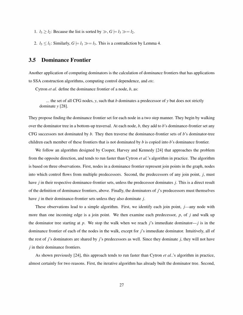
Figure 3.10: Analysis overhead over LLVM’s dominance analysis for our extracted analysis.
the algorithm uses no more comparisons than are strictly necessary. Section 8.5.2 will revisit the implemen-
tation of the algorithm.
3.6 Performance Evaluation
As we discussed, computing dominators is crucial in SSA-based compilers. Therefore, we use the Coq
extraction to obtain a certified implementation of AC and CHK and evaluate the performance of the resultant
code on a 1.73 GHz Intel Core i7 processor with 8 GB memory running benchmarks selected from the SPEC
CPU benchmark suite that consist of over 873k lines of C source code.
Figure 3.10 reports the analysis time overhead (smaller is better) over the C++ version of LLVM dom-
inance analysis (which uses LT) baseline. LT only generates dominator trees. Given a dominator tree, the
strict dominators of a tree node are all the node’s ancestors. The second left bar of each group shows the
overhead of CHK, which provides an average overhead of 27%. The right-most bar of each group is the
overhead of AC, which provides 36% on average.
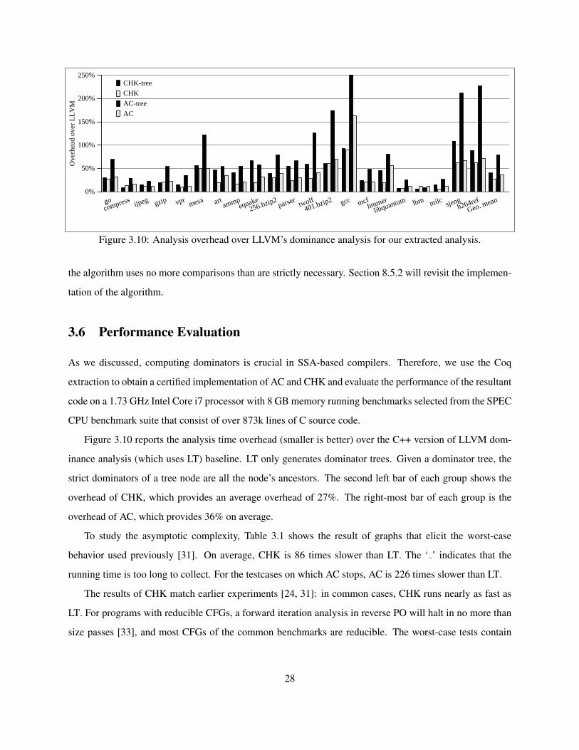
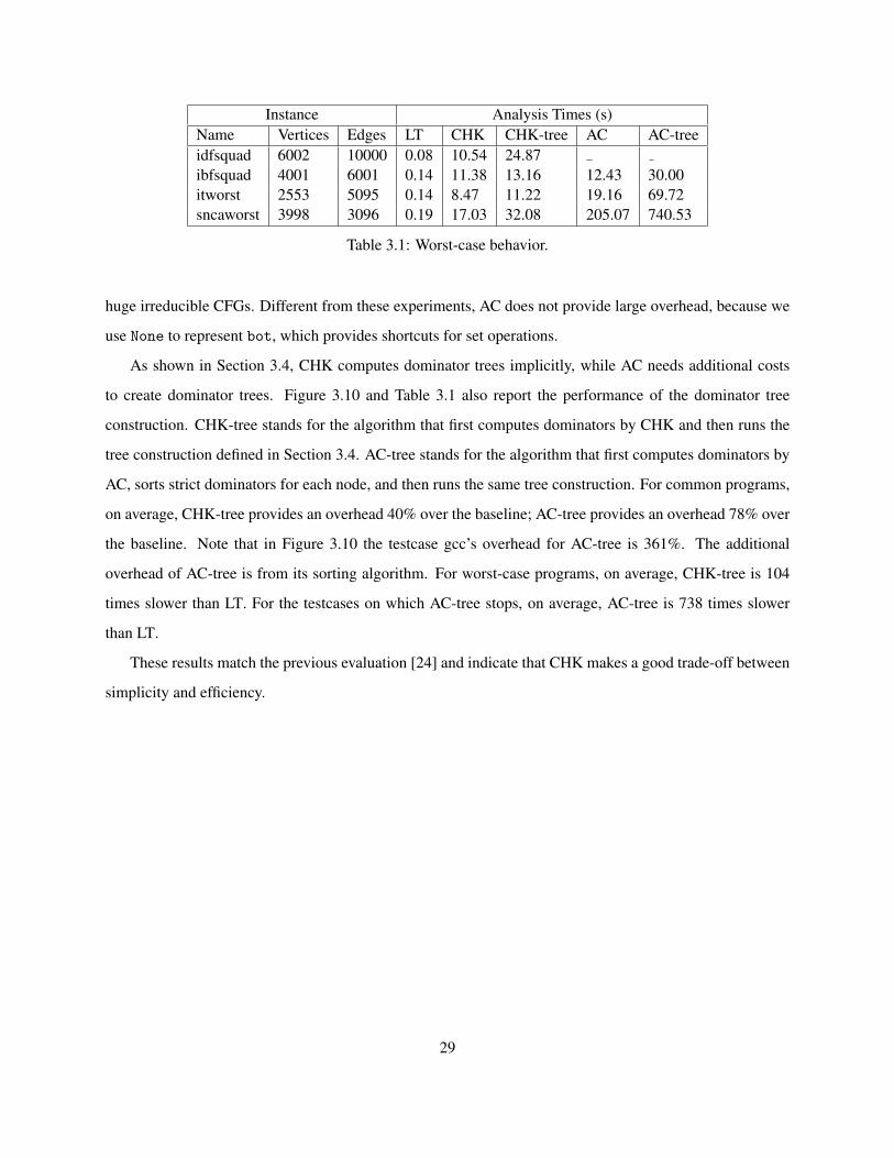
To study the asymptotic complexity, Table 3.1 shows the result of graphs that elicit the worst-case
behavior used previously [31]. On average, CHK is 86 times slower than LT. The ‘ ’ indicates that the
running time is too long to collect. For the testcases on which AC stops, AC is 226 times slower than LT.
The results of CHK match earlier experiments [24, 31]: in common cases, CHK runs nearly as fast as
LT. For programs with reducible CFGs, a forward iteration analysis in reverse PO will halt in no more than
size passes [33], and most CFGs of the common benchmarks are reducible. The worst-case tests contain
28
Instance Analysis Times (s)Name Vertices Edges LT CHK CHK-tree AC AC-treeidfsquad 6002 10000 0.08 10.54 24.87ibfsquad 4001 6001 0.14 11.38 13.16 12.43 30.00itworst 2553 5095 0.14 8.47 11.22 19.16 69.72sncaworst 3998 3096 0.19 17.03 32.08 205.07 740.53
Table 3.1: Worst-case behavior.
huge irreducible CFGs. Different from these experiments, AC does not provide large overhead, because we
use None to represent bot, which provides shortcuts for set operations.
As shown in Section 3.4, CHK computes dominator trees implicitly, while AC needs additional costs
to create dominator trees. Figure 3.10 and Table 3.1 also report the performance of the dominator tree
construction. CHK-tree stands for the algorithm that first computes dominators by CHK and then runs the
tree construction defined in Section 3.4. AC-tree stands for the algorithm that first computes dominators by
AC, sorts strict dominators for each node, and then runs the same tree construction. For common programs,
on average, CHK-tree provides an overhead 40% over the baseline; AC-tree provides an overhead 78% over
the baseline. Note that in Figure 3.10 the testcase gcc’s overhead for AC-tree is 361%. The additional
overhead of AC-tree is from its sorting algorithm. For worst-case programs, on average, CHK-tree is 104
times slower than LT. For the testcases on which AC-tree stops, on average, AC-tree is 738 times slower
than LT.
These results match the previous evaluation [24] and indicate that CHK makes a good trade-off between
simplicity and efficiency.
29
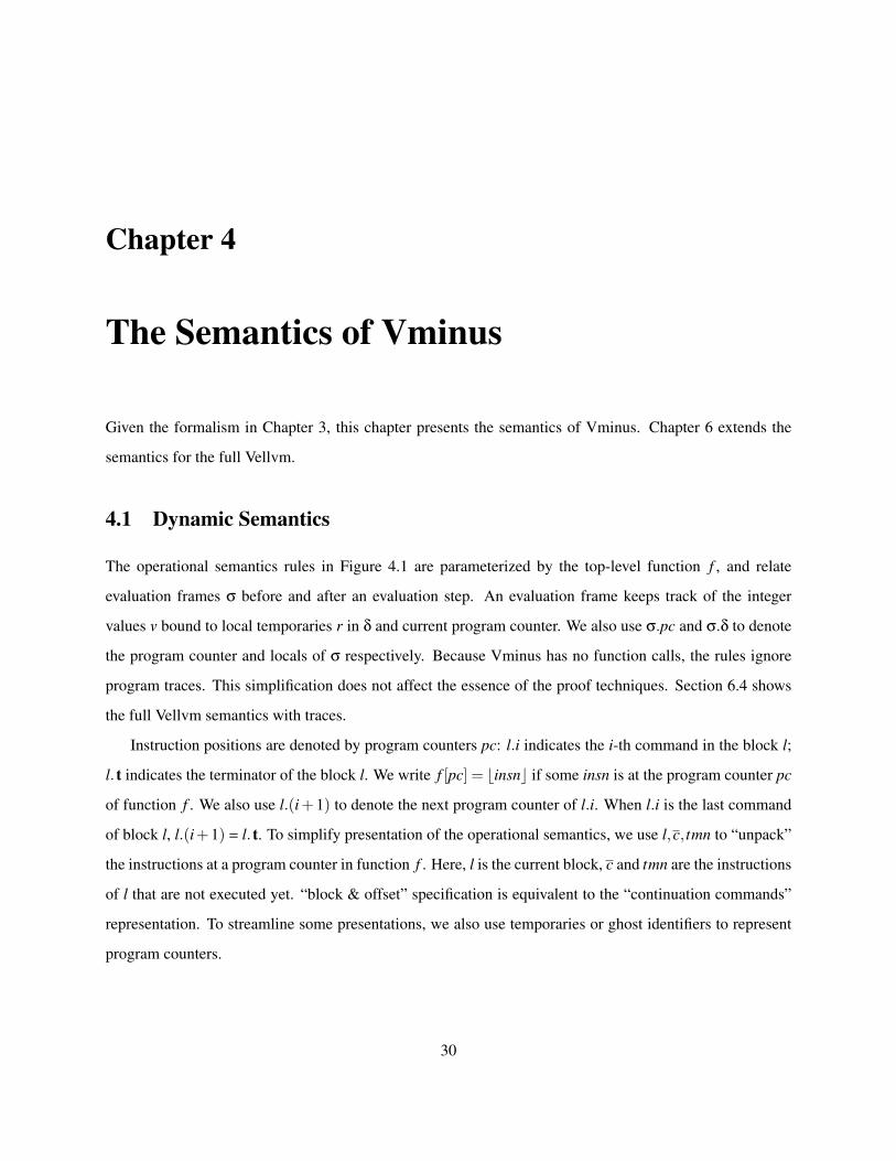
Chapter 4
The Semantics of Vminus
Given the formalism in Chapter 3, this chapter presents the semantics of Vminus. Chapter 6 extends the
semantics for the full Vellvm.
4.1 Dynamic Semantics
The operational semantics rules in Figure 4.1 are parameterized by the top-level function f , and relate
evaluation frames σ before and after an evaluation step. An evaluation frame keeps track of the integer
values v bound to local temporaries r in δ and current program counter. We also use σ.pc and σ.δ to denote
the program counter and locals of σ respectively. Because Vminus has no function calls, the rules ignore
program traces. This simplification does not affect the essence of the proof techniques. Section 6.4 shows
the full Vellvm semantics with traces.
Instruction positions are denoted by program counters pc: l.i indicates the i-th command in the block l;
l. t indicates the terminator of the block l. We write f [pc] = binsnc if some insn is at the program counter pc
of function f . We also use l.(i+1) to denote the next program counter of l.i. When l.i is the last command
of block l, l.(i+1) = l. t. To simplify presentation of the operational semantics, we use l,c, tmn to “unpack”
the instructions at a program counter in function f . Here, l is the current block, c and tmn are the instructions
of l that are not executed yet. “block & offset” specification is equivalent to the “continuation commands”
representation. To streamline some presentations, we also use temporaries or ghost identifiers to represent
program counters.
30
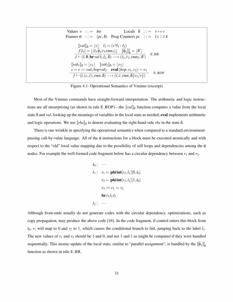
Values v : : = Int Locals δ : : = r 7→ vFrames σ : : = (pc,δ) Prog Counters pc : : = l.i | l. t
JvalKδ = bvc l3 = (v?l1 : l2)f [l3] = b(l3 φ3 c3 tmn3)c Jφ3Kl
δ= bδ′c
f ` (l, /0,brval l1 l2,δ)−→ (l3,c3, tmn3,δ′)E BR
Jval1Kδ = bv1c Jval2Kδ = bv2cc = r := val1 bopval2 eval(bop,v1,v2) = v3
f ` (l,(c,c), tmn,δ)−→ (l,c, tmn,δ{v3/r})E BOP
Figure 4.1: Operational Semantics of Vminus (excerpt)
Most of the Vminus commands have straight-forward interpretation. The arithmetic and logic instruc-
tions are all unsurprising (as shown in rule E BOP)—the JvalKδ function computes a value from the local
state δ and val, looking up the meanings of variables in the local state as needed; eval implements arithmetic
and logic operations. We use JrhsKδ to denote evaluating the right-hand-side rhs in the state δ.
There is one wrinkle in specifying the operational semantics when compared to a standard environment-
passing call-by-value language. All of the φ instructions for a block must be executed atomically and with
respect to the “old” local value mapping due to the possibility of self loops and dependencies among the φ
nodes. For example the well-formed code fragment below has a circular dependency between r1 and r2.
l0 : · · ·
l1 : r1 = phi int[r2, l1][0, l0]
r2 = phi int[r1, l1][1, l0]
r3 := r1 = r2
brr3 l1 l2
l2 : · · ·
Although front-ends usually do not generate codes with the circular dependency, optimizations, such as
copy propagation, may produce the above code [16]. In the code fragment, if control enters this block from
l0, r1 will map to 0 and r2 to 1, which causes the conditional branch to fail, jumping back to the label l1.
The new values of r1 and r2 should be 1 and 0, and not 1 and 1 as might be computed if they were handled
sequentially. This atomic update of the local state, similar to “parallel assignment”, is handled by the Jφ3Klδ
function as shown in rule E BR.
31
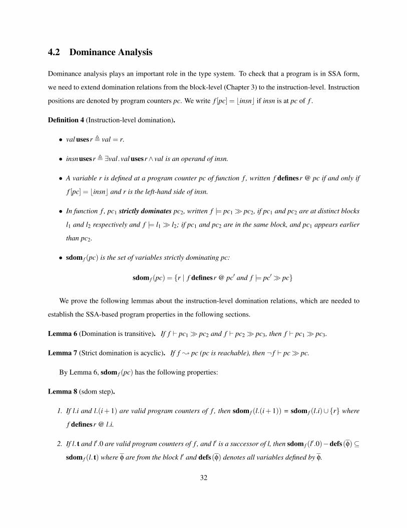
4.2 Dominance Analysis
Dominance analysis plays an important role in the type system. To check that a program is in SSA form,
we need to extend domination relations from the block-level (Chapter 3) to the instruction-level. Instruction
positions are denoted by program counters pc. We write f [pc] = binsnc if insn is at pc of f .
Definition 4 (Instruction-level domination).
• val usesr , val = r.
• insnusesr , ∃val.val usesr∧ val is an operand of insn.
• A variable r is defined at a program counter pc of function f , written f definesr @ pc if and only if
f [pc] = binsnc and r is the left-hand side of insn.
• In function f , pc1 strictly dominates pc2, written f |= pc1� pc2, if pc1 and pc2 are at distinct blocks
l1 and l2 respectively and f |= l1� l2; if pc1 and pc2 are in the same block, and pc1 appears earlier
than pc2.
• sdom f (pc) is the set of variables strictly dominating pc:
sdom f (pc) = {r | f definesr @ pc′ and f |= pc′� pc}
We prove the following lemmas about the instruction-level domination relations, which are needed to
establish the SSA-based program properties in the following sections.
Lemma 6 (Domination is transitive). If f ` pc1� pc2 and f ` pc2� pc3, then f ` pc1� pc3.
Lemma 7 (Strict domination is acyclic). If f ; pc (pc is reachable), then ¬ f ` pc� pc.
By Lemma 6, sdom f (pc) has the following properties:
Lemma 8 (sdom step).
1. If l.i and l.(i+ 1) are valid program counters of f , then sdom f (l.(i+ 1)) = sdom f (l.i)∪{r} where
f definesr @ l.i.
2. If l. t and l′.0 are valid program counters of f , and l′ is a successor of l, then sdom f (l′.0)−defs(φ)⊆
sdom f (l. t) where φ are from the block l′ and defs(φ) denotes all variables defined by φ.
32
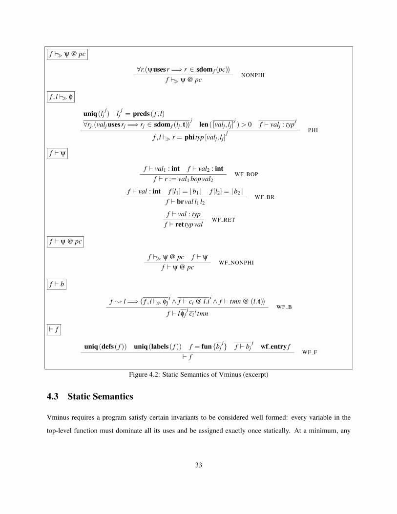
f � ψ @ pc
∀r.(ψusesr =⇒ r ∈ sdom f (pc))f � ψ @ pc
NONPHI
f , l � φ
uniq(ljj) lj
j= preds( f , l)
∀rj.(valj usesrj =⇒ rj ∈ sdom f (lj. t))j
len( [valj, lj]j)> 0 f ` valj : typ
j
f , l � r = phi typ [valj, lj]j PHI
f ` ψ
f ` val1 : int f ` val2 : intf ` r := val1 bopval2
WF BOP
f ` val : int f [l1] = bb1c f [l2] = bb2cf ` brval l1 l2
WF BR
f ` val : typf ` ret typval
WF RET
f ` ψ @ pc
f � ψ @ pc f ` ψ
f ` ψ @ pcWF NONPHI
f ` b
f ; l =⇒ ( f , l � φjj∧ f ` ci @ l.i
i∧ f ` tmn @ (l. t))
f ` lφjj ci
i tmnWF B
` f
uniq(defs( f )) uniq(labels( f )) f = fun{bjj} f ` bj
j wf entry f` f
WF F
Figure 4.2: Static Semantics of Vminus (excerpt)
4.3 Static Semantics
Vminus requires a program satisfy certain invariants to be considered well formed: every variable in the
top-level function must dominate all its uses and be assigned exactly once statically. At a minimum, any
33
reasonable Vminus transformation must preserve these invariants; together they imply that the program is
in SSA form [28].
Figure 4.2 shows the judgments to check the SSA invariants with respect to the control-flow graph and
program points of the function f .
Rule WF F ensures that variables defs( f ) defined in the top function must be unique, which enforces
the single-assignment part of the SSA property; additionally all block labels labels( f ) in the function must
also be unique for a well-formed control-flow graph; the entry block has no predecessors (wf entry f ).
Rule WF B checks that all instructions in reachable blocks (written f ; l) satisfy the SSA domination
invariant. Because unreachable blocks have no effects at runtime, the rule does not check them. Rule
NONPHI ensures that a ψ at pc must be strictly dominated by the definitions of all variables used by ψ; the
rule PHI ensures that the number of incoming values is not zero, that all incoming labels are unique, and that
the current block’s predecessors is the same as the set of incoming gables. If an incoming value valj from a
predecessor block lj uses a variable rj at pcj, then pcj must strictly dominate the terminator of lj. Importantly,
this rule allows “cyclic” uses of SSA variables of the kind used in the example above (Section 4.1).
Given the semantics in this chapter, the next chapter presents the proof techniques for reasoning about
SSA-based program properties and transformations of Vminus.
34
Chapter 5
Proof Techniques for SSA
This section describes the proof techniques we have developed for formalizing properties of SSA-style
intermediate representations. To most clearly articulate the approach, we present the results using Vminus
(see Chapter 4).
The key idea of the technique is to generalize the invariant used for Vminus’s preservation lemma for
proving safety to other predicates that are also shown to be invariants of the operational semantics. Crucially,
these predicates all share the same form, which only constrains variable definitions that strictly dominate
the current program counter. Because Vminus is such a stripped-down language, the relevant lemmas are
relatively straightforward to establish; Chapter 8 shows how to scale the proof technique to the full Vellvm
model of LLVM to verify the mem2reg pass.
Instances of this idea are found in the literature (see, for example, Menon, et al. [48]), and related proof
techniques have been recently used in the CompCertSSA [14] project, but as we explain in Chapter 10, our
results are more general: we provide proof techniques applicable to many SSA-based optimizations and
transformations.
The remainder of this section first proves safety (which in this context simply amounts to showing
that all variables are well-scoped). We then show how to generalize the safety invariant to a form that is
useful for proving program transformations correct and demonstrate its applicability to a number of standard
optimizations.
We mechanically verified all the claims in this chapter for Vminus in Coq.1
1Annotated Coq source available at http://www.cis.upenn.edu/~stevez/vellvm/.
35
5.1 Safety of Vminus
There are two ways that a Vminus program might get stuck. First, it might try to jump to an undefined label,
but this property is ruled out statically by WF BR. Second, it might try to access a variable whose value
is not defined in δ. We can prove that this second case never happens by establishing the following safety
theorem:
Theorem 9 (Safety). If ` f and f ` (l.0, /0)−→∗ σ, then σ is not stuck. (Here, l is the entry block of function
f and /0 denotes an empty mapping for identifiers.)
The proof takes the standard form using preservation and progress lemmas with the invariant for frames
shown below:pc ∈ f ∀r.(r ∈ sdom f (pc) =⇒∃v.δ[r] = bvc)
f ` (pc,δ)WF FR
This is similar to the predicate used in prior work for verifying the type safety of an SSA-based lan-
guage [48]. The invariant WF FR shows that a frame (pc,δ) is well-formed if every definition that strictly
dominates pc is defined in δ. The initial program state satisfies this invariant trivially:
Lemma 10 (Initial State). If ` f then f ` (l.0, /0), where l is the entry block of f .
The preservation and progress lemmas are straightforward—but note that they crucially rely on the
interplay between the invariant on δ “projected” onto sdom f (pc) (Lemma 8), and the PHI and NONPHI
rules of the static semantics.
Lemma 11 (Preservation). If ` f , f ` σ and f ` σ−→ σ′, then f ` σ′.
Proof. The proof proceeds by case analysis on the reduction rule. At the E BOP case: Let σ = (l.i,δ), σ′ =
(l.(i+1),δ{v3/r}), and f [l.i] = br := val1 bopval2c. The conclusion holds by Lemma 8.
At the E BR case: Let σ = (l. t,δ), σ′ = (l3.0,δ′), f [l. t] = bbrval l1 l2c, Jφ3Klδ= bδ′c, and φ3 is from the
block l3. Suppose r ∈ sdom f (l3.0). If r ∈ defs(φ3), then r must be defined in δ′ by the definition of TUlφ3
.
Otherwise, if ¬r ∈ defs(φ3), the conclusion holds by Lemma 8.
Lemma 12 (Progress). If ` f , f ` σ, then σ is not stuck.
36

Proof. Assume that σ = (pc,δ). Since pc ∈ f , then ∃insn. f [pc] = binsnc. The proof proceeds by case
analysis on the insn. At the case when insn = r := val1 bopval2: The rule NONPHI ensures that the
definitions of the variables used by val1 and val2 strictly dominate pc, so are in sdom f (pc). Therefore, σ is
not stuck.
At the case when insn = brval l1 l2: First, the rule NONPHI ensures that the val must use the variable
defined in sdom f (pc). Therefore, JvalKδ = bvc. Suppose l3 = (v?l1 : l2), f [l3] = b(l3 φ3 c3 tmn3)c, and insn
is at block lj. The rule PHI ensures that the definitions of the j-th incoming variables dominate lj. t, so are
in sdom f (pc). Therefore, Jφ3Klδ= bδ′c.
At the case when insn = ret typval: The program terminates.
5.2 Generalizing Safety to Other SSA Invariants
The main feature of the preservation proof, Lemma 11, is that the constraint on sdom f (pc) is an invariant
of the operational semantics. But—and this is a key observation—we can parameterize rule WF FR by a
predicate P, which is an arbitrary proposition about functions and frames:
σ.pc ∈ f P f (σ| f )
f ,P ` σ
GWF FR
Here, σ| f is (σ.pc,(σ.δ)|(sdom f (σ.pc))) and we write (δ|R)[r] = bvc iff r ∈ R and δ[r] = bvc and observe that
dom(δ|R) = R. These restrictions say that we don’t need to consider all variables: Intuitively, because SSA
invariants are based on dominance properties, when reasoning about a program state we need consider only
the variable definitions that strictly dominate the program counter in a given state.
For proving Theorem 9, we instantiated P to be:
Psafety , λ f .λσ.∀r.r ∈ dom(σ.δ) =⇒∃v.(σ.δ)[r] = bvc
For safety, it is enough to show that each variable in the domination set is well defined at its use. To
prove program transformations correct, we instantiate P with a different predicate, Psem, that relates the
syntactic definition of a variable with the semantic value:
λ f .λσ.∀r. f [r] = brhsc=⇒ (σ.δ)[r] 6= none =⇒ (σ.δ)[r] = JrhsK(σ.δ)
This predicate ensures that if a definition r is in scope, the value of r must equal to the value to which the
right-hand-side of its definition evaluates.
37
Just as we proved preservation for Psafety, we can also prove preservation for Psem (using Lemma 4):
Theorem 13. If ` f and f ,Psem ` σ and f ` σ−→ σ′, then f ,Psem ` σ′.
Proof (sketch): Suppose a command r := rhs is defined at a program counter pc1. The NONPHI rule
ensures that all variables used by rhs must strictly dominate pc1. Because strict domination relation is
acyclic (Lemma 4), at any program counter pc2 that pc1 strictly dominates, the program cannot define r and
any variable used by rhs. In other words, the values of r and rhs are not changed between pc1 and pc2. The
result follows immediately.
Theorem 13 shows the dynamic property of an SSA variable: the value of r is invariant in any execution
path that its definition strictly dominates. As we show next, Theorem 13 can be used to justify the correctness
of many SSA-based transformations. Instantiating P with other predicates can also be useful—Section 8.3
shows how.
5.3 The Correctness of SSA-based Transformations
Consider again the example code transformation from Figure 2.2. It, and many other SSA-based optimiza-
tions, can be defined by using a combination of simpler transformations: deleting an unused definition,
substituting a constant expression for a variable, substituting one variable by another, or moving variable
definitions. Each such transformation is subject to the SSA constraints—for example, we can’t move a
definition later than one of its uses—and each transformation preserves the SSA invariants. By pipelining
these basic transformations, we can define more sophisticated SSA-based program transformations whose
correctness is established by the composition of the proofs for the basic transformations.
In general, an SSA-based transformation from f to f ′ is correct if it preserves both well-formedness and
program behavior.
1. Preserving well-formedness: if ` f , then ` f ′.
2. Program refinement: if ` f , then f ⊇ f ′.
Here, behaviors of a Vminus program include whether the program terminates, and the returned value if it
does (see Section 2.1).
Each of the basic transformations mentioned above can be proved correct by using Theorem 13. Here
we present only the correctness of variable substitution (although we proved correct all the mentioned
38
transformations in our Coq development). Chapter 8 shows how to extend the transformations to implement
memory-aware optimizations in the full Vellvm.
Variable substitution Consider the step of the program transformation from Figure 2.2 in which the use
of r8 on the last line is replaced by r4 (this is valid only after hoisting the definition of r4 so that it is in
scope). This transformation is correct because both r4 and r8 denote the same value, and the definition
of r4 (after hoisting) strictly dominates the definition of r8. In Figure 2.2, it is enough to do redundant
variable elimination—this optimization lets us replace one variable by another when their definitions are
syntactically equal; other optimizations, such as global value numbering, allow a coarser, more semantic,
equality to be used. Proving them correct follows the same basic pattern as the proof shown below.
Definition 5 (Redundant Variable). In a function f , a variable r2 is redundant with variable r1 if:
1. f definesr1 @ pc1, f definesr2 @ pc2 and f |= pc1� pc2
2. f [pc1] = bc1c, f [pc1] = bc2c and c1 and c2 have syntactically equal right-hand-sides.
We would like to prove that eliminating a redundant variable is correct, and therefore must relate a
program f with f{r1/r2}, in which all uses of r2 have been substituted by r1.
Since substitution does not change the control-flow graph, it preserves the domination relations.
Lemma 14.
1. f |= l1�= l2 ⇐⇒ f{r2/r1} |= l1�= l2
2. f |= pc1� pc2 ⇐⇒ f{r2/r1} |= pc1� pc2
Applying Lemma 2 and Lemma 14, we have:
Lemma 15 ( f{r2/r1} preserves well-formedness). Suppose that in f , r1 is redundant with r2. If ` f , then
` f{r2/r1}.
Let two program states simulate each other if they have the same local state δ and program counter. We
assume that the original program and its transformation have the same initial state.
Lemma 16. If ` f , r2 is redundant with r1 in f , and (pc,δ) is a reachable state, then
39
1. If val is an operand of a non-phinode at program counter pc, then ∃v.JvalKδ = bvc∧ Jval{r1/r2}Kδ =
bvc.
2. If pc is li. t, and li is a previous block of a block with φ-nodes φjj, then ∃δ′.Jφj
jKliδ= bδ′c ∧
Jφj{r1/r2}jKli
δ= bδ′c.
Proof (sketch): The proof makes crucial use of Theorem 13. For example, to show part 1 for a source
instruction r := rhs (with transformed instruction r := rhs{r1/r2}) located at program counter pc, we reason
like this: if r2 is an operand used by rhs, then r2 ∈ sdom f (pc) and by Theorem 13, property Psem, implies
that δ[r2] = Jrhs2Kδ for some rhs2 defining r2. Since r1 is used as an operand in rhs{r1/r2}, similar reasoning
shows that δ[r1] = Jrhs1Kδ, but since r2 is redundant with r1, we have rhs2 = rhs1, and the result follows
immediately.
Using Lemma 16, we can easily show the lock-step simulation lemma, which completes the correctness
proof:
Lemma 17. If ` f , r2 is redundant with r1 in f , f{r1/r2} ` σ1 −→ σ2, then f ` σ1 −→ σ2.
This chapter showed the proof techniques for reasoning about SSA-based program properties and trans-
formations of Vminus. To demonstrate that our proof techniques can be used for practical compiler opti-
mizations, the following chapters present how to verify program transformations of the full LLVM IR.
40
Chapter 6
The formalism of the LLVM IR
Vminus provides a convenient minimal setting in which to study SSA-based optimizations, but it omits
many features necessary in a real intermediate representation. To demonstrate that our proof techniques can
be used for practical compiler optimizations, we next show how to apply them to the LLVM IR.
The Vellvm infrastructure provides a Coq implementation of the full LLVM intermediate language
and defines (several) operational semantics along with some useful metatheory about the memory model.
Vellvm’s formalization is based on the LLVM release version 3.0, and the syntax and semantics are intended
to model the behavior as described in the LLVM Language Reference 1, although we also used the LLVM
IR reference interpreter and the x86 backend to inform our design. The chapter describes the syntax and
semantics of the LLVM IR, emphasizing those features that are either unique to the LLVM or have non-
trivial implications for the formalization.
6.1 The Syntax
Figure 6.1 and Figure 6.2 show the abstract syntax for the subset of the LLVM IR formalized in Vellvm.
The metavariable id ranges over LLVM identifiers, written %X, %T, %a, %b, etc., which are used to name local
types and temporary variables, and @a, @b, @main, etc., which name global values and functions.
Each source file is a module mod (which is also called a program P) that includes data layout information
layout (which defines sizes and alignments for types; see below), named types, and a list of prods that can
1See http://llvm.org/releases/3.0/docs/LangRef.html
41
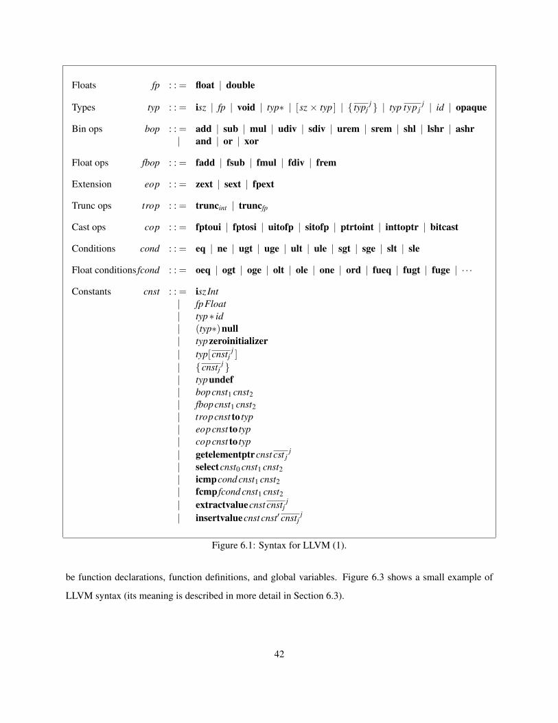
Floats fp : : = float | double
Types typ : : = isz | fp | void | typ∗ | [sz × typ ] | { typjj } | typ typ j
j | id | opaque
Bin ops bop : : = add | sub | mul | udiv | sdiv | urem | srem | shl | lshr | ashr| and | or | xor
Float ops fbop : : = fadd | fsub | fmul | fdiv | frem
Extension eop : : = zext | sext | fpext
Trunc ops trop : : = truncint | truncfp
Cast ops cop : : = fptoui | fptosi | uitofp | sitofp | ptrtoint | inttoptr | bitcast
Conditions cond : : = eq | ne | ugt | uge | ult | ule | sgt | sge | slt | sle
Float conditions fcond : : = oeq | ogt | oge | olt | ole | one | ord | fueq | fugt | fuge | · · ·
Constants cnst : : = isz Int| fpFloat| typ∗ id| (typ∗)null| typzeroinitializer| typ[cnstj
j ]
| {cnstjj }
| typundef| bopcnst1 cnst2| fbopcnst1 cnst2| tropcnst to typ| eopcnst to typ| copcnst to typ| getelementptrcnst cst j
j
| selectcnst0 cnst1 cnst2| icmpcond cnst1 cnst2| fcmp fcond cnst1 cnst2
| extractvaluecnst cnstjj
| insertvaluecnst cnst′ cnstjj
Figure 6.1: Syntax for LLVM (1).
be function declarations, function definitions, and global variables. Figure 6.3 shows a small example of
LLVM syntax (its meaning is described in more detail in Section 6.3).
42

Modules mod,P : : = layout namedt prod
Layouts layout : : = bigendian | littleendian | ptrszalign0 align1 | intszalign0 align1| floatszalign0 align1 | aggrszalign0 align1 | stackszalign0 align1
Products prod : : = id = global typconst align | define typ id(arg){b} | declare typ id(arg)
Values val : : = id | cnst
Blocks b : : = lφctmn
φ nodes φ : : = id = phi typ [valj, lj]j
Tmns tmn : : = brval l1 l2| br l| ret typval| retvoid| unreachable
Commands c : : = id = bop( intsz)val1 val2| id = fbopfpval1 val2| store typval1 val2 align| id = load(typ∗)val1 align| id = malloc typval align| free( typ∗)val| id = alloca typval align| id = trop typ1 val to typ2| id = eoptyp1 val to typ2| id = coptyp1 val to typ2| id = icmpcond typval1 val2| id = selectval0 typval1 val2| id = fcmp fcond fpval1 val2| option id = call typ0 val0 param| id = getelementptr( typ∗)val val j
j
| id = extractvalue typval cnstjj
| id = insertvalue typval typ′ val′ cnstjj
Figure 6.2: Syntax for LLVM (2).
Every LLVM expression has a type, which can easily be determined from type annotations that provide
sufficient information to check an LLVM program for type compatibility. The LLVM IR is not a type-safe
language, however, because its type system allows arbitrary casts, calling functions with incorrect signatures,
accessing invalid memory, etc. The LLVM type system ensures only that the size of a runtime value in a
43

%ST = type { i10 , [10 x i8*] }
define %ST* @foo(i8* %ptr) {
entry:
%p = malloc %ST, i32 1
%r = getelementptr %ST* %p, i32 0, i32 0
store i10 648, %r ; decomposes as 136, 2
%s = getelementptr %ST* %p, i32 0, i32 1, i32 0
store i8* %ptr, %s
ret %ST* %p
}
Here, %p is a pointer to a single-element array of structures of type %ST. Pointer %r indexes into the firstcomponent of the first element in the array, and has type i10*, as used by the subsequent store, which writesthe 10-bit value 648. Pointer %s has type i8** and points to the first element of the nested array in the samestructure.
Figure 6.3: An example use of LLVM’s memory operations.
well-formed program is compatible with the type of the value—a well-formed program can still be stuck
(see Section 6.4.3).
Types typ include arbitrary bit-width integers i8, i16, i32, etc., or, more generally, isz where sz is a
natural number. Types also include float, void, pointers typ∗, arrays [sz × typ ] that have a statically-known
size sz. Anonymous structure types { typjj } contain a list of types. Functions typ typ j
j have a return type,
and a list of argument types. Here, typjj denotes a list of typ components; we use similar notation for other
lists throughout the paper. Finally, types can be named by identifiers id which is useful to define recursive
types.
The sizes and alignments for types, and endianness are defined in layout. For example.
intszalign0 align1 dictates that values with type isz are align0-byte aligned when they are within an
aggregate and when used as an argument, and align1-byte aligned when emitted as a global.
Operations in the LLVM IR compute with values val, which are either identifiers id naming temporaries,
or constants cnst computed from statically-known data, using the compile-time analogs of the commands
described below. Constants include base values (i.e., integers or floats of a given bit width), and zero-values
of a given type, as well as structures and arrays built from other constants.
To account for uninitialized variables and to allow for various program optimizations, the LLVM IR
also supports a type-indexed undef constant. Semantically, undef stands for a set of possible bit patterns,
and LLVM compilers are free to pick convenient values for each occurrence of undef to enable aggressive
44
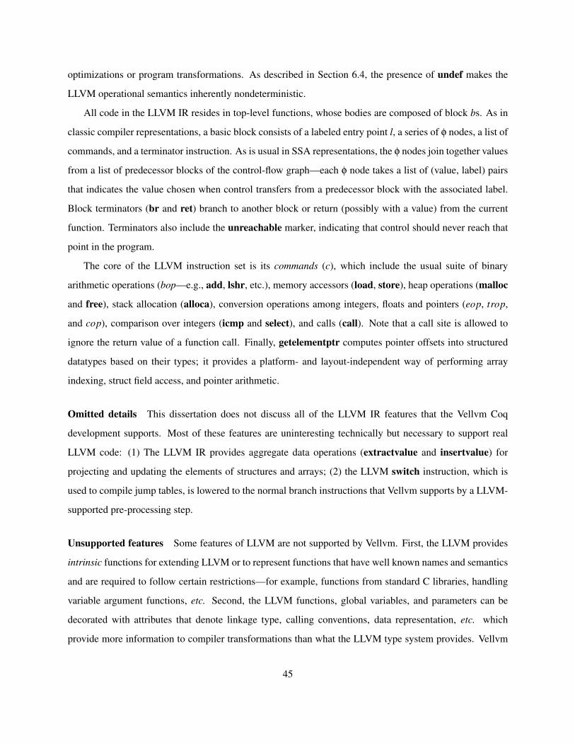
optimizations or program transformations. As described in Section 6.4, the presence of undef makes the
LLVM operational semantics inherently nondeterministic.
All code in the LLVM IR resides in top-level functions, whose bodies are composed of block bs. As in
classic compiler representations, a basic block consists of a labeled entry point l, a series of φ nodes, a list of
commands, and a terminator instruction. As is usual in SSA representations, the φ nodes join together values
from a list of predecessor blocks of the control-flow graph—each φ node takes a list of (value, label) pairs
that indicates the value chosen when control transfers from a predecessor block with the associated label.
Block terminators (br and ret) branch to another block or return (possibly with a value) from the current
function. Terminators also include the unreachable marker, indicating that control should never reach that
point in the program.
The core of the LLVM instruction set is its commands (c), which include the usual suite of binary
arithmetic operations (bop—e.g., add, lshr, etc.), memory accessors (load, store), heap operations (malloc
and free), stack allocation (alloca), conversion operations among integers, floats and pointers (eop, trop,
and cop), comparison over integers (icmp and select), and calls (call). Note that a call site is allowed to
ignore the return value of a function call. Finally, getelementptr computes pointer offsets into structured
datatypes based on their types; it provides a platform- and layout-independent way of performing array
indexing, struct field access, and pointer arithmetic.
Omitted details This dissertation does not discuss all of the LLVM IR features that the Vellvm Coq
development supports. Most of these features are uninteresting technically but necessary to support real
LLVM code: (1) The LLVM IR provides aggregate data operations (extractvalue and insertvalue) for
projecting and updating the elements of structures and arrays; (2) the LLVM switch instruction, which is
used to compile jump tables, is lowered to the normal branch instructions that Vellvm supports by a LLVM-
supported pre-processing step.
Unsupported features Some features of LLVM are not supported by Vellvm. First, the LLVM provides
intrinsic functions for extending LLVM or to represent functions that have well known names and semantics
and are required to follow certain restrictions—for example, functions from standard C libraries, handling
variable argument functions, etc. Second, the LLVM functions, global variables, and parameters can be
decorated with attributes that denote linkage type, calling conventions, data representation, etc. which
provide more information to compiler transformations than what the LLVM type system provides. Vellvm
45
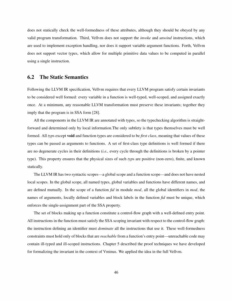
does not statically check the well-formedness of these attributes, although they should be obeyed by any
valid program transformation. Third, Vellvm does not support the invoke and unwind instructions, which
are used to implement exception handling, nor does it support variable argument functions. Forth, Vellvm
does not support vector types, which allow for multiple primitive data values to be computed in parallel
using a single instruction.
6.2 The Static Semantics
Following the LLVM IR specification, Vellvm requires that every LLVM program satisfy certain invariants
to be considered well formed: every variable in a function is well-typed, well-scoped, and assigned exactly
once. At a minimum, any reasonable LLVM transformation must preserve these invariants; together they
imply that the program is in SSA form [28].
All the components in the LLVM IR are annotated with types, so the typechecking algorithm is straight-
forward and determined only by local information.The only subtlety is that types themselves must be well
formed. All typs except void and function types are considered to be first class, meaning that values of these
types can be passed as arguments to functions. A set of first-class type definitions is well formed if there
are no degenerate cycles in their definitions (i.e., every cycle through the definitions is broken by a pointer
type). This property ensures that the physical sizes of such typs are positive (non-zero), finite, and known
statically.
The LLVM IR has two syntactic scopes—a global scope and a function scope—and does not have nested
local scopes. In the global scope, all named types, global variables and functions have different names, and
are defined mutually. In the scope of a function fid in module mod, all the global identifiers in mod, the
names of arguments, locally defined variables and block labels in the function fid must be unique, which
enforces the single-assignment part of the SSA property.
The set of blocks making up a function constitute a control-flow graph with a well-defined entry point.
All instructions in the function must satisfy the SSA scoping invariant with respect to the control-flow graph:
the instruction defining an identifier must dominate all the instructions that use it. These well-formedness
constraints must hold only of blocks that are reachable from a function’s entry point—unreachable code may
contain ill-typed and ill-scoped instructions. Chapter 5 described the proof techniques we have developed
for formalizing the invariant in the context of Vminus. We applied the idea in the full Vellvm.
46
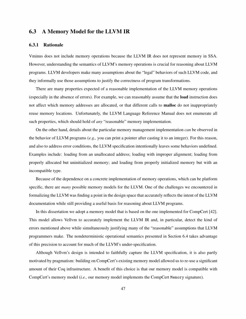
6.3 A Memory Model for the LLVM IR
6.3.1 Rationale
Vminus does not include memory operations because the LLVM IR does not represent memory in SSA.
However, understanding the semantics of LLVM’s memory operations is crucial for reasoning about LLVM
programs. LLVM developers make many assumptions about the “legal” behaviors of such LLVM code, and
they informally use those assumptions to justify the correctness of program transformations.
There are many properties expected of a reasonable implementation of the LLVM memory operations
(especially in the absence of errors). For example, we can reasonably assume that the load instruction does
not affect which memory addresses are allocated, or that different calls to malloc do not inappropriately
reuse memory locations. Unfortunately, the LLVM Language Reference Manual does not enumerate all
such properties, which should hold of any “reasonable” memory implementation.
On the other hand, details about the particular memory management implementation can be observed in
the behavior of LLVM programs (e.g., you can print a pointer after casting it to an integer). For this reason,
and also to address error conditions, the LLVM specification intentionally leaves some behaviors undefined.
Examples include: loading from an unallocated address; loading with improper alignment; loading from
properly allocated but uninitialized memory; and loading from properly initialized memory but with an
incompatible type.
Because of the dependence on a concrete implementation of memory operations, which can be platform
specific, there are many possible memory models for the LLVM. One of the challenges we encountered in
formalizing the LLVM was finding a point in the design space that accurately reflects the intent of the LLVM
documentation while still providing a useful basis for reasoning about LLVM programs.
In this dissertation we adopt a memory model that is based on the one implemented for CompCert [42].
This model allows Vellvm to accurately implement the LLVM IR and, in particular, detect the kind of
errors mentioned above while simultaneously justifying many of the “reasonable” assumptions that LLVM
programmers make. The nondeterministic operational semantics presented in Section 6.4 takes advantage
of this precision to account for much of the LLVM’s under-specification.
Although Vellvm’s design is intended to faithfully capture the LLVM specification, it is also partly
motivated by pragmatism: building on CompCert’s existing memory model allowed us to re-use a significant
amount of their Coq infrastructure. A benefit of this choice is that our memory model is compatible with
CompCert’s memory model (i.e., our memory model implements the CompCert Memory signature).
47
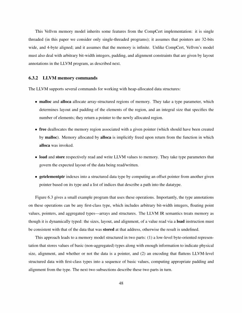
This Vellvm memory model inherits some features from the CompCert implementation: it is single
threaded (in this paper we consider only single-threaded programs); it assumes that pointers are 32-bits
wide, and 4-byte aligned; and it assumes that the memory is infinite. Unlike CompCert, Vellvm’s model
must also deal with arbitrary bit-width integers, padding, and alignment constraints that are given by layout
annotations in the LLVM program, as described next.
6.3.2 LLVM memory commands
The LLVM supports several commands for working with heap-allocated data structures:
• malloc and alloca allocate array-structured regions of memory. They take a type parameter, which
determines layout and padding of the elements of the region, and an integral size that specifies the
number of elements; they return a pointer to the newly allocated region.
• free deallocates the memory region associated with a given pointer (which should have been created
by malloc). Memory allocated by alloca is implicitly freed upon return from the function in which
alloca was invoked.
• load and store respectively read and write LLVM values to memory. They take type parameters that
govern the expected layout of the data being read/written.
• getelementptr indexes into a structured data type by computing an offset pointer from another given
pointer based on its type and a list of indices that describe a path into the datatype.
Figure 6.3 gives a small example program that uses these operations. Importantly, the type annotations
on these operations can be any first-class type, which includes arbitrary bit-width integers, floating point
values, pointers, and aggregated types—arrays and structures. The LLVM IR semantics treats memory as
though it is dynamically typed: the sizes, layout, and alignment, of a value read via a load instruction must
be consistent with that of the data that was stored at that address, otherwise the result is undefined.
This approach leads to a memory model structured in two parts: (1) a low-level byte-oriented represen-
tation that stores values of basic (non-aggregated) types along with enough information to indicate physical
size, alignment, and whether or not the data is a pointer, and (2) an encoding that flattens LLVM-level
structured data with first-class types into a sequence of basic values, computing appropriate padding and
alignment from the type. The next two subsections describe these two parts in turn.
48
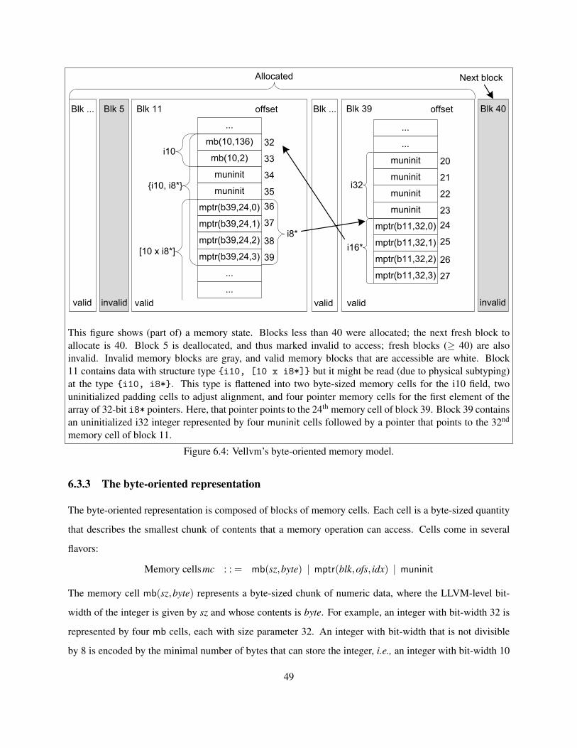
Blk ... Blk 39Blk 11
mb(10,2)
muninit
mptr(b39,24,0)
mptr(b39,24,1)
mptr(b39,24,2)
mptr(b39,24,3)
muninit
mb(10,136)i10
muninit
mptr(b11,32,0)
mptr(b11,32,1)
mptr(b11,32,2)
mptr(b11,32,3)
muninit
i32
i16*
muninit
muninit{i10, i8*}
32
33
34
35
36
37
38
39
offset
20
21
22
23
24
25
26
27
offset
...
...
...
...
...
Blk 40
Allocated
Blk 5Blk ...
valid valid validinvalid invalidvalid
Next block
i8*
[10 x i8*]
This figure shows (part of) a memory state. Blocks less than 40 were allocated; the next fresh block toallocate is 40. Block 5 is deallocated, and thus marked invalid to access; fresh blocks (≥ 40) are alsoinvalid. Invalid memory blocks are gray, and valid memory blocks that are accessible are white. Block11 contains data with structure type {i10, [10 x i8*]} but it might be read (due to physical subtyping)at the type {i10, i8*}. This type is flattened into two byte-sized memory cells for the i10 field, twouninitialized padding cells to adjust alignment, and four pointer memory cells for the first element of thearray of 32-bit i8* pointers. Here, that pointer points to the 24th memory cell of block 39. Block 39 containsan uninitialized i32 integer represented by four muninit cells followed by a pointer that points to the 32nd
memory cell of block 11.
Figure 6.4: Vellvm’s byte-oriented memory model.
6.3.3 The byte-oriented representation
The byte-oriented representation is composed of blocks of memory cells. Each cell is a byte-sized quantity
that describes the smallest chunk of contents that a memory operation can access. Cells come in several
flavors:
Memory cellsmc : : = mb(sz,byte) | mptr(blk,ofs, idx) | muninit
The memory cell mb(sz,byte) represents a byte-sized chunk of numeric data, where the LLVM-level bit-
width of the integer is given by sz and whose contents is byte. For example, an integer with bit-width 32 is
represented by four mb cells, each with size parameter 32. An integer with bit-width that is not divisible
by 8 is encoded by the minimal number of bytes that can store the integer, i.e., an integer with bit-width 10
49
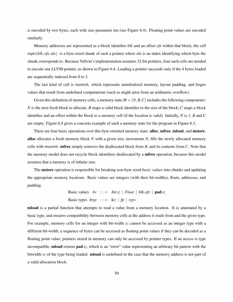
is encoded by two bytes, each with size parameter ten (see Figure 6.4). Floating point values are encoded
similarly.
Memory addresses are represented as a block identifier blk and an offset ofs within that block; the cell
mptr(blk,ofs, idx) is a byte-sized chunk of such a pointer where idx is an index identifying which byte the
chunk corresponds to. Because Vellvm’s implementation assumes 32-bit pointers, four such cells are needed
to encode one LLVM-pointer, as shown in Figure 6.4. Loading a pointer succeeds only if the 4 bytes loaded
are sequentially indexed from 0 to 3.
The last kind of cell is muninit, which represents uninitialized memory, layout padding, and bogus
values that result from undefined computations (such as might arise from an arithmetic overflow).
Given this definition of memory cells, a memory state M = (N,B,C) includes the following components:
N is the next fresh block to allocate, B maps a valid block identifier to the size of the block; C maps a block
identifier and an offset within the block to a memory cell (if the location is valid). Initially, N is 1; B and C
are empty. Figure 6.4 gives a concrete example of such a memory state for the program in Figure 6.3.
There are four basic operations over this byte-oriented memory state: alloc, mfree, mload, and mstore.
alloc allocates a fresh memory block N with a given size, increments N, fills the newly allocated memory
cells with muninit. mfree simply removes the deallocated block from B, and its contents from C. Note that
the memory model does not recycle block identifiers deallocated by a mfree operation, because this model
assumes that a memory is of infinite size.
The mstore operation is responsible for breaking non-byte sized basic values into chunks and updating
the appropriate memory locations. Basic values are integers (with their bit-widths), floats, addresses, and
padding.
Basic values bv : : = Int sz | Float | blk.ofs | padsz
Basic types btyp : : = isz | fp | typ∗
mload is a partial function that attempts to read a value from a memory location. It is annotated by a
basic type, and ensures compatibility between memory cells at the address it reads from and the given type.
For example, memory cells for an integer with bit-width sz cannot be accessed as an integer type with a
different bit-width; a sequence of bytes can be accessed as floating point values if they can be decoded as a
floating point value; pointers stored in memory can only be accessed by pointer types. If an access is type
incompatible, mload returns padsz, which is an “error” value representing an arbitrary bit pattern with the
bitwidth sz of the type being loaded. mload is undefined in the case that the memory address is not part of
a valid allocation block.
50

6.3.4 The LLVM flattened values and memory accesses
LLVM’s structured data is flattened to lists of basic values that indicate its physical representation:
Flattened Valuesv : : = bv | bv,v
A constant cnst is flattened into a list of basic values according to it annotated type. If the cnst is already of
basic type, it flattens into the singleton list. Values of array type [sz × typ ] are first flattened element-wise
according to the representation given by typ and then padded by uninitialized values to match typ’s alignment
requirements as determined by the module’s layout descriptor. The resulting list is then concatenated to
obtain the appropriate flattened value. The case when a cnst is a structure type is similar.
The LLVM load instruction works by first flattening its type annotation typ into a list of basic types, and
mapping mload across the list; it then merges the returned basic values into the final LLVM value. Storing
an LLVM value to memory works by first flattening to a list of basic values and mapping mstore over the
result.
This scheme induces a notion of dynamically-checked physical subtyping: it is permitted to read a
structured value at a different type from the one at which it was written, so long as the basic types they
flatten into agree. For non-structured data types such as integers, Vellvm’s implementation is conservative—
for example, reading an integer with bit width two from the second byte of a 10-bit wide integer yields
undef because the results are, in general, platform specific. Because of this dynamically-checked, physical
subtyping, pointer-to-pointer casts can be treated as the identity. Similar ideas arise in other formalizations
of low-level language semantics [54, 55].
The LLVM malloc and free operations are defined by alloc and mfree in a straightforward manner.
As the LLVM IR does not explicitly distinguish the heap and stack and function calls are implementation-
specific, the memory model defines the same semantics for stack allocation (alloca) and heap allocation
(malloc) — both of them allocate memory blocks in memory. However, the operational semantics (described
next) maintains a list of blocks allocated by alloca for each function, and it deallocates them on return.
6.4 Operational Semantics
Vellvm provides several related operational semantics for the LLVM IR, as summarized in Figure 6.5. The
most general is LLVMND, a small-step, nondeterministic evaluation relation given by rules of the form
config ` S� S′ (see Figure 6.6). This section first motivates the need for nondeterminism in understanding
51

LLVMND
∈
LLVMInterp ≈ LLVMD & LLVM∗DFn & LLVM∗DB
Figure 6.5: Relations between different operational semantics, which are justified by proofs in Vellvm.
the LLVM semantics and then illustrates LLVMND by explaining some of its rules. Next, we introduce sev-
eral equivalent deterministic refinements of LLVMND—LLVMD, LLVM∗DB, and LLVM∗DFn—each of which
has different uses, as described in Section 6.4.4. All of these operational semantics must handle various
error conditions, which manifest as partiality in the rules. Section 6.4.3 describes these error conditions, and
relates them to the static semantics of Section 6.2.
Vellvm’s operational rules are specified as transitions between machine states S of the form M,Σ, where
M is the memory and Σ is a stack of frames. A frame keeps track of the current function fid and block label
l, as well as the “continuation” sequence of commands c to execute next ending with the block terminator
tmn. The map ∆ tracks bindings for the local variables (which are not stored in M), and the list α keeps track
of which memory blocks were created by the alloca instruction so that they can be marked as invalid when
the function call returns.
Value sets V : : = {v |Φ(v)} Locals ∆ : : = id 7→ V
Allocas α : : = [] | blk,α Frames Σ : : = fid, l,c, tmn,∆,α
Call stacks Σ : : = [] | Σ,Σ Program states S : : = M,Σ
6.4.1 Nondeterminism in the LLVM operational semantics
There are several sources of nondeterminism in the LLVM semantics: the undef value, which stands for an
arbitrary (and ephemeral) bit pattern of a given type, various memory errors, such as reading from an unini-
tialized location. Unlike the “fatal” errors, which are modeled by stuck states (see Section 6.4.3), we choose
to model these behaviors nondeterministically because they correspond to choices that would be resolved
by running the program with a concrete memory implementation. Moreover, the LLVM optimization passes
use the flexibility granted by this underspecificity to justify aggressive optimizations.
Nondeterminism shows up in two ways in the LLVMND semantics. First, stack frames bind local
variables to sets of values V; second, the� relation itself may relate one state to many possible successors.
The semantics teases apart these two kinds of nondeterminism because of the way that the undef value
interacts with memory operations, as illustrated by the examples below.
52
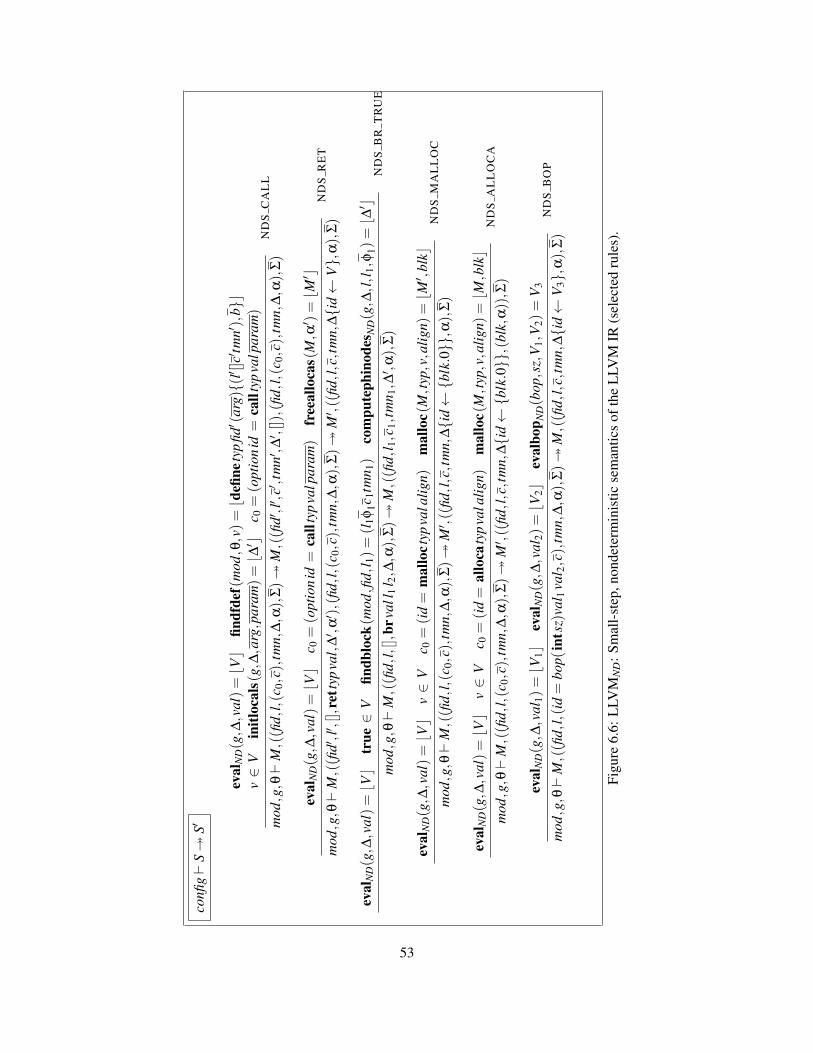
confi
g`
S�
S′
eval
ND(g,∆
,val)=bVc
findf
def(
mod
,θ,v)=bd
efine
typ
fid′ (
arg){(
l′ []c′ tm
n′),
b}c
v∈
Vin
itloc
als(
g,∆,a
rg,p
aram
)=b∆′ c
c 0=(o
ptio
nid
=ca
llty
pva
lpar
am)
mod
,g,θ`
M,((fi
d,l,(c
0,c),t
mn,
∆,α
),Σ)�
M,((fi
d′,l′ ,
c′,t
mn′,∆′ ,[]),(fi
d,l,(c
0,c),t
mn,
∆,α
),Σ)
ND
SC
AL
L
eval
ND(g,∆
,val)=bVc
c 0=(o
ptio
nid
=ca
llty
pva
lpar
am)
free
allo
cas(
M,α′ )=bM′ c
mod
,g,θ`
M,((fi
d′,l′ ,[],r
etty
pva
l,∆′ ,
α′ ),(
fid,l,(
c 0,c),
tmn,
∆,α
),Σ)�
M′ ,((
fid,l,c,t
mn,
∆{i
d←
V},
α),
Σ)
ND
SR
ET
eval
ND(g,∆
,val)=bVc
true∈
Vfin
dblo
ck(m
od,fi
d,l 1)=(l
1φ1c
1tm
n 1)
com
pute
phin
odes
ND(g,∆
,l,l
1,φ
1)=b∆′ c
mod
,g,θ`
M,((fi
d,l,[],b
rval
l 1l 2,∆
,α),
Σ)�
M,((fi
d,l 1,c
1,tm
n 1,∆′ ,
α),
Σ)
ND
SB
RT
RU
E
eval
ND(g,∆
,val)=bVc
v∈
Vc 0
=(i
d=
mal
loct
ypva
lalig
n)m
allo
c(M,t
yp,v,a
lign)
=bM′ ,
blkc
mod
,g,θ`
M,((fi
d,l,(c
0,c),t
mn,
∆,α
),Σ)�
M′ ,((
fid,l,c,t
mn,
∆{i
d←{b
lk.0}},α
),Σ)
ND
SM
AL
LO
C
eval
ND(g,∆
,val)=bVc
v∈
Vc 0
=(i
d=
allo
caty
pva
lalig
n)m
allo
c(M,t
yp,v,a
lign)
=bM
,blkc
mod
,g,θ`
M,((fi
d,l,(c
0,c),t
mn,
∆,α
),Σ)�
M′ ,((
fid,l,c,t
mn,
∆{i
d←{b
lk.0}},(
blk,
α)),Σ)
ND
SA
LL
OC
A
eval
ND(g,∆
,val
1)=bV
1cev
alN
D(g,∆
,val
2)=bV
2cev
albo
p ND(b
op,s
z,V
1,V
2)=
V3
mod
,g,θ`
M,((fi
d,l,(i
d=
bop(
ints
z)va
l 1va
l 2,c),
tmn,
∆,α
),Σ)�
M,((fi
d,l,
c,tm
n,∆{i
d←
V3},α
),Σ)
ND
SB
OP
Figu
re6.
6:L
LVM
ND
:Sm
all-
step
,non
dete
rmin
istic
sem
antic
sof
the
LLV
MIR
(sel
ecte
dru
les)
.
53

From the LLVM Language Reference Manual: “Undefined values indicate to the compiler that the
program is well defined no matter what value is used, giving the compiler more freedom to optimize.”
Semantically, LLVMND treats undef as the set of all values of a given type. For some motivating examples,
consider the following code fragments:
(a) %z = xor i8 undef undef
(b) %x = add i8 0 undef
%z = xor i8 %x %x
(c) %z = or i8 undef 1
(d) br undef %l1 %l2
The value computed for %z in example (a) is the set of all 8-bit integers: because each occurrence of
undef could take on any bit pattern, the set of possible results obtained by xoring them still includes all
8-bit integers. Perhaps surprisingly, example (b) computes the same set of values for %z: one might reason
that no matter which value is chosen for undef, the result of xoring %x with itself would always be 0,
and therefore %z should always be 0. However, while that answer is compatible with the LLVM language
reference (and hence allowed by the nondeterministic semantics), it is also safe to replace code fragment
(b) with %z = undef. The reason is that the LLVM IR adopts a liberal substitution principle: because
%x = undef would be a legitimate replacement for first assignment in (b), it is allowed to substitute undef
for %x throughout, which reduces the assignment to %z to the same code as in (a).
Example (c) shows why the semantics needs arbitrary sets of values. Here, %z evaluates to the set of odd
8-bit integers, which is the result of oring 1 with each element of the set {0, . . . ,255}. This code snippet
could therefore not safely be replaced by %z = undef; however it could be optimized to %z = 1 (or any
other odd 8-bit integer).
Example (d) illustrates the interaction between the set-semantics for local values and the nondeterminism
of the � relation. The control state of the machine holds definite information, so when a branch occurs,
there may be multiple successor states. Similarly, we choose to model memory cells as holding definite
values, so when writing a set to memory, there is one successor state for each possible value that could be
54
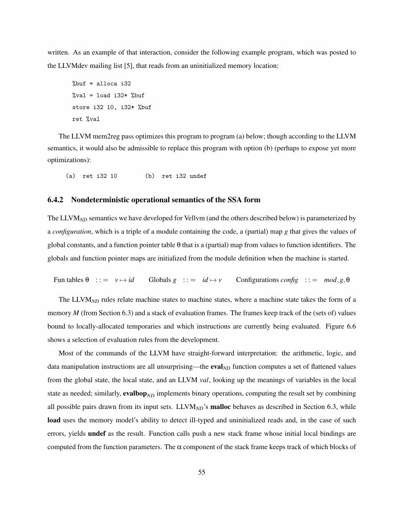
written. As an example of that interaction, consider the following example program, which was posted to
the LLVMdev mailing list [5], that reads from an uninitialized memory location:
%buf = alloca i32
%val = load i32* %buf
store i32 10, i32* %buf
ret %val
The LLVM mem2reg pass optimizes this program to program (a) below; though according to the LLVM
semantics, it would also be admissible to replace this program with option (b) (perhaps to expose yet more
optimizations):
(a) ret i32 10 (b) ret i32 undef
6.4.2 Nondeterministic operational semantics of the SSA form
The LLVMND semantics we have developed for Vellvm (and the others described below) is parameterized by
a configuration, which is a triple of a module containing the code, a (partial) map g that gives the values of
global constants, and a function pointer table θ that is a (partial) map from values to function identifiers. The
globals and function pointer maps are initialized from the module definition when the machine is started.
Fun tables θ : : = v 7→ id Globals g : : = id 7→ v Configurations config : : = mod,g,θ
The LLVMND rules relate machine states to machine states, where a machine state takes the form of a
memory M (from Section 6.3) and a stack of evaluation frames. The frames keep track of the (sets of) values
bound to locally-allocated temporaries and which instructions are currently being evaluated. Figure 6.6
shows a selection of evaluation rules from the development.
Most of the commands of the LLVM have straight-forward interpretation: the arithmetic, logic, and
data manipulation instructions are all unsurprising—the evalND function computes a set of flattened values
from the global state, the local state, and an LLVM val, looking up the meanings of variables in the local
state as needed; similarly, evalbopND implements binary operations, computing the result set by combining
all possible pairs drawn from its input sets. LLVMND’s malloc behaves as described in Section 6.3, while
load uses the memory model’s ability to detect ill-typed and uninitialized reads and, in the case of such
errors, yields undef as the result. Function calls push a new stack frame whose initial local bindings are
computed from the function parameters. The α component of the stack frame keeps track of which blocks of
55
memory are created by the alloca instruction (see rule NDS ALLOCA); these are freed when the function
returns (rule NDS RET). As discussed in Section 4.1, the computephinodesND function in the operational
semantics, as shown, for example, in rule NDS BR TRUE implements “parallel assignment”.
6.4.3 Partiality, preservation, and progress
Throughout the rules the “lift” notation f (x) = bvc indicates that a partial function f is defined on x with
value v. As seen by the frequent uses of lifting, both the nondeterministic and deterministic semantics are
partial—the program may get stuck.
Some of this partiality is related to well-formedness of the SSA program. For example, evalND(g,∆,%x)
is undefined if %x is not bound in ∆. These kinds of errors are ruled out by the static well-formedness
constraints imposed by the LLVM IR (Section 6.2).
In other cases, we have chosen to use partiality in the operational semantics to model certain failure
modes for which the LLVM specification says that the behavior of the program is undefined. These include:
(1) attempting to free memory via a pointer not returned from malloc or that has already been deallocated,
(2) allocating a negative amount of memory, (3) calling load or store on a pointer with bad alignment or
a deallocated address, (4) trying to call a non-function pointer, or (5) trying to execute the unreachable
command. We model these events by stuck states because they correspond to fatal errors that will occur
in any reasonable realization of the LLVM IR by translation to a target platform. Each of these errors is
precisely characterized by a predicate over the machine state (e.g., BadFree(config,S)), and the “allowed”
stuck states are defined to be the disjunction of these predicates:
Stuck(config,S) = BadFree(config,S)
∨ BadLoad(config,S)
∨ . . .
∨ Unreachable(config,S)
To see that the well-formedness properties of the static semantics rule out all but these known error
configurations, we prove the usual preservation and progress theorems for the LLVMND semantics.
Theorem 18 (Preservation for LLVMND). If (config, S) is well formed and config ` S� S′, then (config, S′)
is well formed.
Here, well-formedness includes the static scoping, typing properties, and SSA invariants from Sec-
tion 6.2 for the LLVM code, but also requires that the local mappings ∆ present in all frames of the call
56
stack must be inhabited—each binding contains at least one value v—and that each defined variable that
dominates the current continuation is in ∆’s domain.
That defined variables dominate their uses in the current continuation follows Lemma 11 with consider-
ing the context of the full LLVM IR. To show that the ∆ bindings are inhabited after the step, we prove that
(1) non-undef values V are singletons; (2) undefined values from constants typundef contain all possible
values of first class types typ; (3) undefined values from loading uninitialized memory or incompatible phys-
ical data contain at least paddings indicating errors; (4) evaluation of non-deterministic values by evalbopND
returns non-empty sets of values given non-empty inputs.
Theorem 19 (Progress for LLVMND). If the pair (config, S) is well formed, then either S has terminated
successfully or Stuck(config,S) or there exists S’ such that config ` S� S′.
This theorem holds because in a well-formed machine state, evalND always returns a non-empty value
set V; moreover jump targets and internal functions are always present.
6.4.4 Deterministic refinements
Although the LLVMND semantics is useful for reasoning about the validity of LLVM program transforma-
tions, Vellvm provides a LLVMD, a deterministic, small-step refinement, along with two large-step opera-
tional semantics LLVM∗DFn and LLVM∗DB.
These different deterministic semantics are useful for several reasons: (1) they provide the basis for
testing LLVM programs with a concrete implementation of memory (see the discussion about Vellvm’s
extracted interpreter in the next Section), (2) proving that LLVMD is an instance of the LLVMND and relating
the small-step rules to the large-step ones provides validation of all of the semantics (i.e., we found bugs in
Vellvm by formalizing multiple semantics and trying to prove that they are related), and (3) the small- and
large-step semantics have different applications when reasoning about LLVM program transformations.
Unlike LLVMND, the frames for these semantics map identifiers to single values, not sets, and the op-
erational rules call deterministic variants of the nondeterministic counterparts (e.g., eval instead of evalND).
To resolve the nondeterminism from undef and faulty memory operations, these semantics fix a concrete
interpretation as follows:
• undef is treated as a zeroinitializer
• Reading uninitialized memory returns zeroinitializer
57
These choices yield unrealistic behaviors compared to what one might expect from running a LLVM
program against a C-style runtime system, but the cases where this semantics differs correspond to unsafe
programs. There are still many programs, namely those compiled to LLVM from type-safe languages,
whose behaviors under this semantics should agree with their realizations on target platforms. Despite these
differences from LLVMND, LLVMD also has the preservation and progress properties.
Big-step semantics Vellvm also provides big-step operational semantics LLVM∗DFn, which evaluates a
function call as one large step, and LLVM∗DB, which evaluates each sub-block—i.e., the code between
two function calls—as one large step. Big-step semantics are useful because compiler optimizations often
transform multiple instructions or blocks within a function in one pass. Such transformations do not preserve
the small-step semantics, making it hard to create simulations that establish correctness properties.
As a simple application of the large-step semantics, consider trying to prove the correctness of a transfor-
mation that re-orders program statements that do not depend on one another. For example, the following two
programs result in the same states if we consider their execution as one big-step, although their intermediate
states do not match in terms of the small-step semantics.
(a) %x = add i32 %a, %b (b) %y = load i32* %p
%y = load i32* %p %x = add i32 %a, %b
The proof of this claim in Vellvm uses the LLVM∗DB rules to hide the details about the intermediate
states. To handle memory effects, we use a simulation relation that uses symbolic evaluation [52] to define
the equivalence of two memory states. The memory contents are defined abstractly in terms of the program
operations by recording the sequence of writes. Using this technique, we defined a simple translation
validator to check whether the semantics of two programs are equivalent with respect to such re-orderings
execution. For each pair of functions, the validator ensures that their control-flow graphs match, and that all
corresponding sub-blocks are equivalent in terms of their symbolic evaluation. This approach is similar to
the translation validation used in prior work for verifying instruction scheduling optimizations [68].
Although this is a simple application of Vellvm’s large-step semantics, proving correctness of other
program transformations such as dead expression elimination and constant propagation follow a similar
pattern—the difference is that, rather than checking that two memories are syntactically equivalent according
to the symbolic evaluation, we must check them with respect to a more semantic notion of equivalence [52].
58
Relationships among the semantics Figure 6.5 illustrates how these various operational semantics relate
to one another. Vellvm provides proofs that LLVM∗DB simulates LLVM∗DFn and that LLVM∗DFn simulates
LLVMD. In these proofs, simulation is taken to mean that the machine states are syntactically identical at
corresponding points during evaluation. For example, the state at a function call of a program running on
the LLVM∗DFn semantics matches the corresponding state at the function call reached in LLVMD. Note that
in the deterministic setting, one-direction simulation implies bisimulation [42]. Moreover, LLVMD is a
refinement instance of the nondeterministic LLVMND semantics.
These relations are useful because the large-step semantics induce different proof styles than the small-
step semantics: in particular, the induction principles obtained from the large step semantics allow one to
gloss over insignificant details of the small step semantics.
Omitted details The operational semantics supports external function calls by assuming that their behav-
ior is specified by axioms; the implementation applies these axioms to transition program states upon calling
external functions.
6.5 Extracting an Interpreter
To test Vellvm’s operational semantics for the LLVM IR, we used Coq’s code extraction facilities to obtain
an interpreter for executing the LLVM distribution’s regression test suite. Extracting such an interpreter
is one of the main motivations for developing a deterministic semantics, because the evaluation under the
nondeterministic semantics cannot be directly compared against actual runs of LLVM IR programs.
Unfortunately, the small-step deterministic semantics LLVMD is defined relationally in the logical frag-
ment of Coq, which is convenient for proofs, but can not be used to extract code. Therefore, Vellvm provides
yet another operational semantics, LLVMInterp, which is a deterministic functional interpreter implemented
in the computational fragment of Coq. LLVMInterp is proved to be bisimilar to LLVMD, so we can port
results between the two semantics.
Although one could run this extracted interpreter directly, doing so is not efficient. First, integers with
arbitrary bit-width are inductively defined in Coq. This yields easy proof principles, but does not give
an efficient runtime representation; floating point operations are defined axiomatically. To remedy these
problems, at extraction we realize Vellvm’s integer and floating point values by efficient C++ libraries
that are a standard part of the LLVM distribution. Second, the memory model implementation of Vellvm
59
maintains memory blocks and their associated metadata as functional lists, and it converts between byte-
list and value representations at each memory access. Using the extracted data-structures directly incurs
tremendous performance overhead, so we replaced the memory operations of the memory model with native
implementations from the C standard library. A value v in local mappings δ is boxed, and it is represented
by a reference to memory that stores its content.
Our implementation faithfully runs 134 out of the 145 tests from the LLVM regression suite that lli,
the LLVM distribution interpreter, can run. The missing tests cover instructions (like variable arguments)
that are not implemented in Vellvm.
Although replacing the Coq data-structures by native ones weakens the absolute correctness guarantees
one would expect from an extracted interpreter, this exercise is still valuable. In the course of carrying out
this experiment, we found one severe bug in the semantics: the br instruction inadvertently swapped the
true and false branches.
60
Chapter 7
Verified SoftBound
To demonstrate the effectiveness of Vellvm, our first application of Vellvm is a verified instance of Soft-
Bound [50, 51], a previously proposed program transformation that hardens C programs against spatial
memory safety violations (e.g., buffer overflows, array indexing errors, and pointer arithmetic errors). Soft-
Bound works by first compiling C programs into the LLVM IR and then instrumenting the program with
instructions that propagate and check per-pointer metadata. SoftBound maintains base and bound metadata
with each pointer, shadowing loads and stores of pointer with parallel loads and stores of their associated
metadata. This instrumentation ensures that each pointer dereferenced is within bounds and aborts the pro-
gram otherwise.
The original SoftBound paper includes a mechanized proof that validates the correctness of this idea,
but it is not complete. In particular, the proof is based on a subset of a C-like language with only straight-
line commands and non-aggregate types, in contrast a SoftBound implementation needs to consider all of
the LLVM IR shown in Figure 6.1 and Figure 6.2, the memory model, and the full operational semantics
of the LLVM IR. Also the original proof ensures the correctness only with respect to a specification that
the SoftBound instrumentation must implement, but it does not prove the correctness of the instrumentation
pass itself. Moreover, the specification requires that every temporary must contain metadata, not just pointer
temporaries.
Using Vellvm to verify SoftBound This chapter describes how we use Vellvm to formally verify the
correctness of the SoftBound instrumentation pass with respect to the LLVM semantics, demonstrating that
the promised spatial memory safety property is achieved. Moreover, Vellvm allows us to extract a verified
61

OCaml implementation of the transformation from Coq. The end result is a compiler pass that is formally
verified to transform a program in the LLVM IR into a program augmented with sufficient checking code
such that it will dynamically detect and prevent all spatial memory safety violations.
SoftBound is a good test case for the Vellvm framework. It is a non-trivial translation pass that never-
theless only inserts code, thereby making it easier to prove correct. SoftBound’s intended use is to prevent
security vulnerabilities, so bugs in its implementation can potentially have severe consequences. Also, the
existing SoftBound implementation already uses the LLVM.
Modifications to SoftBound since the original paper As described in the original paper, SoftBound
modifies function signatures to pass metadata associated with the pointer parameters or returned pointers.
To improve the robustness of the tool, we transitioned to an implementation that instead passes all pointer
metadata on a shadow stack [50]. This has two primary advantages. The first is that this design simplifies
the implementation while simultaneously better supporting indirect function calls (via function pointers)
and more robustly handling improperly declared function prototypes. The second is that it also simplifies
the proofs.
7.1 Formalizing SoftBound for the LLVM IR
The SoftBound correctness proof has the following high-level structure:
1. We define a nonstandard operational semantics SBspec for the LLVM IR. This semantics “builds in”
the safety properties that should be enforced by a correct implementation of SoftBound. It uses meta-
level datastructures to implement the metadata and meta-level functions to define the semantics of the
bounds checks.
2. We prove that an LLVM program P, when run on the SBspec semantics, has no spatial safety viola-
tions.
3. We define a translation pass SBtrans(−) that instruments the LLVM code to propagate metadata.
4. We prove that if SBtrans(P) = bP′c then P’, when run on the LLVMD, simulates P running on SBspec.
62
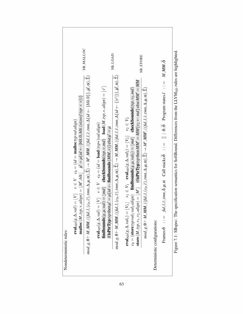
Non
dete
rmin
istic
rule
s: eval
ND(g,∆
,val)=bVc
v∈
Vc 0
=(i
d=
mal
loct
ypva
lalig
n)m
allo
c(M,t
yp,v,a
lign)
=bM′ ,
blkc
µ′=
µ{id←
[blk.0,b
lk.(
size
oft
yp×
v))}
mod
,g,θ`
M,M
M,((fi
d,l,(c
0,c),t
mn,
∆,µ,α
),Σ)�
M′ ,
MM,((fi
d,l,
c,tm
n,∆{i
d←{b
lk.0}},µ′ ,
α),
Σ)
SB
MA
LL
OC
eval
ND(g,∆
,val)=bVc
v∈
Vc 0
=(i
d=
load
(typ∗)
vala
lign)
findb
ound
s(g,
µ,va
l)=bm
dcch
eckb
ound
s(ty
p,v,
md)
load
(M,t
yp,v,a
lign)
=bv′ c
ifis
PtrT
ypty
pth
enµ′=
µ{id←
findb
ound
s(M
M,v)}
else
µ′=
µ
mod
,g,θ`
M,M
M,((fi
d,l,(c
0,c),t
mn,
∆,µ,α
),Σ)�
M,M
M,((fi
d,l,
c,tm
n,∆{i
d←{|
v′|}},
µ′,α
),Σ)
SB
LO
AD
eval
ND(g,∆
,val
1)=bV
1cv 1∈
V1
eval
ND(g,∆
,val
2)=bV
2cv 2∈
V2
c 0=(s
tore
typ
val 1
val 2
alig
n)fin
dbou
nds(
g,µ,
val 2)=bm
dcch
eckb
ound
s(ty
p,v 2,m
d)st
ore(
M,t
yp,v
1,v 2,a
lign)
=bM′ c
ifis
PtrT
ypty
pth
enM
M′ =
MM{v
2←
md}
else
MM′ =
MM
mod
,g,θ`
M,M
M,((fi
d,l,(c
0,c),t
mn,
∆,µ,α
),Σ)�
M′ ,
MM′ ,((
fid,l,c,t
mn,
∆,µ,α
),Σ)
SB
ST
OR
E
Det
erm
inis
ticco
nfigu
ratio
ns:
Fram
esσ
::=
fid,l,c,t
mn,
δ,µ,α
Cal
lsta
cksσ
::=
[]|
σ,σ
Prog
ram
stat
ess
::=
M,M
M,σ
Figu
re7.
1:SB
spec
:The
spec
ifica
tion
sem
antic
sfo
rSof
tBou
nd.D
iffer
ence
sfr
omth
eL
LVM
ND
rule
sar
ehi
ghlig
hted
.
63
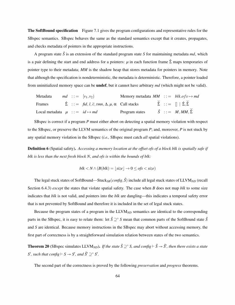
The SoftBound specification Figure 7.1 gives the program configurations and representative rules for the
SBspec semantics. SBspec behaves the same as the standard semantics except that it creates, propagates,
and checks metadata of pointers in the appropriate instructions.
A program state S is an extension of the standard program state S for maintaining metadata md, which
is a pair defining the start and end address for a pointers: µ in each function frame Σ maps temporaries of
pointer type to their metadata; MM is the shadow heap that stores metadata for pointers in memory. Note
that although the specification is nondeterministic, the metadata is deterministic. Therefore, a pointer loaded
from uninitialized memory space can be undef, but it cannot have arbitrary md (which might not be valid).
Metadata md : : = [v1,v2) Memory metadata MM : : = blk.o f s 7→ md
Frames Σ : : = fid, l, c, tmn, ∆, µ, α Call stacks Σ : : = [] | Σ, Σ
Local metadata µ : : = id 7→ md Program states S : : = M, MM, Σ
SBspec is correct if a program P must either abort on detecting a spatial memory violation with respect
to the SBspec, or preserve the LLVM semantics of the original program P; and, moreover, P is not stuck by
any spatial memory violation in the SBspec (i.e., SBspec must catch all spatial violations).
Definition 6 (Spatial safety). Accessing a memory location at the offset ofs of a block blk is spatially safe if
blk is less than the next fresh block N, and ofs is within the bounds of blk:
blk < N∧ (B(blk) = bsizec → 0≤ ofs < size)
The legal stuck states of SoftBound—StuckSB(config, S) include all legal stuck states of LLVMND (recall
Section 6.4.3) except the states that violate spatial safety. The case when B does not map blk to some size
indicates that blk is not valid, and pointers into the blk are dangling—this indicates a temporal safety error
that is not prevented by SoftBound and therefore it is included in the set of legal stuck states.
Because the program states of a program in the LLVMND semantics are identical to the corresponding
parts in the SBspec, it is easy to relate them: let S ⊇◦ S mean that common parts of the SoftBound state S
and S are identical. Because memory instructions in the SBspec may abort without accessing memory, the
first part of correctness is by a straightforward simulation relation between states of the two semantics.
Theorem 20 (SBspec simulates LLVMND). If the state S⊇◦ S, and config ` S� S′, then there exists a state
S′, such that config ` S� S′, and S′ ⊇◦ S′.
The second part of the correctness is proved by the following preservation and progress theorems.
64
Theorem 21 (Preservation for SBspec).
If (config, S) is well formed, and config ` S� S′, then (config, S′) is well formed.
Here, SBspec well-formedness strengthens the invariants for LLVMND by requiring that if any id defined
in ∆ is of pointer type, then µ contains its metadata and a spatial safety invariant: all bounds in µs of function
frames and MM must be memory ranges within which all memory addresses are spatially safe.
The interesting part is proving that the spatial safety invariant is preserved. It holds initially, because a
program’s initial frame stack is empty, and we assume that MM is also empty. The other cases depend on
the rules in Figure 7.1.
The rule SB MALLOC, which allocates the number v of elements with typ at a memory block blk, updates
the metadata of id with the start address that is the beginning of blk, and the end address that is at the offset
blk.(sizeo f typ × v) in the same block. LLVM’s memory model ensures that the range of memory is valid.
The rule SB LOAD reads from a pointer val with runtime data v, finds the md of the pointer, and
ensures that v is within the md via checkbounds. If the val is an identifier, findbounds simply returns
the identifier’s metadata from µ, which must be a spatial safe memory range. If val is a constant of pointer
type, findbounds returns bounds as the following. For global pointers, findbounds returns bounds derived
from their types because globals must be allocated before a program starts. For pointers converted from
some constant integers by inttoptr, it conservatively returns the bounds [null,null) to indicate a potentially
invalid memory range. For a pointer cnst1 derived from an other constant pointer cnst2 by bitcase or
getelementptr, findbounds returns the same bound of cnst2 for cnst1. Note that {|v′|} denotes conversion
from a deterministic value to a nondeterministic value.
If the load reads a pointer-typed value v from memory, the rule finds its metadata in MM and updates
the local metadata mapping µ. If MM does not contain any metadata indexed by v, that means the pointer
being loaded was not stored with valid bounds, so findbounds returns [null,null) to ensure the spatial safety
invariant. Similarly, the rule SB STORE checks whether the address to be stored to is in bounds and, if storing
a pointer, updates MM accordingly. SoftBound disallows dereferencing a pointer that was converted from an
integer, even if that integer was originally obtained from a valid pointer. Following the same design choice,
findbounds returns [null,null) for pointers cast from integers. checkbounds fails when a program accesses
such pointers.
Theorem 22 (Progress for SBspec). If S1 is well-formed, then either S1 is a final state, or S1 is a legal stuck
state, or there exists a S2 such that config ` S1� S2.
65
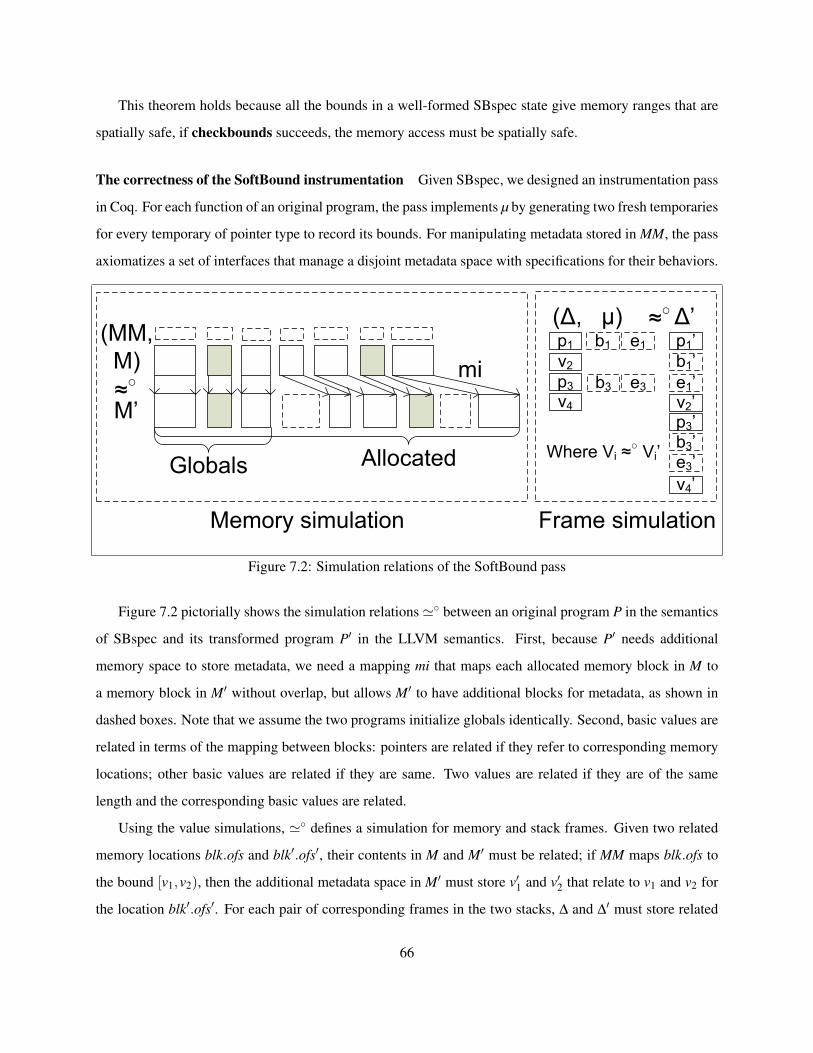
This theorem holds because all the bounds in a well-formed SBspec state give memory ranges that are
spatially safe, if checkbounds succeeds, the memory access must be spatially safe.
The correctness of the SoftBound instrumentation Given SBspec, we designed an instrumentation pass
in Coq. For each function of an original program, the pass implements µ by generating two fresh temporaries
for every temporary of pointer type to record its bounds. For manipulating metadata stored in MM, the pass
axiomatizes a set of interfaces that manage a disjoint metadata space with specifications for their behaviors.
Globals Allocated
M’
p1
v2
p3v4
b1 e1
b3 e3
p1’
v2’p3’
v4’
b1’e1’
b3’e3’
(Δ, μ) Δ’≈○
≈○
(MM,M)
Memory simulation Frame simulation
mi
Where Vi ≈○ Vi’
Figure 7.2: Simulation relations of the SoftBound pass
Figure 7.2 pictorially shows the simulation relations'◦ between an original program P in the semantics
of SBspec and its transformed program P′ in the LLVM semantics. First, because P′ needs additional
memory space to store metadata, we need a mapping mi that maps each allocated memory block in M to
a memory block in M′ without overlap, but allows M′ to have additional blocks for metadata, as shown in
dashed boxes. Note that we assume the two programs initialize globals identically. Second, basic values are
related in terms of the mapping between blocks: pointers are related if they refer to corresponding memory
locations; other basic values are related if they are same. Two values are related if they are of the same
length and the corresponding basic values are related.
Using the value simulations, '◦ defines a simulation for memory and stack frames. Given two related
memory locations blk.ofs and blk′.ofs′, their contents in M and M′ must be related; if MM maps blk.ofs to
the bound [v1,v2), then the additional metadata space in M′ must store v′1 and v′2 that relate to v1 and v2 for
the location blk′.ofs′. For each pair of corresponding frames in the two stacks, ∆ and ∆′ must store related
66
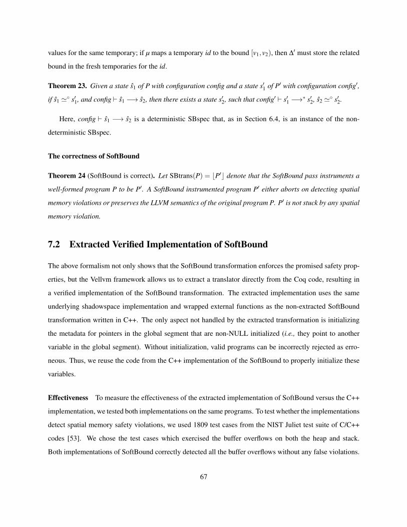
values for the same temporary; if µ maps a temporary id to the bound [v1,v2), then ∆′ must store the related
bound in the fresh temporaries for the id.
Theorem 23. Given a state s1 of P with configuration config and a state s′1 of P′ with configuration config′,
if s1 '◦ s′1, and config ` s1 −→ s2, then there exists a state s′2, such that config′ ` s′1 −→∗ s′2, s2 '◦ s′2.
Here, config ` s1 −→ s2 is a deterministic SBspec that, as in Section 6.4, is an instance of the non-
deterministic SBspec.
The correctness of SoftBound
Theorem 24 (SoftBound is correct). Let SBtrans(P) = bP′c denote that the SoftBound pass instruments a
well-formed program P to be P′. A SoftBound instrumented program P′ either aborts on detecting spatial
memory violations or preserves the LLVM semantics of the original program P. P′ is not stuck by any spatial
memory violation.
7.2 Extracted Verified Implementation of SoftBound
The above formalism not only shows that the SoftBound transformation enforces the promised safety prop-
erties, but the Vellvm framework allows us to extract a translator directly from the Coq code, resulting in
a verified implementation of the SoftBound transformation. The extracted implementation uses the same
underlying shadowspace implementation and wrapped external functions as the non-extracted SoftBound
transformation written in C++. The only aspect not handled by the extracted transformation is initializing
the metadata for pointers in the global segment that are non-NULL initialized (i.e., they point to another
variable in the global segment). Without initialization, valid programs can be incorrectly rejected as erro-
neous. Thus, we reuse the code from the C++ implementation of the SoftBound to properly initialize these
variables.
Effectiveness To measure the effectiveness of the extracted implementation of SoftBound versus the C++
implementation, we tested both implementations on the same programs. To test whether the implementations
detect spatial memory safety violations, we used 1809 test cases from the NIST Juliet test suite of C/C++
codes [53]. We chose the test cases which exercised the buffer overflows on both the heap and stack.
Both implementations of SoftBound correctly detected all the buffer overflows without any false violations.
67
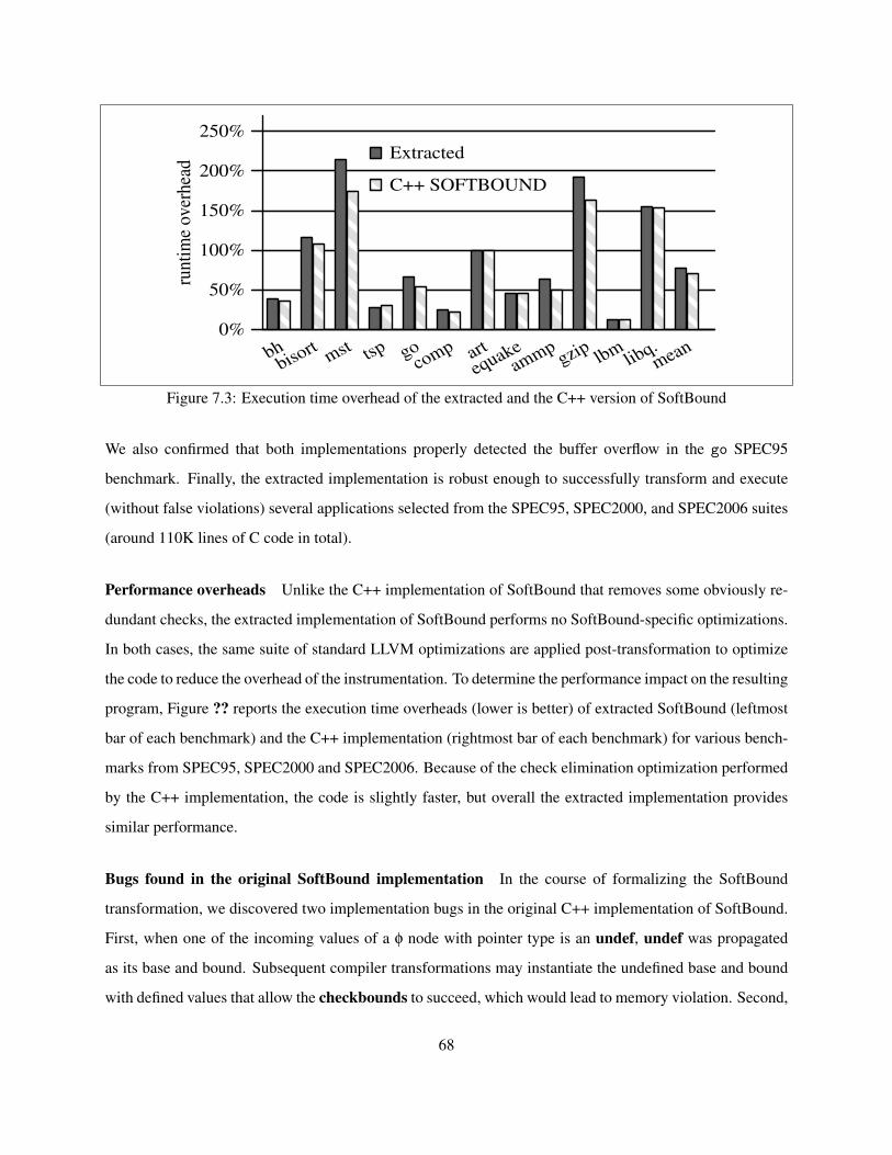
0%
50%
100%
150%
200%
250%
run
tim
e o
ver
hea
d
Extracted
C++ SOFTBOUND
bhbiso
rt mst tsp gocomp art
equakeammp
gzip lbmlib
q.mean
Figure 7.3: Execution time overhead of the extracted and the C++ version of SoftBound
We also confirmed that both implementations properly detected the buffer overflow in the go SPEC95
benchmark. Finally, the extracted implementation is robust enough to successfully transform and execute
(without false violations) several applications selected from the SPEC95, SPEC2000, and SPEC2006 suites
(around 110K lines of C code in total).
Performance overheads Unlike the C++ implementation of SoftBound that removes some obviously re-
dundant checks, the extracted implementation of SoftBound performs no SoftBound-specific optimizations.
In both cases, the same suite of standard LLVM optimizations are applied post-transformation to optimize
the code to reduce the overhead of the instrumentation. To determine the performance impact on the resulting
program, Figure ?? reports the execution time overheads (lower is better) of extracted SoftBound (leftmost
bar of each benchmark) and the C++ implementation (rightmost bar of each benchmark) for various bench-
marks from SPEC95, SPEC2000 and SPEC2006. Because of the check elimination optimization performed
by the C++ implementation, the code is slightly faster, but overall the extracted implementation provides
similar performance.
Bugs found in the original SoftBound implementation In the course of formalizing the SoftBound
transformation, we discovered two implementation bugs in the original C++ implementation of SoftBound.
First, when one of the incoming values of a φ node with pointer type is an undef, undef was propagated
as its base and bound. Subsequent compiler transformations may instantiate the undefined base and bound
with defined values that allow the checkbounds to succeed, which would lead to memory violation. Second,
68

the base and bound of constant pointer (typ∗)null was set to be (typ∗)null and (typ∗)null+ sizeof (typ),
allowing dereferences of null or pointers pointing to an offset from null. Either of these bugs could have
resulted in faulty checking and thus expose the program to the spatial violations that SoftBound was designed
to prevent. These bugs underscore the importance of a formally verified and extracted implementation to
avoid such bugs.
69
Chapter 8
Verified SSA Construction for LLVM
Chapter 5 described the proof techniques we have developed for verifying SSA-based program transfor-
mations in the context of Vminus. This chapter demonstrates that these proof techniques can be used for
practical compiler optimizations in Vellvm: verifying the most performance-critical optimization pass in
LLVM’s compilation strategy—the mem2reg pass.
8.1 The mem2reg Optimization Pass
LLVM provides a large suite of optimization passes, including aggressive dead code elimination (ADCE),
global value numbering (GVN), partial redundancy elimination (PRE), and sparse conditional constant prop-
agation (SCCP) among others. Figure 2.3 shows the tool chain of the LLVM compiler. Each transformation
pass consumes and produces code in this SSA form, and they typically have the flavor of the code transfor-
mations described above in Chapter 5.
A critical piece of LLVM’s compilation strategy is the mem2reg pass, which takes code that is “trivially”
in SSA form and converts it into a minimal, pruned SSA program [62]. This strategy simplifies LLVM’s
many front ends by moving work in to mem2reg. An SSA form is “minimal” if each φ is placed only at
the dominance frontier of the definitions of the φ node’s incoming variables [28]. A minimal SSA form is
“pruned” if it contains only live φ nodes [62]. This pass enables many subsequent optimizations (and, in
particular, backend optimizations such as register allocation) to work effectively.
Figure 8.2 demonstrates the importance of the mem2reg pass for LLVM’s generated code performance.
In our experiments, running only the mem2reg pass yields a 81% speedup (on average) compared to LLVM
70

BackendsLLVM SSA
with φ-nodes
ADCE, GVN,
PRE, SCCP, ...
Frontends
w/o SSA
construction
LLVM SSA
w/o φ-nodes mem2reg
Figure 8.1: The tool chain of the LLVM compiler
without any optimizations; doing the full suite of -O1 level optimizations (which includes mem2reg) yields
a speedup of 102%, which means that mem2reg alone captures all but %12 of the benefit of the -O1
level optimizations. Comparison with -O3 optimizations yields similar results. These observations make
mem2reg an obvious target for our verification efforts.
The “trivial” SSA form is generated directly by compiler front ends, and it uses the alloca instruction to
allocate stack space for every source-program local variable and temporary needed. In this form, an LLVM
SSA variable is used either only locally to access those stack slots, in which case the variable is never live
across two basic blocks, or it is a reference to the stack slot, whose lifetime corresponds to the source-level
variable’s scope. These constraints mean that no φ instructions are needed—it is extremely straightforward
for a front end to generate code in this form.
As an example, consider this C program (which is a running example through this chapter):
int i = 0;
while (i<=100) i++;
return i;
The “trivial” SSA form that might be produced by the frontend of a compiler is shown in the left-most
column of Figure 8.4 and Figure 8.5. The r0 := allocaint instruction on the first line allocates space for the
source variable i, and r0 is a reference from which local load and store instructions access i’s contents.
The mem2reg pass converts promotable uses of stack-allocated variables to SSA temporaries.
Definition 7 (Promotable allocations). An allocation r is promotable in f , written promotable( f ,r), if
r := alloca typ is in the entry block of f , and r does not escape (r is not stored into memory; ∀insn ∈
f , insnusesr =⇒ insn is a store or load).
71
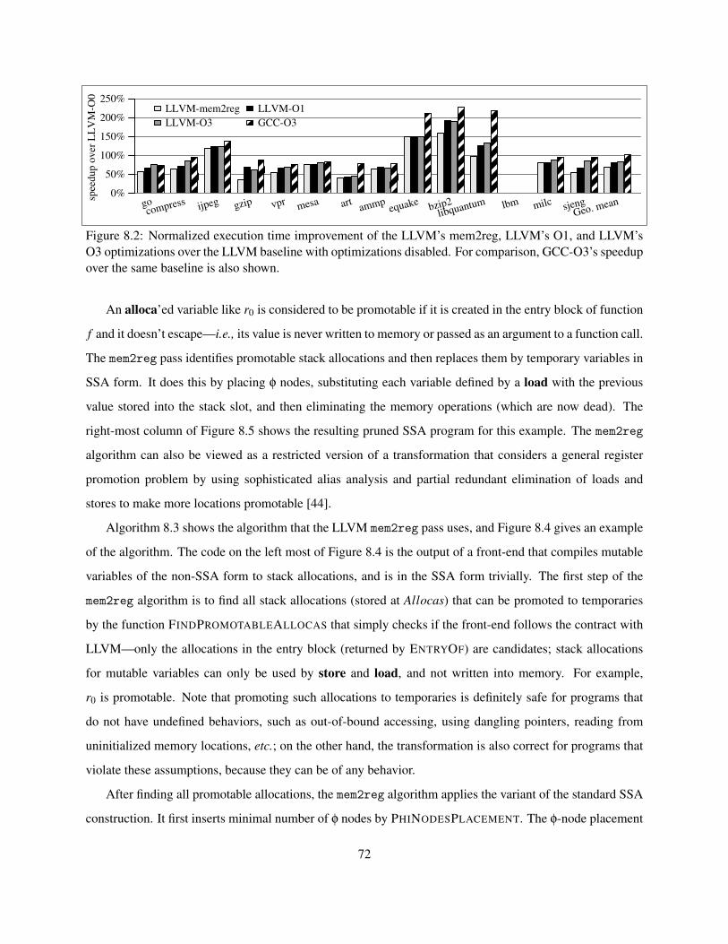
0%
50%
100%
150%
200%
250%sp
eedup o
ver
LL
VM
-O0
LLVM-mem2reg LLVM-O1
LLVM-O3 GCC-O3
gocompress ijpeg gzip vpr mesa art
ammpequake
bzip2libquantum lbm milc sjeng
Geo. mean
Figure 8.2: Normalized execution time improvement of the LLVM’s mem2reg, LLVM’s O1, and LLVM’sO3 optimizations over the LLVM baseline with optimizations disabled. For comparison, GCC-O3’s speedupover the same baseline is also shown.
An alloca’ed variable like r0 is considered to be promotable if it is created in the entry block of function
f and it doesn’t escape—i.e., its value is never written to memory or passed as an argument to a function call.
The mem2reg pass identifies promotable stack allocations and then replaces them by temporary variables in
SSA form. It does this by placing φ nodes, substituting each variable defined by a load with the previous
value stored into the stack slot, and then eliminating the memory operations (which are now dead). The
right-most column of Figure 8.5 shows the resulting pruned SSA program for this example. The mem2reg
algorithm can also be viewed as a restricted version of a transformation that considers a general register
promotion problem by using sophisticated alias analysis and partial redundant elimination of loads and
stores to make more locations promotable [44].
Algorithm 8.3 shows the algorithm that the LLVM mem2reg pass uses, and Figure 8.4 gives an example
of the algorithm. The code on the left most of Figure 8.4 is the output of a front-end that compiles mutable
variables of the non-SSA form to stack allocations, and is in the SSA form trivially. The first step of the
mem2reg algorithm is to find all stack allocations (stored at Allocas) that can be promoted to temporaries
by the function FINDPROMOTABLEALLOCAS that simply checks if the front-end follows the contract with
LLVM—only the allocations in the entry block (returned by ENTRYOF) are candidates; stack allocations
for mutable variables can only be used by store and load, and not written into memory. For example,
r0 is promotable. Note that promoting such allocations to temporaries is definitely safe for programs that
do not have undefined behaviors, such as out-of-bound accessing, using dangling pointers, reading from
uninitialized memory locations, etc.; on the other hand, the transformation is also correct for programs that
violate these assumptions, because they can be of any behavior.
After finding all promotable allocations, the mem2reg algorithm applies the variant of the standard SSA
construction. It first inserts minimal number of φ nodes by PHINODESPLACEMENT. The φ-node placement
72
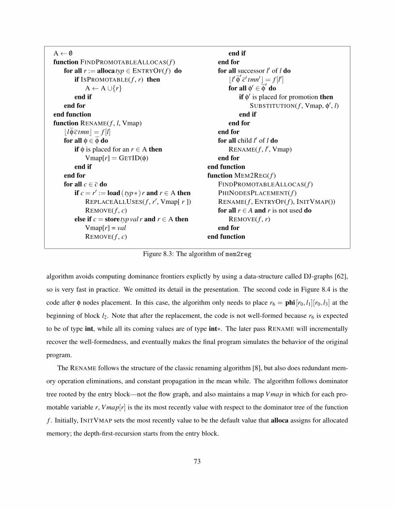
A← /0
function FINDPROMOTABLEALLOCAS( f )for all r := alloca typ ∈ ENTRYOF( f ) do
if ISPROMOTABLE( f , r) thenA← A ∪{r}
end ifend for
end functionfunction RENAME( f , l, Vmap)blφctmnc= f [l]for all φ ∈ φ do
if φ is placed for an r ∈ A thenVmap[r] = GETID(φ)
end ifend forfor all c ∈ c do
if c = r′ := load( typ∗)r and r ∈ A thenREPLACEALLUSES( f , r′, Vmap[ r ])REMOVE( f , c)
else if c = store typval r and r ∈ A thenVmap[r] = valREMOVE( f , c)
end ifend forfor all successor l′ of l dobl′ φ′ c′ tmn′c= f [l′]for all φ′ ∈ φ
′ doif φ′ is placed for promotion then
SUBSTITUTION( f , Vmap, φ′, l)end if
end forend forfor all child l′ of l do
RENAME( f , l′, Vmap)end for
end functionfunction MEM2REG( f )
FINDPROMOTABLEALLOCAS( f )PHINODESPLACEMENT( f )RENAME( f , ENTRYOF( f ), INITVMAP())for all r ∈ A and r is not used do
REMOVE( f , r)end for
end function
Figure 8.3: The algorithm of mem2reg
algorithm avoids computing dominance frontiers explictly by using a data-structure called DJ-graphs [62],
so is very fast in practice. We omitted its detail in the presentation. The second code in Figure 8.4 is the
code after φ nodes placement. In this case, the algorithm only needs to place r6 = phi [r0, l1][r0, l3] at the
beginning of block l2. Note that after the replacement, the code is not well-formed because r6 is expected
to be of type int, while all its coming values are of type int∗. The later pass RENAME will incrementally
recover the well-formedness, and eventually makes the final program simulates the behavior of the original
program.
The RENAME follows the structure of the classic renaming algorithm [8], but also does redundant mem-
ory operation eliminations, and constant propagation in the mean while. The algorithm follows dominator
tree rooted by the entry block—not the flow graph, and also maintains a map V map in which for each pro-
motable variable r, V map[r] is the its most recently value with respect to the dominator tree of the function
f . Initially, INITVMAP sets the most recently value to be the default value that alloca assigns for allocated
memory; the depth-first-recursion starts from the entry block.
73
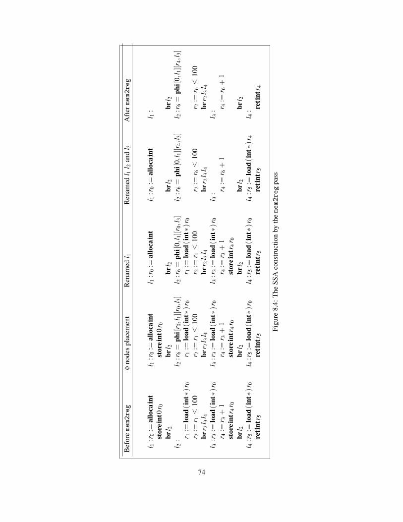
Bef
oremem2reg
φno
des
plac
emen
tR
enam
edl 1
Ren
amed
l 1l 2
and
l 3A
ftermem2reg
l 1:r
0:=
allo
cain
tst
orei
nt0
r 0br
l 2l 2
: r 1:=
load
(int∗)
r 0r 2
:=r 1≤
100
brr 2
l 3l 4
l 3:r
3:=
load
(int∗)
r 0r 4
:=r 3
+1
stor
eint
r 4r 0
brl 2
l 4:r
5:=
load
(int∗)
r 0re
tint
r 5
l 1:r
0:=
allo
cain
tst
orei
nt0
r 0br
l 2l 2
:r6=
phi[
r 0,l
1][r
0,l 3]
r 1:=
load
(int∗)
r 0r 2
:=r 1≤
100
brr 2
l 3l 4
l 3:r
3:=
load
(int∗)
r 0r 4
:=r 3
+1
stor
eint
r 4r 0
brl 2
l 4:r
5:=
load
(int∗)
r 0re
tint
r 5
l 1:r
0:=
allo
cain
t
brl 2
l 2:r
6=
phi[
0,l 1][
r 0,l
3]r 1
:=lo
ad(i
nt∗)
r 0r 2
:=r 1≤
100
brr 2
l 3l 4
l 3:r
3:=
load
(int∗)
r 0r 4
:=r 3
+1
stor
eint
r 4r 0
brl 2
l 4:r
5:=
load
(int∗)
r 0re
tint
r 5
l 1:r
0:=
allo
cain
t
brl 2
l 2:r
6=
phi[
0,l 1][
r 4,l
3]
r 2:=
r 6≤
100
brr 2
l 3l 4
l 3: r 4
:=r 6
+1
brl 2
l 4:r
5:=
load
(int∗)
r 4re
tint
r 5
l 1: br
l 2l 2
:r6=
phi[
0,l 1][
r 4,l
3]
r 2:=
r 6≤
100
brr 2
l 3l 4
l 3: r 4
:=r 6
+1
brl 2
l 4: re
tint
r 4
Figu
re8.
4:T
heSS
Aco
nstr
uctio
nby
themem2reg
pass
74
At each visited block lφctmn, the algorithm first checks if there is any φ placed for a promotable
temporary r. If so, the algorithm takes the temporary defined by the φ as the most recent value for r in
the map V map. Then, for each command c, if c is a load from a promotable temporary r to r′, then the
algorithm replaces all the uses of r′ by the most recent value of r stored in V map, then remove the c; if c is
a store to a promotable temporary r with a value val, then the algorithm sets val to be the most recent value
for r, then removes the c; otherwise, the algorithm does nothing. At the end, it examines all the successors
(in term of the control-flow graph) of l to see if there are any φ nodes whose operands need to be properly
renamed, and then recursively renames all children blocks (in term of the dominator tree) of l.
After the renaming of block l1, the store store int0r0 in block l1 was removed; because at the end of
block l1 the recent value of r1 is 0 that is from the removed store, in the φ of l2 that is the successor of l1,
the algorithm replaced the r0 corresponding to l1 by 0. The next code in Figure 8.4 shows the depth-first-
search-based renaming up to one leaf of the dominator tree when all the blocks l1, l2 and l3 were renamed.
Note that the algorithm does not change the incoming value of the φ node in block l2 when RENAME visited
l2, but changed the r0 of the incoming block l3 to be r4 when RENAME visited the end of the block l3 whose
successor is l2. The other observation is that although the code is well-formed, it does not preserve the
meaning of its original program because the value of r5 is read from the uninitialized location r0, while in
the original program r5 should be 100 at the return of the program.
After renaming, the last step of the mem2reg pass is checking if there is any promotable temporaries r
which is not used at all, and, therefore, can be safely removed. As shown in the right most code of Figure 8.4,
renaming the block l4 removed the load in block l4, and then the l0 is not used any more, and was removed.
At this point, the code is not only well-formed, but also preserves the semantics of the original code by
returning the same final result 100.
Proving that mem2reg is correct is nontrivial because it makes significant, non-local changes to the use of
memory locations and temporary variables. Furthermore, the specific mem2reg algorithm used by LLVM is
not directly amenable to the proof techniques developed in Chapter 5—it was not designed with verification
in mind, so it produces intermediate stages that break the SSA invariants or do not preserve semantics. The
next section therefore describes an alternate algorithm that is more suitable to formalization.
75
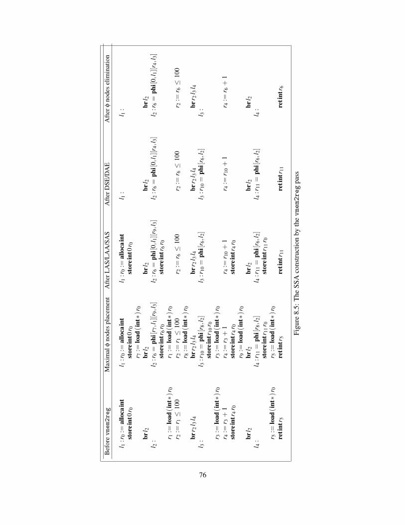
Bef
orevmem2reg
Max
imal
φno
des
plac
emen
tA
fter
LA
S/L
AA
/SA
SA
fter
DSE
/DA
EA
fter
φno
des
elim
inat
ion
l 1:r
0:=
allo
cain
tst
orei
nt0
r 0
brl 2
l 2: r 1
:=lo
ad(i
nt∗)
r 0r 2
:=r 1≤
100
brr 2
l 3l 4
l 3: r 3
:=lo
ad(i
nt∗)
r 0r 4
:=r 3
+1
stor
eint
r 4r 0
brl 2
l 4: r 5
:=lo
ad(i
nt∗)
r 0re
tint
r 5
l 1:r
0:=
allo
cain
tst
orei
nt0
r 0r 7
:=lo
ad(i
nt∗)
r 0br
l 2l 2
:r6=
phi[
r 7,l
1][r
9,l 3]
stor
eint
r 6r 0
r 1:=
load
(int∗)
r 0r 2
:=r 1≤
100
r 8:=
load
(int∗)
r 0br
r 2l 3
l 4l 3
:r10
=ph
i[r 8,l
2]st
orei
ntr 1
0r 0
r 3:=
load
(int∗)
r 0r 4
:=r 3
+1
stor
eint
r 4r 0
r 9:=
load
(int∗)
r 0br
l 2l 4
:r11
=ph
i[r 8,l
2]st
orei
ntr 1
1r 0
r 5:=
load
(int∗)
r 0re
tint
r 5
l 1:r
0:=
allo
cain
tst
orei
nt0
r 0
brl 2
l 2:r
6=
phi[
0,l 1][
r 9,l
3]st
orei
ntr 6
r 0
r 2:=
r 6≤
100
brr 2
l 3l 4
l 3:r
10=
phi[
r 6,l
2]
r 4:=
r 10+
1st
orei
ntr 4
r 0
brl 2
l 4:r
11=
phi[
r 6,l
2]st
orei
ntr 1
1r 0
reti
ntr 1
1
l 1: br
l 2l 2
:r6=
phi[
0,l 1][
r 4,l
3]
r 2:=
r 6≤
100
brr 2
l 3l 4
l 3:r
10=
phi[
r 6,l
2]
r 4:=
r 10+
1
brl 2
l 4:r
11=
phi[
r 6,l
2]
reti
ntr 1
1
l 1: br
l 2l 2
:r6=
phi[
0,l 1][
r 4,l
3]
r 2:=
r 6≤
100
brr 2
l 3l 4
l 3: r 4
:=r 6
+1
brl 2
l 4: re
tint
r 6
Figu
re8.
5:T
heSS
Aco
nstr
uctio
nby
thevmem2reg
pass
76
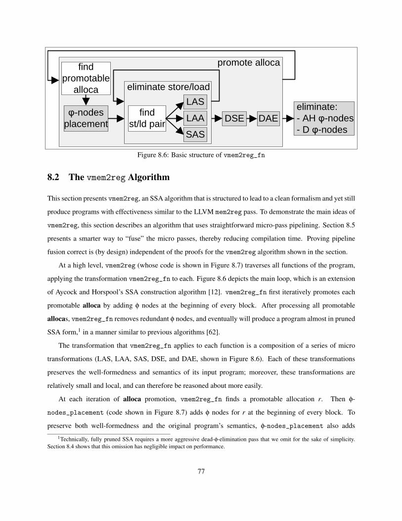
promote alloca
eliminate store/load
LAAφ-nodes
placementDAEDSE
eliminate:
- AH φ-nodes
- D φ-nodes
LAS
SAS
find
promotable
alloca
find
st/ld pair
Figure 8.6: Basic structure of vmem2reg_fn
8.2 The vmem2reg Algorithm
This section presents vmem2reg, an SSA algorithm that is structured to lead to a clean formalism and yet still
produce programs with effectiveness similar to the LLVM mem2reg pass. To demonstrate the main ideas of
vmem2reg, this section describes an algorithm that uses straightforward micro-pass pipelining. Section 8.5
presents a smarter way to “fuse” the micro passes, thereby reducing compilation time. Proving pipeline
fusion correct is (by design) independent of the proofs for the vmem2reg algorithm shown in the section.
At a high level, vmem2reg (whose code is shown in Figure 8.7) traverses all functions of the program,
applying the transformation vmem2reg_fn to each. Figure 8.6 depicts the main loop, which is an extension
of Aycock and Horspool’s SSA construction algorithm [12]. vmem2reg_fn first iteratively promotes each
promotable alloca by adding φ nodes at the beginning of every block. After processing all promotable
allocas, vmem2reg_fn removes redundant φ nodes, and eventually will produce a program almost in pruned
SSA form,1 in a manner similar to previous algorithms [62].
The transformation that vmem2reg_fn applies to each function is a composition of a series of micro
transformations (LAS, LAA, SAS, DSE, and DAE, shown in Figure 8.6). Each of these transformations
preserves the well-formedness and semantics of its input program; moreover, these transformations are
relatively small and local, and can therefore be reasoned about more easily.
At each iteration of alloca promotion, vmem2reg_fn finds a promotable allocation r. Then φ-
nodes_placement (code shown in Figure 8.7) adds φ nodes for r at the beginning of every block. To
preserve both well-formedness and the original program’s semantics, φ-nodes_placement also adds
1Technically, fully pruned SSA requires a more aggressive dead-φ-elimination pass that we omit for the sake of simplicity.Section 8.4 shows that this omission has negligible impact on performance.
77
additional loads and stores around each inserted φ node. At the end of every block that has successors,
φ-nodes_placement introduces a load from r, and stores the result in a fresh temporary; at the beginning
of every block that has predecessor, φ-nodes_placement first inserts a fresh φ node whose incoming value
from a predecessor l is the value of the additional load we added at the end of l, then inserts a store to r
with the value of the inserted φ node.
The second column in Figure 8.5 shows the result of running the φ-node placement pass starting from the
example program in its trivial SSA form. It is not difficult to check that this code is in SSA form. Moreover,
the output program also preserves the meaning of the original program. For example, at the end of block l1,
the program loads the value stored at r0 into r7. After jumping to block l2, the value of r7 is stored into the
location r0, which should contain the same values as r7. Therefore, the additional store does not change the
status of memory. Although the output program contains more temporaries than the original program, these
temporaries are used only to connect inserted loads and stores, and so they do not interfere with the original
temporaries.
To remove the additional loads and stores introduced by the φ-node placement pass and eventually
promote allocas to registers, vmem2reg_fn next applies a series of micro program transformations until no
more optimizations can be applied.
First, vmem2reg_fn iteratively does the following transformations (implemented by eliminate_stld
shown in Figure 8.7):
1. LAS (r1, pc2, val2) “Load After Store”: r1 is loaded from r after a store of val2 to r at program counter
pc2, and there are no other stores of r in any path (on the control-flow graph) from pc2 to r1. In this
case, all uses of r2 can be replaced by val2, and the load can be removed.
2. LAA r1 “Load After Alloca”: As above, but the load is from an uninitialized memory location at r. r1
can be replaced by LLVM’s default memory value, and the load can be removed.
3. SAS (pc1, pc2): The store at program counter pc2 is a store after the store at program counter pc1. If
both of them access r, and there is no load of r in any path (on the control-flow graph) from pc1 to
pc2, then the store at pc1 can be removed.
At each iteration step of eliminate_stld, the algorithm uses the function find_stld_pair to identify
each of the above cases. Because the φ-node placement pass only adds a store and a load as the first and the
last commands at each block respectively, find_stld_pair only needs to search for the above cases within
78
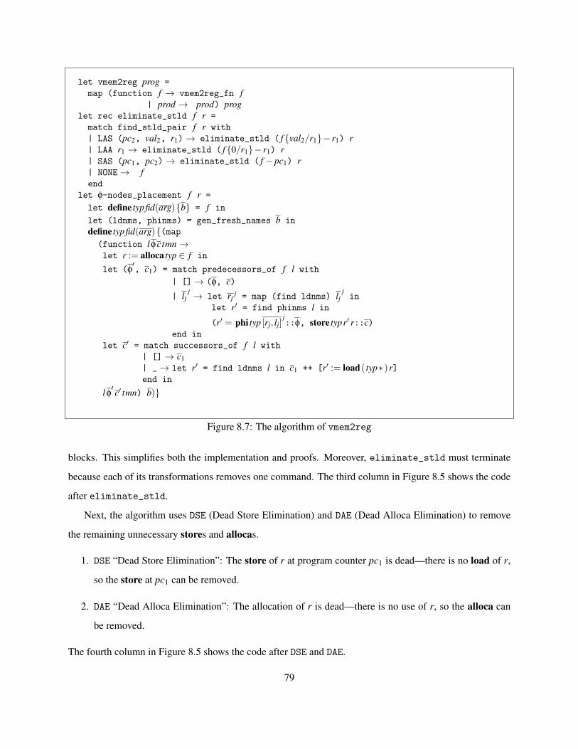
let vmem2reg prog =
map (function f → vmem2reg_fn f| prod → prod) prog
let rec eliminate_stld f r =
match find_stld_pair f r with
| LAS (pc2, val2, r1)→ eliminate_stld ( f{val2/r1}− r1) r| LAA r1 → eliminate_stld ( f{0/r1}− r1) r| SAS (pc1, pc2)→ eliminate_stld ( f −pc1) r| NONE→ fend
let φ-nodes_placement f r =
let define typfid(arg){b} = f in
let (ldnms, phinms) = gen_fresh_names b in
define typfid(arg){(map(function lφctmn→let r := alloca typ ∈ f in
let (φ′, c1) = match predecessors_of f l with
| []→ (φ, c)
| ljj → let rj
j = map (find ldnms) ljjin
let r′ = find phinms l in
(r′ = phi typ [rj, lj]j::φ, store typr′ r::c)
end in
let c′ = match successors_of f l with
| []→ c1| _→ let r′ = find ldnms l in c1 ++ [r′ := load( typ∗)r]end in
lφ′ c′ tmn) b)}
Figure 8.7: The algorithm of vmem2reg
blocks. This simplifies both the implementation and proofs. Moreover, eliminate_stld must terminate
because each of its transformations removes one command. The third column in Figure 8.5 shows the code
after eliminate_stld.
Next, the algorithm uses DSE (Dead Store Elimination) and DAE (Dead Alloca Elimination) to remove
the remaining unnecessary stores and allocas.
1. DSE “Dead Store Elimination”: The store of r at program counter pc1 is dead—there is no load of r,
so the store at pc1 can be removed.
2. DAE “Dead Alloca Elimination”: The allocation of r is dead—there is no use of r, so the alloca can
be removed.
The fourth column in Figure 8.5 shows the code after DSE and DAE.
79
Finally, vmem2reg_fn eliminates unnecessary and dead φ nodes [12]:
1. AH φ-nodes [12]: if any φ is of the form r = phi typ [valj, lj]jwhere all valj are either equal to r or val,
then all uses of r can be replaced by val, and the φ can be removed. Aycock and Horspool [12] proved
that when there is no such φ node in a reducible program, the program is of the minimal SSA form.
2. D φ-nodes: if there is no any use of the φ node. Removing D φ-nodes produces programs in nearly
pruned SSA form.
The right-most column in Figure 8.5 shows the final output of the algorithm.
8.3 Correctness of vmem2reg
We prove the correctness of vmem2reg using the techniques developed in Chapter 5. At a high level, the
correctness of vmem2reg is the composition of the correctness of each micro transformation of vmem2reg
shown in Figure 8.7. Given a well-formed input program, each shaded box must produce a well-formed
program that preserves the semantics of the input program. Moreover, the micro transformations except DAE
and φ-nodes elimination must preserve the promotable predicate (Definition 7), because the correctness of
subsequent transformations relies on fact that promotable allocations aren’t aliased.
Formally, let prog{ f ′/ f} be the substitution of f by f ′ in prog, and let L f M be a micro transformation of
f applied by vmem2reg. L M must satisfy:
1. Preserving promotable: when L M is not DAE or φ-nodes elimination, if promotable( f ,r), then
promotable(L f M,r).
2. Preserving well-formedness: if promotable( f ,r) when L M is φ-nodes placement, and ` prog, then
` prog{L f M/ f}.
3. Program refinement: if promotable( f ,r) when L M is not φ-nodes elimination, and ` prog, then
prog⊇ prog{L f M/ f}.
8.3.1 Preserving promotability
At the beginning of each iteration for promoting allocas, the algorithm indeed finds promotable allocations.
Lemma 25. If prog ` f , and vmem2reg_fn finds a promotable allocation r in f , then promotable( f ,r).
80
We next show that φ-nodes placement preserves promotable:
Lemma 26. If promotable( f ,r),
then promotable(φ–nodes placement f r,r).
Proof (sketch): The φ-nodes placement pass only inserts instructions. Therefore, if r is in the entry block
of the original function, r is still in the entry block of the transformed one. Moreover, in the transformed
function, the instructions copied from the original function use r in the same way, the inserted stores
only write fresh definitions into memory, and the φ-nodes only use fresh definitions. Therefore, r is still
promotable after φ-nodes placement.
Each of the other micro transformations is composed of one or two more basic transformations: variable
substitution, denoted by f{val/r}, and instruction removal, denoted by filtercheck f where filter removes
an instruction insn from f if check insn = false. For example, f{val2/r1} − r1 (LAS) is a substitution
followed by a removal in which check insn = false iff insn defines r1; DSE of a promotable alloca r is a
removal in which check insn = false iff insn is a store to r. We first establish that substitution and removal
preserve promotable.
Lemma 27. Suppose promotable( f ,r),
1. If ¬(val1 usesr), then promotable( f{val1/r1},r).
2. If check insn = false⇒ insn does not define r, then promotable(filtercheck f ,r).
We can show that the other micro transformations preserve promotable by checking the preconditions
of Lemma 27.
Lemma 28. Suppose promotable( f ,r), r is still promotable after LAS, LAA, SAS or DSE.
The substituted value of LAS is written to memory by a store in f , which cannot use r because r is
promotable in f . The substituted value of LAA is a constant that cannot use r trivially. Moreover, LAS, LAA,
SAS and DSE remove only loads or stores.
8.3.2 Preserving well-formedness
It is sufficient to check the following conditions to show that a function-level transformation preserves well-
formedness:
81
Lemma 29. Suppose
1. L f M and f have the same signature.
2. if prog ` f , then prog{L f M/ f} ` L f M.
If ` prog, then ` prog{L f M/ f}.
It is easy to see that all transformations vmem2reg applies satisfy the first condition. We first prove that
φ-nodes placement preserves the second condition:
Lemma 30. If promotable( f ,r), prog ` f and let f ′ be φ–nodes placement f r, then prog{ f ′/ f} ` f ′.
Proof (sketch): Because φ-nodes placement only inserts fresh definitions, and does not change control-
flow graphs, dominance relations are preserved, and all the instructions from the original program are still
well-formed after the transformation.
To show the well-formedness of the inserted instructions, we need to check that they satisfy the use/def
properties of SSA. The inserted instructions only use r or fresh definitions introduced by the pass. The
well-formedness of f ensures that 1) because r is defined at the entry block, it must dominate the end of
all blocks, and the beginning of all non-entry block; 2) the entry block has not predecessors. Therefore, the
definition of r must strictly dominate all its uses in the inserted load’s and store’s. The fresh variable used
by each inserted store is well-formed because its definition is by an inserted φ-node in the same block of
the store, and must strictly dominate its use in the store. The incoming variables used by each φ-node is
well-formed because they are all defined at the end of the corresponding incoming blocks.
Similarly, to reason about other transformations, we first establish that substitution and removal preserve
well-formedness.
Lemma 31. Suppose prog ` f ,
1. If f ` val1� r2, f ′ = f{val1/r2}, then prog{ f ′/ f} ` f ′.
2. If check insn = false⇒ f does not use insn, and let f ′ be filtercheck f , then prog{ f ′/ f} ` f ′.
Here, f ` val1� r2 if f ` r1� r2 when val1 usesr1. Note that the first part of Lemma 31 is an extension
of Lemma 15 that only allows substitution on commands. In vmem2reg, LAS and φ-nodes elimination may
transform φ-nodes.
82

LAS, LAA and φ-nodes elimination remove instructions after substitution. The following auxiliary lemma
shows that the substituted definition is removable after substitution:
Lemma 32. If f ` val1� r2, then f{val1/r2} does not use r2.
This lemma holds because val1 cannot use r2 by Lemma 7.
Lemma 33. LAS, LAA, SAS, DSE, DAE and φ-nodes elimination preserve well-formedness.
Proof (sketch): Most of the proofs follow Lemma 31 and Lemma 32. The interesting case is showing that
if a φ-node in f is of the form r = phi typ [valj, lj]jwhere all valj are either equal to r or val′ (which is an AH
φ-node [12]), then f ` val′� r.
It is trivial if val′ is a constant. Suppose val′usesr′, r and r′ are defined in l and l′ respectively. We first
have that r = phi typ [rj, l]jis not well-formed. Suppose such a φ-node is well-formed. The well-formedness
of the φ-node ensures that the definition of rj dominates the end of all l’s predecessors. Therefore, l strictly
dominates itself. This is a contradiction by Lemma 7.
By the above result, r′ cannot be r, and l′ cannot be l. Suppose ¬ f ` r′ � r. There must exist a
simple path (which has no cycles) from the entry to l that bypasses l′. The simple path must visit one of
l’s predecessors. The predecessor can be neither the one for r because the path is simple, nor the one for r′
because the path bypasses l′. This is a contradiction.
8.3.3 Program refinement
The proofs of program refinement use the simulation diagrams in Chapter 2 and different instantiations of
the GWF FR rule we developed in Chapter 5, where instead of just a function f and frame σ, we now have
a configuration config that also includes the program memory.
config,P ` S , S ∈ config.prog∧Pconfig(S|sdom)
Let σ|sdom be (σ. f , σ.pc, (σ.δ)|(sdom(σ. f )(σ.pc)), σ.α). S|sdom is (S.M,S.σ|sdom). S ∈ prog ensures that all f
and pc in each frame of S are defined in prog.
Promotability As we discussed above, the micro transformations (except φ-nodes elimination) rely on
the promotable property. We start by establishing the invariants related to promotability, namely that
promotable allocations aren’t aliased. This proof is itself an application of GWF FR.
83
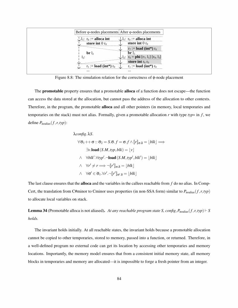
l1: r0 := alloca int store int 0 r0
br l2
store int r6 r0
r1 := load (int*) r0
r7 := load (int*) r0
...
l1: r0 := alloca int
store int 0 r0
r1 := load (int*) r0
...
l2:
Before φ-nodes placements After φ-nodes placements
br l2
r6 = phi [r7, l1] [r9, l3]l2:
Figure 8.8: The simulation relation for the correctness of φ-node placement
The promotable property ensures that a promotable alloca of a function does not escape—the function
can access the data stored at the allocation, but cannot pass the address of the allocation to other contexts.
Therefore, in the program, the promotable alloca and all other pointers (in memory, local temporaries and
temporaries on the stack) must not alias. Formally, given a promotable allocation r with type typ∗ in f , we
define Pnoalias( f ,r, typ):
λconfig.λS.
∀σ1++σ :: σ2 = S.σ. f = σ. f ∧ JrKσ.δ = bblkc=⇒
∃v.load(S.M, typ,blk) = bvc
∧ ∀blk′.∀typ′.¬load(S.M, typ′,blk′) = bblkc
∧ ∀r′ 6= r =⇒¬Jr′Kσ.δ = bblkc
∧ ∀σ′ ∈ σ1.∀r′.¬Jr′Kσ′.δ = bblkc
The last clause ensures that the alloca and the variables in the callees reachable from f do no alias. In Comp-
Cert, the translation from C#minor to Cminor uses properties (in non-SSA form) similar to Pnoalias( f ,r, typ)
to allocate local variables on stack.
Lemma 34 (Promotable alloca is not aliased). At any reachable program state S, config,Pnoalias( f ,r, typ)` S
holds.
The invariant holds initially. At all reachable states, the invariant holds because a promotable allocation
cannot be copied to other temporaries, stored to memory, passed into a function, or returned. Therefore, in
a well-defined program no external code can get its location by accessing other temporaries and memory
locations. Importantly, the memory model ensures that from a consistent initial memory state, all memory
blocks in temporaries and memory are allocated—it is impossible to forge a fresh pointer from an integer.
84

φ-node placement Figure 8.8 pictorially shows an example (which is the code fragment from Figure 8.5)
of the simulation relation ∼ for proving that the φ-node placement preserves semantics. It follows left
“option” simulation, because φ-node placement only inserts instructions. We use the number of unexecuted
instructions in the current block as the measure function.
The dashed lines indicate where the two program counters must be synchronized. Although the pass
defines new variables and stores (shaded in Figure 8.8), the variables are only passed to the new φ nodes,
or stored into the promotable allocation; additional stores only update the promotable allocation with the
same value. Therefore, by Lemma 34, ∼ requires that two programs have the same memory states and the
original temporaries match.
Lemma 35.
If f ′ = φ–nodes placement f r, and promotable( f ,r), and ` prog, then prog⊇ prog{ f ′/ f}.
The interesting case is to show that ∼ implies a correspondence between stuck states. Lemma 34
ensures that the promotable allocation cannot be dereferenced by operations on other pointers. Therefore,
the inserted memory accesses are always safe.
LAS/LAA We present the proofs for the correctness of LAS. The proofs for the correctness of LAA is similar.
In the code after φ-node placement of Figure 8.5, r7 := load( int∗)r0 is an LAS of store int0r0. We observe
that at any program counter pc between the store and load, the value stored at r0 must be 0 because
alive(pc1,pc2) holds—the store defined at pc1 is not overwritten by other writes until pc.
To formalize the observation, consider a promotable r with type typ∗ in f . Suppose find_stld_pair
f r = LAS (pc2, val2, r1). Consider the invariant Plas( f ,r, typ,pc2,val2):
λconfig.λS.∀σ ∈ S.σ.
( f = σ. f ∧ Jval2Kσ.δ = bv2c∧ JrKσ.δ = bblkc∧
alive(pc2,σ.pc)) =⇒ load(S.M, typ,blk) = bv2c
Using Lemma 34, we have that:
Lemma 36. If promotable( f ,r), then alive(pc2,r1) and at any reachable state S, config,Plas( f ,r, typ,pc2,val2)`
S holds.
85
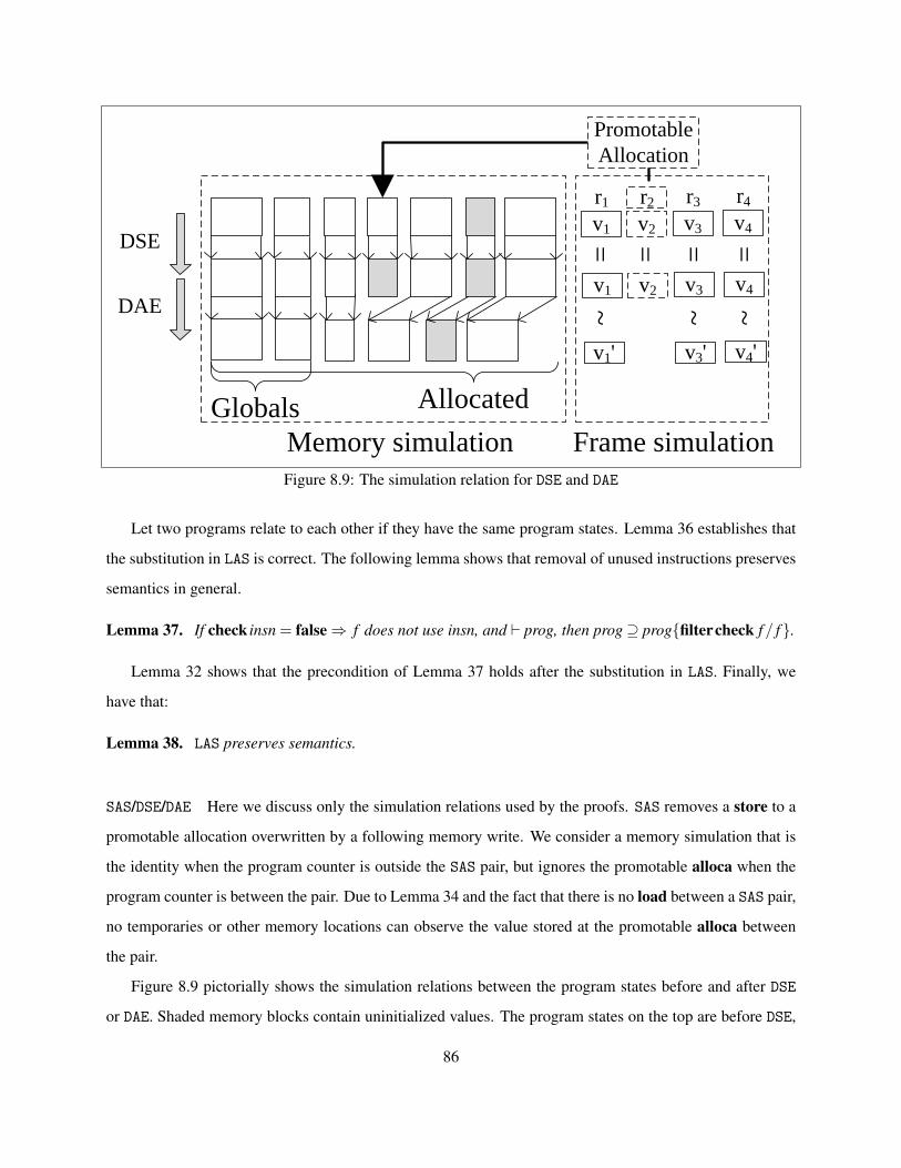
Globals Allocated
v1 v2 v3 v4
Memory simulation Frame simulation
v1 v2 v3 v4
v1' v3' v4'
Promotable
Allocation
DSE
DAE
r1 r2 r3 r4
~ ~ ~
= = = =
Figure 8.9: The simulation relation for DSE and DAE
Let two programs relate to each other if they have the same program states. Lemma 36 establishes that
the substitution in LAS is correct. The following lemma shows that removal of unused instructions preserves
semantics in general.
Lemma 37. If check insn = false⇒ f does not use insn, and ` prog, then prog⊇ prog{filtercheck f/ f}.
Lemma 32 shows that the precondition of Lemma 37 holds after the substitution in LAS. Finally, we
have that:
Lemma 38. LAS preserves semantics.
SAS/DSE/DAE Here we discuss only the simulation relations used by the proofs. SAS removes a store to a
promotable allocation overwritten by a following memory write. We consider a memory simulation that is
the identity when the program counter is outside the SAS pair, but ignores the promotable alloca when the
program counter is between the pair. Due to Lemma 34 and the fact that there is no load between a SAS pair,
no temporaries or other memory locations can observe the value stored at the promotable alloca between
the pair.
Figure 8.9 pictorially shows the simulation relations between the program states before and after DSE
or DAE. Shaded memory blocks contain uninitialized values. The program states on the top are before DSE,
86
where r2 is a temporary that holds the promotable stack allocation and is not used by any loads. After
DSE, the memory values for the promotable allocation may not match the original program’s corresponding
block. However, values in temporaries and all other memory locations must be unchanged (by Lemma 34).
Note that unmatched memory states only occur after the promotable allocation; before the allocation, the
two memory states should be the same.
The bottom part of Figure 8.9 illustrates the relations between programs before and after DAE. After
DAE, the correspondence between memory blocks of the two programs is not bijective, due to the removal of
the promotable alloca. However, there must exist a mapping ∼ from the output program’s memory blocks
to the original program’s memory blocks. The simulation requires that all values stored in memory and
temporaries (except the promotable allocation) are equal modulo the mapping ∼.
φ-nodes elimination Consider r = phi typ [valj, lj]j
(an AH φ-node) where all the valj’s are either equal
to r or some val′. Lemma 33 showed that f ` val′� r. Intuitively, at any pc that both val′ and r strictly
dominate, the values of val′ and r must be the same. Consider the invariant Pah( f ,r,val′):
λconfig.λS.∀σ ∈ S.σ.
f = σ. f ∧ JrKσ.δ = bv1c∧ Jval′Kσ.δ = bv2c=⇒ v1 = v2
Lemma 39. config,Pah( f ,r,val′) ` S holds for any reachable program state S.
Lemma 39 establishes that the substitution in φ-nodes elimination is correct by using the identity relation.
Lemma 32 and Lemma 37 show that removing dead φ-nodes is correct.
8.3.4 The correctness of vmem2reg
Our main result, fully verified in Coq, is the composition of the correctness proofs for all the micro program
transformations:
Theorem 40 (vmem2reg is correct). If f ′ = vmem2reg f and ` prog, then ` prog{ f ′/ f} and prog ⊇
prog{ f ′/ f}.
87
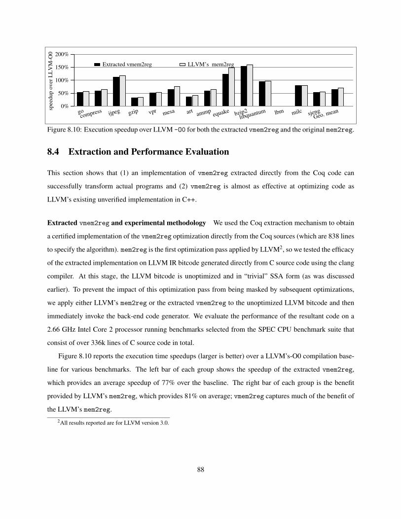
0%
50%
100%
150%
200%sp
eedup o
ver
LL
VM
-O0
Extracted vmem2reg LLVM’s mem2reg
gocompress ijpeg gzip vpr mesa art
ammpequake
bzip2libquantum lbm milc sjeng
Geo. mean
Figure 8.10: Execution speedup over LLVM -O0 for both the extracted vmem2reg and the original mem2reg.
8.4 Extraction and Performance Evaluation
This section shows that (1) an implementation of vmem2reg extracted directly from the Coq code can
successfully transform actual programs and (2) vmem2reg is almost as effective at optimizing code as
LLVM’s existing unverified implementation in C++.
Extracted vmem2reg and experimental methodology We used the Coq extraction mechanism to obtain
a certified implementation of the vmem2reg optimization directly from the Coq sources (which are 838 lines
to specify the algorithm). mem2reg is the first optimization pass applied by LLVM2, so we tested the efficacy
of the extracted implementation on LLVM IR bitcode generated directly from C source code using the clang
compiler. At this stage, the LLVM bitcode is unoptimized and in “trivial” SSA form (as was discussed
earlier). To prevent the impact of this optimization pass from being masked by subsequent optimizations,
we apply either LLVM’s mem2reg or the extracted vmem2reg to the unoptimized LLVM bitcode and then
immediately invoke the back-end code generator. We evaluate the performance of the resultant code on a
2.66 GHz Intel Core 2 processor running benchmarks selected from the SPEC CPU benchmark suite that
consist of over 336k lines of C source code in total.
Figure 8.10 reports the execution time speedups (larger is better) over a LLVM’s-O0 compilation base-
line for various benchmarks. The left bar of each group shows the speedup of the extracted vmem2reg,
which provides an average speedup of 77% over the baseline. The right bar of each group is the benefit
provided by LLVM’s mem2reg, which provides 81% on average; vmem2reg captures much of the benefit of
the LLVM’s mem2reg.
2All results reported are for LLVM version 3.0.
88

0
1
10
100
1000
10000
com
pila
tion
over
head
ove
r m
em2r
eg Imperative vmem2reg-O2 Extracted vmem2reg
Extracted vmem2reg-O1 Extracted vmem2reg-O2
gocompress ijpeg gzip vpr
mesa artammp
equakebzip2
parsertwolf bzip2 mcf
hmmer
libquantum lbm milc sjengh264ref
Geo. mean
Figure 8.11: Compilation overhead over LLVM’s original mem2reg.
Comparing vmem2reg and mem2reg The vmem2reg pass differs from LLVM’s mem2reg in a few ways.
First, mem2reg promotes allocas used by LLVM’s intrinsics, while vmem2reg conservatively considers such
allocas to potentially escape, and so does not promote them. We determined that such intrinsics (used by
LLVM to annotate the liveness of variable definitions) lead to almost all the difference in performance in
the equake benchmark. Second, although vmem2reg deletes most unused φ-nodes, it does not aggressively
remove them and, therefore, does not generate fully pruned SSA as mem2reg does. However, our results
show that this does not impose a significant difference in performance.
8.5 Optimized vmem2reg
The algorithm of vmem2reg is designed with verification in mind, but it is not efficient in practice: Fig-
ure 8.11 shows that on average vmem2reg is 329 times slower than mem2reg in terms of compile-time. Such
an inefficient design is aimed at streamlining the presentation of the proof techniques we developed for SSA,
such that our research can focus on the crucial part of the problem—understanding how the proofs should
go. This section shows how to design an efficient algorithm based on vmem2reg, and verify its correctness
by extending the proofs for vmem2reg.
The costs of vmem2reg include (1) the pessimistic φ-node insertion algorithm, which introduces unnec-
essary φ nodes that lead to more inserted loads and stores to remove; and (2) the pipelined strategy that
requires much more passes than necessary. Given a CFG with N nodes and I instructions and a promotable
alloca, vmem2reg, in the worst case, first inserts N φ nodes and N “Load After Store” or “Load After Alloca”
89

promote alloca
eliminate store/load
via block lists
φ-nodes
placementDAEDSE
eliminate:
- AH φ-nodes
- D φ-nodes
find
promotable
alloca
lookup composesubstitute
delete
Figure 8.12: Basic structure of vmem2reg-O1
pairs, then takes N passes to promote the loads and stores, and finally takes at most N passes to remove AH
φ-nodes. Therefore, the complexity of vmem2reg is O(N ∗ I).
To address the compilation overhead, we implemented two improved algorithms: vmem2reg-O1
and vmem2reg-O2 in terms of the difficulty for reasoning about their correctness. Section 8.5.1 shows
vmem2reg-O1 that composes the pipelined elimination passes into a single pass. Section 8.5.2 shows
vmem2reg-O2 that improves vmem2reg-O1 by placing the minimal number of φ nodes at domination
frontier, and does not need the AH φ-node elimination pass. Note that vmem2reg-O1 is verified in Coq, and
vmem2reg-O2 is not fully verified in Coq.
8.5.1 O1 Level—Pipeline fusion
Figure 8.12 gives the structure of vmem2reg-O1, which takes one pass to collect all LAS/LAA pairs and
then uses one more pass to remove them. Figure 8.13 presents the composed elimination algorithm
(eliminate_stld). We denote each micro elimination by actions ac.
Actions ac : : = r 7→ val Lists of Actions AC : : = /0 | ac,AC
Here, r 7→ val denotes LAS (r, pc, val) or LAA r with the default memory value val. Note that unlike
vmem2reg the optimized version does not consider SAS because (1) the later DSE removes all dead stores in
one pass (2) vmem2reg-O2 (in Section 8.5.2) needs to traverse all subtrees to find SAS, which does not lead
to a simple algorithm.
To find all initial elimination pairs AC, eliminate_stld traverses the list of blocks of a function, finds
elimination pairs for each block (by find_stld_pairs_block), and then concatenates them. At each
block, we use stld_state to keep track of the search state (by find_stld_pairs_cmd): STLD_INIT is
the initial state; STLD_AL typ records the element type of the memory value stored at the latest promotable
90
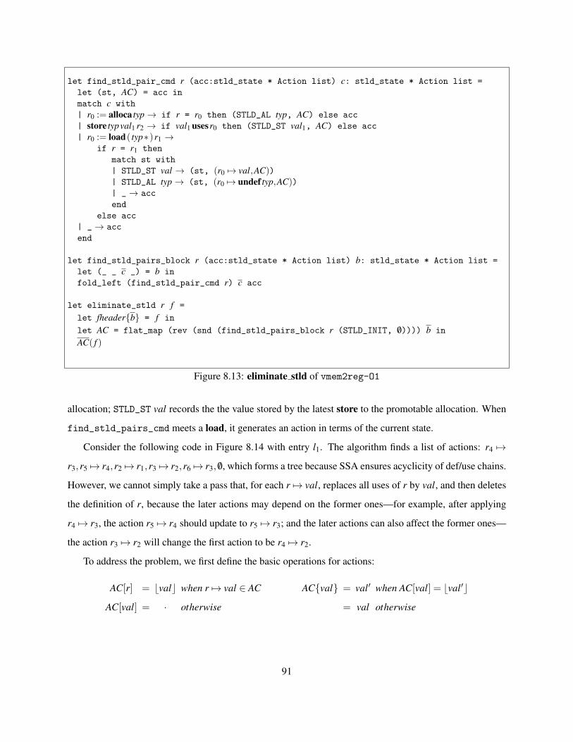
let find_stld_pair_cmd r (acc:stld_state * Action list) c: stld_state * Action list =
let (st, AC) = acc in
match c with
| r0 := alloca typ→ if r = r0 then (STLD_AL typ, AC) else acc
| store typval1 r2 → if val1 usesr0 then (STLD_ST val1, AC) else acc
| r0 := load( typ∗)r1 →if r = r1 then
match st with
| STLD_ST val → (st, (r0 7→ val,AC))| STLD_AL typ→ (st, (r0 7→ undef typ,AC))| _→ acc
end
else acc
| _→ acc
end
let find_stld_pairs_block r (acc:stld_state * Action list) b: stld_state * Action list =
let (_ _ c _) = b in
fold_left (find_stld_pair_cmd r) c acc
let eliminate_stld r f =
let fheader{b} = f in
let AC = flat_map (rev (snd (find_stld_pairs_block r (STLD_INIT, /0)))) b in
AC( f )
Figure 8.13: eliminate stld of vmem2reg-O1
allocation; STLD_ST val records the the value stored by the latest store to the promotable allocation. When
find_stld_pairs_cmd meets a load, it generates an action in terms of the current state.
Consider the following code in Figure 8.14 with entry l1. The algorithm finds a list of actions: r4 7→
r3,r5 7→ r4,r2 7→ r1,r3 7→ r2,r6 7→ r3, /0, which forms a tree because SSA ensures acyclicity of def/use chains.
However, we cannot simply take a pass that, for each r 7→ val, replaces all uses of r by val, and then deletes
the definition of r, because the later actions may depend on the former ones—for example, after applying
r4 7→ r3, the action r5 7→ r4 should update to r5 7→ r3; and the later actions can also affect the former ones—
the action r3 7→ r2 will change the first action to be r4 7→ r2.
To address the problem, we first define the basic operations for actions:
AC[r] = bvalc when r 7→ val ∈ AC AC{val} = val′ when AC[val] = bval′c
AC[val] = · otherwise = val otherwise
91
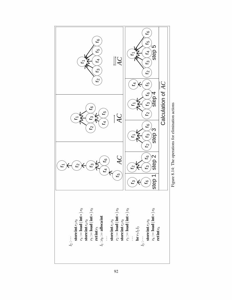
l 2:··· stor
eint
r 3r 0
r 4:=
load
(int∗)
r 0st
orei
ntr 4
r 0r 5
:=lo
ad(i
nt∗)
r 0re
tint
r 5l 1
:r0
:=al
loca
int
···
stor
eint
r 1r 0
r 2:=
load
(int∗)
r 0st
orei
ntr 2
r 0r 3
:=lo
ad(i
nt∗)
r 0···
brr 7
l 2l 3
l 3:··· stor
eint
r 3r 0
r 6:=
load
(int∗)
r 0re
tint
r 6
r 3 r 6r 3r 2
r 6r 3r 1
r 6r 2
r 3r 1
r 6r 2
r 4 r 5
r 1
r 3r 2
r 4r 6
r 5ste
p 1
ste
p 2
ste
p 3
ste
p 4
ste
p 5
r 1
r 3r 2
r 4r 6
r 5
r 1 r 3r 2
r 4
r 6
r 5
r 1 r 3r 2
r 4r 6
r 5A
CA
CA
C
AC
Ca
lcu
latio
n o
f
Figu
re8.
14:T
heop
erat
ions
fore
limin
atio
nac
tions
92
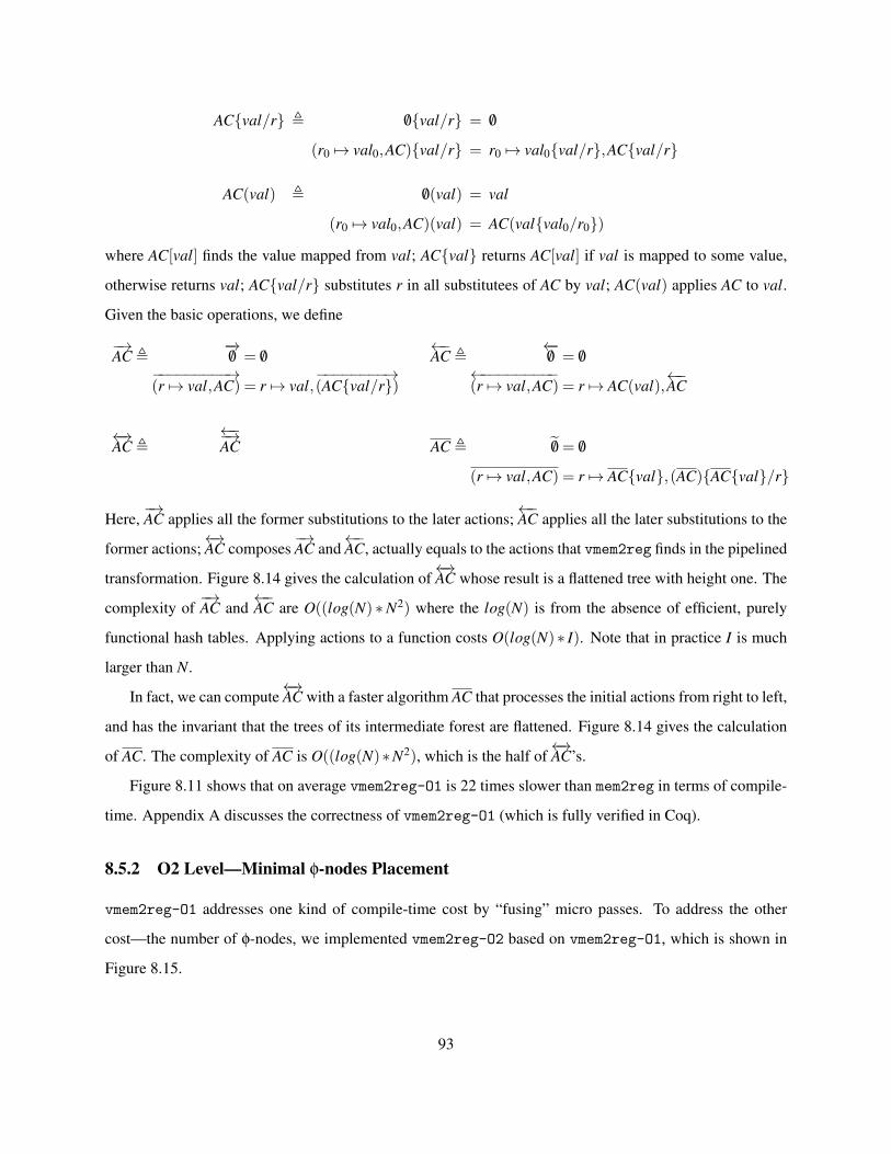
AC{val/r} , /0{val/r} = /0
(r0 7→ val0,AC){val/r} = r0 7→ val0{val/r},AC{val/r}
AC(val) , /0(val) = val
(r0 7→ val0,AC)(val) = AC(val{val0/r0})
where AC[val] finds the value mapped from val; AC{val} returns AC[val] if val is mapped to some value,
otherwise returns val; AC{val/r} substitutes r in all substitutees of AC by val; AC(val) applies AC to val.
Given the basic operations, we define
−→AC ,
−→/0 = /0
←−AC ,
←−/0 = /0
−−−−−−−−−→(r 7→ val,AC) = r 7→ val,
−−−−−−−−→(AC{val/r})
←−−−−−−−−−(r 7→ val,AC) = r 7→ AC(val),
←−AC
←→AC ,
←−−→AC AC , /0 = /0
(r 7→ val,AC) = r 7→ AC{val},(AC){AC{val}/r}
Here,−→AC applies all the former substitutions to the later actions;
←−AC applies all the later substitutions to the
former actions;←→AC composes
−→AC and
←−AC, actually equals to the actions that vmem2reg finds in the pipelined
transformation. Figure 8.14 gives the calculation of←→AC whose result is a flattened tree with height one. The
complexity of−→AC and
←−AC are O((log(N) ∗N2) where the log(N) is from the absence of efficient, purely
functional hash tables. Applying actions to a function costs O(log(N) ∗ I). Note that in practice I is much
larger than N.
In fact, we can compute←→AC with a faster algorithm AC that processes the initial actions from right to left,
and has the invariant that the trees of its intermediate forest are flattened. Figure 8.14 gives the calculation
of AC. The complexity of AC is O((log(N)∗N2), which is the half of←→AC’s.
Figure 8.11 shows that on average vmem2reg-O1 is 22 times slower than mem2reg in terms of compile-
time. Appendix A discusses the correctness of vmem2reg-O1 (which is fully verified in Coq).
8.5.2 O2 Level—Minimal φ-nodes Placement
vmem2reg-O1 addresses one kind of compile-time cost by “fusing” micro passes. To address the other
cost—the number of φ-nodes, we implemented vmem2reg-O2 based on vmem2reg-O1, which is shown in
Figure 8.15.
93
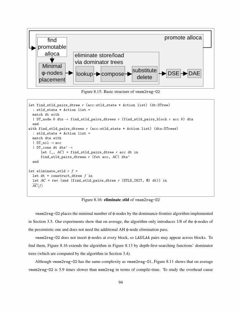
promote alloca
eliminate store/load
via dominator treesMinimal
φ-nodes
placementDAEDSE
find
promotable
alloca
lookup composesubstitute
delete
Figure 8.15: Basic structure of vmem2reg-O2
let find_stld_pairs_dtree r (acc:stld_state * Action list) (dt:DTree)
: stld_state * Action list =
match dt with
| DT_node b dts→ find_stld_pairs_dtrees r (find_stld_pairs_block r acc b) dts
end
with find_stld_pairs_dtrees r (acc:stld_state * Action list) (dts:DTrees)
: stld_state * Action list =
match dts with
| DT_nil→ acc
| DT_cons dt dts’→let (_, AC) = find_stld_pairs_dtree r acc dt in
find_stld_pairs_dtrees r (fst acc, AC) dts’
end
let eliminate_stld r f =
let dt = construct_dtree f in
let AC = rev (snd (find_stld_pairs_dtree r (STLD_INIT, /0) dt)) in
AC( f )
Figure 8.16: eliminate stld of vmem2reg-O2
vmem2reg-O2 places the minimal number of φ-nodes by the dominance-frontier algorithm implemented
in Section 3.5. Our experiments show that on average, the algorithm only introduces 1/8 of the φ-nodes of
the pessimistic one and does not need the additional AH φ-node elimination pass.
vmem2reg-O2 does not insert φ-nodes at every block, so LAS/LAA pairs may appear across blocks. To
find them, Figure 8.16 extends the algorithm in Figure 8.13 by depth-first-searching functions’ dominator
trees (which are computed by the algorithm in Section 3.4).
Although vmem2reg-O2 has the same complexity as vmem2reg-O1, Figure 8.11 shows that on average
vmem2reg-O2 is 5.9 times slower than mem2reg in terms of compile-time. To study the overhead cause
94
by the purely functional programming, we also implemented the C++ version of vmem2reg-O2. Because it
uses constant-time hashtables and does alias-based substitution, the C++ version’s complexity is O(I). In
practice, Figure 8.11 shows that its compile-time is 0.63 time of mem2reg’s because we use a slightly more
efficient dominance-frontier calculation [24] and do not allow intrinsics to use promotable allocations.
The correctness of vmem2reg-O2 is composed of two parts. The first part needs to generalize the proofs
of vmem2reg that assume that LAS/LAA pairs must be in the same block to allow LAS/LAA pairs in terms of
arbitrary domination relations. The second part can reuse the proofs of vmem2reg-O1 for reasoning about
composing micro transformations. Appendix B discusses the correctness of vmem2reg-O2 (which have not
fully been verified in Coq).
95
Chapter 9
The Coq Development
This chapter summarizes our Coq development.
9.1 Definitions
Table 9.1 shows the size of our development. Note that the size of the formalism of vmem2reg-O1 does not
include the development of vmem2reg. Vellvm encodes the abstract syntax from Chapter 6 in an entirely
straightforward way using Coq’s inductive datatypes (generated in a preprocessing step via the Ott [60]
tool). The implementation uses Penn’s Metatheory library [13], which was originally designed for the
locally nameless representation, to represent identifiers of the LLVM, and to reason about their freshness.
The Coq representation deviates from the full LLVM language in only a few (mostly minor) ways. In
particular, the Coq representation requires that some type annotations be in normal form (e.g., the type
annotation on load must be a pointer; named types must be sorted in terms of their dependency), which
simplifies type checking at the IR level. The Vellvm tool that imports LLVM bitcode into Coq provides such
normalization, which simply expands definitions to reach the normal form.
Vellvm’s type system is also represented via Ott [60], and refers to the imperative LLVM verification
pass that checks the well-formedness of LLVM bitcode. The current type system is formalized by predicates
that is not extractable. We leave the extraction as our future work, i.e., a verified LLVM type checker.
Vellvm’s memory model implementation extends CompCert’s with 8,889 lines of code to support inte-
gers with arbitrary precision, padding, and an experimental treatment of casts that has not yet needed for any
96
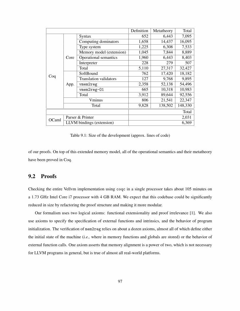
Definition Metatheory Total
Coq
Core
Syntax 652 6,443 7,095Computing dominators 1,658 14,437 16,095Type system 1,225 6,308 7,533Memory model (extension) 1,045 7,844 8,889Operational semantics 1,960 6,443 8,403Interpreter 228 279 507Total 5,110 27,317 32,427
App.
SoftBound 762 17,420 18,182Translation validators 127 9,768 9,895vmem2reg 2,358 52,138 54,496vmem2reg-O1 665 10,318 10,983Total 3,912 89,644 92,556
Vminus 806 21,541 22,347Total 9,828 138,502 148,330
Total
OCamlParser & Printer 2,031LLVM bindings (extension) 6,369
Table 9.1: Size of the development (approx. lines of code)
of our proofs. On top of this extended memory model, all of the operational semantics and their metatheory
have been proved in Coq.
9.2 Proofs
Checking the entire Vellvm implementation using coqc in a single processor takes about 105 minutes on
a 1.73 GHz Intel Core i7 processor with 4 GB RAM. We expect that this codebase could be significantly
reduced in size by refactoring the proof structure and making it more modular.
Our formalism uses two logical axioms: functional extensionality and proof irrelevance [1]. We also
use axioms to specify the specification of external functions and intrinsics, and the behavior of program
initialization. The verification of mem2reg relies on about a dozen axioms, almost all of which define either
the initial state of the machine (i.e., where in memory functions and globals are stored) or the behavior of
external function calls. One axiom asserts that memory alignment is a power of two, which is not necessary
for LLVM programs in general, but is true of almost all real-world platforms.
97

9.3 OCaml Bindings and Coq Extraction
The LLVM distribution includes primitive OCaml bindings that are sufficient to generate LLVM IR code
(“bitcode” in LLVM jargon) from OCaml. To convert between the LLVM bitcode representation and the
extracted OCaml representation, we implemented a library consisting of about 8,400 lines of OCaml-LLVM
bindings. This library also supports pretty-printing of the abstract syntax tree of the LLVM IR; this code
was also useful in the extracted interpreter.
98

Chapter 10
Related Work
Verified compilers Compiler verification has a considerable history; see the bibliography of Leroy [42]
for a comprehensive overview. Vellvm is closest in spirit to CompCert [42], which was the first fully-verified
compiler to generate compact and efficient assembly code for a large fragment of the C language. CompCert
also uses Coq. It formalizes the operational semantics of CompCert C, several intermediate languages
used in the compilation, and assembly languages including PowerPC, ARM and x86. The latest version
of CompCert also provides an executable reference interpreter for the semantics of CompCert C. Based on
the formalized semantics, the CompCert project fully proves that all compiler phases produce programs that
preserve the semantics of the original program. Optimization passes include local value numbering, constant
propagation, coalescing graph coloring register allocation [18], and other back-end transformations. It uses
translation validators for certifying advanced compiler optimizations, such as instruction scheduling [68],
lazy code motion [69], and software pipelining [70]. The XCERT project [64, 66] extends the CompCert
compiler by a generic translation validator based on SMT solvers.
Other research has also used Coq for compiler verification tasks, including much recent work on com-
piling functional source languages to assembly [15, 21, 22].
Formalization for computing dominators The CompCertSSA project [14] improves the CompCert com-
piler by creating a verified SSA-based middle-end and a GVN optimization pass. They also formalize the
AC algorithm to validate SSA construction and GVN passes, and prove the soundness of AC. We implement
both AC and CHK—an extension of AC in a generic way, and prove they are both sound and complete. We
also provide the corresponding dominator tree constructions, and evaluate performance.
99

There are also informal formalizations for computing dominators. Georgiadis and Tarjan [30] propose
an almost linear-time algorithm that validates if a tree is a dominator tree of a CFG. Although the algorithm
is fast, it is nearly as complicated as the LT algorithm, and it requires a substantial amount of graph theory.
Ramalingam [4] proposes another dominator tree validation algorithm by reducing validating dominator
trees to validating loop structures. However, in practice, most of modern loop identification algorithms used
in LLVM and GCC are based on dominance analysis to find loop headers and bodies.
Formalization for SSA and SSA-based optimizations Verifying the correctness of compiler transfor-
mations is an active research area with a sizable amount of literature. We focus on the work relevant to
SSA-based optimizations.
CompCertSSA verified a translation validator for an SSA construction algorithm that takes imperative
variables to variables in a pruned SSA form. In contrast, our work fully verifies the SSA construction pass
vmem2reg for LLVM directly. A bug in the CompCertSSA compiler will cause the validator to abort the
compilation, whereas verifying the compiler rules out such a possibility. More pragmatically, translation
validation is harder to apply in the context of LLVM, because the compiler infrastructure was not created
with validation in mind. For example, the CompCertSSA translations maintain a close mapping between
source and target variable names so that simulation can be checked by simple erasure; this is not feasible in
the LLVM framework. The CompCertSSA project reports performance measurements of only small bench-
marks totaling about 6k lines, whereas we have tested our pass on 336k lines, including larger programs.
Unsurprisingly, the CompCertSSA and Vellvm proofs share some similarities. For example, CompCert-
SSA’s GVN proof uses an invariant similar to the one in our Theorem 13 and Lemma 17. However, the
LLVM’s strategy of promoting allocas means that our proofs need a combination of both SSA and aliasing
properties to prove correctness. Moreover, our proof technique of pipelining “micro” transformations is
novel, and it should be broadly applicable.
To fully prove GVN, we would need additional properties about congruence-based term equivalence.
Although this fits naturally into our framework, Figure 8.2 shows that the combination of GVN with all
other optimizations (except mem2reg) does not provide significant speedup—the full suite of -O2 and -O3
level optimizations only yields a 11% speedup (on average).
The validation algorithm of CompCertSSA is proven to be complete to certificate the classic SSA
construction [28] (which computes dominators by the Lengauer-Tarjan algorithm [40]). Although vmem2reg
is based on the Aycock-Horspool algorithm [12], Section 8.5 shows that the correctness of the classic
100
algorithm is independent to the proofs for vmem2reg, and that the performance of the optimized vmem2reg
is compatible with the classic algorithm.
Mansky et al. designed an Isabelle/HOL framework that uses control-flow graph rewrites to transform
programs and uses temporal logic and model-checking to specify and prove the correctness of program
transformations [45]. They verified an SSA construction algorithm in the framework. Other researchers
have formalized specific SSA-based optimizations by using SSA forms with different styles of semantics:
an informal semantics that describes the intuitive idea of the SSA form [28]; an operational semantics based
on a matrix representation of φ nodes [72]; a data-flow semantics based term graphs using the Isabelle/HOL
proof assistant [19]. Matsuno et al. defined a type system equivalent to the SSA form and proved that dead
code elimination and common subexpression elimination preserve types [47]. There are also conversions
between the programs in SSA form and functional programs [9, 34].
Validating LLVM optimizations The CoVac project [74] develops a methodology that adapts existing
program analysis techniques to the setting of translation validation, and it reports on a prototype tool that
applies their methodology to verification of the LLVM compiler. The LLVM-MD project [67] validates
LLVM optimizations by symbolic evaluation. The Peggy tool performs translation validation for the LLVM
compiler using a technique called equality saturation [63]. These applications are not fully certified.
Mechanized language semantics There is a large literature on formalizing language semantics and rea-
soning about the correctness of language implementations. Prominent examples include: Foundational Proof
Carrying Code [10], Foundational Typed Assembly Language [26], Standard ML [27, 65], and (a substantial
subset of) Java [37].
Other mechanization efforts The verified software tool-chain project [11] assures that the machine-
checked proofs claimed at the top of the tool-chain hold in the machine language program. Typed assembly
languages [20] provide a platform for proving back-end optimizations. Similarly, The Verisoft project [6]
also attempts to mathematically prove the correct functionality of systems in automotive engineering and se-
curity technology. ARMor [78] guarantees control flow integrity for application code running on embedded
processors. The Rhodium project [41] uses a domain specific language to express optimizations via local
rewrite rules and provides a soundness checker for optimizations
101
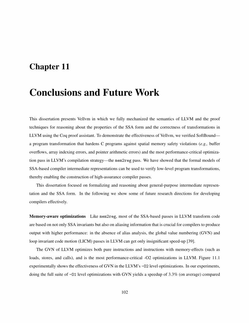
Chapter 11
Conclusions and Future Work
This dissertation presents Vellvm in which we fully mechanized the semantics of LLVM and the proof
techniques for reasoning about the properties of the SSA form and the correctness of transformations in
LLVM using the Coq proof assistant. To demonstrate the effectiveness of Vellvm, we verified SoftBound—
a program transformation that hardens C programs against spatial memory safety violations (e.g., buffer
overflows, array indexing errors, and pointer arithmetic errors) and the most performance-critical optimiza-
tion pass in LLVM’s compilation strategy—the mem2reg pass. We have showed that the formal models of
SSA-based compiler intermediate representations can be used to verify low-level program transformations,
thereby enabling the construction of high-assurance compiler passes.
This dissertation focused on formalizing and reasoning about general-purpose intermediate represen-
tation and the SSA form. In the following we show some of future research directions for developing
compilers effectively.
Memory-aware optimizations Like mem2reg, most of the SSA-based passes in LLVM transform code
are based on not only SSA invariants but also on aliasing information that is crucial for compilers to produce
output with higher performance: in the absence of alias analysis, the global value numbering (GVN) and
loop invariant code motion (LICM) passes in LLVM can get only insignificant speed-up [39].
The GVN of LLVM optimizes both pure instructions and instructions with memory-effects (such as
loads, stores, and calls), and is the most performance-critical -O2 optimizations in LLVM. Figure 11.1
experimentally shows the effectiveness of GVN in the LLVM’s -O2 level optimizations. In our experiments,
doing the full suite of -O1 level optimizations with GVN yields a speedup of 3.3% (on average) compared
102
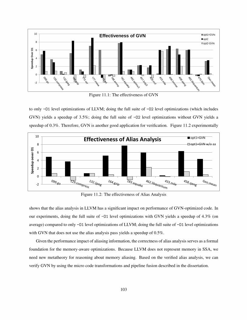
-2
0
2
4
6
8
10 S
peed
up
Ov
er
O1
Effectiveness of GVN opt1+GVN
opt2
opt2-GVN
Figure 11.1: The effectiveness of GVN
to only -O1 level optimizations of LLVM; doing the full suite of -O2 level optimizations (which includes
GVN) yields a speedup of 3.5%; doing the full suite of -O2 level optimizations without GVN yields a
speedup of 0.3%. Therefore, GVN is another good application for verification. Figure 11.2 experimentally
-2
0
2
4
6
8
10
Spe
ed
up
oe
ver
O1
Effectiveness of Alias Analysis opt1+GVN
opt1+GVN w/o aa
Figure 11.2: The effectiveness of Alias Analysis
shows that the alias analysis in LLVM has a significant impact on performance of GVN-optimized code. In
our experiments, doing the full suite of -O1 level optimizations with GVN yields a speedup of 4.3% (on
average) compared to only -O1 level optimizations of LLVM; doing the full suite of -O1 level optimizations
with GVN that does not use the alias analysis pass yields a speedup of 0.5%.
Given the performance impact of aliasing information, the correctness of alias analysis serves as a formal
foundation for the memory-aware optimizations. Because LLVM does not represent memory in SSA, we
need new metatheory for reasoning about memory aliasing. Based on the verified alias analysis, we can
verify GVN by using the micro code transformations and pipeline fusion described in the dissertation.
103
Loop analysis and transformations Transformations for loops form the other kind of intra-procedural
optimizations in LLVM, which all depend on the loops analysis that identifies natural loops in a CFG. Be-
cause the code in loops executes more frequently than other code, optimizing loops is crucial for improving
performance.
In the loop optimizations in LLVM, LICM (which performs loop invariant code motion, attempting to
remove as much code from the body of a loop as possible) is a good candidate to verify. First, LICM
does not arbitrarily transform CFGs like what other loop optimizations (loop-deletion, loop-unrolling, loop-
unswitch, loop-rotation, etc.) do. Therefore, we can be focused on the correctness of the loops analysis.
Second, moving memory operations out of loop can potentially lead to relatively large speedup [32, 39].
Third, the recent work [46] shows that the LLVM’s LICM is a problematic pass in terms of the sequentially
consistent memory model because it speculatively hosts or sinks stores out of loops, which potentially causes
additional data races in the transformed program. Formalizing the LICM in the sequential setting may lead
to a straight-forward extension for studying the LICM in the sequential consistent memory model. Fourth,
although the CompCert project verified lazy code motion [69], it only hoists instructions in the absence of
alias information and SSA. Therefore, formalizing the LLVM LICM could lead to more interesting results.
Efficiency versus verifiability Industrial-strength compilers should not only be correct, but also be effi-
cient in compile-time. Therefore, most of the main-stream production compilers are implemented in imper-
ative languages, and use imperative data structures and sophisticated algorithms. On the other hand, Coq is
a pure functional language that does not follow the imperative design pattern. For example, in-place update
of data structures (which are frequently used for transforming programs imperatively) and hashtables are not
allowed. Moreover, imperative algorithms used by practical compilers complicate reasoning about termina-
tion and invariant preservation. The verification of mem2reg illustrates the trade-off we made for achieving
both efficiency and verifiability.
There is still much design space to explore. First, we can design verifiable functional data structures and
algorithms. Designing efficient functional algorithms has a long history and many results [23, 29, 56]. The
challenge is how to adopt the results in Coq that only allows recursions proven to terminate, and in which
a good formalization pattern can dramatically reduce proof costs. Second, we may add selective imperative
features to Coq, which should enable common imperative design, and also work with the existent features
in Coq, such as dependent types, polymorphism, module systems and etc. Moreover, we need to check
termination more carefully, because recursion can be encoded by using reference types.
104
Bibliography
[1] Axioms in Coq. http://coq.inria.fr/V8.1/faq.html#htoc36.
[2] The GNU Compiler Collection. http://gcc/gnu.org.
[3] MathWorks. http://www.mathworks.com.
[4] On loops, dominators, and dominance frontiers. ACM Trans. Program. Lang. Syst., 24(5):455–490,
Sept. 2002.
[5] LLVM Developers Mailing List, 2011. http://lists.cs.uiuc.edu/pipermail/llvmdev/
2011-May/040387.html.
[6] E. Alkassar and M. A. Hillebrand. Formal Functional Verification of Device Drivers. In VSTTE ’08:
Proceedings of the 2nd International Conference on Verified Software: Theories, Tools, Experiments,
2008.
[7] F. E. Allen and J. Cocke. Graph Theoretic Constructs For Program Control Flow Analysis. Technical
report, IBM T.J. Watson Research Center, 1972.
[8] A. W. Appel. Modern Compiler Implementation in C: Basic Techniques. Cambridge University Press,
New York, NY, USA, 1997.
[9] A. W. Appel. SSA is Functional Programming. SIGPLAN Not., 33(4):17–20, April 1998.
[10] A. W. Appel. Foundational Proof-Carrying Code. In LICS ’01: Proceedings of the 16th Annual IEEE
Symposium on Logic in Computer Science, 2001.
[11] A. W. Appel. Verified software toolchain. In ESOP ’11: Proceedings of the 20th European Conference
on Programming Languages and Systems, 2011.
105

[12] J. Aycock and N. Horspool. Simple Generation of Static Single Assignment Form. In Compiler
Construction (CC), 2000.
[13] B. Aydemir, A. Chargueraud, B. C. Pierce, R. Pollack, and S. Weirich. Engineering formal metatheory.
In POPL ’08: Proceedings of the 35th Annual ACM SIGPLAN-SIGACT Symposium on Principles of
Programming Languages, 2008.
[14] G. Barthe, D. Demange, and D. Pichardie. A formally verified SSA-based middle-end - Static Sin-
gle Assignment meets CompCert. In ESOP ’12: Proceedings of the 21th European Conference on
Programming Languages and Systems, 2012.
[15] N. Benton and N. Tabareau. Compiling Functional Types to Relational Specifications for Low Level
Imperative Code. In TLDI ’09: Proceedings of the 4th International Workshop on Types in Language
design and Implementation, 2009.
[16] L. Beringer, P. Brisk, F. Chow, D. Das, A. Ertl, S. Hack, U. Ramakrishna, F. Rastello, J. Singer, ,
V. Sreedhar, et al. Static Single Assignment Book. 2012. Working draft available at http://ssabook.
gforge.inria.fr/latest/book.pdf.
[17] Y. Bertot and P. Casteran. Interactive Theorem Proving and Program Development. Coq’Art: The
Calculus of Inductive Constructions, 2004.
[18] S. Blazy, B. Robillard, and A. W. Appel. Formal Verification of Coalescing Graph-Coloring Register
Allocation. In ESOP ’10: Proceedings of the 19th European Conference on Programming Languages
and Systems, 2010.
[19] J. O. Blech, S. Glesner, J. Leitner, and S. Mulling. Optimizing Code Generation from SSA Form:
A Comparison Between Two Formal Correctness Proofs in Isabelle/HOL. Electron. Notes Theor.
Comput. Sci., 141(2):33–51, 2005.
[20] J. Chen, D. Wu, A. W. Appel, and H. Fang. A Provably Sound TAL for Back-end Optimization. In
PLDI ’03: Proceedings of the ACM SIGPLAN 2003 Conference on Programming Language Design
and Implementation, 2003.
106
[21] A. Chlipala. A Certified Type-preserving Compiler from Lambda Calculus to Assembly Language. In
PLDI ’07: Proceedings of the ACM SIGPLAN 2007 Conference on Programming Language Design
and Implementation, 2007.
[22] A. Chlipala. A Verified Compiler for an Impure Functional Language. In POPL ’10: Proceedings
of the 37th Annual ACM SIGPLAN-SIGACT Symposium on Principles of Programming Languages,
2010.
[23] S. Conchon, J.-C. Filliatre, and J. Signoles. Designing a Generic Graph Library using ML Functors.
In Trends in Functional Programming (TFP’07), New York City, USA, Apr. 2007.
[24] K. D. Cooper, T. J. Harvey, and K. Kennedy. A Simple, Fast Dominance Algorithm. Available online
at www.cs.rice.edu/~keith/Embed/dom.pdf, 2000.
[25] The Coq Development Team. The Coq Proof Assistant Reference Manual (Version 8.3pl1), 2011.
[26] K. Crary. Toward a Foundational Typed Assembly Language. In POPL ’03: Proceedings of the 30th
ACM SIGPLAN-SIGACT Symposium on Principles of Programming Languages, 2003.
[27] K. Crary and R. Harper. Mechanized Definition of Standard ML (alpha release), 2009. http://www.
cs.cmu.edu/~crary/papers/2009/mldef-alpha.tar.gz.
[28] R. Cytron, J. Ferrante, B. K. Rosen, M. N. Wegman, and F. K. Zadeck. Efficiently computing static
single assignment form and the control dependence graph. ACM Trans. Program. Lang. Syst., 13:451–
490, 1991.
[29] M. Erwig. Inductive graphs and functional graph algorithms. J. Funct. Program., 11(5):467–492, Sept.
2001.
[30] L. Georgiadis and R. E. Tarjan. Dominator tree verification and vertex-disjoint paths. In SODA ’05:
Proceedings of the 6th Annual ACM-SIAM Symposium on Discrete Algorithms, 2005.
[31] L. Georgiadis, R. F. Werneck, R. E. Tarjan, and D. I. August. Finding dominators in practice. In
Proceedings of the 12th Annual European Symposium on Algorithms, 2004.
[32] R. Ghiya and L. J. Hendren. Putting Pointer Analysis to Work. In POPL ’98: Proceedings of the 25th
ACM SIGACT-SIGPLAN Symposium on Principles of Programming Languages, 1998.
107
[33] J. B. Kam and J. D. Ullman. Global Data Flow Analysis and Iterative Algorithms. Journal of the ACM,
23(1):158–171, Jan. 1976.
[34] R. A. Kelsey. A Correspondence between Continuation Passing Style and Static Single Assignment
Form. In IR ’95: Papers from the 1995 ACM SIGPLAN workshop on Intermediate representations,
1995.
[35] G. A. Kildall. A unified approach to global program optimization. In POPL ’73: Proceedings of the
1st Annual ACM SIGACT-SIGPLAN Symposium on Principles of Programming Languages, 1973.
[36] G. Klein, K. Elphinstone, G. Heiser, J. Andronick, D. Cock, P. Derrin, D. Elkaduwe, K. Engelhardt,
R. Kolanski, M. Norrish, T. Sewell, H. Tuch, and S. Winwood. seL4: Formal Verification of an OS
Kernel. In SOSP ’09: Proceedings of the ACM SIGOPS 22nd Symposium on Operating Systems
Principles, 2009.
[37] G. Klein, T. Nipkow, and T. U. Munchen. A Machine-checked Model for a Java-like Language, Virtual
Machine and Compiler. ACM Trans. Program. Lang. Syst., 28:619–695, 2006.
[38] C. Lattner and V. Adve. LLVM: A Compilation Framework for Lifelong Program Analysis & Trans-
formation. In CGO ’04: Proceedings of the International Symposium on Code Generation and Opti-
mization: Feedback-directed and Runtime Optimization, 2004.
[39] C. A. Lattner. Macroscopic Data Structure Analysis and Optimization. PhD thesis, Champaign, IL,
USA, 2005.
[40] T. Lengauer and R. E. Tarjan. A fast algorithm for finding dominators in a flowgraph. ACM Trans.
Program. Lang. Syst., 1:121–141, 1979.
[41] S. Lerner, T. Millstein, E. Rice, and C. Chambers. Automated soundness proofs for dataflow analyses
and transformations via local rules. In POPL ’05: Proceedings of the 32nd ACM SIGPLAN-SIGACT
Symposium on Principles of Programming Languages, 2005.
[42] X. Leroy. A Formally Verified Compiler Back-end. Journal of Automated Reasoning, 43(4):363–446,
2009.
[43] The LLVM Development Team. The LLVM Reference Manual (Version 2.6), 2010.
http://llvm.org/releases/2.6/docs/LangRef.html.
108
[44] R. Lo, F. Chow, R. Kennedy, S.-M. Liu, and P. Tu. Register promotion by sparse partial redundancy
elimination of loads and stores. In PLDI ’98: Proceedings of the ACM SIGPLAN 1998 Conference on
Programming Language Design and Implementation, 1998.
[45] W. Mansky and E. L. Gunter. A Framework for Formal Verification of Compiler Optimizations. In
ITP ’10: Interactive Theorem Proving 2010, 2010.
[46] D. Marino, A. Singh, T. Millstein, M. Musuvathi, and S. Narayanasamy. A Case for an SC-Preserving
Compiler. SIGPLAN Not., 46:199–210, June 2011.
[47] Y. Matsuno and A. Ohori. A Type System Equivalent to Static Single Assignment. In PPDP ’06: Pro-
ceedings of the 8th International ACM SIGPLAN Symposium on Principles and Practice of Declarative
Programming, 2006.
[48] V. S. Menon, N. Glew, B. R. Murphy, A. McCreight, T. Shpeisman, A.-R. Adl-Tabatabai, and L. Pe-
tersen. A Verifiable SSA Program Representation for Aggressive Compiler Optimization. In POPL
’06: Proceedings of the 33th ACM SIGPLAN-SIGACT Symposium on Principles of Programming Lan-
guages, 2006.
[49] S. S. Muchnick. Advanced Compiler Design and Implementation. Morgan Kaufmann Publishers Inc.,
San Francisco, CA, USA, 1997.
[50] S. Nagarakatte. Practical Low-Overhead Enforcement of Memory Safety for C Programs. PhD thesis,
Philadelphia, PA, USA, 2012.
[51] S. Nagarakatte, J. Zhao, M. M. K. Martin, and S. Zdancewic. SoftBound: Highly Compatible and
Complete Spatial Memory Safety for C. In PLDI ’09: Proceedings of the ACM SIGPLAN 2009
Conference on Programming Language Design and Implementation, 2009.
[52] G. C. Necula. Translation validation for an optimizing compiler. In PLDI ’00: Proceedings of the
ACM SIGPLAN 2000 Conference on Programming Language Design and Implementation, 2000.
[53] NIST. NIST Juliet Test Suite for C/C++, 2010. http://samate.nist.gov/SRD/testCases/suites/Juliet-
2010-12.c.cpp.zip.
109
[54] M. Nita and D. Grossman. Automatic Transformation of Bit-level C Code to Support Multiple Equiv-
alent Data Layouts. In CC’08: Proceedings of the 17th International Conference on Compiler Con-
struction, 2008.
[55] M. Nita, D. Grossman, and C. Chambers. A Theory of Platform-dependent Low-level Software. In
POPL ’08: Proceedings of the 35th Annual ACM SIGPLAN-SIGACT Symposium on Principles of
Programming Languages, 2008.
[56] C. Okasaki. Purely Functional Data Structures. Cambridge University Press, June 1999.
[57] M. Paleczny, C. Vick, and C. Click. The Java HotSpot(TM) Server Compiler. In Proceedings of
the 2001 Symposium on Java(TM) Virtual Machine Research and Technology Symposium - Volume 1,
JVM’01, Berkeley, CA, USA, 2001. USENIX Association.
[58] R. V. Rai, P. Co, E. Gagnon, L. Hendren, P. Lam, and V. Sundaresan. Soot - a Java Bytecode Opti-
mization Framework. In Proceedings of the 1999 conference of the Centre for Advanced Studies on
Collaborative research, CASCON ’99. IBM Press, 1999.
[59] D. Schouten, X. Tian, A. Bik, and M. Girkar. Inside the Intel compiler. Linux J., 2003, Feb. 2003.
[60] P. Sewell, F. Zappa Nardelli, S. Owens, G. Peskine, T. Ridge, S. Sarkar, and R. Strnisa. Ott: Effective
Tool Support for the Working Semanticist. J. Funct. Program., 20(1):71–122, 2010.
[61] J. Souyris, V. Wiels, D. Delmas, and H. Delseny. Formal Verification of Avionics Software Prod-
ucts. In FM ’09: Proceedings of the 2nd World Congress on Formal Methods, volume 5850, Berlin,
Heidelberg, 2009. Springer-Verlag.
[62] V. C. Sreedhar and G. R. Gao. A Linear Time Algorithm for Placing φ-nodes. In POPL ’95: Pro-
ceedings of the 22nd ACM SIGACT-SIGPLAN Symposium on Principles of Programming Languages,
1995.
[63] M. Stepp, R. Tate, and S. Lerner. Equality-Based Translation Validator for LLVM. In CAV ’11:
Proceedings of the 23rd International Conference on Computer Aided Verification, 2011.
[64] Z. T. Sudipta Kundu and S. Lerner. Proving Optimizations Correct Using Parameterized Program
Equivalence. In PLDI ’09: Proceedings of the ACM SIGPLAN 2009 Conference on Programming
Language Design and Implementation, 2009.
110
[65] D. Syme. Reasoning with the Formal Definition of Standard ML in HOL. In Sixth International
Workshop on Higher Order Logic Theorem Proving and its Applications, 1993.
[66] Z. Tatlock and S. Lerner. Bringing Extensibility to Verified Compilers. In PLDI ’10: Proceedings of
the ACM SIGPLAN 2010 Conference on Programming Language Design and Implementation, 2010.
[67] J.-B. Tristan, P. Govereau, and G. Morrisett. Evaluating Value-graph Translation Validation for LLVM.
In PLDI ’11: Proceedings of the ACM SIGPLAN 2011 Conference on Programming Language Design
and Implementation, 2011.
[68] J.-B. Tristan and X. Leroy. Formal Verification of Translation Validators: a Case Study on Instruction
Scheduling Optimizations. In POPL ’08: Proceedings of the 35th Annual ACM SIGPLAN-SIGACT
Symposium on Principles of Programming Languages, 2008.
[69] J.-B. Tristan and X. Leroy. Verified Validation of Lazy Code Motion. In PLDI ’09: Proceedings of the
ACM SIGPLAN 2009 Conference on Programming Language Design and Implementation, 2009.
[70] J. B. Tristan and X. Leroy. A Simple, Verified Validator for Software Pipelining. In POPL ’10:
Proceedings of the 37th Annual ACM SIGPLAN-SIGACT Symposium on Principles of Programming
Languages, 2010.
[71] M. J. Wolfe. High Performance Compilers for Parallel Computing. Addison-Wesley Longman Pub-
lishing Co., Inc., Boston, MA, USA, 1995.
[72] B. Yakobowski. Etude semantique d’un langage intermediaire de type Static Single Assignment.
Rapport de dea (Master’s thesis), ENS Cachan and INRIA Rocquencourt, Sept. 2004.
[73] X. Yang, Y. Chen, E. Eide, and J. Regehr. Finding and understanding bugs in C compilers. In PLDI
’11: Proceedings of the ACM SIGPLAN 2011 Conference on Programming Language Design and
Implementation, 2011.
[74] A. Zaks and A. Pnueli. Program Analysis for Compiler Validation. In PASTE ’08: Proceedings of the
8th ACM SIGPLAN-SIGSOFT Workshop on Program Analysis for Software Tools and Engineering,
2008.
111
[75] J. Zhao, S. Nagarakatte, M. M. K. Martin, and S. Zdancewic. Formalizing the LLVM Intermediate
Representation for Verified Program Transformations. In POPL ’12: Proceedings of the 38th Annual
ACM SIGPLAN-SIGACT Symposium on Principles of Programming Languages, 2012.
[76] J. Zhao, S. Nagarakatte, M. M. K. Martin, and S. Zdancewic. Formal verification of SSA-based
optimizations for LLVM. In PLDI ’13: Proceedings of the ACM SIGPLAN 2012 Conference on
Programming Language Design and Implementation, 2013.
[77] J. Zhao and S. Zdancewic. Mechanized Verification of Computing Dominators for Formalizing Com-
pilers. In CPP ’12: The Second International Conference on Certified Programs and Proofs, 2012.
[78] L. Zhao, G. Li, B. De Sutter, and J. Regehr. ARMor: Fully Verified Software Fault Isolation. In
EMSOFT ’11: Proceedings of the 9th ACM International Conference on Embedded Software, 2011.
112
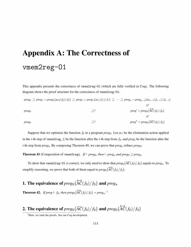
Appendix A: The Correctness of
vmem2reg-O1
This appendix presents the correctness of vmem2reg-O1 (which are fully verified in Coq). The following
diagram shows the proof structure for the correctness of vmem2reg-O1.
prog0 ⊇ prog1 = prog0{ac0( f0)/ f0} ⊇ prog2 = prog1{ac1( f1)/ f1} ⊇ ·· · ⊇ progn = progn−1{acn−1( fn−1)/ fn−1}
= ?
prog0 ⊇? prog′ = prog0{←→AC( f0)/ f0}
= ?
prog0 ⊇? prog′′ = prog0{AC( f0)/ f0}
Suppose that we optimize the function f0 in a program prog0. Let aci be the elimination action applied
in the i-th step of vmem2reg, fi be the function after the i-th step from f0, and progi be the function after the
i-th step from prog0. By composing Theorem 40, we can prove that progn refines prog0:
Theorem 41 (Composition of vmem2reg). If ` prog0, then ` progn and prog0 ⊇ progn.
To show that vmem2reg-O1 is correct, we only need to show that prog0{AC( f0)/ f0} equals to progn. To
simplify reasoning, we prove that both of them equal to prog0{←→AC( f0)/ f0}.
1. The equivalence of prog0{←→AC( f0)/ f0} and progn
Theorem 42. If prog ` f0, then prog0{←→AC( f0)/ f0}= progn. 1
2. The equivalence of prog0{AC( f0)/ f0} and prog0{←→AC( f0)/ f0}
1Here, we omit the proofs. See our Coq development.
113
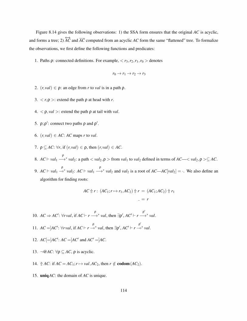
Figure 8.14 gives the following observations: 1) the SSA form ensures that the original AC is acyclic,
and forms a tree; 2)←→AC and AC computed from an acyclic AC form the same “flattened” tree. To formalize
the observations, we first define the following functions and predicates:
1. Paths ρ: connected definitions. For example, < r3,r2,r1,r0 > denotes
r0→ r1→ r2→ r3
2. (r,val) ∈ ρ: an edge from r to val is in a path ρ.
3. < r,ρ >: extend the path ρ at head with r.
4. < ρ,val >: extend the path ρ at tail with val.
5. ρ;ρ′: connect two paths ρ and ρ′.
6. (r,val) ∈ AC: AC maps r to val.
7. ρ⊆ AC: ∀r, if (r,val) ∈ ρ, then (r,val) ∈ AC.
8. AC ` val1ρ
−→∗ val2: a path < val2,ρ > from val1 to val2 defined in terms of AC—< val2,ρ >⊆ AC.
9. AC ` val1ρ
(∗ val2: AC ` val1ρ
−→∗ val2 and val2 is a root of AC—AC[val2] = ·. We also define an
algorithm for finding roots:
AC ⇑ r : (AC1;r 7→ r1,AC2) ⇑ r = (AC1;AC2) ⇑ r1
= r
10. AC⇒ AC′: ∀r val, if AC ` rρ
−→∗ val, then ∃ρ′, AC′ ` rρ′
−→∗ val.
11. AC =]AC′: ∀r val, if AC ` rρ
(∗ val, then ∃ρ′, AC′ ` rρ′
(∗ val.
12. AC[=]AC′: AC =]AC′ and AC′ =]AC.
13. ¬@AC: ∀ρ⊆ AC, ρ is acyclic.
14. ⇑ AC: if AC = AC1;r 7→ val,AC2, then r /∈ codom(AC2).
15. uniqAC: the domain of AC is unique.
114
16. 2AC: ∀(r1,r2) ∈ AC,¬∃val.(r2,val) ∈ AC.
2.1 AC is well-formed
Lemma 43. If prog ` f , f header{b}= f , and AC = flat map (rev (snd (find stld pairs block r (STLD INIT,
/0)))) b, then uniqAC and ¬@AC.
2.2 The equivalence of AC and−→AC
We first prove the facts about substituting codomains of AC—AC{val/r}, which are useful for reasoning
about−→AC.
Lemma 44. If (r,val) ∈ AC and ¬val usesr′, then (r,val) ∈ AC{val′/r′}.
Lemma 45. If AC ` rρ
−→∗ val and r′ /∈ rl < val,ρ >, then AC{val′/r′} ` rρ
−→∗ val (Here, rl denotes
removelast.)
Proof (sketch): Because r′ /∈ rl < val,ρ >, all targets of the edges in < val,ρ > do not use r′. By
Lemma 44, we prove that AC{val′/r′} has the same path from r to val.
Lemma 46. If (r′,val′) /∈ AC and (r′,val′) ∈ AC{val/r}, then (r′,r) ∈ AC and val = val′.
Lemma 47. If (r′,r) ∈ AC, then (r′,val) ∈ AC{val/r}.
Lemma 48. If uniqAC, ¬@AC and (r,val) ∈ AC, then AC =]AC{val/r}.
Proof (sketch): Consider AC ` r0
ρ
(∗ val0. If r /∈ rl < val0,ρ >, Lemma 45 concludes. If r ∈ rl <
val0,ρ >, by uniqAC, ¬@AC and that val0 is a root, we can partition < val0,ρ > as below:
r0
ρ1
−→∗ r′→ r→ valρ2
(∗ val0
Here, r /∈ rl < r′,ρ1 > and r /∈< val0,ρ2 >.
Consider the path ρ′:
r0
ρ1
−→∗ r′→ valρ2
(∗ val0
By Lemma 47, (r′,val) ∈ AC{val/r}. By Lemma 45, AC{val/r} ` r0
ρ1
−→∗ r′ and AC{val/r} ` valρ2
−→∗
val0. This concludes the proofs.
115
Lemma 49. If uniqAC and (r,val) ∈ AC, then AC{val/r}⇒ AC.
Proof (sketch): Consider AC{val/r} ` r0
ρ′
−→∗ val0. We can partition ρ′ as below:
r0
ρ0
−→∗ r′0→ val′0ρ1
−→∗ r′1→ val′1 · · ·r′n→ val′nρn
−→∗ val0
Here, (r′i,val′i) /∈ AC, and < r′i,ρi >⊆ AC when i < n, and < val0,ρn >⊆ AC.
We construct the path ρ:
r0
ρ0
−→∗ r′0→ r→ valρ1
−→∗ r′1→ r→ val · · ·r′n→ r→ valρn
−→∗ val0
Lemma 46 shows that (r′i,r) ∈ AC and val′i = val. Therefore, AC ` r0
ρ
−→∗ val0.
By Lemma 48 and Lemma 49, we have that:
Lemma 50. If uniqAC, ¬@AC and (r,val) ∈ AC, then AC{val/r}[=]AC.
By Lemma 49, we have that:
Lemma 51. If uniqAC, (r,val) ∈ AC, and ¬@AC, then ¬@AC{val/r}.
Lemma 52. If ¬val usesr, then r /∈ codom(AC{val/r}).
Lemma 53. If uniqAC, then uniq(AC{val/r}).
We also need the following properties about weakening:
Lemma 54. If AC1⇒ AC2, then AC;AC1⇒ AC;AC2.
Proof. By induction of AC. Consider the inductive case AC = r0 7→ val0,AC′. Consider AC;AC1 ` rρ
−→∗
val. Partition < r,ρ > into
rρ0
−→∗ r0→ val0ρ1
−→∗ r0→ val0 · · ·r0→ val0ρn
−→∗ val
where (r0,val0) /∈< r,ρ0 > and (r0,val0) /∈< val0,ρi > where i > 0.
Consider each AC;AC1 ` valiρi
−→∗ val′i . Because (r0,val0) /∈< vali,ρi > and IH, AC′;AC2 ` valiρ′i−→∗
val′i . So, AC;AC2 ` valiρ′i−→∗ val′i . The proof concludes by ρ′ :
rρ′0−→∗ r0→ val0
ρ′1−→∗ r0→ val0 · · ·r0→ val0
ρ′n−→∗ val
116
Lemma 55. If AC1 =]AC2, uniq(AC;AC1) and domAC1 = domAC2, then AC;AC1 =]AC;AC2.
Proof. By induction of AC. Consider the inductive case AC = r0 7→ val0,AC′. Consider AC;AC1 ` rρ
(∗ val.
Partition < r,ρ > into
rρ0
−→∗ r0→ val0ρ1
−→∗ r0→ val0 · · ·r0→ val0ρn
(∗ val
where (r0,val0) /∈< r,ρ0 > and (r0,val0) /∈< val0,ρi > where i > 0.
Consider each AC;AC1 ` valiρi
−→∗ val′i . Because (r0,val0) /∈< vali,ρi >, AC′;AC1 ` valiρi
−→∗ val′i . By
uniq(AC;AC1), AC′;AC1 ` valiρi
(∗ val′i . By IH, AC′;AC2 ` valiρ′i(∗ val′i . So, AC;AC2 ` vali
ρ′i−→∗ val′i .
Because val0 is the root of AC;AC1 and domAC1 = domAC2, val0 must also be the root of AC;AC2.
The proof concludes by ρ′:
rρ′0−→∗ r0→ val0
ρ′1−→∗ r0→ val0 · · ·r0→ val0
ρ′n(∗ val
By Lemma 55, we have:
Lemma 56. If AC1[=]AC2, uniq(AC;AC1), uniq(AC;AC2) and domAC1 = domAC2, then AC;AC1[=
]AC;AC2.
By Lemma 54, we have:
Lemma 57. If AC2⇒ AC1, then ¬@AC;AC1 ⇒ ¬@AC;AC2.
With the above properties, we prove that AC and−→AC are equivalent.
Lemma 58. If uniqAC and ¬@AC, then−→AC[=]AC.
Proof. By induction on the length of AC. The base case is trivial. Consider the case AC = r 7→ val,AC′. We
have−→AC = r 7→ val,
−−−−−−−−−→(AC′{val/r}). By Lemma 50, AC[=]r 7→ val{val/r},AC′{val/r}. Because of ¬@AC,
val{val/r}= val. We conclude by IH and Lemma 56.
2.3 The equivalence of AC and←−AC
Lemma 59.
117
1. If ¬@AC, r ∈ dom(AC)∨ r ∈ codom(AC) and AC ⇑ r = val, then AC ` rρ
(∗ val.
2. If uniqAC, ¬@AC and AC ` rρ
(∗ val, then AC ⇑ r = val.
Lemma 60.
1. AC[r] = bcnstc iff−→AC[r] = bcnstc.
2. AC[r] = · iff −→AC[r] = ·.
Lemma 61. If uniqAC and ¬@AC, then−→AC⇒ AC and ¬@
−→AC.
By Lemma 58, Lemma 60, Lemma 59 and Lemma 61,
Theorem 62. If uniqAC and ¬@AC, then AC ⇑ r =−→AC ⇑ r.
Lemma 63. If r /∈ dom(AC) and r /∈ codom(AC), then r /∈ codom(−→AC).
All elements in−→AC are sorted in terms of AC—⇑ −→AC.
Lemma 64. If uniqAC and ¬@AC, then ⇑ −→AC.
Proof (sketch): By induction on the length of AC. Consider the case AC = r 7→ val,AC′ and−→AC = r 7→
val,−−−−−−−−−→(AC′{val/r}). By Lemma 51 and Lemma 53, ¬@AC′{val/r} and uniqAC′{val/r}.
Let−→AC = AC1;r1 7→ val1,AC2. If (r1,val1) ∈ AC′{val/r}, the proof is by IH—⇑ AC′{val/r}. Other-
wise, if r1 = r and val1 = val, the proof is by Lemma 52 and Lemma 63.
Lemma 65. If uniq(AC1;r1 7→ r2,AC2), then (AC1;r1 7→ r2,AC2)(r1) = AC2(r2).
Lemma 66. If uniq(AC1;r1 7→ r2,AC2) and ⇑ (AC1;r1 7→ r2,AC2), then (AC1;AC2) ⇑ r2 = AC2 ⇑ r2.
Lemma 67. If uniqAC and ⇑ AC, then AC(r) = AC ⇑ r.
Proof (sketch): By induction on the length of AC. It is trivial if AC does not map r. Consider the case
AC = AC1;r 7→ r′,AC2.
AC ⇑ r = (AC1;AC2) ⇑ r′ definition
= AC2 ⇑ r′ By Lemma 66
= AC2(r′) By IH
= AC(r′) By Lemma 65
118
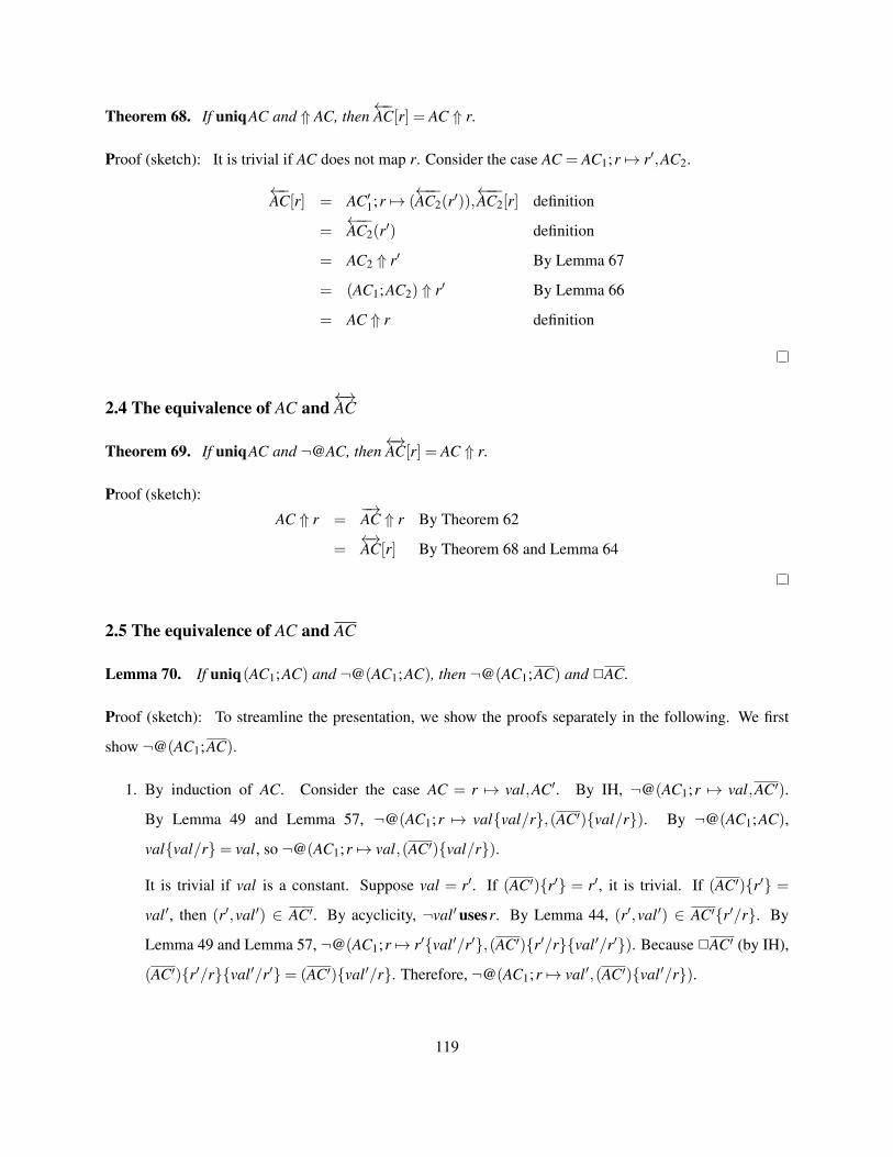
Theorem 68. If uniqAC and ⇑ AC, then←−AC[r] = AC ⇑ r.
Proof (sketch): It is trivial if AC does not map r. Consider the case AC = AC1;r 7→ r′,AC2.
←−AC[r] = AC′1;r 7→ (
←−−AC2(r′)),
←−−AC2[r] definition
=←−−AC2(r′) definition
= AC2 ⇑ r′ By Lemma 67
= (AC1;AC2) ⇑ r′ By Lemma 66
= AC ⇑ r definition
2.4 The equivalence of AC and←→AC
Theorem 69. If uniqAC and ¬@AC, then←→AC[r] = AC ⇑ r.
Proof (sketch):
AC ⇑ r =−→AC ⇑ r By Theorem 62
=←→AC[r] By Theorem 68 and Lemma 64
2.5 The equivalence of AC and AC
Lemma 70. If uniq(AC1;AC) and ¬@(AC1;AC), then ¬@(AC1;AC) and 2AC.
Proof (sketch): To streamline the presentation, we show the proofs separately in the following. We first
show ¬@(AC1;AC).
1. By induction of AC. Consider the case AC = r 7→ val,AC′. By IH, ¬@(AC1;r 7→ val,AC′).
By Lemma 49 and Lemma 57, ¬@(AC1;r 7→ val{val/r},(AC′){val/r}). By ¬@(AC1;AC),
val{val/r}= val, so ¬@(AC1;r 7→ val,(AC′){val/r}).
It is trivial if val is a constant. Suppose val = r′. If (AC′){r′} = r′, it is trivial. If (AC′){r′} =
val′, then (r′,val′) ∈ AC′. By acyclicity, ¬val′usesr. By Lemma 44, (r′,val′) ∈ AC′{r′/r}. By
Lemma 49 and Lemma 57, ¬@(AC1;r 7→ r′{val′/r′},(AC′){r′/r}{val′/r′}). Because 2AC′ (by IH),
(AC′){r′/r}{val′/r′}= (AC′){val′/r}. Therefore, ¬@(AC1;r 7→ val′,(AC′){val′/r}).
119
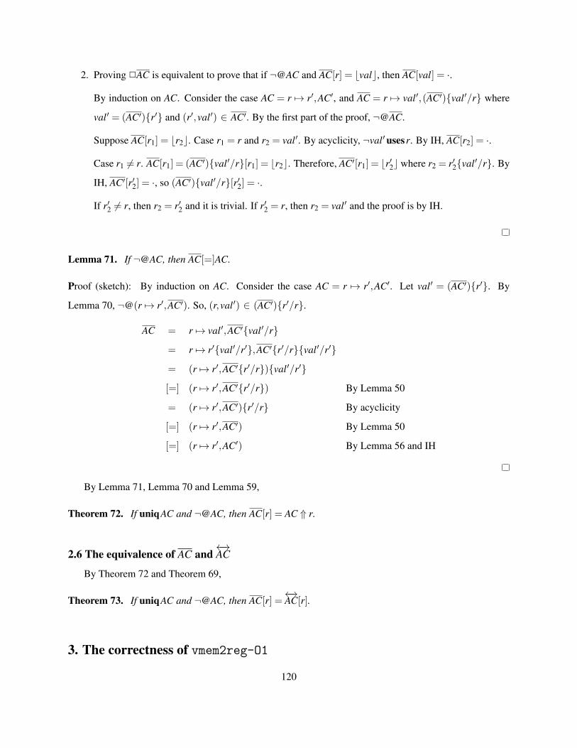
2. Proving 2AC is equivalent to prove that if ¬@AC and AC[r] = bvalc, then AC[val] = ·.
By induction on AC. Consider the case AC = r 7→ r′,AC′, and AC = r 7→ val′,(AC′){val′/r} where
val′ = (AC′){r′} and (r′,val′) ∈ AC′. By the first part of the proof, ¬@AC.
Suppose AC[r1] = br2c. Case r1 = r and r2 = val′. By acyclicity, ¬val′usesr. By IH, AC[r2] = ·.
Case r1 6= r. AC[r1] = (AC′){val′/r}[r1] = br2c. Therefore, AC′[r1] = br′2c where r2 = r′2{val′/r}. By
IH, AC′[r′2] = ·, so (AC′){val′/r}[r′2] = ·.
If r′2 6= r, then r2 = r′2 and it is trivial. If r′2 = r, then r2 = val′ and the proof is by IH.
Lemma 71. If ¬@AC, then AC[=]AC.
Proof (sketch): By induction on AC. Consider the case AC = r 7→ r′,AC′. Let val′ = (AC′){r′}. By
Lemma 70, ¬@(r 7→ r′,AC′). So, (r,val′) ∈ (AC′){r′/r}.
AC = r 7→ val′,AC′{val′/r}
= r 7→ r′{val′/r′},AC′{r′/r}{val′/r′}
= (r 7→ r′,AC′{r′/r}){val′/r′}
[=] (r 7→ r′,AC′{r′/r}) By Lemma 50
= (r 7→ r′,AC′){r′/r} By acyclicity
[=] (r 7→ r′,AC′) By Lemma 50
[=] (r 7→ r′,AC′) By Lemma 56 and IH
By Lemma 71, Lemma 70 and Lemma 59,
Theorem 72. If uniqAC and ¬@AC, then AC[r] = AC ⇑ r.
2.6 The equivalence of AC and←→AC
By Theorem 72 and Theorem 69,
Theorem 73. If uniqAC and ¬@AC, then AC[r] =←→AC[r].
3. The correctness of vmem2reg-O1
120
By Theorem 41, Theorem 73, Lemma 43 and Theorem 42,
Theorem 74 (vmem2reg-O1 is correct). If f ′ = vmem2reg-O1 f and ` prog, then ` prog{ f ′/ f} and
prog⊇ prog{ f ′/ f}.
121
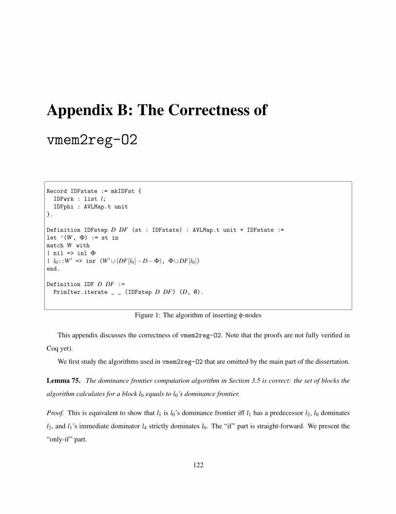
Appendix B: The Correctness of
vmem2reg-O2
Record IDFstate := mkIDFst {
IDFwrk : list l;IDFphi : AVLMap.t unit
}.
Definition IDFstep D DF (st : IDFstate) : AVLMap.t unit + IDFstate :=
let ’(W, Φ) := st in
match W with
| nil => inl Φ
| l0::W ′ => inr (W ′∪ (DF [l0]−D−Φ), Φ∪DF [l0])end.
Definition IDF D DF :=
PrimIter.iterate _ _ (IDFstep D DF) (D, /0).
Figure 1: The algorithm of inserting φ-nodes
This appendix discusses the correctness of vmem2reg-O2. Note that the proofs are not fully verified in
Coq yet).
We first study the algorithms used in vmem2reg-O2 that are omitted by the main part of the dissertation.
Lemma 75. The dominance frontier computation algorithm in Section 3.5 is correct: the set of blocks the
algorithm calculates for a block l0 equals to l0’s dominance frontier.
Proof. This is equivalent to show that l1 is l0’s dominance frontier iff l1 has a predecessor l2, l0 dominates
l2, and l1’s immediate dominator l4 strictly dominates l0. The “if” part is straight-forward. We present the
“only-if” part.
122
Suppose l2 is l1’s predecessor, l0 dominates l2 and does not strictly dominates l1. Because dominance
relations form a tree, the tree path to l1 and the tree path to l2 must have the same prefix.
Suppose the path of l2 joins l1’s at l3 that strictly dominates l1’s immediate dominator l4. Then, there
must exist a path ρ to l2 that does not go through l4. Otherwise, l4 must strictly dominate l2, and the tree
paths of l1 and l2 must join at l4. However, ρ also reaches l1. This is contradictory to that l4 strictly dominates
l1. Therefore, l4 must be in the same prefix of the two tree paths.
l0 cannot dominate l4. Otherwise l0 strictly dominate both l1 and l2. Therefore, l0 must be in the set of
blocks calculated by the algorithm.
Figure 1 shows the algorithm that calculates where to insert φ-node [8]: given a promotable location,
all the dominance frontiers of the definitions at the location need φ-nodes. The definitions of a promotable
location include alloca’s of the location, store’s to the location and inserted φ-nodes for the location. There-
fore, the algorithm needs to iteratively insert φ-nodes until all the inserted φ-nodes also satisfy the above
requirement.
The algorithm is implemented by a primitive recursion (PrimIter.iterate) based on a worklist.
IDFstate defines calculation states of each recursion step: IDFwrk is the worklist that records blocks
to process; IDFphi is the blocks that need to insert φ-nodes. Initially, the worklist includes blocks all
with original definitions (which are denoted by D, and only contain alloca’s and store’s) of a promotable
locations. IDFstep, given D and dominance frontiers DF , implements each recursion step. If the current
worklist is empty, IDFstep returns the inserted φ-nodes, and stops the entire recursion. Otherwise, IDFstep
picks a block from the worklist, adds the dominance frontiers that do not have the original and inserted
definitions to the worklist, and inserts φ-nodes for the dominance frontiers.
Lemma 76. IDF (in Figure 1) terminates.
Proof. Consider the following measure function:
M(W,Φ) = |W |+N ∗ (N−|Φ|)
Here, || computes the size of a set; N is the number of blocks in the function IDF computes. It is sufficient
to show that
1. M(W,Φ)≥ 0.
2. If IDF D DF (W,Φ) = inr(W ′,Φ′), then M(W,Φ)> M(W ′,Φ′).
123
The first fact is true because the number of inserted φ-nodes cannot be greater than the number of all blocks.
Suppose W = l0 :: W ′′, W ′ =W ′′∪ (DF [l0]−D−Φ) and Φ′ = Φ∪DF [l0].
M(W ′,Φ′)−M(W,Φ) = N ∗ (|Φ|− |Φ′|)+ |W ′|− |W |
= N ∗ (|Φ|− |Φ∪DF [l0]|)+ |W ′′∪ (DF [l0]−D−Φ|−1−|W ′′|
Consider two cases. The first case is when DF [l0] 6⊂Φ.
M(W ′,Φ′)−M(W,Φ) ≤ N ∗ (|Φ|− (|Φ|+1))+ |W ′′∪Φ|−1−|W ′′|
≤ N ∗ (|Φ|− (|Φ|+1))+ |W ′′|+ |Φ|−1−|W ′′|
= −N + |Φ|−1
< 0
The second case is when DF [l0]⊂Φ.
M(W ′,Φ′)−M(W,Φ) = N ∗ (|Φ|− |Φ|)+ |W ′′|−1−|W ′′|
< 0
Lemma 77. IDF is correct: if IDF D DF (D, /0) = inlΦ, then ∀l0 ∈ D∪Φ, DF [l0]⊂ D∪Φ.
Proof. In general, consider the following invariant:
INV DDF (W,Φ) = ∀l0 ∈ D∪Φ, l0 ∈W ∨DF [l0]⊂ D∪Φ
It is sufficient to show that
If IDF D DF (W,Φ) = inr(W ′,Φ′) and INV DDF (W,Φ), then INV DDF (W ′,Φ′).
It is trivial if W is empty. Consider W = l1 :: W ′′, W ′ = W ′′ ∪ (DF [l1]−D−Φ) and Φ′ = Φ∪DF [l1].
Suppose l0 ∈ D∪Φ′.
1. l0 ∈ D∪Φ: By assumption, l0 ∈W ∨DF [l0]⊆ D∪Φ.
a) l0 ∈W = l1 :: W ′′:
i. l0 = l1: DF [l1]⊆Φ∪DF [l1] = Φ′ ⊆ D∪Φ′
ii. l0 ∈W ′′: l0 ∈W ′ =W ′′∪ (DF [l1]−D−Φ)
b) DF [l0]⊆ D∪Φ: DF [l0]⊆ D∪ (Φ∪DF [l1]) = D∪Φ′:
124

2. l0 ∈ DF [l1]∧ l0 /∈ D∪Φ: l0 ∈ (DF [l1]−D−Φ)⊆W ′ =W ′′∪ (DF [l1]−D−Φ).
By Lemma 75 and the proofs in [28], we have that
Lemma 78. Given the dominance frontier calculated by the algorithm in Section 3.5, IDF and the iterated
path-convergence criterion [8] specify exactly the same set of nodes at which to put φ-nodes.
By Lemma 75 and Lemma 77, we prove that
Lemma 79. After the φ-node insertion of vmem2reg-O2, given a load to r1 from a promotable location,
1. If there exists a store with value val2 to the promotable location at program counter pc2 and the store
is the closest one that dominates the load, we have LAS (r1, pc2, val2): in other words, there are no
other store’s to the location between the load and the store.
2. Otherwise, we have LAA r1: in other words, there are no other store’s to the location between the
load and the alloca.
Proof. We present the proofs of the first fact. Suppose between pc2 and r1 there exists a simple path ρ that
goes through another store to the location. Consider the closest store at pc3 to r1 on ρ. Because pc2 is the
closest store that dominates r1, there must exist a path ρ′ from pc2 to r1 that bypasses pc3, and ρ and ρ′
join between pc3 and r1. In terms of the iterated path-convergence criterion and Lemma 78, a φ-node and a
corresponding store must be inserted at the joint point. Therefore, pc3 is not the closest store to r1 on ρ.
Finally, by Lemma 79, we need the following extended lemma for reasoning about vmem2reg-O2.
Lemma 80. LAS/LAA are correct with respect to arbitrary domination relations (Section 8.3 requires that
domination relations must be in the same block).
125