FORMAL VERIFICATION OF THERMAL AWARE

ARCHITECHTURES FOR MULTI CORE SYSTEMS

By

MUHAMMAD ISMAIL

2010-NUST-MS-EE(S)-23

Supervisor:

Dr. Osman Hasan

A thesis submitted in partial fulfillment of the requirements for the degree of

Masters of Science in Electrical Engineering

School of Electical Engineering and Computer Science,

National University of Sciences and Technology (NUST), Islamabad,

Pakistan.

(March 2013)

c©Copyright

by

Muhammad Ismail

2012

ii

to my

FAMILY

iii

Acknowledgements

I would like to express my very great appreciation to Dr. Osman Hasan, my research

supervisor, who gave me opportunity to work on formal verification. Thanks for his

professional guidance, enduring patience, encouragement, valuable and constructive

suggestions during this research work. His willingness to give his time so promptly

and generously has been very much appreciated. I want to extend my thanks to

one of our RCMS seniors Usman Rauf, for his help on providing solution to a few

modeling problems.

I thank and appreciate Dr. Zahid Anwar for his guidance for including time

analysis in the model. Special Thanks to Mr. Thomas Ebi and Mohamed Shafique,

members of KIT, for taking out time for meetings and providing constructive and

useful recommendations on this project.

Finally, I wish to thank my parents for their continuous help, support and

encouragement throughout my study. Without their financial and spiritual support,

I wasn’t able to complete it.

NOTE: This thesis was submitted to my Supervising Committee on the March 15,

2013.

iv

Abstract

With the recent developments in nano-fabrication technology, transistor density per

unit area is increasing considerably. This in turn leads to an increase in the heat

generated per unit area due to more switching of transistors. Various distributed

thermal management techniques have been proposed to tackle this overheating

problem. Analyzing the reliability and efficiency of these thermal management

techniques is a major challenge given their distributed nature and the involvement

of a large number of parameters.

Simulation is the state-of-the-art analysis technique used for distributed thermal

management schemes. Due to inherent approximate nature of simulation, it cannot

ascertain 100% reliable analysis. Moreover, no one can guarantee that all the

potential corner cases have been checked due to the numerous parameters involved

and the distributed nature of the underlying scheme.

To overcome these limitations, we propose a methodology to perform their formal

verification in this thesis. Formal verification is a computer based mathematical

analysis technique and given its mathematical nature, it can guarantee accurate

results. The proposed methodology is primarily based on the SPIN model checker

and the Lamport timestamps algorithm and it allows verification of both functional

and timing properties. For illustration, this thesis presents the analysis of Thermal-

aware Agent-based Power Economy (TAPE), which is a recently proposed agent

based dynamic thermal management approach.

v

Table of Contents

Page

Acknowledgements . . . . . . . . . . . . . . . . . . . . . . . . . . . . . . . . iv

Abstract . . . . . . . . . . . . . . . . . . . . . . . . . . . . . . . . . . . . . . v

Table of Contents . . . . . . . . . . . . . . . . . . . . . . . . . . . . . . . . . vi

List of Figures . . . . . . . . . . . . . . . . . . . . . . . . . . . . . . . . . . viii

List of Tables . . . . . . . . . . . . . . . . . . . . . . . . . . . . . . . . . . . ix

Chapter

1 Introduction . . . . . . . . . . . . . . . . . . . . . . . . . . . . . . . . . . 1

1.1 Thermal-Aware architectures . . . . . . . . . . . . . . . . . . . . . . 1

1.2 Problem Statement . . . . . . . . . . . . . . . . . . . . . . . . . . . 2

1.3 Proposed solution: Model checking . . . . . . . . . . . . . . . . . . 3

1.4 Outline of the Thesis . . . . . . . . . . . . . . . . . . . . . . . . . . 5

2 Preliminaries . . . . . . . . . . . . . . . . . . . . . . . . . . . . . . . . . 6

2.1 Formal verification . . . . . . . . . . . . . . . . . . . . . . . . . . . 6

2.1.1 Analysis Methods: Comparison . . . . . . . . . . . . . . . . 7

2.1.2 Model Checking . . . . . . . . . . . . . . . . . . . . . . . . . 7

2.1.3 SPIN Model Checker . . . . . . . . . . . . . . . . . . . . . . 8

3 Proposed Methodology . . . . . . . . . . . . . . . . . . . . . . . . . . . . 10

3.1 Building Promela Model . . . . . . . . . . . . . . . . . . . . . . . . 11

3.1.1 Choosing datatypes . . . . . . . . . . . . . . . . . . . . . . . 11

3.1.2 Channel Assignment . . . . . . . . . . . . . . . . . . . . . . 12

3.2 Lamport’s Timestamps . . . . . . . . . . . . . . . . . . . . . . . . . 12

3.3 Simulation . . . . . . . . . . . . . . . . . . . . . . . . . . . . . . . . 14

3.4 Checking for deadlocks . . . . . . . . . . . . . . . . . . . . . . . . . 14

vi

3.5 LTL Properties . . . . . . . . . . . . . . . . . . . . . . . . . . . . . 15

3.6 Timing Analysis . . . . . . . . . . . . . . . . . . . . . . . . . . . . . 15

4 Modeling TAPE in PROMELA . . . . . . . . . . . . . . . . . . . . . . . 17

4.1 TAPE . . . . . . . . . . . . . . . . . . . . . . . . . . . . . . . . . . 17

4.1.1 Structured macros . . . . . . . . . . . . . . . . . . . . . . . 18

4.1.2 init: An initialization process . . . . . . . . . . . . . . . . . 19

4.2 Processes and channels . . . . . . . . . . . . . . . . . . . . . . . . . 21

4.3 Temperature consideration . . . . . . . . . . . . . . . . . . . . . . . 22

4.4 Lamport Timestamps . . . . . . . . . . . . . . . . . . . . . . . . . . 23

5 Verification Results . . . . . . . . . . . . . . . . . . . . . . . . . . . . . . 25

6 Conclusions . . . . . . . . . . . . . . . . . . . . . . . . . . . . . . . . . . 30

6.1 Summary . . . . . . . . . . . . . . . . . . . . . . . . . . . . . . . . 30

6.2 Future Work . . . . . . . . . . . . . . . . . . . . . . . . . . . . . . . 30

Referencesrefs . . . . . . . . . . . . . . . . . . . . . . . . . . . . . . . . . . . 32

Appendix

A TAPE Algorithm . . . . . . . . . . . . . . . . . . . . . . . . . . . . . . . 34

vii

List of Figures

3.1 Proposed Methodology. . . . . . . . . . . . . . . . . . . . . . . . . . 10

3.2 Channel Assignment . . . . . . . . . . . . . . . . . . . . . . . . . . 12

4.1 Model Checking TAPE . . . . . . . . . . . . . . . . . . . . . . . . . . . 18

viii

List of Tables

2.1 Analysis methods . . . . . . . . . . . . . . . . . . . . . . . . . . . . . 7

5.1 Statistics of all the 12 properties verified where p0001 is related to node (0,0)

and (0,1) and so on . . . . . . . . . . . . . . . . . . . . . . . . . . . . 26

5.2 Effect of as(Total Power units:128, Tasks:10, ab:2/10, wus:2/7, wfs:2/7, wub:8/7,

wfb:2/7) . . . . . . . . . . . . . . . . . . . . . . . . . . . . . . . . . . 27

5.3 Effect of ab(Total Power units:128, Tasks:10, as:2/10, wus:2/7, wfs:2/7, wub:8/7,

wfb:2/7) . . . . . . . . . . . . . . . . . . . . . . . . . . . . . . . . . . 27

5.4 Effect of Tasks (Total Power units:128, as:2/10, ab:2/10, wus:2/7, wfs:2/7,

wub:8/7, wfb:1/7) . . . . . . . . . . . . . . . . . . . . . . . . . . . . . 29

ix

Chapter 1

Introduction

As the semiconductor industry moves towards smaller technology nodes, elevated

temperatures resulting from the increased power densities are becoming a growing

concern. As power density increases, the cooling costs also rises exponentially and

any multicore architectures can not be designed for worst case [18].

1.1 Thermal-Aware architectures

To regulate the operating temperature, there must be some runtime processor level

techniques or thermal models that must be in practical and efficient.

Localized heating is much rapid as compared to chip-wide heating and therefore

spatial power distribution is not uniform, this leads to hot spots and spatial

gradients that can cause timing errors or even physical damage. This means

that for thermal management techniques, one must directly target the spatial and

temporal behavior of operating temperature. Many low-power techniques have little

or no effect on operating temperature, because they do not reduce power density

in hot spots. Temperature-aware design is therefore a distinct solution [18].

Power-aware design alone has failed, requiring temperature-aware design at

all system levels, including the processor architecture [18]. Dynamic Thermal

Management (DTM) of distributed nature has been identified as one of the key

reliability challenges in the ITRS roadmap [11]. DTM includes temperature,

Dynamic Voltage and Frequency Scaling(DVFS) and migrating tasks to spare units.

At the same time, the growing integration density is paving the way for future

many-core systems consisting of hundreds and even thousands of cores on a single

chip [4].

From a thermal management perspective, these systems bring both new oppor-

tunities as well as new challenges. DTM in single-core systems is largely limited to

Dynamic Voltage and Frequency Scaling (DVFS), many-core systems present the

possibility for spreading power consumption in order to balance temperature over

a larger area through the mechanism of task migration. However, the increased

problem space related to the large number of cores makes the complexity of DTM

grow considerably.

Traditionally, DTM decisions have been made using centralized approaches

with global knowledge. These, however, quickly become infeasible due to lack

of scalability when entering the many-core domain [7]. As a result, distributed

thermal management schemes have emerged [5,7,8] which tackle the complexity

and scalability issues of many-core DTM by transforming the problem space from

a global one to many smaller regional ones which can exploit locality when making

DTM decisions. For a distributed DTM scheme to achieve the same quality as

is possible from one using global knowledge, however, it becomes necessary for

there to be an exchange of state information across regions in order to negotiate

a near-optimal system state configuration [7]. The choice of tuning parameters

for this negotiation has been identified as a critical issue in ensuring a stable

system [12].

1.2 Problem Statement

Up until now these distributed DTM schemes have been exclusively analyzed using

either simulations or running on real systems. However, due to the non-exhaustive

2

nature of simulation, such analysis alone is not enough to account for and guarantee

stability in all possible system configurations. Even if some corner cases can be

specifically targeted, there is no proof that these represent a worst-case scenario,

and it is never possible to consider or even foresee all corner cases. Moreover, using

simulation we may show that for a given set of tasks and cores, a small number of

mappings result in localized minima. However, in distributed DTM approaches this

actually means that a local region of cores may be successfully applying DTM from

their point of view although from the global view temperatures are really maximal.

Thus, simulation based analysis cannot be considered complete and it often results

in missing critical bugs, which in turn may lead to delays in deployment of DTM

schemes as happened in the case of Foxton DTM scheme that was designed for the

Montecito chip [6].

1.3 Proposed solution: Model checking

The above mentioned limitations can be overcome by using model checking [3] for

the analysis of distributed DTM. The main principle behind model checking is to

construct a computer based mathematical model of the given system in the form of

an automata or state-space and automatically verify, within a computer, that this

model meets rigorous specifications of intended behavior. Due to its mathematical

nature, 100% completeness and soundness of the analysis can be guaranteed [2].

Moreover, the ability to provide counter examples in case of failures and the

automatic nature of model checking makes it a more preferable choice for industrial

usage as compared to the other mainstream formal verification approaches like

theorem proving.

Model checking has been successfully used for analyzing some unicore DTM

schemes (e.g., [16, 17]). Similarly, probabilistic model checking of a DTM for

3

multicore architectures is presented in [15]. The main focus of this work is to

conduct a probabilistic analysis of frequency effects through DVFS, time and power

spent over budget along with an estimate of required verification efforts. In order

to raise the level of formally verifying complex DTM schemes, statistical model

checking of power gating schemes has been recently reported [13]. However, to

the best of our knowledge, so far no formal verification method, including model

checking, has been used for the verification of a distributed DTM for many-core

systems. This paper intends to fill this gap and proposes a methodology for the

functional and timing verification of distributed DTM schemes.

The main idea behind the proposed methodology is to use the SPIN model

checker [10], which is an open source tool for the formal verification of distributed

software systems, and Lamport timestamps [14], which is an algorithm that allows

us to determine the order of events in a distributed system execution. We can

formally model or specify the behavoir of distributed DTM schemes in the PROcess

MEta LAnguage (PROMELA) language. These models can then be verified to

exhibit the desired functional properties using the SPIN model checker as it directly

accepts PROMELA models. Lamport timestamps algorithm is introduced in the

PROMELA model of the given distributed DTM scheme to facilitate the verification

of timing properties via the SPIN model checker.

In order to illustrate the utilization and effectiveness of the proposed methodol-

ogy for the formal verification of real-world distributed DTM schemes, we present

the analysis of Thermal-aware Agent-based Power Economy (TAPE) [7], which is a

recently proposed agent based distributed DTM approach. The main reason behind

the choice of this case study is its enormous effectiveness in hot-spot avoidance

compared to traditional techniques like PDTM and HRTM.

4

1.4 Outline of the Thesis

The rest of the thesis report is organized as follows: The proposed methodology

is presented in chapter 3. This is followed by the formal modeling of the TAPE

algorithm in chapter 4. Next, we present the formal verification of functional and

timing properties of TAPE in chapter 5. Finally, chapter 5 concludes the thesis.

We have provided an overview of formal verification, model checking and the SPIN

model checker in chapter 2 to aid the understanding of this work for the readers

with limited know-how about model checking.

5

Chapter 2

Preliminaries

In this chapter, we present some foundational material about basics of formal

verification with focus on model checking and SPIN model checker to facilitate

understanding of this thesis.

2.1 Formal verification

Formal methods is the use of ideas and techniques from applied mathematics and

formal logic to specify, analyze and reason about computing systems to increase

design assurance and eliminate defects. Aim is to verify and develop a safety critical

software and hardware with less cost and effort, while still satisfying the highest

reliability requirements. Both software and hardware systems today are used in

applications where failure or even a small bug is not acceptable and can lead to

either loss of lives or financial burden.

In todays multi/many-core architectures and complex embedded systems design

development, the most critical element is functional and logical verification. This

complexity also increases verification complexity and even more challenging. In

complex and large systems, usually the time spent on verification is much more

than on construction due to exhaustive nature. For reduction of verification time,

formal methods provide effective techniques.

2.1.1 Analysis Methods: Comparison

Here comparison of few analysis methods are shown in table 2.1. Paper pencil

proof is a very tedious and time consuming option, but have accuracy. Contrary

to this simulation automatic. In fact, the simulation is inherently incomplete, no

matter how the simulation is long and how intelligent the testbench is. Therefore

as alternatives, formal verification techniques have been proposed.

Table 2.1: Analysis methods

Criteria Paper and Pencil Proof Simulation Model Checking

Accuracy 2� 4 2�Automation 4 2� 2�

Formal verification explores all possible states exhaustively. Model checking is

an automatic formal verification technique that has both accuracy and completeness.

No human interaction required after developing of the model and specifying its

desired properties.

2.1.2 Model Checking

Model checking [3] is primarily used as the verification technique for reactive, finite

state concurrent systems, i.e., the systems whose behavior is dependent on time

and their environment, like controller units of digital circuits and communication

protocols. The inputs to a model checker include the finite-state model of the

system that needs to be analyzed along with the intended system properties, which

are expressed in temporal logic. The model checker automatically and exhaustively

verifies if the properties hold for the given system while providing an error trace

in case of a failing property. The state-space of a system can be very large, or

sometimes even infinite. Thus, it becomes computationally impossible to explore

the entire state-space with limited resources of time and memory. This problem,

7

termed as state-space explosion, is usually resolved by developing abstract, less

complex, models of the system. Moreover, many efficient algorithms and techniques,

like symbolic and bounded model checking, have been proposed to alleviate the

memory and computation requirements of model checking. The above mentioned

methods along with appropriate usage of abstraction have enabled a wide usage of

model checking. Some of the commonly used model checking tools include SPIN

(used for distributed systems), NuSMV (used for concurrent systems), Uppaal (used

for real-time Systems), Hytech (used for hybrid systems) and PRISM (used for

probabilistic analysis).

2.1.3 SPIN Model Checker

SPIN model checker [10], developed by Bell Labs, is a widely used formal verification

tool for analyzing distributed and concurrent software systems. SPIN has support

for random, interactive and guided simulation, and both exhaustive and partial

proof techniques. The system that needs to be verified is expressed in a high-level

language PROMELA, which is based on Dijkstra’s guarded command language

and has a syntax that is quite similar to the C programming language. The

behavior of the given distributed system is expressed using asynchronous processes.

Every process can have multiple instantiations to model cases where multiple

distributed modules with similar behavior exist. The processes can communicate

with one another via synchronous (rendezvous) or asynchronous (buffered) message

channels. Both global and local variables of boolean, byte, short, int, unsigned

and single dimensional arrays can be declared. Defining new data types is also

supported. Once the system model is formed in PROMELA then it is automatically

translated to a automaton or state-space graph by SPIN. This step is basically

done by translating each process to its corresponding automaton first and then

forming an asynchronous interleaving product of these automata to obtain the

8

global behavior [10].

The properties to be verified can be specified in SPIN using Linear Temporal

Logic (LTL) or assertions. LTL allows us to formally specify time-dependant

properties using both logical (conjunction (&&), disjunction (‖), negation (!),

implication(->) and equality (<->) and temporal operators, i.e., always ([]), even-

tually (<>), next (X) and until (∪). For example, for two state-dependant predicates

p and q, we can formally specify that q occurs in response to p in LTL, i.e., p

implies eventually q as (p -> (<>q)). For verification, the given property is first

automatically converted to a Buchi automaton and then its synchronous product

with the automaton representing the global behavior is formed by the SPIN model

checker. Next, an exhaustive verification algorithm, like the Depth First Search

(DFS), is used to check if the property holds for the given model or not. The

verification is done automatically and the only two inputs required from the user

are the PROMELA model of the system and the LTL properties that need to be

verified. Besides verifying the logical consistency of a property, SPIN can also be

used to check for the presence of deadlocks, race conditions, unspecified receptions

and incompleteness. Moreover, SPIN also supports random, interactive and guided

simulation, which is a very helpful utility for debugging.

The SPIN model checker has been extensively used for verifying many real-world

systems including distributed software systems, data communications protocols,

switching systems etc. However, to the best of our knowledge it has never been

used for verifying any DTM scheme, which is the contribution of the present paper.

9

Chapter 3

Proposed Methodology

The most critical functional aspect of any distributed DTM scheme is its ability to

reach near-optimal system state configuration from all possible scenarios. Moreover,

the time required to reach such a stable state and the effect of various parameters on

this time is the most interesting timing related behavior. The proposed methodology,

depicted in Figure 3.1, utilizes the SPIN model checker to verify properties related

to both of these aspects for any given distributed DTM scheme.

1.PROMELA MODEL(processes, channels,

Variable Abstractions,Lamport Timestamps)

2.SIMULATION

(to see behavior)

Fail3.

CHECK FORDEADLOCKS

Pass

6a.DEBUG

(Rerun coun-terexample using

simulation)

Fail

4.LTL PROPERTYSPECIFICATION

Pass

5.FUNCTIONAL

VERIFICATION

Fail

7.TIMING VER-

IFICATION

Pass

6b.SIMPLIFICATION

AND OPTI-MIZATION

Out of memoryor

State Space explosion

Figure 3.1: Proposed Methodology.

3.1 Building Promela Model

The first step is to construct the PROMELA model of the given distributed DTM

system. For this purpose, we have to individually describe each autonomous node

of the system using one or more processes. Each process description will also

include message channels for representing their interactions with other processes.

Moreover, an initialization process should also be used to assign initial values to

the variables used to represent the physical starting conditions of the given DTM

system. The coding can be done in a quite straightforward manner due to the C

like syntax of PROMELA. However, choosing the most appropriate data type for

each variable of the given scheme can be a bit challenging.

3.1.1 Choosing datatypes

Due to the extensive interaction of DTM schemes with their continuous sur-

roundings, some of the variables used in such schemes are continuous in nature.

Temperature is a foremost example in this regard. However, due to the automata

based verification approach of model checking, variables with infinite precision

cannot be handled.

State-space explosion problem

Choosing datatypes and big size variables usage often results in state space explosion

problem because of the large number of their possible combinations. Unlike C,

Float datatype is not supported. Therefore, we have to discretize all the real

or floating-point variables of the given DTM scheme. The lesser the number of

possible values, the faster would be the verification. It is important to note that

the discretization of the variables is not a big concern here since the main focus of

model-checking is not computation of exact values but functional verification while

11

covering all the possible scenarios.

3.1.2 Channel Assignment

(0,0) (0,1)

(1,0) (1,1)

(0,2)

(1,2)

(2,0) (2,1) (2,2)

5

0

1

2

35 31 27

16

20

24

143 2219

2623

107

30113415

13

17

4

6 18

9

12

21

8

29

32

33

25

28

Figure 3.2: Channel Assignment

The channel assignment shown in fig 3.2for sharing data between nodes is done

in a highly generalized fashion. This makes the extension of the model much easy

without changing the previously assigned channels to a smaller number of nodes.

Only thing needed is to assign further channels to the newly added nodes and the

process instantiation for it.

3.2 Lamport’s Timestamps

Just like any verification exercise of engineering systems, the verification of timing

properties of distributed DTM schemes is a very important aspect. For example,

12

we are interested in the time required to reach a stable state after the n tasks are

equally mapped to different tiles in a distributed DTM scheme. However, due to

the distributed nature of these schemes, formal specification and verification of

timing properties is not a straightforward task as we may be unable to distinguish

between which one of the two occurring events occurred first. Lamport timestamps

algorithm [14] provides a very efficient solution to this problem. The main idea

behind this algorithm is to associate a counter with every node of the distributed

system such that it increments once for every event that takes place in that node.

The total ordering of all the events of the distributed system is achieved by ensuring

that every node shares its counter value with any other node that it communicates

with and it updates its counter value whenever it receives a value greater than its

own counter value.

In this work, we propose to utilize Lamport timestamps algorithm to determine

the total number of events in the PROMELA model of the given distributed DTM

scheme. The main advantage of this choice is that we can utilize the SPIN model

checker, which specializes in the verification of distributed systems, to specify and

verify both functional and timing properties. It is important to note that Lamport

timestamps method has been previously used with many model checkers, including

SPIN [9], but, to the best of our knowledge, its usage in the context of verifying

distributed DTM is a novelty.

We propose to use a global array now such that its size is equal to the number

of distributed nodes in the given distributed DTM system. Thus, each node will

have a unique index in this array and all the processes that are used to model the

behavior of this particular node will use the same index. Whenever, an event takes

place inside a process the value of the corresponding indexed variable in the array

now would be incremented. Whenever two nodes communicate, they can share

the values of their corresponding variables in the array now and can update them

13

based on the Lamport Timestamps algorithm.

3.3 Simulation

Once the model is developed, we propose to check it via the random and interactive

simulation methods of SPIN. The randomized test vectors often reveal some critical

flaws in the bugs, which can be fixed by updating the PROMELA model. The

main motivation of performing this simulation is to be able to catch PROMELA

modeling flaws, that usually happen due to human errors or due to variable

abstractions, before going to the rigorous and thus comparatively time consuming

formal verification phase.

3.4 Checking for deadlocks

Distributed systems are quite prone to enter deadlocks, i.e., the situation under

which two nodes are waiting for results of one another and thus the whole activity

is stalled. It is almost impossible to guarantee that there is no deadlock in a given

distributed DTM system using simulation. Model checking, on the other hand, is

very well-suited for detecting deadlocks. The deadlock check can be expressed in

LTL as [](X(true)), which ensures that at any point in the execution (always), a

valid next state must exist and thus there is no point in the whole execution from

where the progress halts. If a deadlock is found, then the corresponding error trace

is executed on the PROMELA model using simulation to identify its root cause.

If the problem arose from the PROMELA modeling then the issue is resolved by

updating the model. Otherwise, if the source of the problem is the system behavior

itself then the system designers should be notified.

14

3.5 LTL Properties

The next step in the proposed methodology is to specify LTL properties for the

functional verification of the given distributed DTM system. In most of the cases,

these properties are related to the stable state, i.e., the state when the distributed

nodes of the given DTM system have achieved their goals and thus their mutual

transactions seize to exist or are very minimal. After specifying these properties,

we issue the verification command in the SPIN model checker. As shown in Figure

1, we can have three possible outcomes at this stage, i.e., i) the property fails ii)

the SPIN model checker gives an out-of-memory message due to the state-space

explosion problem or the property passes for the given DTM system. In the first

case, SPIN model checker returns a counter example showing the exact path in the

state-space where the property failed. We can use the simulation based debugging

to get a deeper understanding of the failure. In the second case, we need to reduce

the size of the state-space and for that purpose we can explore the options of

reducing the possible values of variables or restricting the number distributed nodes

in the model. Finally, if the property passes then we are usually interested in

getting some statistics about the verification, such as the number of states used,

total memory used and verification time.

3.6 Timing Analysis

The final step of the proposed methodology is to do the timing verification. For

this purpose, we propose to use a very rarely used but useful feature of SPIN, i.e.,

the ability to compute the ranges of model variables during execution [1]. The

values in the range of 0 to 255 are trackable only but various counting variables can

be utilized in conjunction to increase this range if required. Based on this feature,

we keep track of the values of the array now and thus can verify timing properties.

15

It is important to note that based on this methodology, we cannot verify timing

properties expressed in real-time units but can only verify them in terms of event

executions.

The above methodology is general enough to be used to formally verify both

functional and timing properties of any distributed DTM system since all DTM

schemes can be described by concurrent communicating processes and thus their

behaviors can be captured by the PROMELA language. The main challenge in

the modeling phase exists in assigning appropriate data-types to the variables

involved and the proposed methodology provides a step-wise approach to address

this issue. Moreover, we are always interested in verifying deadlock-free behaviors,

functional and timing properties and the proposed methodology caters for all these

three verification aspects using the SPIN model checker and Lamport timestamps

algorithm. For illustration purposes, we use it in the next section for the formal

verification of TAPE [7].

16

Chapter 4

Modeling TAPE in PROMELA

TAPE [7] presents a DTM approach for many-core systems organized in a grid

structure. It employs the concept of a fully distributed agent-based system in order

to deal with the complexity of thermal management in many-core systems.

4.1 TAPE

Each core is assigned its own agent which is able to compute some information

on behalf of information received from other nodes and then negotiate with its

immediate neighbors (i.e. adjacent cores). Thermal management itself is performed

by distributing power budgets which dictate task execution among the cores. Thus

the agent negotiation consists of distributing this power budget based on the

concept of supply-and-demand, taking the currently measured temperatures into

account. Since each agent is only able to trade with its neighbors (east, west, north

and south), multiple agent negotiations are required to propagate power budget

across the chip. At start-up, the available tasks are randomly mapped on the cores

in the grid. Every core n keeps track of its freen and usedn power units and new

task assignment to a core results in increasing and decreasing its usedn and freen

power units, respectively, by a number that is determined by the requirements of

the newly assigned task. Re-mapping of tasks is automatically invoked when either

there are no free power units available in the node or the difference of temperatures

in the neighboring nodes goes beyond certain threshold. The tasks are re-mapped

to the nodes having the highest sellTn − buyTn values and thus the sellTn and buyTn

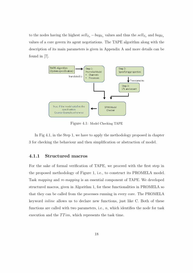
values of a core govern its agent negotiations. The TAPE algorithm along with the

description of its main parameters is given in Appendix A and more details can be

found in [7].

Figure 4.1: Model Checking TAPE

In Fig 4.1, in the Step 1, we have to apply the methodology proposed in chapter

3 for checking the behaviour and then simplification or abstraction of model.

4.1.1 Structured macros

For the sake of formal verification of TAPE, we proceed with the first step in

the proposed methodology of Figure 1, i.e., to construct its PROMELA model.

Task mapping and re-mapping is an essential component of TAPE. We developed

structured macros, given in Algorithm 1, for these functionalities in PROMELA so

that they can be called from the processes running in every core. The PROMELA

keyword inline allows us to declare new functions, just like C. Both of these

functions are called with two parameters, i.e., n, which identifies the node for task

execution and the TTim, which represents the task time.

18

Algorithm 1 Structured Macrosinline mapping(n,TTim) TTim:Task time{ 1: nown = nown + (TTim ∗ 1);2: freen = freen − (TTim ∗ 1);3: Tmn = Tmn + (TTim ∗ 4);4: usedn = usedn + (TTim ∗ 1);}

inline remapping(n,TTim){ 1: nown = nown + 1;2: rmp = rmp+ 1;3: dn = sellTn − buyTn; /*difference matrix */4: short mxm;5: if6: ::dn > mxm → mxm = dn; /*finding max(sell-buy)*/7: ::else→skip;8: fi;9: if /*mapping*/10: ::mxm == dn →11: nown = nown + (1 ∗ TTim);12: freen = freen − (1 ∗ TTim);13: usedn = usedn + (1 ∗ TTim);14: Tmn = Tmn + (4 ∗ TTim);15: fi;}

4.1.2 init: An initialization process

An initialization process, given in Algorithm 2, is used to initialize the data types

for all the variables used in our model and perform the initial task mapping. The

TAPE algorithm utilizes two normalizing factors, as and ab, to reflect temperature

effects on the values of buyTn and sellTn and four weights ωu,b, ωu,s, ωf,b and ωf,s

to reflect the effects of the variables usedn and freen on the values of buybase and

sellbase. All these variables are represented as real numbers in the TAPE algorithm

of [7]. However, SPIN does not support real or floating-point numbers and hence

these variables must be discretized as explained in the previous section. The ranges

19

of these variables can be found from the TAPE description [7]. For example, the

values of normalizing factors, as and ab, must be bounded in the interval (0, 1).

Due to the inability to express real numbers, we use integers in the interval [1, 9]

for assigning values to variables as and ab. In order to nullify the effect of this

discretization on the overall behavior of the model, we have to divide the equations

containing variables as and ab by 10 whenever they are used in the PROMELA

model. Similarly, based on the behavior of the TAPE model, integers in the interval

[0, 7] are used for the weight variables ωu,s, ωf,b and ωf,s and the interval [7, 14] for

the weight variable ωu,b. Therefore, in order to retain the behavior of the TAPE

model, we divide these variables by 7 whenever they are used in the PROMELA

models (See e.g., Lines 11 and 12 of Algorithm 2).

Algorithm 2 Initialization processinitialization process: init1: select(wus : 1..6);2: select(wfs : 1..6);3: select(wub : 7..13);4: select(wfb : 1..6);5: select(as : 1..9);6: select(ab : 1..9);7: for all nodes n8: freen = PUtotal/(rows ∗ col); For even distribution of Power units9: usedn = 0; initially no used power units10: Tmn = To; measured temperature is same as initial temperature initially11: sellbasen = (wus · usedn + wfs · freen)/712: buybasen = (wub · usedn + wfb · freen)/713: end formultiple task mapping is done randomly hereinstantiation of all agents and receiving processes are done here

20

4.2 Processes and channels

The grid of cores (or tiles) of TAPE can be modeled as a two dimensional array of

distributed nodes such that the TAPE algorithm runs on all these nodes concurrently.

Based on the proposed methodology, we represented the behavior of these nodes

using PROMELA processes and channels. We developed a generic node model so

that it can be repeatedly used to formally express any grid of arbitrary dimension.

A node is modeled using two main processes, i.e., the receiver process, given in

algorithm 3, that handles receiving values from the neighboring nodes and the

agent process, given in algorithm 4, that is mainly responsible for processing the

received values and then sharing them with the four neighbors of the node. The

usage of the separate receiving process ensures reliable exchange of information

as this way each node can receive information at any time irrespective of its main

agent being busy or not. We have used both sending and receiving channels that

are identified using the symbols ! and ? in the PROMELA model, respectively, for

every node.

Algorithm 3 Receiving Processn : identification of nodeproctype receiving(n,eastr,westr,northr,southr)1: if receiving2: ::eastr?buyTn, sellTn, time; → max(time, nown + 1)3: ::westr?buyTn, sellTn, time; → max(time, nown + 1)4: ::northr?buyTn, sellTn, time; → max(time, nown + 1)5: ::southr?buyTn, sellTn, time; → max(time, nown + 1)6: :: skip;7: fi;

21

Algorithm 4 Agent Processn : identification of nodeproctype agent(n,east,west,north,south)1: sellTn = sellbasen + (as · (Tmn − To))/10;2: buyTn = buybasen − (ab · (Tmn − To))/10;3: if4: :: (sellTn − buyTn)− (sellTn[i]− buyTn[i]) > τ →5: if6: ::freen > 0 →nown = nown + 1; freen = freen − 1; freen[i] = freen[i] + 17: ::else→8: nown = nown + 1; usedn = usedn − 1; freen[i] = freen[i] + 1;9: if10: ::tasktime > deadline →remapping(a, b, tasktime); Tmn = Tmn − 4;11: ::else→skip;12: fi13: fi14: ::else →skip;15: fi/*trading results in change of base buy/sell value*/16: if17: ::(buyTn! = lastbuyn) || (sellTn! = lastselln) →18: now = nown + 1; lastbuyn = buyTn; lastselln = sellTn19: east!buyTn, sellTn, nown;20: west!buyTn, sellTn, nown;21: north!buyTn, sellTn, nown;22: south!buyTn, sellTn, nown;23: :: skip;24: fi;

4.3 Temperature consideration

Finally, we also have to discretize the allowable increments and decrements for the

temperature variable Tm, which is assigned the value of the initial temperature

T0 = 30◦C at start-up. For this purpose, we assume that one or more energy units of

1 mJ are consumed during the execution of a particular task. Thus, the worst-case

temperature change that happens in one energy unit consumption can now be

22

calculated to be approximately equal to 4◦K using the relationship 1mJ/(CV ),

where C represents the heat capacity equal to 1.547 J.cm3K−1 for Silica and V

represents the volume of a core, which can be reasonably assumed to be equal to

1mm x1mm x150um.

4.4 Lamport Timestamps

In order to implement the Lamport timestamps algorithm, we increment the value

of nown whenever the node n gives a free power unit to one of its neighbors as a

result of agent negotiation or whenever the values sellTn and buyTn are updated or

whenever mapping, re-mapping (requires two events), sending or receiving takes

place.

It is worth mentioning that the above mentioned PROMELA model of TAPE

was finalized after numerous runs through the proposed methodology, i.e., it had to

go through deadlock checks and several stages of simplifications and optimizations.

We identified a deadlock in our first PROMELA model of TAPE, which occurred

because a single channel was used to model both receiving and sending, which in

turn lead to the possibility of missing the status update of a missing neighbor. To

avoid this situation, we have used two different processes per node to model sending

and receiving channels. Interestingly, this kind of a critical aspect, which prevents

the system to achieve stability, was not mentioned or caught by the simulation-

based analysis of TAPE that is reported in [7]. This point clearly indicates the

usefulness of the proposed approach and using formal methods for the verification

of distributed DTM schemes. Likewise, the above mentioned variable ranges had

to be finalized after many simplification and optimization stages so that the model

can be verified by the SPIN model checker without encountering the state-space

explosion problem. For 4x4 model the verification is not possible even trying alot

23

of abstractions and using bitstate, therefore verification is done for 3x3. Moreover,

we abstracted the DVFS considerations from the TAPE model since its presence

has nothing to do with the functional or timing verification and its removal results

in the simplification of the PROMELA model, which in turn leads to a reduced

state-space.

Due to the mathematical nature of the PROMELA models, merely the formal

specification of TAPE in PROMELA allowed us to catch many issues in the system.

For example, the exemplary runtime scenario of Figure 3 in [7] seems incorrect as

we were not able to recreate this scenario for our PROMELA model. Besides, these

small issues, we also have some useful information about the possible deadlocks in

the TAPE model as described above. These issues clearly indicate the shortcomings

of the simulation based analysis and are quite convincing to motivate the usage of

formal methods for the verification of distributed DTM systems.

24

Chapter 5

Verification Results

As our verification platform, we use the version 6.1.0 of the SPIN model checker

and version 1.0.3 of ispin along with the WINDOWS 7 Professional OS running on

i7-2600 processor, 3.4 GHz(8 CPUs) with 16 GB memory. The verification is done

for a 3x3 grid of nodes (cores) with all of them running the processes and channels

described in the previous section. Thus, the whole model contains 18 processes and

350 lines of code and produces a comparatively huge state-space. The verification

utility BITSTATE is used for verification purposes in SPIN since it uses 2808 Mb

of space while allowing to work with up to 4.8 · 106 states and thus suffices for the

given problem.

The most interesting functional characteristic to be verified in the context of

TAPE is to ensure that the agent trading is always able to achieve a stable power

budget distribution. For instance, it needs to be shown that no circular trading

loops emerge where power budget is continuously traded preventing the system

from stabilizing. Another possibility is that localized minima form which act as

a barrier that prevents power budget from propagating. As a result, cores on

one side of the barrier would no longer be able to obtain power budget even if

it were available globally, and new tasks would be mapped to the other side of

the barrier where power budget has accumulated. If such a scenario is possible,

it would result in high temperatures and frequent re-mapping inside the region

with the power budget not allowing the system to stabilize even though a global

stable configuration would be possible. This kind of instability can be ensured to

Table 5.1: Statistics of all the 12 properties verified where p0001 is related to node (0,0) and(0,1) and so on

SPIN 6.1.0 – 4 May 2011All neighboring tiles/regions relations verified

Transitions States stored Memory Usage(MB) Verification Time(sec)Horizontal Relations

Property 1(p0001)

25244478 4786929 2808.8 80.9

Property 2(p0102)

25295692 4787223 2808.808 81.3

Property 3(p1011)

24991059 4755543 2803.658 83.5

Property 4(p1112)

25193755 4772741 2816.247 82.7

Property 5(p2021)

25244421 4786926 2808.808 84.1

Property 6(p2122)

25244421 4786926 2808.808 83.9

Vertical RelationsProperty 7(p0010)

24672155 4721204 2564.477 76

Property 8(p1020)

24947360 4751100 2564.477 76.9

Property 9(p0111)

25055780 4760200 2564.477 76.9

Property 10(p1121)

25097601 4764453 2564.477 77.3

Property 11(p0212)

24982388 4749616 2564.477 76.8

Property 12(p1222)

25114849 4759582 2564.477 77.3

not occur by verifying that “Eventually the sell-buy value between any two adjacent

tiles must be some small value”. We have to verify 12 such properties so that all

possible node pairs are covered. For example, this property can be expressed for

nodes 00 and 01, of a 3x3 grid as:

[](<> ((sell T[0].vector[0] - buy T[0].vector[0]) -

(sell T[0].vector[1] - buy T[0].vector[1])<4 ))

In a similar way, we expressed and verified the rest of the 11 properties as well.

26

On average, each one of these property verifications required around 80-100 seconds

and 2808 Megabytes of memory and the corresponding finite-state machine had

around 50,00,000 states and 2,50,00,000 state transitions. No unreachable code

was detected during the analysis.

Table 5.2: Effect of as(Total Power units:128, Tasks:10, ab:2/10, wus:2/7, wfs:2/7, wub:8/7,wfb:2/7)

as Events to Stability Tm(max), To = 30oC0.1 20 380.2 20 380.3 21 380.4 21 380.5 22 380.6 22 380.7 29 380.8 67300 380.9 63932 38

Table 5.3: Effect of ab(Total Power units:128, Tasks:10, as:2/10, wus:2/7, wfs:2/7, wub:8/7,wfb:2/7)

ab Events to Stability Tm(max), To=30oC0.1 20 380.2 12 380.3 12 380.4 21 380.5 22 380.6 22 380.7 22 380.8 65322 380.9 64282 38

For timing verification, we formally executed the PROMELA model of the

previous section and observed the effect of number of tasks and the values of

variables as and ab, on the number of events and temperature. The values of the

global list now are observed for acquiring the information about the number of

27

events and the overall results of the timing verification are summarized in Tables

2-4. All these results have been observed for ωu,s=2, ωf,b=2, ωf,s=2 and ωu,b=8.

From the Tables 5.2 and 5.3, it is clearly observed that the algorithm reaches

the stable state, where power is evenly distributed and no redundant trading of

power units take place, only when

as + ab < 1

and thus results in stability. This is the condition found, after which the verification

is successful, under the variable ranges mentioned in [7]

The statistics for all twelve verified properties are given in Table 5.1. From

these statistics, complexity of verification process and huge nature of state space

can be observed.

According to TAPE [7], the range of both as and ab is (0,1). For the first time,

when I go for verification, the model fails to satisfy the specified properties. Then I

have gone through repeated simulations by keeping all variables constant except one

to see the possible effect on the stability. The initial temperature considered here

is 30oC and changes on the events to stability are observed for a specific number

of tasks to be executed. Here No. of tasks considered is 10. The simulations are

done till 250,000 simulation steps and then values are recorded. The No. of events

must be some limited small value if system results in stability. From the above two

tables for as and ab, it is clearly observed that the algorithm reaches the stable

state, where power is evenly distributed and no redundant trading of power units

take place, only when

as + ab < 1

and thus results in stability. After this observation and appropriate changes for

this condition, all the specified properties are verified easily and hence the TAPE

28

model’s stability is ensured. The statistics of all these verified properties are given

in table 5.1. The measured temperature doesn’t have variations recorded because

the No. of tasks is constant.

Table 5.4: Effect of Tasks (Total Power units:128, as:2/10, ab:2/10, wus:2/7, wfs:2/7, wub:8/7,wfb:1/7)

Tasks Events to Stability Tm(max) Tasks Re-mapped1 8 34 02 9 34 03 9 34 04 10 34 05 10 34 010 14 38 015 28 42 020 40 42 025 53 42 030 59 46 035 23 46 040 43 50 045 35 54 050 32 54 055 30 86 160 67 86 6

Table 5.4 shows that No. of events increase when the number of tasks increase.

Task remapping is done only in the most severe cases, when the No. of free power

units with neighbor differs too much or almost all the free power units are consumed.

The distinguishing characteristic of the analysis presented in this section is its

exhaustive nature, which cannot be attained by the traditional simulation due to

the large number of possibilities. It is also important to note that the verification

process is completely automatic and the human interaction is only required for

debugging purposes.

29

Chapter 6

Conclusions

6.1 Summary

The report presents a formal verification methodology for distributed DTM systems.

The proposed method mainly utilizes the SPIN model checker and Lamport time-

stamps algorithm to verify both functional and timing properties. To the best of our

knowledge, this is the first formal verification approach for distributed DTM systems.

For illustration purposes, the paper presents the successful formal verification of

TAPE, which is a recently proposed agent-based DTM. The advantage of TAPE

over others is its agent based and distributed approach having no central control

instance unlike others which during a lot of negotiations itself becomes a main

point of failure. Only the behavior of algorithm/protocol can be modelled with

some simplifications and abstractions due to memory constraints such that the

basic behavior remains same. This case study clearly indicates the applicability of

the proposed methods to verify real-world distributed DTM approaches. Likewise,

the proposed methodology can be used to verify other prominent distributed DTM

schemes.

6.2 Future Work

This model of TAPE is verified using the BITSTATE analysis method of SPIN in

order to reduce the memory requirements as otherwise the resources are completely

30

utilized resulting in the out of memory problem. In case of the availability of better

computational resources in terms of memory and processing power, we may use the

standard verification methods of SPIN as this choice would provide more confidence

on the analysis results due to its exhaustive nature.

A major limitation of model checking observed in this thesis is the state-space

explosion. This is the reason that we could not verify more than a 9 node/core

DTM system. In order to alleviate this problem, higher-order-logic theorem proving

may be used for the verification of DTM schemes. However, this would be done at

the cost of a considerable human interaction.

31

References

[1] SPIN V2 Update 2.6 (16 July 1995). http://spinroot.com/spin/Doc/V2.

Updates, 2012.

[2] J. Abrial. Faultless systems: Yes we can! IEEE Computer, 42(9):30–36, 2009.

[3] C. Baier and J.P. Katoen. Principles of Model Checking. MIT Press, YEAR

= 2008,.

[4] S. Borkar. Thousand core chips: a technology perspective. In Design Automa-

tion Conference, pages 746–749. ACM, 2007.

[5] J. Donald and M. Martonosi. Techniques for multicore thermal management:

Classification and new exploration. In Symposium on Computer Architecture,

pages 78–88. IEEE Computer Society, 2006.

[6] D. Dunn. Intel delays montecito in roadmap shakeup. EE Times, Manufac-

turing/Packaging, Oct. 27, 2005.

[7] T. Ebi, M. Faruque, and J. Henkel. Tape: Thermal-aware agent-based power

econom multi/many-core architectures. In Computer-Aided Design, pages 302

–309, 2009.

[8] Y. Ge, P. Malani, and Q. Qiu. Distributed task migration for thermal man-

agement in many-core systems. In Design Automation Conference, pages 579

–584, 2010.

[9] G.J. Holzmann. Design and validation of computer protocols. Prentice-Hall,

Inc., 1991.

32

[10] G.J. Holzmann. The model checker SPIN. IEEE Transactions on Software

Engineering, 23(5):279–295, 1997.

[11] ITRS. http://www.itrs.net, 2012.

[12] M. Kadin, S. Reda, and A. Uht. Central vs. distributed dynamic thermal

management for multi-core processors: which one is better? In Great Lakes

symposium on VLSI, pages 137–140, 2009.

[13] J.A. Kumar and S. Vasudevan. Verifying dynamic power management schemes

using statistical model checking. In Asia and South Pacific Design Automation

Conference, pages 579–584. IEEE, 2012.

[14] L. Lamport. Time, clocks, and the ordering of events in a distributed system.

Commun. ACM, 21(7):558–565, 1978.

[15] A. Lungu, P. Bose, D.J. Sorin, S. German, and G. Janssen. Multicore power

management: Ensuring robustness via early-stage formal verification. In

Formal Methods and Models for Co-Design, pages 78 –87, 2009.

[16] G. Norman, D. Parker, M. Kwiatkowska, S. Shukla, and R. Gupta. Using

probabilistic model checking for dynamic power management. Formal Aspects

of Computing, Springer-Verlag, 17(2):160–176, 2005.

[17] S.K. Shukla and R.K. Gupta. A model checking approach to evaluating system

level dynamic power management policies for embedded systems. In High-Level

Design Validation and Test Workshop, pages 53–57. IEEE Computer Society,

2001.

[18] K. Skadron. ”temperature-aware microarchitecture: Extended discussion

and results”. Univ. of Virginia, Dept. of Computer Science, Tech. report

CS-2003-08, Charlottesville, 2003.

33

Appendix A

TAPE Algorithm

Algorithm: Thermal-aware Agent-based power economy for DTMsellbasen : Base sell value of a tile n at time t

buybasen : Base buy value of a tile n at time t

Tn: Temperature of a tile n at time t

sellTn: Sell value of a tile n at a temperature Tn

buyTn: Buy value of a tile n at a temperature Tn

Nn: Set of all the neighboring tiles of tile n

lastbuy, lastsell: Last buy/sell values of a tile n sent to all i ∈ Nbuy[N ], sell[N ]: List of buy/sell values of neighboring tiles stored in n

freen: Free power units of tile n

usedn: Power units used for running tasks on tile n

tj : Tasks running on tile n at time t

τn: sell threshold of tile n

1: loop2: for all tiles n in parallel do3: at every time interval ∆nt do // Calculate base sell value4: sellbasen ← (wu,s · usedn + wf,s · freen)5: buybasen ← (wu,b ·usedn−wf,b · freen) // The temperature increase may happen due to change

in PE activity. Modify buy/sell value6: sellTn ← sellbasen + as·(Tmn − To) +7: buyTn ← buybasen - ab·(Tmn − To)8: if ∃i ∈ Nn : ((sellTn − buyTn )− (sell[i]− buy[i]) > τn then9: if any free power units are left then

10: decrement freen11: else12: apply DVFS on n to get more free power units13: decrement usedn14: if the task does not meet the given deadline as DVFS is used then15: (re-)mapping needs to be invoked16: else17: graceful performance degradation if allowed18: end if19: end if20: increment freei21: end if22: if buyTn 6= lastbuy or sellTn 6= lastsell then23: send buyTn to all i ∈ N24: send sellTn to all i ∈ N25: lastbuy ← buyTn

26: lastsell ← sellTn

27: end if // This procedure will propagate until a stable state is reached.28: end at29: if received updated buy/sell values from any l ∈ Nn then30: update buy[l], sell[l]31: end if32: if new task mapped to n requiring k power units then33: freen ← freen − k34: apply DVFS to PE on tile n35: usedn ← usedn + k36: end if37: end for

38: end loop

34