FORMAL DESIGN OF ASYNCHRONOUS FAULT DETECTION AND ... · FORMAL DESIGN OF ASYNCHRONOUS FAULT...
33
Logical Methods in Computer Science Vol. 11(4:4)2015, pp. 1–33 www.lmcs-online.org Submitted Jan. 13, 2014 Published Nov. 4, 2015 FORMAL DESIGN OF ASYNCHRONOUS FAULT DETECTION AND IDENTIFICATION COMPONENTS USING TEMPORAL EPISTEMIC LOGIC MARCO BOZZANO, ALESSANDRO CIMATTI, MARCO GARIO, AND STEFANO TONETTA Fondazione Bruno Kessler, Trento, Italy e-mail address : {bozzano, cimatti, gario, tonettas}@fbk.eu Abstract. Autonomous critical systems, such as satellites and space rovers, must be able to detect the occurrence of faults in order to ensure correct operation. This task is carried out by Fault Detection and Identification (FDI) components, that are embedded in those systems and are in charge of detecting faults in an automated and timely manner by reading data from sensors and triggering predefined alarms. The design of effective FDI components is an extremely hard problem, also due to the lack of a complete theoretical foundation, and of precise specification and validation techniques. In this paper, we present the first formal approach to the design of FDI components for discrete event systems, both in a synchronous and asynchronous setting. We propose a logical language for the specification of FDI requirements that accounts for a wide class of practical cases, and includes novel aspects such as maximality and trace-diagnosability. The language is equipped with a clear semantics based on temporal epistemic logic, and is proved to enjoy suitable properties. We discuss how to validate the requirements and how to verify that a given FDI component satisfies them. We propose an algorithm for the synthesis of correct-by-construction FDI components, and report on the applicability of the design approach on an industrial case-study coming from aerospace. 1. Introduction The operation of complex critical systems (e.g., trains, satellites, cars) increasingly relies on the ability to detect when and which faults occur during operation. This function, called Fault Detection and Identification (FDI), provides information that is vital to drive the containment of faults and their recovery. This is especially true for fail-operational systems, where the occurrence of faults should not compromise the ability to carry on critical functions, as opposed to fail-safe systems, where faults are typically handled by going to a safe state. FDI is often carried out by dedicated modules, called FDI components, running 2012 ACM CCS: [Theory of computation]: Logic—Logic and verification — Verification by model checking; [Computing methodologies]: Artificial intelligence—Knowledge representation and reasoning— Temporal reasoning; Artificial intelligence—Reasoning about belief and knowledge / Causal reasoning and diagnostics; [Hardware]: Robustness—Fault tolerance / Hardware reliability. Key words and phrases: Fault Detection and Identification; Diagnoser Synthesis; Model Checking; Tem- poral Epistemic Logic. LOGICAL METHODS IN COMPUTER SCIENCE DOI:10.2168/LMCS-11(4:4)2015 c M. Bozzano, A. Cimatti, M. Gario, and S. Tonetta CC Creative Commons
Transcript of FORMAL DESIGN OF ASYNCHRONOUS FAULT DETECTION AND ... · FORMAL DESIGN OF ASYNCHRONOUS FAULT...
Logical Methods in Computer ScienceVol. 11(4:4)2015, pp. 1–33www.lmcs-online.org
Submitted Jan. 13, 2014Published Nov. 4, 2015
FORMAL DESIGN OF ASYNCHRONOUS
FAULT DETECTION AND IDENTIFICATION COMPONENTS
USING TEMPORAL EPISTEMIC LOGIC
MARCO BOZZANO, ALESSANDRO CIMATTI, MARCO GARIO, AND STEFANO TONETTA
Fondazione Bruno Kessler, Trento, Italye-mail address: {bozzano, cimatti, gario, tonettas}@fbk.eu
Abstract. Autonomous critical systems, such as satellites and space rovers, must beable to detect the occurrence of faults in order to ensure correct operation. This task iscarried out by Fault Detection and Identification (FDI) components, that are embeddedin those systems and are in charge of detecting faults in an automated and timely mannerby reading data from sensors and triggering predefined alarms.
The design of effective FDI components is an extremely hard problem, also due tothe lack of a complete theoretical foundation, and of precise specification and validationtechniques.
In this paper, we present the first formal approach to the design of FDI componentsfor discrete event systems, both in a synchronous and asynchronous setting. We proposea logical language for the specification of FDI requirements that accounts for a wide classof practical cases, and includes novel aspects such as maximality and trace-diagnosability.The language is equipped with a clear semantics based on temporal epistemic logic, andis proved to enjoy suitable properties. We discuss how to validate the requirements andhow to verify that a given FDI component satisfies them. We propose an algorithm forthe synthesis of correct-by-construction FDI components, and report on the applicabilityof the design approach on an industrial case-study coming from aerospace.
1. Introduction
The operation of complex critical systems (e.g., trains, satellites, cars) increasingly relieson the ability to detect when and which faults occur during operation. This function,called Fault Detection and Identification (FDI), provides information that is vital to drivethe containment of faults and their recovery. This is especially true for fail-operationalsystems, where the occurrence of faults should not compromise the ability to carry on criticalfunctions, as opposed to fail-safe systems, where faults are typically handled by going to asafe state. FDI is often carried out by dedicated modules, called FDI components, running
2012 ACM CCS: [Theory of computation]: Logic—Logic and verification—Verification by modelchecking; [Computing methodologies]: Artificial intelligence—Knowledge representation and reasoning—Temporal reasoning; Artificial intelligence—Reasoning about belief and knowledge /Causal reasoning anddiagnostics; [Hardware]: Robustness—Fault tolerance /Hardware reliability.
Key words and phrases: Fault Detection and Identification; Diagnoser Synthesis; Model Checking; Tem-poral Epistemic Logic.
LOGICAL METHODSl IN COMPUTER SCIENCE DOI:10.2168/LMCS-11(4:4)2015
c© M. Bozzano, A. Cimatti, M. Gario, and S. TonettaCC© Creative Commons
2 M. BOZZANO, A. CIMATTI, M. GARIO, AND S. TONETTA
in parallel with the system. An FDI component, hereafter also referred to as a diagnoser,processes sequences of observations, made available by predefined sensors, and is requiredto trigger a set of predefined alarms in a timely and accurate manner. The alarms are thenused by recovery modules to guarantee the survival of the system without requiring externalcontrol. Faults are often not directly observable. Their occurrence can only be inferred byobserving the effects that they have on the observable parts of the system. Moreover, faultsmay have complex dynamics, and may interact with each other in complex ways.
For these reasons, the design of FDI components is a very challenging task, and also apractical problem, as witnessed by multiple Invitations To Tender issued by the EuropeanSpace Agency [Eur10, Eur11, Eur13]. The current methodologies lack a comprehensivetheoretical foundation, and do not provide clear and effective specification and validationtechniques and tools. Most approaches asses the quality of an FDI component based onsimulation and quantitative analysis [FKN+10], that do not start from a specification ofthe behavior the the FDI needs to satisfy. This leads to a uniform treatment of all faults,while in general some faults are more important then others, and in many cases we are notinterested in the specific fault characteristics but only to know that the fault occurred ina given part of the system (isolation). As a consequence, the design often results in veryconservative assumptions, so that the overall system features sub-optimal behaviors, and itis not trusted during critical phases.
The goal of this paper is to propose a formal foundation to support the design ofFDI components. We provide a way to specify FDI components, and cover the followingproblems: (i) validation of an FDI component specification, (ii) verification of a given FDIcomponent with respect to a given specification, and (iii) automated synthesis of an FDIcomponent from a given specification.
The specification of an FDI component is tackled by introducing a pattern-based lan-guage. Intuitively, an FDI component is specified by stating the observable signals (theinputs of the FDI component), the desired alarms (in terms of the unobservable state), andby defining the relation between the two. The language supports various forms of delay (ex-act, finite, bounded) between the occurrence of faults and the raising of the correspondingalarm. The patterns are given a formal semantics expressed in terms of epistemic temporallogic [HV89], where the knowledge operator is used to express the certainty of a condition,based on the available observations. The formalization encodes properties such as alarmcorrectness and alarm completeness. Correctness states that whenever an alarm is raised bythe FDI component, then its associated triggering condition did occur; completeness statesthat if an alarm is not raised, then either the associated condition did not occur, or it wouldhave been impossible to detect it, given the available observations. Moreover, we preciselycharacterize two aspects that are important for the specification of FDI requirements. Thefirst one is the diagnosability of the plant, i.e., whether the sensors convey enough informa-tion to detect the required conditions. We explain how to deal with non-diagnosable plantsby introducing a more fine-grained concept of trace diagnosability, where diagnosability islocalized to individual traces. Most of the state of the art focuses on the fact that the systemis diagnosable for any execution. However, in practice, this is rarely the case, since usuallythe plant is diagnosable in many situations but not in all of them. The classic example isthe one of a burnt light-bulb, of which we cannot say anything until we try to turn it on.In this case, we would like to build a diagnoser that can raise the alarm whenever thereis no ambiguity on whether the light bulb is burnt. Therefore, we introduce the concept

FORMAL DESIGN OF ASYNCHRONOUS FDI USING TEMPORAL EPISTEMIC LOGIC 3
of trace diagnosability, intuitively accepting the fact that the plant might not always bediagnosable.
The second important concept that we introduce is maximality. A diagnoser is maximalif it is able to raise an alarm as soon as and whenever possible. This, in particular, meansthat in all traces that are diagnosable, a maximal diagnoser needs to raise the alarm.
The approach provides a full account of synchronous and asynchronous perfect-recallsemantics for the epistemic operator. We show that the specification language correctlycaptures the formal semantics and we clearly define the relation between diagnosability,maximality and correctness.
Within our setting, the validation of a diagnoser specification is reduced to validitychecking in temporal epistemic logic, while the verification of a given diagnoser is mappedto model checking for a temporal epistemic logic. As for synthesis, we propose an algorithmthat is proved to generate correct-by-construction diagnosers.
From the practical standpoint, the applicability of the design approach has been demon-strated on two projects funded by the European Space Agency [AUT, FAM]. The paper ac-tually provides the conceptual foundation underlying a design tool-set [ANY+12, BBC+14a,BBC+14b], which has been applied to the specification, verification and synthesis of an FDIcomponent for a satellite.
Finally, please note the deep difference between the design of FDI components and mostdiagnosis [dKK04] approaches. In most settings, diagnosis systems can benefit from powerfulcomputing platforms. Partial diagnoses are typically acceptable, and can be complementedby further (post-mortem) inspections. This is typical of approaches that rely on logicalreasoning engines (e.g., SAT solvers [GARK07]). Other approaches [HD05, SSL+95, Sch04]rely on knowledge compilation to reduce the on-line complexity. An FDI component, onthe contrary, runs on-board (as part of the on-line control strategy), and is subject torestrictions of various nature, such as timing and computation power. FDI design thusrequires a deeper theory, which accounts for the issues of delay in raising the alarms, tracediagnosability, and maximality. Moreover, it becomes crucial to be able to verify and certifythe effectiveness of the system, since it might not be possible to change it after deployment.
This paper is structured as follows. Section 2 provides some introductory backgroundand introduces our running example. Section 3 formalizes the notion of FDI. Section 4presents the specification language. In Section 5, we discuss how to validate the require-ments, and how to verify an FDI component with respect to the requirements. In Section 6,we present an algorithm for the synthesis of correct-by-construction FDI components. Theresults of evaluating our approach in an industrial setting are presented in Section 7. Sec-tion 8 compares our work with previous related works. In Section 9, we draw some conclu-sions and outline the directions for future work.
2. Background
2.1. Labeled Transition Systems. In order to model the plant and the FDI, we use asymbolic representation of Labeled Transition Systems (LTS). Control locations and dataare represented by variables, while sets of states and transitions are represented by formulas,and transitions are labeled with explicit events.
Given a set of variables X and a (finite) domain U of values, an assignment to X is amapping from the set X to the set U . We use Σ(X) to denote the set of assignments to X.

4 M. BOZZANO, A. CIMATTI, M. GARIO, AND S. TONETTA
Given an assignment a ∈ Σ(X) and X1 ⊆ X, we use a|X1to denote the projection of a over
X1. We use F(X) to denote the set of propositional formulas over X.
Definition 2.1 (LTS). A Labeled Transition System is a tuple S = 〈V,E, I,T 〉, where:
• V is the set of state variables;• E is the set of events;• I ∈ F(V ) is a formula over V defining the initial states;• T : E → F(V ∪ V ′) maps an event e ∈ E to a formula over V and V ′ defining thetransition relation for e (with V ′ being the next version of the state variables).
A state s is an assignment to the state variables V (i.e., s ∈ Σ(V )). We denote by s′ thecorresponding assignment to V ′. A transition labeled with e is a pair of states 〈s, s′〉 suchthat s, s′ |= T (e). A trace of S is a sequence σ = s0, e0, s1, e1, s2, . . . alternating states andevent such that s0 satisfies I and, for each k ≥ 0, 〈sk, sk+1〉 satisfies T (ek). Note that weconsider infinite traces only, and w.l.o.g. we assume the system to be dead-lock free. Givenσ = s0, e0, s1, e1, s2, . . . and an integer k ≥ 0, we denote by σk the finite prefix s0, e0, . . . , skof σ containing the first k+1 states. We denote by σ[k] the k+1-th state sk. We say thats is reachable in S iff there exists a trace σ of S such that s = σ[k] for some k ≥ 0.
We say that S is deterministic iff:
(i) there is one initial state (i.e., there exists a state s such that s |= I and, for all t, ift |= I, then s = t);
(ii) for every reachable state s, for every event e, there is one successor (i.e., there exists s′
such that 〈s, s′〉 |= T (e) and, for all t′, if 〈s, t′〉 |= T (e), then s′ = t′).
Definition 2.2 (Synchronous Product). Let
S1 = 〈V 1, E1, I1,T 1〉 and S2 = 〈V 2, E2, I2,T 2〉
be two transition systems with E1 = E2 = E. We define the synchronous product S1×S2 asthe transition system 〈V 1 ∪ V 2, E, I1 ∧ I2,T 〉 where, for every e ∈ E, T (e) = T 1(e)∧T 2(e).Every state s of S1 × S2 can be considered as the product s1 × s2 such that s1 = s|V 1 is
a state of S1 and s2 = s|V 2 is a state of S2. Similarly, every trace σ of S1 × S2 can be
considered as the product σ1 × σ2 where σ1 is a trace of S1 and σ2 is a trace of S2.
Definition 2.3 (Asynchronous Product). Let
S1 = 〈V 1, E1, I1,T 1〉 and S2 = 〈V 2, E2, I2,T 2〉
be two transition systems. We define the asynchronous product S1 ⊗ S2 as the transitionsystem 〈V 1 ∪ V 2, E1 ∪E2, I1 ∧ I2,T 〉 where:
• for every e ∈ E1 \E2, T (e) = T 1(e) ∧ frame(V 2 \ V 1).• for every e ∈ E2 \E1, T (e) = T 2(e) ∧ frame(V 1 \ V 2).• for every e ∈ E1 ∩E2, T (e) = T 1(e) ∧ T 2(e).
where frame(X) stands for∧
x∈X x′ = x and is used to represent the fact that while one
transition system moves on a local event, the other transition system does not change itslocal state variables. Every state s of S1 ⊗ S2 can be considered as the product s1 ⊗ s2
such that s1 = s|V 1 is a state of S1 and s2 = s|V 2 is a state of S2. If either S1 or S2
is deterministic, also every trace σ of S1 ⊗ S2 can be considered as the product σ1 ⊗ σ2
where σ1 is a trace of S1 and σ2 is a trace of S2 (more in general, the product of two tracesproduces a set of traces due to different possible interleavings).

FORMAL DESIGN OF ASYNCHRONOUS FDI USING TEMPORAL EPISTEMIC LOGIC 5
In general, composing two systems can reduce the behaviors of each system and in-troduce deadlocks. However, given two systems that do not share any state variable (e.g.,the diagnoser and the plant), if one of the systems is deterministic (the diagnoser) then itcannot alter the behavior of the second (the plant).
Notice that the synchronous product coincides with the asynchronous case when thetwo sets of events coincide.
2.2. Linear Temporal Logic. We now present a Linear Temporal Logic extended withpast operators [Pnu77, LMS02, LPZ85], in the following simply referred to as LTL. Aformula in LTL over variables V and events E is defined as
β ::= p | e | β ∧ β | ¬β| Oβ | Y β | βSβ | Gβ | Fβ | Xβ | βUβ
where p is a predicate over F(V ) and e ∈ E. Intuitively, p are the propositions over thestate of the LTS, while e represents an event.
Given a trace σ = s0, e0, s1, e1, s2, . . ., the semantics of LTL is defined as follows:
- σ, i |= p iff si |= p- σ, i |= e iff ei = e- σ, i |= β1 ∧ β2 iff σ, i |= β1 and σ, i |= β2- σ, i |= ¬β iff σ, i 6|= β- Once: σ, i |= Oβ iff ∃j ≤ i. σ, j |= β- Yesterday: σ, i |= Y β iff i > 0 and σ, i− 1 |= β- Since: σ, i |= β1Sβ2 iff there exists j ≤ i such that σ, j |= β2 and for all k, j < k ≤ i,σ, k |= β1
- Finally: σ, i |= Fβ iff ∃j ≥ i. σ, j |= β- Globally: σ, i |= Gβ iff ∀j ≥ i. σ, j |= β- Next: σ, i |= Xβ iff σ, i+ 1 |= β- Until: σ, i |= β1Uβ2 iff there exists j ≥ i such that σ, j |= β2 and for all k, i ≤ k < j,σ, k |= β1.
Given an LTS S = 〈V,E, I,T 〉, S |= β iff for every trace σ of S, σ, 0 |= β.Notice that Y β is always false in the initial state, and that we use a reflexive semantics
for the operators U , F , G, S and O. We use the abbreviations Y nβ = Y Y n−1β (withY 0β = β), O≤nβ = β ∨ Y β ∨ · · · ∨ Y nβ and F≤nβ = β ∨Xβ ∨ · · · ∨Xnβ.
2.3. Partial Observability. A partially observable LTS is an LTS S = 〈V,E, I,T 〉 ex-tended with a set Eo ⊆ E of observable events.
We consider here only observations on events. In practice, observation on states arecommon and relevant. However, dealing with them in the asynchronous setting makes theformalism less clear. Therefore, we limit ourselves to observations on events and wheneverobservations on state variables are needed, such as sensor readings, we incorporate them inthe events as done in [SSL+96].
The observable part of the prefix σk of a trace σ is defined recursively as follows:obs(σ0) = ǫ (empty sequence); if e ∈ Eo, then obs(σk, e, s) = obs(σk), e; if e 6∈ Eo, thenobs(σk, e, s) = obs(σk).
Definition 2.4 (Observation Point). We say that i is an observation point for σ, denotedby ObsPoint(σ, i), iff the last event of σi is observable, i.e., iff σi = σ′, e, s for some σ′, e, sand e ∈ Eo.

6 M. BOZZANO, A. CIMATTI, M. GARIO, AND S. TONETTA
The notion of two traces being observationally equivalent requires that the two tracesend both or neither in an observation point. This captures the idea that a trace ending in anobservation point can be distinguished from the same trace extended with local unobservablesteps. In other terms, an observer can distinguish the instant in which it is observing andan instant right after.
Definition 2.5 (Observational Equivalence). We say that ((σ1, i), (σ2, j)) ∈ ObsEq if andonly if:
- ObsPoint(σ1, i) iff ObsPoint(σ2, j), and
- obs(σi1) = obs(σj2).
2.4. Temporal Epistemic Logic. Epistemic logic has been used to describe and reasonabout knowledge of agents and processes. There are several ways of extending epistemiclogic with temporal operators. We use the logic KL1 [HV89], extended with past operators.A formula in KL1 is defined as
β ::= p | e | β ∧ β | ¬β| Oβ | Y β | βSβ | Fβ | Xβ | βUβ | Gβ | Kβ
KL1 can be seen as extension of LTL with past operators, with the addition of theepistemic operator K. The intuitive semantics of Kβ is that the reasoner knows that βholds in a state of a trace σ, by using only the observable information. This means thatKβ holds iff β holds in all situations that are observationally equivalent. Therefore, whilein LTL the interpretation of a formula is local to a single trace, in KL1 the semantics ofthe K operator quantifies over the set of indistinguishable traces. Given a trace σ1 of apartially observable LTS, the semantics of K is formally defined as:
σ1, i |= Kβ iff ∀σ2,∀j. if ((σ1, i), (σ2, j)) ∈ ObsEq then σ2, j |= β.
Kβ holds at time i in a trace σ1 iff β holds in all traces that are observationallyequivalent to σ1 up to time i. Note that, due to the asynchronous nature of the observations,two traces of different length might lead to the same observable trace. This definitionimplicitly forces perfect-recall in the semantics of the epistemic operator, since we definethe epistemic equivalence between traces and not between states.
In many situations, we are interested in considering formulas only at observation points.We do so by introducing the following abbreviation.
Definition 2.6 (Observed). If Eo is the set of observable events, given a formula φ, we use
xφy(read “Observed φ”) as abbreviation for φ ∧ Y
∨e∈Eo
e.
2.5. Running Example. The Battery Sensor System (BSS) (Figure 1) will be our runningexample. The BSS provides a redundant reading of the sensors to a device. Internal batteriesprovide backup in case of failure of the external power supply. The safety of the systemdepends on both of the sensors providing a correct reading. The system can work in threedifferent operational modes: Primary, Secondary 1 and Secondary 2. In Primary mode,each sensor is powered by the corresponding battery. In the Secondary modes, instead,both sensors are powered by the same battery; e.g., during Secondary 1, both Sensor 1 andSensor 2 are powered by Battery 1. The Secondary modes are used to keep the systemoperational in case of faults. However, in the secondary modes, the battery in use willdischarge faster.

FORMAL DESIGN OF ASYNCHRONOUS FDI USING TEMPORAL EPISTEMIC LOGIC 7
Generator 1
Generator 2
Battery 1
Battery 2
Sensor 1
Sensor 2
Switch
Generator IN
Generator IN
Sensor OUT
Sensor OUT
Mode Selector
Device
Power
Control
Data
Figure 1. Running Example (Battery Sensor System)
We consider two possible recovery actions: i) Switch Mode, or ii) Replace the Battery-Sensor Block (the dotted block in Figure 1). In order to decide which recovery to apply, weare going to define a set of requirements connecting the faults to alarms. The faults andobservable information of the system are shown in Figure 2.
This example is particularly interesting because we can define two sources of delay:the batteries, and the device resilience to wrong inputs. The batteries provide a buffer forsupplying power to the sensors. The size of this buffer is determined by the capacity of thebattery, the initial charge, and the discharge rate. For the device, we assume that two validsensor readings are required for optimal behavior, however, we can work in degraded modewith only one valid reading for a limited amount of time. The device will stop working ifboth sensors are providing invalid readings, or if one sensor has been providing an invalidreading for too long.
Both a synchronous and asynchronous version of this model are possible. In the asyn-chronous model, we have an event for each possible combination of observations (e.g., “ModePrimary & Battery 1 Low”). In the synchronous model, we also have an additional observ-able event (tick) that represents the passing of time in the absence of any observable event.This event forces the synchronization of the plant with the diagnoser. The key differencebetween the synchronous and asynchronous setting is the amount of information that wecan infer in this particular case. For example, if we know the initial charge level of a battery,and we know its discharge rate (given by the operational mode), then at each point in timewe can infer the current charge of the battery. By comparing our expectation with theavailable information, we can detect when something is not behaving as expected. Unfortu-nately, there are practical settings in which the assumption of synchronicity is not realistic.Therefore, our approach accounts for both the synchronous and asynchronous models.
Observables Possible ValuesMode Primary, Secondary 1, Secondary 2Battery Level {1, 2} High, Mid, LowSensors Delta Zero, Non-Zero (|S1.Out− S2.Out| = 0)Device Status On, Off
Component FaultsGenerator Off (G1Off , G2Off )Battery Leak (B1Leak, B2Leak)Sensor Wrong Output (S1WO, S2WO)
Figure 2. Observables and Faults Summary

8 M. BOZZANO, A. CIMATTI, M. GARIO, AND S. TONETTA
To provide a better understanding of how the running example behaves, we providethe LTS of each of the components. Figure 3 shows the LTS of the generator and switch.We assume that the only way the generator can turn off is if a fault event occurs, thus themodel of the generator is rather simple. Also the switch features a rather simple model,where the labels toS1 and toS2 are defined as:
• toS1: Mode=Secondary1 ∧ Battery1.Double ∧ Battery2.Offline• toS1: Mode=Secondary2 ∧ Battery1.Offline ∧ Battery1.Double
thus they drive the change in operational mode of the batteries.
Onstart OffFault & Off PrimarySecondary
1Secondary
2
start
toS1 toS2
Figure 3. Generator (Left) and Switch (Right) LTS
Figure 4 shows two slightly more complex components: the sensor and the device.The sensor periodically outputs a good or a bad reading depending on the state it is in.Notice that the transition from a good to a bad state can occur either because of a fault(Wrong Output in Figure 2) or because the battery connected to the sensor has no charge(Batt.c = 0), notice, in particular, that both events are not observable. The device insteadhas two main transitions. The stay is defined as S1.V alue = S2.V alue ∧ Delta = Zero,while degrade represents a discrepancy in the reading from the sensor that will eventuallylead to the device stopping: (S1.V alue 6= S2.V alue) ∧ Delta =Non-Zero. The values ofthe sensors are not observable, but their difference is observable via the Delta variable.Intuitively, the device has an intermediate state that works as a buffer, before reaching thefinal Off state.
Good (N)start Bad (N) Bad (F)
Value=Good
Batt.c = 0
Fault
Value=Bad
Fault
Batt.c > 0
Value=Bad
Onstart On Off
stay
degrade
x′ = x− 1
x=0 ∧ Off
Figure 4. Sensor (Left) and Device (Right) LTS
The most complex component, the battery, is presented in Figure 5. Vertical transitionsindicate a change in operational mode of the battery. The left half of the LTS indicatesthat the generator is working and feeding the battery (thus charging it) while the right halfshows that the battery is not charging. Additionally, the two central columns describe thefaulty behavior of the battery. This information is represented also in each state. Each

FORMAL DESIGN OF ASYNCHRONOUS FDI USING TEMPORAL EPISTEMIC LOGIC 9
state has an additional self-loop (not in the picture) denoting the update of the charge ofthe battery, following the update rule:
charge′ = (charge + recharge − (load+ leak)) mod C
where C is the capacity, and the other variables depend on the state:
(1) Charging: recharge = 1, Not Charging: recharge = 0(2) Primary: load = 1, Offline: load = 0, Double: load = 2(3) Nominal: leak = 0, Faulty: leak = 2
Thus the charge of the battery can change from +1 (Nominal, Offline, Charging) to −4(Faulty, Double, Not Charging), while staying within the bound [0, Capacity].
Every time the update of the charge causes the charge to pass a threshold, the transitionraises the observable event: Low, Mid, High. These events indicate when the charge ofthe battery is above 20%, 50% and 80%. All other transitions are not observable. Thesetransitions have been omitted from the figure to make it more readable.
NominalPrimaryCharging
start
NominalOfflineCharging
NominalDoubleCharging
FaultyPrimaryCharging
FaultyOfflineCharging
FaultyDoubleCharging
FaultyPrimaryNot Charging
FaultyOfflineNot Charging
FaultyDoubleNot Charging
NominalPrimaryNot Charging
NominalOfflineNot Charging
NominalDoubleNot Charging
Figure 5. Battery LTS
3. Formal Characterization
3.1. Diagnoser. In our general setting, a plant is connected to components for Fault De-tection and Isolation, and for Fault Recovery, as depicted in Figure 6. The role of FDI isto collect and analyze the observable information from the plant, and to turn on suitablealarms associated with (typically unobservable) relevant conditions. The Fault Recoverycomponent is intended to apply suitable reconfiguration actions based on the alarms in

10 M. BOZZANO, A. CIMATTI, M. GARIO, AND S. TONETTA
input. Recovery is beyond the scope of this work; we consider a system composed of theplant and the FDI component.
An FDI component (also called diagnoser in the following) is a machine D that syn-chronizes with observable traces of the plant P . D has a set A of alarms that are activatedin response to the monitoring of P . Different mechanisms to connect a diagnoser to a plantare possible. In the synchronous case, the plant is assumed to convey to the diagnoser in-formation at a fixed rate (including state sampling and values for event ports). This modelis adopted, for example, in [BCGT14, CPC03]. In this paper we focus on the more generalmodel of asynchronous case, where the diagnoser reacts to the observable events in the plant1.
Plant
SENSORS
ACTUATORS
FDI FIR
Figure 6. Integration of the FDIR and Plant
Definition 3.1 (Diagnoser). Given a set A of alarms and a partially observable plantP = 〈V P , EP , IP ,T P , EP
o 〉, a diagnoser is a deterministic LTSD(A, P ) = 〈V D, ED, ID,T D〉such that EP
o = ED, V P ∩ V D = ∅ and A ⊆ V D.
When clear from the context, we use D to indicate D(A, P ). We assume that the eventsof the diagnoser coincide with the observable events of the plant. This means that thediagnoser does not have internal transitions: every transition of the diagnoser is associatedwith an observable transition of the plant. We say that the alarm A is triggered when A istrue after the diagnoser synchronized with the plant (i.e., when
xAyis true).
Since the synchronous case is a particular case of the asynchronous composition, in therest of the paper we assume that the plant and diagnoser are composed asynchronously:i.e., D ⊗ P . Only observable events are used to perform synchronization.
The choice of using a deterministic diagnoser is driven by the following result, thatmakes it easier to understand how the diagnoser will react to the plant:
Definition 3.2 (Diagnoser Matching trace). Given a diagnoser D of P and a trace σP of P ,the diagnoser trace matching σP , denoted by D(σP ), is the trace σ of D such that σ ⊗ σPis a trace of D ⊗ P .
Note that the notion of diagnoser matching trace is well defined because, since D isdeterministic, there exists one and only one trace in D matching σP .
1The relation between the synchronous and the asynchronous combination is discussed in Section 8.1.

FORMAL DESIGN OF ASYNCHRONOUS FDI USING TEMPORAL EPISTEMIC LOGIC 11
3.2. Detection, Identification, and Diagnosis Conditions. The first element for thespecification of the FDI requirements is given by the conditions that must be monitored.Here, we distinguish between detection and identification, which are the two extreme casesof the diagnosis problem; the first deals with knowing whether a fault occurred in the system,while the second tries to identify the characteristics of the fault. Between these two casesthere can be intermediate ones: we might want to restrict the detection to a particularsub-system, or identification among two similar faults might not be of interest.
The detection task is the problem of understanding when (at least) one of the compo-nents has failed. The identification task tries to understand exactly which fault occurred.
In the BSS every component can fail. Therefore the detection problem boils down toknowing that at least one of the generators, batteries or sensors is experiencing a fault. Foridentification, instead, we are interested in knowing whether a specific fault, (e.g., G1Off )occurred. There are also intermediate situations (sometimes called isolation), in which weare not interested in distinguishing whether G1Off or B1Leak occurred, as long as we knowthat there is a problem in the power-supply chain.
FDI components are generally used to recognize faults. However, there is no reason torestrict our interest to faults. Recovery procedures might differ depending on the currentstate of the plant, therefore, it might be important to consider other unobservable informa-tion of the system. For example, we might want to estimate the charge level of a battery,or its discharge rate.
We call the condition of the plant to be monitored diagnosis condition, denoted by β.We assume that for any point in time along a trace execution of the plant (and thereforealso of the system), β is either true or false based on what happened before that timepoint. Therefore, β can be an atomic condition (including faults), a sequence of atomicconditions, or Boolean combination thereof. If β is a fault, the fault must be identified; ifβ is a disjunction of faults, instead, it suffices to perform the detection, without identifyingthe exact fault.
Diagnosis condition DefinitionβGenerator1, βGenerator2 G1Off , G2Off
βBattery1, βBattery2 B1Leak, B2LeakβPSU1, βPSU2 G1Off ∨B1Leak, G2Off ∨B2LeakβBatteries B1Leak ∨B2LeakβSensor1, βSensor2 S1WO, S2WO
βSensors S1WO ∨ S2WO
βBS (S1WO ∨ S2WO) ∨ (B1Leak ∧B2Leak)βSeq (B1Charge < B2Charge) ∧O(B1Charge ≥ B2Charge)βCharging Y ((B1Charge ≤ 0) ∧ Y (B1Charge > 0)βDepleted (B1Charge = 0) ∨ (B2Charge = 0)
Figure 7. Diagnosis conditions for the BSS
Figure 7 shows several examples of diagnosis conditions for the BSS. Notice how wemight be in complex situations such as knowing if the Battery-Sensor block is working (βBS)or knowing some information on the evolution of the system (βSeq, βCharging). We use LTLoperators to define those diagnosis conditions, but in general, we require that a diagnosiscondition can be evaluated on a point in a trace by only looking at the trace prefix.

12 M. BOZZANO, A. CIMATTI, M. GARIO, AND S. TONETTA
βExactDel(A, β, 2)BoundDel(A, β, 4)FiniteDel(A, β)
Figure 8. Examples of alarm responses to the diagnosis condition β.
3.3. Alarm Conditions. The second element of the specification of FDI requirements isthe relation between a diagnosis condition and the raising of an alarm. This also leads tothe definition of when the FDI is correct and complete with regard to a set of alarms.
An alarm condition is composed of two parts: the diagnosis condition and the delay.The delay relates the time between the occurrence of the diagnosis condition and the cor-responding alarm. Although it might be acceptable that the occurrence of a fault can goundetected for a certain amount of time, it is important to specify clearly how long thisinterval can be. An alarm condition is a property of the system composed by the plant andthe diagnoser, since it relates a condition of the plant with an alarm of the diagnoser. Thus,when we say that a diagnoser D of P satisfies an alarm condition, we mean that the tracesof the system D ⊗ P satisfy it.
Interaction with industrial experts led us to identify three patterns of alarm condi-tions, which we denote by ExactDel(A, β, d), BoundDel(A, β, d), and FiniteDel(A, β):
1. ExactDel(A, β, d) specifies that whenever β is true, A must be triggered exactlyd steps later and A can be triggered only if d steps earlier β was true; formally, for anytrace σ of the system, if β is true along σ at the time point i, then
xAyis true in σ[i + d]
(Completeness); ifxAyis true in σ[i], then β must be true in σ[i− d] (Correctness).
2. BoundDel(A, β, d) specifies that whenever β is true, A must be triggered withinthe next d steps and A can be triggered only if β was true within the previous d steps;formally, for any trace σ of the system, if β is true along σ at the time point i then
xAyis
true in σ[j], for some i ≤ j ≤ i + d (Completeness); ifxAyis true in σ[i], then β must be
true in σ[j′] for some i− d ≤ j′ ≤ i (Correctness).3. FiniteDel(A, β) specifies that whenever β is true, A must be triggered in a later
step and A can be triggered only if β was true in some previous step; formally, for anytrace σ of the system, if β is true along σ at the time point i then
xAyis true in σ[j] for
some j ≥ i (Completeness); ifxAyis true in σ[i], then β must be true along σ in some time
point between 0 and i (Correctness).
Figure 8 provides an example of admissible responses for the various alarms to theoccurrences of the same diagnosis condition β; note how in the case of BoundDel(A, β, 4)the alarm can be triggered at any point as long as it is within the next 4 time-steps. Since Ais a state variable and the diagnoser changes it only in response to synchronizations with theplant, every rising and falling edge of the alarm in the figure corresponds to an observationpoint.
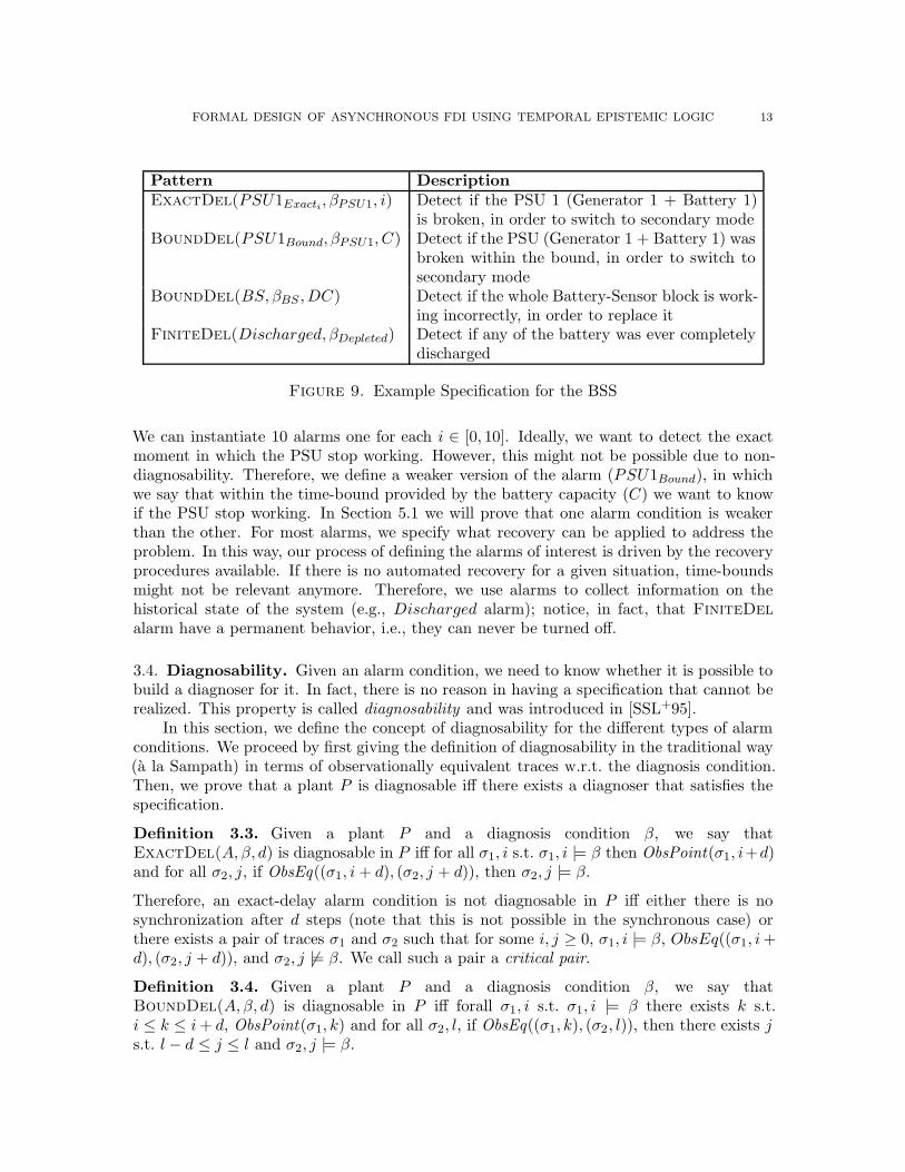
Figure 9 contains a simple specification for our running example. There are two typesof PSU (Power Supply Unit) alarms (that can be similarly defined for PSU 2). The first onedefines multiple alarms, each having a different delay i. Let us assume that each batteryhas a capacity C of 10, and that this provides us with a delay of at most 10 time-units.
FORMAL DESIGN OF ASYNCHRONOUS FDI USING TEMPORAL EPISTEMIC LOGIC 13
Pattern DescriptionExactDel(PSU1Exacti, βPSU1, i) Detect if the PSU 1 (Generator 1 + Battery 1)
is broken, in order to switch to secondary modeBoundDel(PSU1Bound, βPSU1, C) Detect if the PSU (Generator 1 + Battery 1) was
broken within the bound, in order to switch tosecondary mode
BoundDel(BS, βBS ,DC) Detect if the whole Battery-Sensor block is work-ing incorrectly, in order to replace it
FiniteDel(Discharged, βDepleted) Detect if any of the battery was ever completelydischarged
Figure 9. Example Specification for the BSS
We can instantiate 10 alarms one for each i ∈ [0, 10]. Ideally, we want to detect the exactmoment in which the PSU stop working. However, this might not be possible due to non-diagnosability. Therefore, we define a weaker version of the alarm (PSU1Bound), in whichwe say that within the time-bound provided by the battery capacity (C) we want to knowif the PSU stop working. In Section 5.1 we will prove that one alarm condition is weakerthan the other. For most alarms, we specify what recovery can be applied to address theproblem. In this way, our process of defining the alarms of interest is driven by the recoveryprocedures available. If there is no automated recovery for a given situation, time-boundsmight not be relevant anymore. Therefore, we use alarms to collect information on thehistorical state of the system (e.g., Discharged alarm); notice, in fact, that FiniteDelalarm have a permanent behavior, i.e., they can never be turned off.
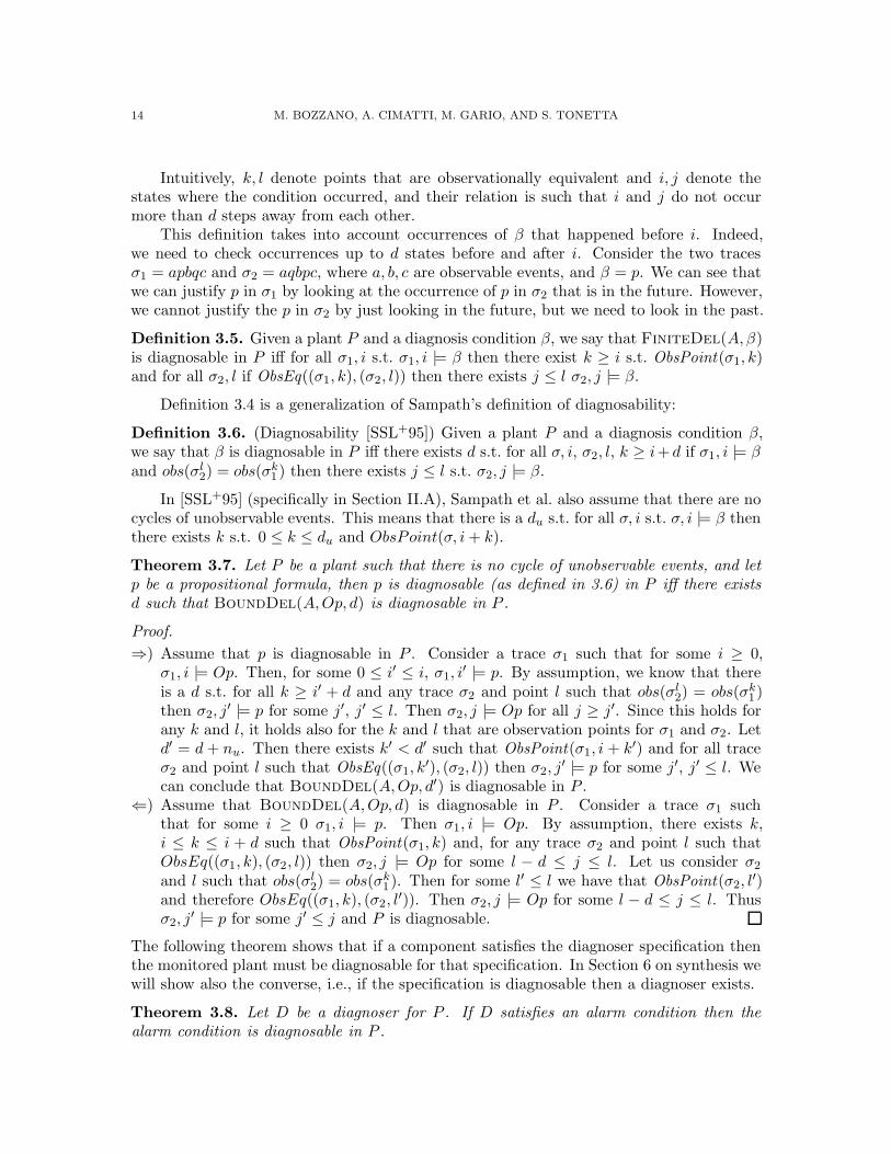
3.4. Diagnosability. Given an alarm condition, we need to know whether it is possible tobuild a diagnoser for it. In fact, there is no reason in having a specification that cannot berealized. This property is called diagnosability and was introduced in [SSL+95].
In this section, we define the concept of diagnosability for the different types of alarmconditions. We proceed by first giving the definition of diagnosability in the traditional way(a la Sampath) in terms of observationally equivalent traces w.r.t. the diagnosis condition.Then, we prove that a plant P is diagnosable iff there exists a diagnoser that satisfies thespecification.
Definition 3.3. Given a plant P and a diagnosis condition β, we say thatExactDel(A, β, d) is diagnosable in P iff for all σ1, i s.t. σ1, i |= β then ObsPoint(σ1, i+d)and for all σ2, j, if ObsEq((σ1, i+ d), (σ2, j + d)), then σ2, j |= β.
Therefore, an exact-delay alarm condition is not diagnosable in P iff either there is nosynchronization after d steps (note that this is not possible in the synchronous case) orthere exists a pair of traces σ1 and σ2 such that for some i, j ≥ 0, σ1, i |= β, ObsEq((σ1, i+d), (σ2, j + d)), and σ2, j 6|= β. We call such a pair a critical pair.
Definition 3.4. Given a plant P and a diagnosis condition β, we say thatBoundDel(A, β, d) is diagnosable in P iff forall σ1, i s.t. σ1, i |= β there exists k s.t.i ≤ k ≤ i+ d, ObsPoint(σ1, k) and for all σ2, l, if ObsEq((σ1, k), (σ2, l)), then there exists js.t. l − d ≤ j ≤ l and σ2, j |= β.
14 M. BOZZANO, A. CIMATTI, M. GARIO, AND S. TONETTA
Intuitively, k, l denote points that are observationally equivalent and i, j denote thestates where the condition occurred, and their relation is such that i and j do not occurmore than d steps away from each other.
This definition takes into account occurrences of β that happened before i. Indeed,we need to check occurrences up to d states before and after i. Consider the two tracesσ1 = apbqc and σ2 = aqbpc, where a, b, c are observable events, and β = p. We can see thatwe can justify p in σ1 by looking at the occurrence of p in σ2 that is in the future. However,we cannot justify the p in σ2 by just looking in the future, but we need to look in the past.
Definition 3.5. Given a plant P and a diagnosis condition β, we say that FiniteDel(A, β)is diagnosable in P iff for all σ1, i s.t. σ1, i |= β then there exist k ≥ i s.t. ObsPoint(σ1, k)and for all σ2, l if ObsEq((σ1, k), (σ2, l)) then there exists j ≤ l σ2, j |= β.
Definition 3.4 is a generalization of Sampath’s definition of diagnosability:
Definition 3.6. (Diagnosability [SSL+95]) Given a plant P and a diagnosis condition β,we say that β is diagnosable in P iff there exists d s.t. for all σ, i, σ2, l, k ≥ i+ d if σ1, i |= βand obs(σl2) = obs(σk1 ) then there exists j ≤ l s.t. σ2, j |= β.
In [SSL+95] (specifically in Section II.A), Sampath et al. also assume that there are nocycles of unobservable events. This means that there is a du s.t. for all σ, i s.t. σ, i |= β thenthere exists k s.t. 0 ≤ k ≤ du and ObsPoint(σ, i+ k).
Theorem 3.7. Let P be a plant such that there is no cycle of unobservable events, and letp be a propositional formula, then p is diagnosable (as defined in 3.6) in P iff there existsd such that BoundDel(A,Op, d) is diagnosable in P .
Proof.
⇒) Assume that p is diagnosable in P . Consider a trace σ1 such that for some i ≥ 0,σ1, i |= Op. Then, for some 0 ≤ i′ ≤ i, σ1, i
′ |= p. By assumption, we know that thereis a d s.t. for all k ≥ i′ + d and any trace σ2 and point l such that obs(σl2) = obs(σk1 )then σ2, j
′ |= p for some j′, j′ ≤ l. Then σ2, j |= Op for all j ≥ j′. Since this holds forany k and l, it holds also for the k and l that are observation points for σ1 and σ2. Letd′ = d+ nu. Then there exists k′ < d′ such that ObsPoint(σ1, i + k′) and for all traceσ2 and point l such that ObsEq((σ1, k
′), (σ2, l)) then σ2, j′ |= p for some j′, j′ ≤ l. We
can conclude that BoundDel(A,Op, d′) is diagnosable in P .⇐) Assume that BoundDel(A,Op, d) is diagnosable in P . Consider a trace σ1 such
that for some i ≥ 0 σ1, i |= p. Then σ1, i |= Op. By assumption, there exists k,i ≤ k ≤ i + d such that ObsPoint(σ1, k) and, for any trace σ2 and point l such thatObsEq((σ1, k), (σ2, l)) then σ2, j |= Op for some l − d ≤ j ≤ l. Let us consider σ2and l such that obs(σl2) = obs(σk1 ). Then for some l′ ≤ l we have that ObsPoint(σ2, l
′)and therefore ObsEq((σ1, k), (σ2, l
′)). Then σ2, j |= Op for some l − d ≤ j ≤ l. Thusσ2, j
′ |= p for some j′ ≤ j and P is diagnosable.
The following theorem shows that if a component satisfies the diagnoser specification thenthe monitored plant must be diagnosable for that specification. In Section 6 on synthesis wewill show also the converse, i.e., if the specification is diagnosable then a diagnoser exists.
Theorem 3.8. Let D be a diagnoser for P . If D satisfies an alarm condition then thealarm condition is diagnosable in P .
FORMAL DESIGN OF ASYNCHRONOUS FDI USING TEMPORAL EPISTEMIC LOGIC 15
Proof. By contradiction, suppose ExactDel(A, β, d) is not diagnosable in P . Then eitherthere exists a trace σ1 with σ1, i |= β for some i such that ObsPoint(σ1, j) is false for allj ≥ i or there exists a critical pair. In the first case, A is not triggered and the diagnoseris not complete. Suppose there exists a critical pair of traces σ1 and σ2, i.e., for somei, j ≥ 0 σ1, i |= β, ObsPoint(σ1, i+ d), ObsEq((σ1, i+ d), (σ2, j + d)), and σ2, j 6|= β. Since
D is deterministic, D(σ1) and D(σ2) have a common prefix compatible with obs(σi+d1 ) =
obs(σj+d2 ). If the diagnoser is complete then A is triggered in D(σ1)⊗ σ1 at position i+ d,
and so also in D(σ2) ⊗ σ2 at position j + d, but in this way the diagnoser is not correct,which is a contradiction. If the diagnoser is correct, then A is not triggered in D(σ2)⊗σ2 atposition j + d, but so neither in D(σ1)⊗ σ1 at position i+ d, but in this way the diagnoseris not complete, which is a contradiction.
Similarly, for FiniteDel(A, β) and BoundDel(A, β, d).
The definition above of diagnosability might be stronger than necessary, since diagnosabilityis defined as a global property of the plant. Imagine the situation in which there is a criticalpair and after removing this critical pair from the possible executions of the system, oursystem becomes diagnosable. This suggests that the system was “almost” diagnosable, andan ideal diagnoser would be able to perform a correct diagnosis in all the cases exceptone (i.e., the one represented by the critical pair). To capture this idea, we redefine theproblem of diagnosability from a global property expressed on the plant, to a local propertyexpressed on points of single traces.
Definition 3.9. Given a plant P , a diagnosis condition β and a trace σ1 such that forsome i ≥ 0 σ1, i |= β, we say that ExactDel(A, β, d) is trace diagnosable in 〈σ1, i〉 iffObsPoint(σ1, i+d) and for any trace σ2, for all j ≥ 0 such that ObsEq((σ1, i+d), (σ2, j+d)),σ2, j |= β.
Definition 3.10. Given a plant P , a diagnosis condition β, and a trace σ1 such that forsome i ≥ 0 σ1, i |= β, we say that BoundDel(A, β, d) is trace diagnosable in 〈σ1, i〉 iff thereexists k s.t. i ≤ k ≤ i+ d, ObsPoint(σ1, k), and for any σ2, l if ObsEq((σ1, k), (σ2, l)), thenthere exists j s.t. l − d ≤ k ≤ l and σ2, j |= β.
Definition 3.11. Given a plant P , a diagnosis condition β, and a trace σ1 such that forsome i ≥ 0, σ1, i |= β, we say that FiniteDel(A, β) is trace diagnosable in 〈σ1, i〉 iff thereexists k ≥ i s.t. ObsPoint(σ1, k) and for all σ2, l if ObsEq((σ1, k), (σ2, l)), then there existsj ≤ l and σ2, j |= β.
A specification that is trace diagnosable in a plant along all points of all traces isdiagnosable in the classical sense, and we say it is system diagnosable. The concept of tracediagnosability does not impose any specific behavior to the diagnoser. However, it is animportant concept that allows us to better characterize and understand the specificationand the system.
3.5. Maximality. As shown in Figure 8, bounded- and finite-delay alarms are correct ifthey are raised within the valid bound. However, there are several possible variations ofthe same alarm in which the alarm is active in different instants or for different periods.We address this problem by introducing the concept of maximality. Intuitively, a maximaldiagnoser is required to raise the alarms as soon as possible and as long as possible (withoutviolating the correctness condition).

16 M. BOZZANO, A. CIMATTI, M. GARIO, AND S. TONETTA
Definition 3.12. D is a maximal diagnoser for an alarm condition with alarm A in P iff forevery trace σP of P , D(σP ) contains the maximum number of observable points i such thatD(σP ), i |= A; that is, if D(σP ), i 6|= A, then there does not exist another correct diagnoserD′ of P such that D′(σP ), i |= A.
4. Formal Specification
In this section, we present the Alarm Specification Language with Epistemic operators(ASLK). This language allows designers to define requirements on the FDI alarms includingaspects such as delays, diagnosability and maximality.
Diagnosis conditions and alarm conditions are formalized using LTL with past operators.The definitions of trace diagnosability and maximality, however, cannot be captured byusing a formalization based on LTL. To capture these two concepts, we rely on temporalepistemic logic. The intuition is that this logic enables us to reason on set of observationallyequivalent traces instead that on single traces (like in LTL). We show how this logic canbe used to specify diagnosability, define requirements for non-diagnosable cases and expressthe concept of maximality.
4.1. Diagnosis and Alarm Conditions as LTL Properties. Let P be a set of proposi-tions representing either faults, events or elementary conditions for the diagnosis. The setDP of diagnosis conditions over P is any formula β built with the following rule:
β ::= p | β ∧ β | ¬β | Oβ | Y β
with p ∈ P.We provide the LTL characterization of the Alarm Specification Language (ASL) in
Figure 10. On the left column we provide the name of the alarm condition (as defined inthe previous section), and on the right column we provide the associated LTL formalizationencoding the concepts of correctness and completeness. Correctness, the first conjunct,intuitively says that whenever the diagnoser raises an alarm, then the fault must haveoccurred. Completeness, the second conjunct, intuitively encodes that whenever the faultoccurs, the alarm will be raised. In the following, for simplicity, we abuse notation andindicate with ϕ both the alarm condition and the associated LTL; for an alarm conditionϕ, we denote by Aϕ the associated alarm variable A, and with τ(ϕ) the following formulas:
τ(ϕ) = Y dβ for ϕ = ExactDel(A, β, d);τ(ϕ) = O≤dβ for ϕ = BoundDel(A, β, d);τ(ϕ) = Oβ for ϕ = FiniteDel(A, β).
When clear from the context, we use just A and τ instead of Aϕ and τ(ϕ), respectively.
Alarm Condition LTL Formulation
ExactDel(A, β, d) G(xAy→ Y dβ) ∧ G(β → Xd
xAy)
BoundDel(A, β, d) G(xAy→ O≤dβ) ∧ G(β → F≤d
xAy)
FiniteDel(A, β) G(xAy→ Oβ) ∧ G(β → F
xAy)
Figure 10. Alarm conditions as LTL (ASL): Correctness and Completeness
FORMAL DESIGN OF ASYNCHRONOUS FDI USING TEMPORAL EPISTEMIC LOGIC 17
Alarm Condition Diagnosability Maximality
ExactDel(A, β, d) G(β → XdxKY dβ
y) G(
xKY dβ
y→
xAy)
BoundDel(A, β, d) G(β → F≤dxKO≤dβ
y) G(
xKO≤dβ
y→
xAy)
FiniteDel(A, β) G(β → FxKOβ
y) G(
xKOβ
y→
xAy)
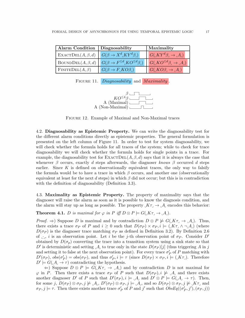
Figure 11. Diagnosability and Maximality .
βKO≤4β
A (Maximal)A (Non-Maximal)
Figure 12. Example of Maximal and Non-Maximal traces
4.2. Diagnosability as Epistemic Property. We can write the diagnosability test forthe different alarm conditions directly as epistemic properties. The general formulation ispresented on the left column of Figure 11. In order to test for system diagnosability, wewill check whether the formula holds for all traces of the system; while to check for tracediagnosability we will check whether the formula holds for single points in a trace. Forexample, the diagnosability test for ExactDel(A, β, d) says that it is always the case thatwhenever β occurs, exactly d steps afterwards, the diagnoser knows β occurred d stepsearlier. Since K is defined on observationally equivalent traces, the only way to falsifythe formula would be to have a trace in which β occurs, and another one (observationallyequivalent at least for the next d steps) in which β did not occur; but this is in contradictionwith the definition of diagnosability (Definition 3.3).
4.3. Maximality as Epistemic Property. The property of maximality says that thediagnoser will raise the alarm as soon as it is possible to know the diagnosis condition, andthe alarm will stay up as long as possible. The property
xKτ
y→
xAyencodes this behavior:
Theorem 4.1. D is maximal for ϕ in P iff D ⊗ P |= G(xKτ
y→
xAy).
Proof. ⇒) Suppose D is maximal and by contradiction D ⊗ P 6|= G(xKτ
y→
xAy). Thus,
there exists a trace σP of P and i ≥ 0 such that D(σP ) × σP , i |= (xKτ
y∧ ¬
xAy) (where
D(σP ) is the diagnoser trace matching σP as defined in Definition 3.2). By Definition 2.6of
x·y, i is an observation point. Let i be the j-th observation point of σP . Consider D′
obtained by D(σp) converting the trace into a transition system using a sink state so thatD′ is deterministic and setting
xAyto true only in the state D(σP )[j] (thus triggering A in j
and setting it to false at the next observation point). For every trace σ′P of P matching withD′(σP ), obs(σ
′P ) = obs(σP ), and thus σ′P , i |= τ (since D(σP ) × σP , i |= (
xKτ
y). Therefore
D′ |= G(xAy→ τ) contradicting the hypothesis.
⇐) Suppose D ⊗ P |= G(xKτ
y→
xAy) and by contradiction D is not maximal for
ϕ in P . Then there exists a trace σP of P such that D(σP ), i 6|= xAyand there exists
another diagnoser D′ of P such that D′(σP ), i |= xAyand D′ ⊗ P |= G(
xAy→ τ). Then,
for some j, D(σP )⊗ σP , j 6|= xAy, D′(σP )⊗ σP , j |= x
Ay, and so D(σP ) ⊗ σP , j 6|= x
Kτyand
σP , j |= τ . Then there exists another trace σ′P of P and j′ such that ObsEq((σ′P , j′), (σP , j))

18 M. BOZZANO, A. CIMATTI, M. GARIO, AND S. TONETTA
and σ′P , j′ 6|= τ . Since D′ is deterministic, D′(σ′P ) and D′(σP ) are equal up to position i,
and so D′ ⊗ P 6|= G(xAy→ τ) contradicting the hypothesis.
Whenever the diagnoser knows that τ is satisfied, it will raise the alarm. An example ofmaximal and non-maximal alarm is given in Figure 12. Note that according to our definition,the set of maximal alarms is a subset of the non-maximal ones.
A property related to Maximality is the capability of the diagnoser to justify the raisingof the alarm. This property is guaranteed by construction by any correct diagnoser, as shownin the following theorem.
Theorem 4.2. Given a diagnoser D and a plant P , for each alarm A of D, with temporalcondition τ , if D is correct for A it holds that:
D ⊗ P |= G(xAy→
xKτ
y)
Thus, whenever the diagnoser raises an alarm, it knows that the diagnosis condition hasoccurred.
Proof. We assume by contradiction that the G(xAy→
xKτ
y) is not satisfied. Therefore,
there exist σ and i such that D(σ)⊗σ, i |=xAy∧¬
xKτ
y(where D(σP ) is the diagnoser trace
matching σP as defined in Definition 3.2), which is equivalent toxAy∧¬Kτ (by Definition 2.6
ofx·y). Thus, σ, i |= τ by correctness of D. In order for the ¬Kτ to hold, we need another
trace σ′ and j s.t. ObsEq((σ, i), (σ′, j)) and σ′, j |= ¬τ . By definition, the diagnoser isdeterministic, thus we know that for σ, σ′ at points i, j we will have the same value of A.Therefore, D(σ′)⊗σ′, j |=
xAy∧¬τ so that D is not correct, thus reaching a contradiction.
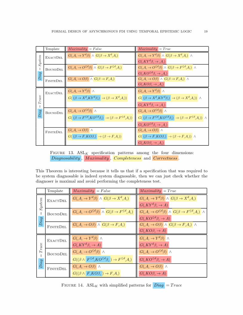
4.4. ASLK Specifications. The formalization of ASLK (Figure 13) is obtained by extend-ing ASL (Figure 10) with the concepts of maximality and diagnosability, defined as epistemicproperties. When maximality is required we add a third conjunct following Theorem 4.1.When Diag = Trace instead, we precondition the completeness to the trace diagnosability(as defined in Figure 11); this means that the diagnoser will raise an alarm whenever thediagnosis condition is satisfied and the diagnoser is able to know it.
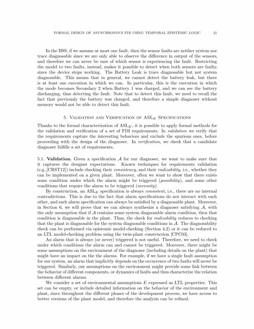
Several simplifications are possible. For example, in the case Diag = Trace, we do notneed to verify the completeness due to the following result:
Theorem 4.3. Given a diagnoser D for a plant P and a trace diagnosable alarm conditionϕ, if D is maximal for ϕ, then D is complete.
Proof. (ExactDel) For all σ, i if σ, i |= (β → XdxKY dβ
y), then by using the maximality
assumption, we know that σ, i |= (β → XdxAy); thus, σ, i |= (β → Xd
xKY dβ
y) → (β →
XdxAy). Similarly we can prove BoundDel and FiniteDel.
As a corollary of Theorem 4.3, the same can be applied also for system diagnosable alarmconditions if P is diagnosable, since system diagnosability implies trace diagnosability:
Theorem 4.4. Given an alarm condition for the system diagnosable case, and a diagnoserD for a plant P , if D is maximal for ϕ and ϕ is diagnosable in P then D is complete.
Proof. The theorem follows directly from Theorem 4.3 and the fact that if D is completefor a trace diagnosable alarm condition that is system diagnosable, then D is also completefor the corresponding system diagnosable alarm condition.
FORMAL DESIGN OF ASYNCHRONOUS FDI USING TEMPORAL EPISTEMIC LOGIC 19
Template Maximality = False Maximality = True
Diag
=System ExactDel
G(xAy→ Y dβ) ∧ G(β → Xd
xAy) G(
xAy→ Y dβ) ∧ G(β → Xd
xAy) ∧
G(xKY dβ
y→
xAy)
BoundDelG(
xAy→ O≤dβ) ∧ G(β → F≤d
xAy) G(
xAy→ O≤dβ) ∧ G(β → F≤d
xAy) ∧
G(xKO≤dβ
y→
xAy)
FiniteDelG(
xAy→ Oβ) ∧ G(β → F
xAy) G(
xAy→ Oβ) ∧ G(β → F
xAy) ∧
G(xKOβ
y→
xAy)
Diag
=Trace
ExactDelG(
xAy→ Y dβ) ∧ G(
xAy→ Y dβ) ∧
G( (β → XdxKY dβ
y) → (β → Xd
xAy)) G( (β → Xd
xKY dβ
y) → (β → Xd
xAy)) ∧
G(xKY dβ
y→
xAy)
BoundDelG(
xAy→ O≤dβ) ∧ G(
xAy→ O≤dβ) ∧
G( (β → F≤dxKO≤dβ
y) → (β → F≤d
xAy)) G( (β → F≤d
xKO≤dβ
y) → (β → F≤d
xAy)) ∧
G(xKO≤dβ
y→
xAy)
FiniteDelG(
xAy→ Oβ) ∧ G(
xAy→ Oβ) ∧
G( (β → FxKOβ
y) → (β → F
xAy)) G( (β → F
xKOβ
y) → (β → F
xAy)) ∧
G(xKOβ
y→
xAy)
Figure 13. ASLK specification patterns among the four dimensions:
Diagnosability , Maximality , Completeness and Correctness .
This Theorem is interesting because it tells us that if a specification that was required tobe system diagnosable is indeed system diagnosable, then we can just check whether thediagnoser is maximal and avoid performing the completeness test.
Template Maximality = False Maximality = True
Diag
=System ExactDel
G(xAy→ Y dβ) ∧ G(β → Xd
xAy) G(
xAy→ Y dβ) ∧ G(β → Xd
xAy)
G(xKY dβ
y→ A)
BoundDelG(
xAy→ O≤dβ) ∧ G(β → F≤d
xAy) G(
xAy→ O≤dβ) ∧ G(β → F≤d
xAy) ∧
G(xKO≤dβ
y→ A)
FiniteDelG(
xAy→ Oβ) ∧ G(β → F
xAy) G(
xAy→ Oβ) ∧ G(β → F
xAy) ∧
G(xKOβ
y→ A)
Diag
=Trace
ExactDelG(
xAy→ Y dβ) ∧ G(
xAy→ Y dβ) ∧
G(xKY dβ
y→ A) G(
xKY dβ
y→ A)
BoundDelG(
xAy→ O≤dβ) ∧ G(
xAy→ O≤dβ) ∧
G((β ∧ F≤dxKO≤dβ
y)→ F≤d
xAy) G(
xKO≤dβ
y→ A)
FiniteDelG(
xAy→ Oβ) ∧ G(
xAy→ Oβ) ∧
G((β ∧ FxKOβ
y)→ F
xAy) G(
xKOβ
y→ A)
Figure 14. ASLK with simplified patterns for Diag = Trace

20 M. BOZZANO, A. CIMATTI, M. GARIO, AND S. TONETTA
Theorem 4.5. For all trace diagnosable and non-maximal ExactDel specifications, com-pleteness can be replaced by maximality. Formally, for all σ, σ |= G((β → Xd
xKY dβ
y) →
(β → XdxAy)) iff σ |= G(
xKY dβ
y→
xAy)
Proof.
σ, i |=((β → XdxKY dβ
y)→ (β → Xd
xAy)) iff
σ, i |=((β ∧XdxKY dβ
y)→ Xd
xAy) iff
σ, i+ d |=((Y dβ ∧xKY dβ
y)→
xAy) iff
σ, i+ d |=((xY dβ ∧KY dβ
y)→
xAy) iff
σ, i+ d |=(xKY dβ
y→
xAy)
Therefore, we can conclude that for all i, σ, i |= ((β → XdxKY dβ
y) → (β → Xd
xAy)) iff for
all j ≥ d, σ, j |= (xKY dβ
y→
xAy). We conclude noting that for j < d, Y dβ is false and
therefore σ, j |= (xKY dβ
y→
xAy).
After applying the simplifications specified in Theorem 4.3 and Theorem 4.5 and theequivalence
xφy→
xψy≡
xφy→ ψ, we obtain the table in Figure 14, where the patterns in
the lower half (Diag = Trace) have been simplified.An ASLK specification is built by instantiating the patterns defined in Figure 13. For
example, we would write ExactDelK(A, β, d, T race, T rue) for an exact-delay alarm Afor β with delay d, that satisfies the trace diagnosability property and is maximal. Anintroductory example on the usage of ASLK for the specification of a diagnoser is providedin [BCGT13]. Figure 15 shows how we extend the specification for the BSS by introducingrequirements on the diagnosability and maximality of alarms. In particular, all the alarmsthat we defined are not system diagnosable. Therefore, we need to weaken the requirementsand make them trace-diagnosable. The patterns are then converted into temporal epistemicformulae as shown in Figure 16.
ExactDelK(PSU1Exacti , βPSU1, i, T race, T rue)BoundDelK(PSU1Bound, βPSU1, C, T race, T rue)BoundDelK(BS, βBS ,DC, Trace, T rue)FiniteDelK(Discharged, βDepleted, T race, False)FiniteDelK(B1Leak, βBattery1, System, True)
Figure 15. ASLK Specification for the BSS
Alarm Formula
PSU1Exacti G(xPSU1Exactiy → Y iβPSU1) ∧ G(
xKY iβPSU1y → x
PSU1Exactiy)
PSU1Bound G(xPSU1Boundy → O≤CβPSU1) ∧ G(
xKO≤CβPSU1y → x
PSU1Boundy)
BS G(xBS
y→ O≤DCβBS) ∧ G(
xKO≤DCβBSy → x
BSy)
Discharged G(xDischarged
y→ OβDeplated) ∧ G((βDeplated ∧ F
xKOβDeplatedy )→ F
xDischarged
y)
B1Leak G(xB1Leak
y→ OβBattery1) ∧ G(βBattery1 → F
xB1Leak
y) ∧ G(
xKOβBattery1y → x
B1Leaky)
Figure 16. KL1 translation of ASLK patterns for the BSS
FORMAL DESIGN OF ASYNCHRONOUS FDI USING TEMPORAL EPISTEMIC LOGIC 21
In the BSS, if we assume at most one fault, then the sensor faults are neither system nortrace diagnosable since we are only able to observe the difference in output of the sensors,and therefore we can never be sure of which sensor is experiencing the fault. Restrictingthe model to two faults, instead, makes it possible to detect when both sensors are faulty,since the device stops working. The Battery Leak is trace diagnosable but not systemdiagnosable. This means that in general, we cannot detect the battery leak, but thereis at least one execution in which we can. In particular, this is the execution in whichthe mode becomes Secondary 2 when Battery 1 was charged, and we can see the batterydischarging, thus detecting the fault. Note that to detect this fault, we need to recall thefact that previously the battery was charged, and therefore a simple diagnoser withoutmemory would not be able to detect this fault.
5. Validation and Verification of ASLK Specifications
Thanks to the formal characterization of ASLK , it is possible to apply formal methods forthe validation and verification of a set of FDI requirements. In validation we verify thatthe requirements capture the interesting behaviors and exclude the spurious ones, beforeproceeding with the design of the diagnoser. In verification, we check that a candidatediagnoser fulfills a set of requirements.
5.1. Validation. Given a specification A for our diagnoser, we want to make sure thatit captures the designer expectations. Known techniques for requirements validation(e.g.,[CRST12]) include checking their consistency, and their realizability, i.e., whether theycan be implemented on a given plant. Moreover, often we want to show that there existssome condition under which the alarm might be triggered (possibility), and some otherconditions that require the alarm to be triggered (necessity).
By construction, an ASLK specification is always consistent, i.e., there are no internalcontradictions. This is due to the fact that alarm specifications do not interact with eachother, and each alarm specification can always be satisfied by a diagnosable plant. Moreover,in Section 6, we will prove that we can always synthesize a diagnoser satisfying A, withthe only assumption that if A contains some system diagnosable alarm condition, then thatcondition is diagnosable in the plant. Thus, the check for realizability reduces to checkingthat the plant is diagnosable for the system diagnosable conditions in A. The diagnosabilitycheck can be performed via epistemic model-checking (Section 4.2) or it can be reduced toan LTL model-checking problem using the twin-plant construction [CPC03].
An alarm that is always (or never) triggered is not useful. Therefore, we need to checkunder which conditions the alarm can and cannot be triggered. Moreover, there might besome assumptions on the environment of the diagnoser (including details on the plant) thatmight have an impact on the the alarms. For example, if we have a single fault assumptionfor our system, an alarm that implicitly depends on the occurrence of two faults will never betriggered. Similarly, our assumptions on the environment might provide some link betweenthe behavior of different components, or dynamics of faults and thus characterize the relationbetween different alarms.
We consider a set of environmental assumptions E expressed as LTL properties. Thisset can be empty, or include detailed information on the behavior of the environment andplant, since throughout the different phases of the development process, we have access tobetter versions of the plant model, and therefore the analysis can be refined.

22 M. BOZZANO, A. CIMATTI, M. GARIO, AND S. TONETTA
When checking possibility we want that the alarms can be eventually activated, butalso that they are not always active. This means that for a given alarm condition ϕ ∈ A,we are interested in verifying that there is a trace σ ∈ E and a trace σ′ ∈ E s.t. σ |= F
xAϕy
and σ′ |= F¬xAϕy. This can be done by checking the unsatisfiability of (E ∧ ϕ) → G¬
xAϕy
and (E ∧ ϕ)→ GxAϕy.
Checking necessity provides us a way to understand whether there is some correlationbetween alarms. This, in turns, makes it possible to simplify the model, or to guaranteesome redundancy requirement. To check whether Aϕ′ is a more general alarm than Aϕ
(subsumption) we check whether (E ∧ ϕ ∧ ϕ′) → G(xAϕy → x
Aϕ′y) is valid. An example of
subsumption of alarms is given by the definition of maximality: any non-maximal alarmsubsumes its corresponding maximal version. Finally, we can verify that two alarms aremutually exclusive by checking the validity of (E ∧ ϕ ∧ ϕ′)→ G¬(
xAϕy ∧ x
Aϕ′y).
To clarify the concepts presented in this section, we apply a necessity check on ourrunning example. In the Battery-Sensor, we have two alarms specified on PSU1 (Figure 15):PSU1Exacti and PSU1Bound. Let’s take i = C = 2, thus obtaining:
- ExactDelK(PSU1Exact2 , βPSU1, 2, T race, T rue)- BoundDelK(PSU1Bound, βPSU1, 2, T race, T rue)
we want to show that PSU1Exacti is more specific than (is subsumed by) PSU1Bound. Thismeans that for any plant and diagnoser, the following holds:
D ⊗ P |= (ϕPSU1Exact2∧ ϕ′
PSU1Bound)→ G(
xPSU1Exact2y → x
PSU1Boundy)
By renaming with PE = PSU1Exact2 and PB = PSUBound (for brevity) and expandingthe definitions of ϕPSU1Exact2
∧ ϕ′PSU1Bound
we have that
D ⊗ P |= (G(xPE
y→ Y 2β) ∧G(
xKY 2β
y→
xPE
y) ∧
G(xPB
y→ O≤2β) ∧G(
xKO≤2β
y→
xPB
y))
→ G(xPE
y→
xPB
y)
We can apply Theorem 4.2, and therefore write:
D ⊗ P |= (G(xPE
y→ Y 2β) ∧G(
xKY 2β
y→
xPE
y) ∧
G(xPB
y→ O≤2β) ∧G(
xKO≤2β
y→
xPB
y) ∧
G(xPE
y→
xKY 2β
y) ∧G(
xPB
y→
xKO≤2β
y))
→ G(xPE
y→
xPB
y)
To prove that the above formula is valid (and therefore it is satisfied by any plant anddiagnoser), we prove that its negation is unsatisfiable:
(G(xPE
y→ Y 2β) ∧G(
xKY 2β
y→
xPE
y) ∧
G(xPB
y→ O≤2β) ∧G(
xKO≤2β
y→
xPB
y) ∧
G(xPE
y→
xKY 2β
y) ∧G(
xPB
y→
xKO≤2β
y))
∧¬G(xPE
y→
xPB
y)
The first part of this formula is composed by conjuncts in the form Gψ. This means that acounter examples is a trace for which each state satisfies ψ. Moreover, we need one of thesestates to satisfy (PE ∧ ¬
xPB
y). Therefore, to prove the unsatisfiable of the above formula,

FORMAL DESIGN OF ASYNCHRONOUS FDI USING TEMPORAL EPISTEMIC LOGIC 23
we can just prove that no state exists that satisfies:
(xPE
y→ Y 2β) ∧ (
xKY 2β
y→
xPE
y) ∧
(xPB
y→ O≤2β) ∧ (
xKO≤2β
y→
xPB
y) ∧
(xPE
y→
xKY 2β
y) ∧ (
xPB
y→
xKO≤2β
y))
∧xPE
y∧ ¬
xPB
y
We show this by a contradiction since:
· · · ∧xPE
y∧ ¬
xPB
y
ObsPoint Def. · · · ∧x⊤y∧ PE ∧ ¬PB
Theorem 4.2 on PE · · · ∧x⊤y∧ PE ∧ ¬PB ∧KY Y β
Maximality of PB · · · ∧x⊤y∧ PE ∧ ¬PB ∧KY Y β ∧ ¬KO≤2β
†Def. of ¬K · · · ∧x⊤y∧ PE ∧ ¬PB ∧KY Y β ∧ ¬O≤2β
Def. of O≤n · · · ∧x⊤y∧ PE ∧ ¬PB ∧KY Y β ∧ ¬(β ∨ Y β ∨ Y Y β)
K Axiom (Kφ→ φ) · · · ∧x⊤y∧ PE ∧ ¬PB ∧ Y Y β ∧ ¬β ∧ ¬Y β ∧ ¬Y Y β
Thus reaching a contradiction between Y Y β and ¬Y Y β. In the step marked with † weneed to show that two observationally equivalent traces exists s.t. one satisfies O≤2β andthe other ¬O≤2β; therefore, we only need to show that one of the two (namely ¬O≤2β)does not exist.
5.2. Verification. The verification of a system w.r.t. a specification can be performed viamodel-checking techniques using the semantics of the alarm conditions:
Definition 5.1. Let D be a diagnoser for alarms A and plant P . We say that D satisfiesa set A of ASLK specifications iff for each ϕ in AP there exists an alarm Aϕ ∈ A andD ⊗ P |= ϕ.
To perform this verification steps, we need in general a model checker for KL1 with asyn-chronous/synchronous perfect recall such as MCK [GM04]. However, if the specificationfalls in the pure LTL fragment (ASL) we can verify it with an LTL model-checker such asnuXmv [CCD+14] thus benefiting from the efficiency of the tools in this area.
Moreover, a diagnoser is required to be deterministic. This is important, on one hand,for implementability, on the other hand, to ensure that the composition of the plant withthe diagnoser does not reduce the behaviors of the plant. In order to verify that a givendiagnoser D = 〈V,E, I,T 〉 is deterministic, we check the following conditions:
• I must be satisfiable,• I ∧ I[Vc/V ]→ V = Vc must be valid,• for all e ∈ E, ∀V ∃V ′.T (e) must be valid (note that this corresponds to the validity of thepre-image of ⊤),• for all e ∈ E, T (e) ∧ T (e)[Vc/V
′]→ V ′ = Vc must be valid.
Therefore, we can solve the problem with a finite set of satisfiability checks and pre-imagecomputations.
24 M. BOZZANO, A. CIMATTI, M. GARIO, AND S. TONETTA
6. Synthesis of a Diagnoser from an ASLK Specification
In this section, we discuss how to synthesize a diagnoser that satisfies a given specificationA. We considers the most expressive case of ASLK (maximal/trace diagnosable), whichalso satisfies all the other cases.
The idea is to generate an automaton that encodes the set of possible states in whichthe plant could be after each observations. The result is achieved by generating the power-set of the states of the plant, also called belief states, and defining a suitable transitionrelation among the elements of this set, only taking into account observable information.Each belief state of the automaton is then annotated with the alarms that are satisfied inall the states of the belief state. The resulting automaton is the Diagnoser.
The approach resembles the constructions by Sampath [SSL+96] and Schumann [Sch04],with the following main differences. First, we consider LTL Past expression as diagnosiscondition, and not only fault events as done in previous works. Second, instead of providinga set of possible diagnoses, we provide alarms. In order to raise the alarm, we need to becertain that the alarm condition is satisfied for all possible diagnoses. This gives raise to a3-valued alarm system: we know that the fault occurred; know that the fault did not occur;or we are uncertain. Moreover, the approach works for the asynchronous case. Althoughthe use of a power-set construction in the setting of temporal epistemic logic is not novel(e.g. [Dim09] for synchronous CTLK model-checking), the main contribution of this sectionis to show the formal properties of the diagnoser, and in particular that it satisfies thespecification. In a way, this algorithm is a strong indicator of a deep connection betweenthe topics of temporal epistemic logic reasoning and FDI design.
6.1. Synthesis algorithm. Given a partially observable plant P = 〈V P , EP , IP ,T P , EP0 〉,
let S be the set of states of P . The belief automaton is defined as B(P ) = 〈B,E, b0, R〉where B = 2S , E = EP
o , b0 ∈ B and R : (B×E)→ B. B represents the set of sets of states,also called belief states. Given a belief state b, we use b∗ to represent the set of states thatare reachable from b by only using events in EP \EP
o (non observable events), and call it theu-transitive closure. Formally, b∗ is the least set s.t. b ⊆ b∗ and if there exist e ∈ EP \ EP
o
and s′ ∈ b∗ such that 〈s′, s〉 ∈ T P (e) then s ∈ b∗. b0 is the initial belief state and containsthe states that satisfy the initial condition IP (i.e., b0 = {s | s |= IP }).
Given a belief state b and an observable event e ∈ EPo , we define the successor belief
state b′ as:R(b, e) = b′ = {s′ | ∃s ∈ b∗. 〈s, s′〉 |= TP (e)}
that is the set of states that are compatible with the observable event e in a state of theu-transitive closure of b. Intuitively, we first compute the u-transitive closure of b to accountfor all non-observable transitions, and then we consider all the different states that can bereached from b∗ with an occurrence of the event e.
The diagnoser is obtained by annotating each state of the belief automaton with thecorresponding alarms. We annotate with Aϕ all the states b that satisfy the temporalproperty τ(ϕ). As explained later on, any temporal τ(ϕ) can be handled by introducingsuitable propositional formulas. Therefore we consider the simplest case in which τ(ϕ) isa propositional formula and formally say that the annotation ab of the belief state b is theassignment to Aϕ such that ab(Aϕ) is true iff for all s ∈ b, s |= τ(ϕ). We perform thesame annotation for A¬ϕ. The diagnoser obtained by this algorithm induces three alarms,related to the knowledge of the diagnoser. In particular, the diagnoser can be sure that
FORMAL DESIGN OF ASYNCHRONOUS FDI USING TEMPORAL EPISTEMIC LOGIC 25
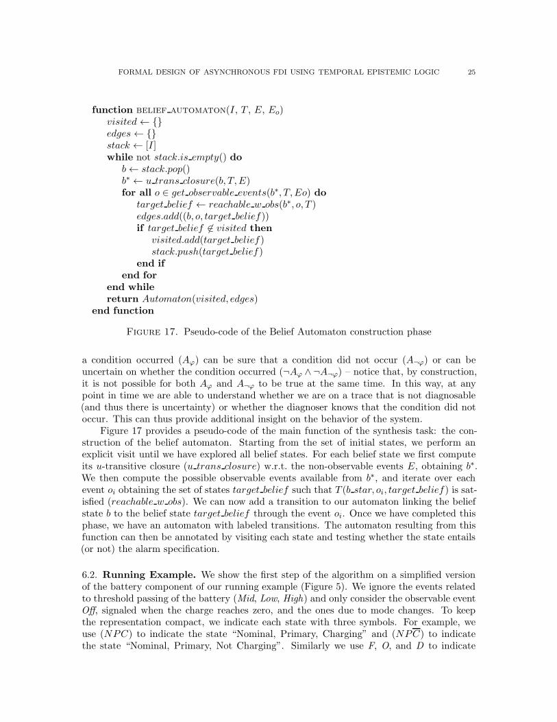
function belief automaton(I, T , E, Eo)visited← {}edges ← {}stack ← [I]while not stack.is empty() do
b← stack.pop()b∗ ← u trans closure(b, T,E)for all o ∈ get observable events(b∗, T,Eo) do
target belief ← reachable w obs(b∗, o, T )edges.add((b, o, target belief))if target belief 6∈ visited then
visited.add(target belief)stack.push(target belief)
end ifend for
end whilereturn Automaton(visited, edges)
end function
Figure 17. Pseudo-code of the Belief Automaton construction phase
a condition occurred (Aϕ) can be sure that a condition did not occur (A¬ϕ) or can beuncertain on whether the condition occurred (¬Aϕ ∧ ¬A¬ϕ) – notice that, by construction,it is not possible for both Aϕ and A¬ϕ to be true at the same time. In this way, at anypoint in time we are able to understand whether we are on a trace that is not diagnosable(and thus there is uncertainty) or whether the diagnoser knows that the condition did notoccur. This can thus provide additional insight on the behavior of the system.
Figure 17 provides a pseudo-code of the main function of the synthesis task: the con-struction of the belief automaton. Starting from the set of initial states, we perform anexplicit visit until we have explored all belief states. For each belief state we first computeits u-transitive closure (u trans closure) w.r.t. the non-observable events E, obtaining b∗.We then compute the possible observable events available from b∗, and iterate over eachevent oi obtaining the set of states target belief such that T (b star, oi, target belief) is sat-isfied (reachable w obs). We can now add a transition to our automaton linking the beliefstate b to the belief state target belief through the event oi. Once we have completed thisphase, we have an automaton with labeled transitions. The automaton resulting from thisfunction can then be annotated by visiting each state and testing whether the state entails(or not) the alarm specification.
6.2. Running Example. We show the first step of the algorithm on a simplified versionof the battery component of our running example (Figure 5). We ignore the events relatedto threshold passing of the battery (Mid, Low, High) and only consider the observable eventOff, signaled when the charge reaches zero, and the ones due to mode changes. To keepthe representation compact, we indicate each state with three symbols. For example, weuse (NPC) to indicate the state “Nominal, Primary, Charging” and (NPC) to indicatethe state “Nominal, Primary, Not Charging”. Similarly we use F, O, and D to indicate
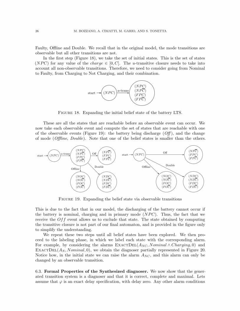
26 M. BOZZANO, A. CIMATTI, M. GARIO, AND S. TONETTA
Faulty, Offline and Double. We recall that in the original model, the mode transitions areobservable but all other transitions are not.
In the first step (Figure 18), we take the set of initial states. This is the set of states(NPC) for any value of the charge ∈ [0, C]. The u-transitive closure needs to take intoaccount all non-observable transitions. Therefore, we need to consider going from Nominalto Faulty, from Charging to Not Charging, and their combination.
(NPC)start
(NPC)(NPC)(FPC)(FPC)
u-trans
Figure 18. Expanding the initial belief state of the battery LTS.
These are all the states that are reachable before an observable event can occur. Wenow take each observable event and compute the set of states that are reachable with oneof the observable events (Figure 19): the battery being discharge (Off ), and the changeof mode (Offline, Double). Note that one of the belief states is smaller than the others.
(NPC)start
(NPC)(NPC)(FPC)(FPC)
(NOC)(NOC)(FOC)(FOC)
(NDC)(NDC)(FDC)(FDC)
(NPC)(FPC)(FPC)
u-trans
OfflineDouble
Off (NPC)start
(NOC)(NOC)(FOC)(FOC)
(NDC)(NDC)(FDC)(FDC)
(NPC)(FPC)(FPC)
OfflineDouble
Off
Figure 19. Expanding the belief state via observable transitions
This is due to the fact that in our model, the discharging of the battery cannot occur ifthe battery is nominal, charging and in primary mode (NPC). Thus, the fact that wereceive the Off event allows us to exclude that state. The state obtained by computingthe transitive closure is not part of our final automaton, and is provided in the figure onlyto simplify the understanding.
We repeat these two steps until all belief states have been explored. We then pro-ceed to the labeling phase, in which we label each state with the corresponding alarm.For example, by considering the alarms ExactDel(ANC , Nominal ∧ Charging, 0) andExactDel(AN , Nominal, 0), we obtain the diagnoser partially represented in Figure 20.Notice how, in the initial state we can raise the alarm ANC , and this alarm can only bechanged by an observable transition.
6.3. Formal Properties of the Synthesized diagnoser. We now show that the gener-ated transition system is a diagnoser and that it is correct, complete and maximal. Letsassume that ϕ is an exact delay specification, with delay zero. Any other alarm conditions
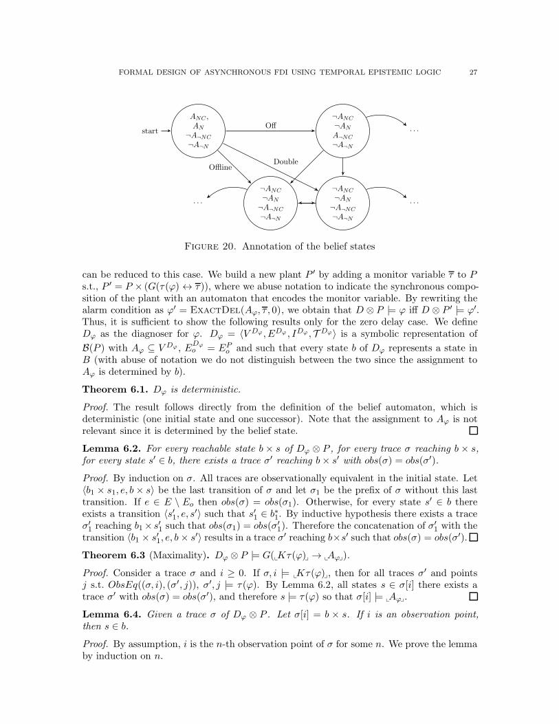
FORMAL DESIGN OF ASYNCHRONOUS FDI USING TEMPORAL EPISTEMIC LOGIC 27
ANC ,AN
¬A¬NC
¬A¬N
start
¬ANC
¬AN
¬A¬NC
¬A¬N
¬ANC
¬AN
¬A¬NC
¬A¬N
¬ANC
¬AN
A¬NC
¬A¬N
· · · · · ·
· · ·
OfflineDouble
Off
Figure 20. Annotation of the belief states
can be reduced to this case. We build a new plant P ′ by adding a monitor variable τ to Ps.t., P ′ = P × (G(τ(ϕ) ↔ τ)), where we abuse notation to indicate the synchronous compo-sition of the plant with an automaton that encodes the monitor variable. By rewriting thealarm condition as ϕ′ = ExactDel(Aϕ, τ , 0), we obtain that D ⊗ P |= ϕ iff D ⊗ P ′ |= ϕ′.Thus, it is sufficient to show the following results only for the zero delay case. We defineDϕ as the diagnoser for ϕ. Dϕ = 〈V Dϕ , EDϕ , IDϕ ,T Dϕ〉 is a symbolic representation of
B(P ) with Aϕ ⊆ V Dϕ , EDϕo = EP
o and such that every state b of Dϕ represents a state inB (with abuse of notation we do not distinguish between the two since the assignment toAϕ is determined by b).
Theorem 6.1. Dϕ is deterministic.
Proof. The result follows directly from the definition of the belief automaton, which isdeterministic (one initial state and one successor). Note that the assignment to Aϕ is notrelevant since it is determined by the belief state.
Lemma 6.2. For every reachable state b × s of Dϕ ⊗ P , for every trace σ reaching b × s,for every state s′ ∈ b, there exists a trace σ′ reaching b× s′ with obs(σ) = obs(σ′).
Proof. By induction on σ. All traces are observationally equivalent in the initial state. Let〈b1 × s1, e, b× s〉 be the last transition of σ and let σ1 be the prefix of σ without this lasttransition. If e ∈ E \ Eo then obs(σ) = obs(σ1). Otherwise, for every state s′ ∈ b thereexists a transition 〈s′1, e, s
′〉 such that s′1 ∈ b∗1. By inductive hypothesis there exists a trace
σ′1 reaching b1× s′1 such that obs(σ1) = obs(σ′1). Therefore the concatenation of σ′1 with the
transition 〈b1 × s′1, e, b× s
′〉 results in a trace σ′ reaching b×s′ such that obs(σ) = obs(σ′).
Theorem 6.3 (Maximality). Dϕ ⊗ P |= G(xKτ(ϕ)
y→
xAϕy).
Proof. Consider a trace σ and i ≥ 0. If σ, i |=xKτ(ϕ)
y, then for all traces σ′ and points
j s.t. ObsEq((σ, i), (σ′, j)), σ′, j |= τ(ϕ). By Lemma 6.2, all states s ∈ σ[i] there exists atrace σ′ with obs(σ) = obs(σ′), and therefore s |= τ(ϕ) so that σ[i] |=
xAϕy.
Lemma 6.4. Given a trace σ of Dϕ ⊗ P . Let σ[i] = b × s. If i is an observation point,then s ∈ b.
Proof. By assumption, i is the n-th observation point of σ for some n. We prove the lemmaby induction on n.
28 M. BOZZANO, A. CIMATTI, M. GARIO, AND S. TONETTA
Consider the case n = 1. If σ[0] = b0 × s0, by construction of Dϕ, s0 ∈ b0. Letσ[i − 1] = b′ × s′ and let e be the i-th (observable) event of σ. If i is the first observationpoint of σ, it means that b′ = b0 and s′ ∈ b∗0. Moreover, 〈s′, s〉 ∈ T (e) and therefore s ∈ b.
Consider the case n > 1. Let j be the n− 1 observation point, σ[j] = bj × sj, σ[i− 1] =b′ × s′ and let e be the i-th (observable) event of σ. Similarly to the previous case, b′ = bjand s′ ∈ b∗j . Moreover 〈s′, s〉 ∈ T (e) and therefore s ∈ b.
Theorem 6.5 (Correctness). Dϕ ⊗ P |= G(xAϕy → τ(ϕ)).
Proof. Consider a trace σ and i ≥ 0. Suppose σ, i |=xAϕy and let σDϕ and σP be respectively
the left and right component of σ. Then, for all s ∈ σDϕ [i], s |= τ(ϕ). Since i is anobservation point, by Lemma 6.4, σP [i] ∈ σAϕ [i]. We can conclude that σ[i] |= τ(ϕ).
Theorem 6.6 (Completeness). If ϕ is an alarm condition required to be trace diagnosable,then Dϕ is complete. If ϕ is a system diagnosable condition and ϕ is diagnosable in P , thenDϕ is complete.
Proof. Since Dϕ is maximal and correct (Theorems 6.3 and 6.5), we can apply Theorem 4.3(if ϕ is trace diagnosable) or Theorem 4.4 (if it is system diagnosable) to obtain completeness.
7. Industrial Experience
The methods described in this paper have been motivated by AUTOGEF, a project [Eur10,AUT, ANY+12] funded by the European Space Agency. The main goal of the projectwas the definition of a set of requirements for an on-board Fault Detection, Identificationand Recovery (FDIR) component and its synthesis. The problem was cast in the frameof discrete event systems, communicating asynchronously, and tackled by synthesizing theFault Detection (FDI) and Fault Recovery (FR) components separately – with the idea thatthe FDI provides sufficient diagnosis information for the FR to act on.
A similar problem was further investigated in FAME, another ESA-fundedproject [Eur11, FAM, GFB+14, BBC+14a, BBC+14b]. In the context of FAME, we ad-dressed the problem of synthesis of FDI and FR components for continuous time systems,with synchronous communication – in particular the diagnoser communicates with the plantby sampling the values of the sensors at periodic time intervals. In both cases, AUTOGEFand FAME, we addressed the problem of FiniteDel diagnosis, which was of interest froman industrial perspective.
Within AUTOGEF, the design approach initially was evaluated using scalable bench-mark examples. Then, Thales Alenia Space evaluated AUTOGEF on an industrial casestudy based on the EXOMARS Trace Gas Orbiter. This case-study is a significant appli-cation of the approach described in this paper, since it covers all the phases of the FDIRdevelopment process. The (nominal and faulty) behavior of the system was modeled usinga formal language. A table-based and pattern-based approach was adopted to describe themission phases/modes and the observability characteristics of the system. The specificationof FDIR requirements by means of patterns greatly simplified the accessibility of the toolto engineers that were not experts in formal methods. Alarms were specified in the caseof finite delay, under the assumption of trace diagnosability and maximality of the diag-noser. Different faults and alarms were associated with specific mission phases/modes andconfigurations of the system, which enabled generation of specific alarms (and recoveries)

FORMAL DESIGN OF ASYNCHRONOUS FDI USING TEMPORAL EPISTEMIC LOGIC 29
for each configuration. The specification was validated, by performing diagnosability anal-ysis on the system model. The synthesis routines were run on a system composed of 11components, with 10 faults in total, and overall 90 bits of variables, and generated an FDIcomponent with 754 states. Finally, the correctness of the diagnoser was verified by usingmodel-checking routines. Synthesis and verification capabilities have been implemented ontop of the nuXmv model checker. We remark that the ability to define trace diagnosablealarms was crucial for the synthesis of the diagnoser, since most of the modeled faults werenot system diagnosable.
A similar approach was undertaken in FAME. The industrial evaluation was carriedout on a further elaboration of the Trace Gas Orbiter case study, adapted to take intoaccount timings of fault propagation. The specification of the FDIR requirements and theverification, validation and synthesis process were done in a similar way. As a differencewith AUTOGEF, the synthesis of FDI in FAME was aided by the specification of a faultpropagation model, in the form of a Timed Failure Propagation Graph (TFPG) [BBC+14a,BCGM15]. The case study investigated fault management related to the feared event ‘lossof the spacecraft attitude’. A total of 3 faults, instantiated for two (redundant) instancesof the Inertial Management Unit (IMU) component were considered. The synthesis of FDIproduced an FDI component with 2413 states.
Successful completion of both projects, and positive evaluations from the industrialpartner and ESA, suggest that a significant first step towards a formal model-based designprocess for FDIR was achieved.
8. Related Work
8.1. From Synchronous to Asynchronous FDI. This work is closely relatedto [BCGT14]. The key difference is that we extended the approach to include the asyn-chronous composition of the plant with the diagnoser. This extension is useful in practice,since many real-life systems as well as many high-level modeling languages adopt an asyn-chronous, event-based view. In the synchronous case system and diagnoser share the sametime scale, and the diagnoser takes a step every time the system does. In the asynchronoussetting, on the other hand, the diagnoser takes a step only when the system exhibits anobservable behavior, (i.e., an observable event).
Although this could be seen as a minor difference, it poses nontrivial problems. Firstof all, since the diagnoser cannot update the value of the alarms at every point in time,we need to restrict the definition of Correctness and Completeness to the occurrence of asynchronization, in which the diagnoser can update the alarms, by introducing observationpoints and using the observed version
xAyof A. Similarly, since the diagnoser can update
its knowledge of the plant only during synchronizations, also the epistemic operator isconsidered in the observation points. Therefore, we define K as usual, but then introducea stronger version
xK
ythat is the basis for most of our definitions.
The synthesis algorithm also needs to take into account multiple transitions fromthe plant that are executed without synchronization. This is done by introducing theu-transitive closure of the belief states.
Finally, to keep the formalism simple, we modeled the observability of state variablesas observable events. This is mainly due to the fact that a change in observable state vari-ables requires the introduction of a new synchronization event between the plant and the

30 M. BOZZANO, A. CIMATTI, M. GARIO, AND S. TONETTA
diagnoser in order to allow the diagnoser to update its knowledge. This idea is consistentwith the approach defined in [SSL+96]. Also, in other works on knowledge in an asynchro-nous setting (e.g., [vdM07]), the fact that the observer sees every observable state changesimplicitly assumes that the observable state change triggers a synchronization. Note thatthis is somehow different from asynchronous systems with shared variables, where a processcan see the change of the shared variable only when/if scheduled.
We notice that the synchronous case can be embedded in the asynchronous one. Infact, according to Def. 2.2, a synchronous product is obtained by making all events of theplant observable: EP
o = EP . This implies that all points are observation points. Therefore,
xAy= A, and the restriction of K to observation points has no effect. Also the u-transitive
closure has no effect, and we see that b∗ = b.
8.2. FDI Specification. In order to formally verify the effectiveness of an FDI componentas part of an overall fault-management strategy, both a formal model of the FDI component(e.g., as an automaton) and of its expected behavior (requirements) is required. Contraryto works related to diagnosis compilation, we are also interested in verifying that an FDIsatisfies a given specification. This has tremendous value when we consider the problem ofchecking whether an existing system (that is familiar to the system designer) satisfies thespecification and thus is functionally equivalent to an automatically synthesized one (thatcould be complex and hard to understand).
Previous works on formal FDI development have considered the specification and syn-thesis in isolation. Our approach differs with the state of the art because we provide acomprehensive view on the problem. Due to the lack of specification formalism for diag-nosers, the problem of verifying their correctness, completeness and maximality was, to thebest of our knowledge, unexplored.
Concerning specification and synthesis, [JK01] is close to our work. The authors presenta way to specify the diagnoser using LTL properties, and present a synthesis algorithmfor this specification. However, problems such as maximality and trace diagnosability arenot taken into account. Another remarkable difference is that [JK01] considers diagnosisconditions with future operators. This enables the definition of alarms that predict theoccurrence of an event (i.e. prognosis), that is currently not captured in our work.
8.3. Diagnosability. In many practical situations it is not possible to require system di-agnosability, due, for example, to critical pairs that exists only in a particular configurationof the system. We introduce the concept of trace diagnosability, that is a distinguishingfeature of our approach, and overcomes a strong limitation in the current state-of-the-art.
The idea of using epistemic properties to analyze the diagnosability of a system hadbeen already proposed in [ELMV11] and [Hua13]. Notably, the latter extends the problemto a probabilistic setting, and draws a link with the classical definition of diagnosability,introducing the idea of L-diagnosability (that is equivalent to our finite-delay diagnosability).Our approach extends these works by considering other types of delay and the problem oftrace diagnosability. Moreover, we do not focus only on the diagnosability problem, butalso provide a way of specifying the diagnoser and characterize its completeness in terms ofepistemic temporal logic.

FORMAL DESIGN OF ASYNCHRONOUS FDI USING TEMPORAL EPISTEMIC LOGIC 31
We extend the results on diagnosability checking from [CPC03] in order to provide analternative way of checking diagnosability and redefine the concept of diagnosability at thetrace level.
8.4. Runtime Verification. The main difference between diagnosis and runtime verifica-tion is the partial observability of the plant. Works on runtime verification assume [HR04]that the properties to be verified are expressed over observable variables of the system. Indiagnosis, instead, we define the properties over non-observable parts of the system andthen ask whether it is possible to infer them by looking at the observable part of the sys-tem. Therefore, while some approaches for runtime verification do not need a model of thesystem (i.e., black-box approach), in diagnosis we need to have some information about thebehavior of the system. Finally, in [BLS11] the authors propose the use of a three-valuedLTL variant to define whether a trace satisfies a property, does not satisfy it or whetherthere is not enough information to come to a conclusion. This might resemble the approachpresented in Section 6 by our synthesis algorithm. However, the difference is substantial.Every time our diagnoser is uncertain, it means that there are two traces σ1 and σ2 that areobservationally equivalent, but one satisfies the property and the other does not. However,if we could have an oracle that would tell us whether the system is in σ1 or in σ2, we couldstate (without uncertainty) whether the property is satisfied or not. In [BLS11] instead,the inconclusiveness of the monitor is intrinsic in the fact that the given trace does neithersatisfy nor violate the property.
9. Conclusions and Future Work
This paper presents a formal approach for the design of FDI components, that covers manypractically-relevant issues such as delays, non-diagnosability and maximality. The design isbased on a formal semantics provided by temporal epistemic logic and can be used both ina synchronous and asynchronous setting. We cover the specification, validation, verificationand synthesis steps of the FDI design, and discuss the applicability of the approach on acase-study from aerospace. To the best of our knowledge, this is the first work that providesa formal and unified view to all the phases of FDI design.
In the future, we plan to explore the following research directions. First, we will ex-tend FDI to deal with infinite-state systems. Secondly, we will experiment with differentassumptions on the memory requirements for the diagnoser, i.e., relax the perfect recallassumption.
Another interesting line of research is the development of optimized reasoning tech-niques for temporal epistemic logic. The idea is to consider the fragment that we are using,both for verification and validation, and to evaluate and improve the scalability of thesynthesis algorithms.
Finally, we will work on integrating the FDI component with the recovery procedures.
References
[ANY+12] E. Alana, H. Naranjo, Y. Yushtein, M. Bozzano, A. Cimatti, M. Gario, R. de Ferluc, andG. Garcia. Automated generation of FDIR for the compass integrated toolset (AUTOGEF). InProc. DAta Systems In Aerospace, DASIA 2012, volume ESA SP 701, 2012.
[AUT] AUTOGEF. Dependability Design Approach for Critical Flight Software.https://es.fbk.eu/projects/autogef.

32 M. BOZZANO, A. CIMATTI, M. GARIO, AND S. TONETTA
[BBC+14a] B. Bittner, M. Bozzano, A. Cimatti, R. de Ferluc, M. Gario, A. Guiotto, and Y. Yushtein. AnIntegrated Process for FDIR Design in Aerospace. In Proc. IMBSA 2014, volume 8822 of LNCS,pages 82–95, 2014.
[BBC+14b] B. Bittner, M. Bozzano, A. Cimatti, R. de Ferluc, M. Gario, A. Guiotto, and Y. Yushtein. FAME:A Model-Based Environment for FDIR Design in Aerospace. In Short and Tutorial Proceedingsof IMBSA 2014, pages 61–62, 2014.
[BCGM15] M. Bozzano, A. Cimatti, M. Gario, and A. Micheli. SMT-Based Validation of Timed FailurePropagation Graphs, 2015.
[BCGT13] M. Bozzano, A. Cimatti, M. Gario, and S. Tonetta. Formal Specification and Synthesis of FDIthrough an Example. In Workshop on Principles of Diagnosis (DX’13), pages 174–179, 2013.Available at URL http://www.dx-2013.org/dx13-proceedings.pdf.
[BCGT14] M. Bozzano, A. Cimatti, M. Gario, and S. Tonetta. Formal Design of Fault Detection and
Identification Components Using Temporal Epistemic Logic. In E. Abraham and K. Havelund,editors, Proceedings of TACAS’14, volume 8413 of Lecture Notes in Computer Science, pages326–340, Grenoble, France, 2014. Springer.
[BLS11] Andreas Bauer, Martin Leucker, and Christian Schallhart. Runtime verification for ltl and tltl.ACM Transactions on Software Engineering and Methodology (TOSEM), 20(4):14, 2011.
[CCD+14] Roberto Cavada, Alessandro Cimatti, Michele Dorigatti, Alberto Griggio, Alessandro Mariotti,Andrea Micheli, Sergio Mover, Marco Roveri, and Stefano Tonetta. The nuxmv symbolic modelchecker. In Computer Aided Verification, pages 334–342. Springer, 2014.
[CPC03] A. Cimatti, C. Pecheur, and R. Cavada. Formal Verification of Diagnosability via SymbolicModel Checking. In IJCAI, pages 363–369, 2003.
[CRST12] A. Cimatti, M. Roveri, A. Susi, and S. Tonetta. Validation of requirements for hybrid systems: Aformal approach. ACM Transactions on Software Engineering and Methodology, 21(4):22, 2012.
[Dim09] Catalin Dima. Revisiting satisfiability and model-checking for ctlk with synchrony and perfectrecall. In Computational Logic in Multi-Agent Systems, pages 117–131. Springer, 2009.
[dKK04] J. de Kleer and J. Kurien. Fundamentals of model-based diagnosis. In Proceedings of IFACSafeprocess, volume 3, pages 25–36, 2004.
[ELMV11] J. Ezekiel, A. Lomuscio, L. Molnar, and S.M. Veres. Verifying Fault Tolerance and Self-Diagnosability of an Autonomous Underwater Vehicle. In IJCAI, pages 1659–1664, 2011.
[Eur10] European Space Agency. ESTEC ITT AO/1-6570/10/NL/LvH “Dependability Design Ap-proach for Critical Flight Software”, 2010.
[Eur11] European Space Agency. ESTEC ITT AO/1-6992/11/NL/JK “FDIR Development and Verifi-cation & Validation Process”, 2011.
[Eur13] European Space Agency. ESTEC ITT AO/1-7263/12/NL/AK “Hardware-Software Dependabil-ity for Launchers”, 2013.
[FAM] FAME. FDIR Development and Verification & Validation Process.https://es.fbk.eu/projects/fame .
[FKN+10] A. Feldman, T. Kurtoglu, S. Narasimhan, S. Poll, and D. Garcia. Empirical evaluation of diag-nostic algorithm performance using a generic framework. International Journal of Prognosticsand Health Management Volume 1, page 24, 2010.
[GARK07] A. Grastien, A. Anbulagan, J. Rintanen, and E. Kelareva. Diagnosis of discrete-event systemsusing satisfiability algorithms. In AAAI, pages 305–310, 2007.
[GFB+14] A. Guiotto, R. De Ferluc, M. Bozzano, A. Cimatti, M. Gario, and Y.Yushtein. Fame process:A dedicated development and V&V process for FDIR. In Proc. DAta Systems In Aerospace,DASIA 2014, volume ESA SP 725 of European Space Agency, (Special Publication), 2014.
[GM04] P. Gammie and R. Van Der Meyden. Mck: Model checking the logic of knowledge. ComputerAided Verification, pages 256–259, 2004.
[HD05] Jinbo Huang and Adnan Darwiche. On compiling system models for faster and more scalablediagnosis. In Proceedings Of The National Conference On Artificial Intelligence, volume 20, page300, 2005.
[HR04] K. Havelund and G. Rosu. Efficient monitoring of safety properties. International Journal onSoftware Tools for Technology Transfer, 6(2):158–173, 2004.
[Hua13] X. Huang. Diagnosability in concurrent probabilistic systems. In Proceedings of the 2013 Inter-national Conference on Autonomous Agents and Multi-agent Systems, 2013.

FORMAL DESIGN OF ASYNCHRONOUS FDI USING TEMPORAL EPISTEMIC LOGIC 33
[HV89] J. Halpern and M. Vardi. The complexity of reasoning about knowledge and time. lower bounds.Journal of Computer and System Sciences, 38(1):195–237, 1989.
[JK01] S. Jiang and R. Kumar. Failure diagnosis of discrete event systems with linear-time temporallogic fault specifications. In IEEE Transactions on Automatic Control, pages 128–133, 2001.
[LMS02] F. Laroussinie, N. Markey, and P. Schnoebelen. Temporal logic with forgettable past. In 17thIEEE Symposium on Logic in Computer Science (LICS 2002), 22-25 July 2002, Copenhagen,Denmark, Proceedings, pages 383–392. IEEE Computer Society, 2002.
[LPZ85] O. Lichtenstein, A. Pnueli, and L. Zuck. The glory of the past. In Rohit Parikh, editor, Logicsof Programs, volume 193, pages 196–218. Springer Berlin Heidelberg, 1985.
[Pnu77] A. Pnueli. The temporal logic of programs. In 18th Annual Symposium on Foundations of Com-puter Science, Providence, Rhode Island, USA, 31 October - 1 November 1977, pages 46–57.IEEE Computer Society, 1977.
[Sch04] A. Schumann. Diagnosis of discrete-event systems using binary decision diagrams. Workshop onPrinciples of Diagnosis (DX’04), pages 197–202, 2004.
[SSL+95] M. Sampath, R. Sengupta, S. Lafortune, K. Sinnamohideen, and D. C. Teneketzis. Diagnosabil-ity of discrete-event systems. IEEE Transactions on Automatic Control, 40(9), 1995.
[SSL+96] M. Sampath, R. Sengupta, S. Lafortune, K. Sinnamohideen, and D. C. Teneketzis. Failure diag-nosis using discrete-event models. IEEE Transactions on Control Systems Technology, 4(2):105–124, 1996.
[vdM07] R. van der Meyden. What, Indeed, Is Intransitive Noninterference? In Computer Security - ES-ORICS 2007, 12th European Symposium On Research In Computer Security, Dresden, Germany,September 24-26, 2007, Proceedings, pages 235–250, 2007.
This work is licensed under the Creative Commons Attribution-NoDerivs License. To viewa copy of this license, visit http://creativecommons.org/licenses/by-nd/2.0/ or send aletter to Creative Commons, 171 Second St, Suite 300, San Francisco, CA 94105, USA, orEisenacher Strasse 2, 10777 Berlin, Germany