Form SF298 Citation Data

Report Date("DD MON YYYY") 01-06-2000

Report TypeN/A

Dates Covered (from... to)("DD MON YYYY")

01-10-1999 01-02-2000

Title and Subtitle An Investigation In Finite Element Theory of Shear Locked Elements

Contract or Grant Number

Program Element Number

Authors Beachkofski, Brian

Project Number

Task Number

Work Unit Number

Performing Organization Name(s) and Address(es) AFRL/PRTC 1950 5th St. Wright-Patterson AFB, OH 45433-7251

Performing Organization Number(s)

Sponsoring/Monitoring Agency Name(s) and Address(es) Propulsion Directorate Air Force Research Laboratory Air ForceMateriel Command Wright-Patterson AFB, OH 45433-7251

Monitoring Agency Acronym AFRL/PRTC

Monitoring Agency Report Number(s)

Distribution/Availability Statement Approved for public release, distribution unlimited

Supplementary Notes

Abstract This report shows the theoretical background for some of the problems associated with shear loadedbeams using the finite element method. The report develops the theory behind both shell and brickelements on a reduced order by using beam and membrane elements. The cause of the shear-lockingphenomenon is presented, as are common methods of avoiding these effects. The two presented methodsof defeating shear locking are adding a bubble mode to an element, and creating the stiffness matrix withreduced order Gaussian integration. The reasoning behind each solution to the locking problem isexplained and demonstrated both mathematically and through solutions to an example problem. After thevalidity of the particular elements is verified, general guidelines for which element type should be usedare given.

Subject Terms Finite Element; Shear Locking; Bubble Modes; Reduced Integration

Document Classification unclassified

Classification of SF298 unclassified

Classification of Abstract unclassified

Limitation of Abstract unlimited

Number of Pages 41

ii

TABLE OF CONTENTS

Section Page

INTRODUCTION ...............................................................................................1-11.1 Background.............................................................................................1-11.2 Scope......................................................................................................1-2

EXACT SOLUTION............................................................................................2-12.1 Deformation Solution...............................................................................2-12.2 Natural Frequency...................................................................................2-3

SHELL ELEMENT LOCKING ............................................................................3-13.1 Element Mode Shapes............................................................................3-13.2 Deflection Solution ..................................................................................3-33.3 Cause of Locking ....................................................................................3-53.4 Element Applicability ...............................................................................3-5

BRICK ELEMENT LOCKING.............................................................................4-14.1 Potential Energy......................................................................................4-14.2 Element Mode Shapes............................................................................4-14.3 Deflection Solution ..................................................................................4-44.4 Natural Frequencies................................................................................4-54.5 Cause of Locking ....................................................................................4-6

SHELL ELEMENTS WITH REDUCED INTEGRATION.....................................5-15.1 Mode Shapes..........................................................................................5-15.2 Force-Displacement Matrix .....................................................................5-25.3 Deflection Solution ..................................................................................5-35.4 Natural Frequencies................................................................................5-45.5 Element Applicability and Meshing Criteria .............................................5-5

BRICK ELEMENT WITH BUBBLE NODE .........................................................6-16.1 Shape Functions and Mode Shapes .......................................................6-16.2 Solution Technique .................................................................................6-36.3 Matrix Inversion.......................................................................................6-46.4 Natural Frequencies................................................................................6-56.5 Element Applicability and Meshing Criteria .............................................6-7

BRICK ELEMENT WITH REDUCED INTEGRATION........................................7-17.1 Mode Shapes..........................................................................................7-17.2 Deflection Solution ..................................................................................7-17.3 Natural Frequencies................................................................................7-27.4 Comparison with Bubble Node................................................................7-3

CONCLUSIONS AND RECOMMENDATIONS..................................................8-1

iii

123456789

1011121314151617181920212223242526272829303132

LIST OF FIGURES

Figure PageTest Configuration...................................................................................1-2Dimensions of Test Beam. ......................................................................2-1Typical Bending Beam Section. ..............................................................2-3Typical Torsional Beam Section..............................................................2-5Theory Based Bending Mode Shapes.....................................................2-7Shell Element Shape Functions. .............................................................3-1Shell Element Mode Shapes. ..................................................................3-3Locked Beam Displacements..................................................................3-4Brick Element Dimensions ......................................................................4-1Brick Element Local Coordinates. ...........................................................4-1Brick Element Shape Function. ...............................................................4-2Brick Element Rigid Body Modes. ...........................................................4-3Brick Element Bending Modes. ...............................................................4-4Brick Element Beam Model. ....................................................................4-4Locked Brick Element Deflection Solution...............................................4-5Brick Element with Shifted Axes..............................................................4-6Beam Deflection Mode Shapes...............................................................5-2Reduced Integration Shell Deflection Solution. .......................................5-3Meshing of Reduced Order Shell Elements. ...........................................5-4Brick Shape Functions Including the Bubble Modes. ..............................6-1Brick Element Constant Strain Modes.....................................................6-2Brick Element Bending Modes. ...............................................................6-2Brick Element Bubble Modes. .................................................................6-2Brick Element Rigid Body Modes. ...........................................................6-3Bubble Mode Element Deflection. ...........................................................6-3Patran Model Used to Determine Natural Frequencies...........................6-5First Bending and First Lateral Bending Modes. .....................................6-6First Torsion and Second Bending Modes. .............................................6-6Third Bending and Second Torsion Modes. ............................................6-6Reduced Integration Defection Solution..................................................7-2Gauss Point Location in Reduced Order Bending Mode.........................7-3Deflection Plot of Bending Mode Shape..................................................8-1

1-1

SECTION 1 INTRODUCTION

The finite element method is a very simple way to find many things includingstresses and deflections in a structure. The meshing choice, element formulationand density determine the results for a given structure. Additionally,computational costs are very sensitive to the degrees of freedom in the mesh.Beyond those choices, the integration scheme and the integration network alsohave a large influence in the results. These sensitivities are exaggerated incertain load cases, especially in a shear or bending dominated loadingconditions.

This report is a simple introduction to these factors and the mathematical theorybehind them. The theory behind the report is that an analyst who understandswhen, as well as why each problems occurs, will be able to judge when it is bestto select different options in the analysis.

1.1 BackgroundThe finite element method is based on using the constitutive laws and stress-strain relationships for a given object to approximate the stress field throughoutthe object. Depending on the element this is done in different ways. Eachelement is given different degrees of freedom that affect how the energy of thematerial is represented.

However the energy is represented, the solution method is similar. The potentialenergy is calculated by subtracting the work done by the applied loads from thestrain energy of the material. Setting the variation in the potential energy to zerodefines the equilibrium position. By creating as many equations as there aredegrees of freedom, the value of each degree of freedom can be found bysolving the simultaneous equations. The general principle is shown below.

[ ]

FKuFuK

FuKu

FuuKu

FuuKu

WV

T

TT

TT

1

0

−==

−==

−=

−=

−=

δδπ

δδδπ

π

π

The key to this is that the work must be expressed as forces applied at discretepoints on the structure and that the strain energy can be expressed as somestiffness relationship multiplied by a combination of two displacements at thenodes. Fortunately, the constitutive laws and strain displacement relationshipsmost commonly used apply exactly to this form.

π – Total potential energyV – Strain energyW – WorkK – Stiffness matrixF – Force vectoru – Nodal displacementsδ – First Variation

1-2

There are some flaws with the method. The constitutive laws, in certain cases,create a situation where the solution to the system of equations does notconverge to the correct answer. There are a variety of simple solutions to rectifythe problem, either based on changing the properties of the element, or bychanging the way the stiffness matrix is formulated.

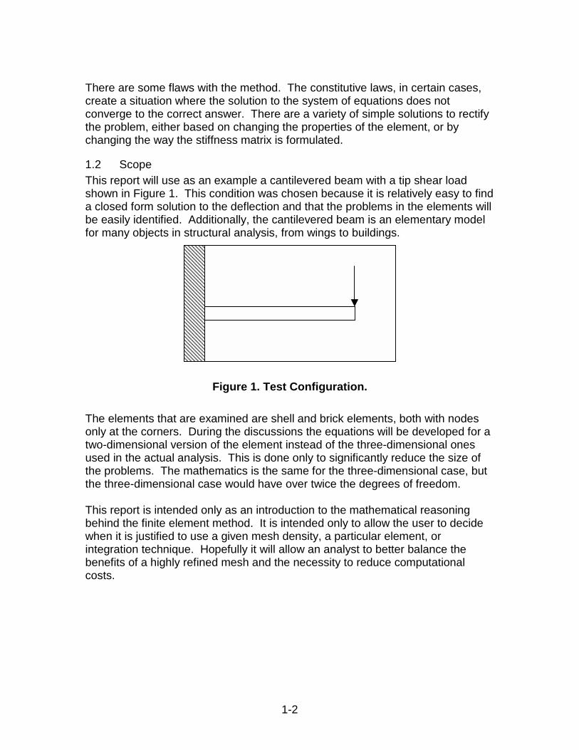
1.2 ScopeThis report will use as an example a cantilevered beam with a tip shear loadshown in Figure 1. This condition was chosen because it is relatively easy to finda closed form solution to the deflection and that the problems in the elements willbe easily identified. Additionally, the cantilevered beam is an elementary modelfor many objects in structural analysis, from wings to buildings.

Figure 1. Test Configuration.

The elements that are examined are shell and brick elements, both with nodesonly at the corners. During the discussions the equations will be developed for atwo-dimensional version of the element instead of the three-dimensional onesused in the actual analysis. This is done only to significantly reduce the size ofthe problems. The mathematics is the same for the three-dimensional case, butthe three-dimensional case would have over twice the degrees of freedom.

This report is intended only as an introduction to the mathematical reasoningbehind the finite element method. It is intended only to allow the user to decidewhen it is justified to use a given mesh density, a particular element, orintegration technique. Hopefully it will allow an analyst to better balance thebenefits of a highly refined mesh and the necessity to reduce computationalcosts.

2-1

SECTION 2 EXACT SOLUTION

This particular test configuration was chosen because it not only produces thephenomenon that we want to explore, but because it is relatively easy to find theexact form of the solution. This will prepare a baseline to which the finite elementmodels can be compared.

Two different solutions are examined. The first is the deflection solution, whichaccounts for both the bending deformation and the shear deformation. Thismethod uses the variation of total potential energy to determine the governingequations. The second is the frequency analysis, which uses Euler-Bernoulliassumptions. These assumptions should be valid for the natural frequenciesbecause natural frequencies are independent of loading conditions, so the shearloading should not matter as much in the deflection case. Further, the beam is along slender beam so the Euler-Bernoulli assumptions should be valid under anyloading condition. This method uses the summation of forces to determine anequilibrium condition.

2.1 Deformation SolutionThe deflection solution includes both the bending and the shear deformationenergy. The beam is isotropic and constant cross-section. The dimensions ofthe beam are shown in Figure 2 below. The curvature is defined as the change inrotation and the shear is defined as the difference between the slope and therotation. The total potential energy is the bending energy and the shear energyless the work done by the tip load.

Figure 2. Dimensions of Test Beam.There are several material properties that must also be known:

E – Young’s modulusG – Shear modulusν – Poisson’s ratioφ(x) – Rotation fieldu(x) – Displacement field

b

h

L

P

κ – Shear stiffnessI – Moment of inertiaP – Applied tip loadπ - Total potential energy

2-2

The first step is to simplify the equation by making it non-dimensional.

Then, the first variation is set to zero in order to find the equilibrium conditions.Integration by parts allows grouping on the variation of each field.

To set the variation to zero, each differential equation multiplied by an arbitraryvariation must be equal to zero. The boundary terms multiplied by an arbitraryvariation must equal zero at each boundary as well. This produces twodifferential equations and four boundary conditions.

We find the equilibrium positions for the unknown displacement and rotation bysolving the simultaneous differential equations subjected to the boundaryconditions. This produces the two equations for the solution shown below. The

0

0

0

0

=

=

′−=′′

=

=

η

ηφ

φφ

Lu

Lukk

1

10

:

:

=

=

−−

′

=′

′=′′

η

η

φ

φ

φ

pkLuk

BCsLuDEs

( ) ( )01

01

1

0

1

0

1

1

0

0

0

====

=

′+′+

−

′+

−−

′

+

′′

−′+

′

−′′−=

−

+

′−

′−

′′+′′=

∫ ∫

∫

ηηηη

η

φδφφδφφδφδ

ηφδηφφδφ

δηφδφφδδφδφδφ

kLukupk

Luku

dLukkud

Lukk

Lupdk

Luk

Luk

Lu

Luk

( )

( )

( )1

221

0

1

0

22

1

1

0

2221

0

22

1

21

0

1

0

22

0

2

0

2

221

21

21

21

21

21

21

21

=

=

=

=

−

+

′−

′

+′=

−

−

′+′=

−

−

′+′=

−

−+

=

∫∫

∫∫

∫∫

∫∫

η

η

η

ηφφηφπ

ηφκηφπ

ηφκηφπ

φκφπ

Lupd

Lu

Lukd

EIL

Lu

EIPLd

Lu

EILGd

EIL

LuPLLd

LuGLd

LEI

uPdxdxduGdx

dxdEI

Lx

LL

EIPLp

EILGk

Lx

2

2

=

=

=

κ

η

2-3

equations are shown in non-dimensional form, but it would be easy to convertthem to dimensional form.

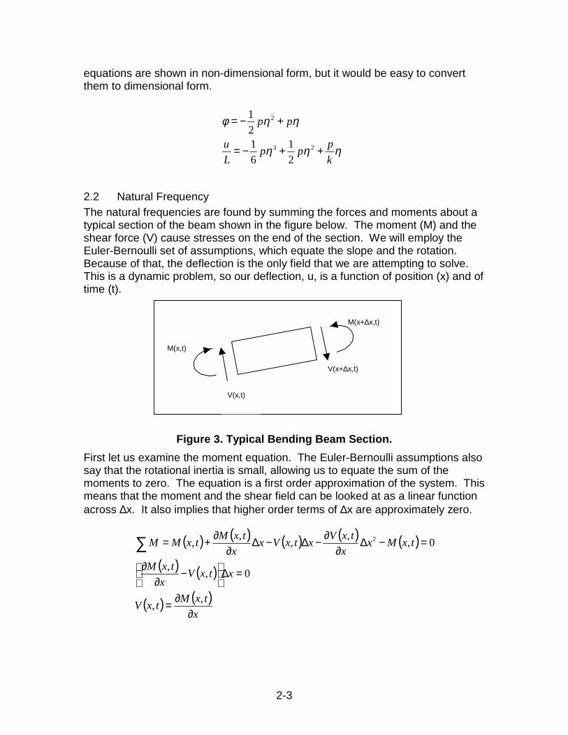
2.2 Natural FrequencyThe natural frequencies are found by summing the forces and moments about atypical section of the beam shown in the figure below. The moment (M) and theshear force (V) cause stresses on the end of the section. We will employ theEuler-Bernoulli set of assumptions, which equate the slope and the rotation.Because of that, the deflection is the only field that we are attempting to solve.This is a dynamic problem, so our deflection, u, is a function of position (x) and oftime (t).

Figure 3. Typical Bending Beam Section.First let us examine the moment equation. The Euler-Bernoulli assumptions alsosay that the rotational inertia is small, allowing us to equate the sum of themoments to zero. The equation is a first order approximation of the system. Thismeans that the moment and the shear field can be looked at as a linear functionacross ∆x. It also implies that higher order terms of ∆x are approximately zero.

ηηη

ηηφ

kppp

Lu

pp

++−=

+−=

23

2

21

6121

M(x+∆x,t)

M(x,t)

V(x,t)

V(x+∆x,t)

( ) ( ) ( ) ( ) ( )

( ) ( )

( ) ( )x

txMtxV

xtxVx

txM

txMxx

txVxtxVxx

txMtxMM

∂∂=

=∆

−

∂∂

=−∆∂

∂−∆−∆∂

∂+=∑

,,

0,,

0,,,,, 2

2-4

Next we sum the forces using the same first order approximations. This timeequating the sum of the forces to the mass times the acceleration of the section.

We combine the equations by differentiating the result of the moment equation.

The Euler-Bernoulli assumption states that the moment is equal to the bendingstiffness (EI) times the second derivative of the deflection. This comes fromequating the rotation with the slope, meaning that the curvature is the secondderivative of the deflection. We use this to reduce our differential equation to asingle time and space dependent variable.

Suitable boundary conditions need to be developed for this differential equation.For free vibrations we know that the free end will carry no shear load or moment.Using the earlier definitions for our shear and moments, and a fixed displacementand slope at the cantilevered end we get the following boundary conditions.

Using separation of variables, with λ being the separation constant, the deflectionequation becomes:

After the boundary conditions are applied, you reduce the system to twoequations and two unknowns.

( )

0

0

,

2

22

4

4

2

2

4

4

2

2

=∂∂+

∂∂

=∂∂+

∂∂

∂∂=

tuc

xu

tu

EIA

xu

xuEItxM

ρ

( )( ) 0,0

0,0

=∂

∂=

xtu

tu ( )

( ) 0,

0,

3

3

2

2

=∂

∂

=∂

∂

xtLu

xtLu

( ) ( ) ( )

( )2

2

2

2

,

,,,

tuxAx

xtxV

tuxAx

xtxVtxVtxVF

∂∂∆−=∆

∂∂

∂∂∆=∆

∂∂−−=∑

ρ

ρ

( ) ( )

( )2

2

2

2

2

2

,

,,

tuA

xtxM

xtxM

xtxV

∂∂−=∂

∂=∂

∂

ρδ

δ

( ) ( ) ( ) ( ) ( )224

4321 coshsinhcossin

cxcxcxcxcx

λβββββφ

=

+++=

2-5

To avoid the trivial solution, it is necessary to make to determinate of the matrixequal to zero. This is done by varying the values of βL. The first few values thatcreate a zero determinate are listed below. From the time dependent portion ofthe separation of variables, the frequency of oscilliation was shown to be λ.Using the material properties and the relationships shown above the βL valuesare changed into frequencies. The units are then changed from radians persecond to hertz.

βL= 1.875104 λ1= 9.7260 HzβL= 4.694091 λ2= 60.9518 HzβL= 7.854757 λ3= 170.6668 HzβL= 10.995541 λ4= 334.4388 HzβL= 14.137169 λ5= 552.8514 Hz

By changing the orientation of the beam it is easy to find the lateral bendingfrequencies. Only the first bending is low enough to be relavent to the problem.

λ lat= 194.5200 Hz

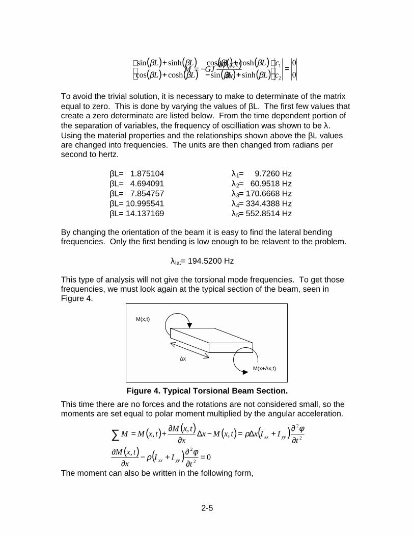
This type of analysis will not give the torsional mode frequencies. To get thosefrequencies, we must look again at the typical section of the beam, seen inFigure 4.

Figure 4. Typical Torsional Beam Section.This time there are no forces and the rotations are not considered small, so themoments are set equal to polar moment multiplied by the angular acceleration.

The moment can also be written in the following form,

( ) ( ) ( ) ( )( ) ( ) ( ) ( ) 0

0sinhsincoshcos

coshcossinhsin

2

1 =

+−+

++cc

LLLLLLLL

ββββββββ

∆x

M(x,t)

M(x+∆x,t)

( ) ( ) ( ) ( )( ) ( ) 0,

,,,

2

2

2

2

=∂∂+−

∂∂

∂∂+∆=−∆

∂∂+=∑

tII

xtxM

tIIxtxMx

xtxMtxMM

yyxx

yyxx

φρ

φρ

( )x

txGJM∂

∂−= ,φ

2-6

where J is the torsional stiffness of the beam. For a beam with a 10:1 aspectratio cross-section, such as the one in the model, J is defined as below.As in the bending case, this relationship is used to create a single field differentialequation. The boundary conditions of a one fixed end and one with no momentare also translated mathmatically.

Using separation of variables and the boundary conditions as in the bendingcase, the non-trivial solution is satisfied if λ has the following values.

βL= π/2 λ1= 89.6567 HzβL= 3π/2 λ2= 268.9700 HzβL= 5π/2 λ3= 448.2834 HzβL= 7π/2 λ4= 627.5968 HzβL= 9π/2 λ5= 806.9101 Hz

The first ten frequencies have been calculated as:

1 bend 2 bend 1 tor 3 bend 1 lat9.726 60.952 89.657 170.667 194.520

2 tor 4 bend 3 tor 5 bend 4 tor268.970 334.439 448.283 552.851 627.597

To calculate the mode shapes we need to return to the shape function. Then wecan vary βL from 0 to the value calculated above. We must also solve for eachof the four constants that appear in the equation. Unfortunately we used some ofthe information to determine the frequencies, so we still have one more unknownvariable than the number of equations. We can pick a unit value for one of theconstants and define the other by the ratio of the two. The value of the deflectionis normalized by the stiffness matrix such that the mode shape vector transposedtimes the stiffness matrix times the mode shape vector is equal to one. Theanalagous method of normalization in the exact form of the solution would be tointegrate the stiffnesses times the degrees of freedom squared over the lengthof the beam. That is more effort than the resulting benefit would yield, so onlythe unnormalized results are shown in the figure below. Also the torsional modesare more difficult to show when assumed to be a part of a one-dimensionalbeam. Therefore, Figure 5 only shows the first three bending modes.

313.0

3

==

ddbhJ

( ) ( )

( )GJ

IIc

ttxc

xtx

yyxx +=

=∂

∂+∂

∂

ρ

φφ

2

2

22

2

2

0,,( )

( ) 0,0,0

:

=∂

∂=

xtL

tBCs

φφ

2-7

Figure 5. Theory Based Bending Mode Shapes.

-3

-2

-1

0

1

2

3

0 0.1 0.2 0.3 0.4 0.5 0.6 0.7 0.8 0.9 1

3-1

SECTION 3 SHELL ELEMENT LOCKING

The first element that we will look at is the shell element. For the mathematicaldevelopment of the element, a one-dimensional model is used, but the premise isthe same as in the full two-dimensional case. The element mode shapes will bepresented in the one-dimensional case. The deflection solution was calculatedby building the beam and solving the analysis in Excel.

3.1 Element Mode ShapesThe first step that we need to accomplish when building the element is to definethe displacement field across the element. The displacement at each node mustbe completely independent of the other nodes in the element. This is done bycreating a shape function that has a value of one at one node and zero at all theother nodes. These shape functions are added together in a linear combinationwith each shape function multiplied by the value at a particular node. The shapefunctions are written with respect of the local variable r and can be seen in Figure6.

Figure 6. Shell Element Shape Functions.The displacement field can also be written in matrix form. This will be a moreadvantageous form for later work.

The next step is to define the strain field in the element. There are two types ofstrain just as it was in the development of the exact solution. The bending strainand the shear strain are defined the same way as before.

1-1

-1 1

r

r

( )121

1 += rh

( )121

2 −−= rh

( ) ( ) ( )( ) ( ) ( ) 2211

2211

φφφ rhrhrurhurhru

+=+=

( )( )

2

2

1

1

21

21

0000

φ

φφ u

u

hhhh

rru

= ( ) ( )urHru ˆ=

φφφγ

φφφ

−=−=−=

===Κ

drdu

ldxdr

drdu

dxdu

drd

ldxdr

drd

dxd

2

2

3-2

The curvature and the shear deformation can also be expressed in matrix form.The B matrix is called the strain-interpolation matrix. In this notation, the primemarking indicates a derivative with respect to the local coordinate r, and l is theglobal element length.

Expressing the our strain energy equation similarly to the exact solution form,and then converting it into matrix notation points out the form for the stiffnessmatrix described in the background portion of the introduction. J is the Jacobianmatrix expressing the transformation from the local to the global coordinates. Inthis case there is only one transformation, which was earlier expressed as l/2.

The stiffness matrix is a way of expressing the relationship between an appliedforce at one position on a structure, and the response at some other position.The relationships are assumed to be linear, letting us use the follow form for theequilibrium position. Linearity also allows us to combine several elementstogether by adding the common matrix entries for common nodes.

There are several interesting aspects to a structure’s stiffness matrix. The modeshapes that an element or structure can assume and their frequencies can befound by extracting the eigenvalues and eigenvectors from the stiffness matrix.The eigenvectors describe the displacement of each node while the associatedeigenvalue predicts the natural frequency for that mode.

The shell element has four modes, two rigid body modes and two elastic modes.The rigid body modes have a frequency of zero, while the elastic modes havenon-zero frequency. The eigenvectors are shown with normalized values thatmake the magnitude of the vector one. It is important to also note that eachmode is orthogonal to the others. Any normalized eigenvector multiplied byanother is equal to zero, while any normalized eigenvalue squared is equal toone.

2

2

1

1

2211

21

22

2020

φ

φγ u

u

hhl

hhl

hl

hl

−′−′

′′=

Κ ( ) ( )urBr ˆ=ε

( ) ( )

uKuudrJCBBuV

drlG

EIV

drlGdrlEIV

TTT ˆˆ21ˆˆ

21

200

21

221

221

1

1

1

1

1

1

21

1

2

=

=

Κ

Κ=

+Κ=

∫

∫

∫∫

−

−

−−

γκγ

γκ

FuK =

3-3

Figure 7. Shell Element Mode Shapes.

3.2 Deflection SolutionThe final solution is a linear combination of the mode shapes; each multiplied bya modal participation factor. It is easier to solve the set of simultaneous linearequations than it is to find the modal participation factors. Most times the modalparticipation factors are extraneous to the final deflection and stress results.

Demonstrating the ease of using FEM technique on simple geometry, the systemis solved for using Excel. The speed that the solution approaches the exactsolution is dramatic. Unfortunately, because of the shear locking, it will notbecome apparent until changes are made to the integration scheme.

λ1=0

λ4=1.02Ε+6

λ3=4.15Ε+6

λ2=0

02

102

1

1 =φ

683

685

683

685

2

−

−

−

=φ

210

21

0

3

−=φ

685683

685683

4 −=φ

3-4

The meshing scheme used on the beam is to divide it equally along the length ofthe beam. Cases of one, two, and three elements are inspected.

Gaussian integration is used to evaluate the stiffness matrix. By sampling alimited number of places, you can evaluate a polynomial integral exactly the overa region. The number of sampling points is determined by the degree of thepolynomial that you wish to evaluate. N sample points can exactly evaluate anintegral of (2n –1) order. The polynomial in the stiffness matrix is second orderso there must be a minimum of two sample points. The points must be thezeroes of the Legendre Polynomial. For n equal two this means that the samplepoints will be r=±3-!. There must also be a weighting factor multiplied by theresults at each sample points. For n equal two, the weight factor happens to beone for both points. This yields the following as the integrated stiffness matrix foran element length of ten.

The first two degrees of freedom are constrained to zero displacement. Thismeans when solving for the equilibrium solution it is only necessary to solve forthe last two degrees of freedom. The applied load is a point force on theunconstrained node. That makes our final system of equations the following.The same is done for the two and three element systems. The difference being

the common degrees of freedom are added together creating a banded stiffnessmatrix. The displacements are shown in the following chart compared to theexact displacements.

Number ofElements Tip Displ.

Exact 6.897098

OneElement 0.002184

TwoElements 0.008729

ThreeElements 0.019609

Figure 8. Locked Beam Displacements.

−−−−

−−

=

61031779154043050863915404915404183081915404183081

30508639154046103177915404915404183081915404183081

K

0100

6103177915404915404183081 1

2

2−

−

−=

φu

0

1

2

3

4

5

6

7

0 0.1 0.2 0.3 0.4 0.5 0.6 0.7 0.8 0.9 1

3-5

It is obvious from either Figure 7, or the table of tip displacements that the lockingphenomenon is a severe flaw in the method. It is clear something is very wrongin this simple case, but in complex loading of a shell modeled blade it would notbe as easy to determine that the shear deformation is not contributing.

3.3 Cause of LockingAn over-constrained system, or perhaps better put, an overly inflexible set ofshape functions, causes shears locking. Two linear functions only have fourunknowns to determine. After applying the four boundary conditions there are nomore unknowns to manipulate. This means that the chances that the shapefunctions will satisfy the differential equations are slim. It is easy to see thisthrough working the example we have been working.

The finite element code does not apply all the boundary conditions and then tryto satisfy the differential equations. It applies the geometric boundary conditions,then lets the natural boundary conditions come through the minimization process.Following this procedure, we start by applying the geometric boundaryconditions.

Next, the differential equations are satisfied. This produces the locking results.

The actual results are not zero displacement because the minimization processtries to impose the natural boundary conditions while solving the differentialequations. This would enforce some tip displacement, but it can be shown thatthe tip displacement approaches zero as the aspect ratio of the elementincreases.

3.4 Element ApplicabilityMost commercial packages do not use the type of integration scheme on shellelements because of the severe problems shown above. One notable exceptionis when analyzing pressure vessels. Some codes use the fact that the fullyintegrated shell element does not react to bending loads to better model the

( )

( ) 1

21

cLu

ccLu

=′

+=

η

ηη ( )( ) 3

43

ccc

=′+=

ηφηηφ

( ) ηηφ

φη

4

310

c

c

=

==′=

( ) ηη

η

1

20

0

cLu

cLu

=

===

( ) 0000

0

33

==⇒=−

=′′

−′

ηφ

φ

ccLu

( ) 0

0000

0

11

=

=⇒=−−

=′

−′′−

η

φφ

Lu

ckcLukk

3-6

steady state equilibrium of pressure vessels. The elements will only deformaxially, so surfaces will remain perpendicular to the pressure.

Otherwise codes will automatically use reduced integration. It will be shown laterthat reduced integration is an easy solution to the shear-locking problem.Reduced integration causes some other problems of which the user must beaware.

The constitutive law and strain displace relationships will enforce equilibriumwithin the element even if flawed boundary conditions provide the incorrectforces. The finite element method does not enforce equilibrium between theelements. That is why an increasing number of elements creates a bettersolution. It should be noted that it is not the correctness of the FEM that causesa finer mesh to be more exact in this case, but the flaw in the method that does.

4-1

SECTION 4 BRICK ELEMENT LOCKING

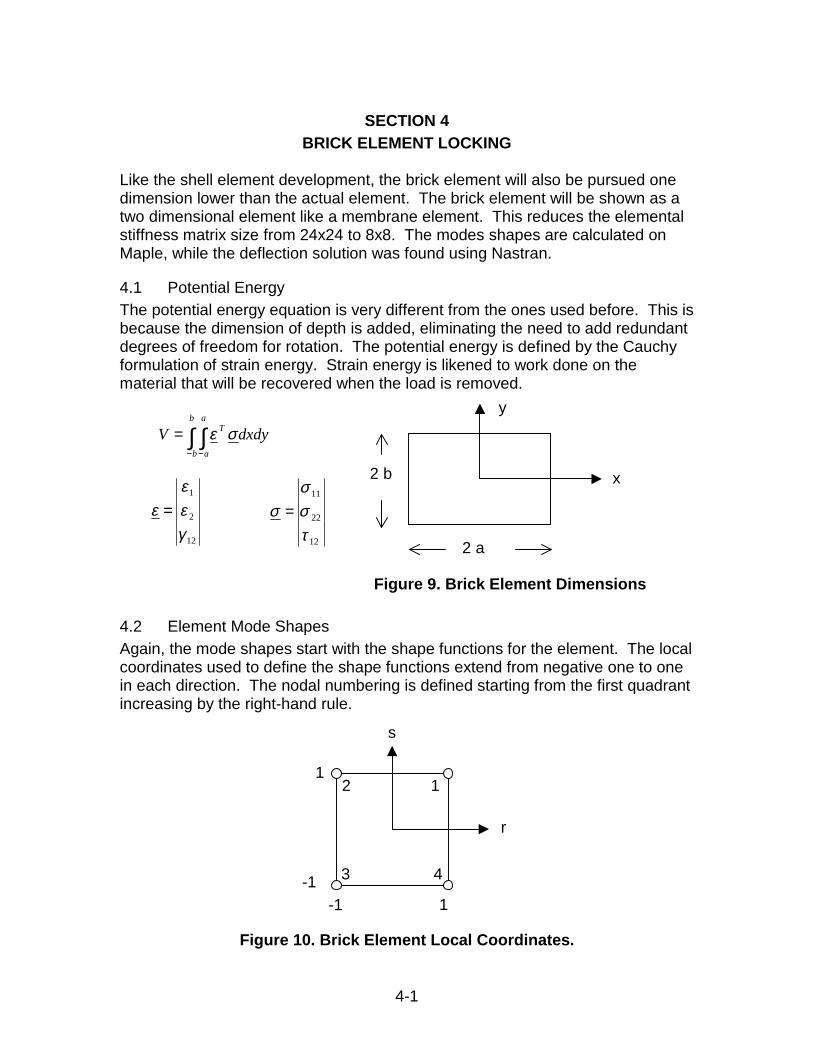
Like the shell element development, the brick element will also be pursued onedimension lower than the actual element. The brick element will be shown as atwo dimensional element like a membrane element. This reduces the elementalstiffness matrix size from 24x24 to 8x8. The modes shapes are calculated onMaple, while the deflection solution was found using Nastran.

4.1 Potential EnergyThe potential energy equation is very different from the ones used before. This isbecause the dimension of depth is added, eliminating the need to add redundantdegrees of freedom for rotation. The potential energy is defined by the Cauchyformulation of strain energy. Strain energy is likened to work done on thematerial that will be recovered when the load is removed.

Figure 9. Brick Element Dimensions

4.2 Element Mode ShapesAgain, the mode shapes start with the shape functions for the element. The localcoordinates used to define the shape functions extend from negative one to onein each direction. The nodal numbering is defined starting from the first quadrantincreasing by the right-hand rule.

Figure 10. Brick Element Local Coordinates.

∫ ∫− −

=b

b

a

a

T dxdyV σε

12

2

1

γεε

ε =

12

22

11

τσσ

σ =

2 b

2 a

x

y

r

-1

s

1-1

1

4

2 1

3

4-2

The shape functions have a unit value at the node of interest, and zero values atall other nodes. A typical shape function is shown after the shape functionsbelow.

Figure 11. Brick Element Shape Function.The next step is to define the strain-displacement relationship. The differencesfrom the shell element are axial strain in two dimensions and that the shear strainis defined differently. The k index in the matrix notation is to denote the shapefunction number. The strain interpolation matrix will be a three by eight matrix inthis example.

The final ingredients needed to find the stiffness matrix, and then the modeshapes, are the constitutive laws. The plane stress relationships are used todefine the connection between the strain and the stress.

( )( )

( )( )srh

srh

+−=

++=

1141

1141

2

1( )( )

( )( )srh

srh

−+=

−−=

1141

1141

4

3

dxdr

drdv

dyds

dsdu

dxdv

dydu

dyds

dsdv

dydv

dxdr

drdu

dxdu

+=+=

==

==

12

2

1

γ

ε

ε

u

ha

hb

hb

ha

rksk

sk

rk

ˆ

11

10

01

,,

,

,

12

2

1

= ΛΛγεε

12

2

1

2

12

22

11

2100

0101

1γεε

νν

ν

ντσσ

−−= E

h1

4-3

The Jacobian becomes a more complex matrix because of the second dimensionadded to the problem. The Jacobian is defined in the following manner. TheJacobian is used to transform the coordinates from the global to the elementalcoordinates.

Combining all the relationships into the strain energy equation will produce thestiffness matrix, just as it did for the shell element. The same notation applies asbefore. The B matrix is the strain interpolation matrix. The matrix used in theconstitutive law is the C matrix.

The stiffness matrix for this element is an eight by eight matrix. This means therewill be eight mode shapes. There are three rigid body modes, two translationsand one rotation. There are five elastic modes, one uniform, two shear, and twobending modes. All of the modes are shown below with the associatedeigenvalue. The rigid body modes have a zero eigenvalue, meaning that they allmust be constrained or the stiffness matrix will be singular.

Horizontal Translation Vertical Translation Rotationλ=0 λ=0 λ=0

Figure 12. Brick Element Rigid Body Modes.

dsdr

Jdydx

dsdr

dsdy

drdy

dsdx

drdx

dydx

=

=

( )

( )

uKuudrdsJCBBuV

dxdyuCBBuV

dxdyV

TTT

b

b

a

a

TT

b

b

a

a

T

ˆˆˆˆ21

ˆˆ21

21

1

1

1

1

=

=

=

=

∫ ∫

∫ ∫

∫ ∫

− −

− −

− −

σε

4-4

Bending Bending Uniform Contractionλ=0.4976 λ=0.4976 λ=1.47

Uniaxial Shearλ=0.7575 λ=0.7575

Figure 13. Brick Element Bending Modes.

4.3 Deflection SolutionPatran generated the code to analyze the deflection solution in Nastran. Therewere two models used. The first model had 180 elements, each with eightnodes. The elements each had a length and width of a third and were one-tenthinch deep. This model is shown in Figure 14. The other model had the samedimensions, but the elements were one-fifth inch long and wide.

Figure 14. Brick Element Beam Model.Both beams are held to the same boundary conditions. At one end of the beamthe end nodes were set to zero displacement out of the plane. The center two

6 elements

30 elements

0.3330.333

0.1

4-5

nodes were additionally held to no displacement within the plane either. Theother end had a 100-pound downward force applied to the upper center node.

There are several different integration methods that can be used by Nastran toevaluate the stiffness matrix. The option used in this model told Nastran to usefull integration to evaluate the stiffness matrix. This meant for two gauss pointsto be used in each direction in obtaining the exact solution since one linearequation multiplied by another creates a quadratic equation. As in the shellelement, full integration under shear loading creates locking.

Figure 15. Locked Brick Element Deflection Solution.Even with fifty elements along the span of the beam, the deflection is only aboutone-third of what the exact solution is. This shows that although the model willstill converge to the correct solution through the discontinuity of equilibrium, theefficiency of the method is dramatically reduced.

4.4 Natural FrequenciesUsing the same integration scheme, but using a modal analysis instead of alinear analysis, Nastran will give the first ten modes and their associatedfrequencies. These are compared to the calculated values in the table below.

FEM Calculations Error1 lateral 188.48 194.52 -3.11%1 torsion 99.24 89.66 10.69%2 torsion 311.76 268.97 15.91%3 torsion 563.24 448.28 25.64%4 torsion 872.36 627.60 39.00%1 bend 16.34 9.73 67.97%2 bend 102.29 60.95 67.82%3 bend 285.75 170.67 67.43%4 bend 559.20 334.44 67.21%5 bend 922.83 552.85 66.92%

The locking effect’s dependence on the aspect ratio of the element and thestructure is clear. In the lateral deflection, the structural length (10) divided depth(2) is five, while in the bending direction, the quotient (10/0.1) is 100. The error is

0

1

2

3

4

5

6

7

0 0.1 0.2 0.3 0.4 0.5 0.6 0.7 0.8 0.9 1

180 ElementsExact500 Elements

4-6

approximately twenty times greater as is the quotient. Further, the element hasan aspect ratio of over three to one for the bending mode and just one to one forthe lateral bending.

The percent error is also dependent on the mode shape number. Some modeshave different amounts of curvature in each direction. The more curvature that isrequired, the more error there will be in general. The bending modes are allsimilar in error, potentially because it is the maximum error limit.

4.5 Cause of LockingThe element locks because it is an inflexible system just as the shell element is.The definition of linear is a little different in these shape functions, creating amore flexible system, but even this added flexibility is not enough to unlock thesystem. The existence of four nodes implies that we will need four coefficients tocorrectly determine the system. Unfortunately, two linear functions ofindependent variables only have three coefficients when combined since theconstants can be added together. This is how a non-linear term gets added intothe linear shape functions shown below.

Just as in the example with the shell element the brick element is subject to bothgeometric and natural boundary conditions. Each displacement field has one ofeach type at both ends of the element. Take as an example the element with thecoordinate axes shifted to the position shown below to make the equations moreeasily examined. The single equation requiring no displacement in the udirection acts as two separate constraints at x=0.

but because the equation must hold forall values of y the only solution is:

Figure 16. Brick Element with Shifted Axes.Likewise, the boundary conditions on the other end relating deflection to theapplied shear also add four constraints. These eight constraints combined withtwo differential equations create a total of ten constraints and only eightunknowns. The system is over-constrained and tends toward the trivial solutiontrying to satisfy all conditions.

( )( ) 8765

4321

,,

cxycycxcyxvcxycycxcyxu

+++=+++=

x

y ( )( ) 0,0

0,0

86

42

=+==+=

cycyvcycyu

00

6

2

==

cc

00

8

4

==

cc

5-1

SECTION 5 SHELL ELEMENTS WITH REDUCED INTEGRATION

Locking needs to be removed in order to predict the stress correctly anddisplacement fields in some structures. There must be changes made to theelement to have it work correctly. There are two main ways to this: change thedegrees of freedom to match the number of constraints or modify how thestiffness matrix is built so that the constraints can be followed with the samenumber of degrees of freedom.

The number of degrees of freedom is dependent on the number of nodes. Byintroducing a node at the mid-span point of the element, two additional degreesof freedom are introduced. This brings the total to three translations and threerotations, equaling the constraints. There is no locking in this new element. Thisis similar to the method followed in the brick element with a bubble mode.Changing the shape functions to a higher order polynomial increases the numberof constants that must be solved for to at least equal to the number ofconstraints.

We will leave that for the next section and now see what can be done if there is aneed to use a two-node element instead of the one with three nodes. If thestiffness matrix is determined by using a lower order Gaussian integration theelement will no longer have locking. This section will focus on this reduced orderintegration technique.

5.1 Mode ShapesThe shape functions will still be linear for this analysis. This makes the functionto be integrated a second order polynomial when the shape functions aremultiplied together. To exactly evaluate a second order polynomial would requiretwo Gauss points. For this analysis we only use one Gauss point.

This changes the values of the stiffness matrix and therefore possibly theeigenvalues and eigenvectors. The overall eigenvectors do not change, but aneigenvalue does change. The bending mode has an eigenvalue that waslowered by three orders of magnitudes. This means that the amount of energythat is needed to cause a change in the deflection is much less than the lockingsituation, allowing the locked configuration to unlock.

The reduced order integration will exactly integrate the equations in the stiffnessmatrix, except for those in the second or fourth column and the second or fourthrow. That is because when the strain interpolation matrix is transposed andmultiplied by itself, only those positions have a term of r squared. This isapparent when we recall the strain interpolation matrix that was developed beforeis as shown below.

5-2

The only mode shape that is completely defined by the stiffness in the rotations isthe fourth mode. It is also the only mode that changes eigenvalues. All othereigenvalues are based on the stiffness of either, combined rotation andtranslation (odd column and even row and vice versa), or pure translation (oddrows and columns).

5.2 Force-Displacement MatrixThe construction of the stiffness matrix through full integration of the constitutiveequations and the strain displacement relationship effectively minimizes theunknown constants in the deflection solution in a given ratio in accordance withthe governing laws. The matrix inversion and the applied forces then solve forthe magnitude of that ratio by creating a linear combination of those deflectionratios. This is obvious when you view the equation.

0.001912 0.001147 0.005732 0.001147 0.009552 0.0011470.001147 0.000689 0.003441 0.000689 0.005736 0.0006890.005732 0.003441 0.019103 0.004589 0.034383 0.0045890.001147 0.000689 0.004589 0.001378 0.009177 0.0013780.009552 0.005736 0.034383 0.009177 0.066854 0.0103240.001147 0.000689 0.004589 0.001378 0.010324 0.002067

The inverse of the stiffness matrix is clearly a way to combine the individualshape functions. To represent this, the figure below shows the deflection for aunit force applied at a particular node. The final solution is a linear combinationof each of these shapes, each with the participation coefficient equal to the loadapplied at the respective node.

Figure 17. Beam Deflection Mode Shapes.

( ) ( )2

2

1

1

12111

211

1010

φ

φγ u

u

rl

rl

ll

+−−−

−

=Κ ( ) ( )urBr ˆ=ε

FKd 1−=

0

0.01

0.02

0.03

0.04

0.05

0.06

0.07

0 0.1 0.2 0.3 0.4 0.5 0.6 0.7 0.8 0.9 1

Force at Node 1

Force at Node 2

Force at Node 3

=K-1

5-3

The first thing that can be seen is that the unit force creates a greaterdisplacement when applied at a more outboard node. This makes sensebecause it would create a greater moment about the beam root.

The inverted stiffness matrix also shows that the strain-displacementrelationships are enforced. This is best seen in the first column representing aload applied at the first node. The rotation at all further nodes are equal to therotation at the first node. This is because the beam’s curvature is proportional tothe moment at that point. Outboard of the applied force there is no reactionforce, nor reaction moment. This means that curvature outboard should be zeroimplying a constant rotation and slope. Both of these implications are found tobe true in the graph above.

5.3 Deflection SolutionThe difference that this makes in the final solution is drastic. The effect ofmaking the change in rotation easier makes the solution converge towards theexact solution very quickly.

Once again the solution was done on Excel. The stiffness matrix was inverted byusing the row-echelon format. The inverted matrix multiplied by the force vectorwill produce the deflection solution. The solution is found for one, two, and threeelements across the length of the beam. Solutions are compared both in thegraph and in the table of tip displacements.

Number ofElements Tip Disp.

Exact 6.897098

OneElement 5.17296

TwoElement 6.466063

ThreeElement 6.705527

Figure 18. Reduced Integration ShellDeflection Solution.

The elements are more accurate as the actual deflection approaches a linearfunction. When there is more curvature in the solution the elements must besmaller to stay close to the exact answer. Even so, the error is small consideringthere are only three elements. In fact, the solution converges to the exactsolution very quickly. Remember that the locked solution yields a zero deflectionsolution for high aspect ratio elements such as these.

0

1

2

3

4

5

6

7

0 0.1 0.2 0.3 0.4 0.5 0.6 0.7 0.8 0.9 1

exact

1 elem.

2 elem.

3 elem.

5-4

The effect the change has on the rotation is more curious. The reduced energyto cause rotation allows the tip rotation to equal the exact for any number ofelements, including only one. Therefore the stiffness matrix applies the tipmoment boundary condition exactly.

5.4 Natural FrequenciesTo find the first ten natural frequencies of the system there must be at least tendegrees of freedom. This means that you would need to invert at least a ten byten matrix, more if you wish to have more accuracy. This makes the reverseechelon method impractical. Instead, Nastran solved the system of equations.

For this example a system of 80 four-node shell elements predicted thefrequencies. The beam had four elements across the width and twenty along thelength. A figure showing the mesh is located below.

Figure 19. Meshing of Reduced Order Shell Elements.The higher number of elements attempts to keep the curvature close to zeroacross any given element. This will reduce the error in energy in a given modeand make the frequency closer to the exact frequency. The improvement of thefrequency prediction over the locked brick elements is apparent. These could beimproved by adding more elements. They would be best added across the widthto rectify the error in the torsion modes.

FEM Calculations Error1 lateral 188.42 194.52 -3.14%1 torsion 90.79 89.66 1.26%2 torsion 276.92 268.97 2.96%3 torsion 476.23 448.28 6.23%4 torsion 696.26 627.60 10.94%1 bend 9.85 9.73 1.23%2 bend 61.50 60.95 0.90%3 bend 172.12 170.67 0.85%4 bend 337.46 334.44 0.90%5 bend 557.91 552.85 0.98%

The higher order torsion modes have the most error because they havecomponents of curvature in both the length and width directions. The higher themode the more nonlinear the deflection is across a given element, causing theerror to increase as the modal number increases.

5-5

5.5 Element Applicability and Meshing CriteriaThis element is a good one to use in most situations. It is the only integrationtechnique used by most codes for shell elements. The major limitation to thereduced integration techniques is that it cannot be used when the stiffness ormass matrix is not symmetric. So, if there is an active control system or energylosses not associated with damping forces the reduced integration technique willnot work.

The best method of meshing is to have as many elements as possible across thestress gradient, the steeper the stress gradient the more elements required. Inour example the stress gradient lines run across the width of the beam. Thisimplies that for best results single elements could run across the width of thebeam, giving the most possible elements across the stress flow.

In most cases the stress gradient is not known before the analysis. The bestidea is to then keep the elements close to an aspect ratio of one to get an initialmesh. After the general stress field is known a refined mesh can be created.

There will always be a tradeoff between the increase in accuracy and theincrease in computational costs. The increase of computational time is roughproportional to the number of elements squared. Ultimately the solution to thistradeoff is left to the analyst.

6-1

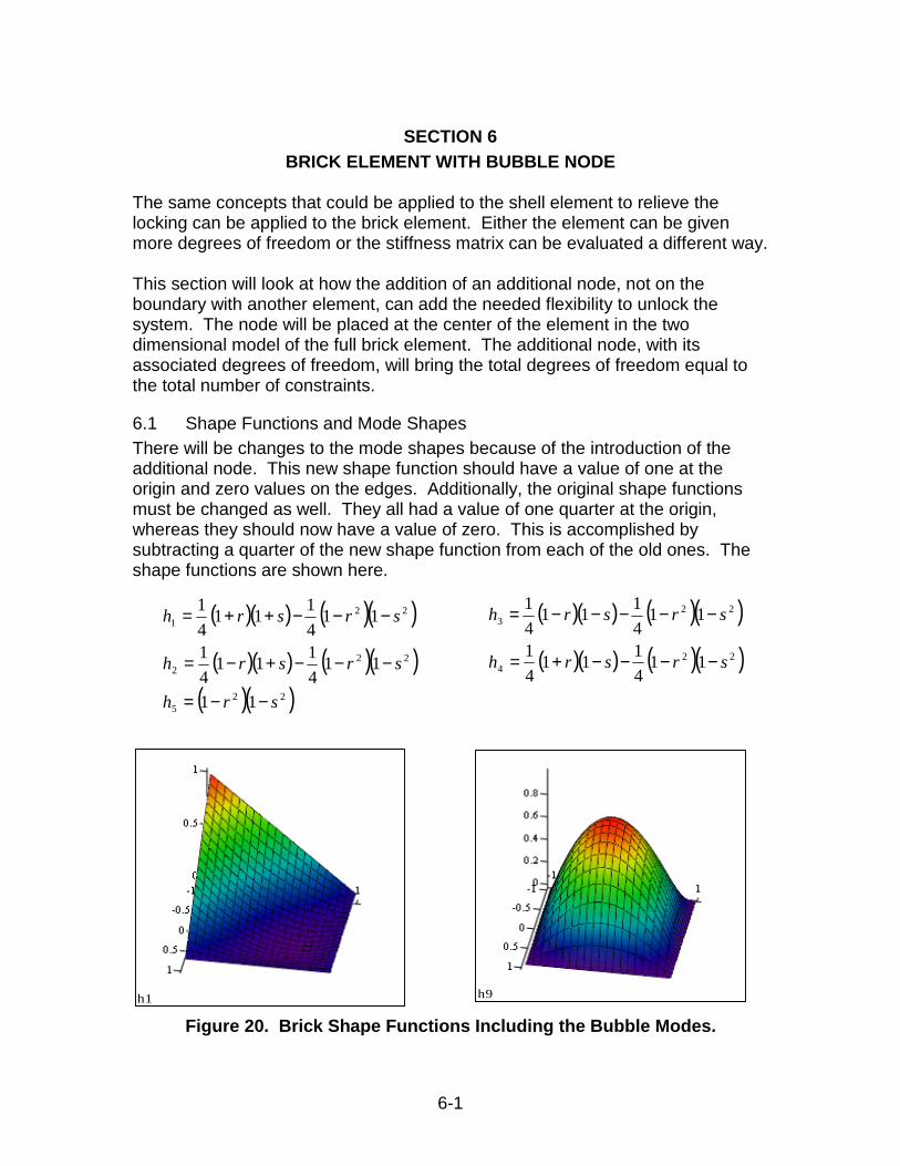
SECTION 6 BRICK ELEMENT WITH BUBBLE NODE

The same concepts that could be applied to the shell element to relieve thelocking can be applied to the brick element. Either the element can be givenmore degrees of freedom or the stiffness matrix can be evaluated a different way.

This section will look at how the addition of an additional node, not on theboundary with another element, can add the needed flexibility to unlock thesystem. The node will be placed at the center of the element in the twodimensional model of the full brick element. The additional node, with itsassociated degrees of freedom, will bring the total degrees of freedom equal tothe total number of constraints.

6.1 Shape Functions and Mode ShapesThere will be changes to the mode shapes because of the introduction of theadditional node. This new shape function should have a value of one at theorigin and zero values on the edges. Additionally, the original shape functionsmust be changed as well. They all had a value of one quarter at the origin,whereas they should now have a value of zero. This is accomplished bysubtracting a quarter of the new shape function from each of the old ones. Theshape functions are shown here.

Figure 20. Brick Shape Functions Including the Bubble Modes.

( )( ) ( )( )

( )( ) ( )( )( )( )22

5

222

221

11

114111

41

114111

41

srh

srsrh

srsrh

−−=

−−−+−=

−−−++= ( )( ) ( )( )

( )( ) ( )( )224

223

114111

41

114111

41

srsrh

srsrh

−−−−+=

−−−−−=

h9h1

6-2

The new shape function will increase the size of the stiffness matrix to a ten byten matrix. This means that there are now ten eigenvalues and ten eigenvectors.The original eight are the same, but the two new ones are associated with thebubble node. These are called bubble modes because they are primarily adisplacement of the bubble node without much deflection in the other modes.

The mode shapes remain the same for the stiffness matrix including the bubblenode. The only change beside the addition of the bubble modes is the loweringof the bending modes’ eigenvalue. This is evidence that the bending stiffness ofthis element is reduced. The modes and their eigenvalues are displayed in thefigures below.

Shearing Uniaxial Tension Biaxial Tensionλ=0.7575 λ=0.7575 λ=1.47

Figure 21. Brick Element Constant Strain Modes.

Vertical Bending Horizontal Bendingλ=0.389 λ=0.389

Figure 22. Brick Element Bending Modes.

Vertical Bubble Mode Horizontal Bubble Modeλ=5.4165 λ=5.4165

Figure 23. Brick Element Bubble Modes.

6-3

Rotation Horizontal Translation Vertical Translationλ=0 λ=0 λ=0

Figure 24. Brick Element Rigid Body Modes.

6.2 Solution TechniqueThe solution starts with assuming a shape function of the solution. The solutionis quadratic in the horizontal and the vertical coordinates, as well as theircombination. The new shape functions are shown below. Notice how there is aquartic polynomial term. It is included in the same manner that the quadraticterm was included in the original brick development.

These new shape functions are associated with eighteen unknown constants. Inthe same manner as explained in the section on why the brick elements lock, thetwo boundary conditions each impose three constraints on each of the newshape functions. Excluding the two differential equations, there are twelveconstraints. This leaves six constants to be solved for by the differentialequations. The equations might not be solved for exactly, but the answer can bemuch more accurate than when there was only one degree of freedom that couldbe solved for in the two differential equations.

Figure 25. Bubble Mode Element Deflection.

2218

217

216

215

21413121110

229

28

27

26

254321

yxcxycyxcycxcxycycxccvyxcxycyxcycxcxycycxccu

++++++++=

++++++++=

0

1

2

3

4

5

6

7

0 0.1 0.2 0.3 0.4 0.5 0.6 0.7 0.8 0.9 1

180 ElementsExact500 Elements

6-4

The integration of the stiffness matrix during its formulation minimizes the errorover the examined structure. This produces a deformed position that mostaccurately enforces all the boundary conditions as well as the differentialequations. The linear static solution with the mesh described using fullyintegrated bubble modes shows a tip deflection of 6.73865. This is within 2.3%of the theoretical solution, a vast improvement over the elements without thebubble mode.

6.3 Matrix InversionA difficult part of solving a linear set of equations is that there can be n unknownsin n equations, where n can be very large. To solve for any particular variable, itis necessary to have one equation and one unknown. Two common ways ofaccomplishing this is to invert the matrix, thereby lumping all unknowns into onelarge unknown, and substituting equations which require a symbolic processor,but do yield a series of one unknown equations.

A good representation of the second part of the substitution method is shown inthe following equations. Each equation only uses the values of the precedingequations plus an additional unknown. The first two equations solved for theunknowns are shown as well. The pattern is evident and easily repeatable.

Finite element packages use this process to solve systems of equations becausethey are much faster than computing the inverse of a large matrix. Unfortunately,they must solve a system that is not of the form of a lower triangular matrix.There is a way to represent any square matrix as two triangular matrices and adiagonal matrix, and a symmetric matrix as a triangular matrix and a diagonalmatrix. This method is shown in the equations below.

3

2

1

3

2

1

333231

2221

11

000

ccc

xxx

LLLLL

L=

−=

=

11

1212

222

11

11

1Lc

LcL

x

Lc

x

=

=

=

1

01001

2

23

1

13

1

12

32313

23212

13121

DK

DKDK

L

LDLDKKKDKKKD

K T

=

3

2

1

000000

DD

DD

6-5

Now a single fully populated linear matrix equation can be solved by three simplelinear equations.

substituting

substituting

solve for unknown vector

This might seem more complicated because three systems of equations must besolved instead of a single system, but they are much easier systems to solve.They also have an added benefit when dealing with a highly banded matrix asfound in finite element applications. None of the matrices lose their bandedness,unlike the inverse of a banded matrix. The inverse of a banded matrix isnormally a fully populated matrix which would take too much memory to performcalculations on it. For example, a ten thousand-degree of freedom system wouldhave to have 100 megabytes of memory simply to hold the matrix in memory, letalone perform operations on it. The simple beam model shown above with 180elements had 1260 degrees of freedom and would have needed about 1.6megabytes of memory to hold the inverted matrix.

6.4 Natural FrequenciesThe following model determined the natural frequencies of the system usingPatran. It is the same 180-element model described above comprised of Hex8brick elements.

Figure 26. Patran Model Used to Determine Natural Frequencies.The following table shows the frequencies determined by the finite elementanalysis. The accuracy is very good in the bending modes but falls off in thetorsion modes. Partly this is because of the higher strain energy in those modes.That can also be seen in the higher order bending modes, although those haveno stress gradient in the x direction.

xuL

yxD

yuDL

FyLFuLDL

FuK

T

T

T

=

=

=

==

=

uDLy T=

uLx T=

6-6

FEM Calculations Error1 lat 189.88 194.52 -2.39%1 tor 94.28 89.66 5.16%2 tor 288.27 268.97 7.18%3 tor 497.92 448.28 11.07%4 tor 732.00 627.60 16.64%1 bend 9.86 9.73 1.41%2 bend 61.70 60.95 1.22%3 bend 173.13 170.67 1.44%4 bend 340.64 334.44 1.85%5 bend 565.60 552.85 2.31%

The mode shapes can also be shown as part of the results in finite elementanalysis. Below are several of the mode shapes that are part of the solution.

Figure 27. First Bending and First Lateral Bending Modes.

Figure 28. First Torsion and Second Bending Modes.

Figure 29. Third Bending and Second Torsion Modes.These modes compare well to the shapes that were calculated in the theorecticalcase. The enforcement of the boundary conditions, both the natural andgeometric, is clear. The enforcement of the zero displacments and rotations isvisible on the root end. The zero curvature (zero moment) condition can be seenin each mode on the free end. It is harder to see the zero shear condition, but

6-7

the free face of the beam remains perpendicular to the edges leading to the endface.

6.5 Element Applicability and Meshing CriteriaIt is interesting to note that the model run with the shell elements with reducedorder integration had more accurate results with fewer elements. This isbecause the theory of plates is based on the same stress strain relationship thatthe shell elements use.

Solid elements are much more useful when there is a nonuniform thickness or ifthere is a dramatic stress gradient through the thickness caused by forces otherthan bending. It is much easier to correctly vary the thickness of the solidelements along a span than on the shell elements. Additionally, it is possible toput more than a single layer of elements through the thickness unlike in shellelements.

Although the element is no longer as susceptible to being overly stiff, this doesnot mean that the aspect ratio of the elements does not matter at all. It is stillimportant to keep the brick as close to a perfect cube as practical for a givensituation. This is because multiplying the formulation by the determinate of theJacobian forms the stiffness matrix. If the element is very skewed, thistransformation into the local coordinates is not as accurate. To keep the error toa minimum the skew of element must be at a minimum practical level. In ourexample it would be best to have all elements a cube 0.1 on each edge. Thiswould unnecessarily increase the mesh to 2000 elements. As long as theelement edges remain normal the aspect ratio can be left higher than 1.

7-1

SECTION 7 BRICK ELEMENT WITH REDUCED INTEGRATION

The final element that we will look at is the brick element with reducedintegration. There is no bubble mode, so the element is comparable to thereduced integration shell element. The element still uses the brick elementdefinition of the strain energy.

The same formulations of the strain energy and stress-strain relationship areused. Just as we used a single integration point in the reduced shell integration,there will only be one integration point in each of the local coordinate directions.

Mode shapes are not changed by reduced integration, although the associatedeigenvalues are. These new eigenvalues dramatically change the energyrequired to deform the structure, bringing the solution towards the exact solution.

7.1 Mode ShapesThe reduced order integration technique changes the associated eigenvalues forsome mode shapes. These are caused by the modification of the stiffness matrixwhen reduced order Gauss point integration incorrectly evaluates it. The theoryis the same as it is in the shell elements; the changes allow the correct mode todeform with less energy being used by the same deflection.

This theory works, but not as well as in the shell element. The main reason thatit is worse than the shell element is that the eigenvalue is reduced to zero insteadof some new positive value. Both were similar in that only the bending modeswere effected. The goal was to reduce the energy required to excite thesemodes, so the method worked well in that respect.

7.2 Deflection SolutionThe change is apparent in the solution. The solution quickly approaches theclosed form solution. An interesting thing happens as the number of elements isreduced to just a couple elements. The zero eigenvalues of the bending modesprevent the stiffness matrix from being inverted. After a few of the elements areconnected the complete system can no longer exhibit a single bending mode, sothe matrix is no longer singular. The individual elements still have zero energyassociated with their bending so the solution will not be exact. All strain energyis based on the other elastic modes although the solution shows primarilybending. The convergence is close to the exact solution, but it is not as close asthe bubble mode solution.

If the elements do not converge to the correct solution, they do converge quickly.The difference between 30 spanwise elements (180 total elements) and 50spanwise elements (500 total) is negligible.

7-2

Figure 30. Reduced Integration Defection Solution

7.3 Natural FrequenciesThere is also an associated system frequency change with the new elements.Much like the deflection solution, the frequencies come closer to the exactsolution, but not as close as the bubble functions. Depending on the applicationthe frequencies may not be close enough to accept. They still have about ten-percent error in the low frequency modes.

FEM Calculations Error1 lat 190.43 194.52 -2.10%1 tor 94.88 89.66 5.83%2 tor 291.17 268.97 8.25%3 tor 506.14 448.28 12.91%4 tor 749.94 627.60 19.49%1 bend 10.59 9.73 8.88%2 bend 66.16 60.95 8.54%3 bend 186.05 170.67 9.01%4 bend 367.41 334.44 9.86%5 bend 612.33 552.85 10.76%

0

1

2

3

4

5

6

7

0 0.1 0.2 0.3 0.4 0.5 0.6 0.7 0.8 0.9 1

180 ElementsExact500 Elements

7-3

The error in frequency stems from the same cause as the error in the deflection.The system has the incorrect energy associated with the given deflection modes,changing the amount of energy (frequency) required to excite a given mode.

7.4 Comparison with Bubble NodeThe solution is not as accurate as the bubble mode in this solution. That isbecause instead of making the model more accurate by increasing the order ofthe shape functions to better enforce the strain displacement relationship, themost prominent deflection mode has the eigenvalue arbitrarily reduced. It doesmake sense that if a system should bend and it doesn’t, reducing energyassociated with the bending mode will make the system approach the correctvalue. The problem is that a better solution comes from the degradation of themodel and not from a more exact model.

Another way to look at the solution is to say that the shape functions are a seriesof normal functions added together. As the number of normal functionsincreases, the solution approaches the exact solution as in the Fourier Seriesexpansion of a function. It can be shown that increasing the polynomial order ofthe shape function will bring the solution closer to the exact solution. That is thetheory behind p-elements, which increase the order of the polynomial shapefunction until the solution converges within a given tolerance.

Conversely, the reduced order integration has no proof that the mesh will evenconverge to the right solution let alone a more accurate one than a fullyintegrated one. In practice it does converge towards the correct solution most ofthe time, but the analyst should be aware that there is no guarantee that it will.

The reason that the bending mode eigenvalue goes to zero using reducedintegration is that the single Gauss point is at a zero strain position in theelement. That means that it will have zero energy and a zero eigenvalue. Thiscan be seen in the figure below.

Figure 31. Gauss Point Location in Reduced Order Bending Mode.

In the figure you can also see the locations of the fully integrated Gauss points bythe intersection of the dashed lines. It is clear that they are on lines that deform,and therefore have an energy associate with that deflection.

The single Gauss point in thecenter of the element islocated in the middle ofsymmetric deflection sothere is no strain at thatpoint.

8-1

SECTION 8 CONCLUSIONS AND RECOMMENDATIONS

The goal of any structural analysis is to correctly predict the conditions that willexist in a given structure. The best way to accomplish this when using theseelements that are subject to being over stiff is to understand what the differentelement property choices mean mathematically in the model.

The reduced integration technique works well in the shell method because thebending strain definition is:

and phi prime is a non-zero constant at the Gauss point. This implies that therewill be a non-zero eigenvalue associated with the bending mode because there isstrain at the Gauss point.

In the brick element, the Gauss point is at a saddle point. The values of thegradients in both the r and the s directions are zero at the Gauss point, as are theshear gradients. This means that the strain at the Gauss point is zero and willproduce a zero eigenvalue. The saddle point can be seen in the figures showingu deflection in a bending mode.

Figure 32. Deflection Plot of Bending Mode Shape.The main difference is again due to the difference in the strain energy definition.The Cauchy formulation used in the brick element is not accurate in theseconditions dominated by bending and shear.

The reduced order shell element is the best solution for overcoming locking in theshell element because the stiffness of the bending mode is not reduced to zero.

( )2φ′EI

h h

8-2

It is the best formulation of the element to use in most conditions. The analystshould still be aware that there is still no method to know that the solution that themodel converges to is the exact solution, but in most cases it is closer to realitythan the fully integrated element.

The best brick element formulation to use is the element that has quadraticshape functions. That means that the simplest element would be the eight-nodeelement using bubble functions. Other elements that also use the quadraticshape functions are the 20, 21, 26, and 27 node elements. These willdramatically increase the computational time if the number of elements remainsconstant.

Modern FEA code provides hourglass mode stiffening. This is a change in thestiffness matrix that can provide stiffness to those modes that normally wouldhave a zero eigenvalue under reduced integration. This is another solution to theproblems associated with reduced integration of brick elements.

Whatever formulation and elements used in the FEM, it is very important that theperson using them knows how and why they act as they do. An analysis is onlyas good as the method used, so knowing that you are using the right method forthe particular analysis is extremely important.