Worcester Polytechnic InstituteDigital WPI

Interactive Qualifying Projects (All Years) Interactive Qualifying Projects

April 2019

Forex Trading Systems: An Algorithmic Approachto Technical TradingAndrew VanOstenWorcester Polytechnic Institute

Benjamin John AndersonWorcester Polytechnic Institute

Nicholas Sylvester NugentWorcester Polytechnic Institute

Thar Min HtetWorcester Polytechnic Institute

Follow this and additional works at: https://digitalcommons.wpi.edu/iqp-all

This Unrestricted is brought to you for free and open access by the Interactive Qualifying Projects at Digital WPI. It has been accepted for inclusion inInteractive Qualifying Projects (All Years) by an authorized administrator of Digital WPI. For more information, please contact digitalwpi@wpi.edu.

Repository CitationVanOsten, A., Anderson, B. J., Nugent, N. S., & Min Htet, T. (2019). Forex Trading Systems: An Algorithmic Approach to TechnicalTrading. Retrieved from https://digitalcommons.wpi.edu/iqp-all/5407

brought to you by COREView metadata, citation and similar papers at core.ac.uk

provided by DigitalCommons@WPI

Forex Trading Systems:

An Algorithmic Approach to Technical Trading

An Interactive Qualifying Project

Submitted to the Faculty of

WORCESTER POLYTECHNIC INSTITUTE

In partial fulfillment of the requirements for the

Degree of Bachelor of Science

By

Benjamin Anderson (REL 1804)

Thar Min Htet (REL 1802)

Nicholas Nugent (REL 1810)

Andrew VanOsten (REL 1808)

Date: April 24, 2019

Submitted to:

Professors Reinhold Ludwig and Gbetonmasse Somasse of Worcester Polytechnic Institute

This report represents work of WPI undergraduate students submitted to the faculty as evidence of a degree requirement. WPI routinely publishes these reports on its web site without editorial

or peer review. For more information about the projects program at WPI, see http://www.wpi.edu/Academics/Projects

Abstract In financial trading, emotion can often obstruct clear decision making. The goal of this

project is to build a system which can overcome this by trading foreign currencies autonomously. Three systems were created: two relying on neural networks, and a third on pattern recognition of candlestick charts. A fourth system has been designed to allocate funds to the others using utility theory. Though the algorithms were not profitable, a powerful interface was built, connecting Python scripts to MetaTrader 4 for trading.

1

Acknowledgements

We would like to thank Professors Reinhold Ludwig, Gbetonmasse Somasse, and Hossein Hakim for their insight and guidance throughout this project. We would also like to thank Worcester Polytechnic Institute for allowing us the opportunity of working on the project.

2

Executive Summary

Introduction

Many people spend decades of their lives working in order to make and save money. It can be quite easy to equate money with comfort or power. Consequently, it is not hard to be caught up in the idea of maximizing one’s assets. Compensation for employment can be quite rigid, and often lower than one may desire, leaving employees searching for other sources of income. One way that this could be accomplished is through long-term investment in equities and federal bonds. When carefully thought out, this approach can provide a relatively conservative extra income over a long period of time. For those who desire a greater reward, albeit at an increased level of risk, there exists an alternative: short-term trading of equities, currencies, commodities, or other assets.

Decades ago, short-term trading was not accessible to the average person. However, the advent of the internet, and the associated “Information Age” has brought brokerage platforms into the hands of the general public. With a potentially small initial investment, this type of trading can be an attractive means of generating funds. Without careful planning and analysis, it is very easy to lose money in any active market. To consistently make a profit over time, we hypothesize that one must have a very disciplined and scientific system of trading methods.

While no system can work perfectly in any situation, a common source of error is the person doing the trading. Humans are easily swayed by emotion and, as a result, tend to not be very good at following the recommendations of a system. People frequently believe they are smarter than the system, and feel that they can make better decisions, in the pursuit of a greater profit. Some algorithmic trading systems aim to solve this by executing a set trading strategy, while others aim to make a profit by running at extreme speed with the goal of exploiting tiny inconsistencies in a market [1]. This project focuses on the development of carefully planned algorithmic trading systems, which aim to incur a profit by carrying out predefined actions based on technical analysis. When driven by careful analysis, we see this algorithmic approach as an optimal solution for making money in a stock or currency market.

Goals

The goal of this Interactive Qualifying Project is to eliminate the psychological and emotional aspects of manual trading by creating an autonomous trading system which is capable of making short-term trades of foreign currencies. The system will be driven by a combination of scientific and thoughtful technical analysis, and by neural networks. We do not believe that it

3

is possible that a single, realistic algorithm, which would trade successfully in any situation, can exist. The goal of this project is therefore to create a set of algorithms that can each function under certain conditions. Together, these systems create a more holistic solution to the problem than any individual algorithm could.

Results and Conclusions

In order to accomplish the goals set forth above, three systems were implemented. Two of these systems planned to experiment with using neural networks. Because of this, we decided to write our trading systems in Python as it has a large set of neural network and machine learning libraries including TensorFlow, Scikit, and Numpy. We also decided that we wanted to use MetaTrader for testing these systems because of its robust trading and backtesting framework. In order to use Python and MetaTrader together, we created a pair of programs, one in MetaTrader’s MQL4 language and one in Python, which pass messages to facilitate trading. MQL4 passes tick data to Python which, if it chooses, can return a command to place a buy or sell order.

The following sections summarize each of the three trading systems, as well as the asset allocation system.

An Approach with Recurrent Neural Networks using Long Short-Term Memory

Developed by Thar Min Htet

This trading system is implemented using Recurrent Neural Networks (RNNs) with Long Short-Term Memory (LSTM). This design was chosen over other types of neural networks because of its ability of RNNs to handle time series data, such as financial data, very well. LSTM is an add-on to improve the performance of RNNs. This model is not designed to trade currencies live; it is designed to be incorporated into other trading strategies and give support to different systems. With further development, such as implementation of the connection to MetaTrader, this system could be used for live trading of currencies.

The workflow for the system is summarized as follows. 1. Remove noise from raw currency data using a wavelet transform 3. Train the network on a subset of the processed dataset 4. Tune Hyperparameters 5. Test the accuracy with both training and testing data 6. Make a prediction of the currency price at the next timestep

Automated Momentum Indication via Candlestick Patterns

4

Developed by Andrew VanOsten

Looking for patterns in candlestick charts is a common practice among traders. Just like any other indicator, these patterns cannot always give a perfectly clear signal to the trader. However, they can still provide a valuable indication of trend reversals. These patterns are very simple to search for with an algorithm as they are defined by the open, high, low, and close prices for each bar—data that are easily available. By using somewhat agreed-upon definitions of common patterns, an algorithm can quickly search an incoming stream of data for potential signals.

These signals each represent the potential for a change in the direction of a trend. However, most traders would not base a trade on this signal alone; similarly, this algorithm takes a slightly deeper approach. A market which is in a downtrend is likely to see several bullish signals as it nears its low point, before reversing and moving upwards. This algorithm generates a small positive signal for each bullish signal, and a slightly negative signal for each bearish signal. Different patterns can be given individual weights to allow for differing reliability of each pattern. These small signal values are simply added to an overall momentum “score” which is used as a signal to buy or sell. As time moves forward this score will decrease exponentially, as the signals seen previously will be less accurate as they grow further into the past. The final value of the score at the nth time-step is defined as:

(t ) (t )M n = D · M n−1 + ε

where is the momentum score being generated, is the current time-step, is the(t)M tn tn−1 previous time-step, is the decay constant where , and is the signal beingD 0 < D < 1 ε generated—a constant proportional to the reliability of the pattern that has been observed. This function was created in order to model the desired behavior of the system. When , one(t)M > 1 lot of the selected currency is bought, and when , a lot is sold. When , any(t)M < 1 .5M (t)| | < 0 currently held orders are closed, as this represents a loss of confidence in the indicator. Only one position of one lot may be held at any time.

Unfortunately, this system was not able to produce a profit over time. However, there are countless combinations of currency pairs, timeframes, and system tunings that could potentially produce better results. At the very least, this system could act as a basis or source of ideas for future research.

Q-Learning using Neural Networks

Development by Ben Anderson

This system attempted to use Q-learning along with neural networks to assign values to potential states which the market could have. The first attempt used pure Q-learning. A

5

feed-forward neural network was fed information about the past 20 bars in the market, as well as the current trade, if any, which was in place. Before being fed into the system, data was preprocessed—reformatted in order to represent each bar relative to the previous bar, or to the open price of the current bar. Representing the data in this way allowed the system to consider each state independently without having to account for differences in the range of input data. Once all data was fed in, the network was trained using the following formula:

oss Q(s ) (s ))| l = | t − (rt + γ · Q t+1

where Q(s) is used to represent the predicted reward of a certain state, r is the received reward, and ɣ is the decay factor which was set to 0.9. The neural network was trained to minimize this loss function for 5 million iterations.

A slightly different approach of using Q-learning was used to make a second neural network. This design came from the realization that the neural network had to do a multiplication of the current amount traded and the predicted change in the market. This was necessary in order to go from making a prediction about the future behavior of the market to, predicting a reward. This is possible, but unnecessarily complicated when it is known that the multiplication is necessary. In light of this fact, a second neural network was designed under the assumption that one lot would be bought. The value of a state could be calculated by multiplying the actual trade size by the value of the state where one lot was owned. The same formula was used to calculate loss for this network, but r was replaced with the change of the next bar. This network was trained for 10 million iterations.

Unfortunately, this system was not able to make profitable trading decisions. The change in the market during an upcoming bar and the predicted value of owning 1 lot are not related (

). Figure 6.12 helps explain why this problem occurs. If the market is going to go up,.003R2 = 0 buying should be desirable and selling should not be. If the market is going to go down the opposite should be true. However, the system finds that the more desirable owning 1 lot is, the more desirable owning -1 lots is ( ). This is unfortunately a contradiction which.6357R2 = 0 prevents this system from ever being able to make accurate predictions.

Using Expected Utility Theory for Asset Allocation

Developed by Nicholas Nugent

Part of the goal for this project was to devise a way to combine the algorithms into an overarching system. To accomplish this we first examined using the Von Neumann–Morgenstern utility theorem(VNM) to calculate the expected utility of trades based on their take profit(A), stop loss(B), and probability of success(p). The equation describing the lottery under VNM is:

6

A 1 )B L = p + ( − p

We can now rank them by expected utility and allocate our money according with the highest expected utility getting the largest allocation. We could also reject trades that have a negative expected value. This system performed very well in a proof of concept test when compared to a naive allocation, however proved to be impractical to implement for the system. The requirements of simultaneous trades and defined outcomes, in the forms of take profits and stop losses, meant it could not function with the other algorithms developed in this report. From there we decided to look at as a portfolio allocation problem were the algorithms are the assets we can invest in and found the below utility function that could be used to evaluate the algorithm based on there historical performance.

(r) .5 U = E − 0 * A * σ2

Here E(r) is the expected return of the asset. A is a risk aversion coefficient from 1 to 5 with 5 being most risk averse, and σ is the volatility of the asset.

7

Table of Contents

Abstract 1

Acknowledgements 2

Executive Summary 3 Introduction 3 Goals 3 Results and Conclusions 4

Table of Contents 8

List of Figures 10

List of Tables 10

1 Introduction 11

2 General Background 12 2.1 Trading versus Investing 12 2.2 Economic Effects on Trading 12 2.3 The Four Asset Classes 13

2.3.1 Equities 13 2.3.2 Bonds 13 2.3.3 Commodities 13 2.3.4 Currencies 13

2.4 Technical, Fundamental, and Sentimental Analysis 14 2.5 Manual Trading versus Algorithmic Trading 14 2.6 Machine Learning Approaches 15

2.6.1 Neural Networks 16 2.6.1 Q-Learning 16

2.7 Utility Theory 17

3 Literature Review 18 3.1 Prior Work at WPI 18

3.1.1 Trading Strategies 18

4 Objective of Research 19

5 Methodology 19 5.1 Setting up a Trading Framework 19

8

5.2 Implementation of Trading Systems 22 5.2.1 Approach with Recurrent Neural Networks using Long Short-Term Memory 22 5.2.2 Automated Momentum Indication via Candlestick Patterns 27 5.2.3 Q-Learning using Neural Networks 28 5.2.4 Using Expected Utility Theory for Asset Allocation 29

6 Results 32 6.1 Approach with Recurrent Neural Networks using Long Short-Term Memory 32 6.2 Automated Momentum Indication via Candlestick Patterns 35 6.3 Q-Learning using Neural Networks 39

7 Conclusions and Further Work 42

References 43

Appendices 45 Appendix A: MQL4 Code to Interface With Python 45 Appendix B: Python Code to Interface With MetaTrader 4 53 Appendix C: Code for Approach with Recurrent Neural Networks using Long Short-Term Memory 57

encoded_model.py 57 preprocess.py 59 autoencoder.py 61

Appendix D: Code for Automated Momentum Indication via Candlestick Patterns 63 MainStrategy.py 63 BarPatterns.py 65

Appendix E: Code for Q-Learning using Neural Networks 67

9

List of Figures Figure 5.1: Python/MetaTrader Interface Figure 5.2: The complete flowchart of training currency data using LSTM Figure 5.3: Architecture of Long Short-Term Memory Figure 5.4: A single cell of an LSTM Figure 5.5: Visualization of splitting datasets Figure 5.6: Testing Naive vs Expected Utility Allocation Figure 6.1: Overall comparison between predicted price and actual price Figure 6.2: Comparison of the first 50 testing examples Figure 6.3: Comparison of the second 50 examples Figure 6.4: Comparison of the second to last 50 examples Figure 6.5: Comparison of the last 62 examples Figure 6.6: GBPUSD-M5 account balance over one month with no time of day restriction Figure 6.7: GBPUSD-M5 trade profit vs time of day over one month of trading Figure 6.8: GBPUSD-M5 average trade profit vs time of day over one month of trading Figure 6.9: GBPUSD-M5 account balance over one month with time of day restriction Figure 6.10: GBPUSD-M5 account balance over one month with stop-loss Figure 6.11: Prediction vs change for Q-Learning Figure 6.12: Desirability of owning 1 vs -1 lots Figure 6.13: Prediction vs change for positive Q-Learning

List of Tables Table 6.1: Chart Patterns Used and Associated Weights

10

1 Introduction Many people spend decades of their lives working in order to make and save money. It

can be quite easy to equate money with comfort or power. Consequently, it is not difficult to be caught up in the idea of maximizing one’s assets. Compensation for employment can be quite rigid, and often lower than one may desire, leaving employees searching for other sources of income. One way that this could be accomplished is through long-term investment in equities and federal bonds. When carefully thought out, this approach can provide a relatively conservative income over a long period of time. For those who desire a greater reward, albeit at an increased level of risk, there exists an alternative: short-term trading of equities, currencies, commodities, or other assets.

Decades ago, short-term trading was not accessible to the average person. However, the advent of the internet, and the associated “Information Age” has brought brokerage platforms into the hands of the general public. With a potentially small initial investment, this type of trading can be an attractive means of generating funds. Without careful planning and analysis, it is very easy to lose money in any active market. To consistently make a profit over time, we hypothesize that one must have a very disciplined and scientific system of trading methods.

While no system can work perfectly in any situation, a common source of error is the person doing the trading. Humans are easily swayed by emotion and, as a result, tend to not be very good at following the recommendations of a system. People frequently believe they are smarter than the system, and feel that they can make better decisions, in the pursuit of a greater profit. Some algorithmic trading systems aim to solve this by executing a set trading strategy, while others aim to make a profit by running at extreme speed with the goal of exploiting tiny inconsistencies in a market [1]. This report focuses on the development of carefully planned algorithmic trading systems, which aim to produce a profit by carrying out predefined actions based on technical analysis. When driven by careful analysis, we see this algorithmic approach as an optimal solution for making money in a stock or currency market. To that end, this document provides relevant background information in Chapter 2, a more fully defined statement of the project’s goals in Chapter 4, details the development of several algorithms in Chapter 5, and describes the results that were produced in Chapter 6.

11

2 General Background

2.1 Trading versus Investing

There are two different genres of wealth creation in equity markets: trading and investing. A major difference between trading and investing is the duration for which the asset is held. In trading, one puts money in a certain asset for a relatively short amount of time, whereas, in investing, one operates by buying and holding an asset for a long period. This period could be months, years or even decades. Short-term traders aim to profit through fluctuations of a market on the scale of minutes, hours or days. Such quick fluctuations are insignificant to investors. Another large difference between trading and investing lies in the amount of risk taken as compared to the amount of return that could potentially be generated. In general, trading involves higher risk and the potential for higher return relative to investing. The decision of which strategy is “better” is an entirely personal one, and therefore will not be discussed further in this report.

2.2 Economic Effects on Trading Macroeconomics, the branch of economics that studies the behavior of the aggregate

economy, can play a large role in forex trading. By studying inflation rates, national income, gross domestic product (GDP), unemployment rates, or other macroscopic indicators, one may be able to gain insight into the long-term trend of a currency. On these broader time scales, a forex market can be driven by macroeconomic factors associated with the country or countries which use and support a certain currency [2]. The economic health of a nation's economy is an important factor in the value of its currency. It is shaped by numerous events and information on a daily basis, contributing to 24 hour, constantly-changing nature of the international foreign exchange market.

These economic statistics are generally obtained through data releases. Releases happen at predetermined and advertised times so that all interested parties gain the information at the same time. This is done because the statistics can have large effects on currency markets. If the datapoint released is surprising (as compared to expert predictions), markets can make large movements in very short periods of time [3]. Because of this, staying up to date with these data can be very important in trading.

12

2.3 The Four Asset Classes

2.3.1 Equities Also known as stocks, equities represent shares of ownership in publicly held companies.

Stocks are traded on stock exchanges such as the New York Stock Exchange (NYSE) or the Nasdaq Stock Market. At the most simplistic level, stocks can be profited from by buying shares at a certain price, then later selling at a higher price. Though it is less common, one can also choose to short-sell a stock, a process where shares are borrowed and resold. In this case, the seller would hypothetically profit from a drop in price [4]. Profit can also be made through dividends—cash or stock payouts given to shareholders by companies as an appreciation for their investment. Rather than tracking national economic data, fundamental analysis of equities is generally focused on factors associated with the company in question. Though equities are a popular asset for trading and investing, they are not the focus of this report, and therefore will not be discussed further.

2.3.2 Bonds A bond is a loan made to a government or corporation, which provides fixed income to

the investor in the form of an interest rate charged on the borrowed funds. Among asset classes, bonds represent the extreme of low risk and low return. Unless the institution to which money is lent collapses, the investor should continue to receive a fixed income from the asset. Though bonds can be traded, they were not the focus of this project [5]. This section is provided for context and contrast.

2.3.3 Commodities As an asset, commodities are physical goods such as gold, copper, crude oil, natural gas,

wheat, corn, and a host of others, which are invested in or traded [6]. These are traded on commodity exchanges, through which orders are executed. Commodities are tightly intertwined with futures contracts, which are legal agreements to trade a certain commodity at a future time [7]. In this case, the investor must be rid of the contract before it matures, to avoid delivery of the physical good. Once again, this section is provided only for context.

2.3.4 Currencies A currency is a medium of exchange, usually represented in bank notes or coins. The

usefulness of a currency to a trader or investor comes from the exchange rates by which one is converted to another. When currencies are considered as pairs, their exchange rates can be analyzed—from a technical perspective—just like an equity or other fast-moving market. These

13

markets are collectively known as FOREX markets, short for “Foreign Exchange”. The FOREX market has much in common with stock markets: currencies can be bought and sold through brokers, and they can be analyzed technically, fundamentally, or sentimentally (described further in the next section). Whereas a major market like the NYSE has thousands of equities, the FOREX market has only a seven major currency pairs, Euro (EUR), Japanese Yen (JPY), British Pound (GBP), Swiss Franc (CHF), Canadian Dollar (CAD), Australian Dollar (AUD), and sometimes the New Zealand Dollar (NZD), each paired with the United States Dollar (USD) [8]. While there are plenty of other currencies, and even more pairs to be created within the “majors”, these pairs between USD and the other major currencies are the primary pairs traded. Unlike stock markets, the FOREX market is decentralized, meaning it is mainly comprised of large brokers buying and selling directly. This leads to the markets being active 24 hours per day, from Sunday afternoon to Friday afternoon in US time zones [8]. Because of interest from team members, FOREX was chosen as the focus of this project.

2.4 Technical, Fundamental, and Sentimental Analysis There are three main ways to analyze any market: technical, fundamental, and

sentimental. Technical analysis is the examination of charts and price movements of a certain asset; fundamental analysis looks into the broader economics of the nation or nations in question (in the context of FOREX); and sentimental analysis is the study of collective opinions of other market participants [9]. All of these approaches can be fairly subjective. Because technical analysis is data-driven, it is often straightforward to implement technical methods in an algorithm.

Technical trading focuses on analyzing the past market data in order to forecast the future price movements. When done manually this typically involves study of price charts to attempt to predict some future movement. Indicators, values derived from price data, are a quantitative means of gaining a different perspective on the data being reviewed. These are often used to help gain insight in manual, technical trading. Similarly, indicators can be used by an algorithm to gain the same insight. The methods described in Chapter 5 are generally based on technical analysis.

2.5 Manual Trading versus Algorithmic Trading On the surface, the differentiation between manual and algorithmic trading seems fairly

straightforward, but this delineation is worth expanding upon. Though manual trading is fundamentally being performed by a human, there are many aspects of the process which are being controlled by computers. Many traders use indicators in order to make decisions. The calculation and display of these indicators, along with the display of the price data (such as the generation of a candlestick chart) is all being done by a program. When the right combination of

14

conditions occurs, the person may choose to make the appropriate trade. At this point, the rest of the process goes back into the hands of a computer for the completion of the order. This shows just how narrow the divide is between manual and algorithmic trading—whether the final decision of the trade is made by a human, or by a computer. If the trader follows a specific system that they have devised, then these decision points are quite well defined, making them often fairly straightforward to turn into an algorithm. It is that process of concentrating trading concepts into succinct instructions that constitutes a portion of what has been carried out in this project.

Of course, not all traders follow definitive systems; many have such experience that they can simply look at a chart and intuitively know how to trade. Their decisions are based on recognition of patterns developed over a vast amount of input over a long period, and therefore are nearly impossible to model as a process. This is where the use of neural networks comes into play. As the name implies, they are designed to act somewhat as the brain would; recognizing patterns and correlations over a large dataset. This is the inspiration for attacking these problems with a neural network based approach, in addition to more traditionally-minded algorithms. As one might imagine, attempting to generate decisions as a human would is a very challenging problem. Profitable manual trading is challenging enough, and conversion of that type of thinking to a program is far from trivial.

2.6 Machine Learning Approaches Machine learning is currently one of the most highly researched area of computer

algorithms, and this research includes the area of trading. The idea behind machine learning is that a program is given a large number of sample inputs and a desired behavior, and the program learns how to produce the desired behavior based on the input. Machine learning is a very broad and powerful subject which has been used effectively in a large variety of applications. A common way of classifying machine learning algorithms is between supervised and unsupervised. Supervised learning involves input/output pairs being given to the algorithm, which tries to replicate the output based on the given input. For example, an algorithm could be given the recent behavior of the market and asked to predict the next change the market will make. Unsupervised learning involves only input being given to an algorithm which tries to find patterns in the given data. A subcategory of unsupervised learning is reinforcement learning where an algorithm, often called an agent, is given inputs such as the recent behavior of the market, a variety of actions it can take such as buying and selling, and a reward which changes based on which actions the agent takes such as trade profit. The agent then tries to learn which actions it can take to maximize the reward it receives.

15

2.6.1 Neural Networks

Neural networks are a type of machine learning algorithm which make use of linear algebra and various transformative functions to extrapolate information about a set of given inputs. A vector of values, usually a decimal from 0 to 1, is input at one end and put through a series of layers to reach the output of the network. On each layer there are many virtual neurons. For each neuron on a layer, the output of each neuron on the previous layer is multiplied by a value called a weight, and the sum of those values is put through a transformative function, usually a sigmoid function. In the end this produces a vector of values from 0 to 1, each of which represents a different derived attribute of the given inputs. In order to train a neural network, a backpropagation algorithm is used to adjust the weights between layers in order to make the actual output more similar to the desired output. The goal of a neural network is to reduce cost, which is based the difference between the actual and the desired output.

The simplest kind of neural network is a feed forward neural network. This type of network simply puts its inputs through a finite series of layers and returns the calculated output. A more complicated type of neural network is a recurrent neural network, or RNN, which is used to predict sequences. The output of each use of the network is fed back into the network along with the next input vector. Since this method is used to predict sequences, this allows the network to feed itself information about the past of the sequence, meaning it does not need to be input again as is necessary with a feed forward network.

2.6.1 Q-Learning

Q-learning is a type of unsupervised learning in which an agent attempts to predict the expected reward to be gained over an indefinite period of time. It does this by attempting to assign a value to states of a system. For example, an agent might choose to assign a positive reward to a state in which the market is trending upwards and a buy position is open. The exact value of the reward which the agent tries to predict is shown in Equation 1:

(s , ) rQ t at = ∑∞

n=0γn · t+n (1)

The function Q represents the reward predicted by the agent. On the right, r represents the reward received by the agent after taking action t+n, and ɣ represents the decay of the reward over time and is less than 1. This formula puts more emphasis on attempting to receive rewards sooner since as prediction goes further in the future, smaller and smaller proportions the possible reward received will be received. Once an agent has gained the ability to predict rewards well enough, the optimal action according to the agent will be the one which maximizes the predicted award.

16

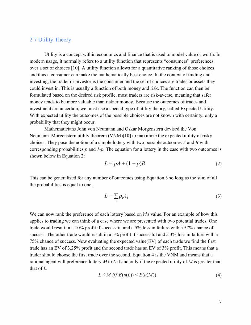
2.7 Utility Theory

Utility is a concept within economics and finance that is used to model value or worth. In modern usage, it normally refers to a utility function that represents “consumers” preferences over a set of choices [10]. A utility function allows for a quantitative ranking of those choices and thus a consumer can make the mathematically best choice. In the context of trading and investing, the trader or investor is the consumer and the set of choices are trades or assets they could invest in. This is usually a function of both money and risk. The function can then be formulated based on the desired risk profile, most traders are risk-averse, meaning that safer money tends to be more valuable than riskier money. Because the outcomes of trades and investment are uncertain, we must use a special type of utility theory, called Expected Utility. With expected utility the outcomes of the possible choices are not known with certainty, only a probability that they might occur.

Mathematicians John von Neumann and Oskar Morgenstern devised the Von Neumann–Morgenstern utility theorem (VNM)[10] to maximize the expected utility of risky choices. They pose the notion of a simple lottery with two possible outcomes A and B with corresponding probabilities p and 1-p. The equation for a lottery in the case with two outcomes is shown below in Equation 2:

A 1 )B L = p + ( − p (2)

This can be generalized for any number of outcomes using Equation 3 so long as the sum of all the probabilities is equal to one.

AL = ∑

ipi i (3)

We can now rank the preference of each lottery based on it’s value. For an example of how this applies to trading we can think of a case where we are presented with two potential trades. One trade would result in a 10% profit if successful and a 5% loss in failure with a 57% chance of success. The other trade would result in a 5% profit if successful and a 3% loss in failure with a 75% chance of success. Now evaluating the expected value(EV) of each trade we find the first trade has an EV of 3.25% profit and the second trade has an EV of 3% profit. This means that a trader should choose the first trade over the second. Equation 4 is the VNM and means that a rational agent will preference lottery M to L if and only if the expected utility of M is greater than that of L.

if f E(u(L)) (u(M )) L ≺ M < E (4)

17

With regards to trading and investing, the VNM gives a user the ability to customize their strategy in a few ways. The first of these ways is that a user can establish a “threshold trades” whereby the EV of any proposed trade must be greater than to be worth it. An example of this geared for longer term investments is to compare a proposed investment against the expected value of a risk-free asset. Another way we can customize this approach is by adding a utility function to adjust the value of our “lotteries” based on our desired risk profile.

3 Literature Review

3.1 Prior Work at WPI

This project is, in many ways, a continuation of previous research conducted at Worcester Polytechnic Institute [11], [12], [13], [14]. The following chapter is a brief summary relevant related research.

3.1.1 Trading Strategies

In Forex Trading System Development (2018) [15] Ziyan Ding devised a “Range And Trend System”. The theory behind the system was to use, Keltner Channels, Triple Exponential Moving Average, and Relative Strength Index, indicators to classify the market as either trending or ranging and trade accordingly. The entry/exit conditions follow the conventional triggers for the indicators, however their exact combination is an invention of the author. The system features built in parameters that can be optimized over time to conform to current market behavior. Monte Carlo simulations of the system show an impressive 32.86% profit, 2.881% maximum drawdown, with 95% confidence.

In Automated Foreign Exchange Trading System (2011)[16] Saraffconn et al, tested four trading strategies based on well known technical indicators. The four strategies were:

➢ Double moving average crossover, which looked for times when moving averages of two different lengths crossed over.

➢ Bollinger Band/ Keltner Channel Counter-Trend, which looked to trade when the price hit support or resistance. For example if the price exceeded the upper Bollinger Band it would sell.

➢ CCI Counter-Trend, this strategy traded on the traditional triggers for the CCI indicating, buying if oversold and selling if overbought.

➢ CCI and Trade Volume Breakout, this strategy tried to detect a price breakout based on the CCI and volume oscillator and ratio indicators.

18

The authors backtested the strategies over the course of one month and found the CCI and Trade Volume Breakout strategy to perform the best. It achieved a profit factor and 3.12 with 72.73% of trades ending profitably.

4 Objective of Research The goal of this Interactive Qualifying Project is to eliminate the psychological and

emotional aspects of manual trading by creating an autonomous trading system which is capable of making short-term trades of foreign currencies. The system will be driven by a combination of scientific and thoughtful technical analysis, and by neural networks. Building on the background information provided in the preceding chapters, this report details several solutions which use neural networks and other artificial intelligence approaches.

There are limitless numbers of algorithmic approaches to trading, however it does not seem possible that a single, realistic algorithm, which would work in all cases, can exist. The goal of this project is therefore to create a set of algorithms that can each function under certain conditions. If time allows, then an overarching system may be created to coordinate these individual algorithms into a single platform which can function under a broader set of circumstances than its constituent systems otherwise would.

5 Methodology

5.1 Setting up a Trading Framework

As a part of our research we wanted to experiment with using neural networks for some of our trading systems. Because of this, we decided we wanted to be able to write our trading systems in Python which has a large library of neural network and machine learning libraries including TensorFlow, Scikit, and Numpy. We also decided that we wanted to use MetaTrader as our broker because of its robust backtesting system which was better than any other broker we looked at. In order to achieve both of these goals we needed to build an interface between MetaTrader and Python.

As a starting point we used a basic system made by Darwinex which had an interface for sending prices between MetaTrader and multiple other languages [17]. This interface was made to only send price information, not to make trades. It made use of the ZeroMQ library, available in multiple languages, to create TCP ports through which the programs could communicate. A server running in MetaTrader would receive requests for data in one TCP port and send replies to those requests in another. A client running in Python could then send requests and read the data received. We decided to expand on this system to fit our needs.

Figure 5.1 shows the final architecture of our interface between Python and MetaTrader. The server, written in MetaTrader, is on the left, and the client, written in Python, is on the right.

19

Connecting them are two TCP ports: a push/pull socket and a push socket. There are two main types of methods available to the client. The first is a push/pull method, such as the tick method which will be discussed later. This type of method sends a message to the push/pull socket and waits until the server sends a response, which the method uses appropriately. The second type is a push method, which again sends a message to the push/pull socket and waits for a response. However, instead of the contents of the message received through the push/pull socket being used, the fact that the message was received is used as a signal that information is available in the push socket which the method pulls and uses.

Figure 5.1: Python/MetaTrader Interface

In order to fulfill the requests from the client, the server checks the the push/pull socket

for messages on a timer of 1 millisecond. When a message is received, the server sends the message to a message handler which makes trades or sends information to the push socket depending on what the request from the client is. Once the message handler has completed the task requested, it returns to the timer method which sends a response to the client.

The most difficult part of creating this system was ensuring that it worked both when testing on the live market and when backtesting using MetaTrader’s built-in backtesting system.

20

This is difficult because the onTimer method does not execute when backtesting is happening. Instead, a method called onTick is run, and once that method finishes running a new tick of historical data is simulated and the onTick method is run again. To get around this, a method called tick was added to the client whose behavior differed on the server depending on whether it was running live or in backtesting mode. When the server is running in backtesting mode it waits for messages requesting data or trades from the client without stopping the onTick method, preventing new ticks from being simulated. Once the client executes the tick method and the tick message is received by the server, the server allows the onTick method to complete, causing a new tick to be simulated. When the server is running on the live market it operates as before, with ticks happening in real time and the tick message not changing that.

The tick method is also used to send information about ticks as they occur. The tick method maintains a backlog of the last 100,000 ticks and the last 10,000 bars which have happened. The tick and bar information is sent by the server through the push/pull socket when a tick message is received. When the server is running in backtesting mode, information about exactly one tick is sent when the tick message is received, as well as information about the previous bar if it was just created by the newest tick. When the server is running live, a list of all ticks and bars which have happened since the last time tick was called is maintained and sent when tick is called. This is necessary because, since the data is coming in real time, any number of ticks may happen between calls to the tick method depending on how fast the client processes.

This method of handling historical data is important for several reasons. First, it allows for the client to run much faster. Instead of the client having to request every piece of data it needs from the server, most of the important data is stored on the client where access is much faster. Even the simplest trading strategies need data from the recent past, but with the amount of data stored by this system, it is very rare than a client will need to manually request any data from the server. Second, there is no good way to request data when the server is backtesting. There are methods which can be used to request data in MetaTrader, but they do not work properly in backtesting mode, meaning this is the only way that clients made to backtest can run. Third, there is no other way for a client to find out how much time has passed when it is running in live mode. If a client requests the current price of a pair twice in a row and receives the same value both times, it has no way of knowing whether the pair changed in value then changed back during the time it took to ask for the current price again or the pair simply has not changed at all. However, with the server tracking and storing every tick, the client can find out exactly what happened since its last call of the tick method with no uncertainty or loss of information. For these reasons, we believe we have developed a robust, but easy to use system for interfacing Python and MetaTrader which could be used by others in the future to research more complex trading strategies in an environment familiar to most coders and with many libraries which are more versatile and of higher quality than those available in the MQL language.

21

5.2 Implementation of Trading Systems

In following with the goal of the project, multiple algorithms were developed in an individual, but coordinated fashion so that they could potentially be combined into a single system at a later date. This section details the development of these approaches.

5.2.1 Approach with Recurrent Neural Networks using Long Short-Term Memory Developed by Thar Min Htet Overview

This trading system is implemented using Recurrent Neural Networks (RNNs) with Long Short-Term Memory (LSTM). The reason for choosing this over other types of neural networks is the ability of RNNs to handle time series data such as financial data very well. LSTM is an add-on to improve the performance of RNN. The details of RNNs and LSTMs will be described in the following section. This model is not designed to trade currencies live, but the purpose of this model is to be incorporated into other trading strategies and support different systems. With further development, such as extending into MetaTrader, this can be used to live trade currencies.

The workflow for the system is summarized as follows: 1. Acquire the currency price data. 2. Preprocess the data. 3. Extract features using Autoencoders. 4. Train the data on LSTM and RNN. 5. Tune Hyperparameters. 6. Test the accuracy with both training and testing data. 7. Make useful prediction on current currency prices.

This flow of events is depicted in the following flowchart, see Figure 5.2. It begins with finding and downloading currency data that will be used during training. Then, as part of preprocessing, the data is denoised using a wavelet transform formula, and transformed using autoencoders, which automatically extracts features. Then the data is divided into training and testing. Next, the training data is fed into the LSTM model, which is fine tuned until the desired accuracy on the training is achieved. If satisfactory, the model is tested on the testing data. At this step, if the model fails to achieve satisfactory accuracy, all the steps starting from feeding the LSTM model is repeated.

22

Figure 5.2: The complete flowchart of training currency data using LSTM

Data and Features

As the saying goes in engineering "Garbage in. Garbage out", one of the most essential parts of a machine learning model is the quality and the relevance of the data. A model is only as good as the data it is fed. The system is trained on an old dataset of EUR/USD. The reason was purely because the transformed data which was processed by a professional was found along with the original data, giving the developer a lot more precision and convenience.

In terms of features, common features such as time, open, high, low, close, and volume are used to train the models. However, more advanced features such as values from indicators such as RSI and MACD can be used for potentially more accurate and relevant predictions.

23

Nonetheless, since such data isn't as widely available as simple price data, automatic features are used instead using the autoencoder. The details behind the autoencoders, however, will not be included since they were found online. Data Preprocessing

Due to the complex nature of currency markets, data is often filled with noise. This might distract the neural network in the learning process of the trends and structure of the price. One solution to this issue is to preprocess the data by removing some of the noise, “cleaning” the data. In this case, a Wavelet Transform is used because it helps preserve the time factor of our data, and an open-sourced implementation of the formula was found:

(a, b) (t)ψ( ) dtXω = 1√a ∫

∞

−∞x a

t−a (5)

where , t represents time and is a continuous function in both the time, b a ∈ R+ ∈ R (t)ψ domain and the frequency domain called the mother wavelet and the overline represents the complex conjugate operation. The preprocessing of data starts by transforming the data using a Wavelet Transform. Then, coefficients that are more than a full standard deviation away from the mean are removed. Then the inverse transform is performed on the data to give the cleaned result. Technology behind the system

RNNs are often proficient in tasks that involve sequences. Since these datasets are time sequences of financial data, an RNN is a logical choice. LSTM is a small, complicated add-on to an RNN in order to prevent technical errors such as exploding and vanishing gradients, which essentially cause the predictor to fail due to the parameters being too small (vanishing) or too big (exploding). Moreover, LSTM has the ability to memorize some value in the past of the sequence because of the memory cells in it, allowing the prediction to relate further into the past of the sequence. Figure 5.4 shows the general structure of an arbitrary LSTM. Figure 5.5 shows a single LSTM cell in details.

Figure 5.3 shows the architecture of a common LSTM model with LSTM as a black box. After the network is trained, the prediction of the sequence works as follows. Firstly, the first value of the input to the sequence (a<0>) is defaulted to 0. Then, the first LSTM cell, takes in the input and multiply with the trained weights, and feeding the outcome to an activation function (softmax, in this case), resulting in the outcome for the first value of the sequence y<1>. y<1> is used as input to next value in the sequence x<2>. And hence, y<t> is always predicted using y<t-1> and the activation value a<t-1> and the pre-trained weights of the network.

Figure 5.4 depicts the inside of a single LSTM cell. In this diagram h<t> is the same as a<t> from Figure 5.3, representing the output value from the cell and also input to the next cell. c<t> is

24

a notation that is used to represent the memory of a cell. The cell takes in c<t-1> which is the current memory of a certain piece of information and decides whether to keep carrying it or not and outputs c<t> to the next cell. Please also be aware of the multiplier and adder units in the figure which correspond to the operations between the outputs from activation functions and c<t-1> to produce c<t> and h<t>.

Figure 5.3: Architecture of Long Short-Term Memory

Figure 5.4: A single cell of an LSTM

In this system, the LSTM model has five layers in total, with three hidden layers. The first layer has 50 neurons, and applies sigmoid activation function. The second and third layers both have 20 neurons each and applies tanh activation function. The fourth layer contains 100 neurons. The last layer contains 1 neuron, which is the output value. These are all implemented using a popular machine learning framework called Keras [18].

To give some background about activation functions, Softmax is an activation function that takes as input a vector of K real numbers, and normalizes it into a probability distribution consisting of K probabilities. Sigmoid produces a value between 0 to 1 or -1 to 1.

25

Tanh a hyperbolic function whose output ranges from -1 to 1. Training the Model

Before training the model, the data is split into the training and testing sets. The model follows a popular convention of an 80/20 ratio of training and testing data. This was accomplished by using popular python libraries for data analysis such as Panda [19] and scikit-learn [20]. The following is the code snippet for splitting the data. X_train, X_test, y_train, y_test =

sklearn.model_selection.train_test_split(X, y, test_size=0.2)

Where X =[Time, Open, High, Low, Volume] , y = [Close], and test_size = 0.2 refers to a 20% test data set size.

The other popular way of splitting data would be train/validation/test. However, for simplicity, only train/test is used. Figure 5.6 shows one method of splitting a dataset.

Figure 5.5: Visualization of splitting datasets [21]

Figure 5.5 also features validation sets. Validation set can be considered as part of training set that is used as test set during training of the model. The advantage of using validation is the prevention of overfitting from hyperparameter tuning. However, this is not implemented in the system for simplicity.

26

5.2.2 Automated Momentum Indication via Candlestick Patterns Developed by Andrew VanOsten

Looking for patterns in candlestick charts is a common practice among traders. Just like any other indicator, these patterns are never perfectly accurate, but they can still provide a valuable indication of trend reversals. These patterns allow the trader to quickly see certain movements of the market through easy to remember shapes. Just as these are relatively easy to read by human eyes, they are very simple to search for with an algorithm. They are defined by the open, high, low, and close prices for each bar—data that are easily available and easy for an algorithm to compare. By using somewhat agreed-upon definitions of common patterns, an algorithm can quickly search an incoming stream of data for potential signals.

These signals each represent the potential for a change in the direction of a trend. However, most traders would not base a trade on this signal alone; similarly, this algorithm takes a slightly deeper approach. A market which is in a downtrend is likely to see several bullish signals as it nears its low point, before reversing and moving upwards. This algorithm looks generates a small positive signal for each bullish signal, and a slightly negative signal for each bearish signal. Different patterns can be given individual weights to allow for differing reliability of each pattern. These small signal values are simply added to an overall momentum “score” which is used as a signal to buy or sell. As time moves forward this score will decrease exponentially, as the signals seen previously will be less accurate as they grow further into the past. The final value of the score at the nth time-step is defined as:

(t ) (t )M n = D · M n−1 + ε (6)

where is the momentum score being generated, is the current time-step, is the(t)M tn tn−1 previous time-step, is the decay constant where , and is the signal beingD 0 < D < 1 ε generated—a constant proportional to the reliability of the pattern that has been observed. This function was created in order to model the desired behavior of the system. When , one(t)M > 1 lot of the selected currency is bought, and when , a lot is sold. When , any(t)M < 1 .5M (t)| | < 0 currently held orders are closed, as this represents a loss of confidence in the indicator. Only one position of one lot may be held at any time.

Disregarding the effects of further input from generated values, adjustment of the ε D value changes the rate at which the value decays. This, in effect, changes how(t)M conservative the algorithm is; a high value makes the program reluctant to close an orderD (putting more trust in the score, at the cost of higher risk), while a low value causes held positions to be closed after a shorter period, limiting risk at the cost of lower potential reward. The weights given to each candlestick pattern can also be tuned to some extent. In general, a pattern of a single bar is given a low weight, while a longer-period pattern of three bars is given more clout.

27

As a compliment to this system, an additional option was added to the program to maximize the profit made per day. As each order was closed, the profit or loss generated by that trade was calculated and logged to a Comma Separated Value (CSV) file, along with the time of day, stored as minutes, beginning at 5:00 PM Eastern Standard Time. This timing convention was used as this is the format used by MetaTrader 4. This logging allowed for instant analysis when a test was completed. When profit/loss was plotted against time of day, one could observe the best times of day during which to trade. This was often quite evident when viewed on a plot. With this information, the system can be instructed to only trade during selects time periods. Because the system relies upon the trends of a market, this layer was quite beneficial to avoid trading during low-volume periods.

5.2.3 Q-Learning using Neural Networks Development by Ben Anderson

This system attempted to use Q-learning along with neural networks to assign values to potential states which the market could have. The first attempt used pure Q-learning. A feed-forward neural network was fed information about the last 20 bars in the market, as well as the current trade, if any, which was in place. In order to make the information about the market more manageable it was rearranged so that all values were relative to the previous bar or other parts of the current bar. The opening price of each bar was represented as the difference between that opening price and the closing price of the previous bar, the high was represented as the difference between the high and the open, the low was represented as the difference between the low and the close, and the close was represented as the difference between the open and the close. Representing these values in this way allowed the system to consider each state independently without having to account for differences in the range of input data. Once all data was fed in, the network was trained using equation 4.

oss Q(s ) (s ))| l = | t − (rt + γ · Q t+1 (7)

In this formula Q(s) is used to represent the predicted reward of a certain state, r is the received reward, and ɣ was the decay factor which was set to 0.9. The neural network was trained to minimize this loss function for 5 million iterations.

A slightly different approach of using Q-learning was used to make a second neural network. This design came from the realization that in order to go from making a prediction about the future behavior of the market to predicting a reward, the neural network had to do a multiplication of the current amount traded and the predicted change in the market. This is possible, but unnecessarily complicated when it is known that the multiplication is necessary. In light of this fact, a second neural network was designed where it was always assumed that one lot would be bought. The value of a state could be calculated by multiplying the actual trade size by the value of the state where one lot was owned. The same formula was used to calculate loss for

28

this network, but r was replaced with the change of the next bar. This network was trained for 10 million iterations.

5.2.4 Using Expected Utility Theory for Asset Allocation Development by Nick Nugent

As covered in Section 2.7 the Von Neumann–Morgenstern (VNM) utility theorem can be used to rank the value of choices, and so we decided to try to use it to combine our individual trading strategies into one system.

First, let us look at the simplest case of this application. Suppose we have a number of algorithms that propose n number of trades at the same time. Each trade has a known take profit and stop loss, and the historical win rate of the algorithm is known. From there, the expected utility of each trade can be evaluated and the trades ranked using Equation 2. Then we can discard any trades with a negative expected utility and size the trading according to the ranking where the top ranked trade is the largest.

We conducted a proof of conduct on this concept to verify it could work. We made a mock up system of “algorithms.” These algorithms merely generated trades with random take profits, stop loses, and probabilities of success. For the test shown in Figure 5.6 the profit and loss was determined randomly based on a Gaussian distribution with a mean of 2% and standard deviation of .3% and the probability of success with a Gaussian distribution with a mean of 50% and a standard deviation of 12%. Those trades were then executed twice, once using a naive allocation and once using a expected utility based allocation. For the naive allocation the starting balance, $1000, was split evenly between the three algorithms and they traded independently. Using that approach we see a small profit over 50 trades. For the expected utility based allocation at each step the three possible trades have their expected utility calculated, they are then ranked and allocated a portion of the account balance based on their rank. If the trade has a negative expected utility the money allocated to it is held rather than traded. The result was that the expected utility based allocation performed much better than the naive allocation.

29

Figure 5.6: Testing Naive vs Expected Utility Allocation.

Even though we have shown that an expected utility based allocation is better than a

naive one there are a number of problems with implementing this in our system. The first of which is that unless there was a large enough system of algorithms, simultaneous trade proposals are unlikely to occur, which would nullify the lot sizing aspect of the system. The system would, however, still be of some use. It would act as a filter to block trades with a negative expected utility and thus still increase the performance of the system. The other major problem with implementing this is that it relies on trades with a defined outcome, meaning they must have a take profit and stop loss. For many algorithms, including the ones researched in this report, that is not practical as they have more complex exit conditions.

Because we could not implement expected utility based allocation at a trade-by-trade level we decided to take a step back and look at it as a portfolio investing problem. We essentially have a number of competing assets, the assets being the algorithms, that we want to invest some percentage of our account balance in to maximize our profit. Because we do not have defined outcomes using this method we must modify our utility function so that it can work with historical performance data. There are many utility functions concerning portfolio allocation for a risk averse investor and we will use a simpler one that considers the expected return and volatility.

(r) .5 U = E − 0 * A * σ2 (8)

Here E(r) is the expected return of the asset which would be determined from the historical returns. A is a risk aversion coefficient from 1 to 5 with 5 being most risk averse. σ is the volatility of the asset, again determined from historical data.

The utility scores of every algorithm would again be ranked and compared to a cut-off value such as a risk-free U.S. Treasury bond to determine if it should be rejected and how much

30

should be invested. Using this method we would periodically reallocate based on the updated performance metrics of the algorithms.

31

6 Results

6.1 Approach with Recurrent Neural Networks using Long Short-Term Memory Since the system was implemented to predict numbers, i.e, future prices, the problem

falls under regression, instead of classification. Therefore, the most popular way to evaluate the performance of a regression predictor is to generate charts to compare the values between predictions and training/testing data. Due to the restriction of time and convenience, the system is trained on the old data before 2008. However, the system itself is timeless and should perform in similar way when the most current data is fed to train the system. In Figure 6.1 graphs are generated that highlight the performance of the system. To show the comparison more vividly, both graphs for logarithmic return and market price are generated.

Figure 6.1: Overall comparison between predicted price and actual price In the comparison from Figure 6.1, although there are some big spikes of noise for the log

return, the prediction for market price seems to work pretty well, even overshadowing the actual price. Therefore, to make it clearer, graphs for smaller time duration are generated, as seen in Figure 6.2.

In Figure 6.2 we can observe that the prediction fits fairly well with the actual data in general, except around time stamp 48, which shows a massive gap between the two. This could be caused by the regularization that was done to prevent the model from overfitting the data.

32

Figure 6.2: Comparison of the first 50 testing examples

Similar to the previous graph from Figure 6.2, in Figure 6.3 the model does a pretty good

job fitting the prediction line. The big error at the very start is a continuity from the previous graph, and is likely to be caused by the same reason.

Figure 6.3: Comparison of the second 50 examples

33

In Figures 6.4 and 6.5, the model performs pretty well at the end of the dataset. However, the prediction for log return (upper subplot in both Figures) seems to be very flat in comparison to the actual data, which has some noise. But because the value from the market price can be used as standalone data in a live trading system, the relatively poor performance of the log system does not matter that much in our case.

As for further concerns, the model seems to be fitting too well, and there is a risk of overfitting. This can be resolved by incrementing the L2 regularization factors and dropout weights, in the machine learning techniques used in this model to prevent overfitting.

Figure 6.4: Comparison of the second to last 50 examples

34

Figure 6.5: Comparison of the last 62 examples

6.2 Automated Momentum Indication via Candlestick Patterns As described in Section 5.2.2, a system was implemented using Python and linked to

MetaTrader 4 via the interface described in Section 5.1. A variety of single and triple candlestick patterns were experimented with. Table 6.1 below describes the patterns and associated weights which were used via trial and error. Note that the Hammer and Shooting Star patterns are equivalent, but bullish and bearish respectively. The same is true for the Morning Star and Evening Star patterns. This is reflected in the opposite values associated with each. For the sake of comparison, GBPUSD 5 minute data was used for this section. Other currency pairs and timeframes could be used, but would likely require different tuning of values.ε

Table 6.1: Chart Patterns Used and Associated Weights

Candlestick Pattern Name Associated valuesε

Hammer 0.3

35

Shooting Star -0.3

Morning Star 0.8

Evening Star -0.8

To complete the implementation of the equation described in Section 5.2.2, a decay value of was settled on for the final form of the system. In a slight addition to the theory.9D = 0 layed out in the previous chapter, one additional condition was added to the flow of the program. If the bar being examined at a given time step is a Doji, which I have defined as a candlestick with open and close prices which are within 0.5 pips of each other, then the value was(t)M multiplied by 0.25. This condition was added because a Doji symbolizes indecision on the part of traders in the given market. Accelerated decay of the momentum value at these points improves the system’s model by accounting for this indecision.

With these conditions in place, the following results were generated. Figure 6.6 shows the balance of an account which was controlled by the system from 3/1/2019 to 3/31/2019. The system ran on GBPUSD 5 minute data, and began with an account balance of $10,000 USD. After one month, the balance was $9,574 USD—a return of -4.26%.

Figure 6.6: GBPUSD-M5 account balance over one month with no time of day restriction

In order to improve performance, the system allows for easy analysis of individual trade profits based on the time of day of the trade. The profit made from each trade in the previously described trial was logged to a CSV file, then plotted vs the time of day represented as minutes since 5:00 PM Eastern Standard Time (EST). The result is shown in Figure 6.7. Each point in the

36

graph represents a single trade. The horizontal axis represents time in minutes since the simulation started (in this case, 3/1/2019).

Figure 6.7: GBPUSD-M5 trade profit vs time of day over one month of trading

This figure is not very useful for determining the most profitable times of day to trade, but it does show that the magnitude of the profit appears to be greater in the second half of the day (minutes 720-1440). To determine the best way to take advantage of this, the same data can be represented in a different way. Figure 6.8 shows the average profit from trades for various times of day. In this graph, it can clearly be seen that trades in the second half of the time period tend to provide a significantly more positive outcome. These hours, 12 through 24 in the figure, correspond to 5:00 AM to 5:00 PM EST, accounting for most of the London trading session and the entirety of the New York session. This is a logical time for volatility to be relatively high, and for the market to be trending—helpful factors for this system.

37

Figure 6.8: GBPUSD-M5 average trade profit vs time of day over one month of trading

The preceding figure provides information that allows the system to be further tuned. One can simply disallow the system from trading during hours 0-12. With this change in place, the account balance for the same time period is shown in Figure 6.9. As shown, the system’s account finished the month with $9179 USD, or a return of -8.21%.

Figure 6.9: GBPUSD-M5 account balance over one month with time of day restriction

38

In both Figures 6.6 and 6.9, many of the losses seem to happen as large jumps in the graphs, i.e. a handful of highly negative trades. One approach to solving this problem is through the use of a stop-loss. This will cut off any damaging trades before they become major losses. Figure 6.10 displays the results of the system, again on the same dataset, with a stop-loss set at $100 USD (e.g. a trade will automatically close when a loss reaches $100 USD). This trial did not use the time of day restriction.

Figure 6.10: GBPUSD-M5 account balance over one month with stop-loss

6.3 Q-Learning using Neural Networks

To test Q-learning using a Feed Forward Network (FFN), the system was allowed to run for 1000 simulated minutes, and allowed to make a trade every bar. No commission or spread was taken into account. For each simulated bar, the system evaluated how many lots it thought was the optimal amount to own. It was then allowed to trade until it had that amount. This was done multiple times on multiple independently trained networks.

The following is the result of a trial. The result of this trial is very similar to the results of all other trials. In total, the agent lost $430. It chose to own one lot 58% of the time, own -1 lots 23% of the time, and chose to own either -0.5, 0, or 0.5 lots the rest of the time. Figure 6.11 shows how little the system was able to predict. The change in the market during the next bar and the predicted value of owning 1 lot are not related ( ). Figure 6.12 helps explain.003R2 = 0 why this problem occurs. If the market is going to go up, buying should be desirable and selling should not be. If the market is going to go down the opposite should be true. However, the system finds that the more desirable owning 1 lot is, the more desirable owning -1 lots is (

39

). This is a contradiction which prevents this system from being able to make.6357R2 = 0 accurate predictions.

Figure 6.11: Prediction vs change for Q-Learning

Figure 6.12: Desirability of owning 1 vs -1 lots

40

Positive-only Q-learning was also run in trials of 1000 bars on several sets of data with

multiple independently trained networks. The following is a typical result. In Figure 6.13, it can be seen that there is again no relation between desirability of a state and how much the market changed during the next tick: . If the product between the predicted value and the.0008R2 = 0 actual market change is taken for each bar and summed, it can be found that this algorithm does not make money. In this particular case, the result of this calculation is -0.558. The magnitude of this value does not have any innate meaning, but it can be calculated that in this trial the algorithm performing randomly would have gotten a value of -0.642. The similarity in these values shows that the algorithm did only slightly better than random, and not well enough to make a profit.

Figure 6.13: Prediction vs change for positive Q-Learning

41

7 Conclusions and Further Work In this project, we aimed to create new systems which were individually capable of

performing short-term trading of currency pairs with the goal of making a profit. Through automated technical analysis and machine learning, three systems were created which can examine past data and make trades accordingly. As part of this, a system was developed to allow MetaTrader 4 and its MQL4 language to communicate with Python scripts. This allowed for the use of common Python libraries, broadening the potential of the project, and opening the doors to machine learning techniques.

Many of the results that have been displayed in the preceding chapter are not terribly positive. However, this makes them no less valuable—they provide a basis on which further work can be performed. Additionally, we do not believe that our approaches have been entirely invalidated. The systems and associated ideas that have been presented in this report could potentially be expanded upon in order to develop a more profitable system which revolves around similar core principles. Though the systems were not profitable, we still believe that we have accomplished our goal—we created three systems of our own design and developed them as best we could within the timeframe of the project.

Ideally we would have been able to test the utility theory based allocation method, however the lack of profitable algorithms makes its implementation within this system moot. We would like to see it tested with profitable algorithms and improved on. Better utility functions could be defined that would improve profit while managing risk. We would also like to see an improved system for the allocation weights, which is the amount of money given to each algorithm. In the system described in this report the allocations are fixed based on the utility rank, but this could be improved by using something like reinforcement learning to size the allocations.

42

References [1] Alain Chaboud, Benjamin Chiquoine, Erik Hjalmarsson, Clara Vega, Rise of the

Machines: Algorithmic Trading in the Foreign Exchange Market. International Finance Discussion Papers, Board of Governors of the Federal Reserve System, 2009. https://www.federalreserve.gov/pubs/ifdp/2009/980/ifdp980.pdf

[2] Kanika Khera, Inderpal Singh, Effect of Macro Economic Factors On Rupee Value. Delhi Business Review, Vol. 16, No. 1, 2015. http://www.delhibusinessreview.org/V16n1/dbr_v16n1h.pdf

[3] Edward W. Sun, Omid Rezania, Svetlozar T. Rachev, Frank J. Fabozzi, Analysis of the Intraday Effects of Economic Releases on the Currency Market. Journal of International Money and Finance, Vol. 30, Issue 4, June 2011. https://www.sciencedirect.com/science/article/pii/S0261560611000441

[4] Karl B. Diether, Kuan-Hui Lee, Ingrid M. Werner, Short-Sale Strategies and Return Predictability. The Review of Financial Studies, Vol. 22, Issue 2, Feb. 2009. https://academic.oup.com/rfs/article/22/2/575/1596032

[5] Moorad Choudhry, An Introduction to Bond Markets, John Wiley and Sons, 2010. https://ebookcentral-proquest-com.ezproxy.wpi.edu/lib/wpi/detail.action?docID=624740

[6] F. Lhabitant, Commodity Trading Strategies: Examples of Trading Rules and Signals from the CTA Sector, John Wiley and Sons, 2008. https://learning.oreilly.com/library/view/the-handbook-of/9780470117644/10_chap01.html

[7] Ronald C. Spurga, Commodity Fundamentals: How to Trade the Precious Metals, Energy, Grain, and Tropical Commodity Markets, John Wiley and Sons, 2006. https://learning.oreilly.com/library/view/commodity-fundamentals-how/9780471788515/

[8] Michael D. Archer, Getting Started in Currency Trading, John Wiley and Sons, 2012. https://learning.oreilly.com/library/view/getting-started-in/9781118281987/OEBPS/9781118281987_epub_ch_01.htm

[9] Kathy Lien, Day Trading and Swing Trading the Currency Market Technical and Fundamental Strategies to Profit From Market Moves, John Wiley and Sons, 2016. https://ebookcentral-proquest-com.ezproxy.wpi.edu/lib/wpi/detail.action?docID=4187281

43

[10] Von Neumann, J. and Morgenstern, O. (2007). Theory of games and economic behavior. Princeton, NJ: Princeton Univ. Pr.

[11] Zhang, N. and Zhou, Z. (2016). Trading System Development. [online] WPI. Available at: https://digitalcommons.wpi.edu/iqp-all/1908/ [Accessed Apr. 2019].

[12] Allen, J., Chen, L. and Antontas, S. (2018). Trading System Development IQP 17_18. [online] WPI. Available at: https://digitalcommons.wpi.edu/iqp-all/5190/ [Accessed Apr. 2019].

[13] Diniz, B., O'Day, B. and Stimson, D. (2015). Trading System Development. [online] WPI. Available at: https://digitalcommons.wpi.edu/iqp-all/1977/ [Accessed Apr. 2019].

[14] Nottage, J. (2014). Stock Trading Systems: Analysis and Development of a System of Systems. [online] WPI. Available at: https://digitalcommons.wpi.edu/iqp-all/1446/ [Accessed 23 Apr. 2019].

[15] M. Ma, “Forex Trading System Development,” ECE, WPI, IQP, Jan 2018.[Online]. Available: https://digitalcommons.wpi.edu/iqp-all/2281/ [Accessed Apr. 2019]

[16] Sarafconn, D., Mehta, J. and Menghini, M. (2011). Automated Foreign Exchange Trading System. [online] WPI. Available at: https://digitalcommons.wpi.edu/iqp-all/3292/ [Accessed Apr. 2019].

[17] Darwinex, ZeroMQ – How To Interface Python/R with MetaTrader, Aug. 2017, https://blog.darwinex.com/zeromq-interface-python-r-metatrader4/

[18] Keras, an open-source neural network library written in Python. https://keras.io

[19] Pandas, a Python library used for data processing. https://pandas.pydata.org

[20] SciKit Learn, a Python library used for data processing. https://scikit-learn.org/stable/

[21] Adi Bronshtein, Train/Test Split and Cross Validation in Python, Towards Data Science, May 17, 2017. https://towardsdatascience.com/train-test-split-and-cross-validation-in-python-80b61beca4b6

44

Appendices

Appendix A: MQL4 Code to Interface With Python The following code is for the server which can interface with the Python code shown later. Two tcp ports are made (localhost:5555 and localhost:5556) and can be connected to by a client. The architecture of this program is described in section 5.1. // Required: MQL-ZMQ from https://github.com/dingmaotu/mql-zmq #include <Zmq/Zmq.mqh> extern string ZEROMQ_PROTOCOL = "tcp"; extern string HOSTNAME = "*"; extern int REP_PORT = 5555; extern int PUSH_PORT = 5556; extern int MILLISECOND_TIMER = 1; // 1 millisecond // CREATE ZeroMQ Context Context context(PROJECT_NAME); // CREATE ZMQ_REP SOCKET Socket repSocket(context,ZMQ_REP); // CREATE ZMQ_PUSH SOCKET Socket pushSocket(context,ZMQ_PUSH); // VARIABLES FOR LATER int debug = 0; uchar data[]; ZmqMsg request; string tickdata = "TICK"; //+------------------------------------------------------------------+ //| Expert initialization function | //+------------------------------------------------------------------+ int OnInit() { //--- EventSetMillisecondTimer(MILLISECOND_TIMER); // Set Millisecond Timer to get client socket input Print("[REP] Binding MT4 Server to Socket on Port " + REP_PORT + ".."); Print("[PUSH] Binding MT4 Server to Socket on Port " + PUSH_PORT + "..");

45

repSocket.bind(StringFormat("%s://%s:%d", ZEROMQ_PROTOCOL, HOSTNAME, REP_PORT)); pushSocket.bind(StringFormat("%s://%s:%d", ZEROMQ_PROTOCOL, HOSTNAME, PUSH_PORT)); /* Maximum amount of time in milliseconds that the thread will try to send messages after its socket has been closed (the default value of -1 means to linger forever): */ repSocket.setLinger(1000); // 1000 milliseconds /* If we initiate socket.send() without having a corresponding socket draining the queue, we'll eat up memory as the socket just keeps enqueueing messages. So how many messages do we want ZeroMQ to buffer in RAM before blocking the socket? */ repSocket.setSendHighWaterMark(5); // 5 messages only. //--- return(INIT_SUCCEEDED); } //+------------------------------------------------------------------+ //| Expert deinitialization function | //+------------------------------------------------------------------+ void OnDeinit(const int reason) { //--- uint timer = GetTickCount(); //Wait for one second to inform client of closing repSocket.recv(request, true); while (GetTickCount() - timer < 1000 && request.size() <= 0) repSocket.recv(request, true); if (request.size() <= 0) repSocket.send("STOP", true); if (debug) { Print("Stopping"); ArrayResize(data, request.size()); request.getData(data);

46

string dataStr = CharArrayToString(data); Print(dataStr); } Print("[REP] Unbinding MT4 Server from Socket on Port " + REP_PORT + ".."); repSocket.unbind(StringFormat("%s://%s:%d", ZEROMQ_PROTOCOL, HOSTNAME, REP_PORT)); Print("[PUSH] Unbinding MT4 Server from Socket on Port " + PUSH_PORT + ".."); pushSocket.unbind(StringFormat("%s://%s:%d", ZEROMQ_PROTOCOL, HOSTNAME, PUSH_PORT)); } //+------------------------------------------------------------------+ //| Expert timer function | //+------------------------------------------------------------------+ void OnTimer() { //--- /* For this example, we need: 1) socket.recv(request,true) 2) MessageHandler() to process the request 3) socket.send(reply) */ // Get client's response, but don't wait. repSocket.recv(request,true); // MessageHandler() should go here. string reply = MessageHandler(request); if (reply != "") { // socket.send(reply) should go here. ZmqMsg msg(reply); repSocket.send(msg); } } void OnTick() { string send = ""; if (IsTesting()) {

47

bool done = False; while (!done && !IsStopped()) { repSocket.recv(request, true); string reply = MessageHandler(request); if (reply == "TICK") { done = True; } else if (reply != "") { if (debug) { Print(reply); } ZmqMsg msg(reply); repSocket.send(msg); } } //Send tick info to Python send = StringFormat("TICK|%f|%f", Bid, Ask); if (Volume[0] == 1) { StringAdd(send, StringFormat("|BAR|%f|%f|%f|%f", High[1], Low[1], Open[1], Close[1])); } if (debug) Print(send); repSocket.send(send); } else { if (StringLen(tickdata) < 10000) { StringAdd(tickdata, StringFormat("|%f|%f", Bid, Ask)); if (Volume[0] == 1) { StringAdd(tickdata, StringFormat("|BAR|%f|%f|%f|%f|TICK", High[1], Low[1], Open[1], Close[1])); } } } } //+------------------------------------------------------------------+ string MessageHandler(ZmqMsg &request) { // Output object

48

string reply = ""; // Message components for later. string components[]; if(request.size() > 0) { // Get data from request ArrayResize(data, request.size()); request.getData(data); string dataStr = CharArrayToString(data); if (debug) { Print(dataStr); } // Process data ParseZmqMessage(dataStr, components); // Interpret data reply = InterpretZmqMessage(&pushSocket, components); } else { // NO DATA RECEIVED } return(reply); } // Interpret Zmq Message and perform actions string InterpretZmqMessage(Socket &pSocket, string& compArray[]) { //Print("ZMQ: Interpreting Message.."); int switch_action = 0; if(compArray[0] == "TRADE" && compArray[1] == "OPEN") switch_action = 1; if(compArray[0] == "RATES") switch_action = 2; if(compArray[0] == "TRADE" && compArray[1] == "CLOSE") switch_action = 3; if(compArray[0] == "DATA") switch_action = 4; if(compArray[0] == "TICK") switch_action = 5; if(compArray[0] == "TIME") switch_action = 6;

49

string ret = ""; int ticket = -1; bool ans = FALSE; double price_array[]; ArraySetAsSeries(price_array, true); double price; int price_count = 0; switch(switch_action) { case 1: if (compArray[3] == "CURRENT") compArray[3] = NULL; SymbolSelect(compArray[3], true); price = MarketInfo(compArray[3], (StringToInteger(compArray[3])?MODE_BID:MODE_ASK)); price = (StringToDouble(compArray[4])?compArray[4]:price); ticket = OrderSend(compArray[3], compArray[2], compArray[7], price, 3, compArray[5], compArray[6], compArray[8], 0, 0, Green); if (ticket <= 0) { Print("Order Open Error: ", GetLastError()); } InformPullClient(pSocket, StringFormat("TICKET|%d", ticket)); break; case 2: ret = "N/A"; if(ArraySize(compArray) > 1) { if (compArray[1] == "CURRENT") compArray[1] = NULL; ret = GetBidAsk(compArray[1]); } InformPullClient(pSocket, ret); break; case 3: if (OrderSelect(compArray[2], SELECT_BY_TICKET)) { if (OrderType() >= 2) ans = OrderDelete(compArray[2]); else ans = OrderClose(compArray[2], OrderLots(), MarketInfo(OrderSymbol(), (OrderType()?MODE_BID:MODE_ASK)), 3, Red); } ret = StringFormat("CLOSE|%s|%s", compArray[2], (ans?"True":"False")); if (!ans) { Print("Order Close Error: ", GetLastError());

50

} InformPullClient(pSocket, ret); break; case 4: InformPullClient(pSocket, "HISTORICAL DATA Instruction Received"); // Format: DATA|SYMBOL|TIMEFRAME|START_DATETIME|END_DATETIME price_count = CopyClose(compArray[1], StrToInteger(compArray[2]), StrToTime(compArray[3]), StrToTime(compArray[4]), price_array); if (price_count > 0) { ret = ""; // Construct string of price|price|price|.. etc and send to PULL client. for(int i = 0; i < price_count; i++ ) { if(i == 0) ret = compArray[1] + "|" + DoubleToStr(price_array[i], 5); else if(i > 0) { ret = ret + "|" + DoubleToStr(price_array[i], 5); } } if (debug) { Print("Sending: " + ret); } // Send data to PULL client. InformPullClient(pSocket, StringFormat("%s", ret)); // ret = ""; } break; case 5: if (IsTesting()) return "TICK"; ret = tickdata; tickdata = "TICK"; return ret; break;

51

case 6: { datetime now_dt = TimeCurrent(); MqlDateTime now; TimeToStruct(now_dt,now); InformPullClient(pSocket, StringFormat("TIME|%d|%d|%d",now.day_of_week,now.hour,now.min)); break; } default: break; } return "[SERVER] Processing Request"; } // Parse Zmq Message void ParseZmqMessage(string& message, string& retArray[]) { //Print("Parsing: " + message); string sep = "|"; ushort u_sep = StringGetCharacter(sep,0); int splits = StringSplit(message, u_sep, retArray); } //+------------------------------------------------------------------+ // Generate string for Bid/Ask by symbol string GetBidAsk(string symbol) { symbol = symbol; double bid = MarketInfo(symbol, MODE_BID); double ask = MarketInfo(symbol, MODE_ASK); return(StringFormat("%f|%f", bid, ask)); } // Inform Client void InformPullClient(Socket& pushSocket, string message) { if (debug) { Print(message); } ZmqMsg pushReply(StringFormat("%s", message)); // pushSocket.send(pushReply,true,false);

52

pushSocket.send(pushReply,true); // NON-BLOCKING // pushSocket.send(pushReply,false); // BLOCKING }

Appendix B: Python Code to Interface With MetaTrader 4 This code is a Python client made to interact with the server above. It contains several methods which allow for easy interfacing with the server, as well as automatic storing of recent data as described in section 5.1. # IMPORT zmq library import zmq import re #Create constants OP_BUY = 0 OP_SELL = 1 OP_BUYLIMIT = 2 OP_SELLLIMIT = 3 OP_BUYSTOP = 4 OP_SELLSTOP = 5 #Timeframe constants M1 = "1" M5 = "5" M15 = "15" M30 = "30" H1 = "60" H4 = "240" D1 = "1440" W1 = "10080" # Keep track of all Bid and Ask data gathered from tick() Bids = [] Asks = [] Bars = [] # Create ZMQ Context context = zmq.Context() # Create REQ Socket reqSocket = context.socket(zmq.REQ) reqSocket.connect("tcp://localhost:5555") # Create PULL Socket

53

pullSocket = context.socket(zmq.PULL) pullSocket.connect("tcp://localhost:5556") #Advances backtesting by 1 tick if backtesting #Collects all tick data since last call if live trading #Returns True if updated, else False #Stores bid and ask in Bids and Asks #If a new bar was formed, the previous one is stored in Bars def tick(): global Asks, Bids, Bars msg = remote_send(reqSocket, b'TICK') values = msg.split('|') # Live trading and tick has not yet happened if values == ['TICK'] or values == ['']: return False mode = 't' i = 0 while i < len(values): if values[i] == 'TICK': mode = 't' i += 1 elif values[i] == 'BAR': mode = 'b' i+= 1 else: if mode == 't': Bids.insert(0, float(values[i])) Asks.insert(0, float(values[i+1])) i += 2 elif mode == 'b': Bars.insert(0, Bar(float(values[i]), float(values[i+1]), float(values[i+2]), float(values[i+3]))) i += 4 if len(Asks) > 110000: Asks = Asks[:100000] Bids = Bids[:100000] if len(Bars) > 15000: Bars = Bars[:10000] return True #Input symbol as string #Output (Ask, Bid)

54

def rates(symbol = 'CURRENT'): template = b'RATES|%s' remote_send(reqSocket, template%(bytes(symbol, 'utf-8'))) msg = remote_pull(pullSocket) match = re.match(r'b\'([\d\.]*)\|([\d\.]*)\'', str(msg)) if match == None: return 0, 0 return float(match.group(1)), float(match.group(2)) #Returns the ticket number, or -1 if unsuccessful #tradeType is one of the OP's defined at the top def openTrade(tradeType, symbol = 'CURRENT', vol = 1, price = 0, sl = 0, tp = 0, comment = "Py-to-MT"): template = b'TRADE|OPEN|%d|%s|%f|%f|%f|%f|%s' remote_send(reqSocket, template%(tradeType, bytes(symbol, 'utf-8'), price, sl, tp, vol, bytes(comment, 'utf-8'))) msg = remote_pull(pullSocket) match = re.match(r'b\'TICKET\|([-\d]*)\'', str(msg)) if match == None: return -1 return int(match.group(1)) #returns True if succeeded, else False def closeTrade(ticket): template = b'TRADE|CLOSE|%d' remote_send(reqSocket, template%(ticket)) msg = remote_pull(pullSocket) match = re.match(r'b\'CLOSE\|[\d]*\|(True|False)\'', str(msg)) if match == None: return False return match.group(1) == 'True' # returns an array of the data requested # dates are formatted as "yyyy.mm.dd hh.mm" i.e. "2018.01.31 8:30" # if it catches the exception, you're probably asking for data that it doesn't have # or it can't understand the parameters you're giving it #Ex: getData("EURUSD", H1, "2019.01.23 00:00", "2019.01.24 00:00") def getData(pair, timeframe, start_date, end_date): try: request = bytes("DATA|" + pair + "-5|" + timeframe + "|" + start_date + "|" + end_date, "utf-8")

55

remote_send(reqSocket,request) remote_pull(pullSocket) # gather confirmation message incoming = remote_pull(pullSocket).decode("utf-8").split("|") # gather incoming data del incoming[0] data = [] for dat in incoming: data.append(float(dat)) return data except zmq.Again as e: print("Error (likely bad parameters)") raise(e) # Gets the current day of the week, hour, and minute from MT4 # Returns a WeekTime object def getTime(): request = b'TIME' remote_send(reqSocket, request) try: msg = remote_pull(pullSocket).decode("utf-8").split("|") wTime = WeekTime(int(msg[1]), int(msg[2]), int(msg[3])) return wTime except zmq.Again as e: print("error") raise(e) # Function to send commands to ZeroMQ MT4 EA def remote_send(socket, data): try: socket.send(data) msg = socket.recv_string() if msg == "STOP": raise Exception("Server has been terminated") return msg except zmq.Again as e: print("Error: Major Error") raise(e) # Function to retrieve data from ZeroMQ MT4 EA def remote_pull(socket): try: msg = socket.recv() return msg

56

except zmq.Again as e: print("Error: Major Error") raise(e) class Bar: #Represents a bar on the chart def __init__(self, High, Low, Open, Close): self.High = High self.Low = Low self.Open = Open self.Close = Close # Stores day of week, hour, and minute for logging trades class WeekTime: def __init__(self, DayOfWeek, Hour, Minute): self.DayOfWeek = DayOfWeek self.Hour = Hour self.Minute = Minute def minsSinceMidnight(self): return self.Hour*60 + self.Minute

Appendix C: Code for Approach with Recurrent Neural Networks using Long Short-Term Memory

encoded_model.py

import tensorflow as tf from keras.models import Model import keras.layers as kl import keras as kr from sklearn.metrics import r2_score, mean_squared_error import pandas as pd import numpy as np import matplotlib.pyplot as plt def model(epochs, regularizer1, regularizer2): train_data = np.array(pd.read_csv( "data/encoded_return_train_data.csv", index_col=0)) train_data = np.reshape(train_data, (len(train_data), 20)) train_y = np.array(pd.read_csv("data/log_train_y.csv", index_col=0)) test_y = np.array(pd.read_csv("data/log_test_y.csv", index_col=0)) test_data = np.array(pd.read_csv( "data/encoded_return_test_data.csv", index_col=0)) test_data = np.reshape(test_data, (len(test_data), 20))

57

price = np.array(pd.read_csv("data/test_price.csv", index_col=0)) ''' The following commented code corresponds to building the model and training it. ''' # model = kr.models.Sequential() # model.add(kl.Dense(50, activation="sigmoid", activity_regularizer=kr.regularizers.l2(0))) # model.add(kl.Dense(20, input_dim=20, activation="tanh", activity_regularizer=kr.regularizers.l2(regularizer1))) # model.add(kl.Dense(20, activation="tanh", activity_regularizer=kr.regularizers.l2(regularizer2))) # model.add(kl.Dense(100)) # model.add(kl.Dense(1)) # model.fit(train_data, train_y, epochs=epochs) # model.save("models/trained_model.h5") ''' Loading the previously trained model ''' model = kr.models.load_model("models/trained_model.h5") model.compile(optimizer="sgd", loss="mean_squared_error") predicted_data = [] predicted_price = [] for i in range(len(test_data)): prediction = model.predict(np.reshape(test_data[i], (1, 20))) predicted_data.append(prediction) price_pred = np.exp(prediction)*price[i] predicted_price.append(price_pred) #saving the predictions to csv file pd.DataFrame(np.reshape(predicted_price, (len(predicted_price, )))).to_csv( "data/predicted_price.csv") pd.DataFrame(price).to_csv("data/price.csv") #generation of graphs plt.figure(1) plt.subplot(2, 1, 1) plt.plot(np.arange(len(predicted_data[2750:2800])), np.reshape(test_y[2750:2800,:], (len(test_y[2750:2800,:]))), np.reshape(predicted_data[2750:2800], (len(predicted_data[2750:2800])))) plt.title("Prediction vs Actual") plt.ylabel("Log Return") plt.legend(["Actual", "Prediction"])

58

plt.subplot(2, 1, 2) plt.plot(np.arange(len(predicted_price[2750:2800])), np.reshape(price[2750:2800,:], (len(price[2750:2800,:]))), np.reshape(predicted_price[2750:2800], (len(predicted_price[2750:2800])))) plt.xlabel("Time stamp") plt.ylabel("Market Price") plt.legend(["Actual", "Prediction"]) plt.show() price_r_score = r2_score(np.reshape( predicted_price, (len(predicted_price))), price) return_r_score = r2_score(np.reshape( predicted_data, (len(predicted_data))), test_y) price_mse = mean_squared_error(np.reshape( predicted_price, (len(predicted_price))), price) return_mse = mean_squared_error(np.reshape( predicted_data, (len(predicted_data))), test_y) dataset = [] values = np.array([regularizer1, regularizer2, epochs, price_r_score, return_r_score, price_mse, return_mse]) dataset.append(values) dataset = pd.DataFrame(dataset, columns=[ "regularizer1", "regularizer2", "epochs", "price_r_score", "return_r_score", "price_mse", "return_mse"]) return dataset if __name__ == "__main__": dataset = model(500, 0.05, 0.01) # Epochs 500

preprocess.py

import numpy as np import pandas as pd import pywt class PreProcess: def __init__(self, split, feature_split): self.split = split self.feature_split = feature_split self.stock_data = pd.read_csv("eurusd_data.csv") # generate wavelet transform data

59

def generate_wavelet_train(self): train_data = [] test_data = [] log_train_data = [] for i in range((len(self.stock_data)//10)*10 - 11): train = [] log_ret = [] for j in range(1, 6): x = np.array(self.stock_data.iloc[i: i + 11, j]) (ca, cd) = pywt.dwt(x, "haar") cat = pywt.threshold(ca, np.std(ca), mode="soft") cdt = pywt.threshold(cd, np.std(cd), mode="soft") tx = pywt.idwt(cat, cdt, "haar") log = np.diff(np.log(tx))*100 macd = np.mean(x[5:]) - np.mean(x) sd = np.std(x) log_ret = np.append(log_ret, log) x_tech = np.append(macd*10, sd) train = np.append(train, x_tech) train_data.append(train) log_train_data.append(log_ret) trained = pd.DataFrame(train_data) trained.to_csv("preprocess/features.csv") log_train = pd.DataFrame(log_train_data, index=None) log_train.to_csv("preprocess/log_train.csv") rbm_train = pd.DataFrame(log_train_data[0:int(self.split*self.feature_split*len(log_train_data))], index=None) rbm_train.to_csv("preprocess/rbm_train.csv") rbm_test = pd.DataFrame(log_train_data[int(self.split*self.feature_split*len(log_train_data))+1: int(self.feature_split*len(log_train_data))]) rbm_test.to_csv("preprocess/rbm_test.csv") for i in range((len(self.stock_data) // 10) * 10 - 11): y = 100*np.log(self.stock_data.iloc[i + 11, 5] / self.stock_data.iloc[i + 10, 5]) test_data.append(y) test = pd.DataFrame(test_data) test.to_csv("preprocess/test_data.csv") def generate_test_data(self): test_stock = [] for i in range((len(self.stock_data) // 10) * 10 - 11): l = self.stock_data.iloc[i+11, 5] test_stock.append(l)

60

test = pd.DataFrame(test_stock) test.to_csv("preprocessing/test_stock.csv") stock_test_data = np.array(test_stock)[int(self.feature_split*len(test_stock) + self.split*(1-self.feature_split)*len(test_stock)):] stock = pd.DataFrame(stock_test_data, index=None) stock.to_csv("stock_data_test.csv") if __name__ == "__main__": preprocess = PreProcessing(0.8, 0.25) preprocess.generate_wavelet_train() preprocess.generate_test_data()

autoencoder.py

import tensorflow as tf from keras.layers import Input, Dense from keras.models import Model from keras import regularizers import pandas as pd import numpy as np class AutoEncoder: def __init__(self, encoding_dim): self.encoding_dim = encoding_dim def build_train_model(self, input_shape, encoded1_shape, encoded2_shape, decoded1_shape, decoded2_shape): input_data = Input(shape=(1, input_shape)) encoded1 = Dense(encoded1_shape, activation="relu", activity_regularizer=regularizers.l2(0))(input_data) encoded2 = Dense(encoded2_shape, activation="relu", activity_regularizer=regularizers.l2(0))(encoded1) encoded3 = Dense(self.encoding_dim, activation="relu", activity_regularizer=regularizers.l2(0))(encoded2) decoded1 = Dense(decoded1_shape, activation="relu", activity_regularizer=regularizers.l2(0))(encoded3) decoded2 = Dense(decoded2_shape, activation="relu", activity_regularizer=regularizers.l2(0))(decoded1) decoded = Dense(input_shape, activation="sigmoid", activity_regularizer=regularizers.l2(0))(decoded2)

61

autoencoder = Model(inputs=input_data, outputs=decoded) encoder = Model(input_data, encoded3) # Now train the model using data we already preprocessed autoencoder.compile(loss="mean_squared_error", optimizer="adam") train = pd.read_csv("preprocessing/rbm_train.csv", index_col=0) ntrain = np.array(train) train_data = np.reshape(ntrain, (len(ntrain), 1, input_shape)) # print(train_data) # autoencoder.summary() autoencoder.fit(train_data, train_data, epochs=1000) encoder.save("models/encoder.h5") test = pd.read_csv("preprocessing/rbm_test.csv", index_col=0) ntest = np.array(test) test_data = np.reshape(ntest, (len(ntest), 1, 55)) print(autoencoder.evaluate(test_data, test_data)) # pred = np.reshape(ntest[1], (1, 1, 75)) # print(encoder.predict(pred)) log_train = pd.read_csv("preprocessing/log_train.csv", index_col=0) coded_train = [] for i in range(len(log_train)): data = np.array(log_train.iloc[i, :]) values = np.reshape(data, (1, 1, 55)) coded = encoder.predict(values) shaped = np.reshape(coded, (20,)) coded_train.append(shaped) train_coded = pd.DataFrame(coded_train) train_coded.to_csv("features/autoencoded_data.csv") if __name__ == "__main__": autoencoder = AutoEncoder(20) autoencoder.build_train_model(55, 40, 30, 30, 40)

62

Appendix D: Code for Automated Momentum Indication via Candlestick Patterns

MainStrategy.py

This program contains the main logic of the system, as described in Chapter 5. It handles buying, selling, tracking of account balance, and logging to a CSV file.

import MTInterface as mt import BarPatterns as bp import csv trade = None tradeType = '' entry_price = 0 balance = 10000 # starting account balance currentBar = mt.Bar(0,0,0,0) startTime = 0 def run(): global trade global tradeType global entry_price global balance if len(mt.Bars) > 15: # make sure that things have had time to start up if trade is None: # if no trade is currently open... if(bp.getDirection() > 1): # if the momentum index > 1 trade = mt.openTrade(mt.OP_BUY) # send a buy order for 1 lot tradeType = 'buy' entry_price = mt.Asks[0] elif(bp.getDirection() < -1): # if the momentum index < 1 trade = mt.openTrade(mt.OP_SELL) # send a sell order for 1 lot tradeType = 'sell' entry_price = mt.Bids[0] elif(tradeType == 'buy'): # if a trade is open and it's a buy order # if the index < 0.5 or stop loss kicks in if(bp.getDirection() < 0.5 or (mt.Bids[0]-entry_price)*100000 < -100): mt.closeTrade(trade) trade = None # delta is the profit of the trade just closed delta = round((mt.Bids[0]-entry_price)*100000 - 10, 2) balance += delta logToFile(balance) # log the current balance to a CSV

63

elif(tradeType == 'sell'): # if a trade is open and it's a sell order # if the index > -0.5 or stop loss kicks in if(bp.getDirection() > -0.5 or (entry_price-mt.Asks[0])*100000 < -100): mt.closeTrade(trade) trade = None # delta is the profit of the trade just closed delta = round((entry_price-mt.Asks[0])*100000 - 10, 2) balance += delta logToFile(balance) # log the current balance to a CSV # Logs to a csv file with a timestamp def logToFile(data, overwrite = False): global startTime #t = mt.getTime() if overwrite: method = 'w' else: method = 'a' with open('../tradeData.csv', method, newline='') as csvFile: filewriter = csv.writer(csvFile) #filewriter.writerow([t.DayOfWeek, t.Hour, t.Minute, data]) #filewriter.writerow([t.minsSinceMidnight(), data]) mins = int(int(mt.getTimestamp())/60) - startTime filewriter.writerow([str(mins), data]) # checks to see if an incoming bar has been seen before def isNewBar(oldBar, newBar): return(oldBar.Open != newBar.Open and oldBar.High != newBar.High and oldBar.Low != newBar.Low and oldBar.Close != newBar.Close) #Prevent this code from being run when imported if __name__ == "__main__": startTime = int(int(mt.getTimestamp())/60) # Start off the log logToFile(0,True) # clear the log file #Safe to terminate through ctrl+c or whatever you want while True: #Prevents run() from being run if there is no new tick while not mt.tick(): pass #Runs the strategy

64

if(isNewBar(currentBar, mt.Bars[0])): currentBar = mt.Bars[0] t = mt.getTime() # if time is between 12:00 and 24:00 in MT4 time if(t.Hour >= 12 and t.Hour < 24): run() elif trade is not None: # outside the time range and have a trade? mt.closeTrade(trade) # close it if(tradeType == 'buy'): delta = round((mt.Bids[0]-entry_price)*100000 - 10, 2) balance += delta elif(tradeType == 'sell'): delta = round((entry_price-mt.Asks[0])*100000 - 10, 2) balance += delta logToFile(balance) trade = None

BarPatterns.py

This file contains methods which support the main algorithm. These methods identify bar patterns, and generate and maintain the momentum score.

import MTInterface as mt direction = 0; # price was falling, then a doji, then went up def isMorningStar(): wasFalling = smaDiff(12, 1) < 0 wasDown = (mt.Bars[2].Close - mt.Bars[2].Open) < 0 # less than 0.5 pip change wasSmall = abs(mt.Bars[1].Close - mt.Bars[1].Open) < 0.00005 wasUp = (mt.Bars[0].Close - mt.Bars[0].Open) > 0 return wasFalling and wasDown and wasSmall and wasUp # price was rising, then a doji, then fell def isEveningStar(): wasRising = smaDiff(12, 1) > 0 wasUp = (mt.Bars[2].Close - mt.Bars[2].Open) > 0 # less than 0.5 pip change wasSmall = abs(mt.Bars[1].Close - mt.Bars[1].Open) < 0.00005 wasDown = (mt.Bars[0].Close - mt.Bars[0].Open) < 0 return wasRising and wasUp and wasSmall and wasDown # three rising bars in a row

65

def isThreeUp(): oneUp = (mt.Bars[2].Close - mt.Bars[2].Open) > 0 twoUp = (mt.Bars[1].Close - mt.Bars[1].Open) > 0 threeUp = (mt.Bars[0].Close - mt.Bars[0].Open) > 0 return oneUp and twoUp and threeUp # three falling bars in a row def isThreeDown(): oneDown = (mt.Bars[2].Close - mt.Bars[2].Open) < 0 twoDown = (mt.Bars[1].Close - mt.Bars[1].Open) < 0 threeDown = (mt.Bars[0].Close - mt.Bars[0].Open) < 0 return oneDown and twoDown and threeDown # was trending down, then fell, then rose a small amount, then rose more def isThreeInsideUp(): wasFalling = smaDiff(12, 1) < 0 wasDown = (mt.Bars[2].Close - mt.Bars[2].Open) < 0 wasHalfUp = mt.Bars[1].Close > ((mt.Bars[2].Open + mt.Bars[2].Close)/2) madeRise = mt.Bars[0].Close > mt.Bars[2].Open return wasFalling and wasDown and wasHalfUp and madeRise # was trending up, then rose, then fell a small amount, then fell more def isThreeInsideDown(): wasRising = smaDiff(12, 1) > 0 wasUp = (mt.Bars[2].Close - mt.Bars[2].Open) > 0 wasHalfDown = mt.Bars[1].Close < ((mt.Bars[2].Open + mt.Bars[2].Close)/2) madeFall = mt.Bars[0].Close < mt.Bars[2].Open return wasRising and wasUp and wasHalfDown and madeFall # single bar with a long downward shaddow def isHammer(): hasLongShaddow = min(mt.Bars[0].Close,mt.Bars[0].Open) - mt.Bars[0].Low > abs(mt.Bars[0].Open - mt.Bars[0].Close) return hasLongShaddow # single bar with a long upward shaddow def isShootingStar(): hasLongShaddow = mt.Bars[0].High - max(mt.Bars[0].Close,mt.Bars[0].Open) > abs(mt.Bars[0].Open - mt.Bars[0].Close) return hasLongShaddow # bar with a very small body (difference in open and close) def isDoji(): return abs(mt.Bars[0].Open - mt.Bars[0].Close) < 0.00001 def getDirection(): global direction direction *= 0.9

66

if(isDoji()): direction *= 0.25 if(isHammer()): direction += 0.3 if(isShootingStar()): direction -= 0.3 if(isMorningStar()): direction += 0.8 if(isEveningStar()): direction -= 0.8 return direction # rate of change of a simple moving average def smaDiff(period, offset): return (mt.Bars[0+offset].Close - mt.Bars[period + offset].Close)/period

Appendix E: Code for Q-Learning using Neural Networks This Python code uses historical data and neural networks to do positive-only Q-learning. Many of the constants at the start of the code can be altered to change the behavior of the system. The line for training is commented out, but can be added back in as needed. import tensorflow as tf import numpy as np import os, random BARSIZE = 4 num_input = 20 shape = (BARSIZE * num_input, 80, 80, 1) path = 'data/EURUSD-minute/' gamma = tf.constant(0.9, tf.float32) learning_rate = 0.01 training_iters = 10000000 display_step = 100000 saveLoc = "data/sessions/FFNpos1.ckpt" class Trainer(): def __init__(self): self.lots = 0 self.loader = Loader(path)

67

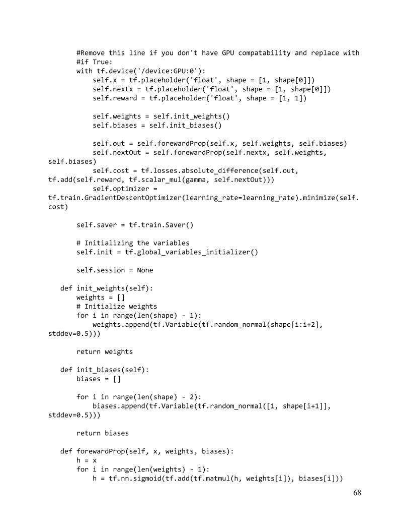
#Remove this line if you don't have GPU compatability and replace with #if True: with tf.device('/device:GPU:0'): self.x = tf.placeholder('float', shape = [1, shape[0]]) self.nextx = tf.placeholder('float', shape = [1, shape[0]]) self.reward = tf.placeholder('float', shape = [1, 1]) self.weights = self.init_weights() self.biases = self.init_biases() self.out = self.forewardProp(self.x, self.weights, self.biases) self.nextOut = self.forewardProp(self.nextx, self.weights, self.biases) self.cost = tf.losses.absolute_difference(self.out, tf.add(self.reward, tf.scalar_mul(gamma, self.nextOut))) self.optimizer = tf.train.GradientDescentOptimizer(learning_rate=learning_rate).minimize(self.cost) self.saver = tf.train.Saver() # Initializing the variables self.init = tf.global_variables_initializer() self.session = None def init_weights(self): weights = [] # Initialize weights for i in range(len(shape) - 1): weights.append(tf.Variable(tf.random_normal(shape[i:i+2], stddev=0.5))) return weights def init_biases(self): biases = [] for i in range(len(shape) - 2): biases.append(tf.Variable(tf.random_normal([1, shape[i+1]], stddev=0.5))) return biases def forewardProp(self, x, weights, biases): h = x for i in range(len(weights) - 1): h = tf.nn.sigmoid(tf.add(tf.matmul(h, weights[i]), biases[i]))

68

h = tf.add(h, tf.multiply(tf.constant([[-0.5]]), tf.ones([h.shape[0]]))) return tf.matmul(h, weights[len(weights)-1]) def train(self): # Launch the graph #self.session = tf.Session() self.load(saveLoc) self.session.run(self.init) step = 0 loss_total = 0 while step < training_iters: tIn, tNextIn, change = self.loader.getData(num_input) reward = change #reward -= trade * 10 reward = np.array([[reward]]) _, loss, pred, nxout = self.session.run([self.optimizer, self.cost, self.out, self.nextOut], \ feed_dict={self.x: tIn, self.nextx: tNextIn, self.reward: reward}) loss_total += loss step += 1 if step % display_step == 0: print("Iter= " + str(step) + ", Average Loss= " + "{:.6f}".format(loss_total/display_step)) print("Change of %f, reward of %f"%(change, reward[0][0])) print("Predicted: %f, Next: %f, loss: %f"%(pred[0][0], nxout[0][0], loss)) print("\n") loss_total = 0 self.saver.save(self.session, saveLoc) self.saver.save(self.session, saveLoc) self.session.close() def makeTrade(self, tIn, step): #make random trade if True: #No trade if random.random() < 0.5: return 0

69

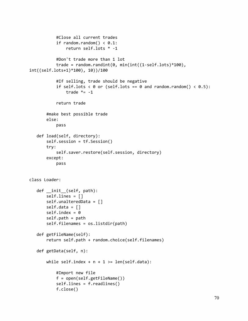
#Close all current trades if random.random() < 0.1: return self.lots * -1 #Don't trade more than 1 lot trade = random.randint(0, min(int((1-self.lots)*100), int((self.lots+1)*100), 10))/100 #If selling, trade should be negative if self.lots < 0 or (self.lots == 0 and random.random() < 0.5): trade *= -1 return trade #make best possible trade else: pass def load(self, directory): self.session = tf.Session() try: self.saver.restore(self.session, directory) except: pass class Loader: def __init__(self, path): self.lines = [] self.unalteredData = [] self.data = [] self.index = 0 self.path = path self.filenames = os.listdir(path) def getFileName(self): return self.path + random.choice(self.filenames) def getData(self, n): while self.index + n + 1 >= len(self.data): #Import new file f = open(self.getFileName()) self.lines = f.readlines() f.close()

70

self.data = [] self.unalteredData = [] for i in range(len(self.lines)): self.lines[i] = self.lines[i].split(',') self.lines[i] = self.lines[i][1:5]#Open, High, Low, Close nl = [] for j in self.lines[i]: nl.append(float(j)*10000) self.unalteredData.append(nl) for i in range(len(self.unalteredData)): if i > 1: nl = [] #Open = open-prevClose nl.append(self.unalteredData[i][0]-self.unalteredData[i-1][3]) #High = high-open nl.append(self.unalteredData[i][1]-self.unalteredData[i][0]) #Low = close-low nl.append(self.unalteredData[i][3]-self.unalteredData[i][2]) #Close = open-close nl.append(self.unalteredData[i][0]-self.unalteredData[i][3]) self.data.append(nl) self.index = 0 #Open, High, Low, Close tIn = self.data[self.index:self.index+n] tIn = np.reshape(np.array(tIn), [1, n*BARSIZE]) tNextIn = self.data[self.index+1:self.index+n+1] tNextIn = np.reshape(np.array(tNextIn), [1, n*BARSIZE]) change = self.data[self.index+n+1][0]-self.data[self.index+n+1][3] self.index += 1 return tIn, tNextIn, change if __name__ == "__main__": trainer = Trainer()

71

print("Beginning Training") #trainer.train() trainer.load(saveLoc) sumReward = 0 out = [] for _ in range(1000): tIn, tNextIn, change = trainer.loader.getData(num_input) pred = trainer.session.run(trainer.out, feed_dict = {trainer.x: tIn}) reward = pred[0][0] * change sumReward += reward out.append([change, pred[0][0]]) print("Total reward received: %f"%sumReward) for i in out: print("%f,%f"%(i[0], i[1]))

72