
FOREST MACHINERY PRODUCTIVITY STUDY WITH DATA MINING
77
School of Engineering Science Business Analytics Master’s Thesis FOREST MACHINERY PRODUCTIVITY STUDY WITH DATA MINING Juho Haapalainen Supervisors: Prof. Pasi Luukka D.Sc. (Tech.) Mika Aalto
Transcript of FOREST MACHINERY PRODUCTIVITY STUDY WITH DATA MINING

School of Engineering Science
Business Analytics
Master’s Thesis
FOREST MACHINERY PRODUCTIVITY STUDY WITH DATA
MINING
Juho Haapalainen
Supervisors: Prof. Pasi Luukka
D.Sc. (Tech.) Mika Aalto

ABSTRACT
Author: Juho Haapalainen
Title: Forest machinery productivity study with data mining
Year: 2020
School: LUT School of Engineering Science
Degree program: Business Analytics (MBAN)
Supervisors: Prof. Pasi Luukka,
D.Sc. (Tech.) Mika Aalto
Contents: 77 pages, 15 figures, 6 tables, 19 equations and 3 appendices
Keywords: forest machinery, productivity, data mining, regression, Lasso
In this thesis, multidimensional sensor data from Ponsse Oy’s harvesters were utilized with
data mining in order 1) to study the factors affecting harvesting productivity and 2) to
discover the work stages of a harvester. As the data consisted of 9.6 million time-series
observations, which had been collected from 58 sensors in 0.02 second intervals, the material
for the study corresponded to over 53 hours of harvesting work, during which more than 2,6
thousand trees had been felled.
Using Python programming language, a comprehensive data preprocessing and feature
extraction algorithm was developed for these data. The algorithm took the raw csv-files, used
the sensor information on the harvester motions to identify five work stages (felling,
processing, moving, delays and other activities) from the time-series data, and
simultaneously, by extracting a set of 17 explanatory variables, gradually built a data frame,
in which the rows corresponded to the temporal sequences, during which an individual tree
had been felled and processed (including possible movement from the previous tree). To
determine the most important factors affecting harvesting productivity, regression analysis
was then conducted on this preprocessed dataset. Firstly, after an automated feature selection
with backward elimination, OLS multiple regression was fitted both with standardized (𝜇 =0 and 𝜎2 = 1) and Box-Cox-transformed values. R-squared values of 0.74 and 0.84,
respectively, were obtained for these two models, and their validities were studied with
selected statistical tests, including Koenker, Durbin-Watson and Jarque–Bera tests. Also,
Lasso regression, with grid-search cross-validation based optimization of the penalty
parameter λ, was fitted, and this time R-squared value of 0.77 was obtained.
As a result of this thesis, eight factors affecting harvesting productivity were discovered,
including the diameter of the felled tree, the temporal shares of felling and processing (i.e.
delimbing and cross-cutting) from the total work time, average fuel consumption, tree
species, inter-tree distance, crane movement complexity and the moving average of the
harvesting productivity. By far the most important factor (with standardized coefficients from
0.73 to 0.77) was the tree diameter, as opposed to the other seven factors with coefficients
from 0.05 up to 0.23. The factors that did not seem to affect the productivity include, for
instance, the altitude changes, the driving speed between the trees and the time since starting
the current fellings.

3
TABLE OF CONTENTS
1 INTRODUCTION ..................................................................................................... 6
2 FOREST MACHINERY PRODUCTIVITY ........................................................... 10
2.1 The process of literature review ............................................................................... 10
2.2 The definition and motivation of forest machinery productivity ............................. 11
2.3 The factors affecting forest machinery productivity ................................................ 12
2.4 Harvester work stages .............................................................................................. 14
3 DATA MINING ....................................................................................................... 16
3.1 Data collection ......................................................................................................... 17
3.2 Data preprocessing ................................................................................................... 17
3.3 Analytical processing ............................................................................................... 20
4 THEORY ON REGRESSION ANALYSIS ............................................................ 23
4.1 Least-squares estimated multiple linear regression ................................................. 23
4.2 Standard assumptions of the OLS model ................................................................. 24
4.3 Regression metrics ................................................................................................... 27
4.4 Lasso regression ....................................................................................................... 28
5 FELLINGS, SITE AND MACHINERY ................................................................. 30
6 HARVESTER DATA COLLECTION AND PREPROCESSING ......................... 33
6.1 Collecting harvester data .......................................................................................... 33
6.2 Workflow of data preprocessing .............................................................................. 34
6.3 Identifying harvester work stages ............................................................................ 35
6.4 Feature extraction ..................................................................................................... 39
7 REGRESSION ANALYSIS ON HARVESTER DATA ......................................... 41
7.1 Feature selection and OLS multiple regression ....................................................... 41
7.2 Regression with Box-Cox transformed values ........................................................ 45
7.3 Lasso regression ....................................................................................................... 48

4
8 EMPIRICAL RESULTS .......................................................................................... 50
9 DISCUSSION .......................................................................................................... 54
9.1 On the methods and results ...................................................................................... 54
9.2 Scientific contributions and suggested directions of further research ..................... 56
10 SUMMARY AND CONCLUSIONS ...................................................................... 58
REFERENCES ......................................................................................................................... 60
APPENDICES .......................................................................................................................... 68
A1 Metadata of the collected harvester log files ................................................................ 68
A2 Python code: Regression analysis ................................................................................. 70
A3 Python code: Data preprocessing and feature extraction .............................................. 74

5
LIST OF FIGURES
Figure 1 Phases of data mining ................................................................................................ 16
Figure 2 Boom-corridor thinning work-patterns ..................................................................... 30
Figure 3 Ponsse Scorpion King harvester ................................................................................ 31
Figure 4 Locations of the sites in South-Eastern Finland ........................................................ 32
Figure 5 Illustration of the data preprocessing algorithm workflow ....................................... 34
Figure 6 Illustrative sketch of the work stage identification ................................................... 36
Figure 7 Lengths of the identified work stages in seconds ...................................................... 38
Figure 8 Illustration of division between harvester work cycles ............................................. 39
Figure 9 Backward elimination algorithm for feature selection .............................................. 42
Figure 10 Multicollinearity removal algorithm ....................................................................... 42
Figure 11 The process of eliminating the redundant and intercorrelated features .................. 43
Figure 12 Heatmap of matrix of bivariate Pearson’s correlations ........................................... 43
Figure 13 Scatter plot of observed vs. predicted values & histogram of model residuals ...... 45
Figure 14 Observed vs. predicted values and the residuals distribution after Box-Cox.......... 46
Figure 15 The most important variables affecting harvesting productivity ............................ 50
LIST OF TABLES
Table 1 Harvester work stages used in different studies.......................................................... 15
Table 2 Work stage definitions used in the current study ........................................................ 37
Table 3 List of features in the extracted data frame................................................................. 40
Table 4 Results of OLS multiple regression ............................................................................ 44
Table 5 Results of OLS multiple regression with Box-Cox transformed values ..................... 47
Table 6 Coefficients in Lasso regression ................................................................................. 49

6
1 INTRODUCTION
Due to advancements in information technology, huge volumes of data can nowadays be
collected from various types of physical devices. Alongside with the growing amount of data,
new methods of data mining are continuously developed in order to achieve better
comprehension of the stored information. Increasing amount of industries are becoming data-
driven, and already a quick literature review shows that forestry sector is not an exception: data
mining methods have been used to analyze or estimate, for instance, forest stand attributes
(Yazdani et al., 2020), carbon storage in the trees (Corte et al., 2013), tree density and
biodiversity (Mohammadi et al., 2011), burned area in forest fires (Özbayoglu and Bozer, 2012)
and the factors responsible for deforestation (Mai et al., 2004).
Modern forest machines are increasingly often equipped with extended logging and data
collection systems. With embedded sensors, various types of information regarding the
motions, expenditures and performance of the harvester are produced as the by-product of the
harvesting operations. The potential use areas and applications of these data are numerous,
including harvesting site planning, wood purchasing and site classification, as well as quality
models and control of bucking (Räsänen, 2018). Insightful applications can also be developed
when the harvester data is integrated with data from other sources. Olivera (2016), for example,
explored the opportunities of integrating harvester data with satellite data to improve forest
management, whereas Saukkola et al. (2019) used harvester data with airborne laser scanning
and aerial imagery in predicting the forest inventory attributes.
But how could harvester data be utilized in order to examine and develop harvesting
productivity? Having a set of sensor data collected from Ponsse Oy’s harvesters, that was the
particular question which led to this thesis. As a part of a PUUSTI research project aiming to
study and demonstrate a new technique, boom-corridor thinning, several fellings were
conducted. During this process, values of tens of different sensors were recorded from
harvesting activities by using a data collection software developed by Creanex Oy, yielding
large amounts of multidimensional time-series data. The data were massive both in terms of
size and scope, offering a wide array of alternative research directions. After considering

7
several other utilization possibilities, the specific research question, which turned out being
both feasible and the most meaningful to be answered, was the following:
Research question no. 1:
Based on these data, what are the factors affecting harvesting productivity?
Harvesting productivity, defined as the volume of harvested wood per a unit of time, is
generally calculated by the collection of empirical field data. Several academic papers have
been published regarding the factors influencing it, and a strong consensus exists among
researchers that the most important one is the average quantity of wood that each harvested tree
contains. Many other factors, however, have an impact on productivity as well, for instance
technical capability of the harvester, tree species, stand density, weather and other seasonal
conditions, terrain as well as road spacing and condition (Langin et al., 2010). Also, experience
level of the operator (Lee et al., 2019; Purfürst and Erler, 2011), forwarder load capacity
(Eriksson and Lindroos, 2014) and the work shift (Rossit et al., 2019, 2017) can explain
variation in harvesting productivity. But what would be the most important factors based on
these particular set of data? The aim here was to study and quantify the impact of both the
factors that were found in the literature (for those that the scope of the data allowed), and if
possible, find some new affecting factors as well.
To answer its research questions, extensive data mining is used in this thesis. But what does it
mean to mine data, and how it is different from the ordinary mining, which aims to find precious
metals from the soil? Well, the common denominator between them is that they both search for
something valuable from a great deal of raw material. In the case of data mining, the valuable
thing is knowledge: interesting interpretations, hidden patterns or useful insights from the data
that increase the understanding of some topic. Data mining is a highly general umbrella term,
that covers a myriad techniques and algorithms to process and analyze data, each of which is
best suited to some very specific problem. In the context of this thesis, data mining meant data
preprocessing and regression analysis. In the data preprocessing part, the set of raw harvester
log data files were taken, and by cleaning, integrating and transforming them, the factors, whose
impact on harvesting productivity could be studied, were extracted into a single, clean dataset.
Then, in the regression analysis part, three linear models, least squares estimated multiple linear

8
regression (both with standardized and Box-Cox transformed values) and Lasso (Least absolute
shrinkage and selection operator) regression, were fit to these data to quantify the impact of
these factors on the harvesting productivity. The whole data mining pipeline was implemented
using Python programming language, which is known as a high-level, general-purpose and
widely-used programming language with easy-to-use data processing and visualization libraries
(e.g. Pandas, NumPy, Matplotlib).
Research question no. 2:
Which work stages can be identified from these harvester data and how?
During the research process, another interesting question appeared, and as answering it served
the purposes of the main research question, it was included in the scope of this thesis. Harvester
work stages, such as movement of the machine, positioning the harvesting head, felling a tree
and delimbing and cross-cutting the stem, are the key actions from which the workflow of a
harvester constitutes. By exclusively defining these temporal elements, the operation of a forest
machine can be viewed as a series of subsequent stages. When a field, indicating the harvester
work stage currently in progress, is included in the time-series data, the time consumption of
these work stages can be systematically measured and used to study the productivity of the
harvesters. In earlier studies the information regarding the current temporal element has been
recorded by a human, but in the present study, due to fully automatic data collection, the work
stage information was not available. Hence, a system, which could be used to classify the time-
series points into the work stages, needed to be developed.
The results of this thesis must be considered together with the limitations of the study. Firstly,
despite the plurality of the sensors that were used in the data collection, the scope of the data
used for this study were still limited. Several factors, for example experience level of the
harvester operator, terrain and road condition, weather conditions or the time of the day, whose
effect on productivity would have been interesting to determine, were not available. Moreover,
as the data were collected using only one type of harvester, the technical capability of the
machine, as a factor affecting to productivity, could not be studied. Secondly, the analytical
methods, used to determine the factors affecting on productivity, were limited to regression
analysis, and more precisely, to two specific types of regression analysis. The initial least-

9
squares model provided a good basis for its extension, Lasso regression, which was selected
due to its ability to perform variable selection by shrinking the redundant coefficients, hence
mitigating the problems imposed by multicollinearity in predictor variables. However, if other
regression methods (e.g. Ridge, Elastic-Net or Principal Component regression) or non-
regression methods (e.g. Random Forest, XGBoost, AdaBoost, Neural Networks) had been
used, the results might have differed from the ones obtained in this study. Thirdly, it is important
to notice that this thesis project has not involved observation of the fellings in any way, neither
physically on the harvested sites nor from the video. With that, validating some of the steps of
data preprocessing and feature extraction (i.e. identifying the work stages) was more difficult.
The remaining of the thesis is structured as follows. The second chapter is a literature review
regarding the factors affecting harvesting productivity and the harvester work stages. In the
third chapter, data mining is defined as a term and the general process of data mining is
presented. The fourth chapter provides a selection of theory on regression analysis and other
statistical methods that were used in this thesis. In the fifth chapter, the fellings, site and
machinery are described. In the sixth chapter, data collection and preprocessing steps (including
the work stage identification) are presented. In the seventh chapter, the regression analysis for
the harvester data is presented in detail. In the eighth chapter, the empirical findings of the
analysis are analyzed and interpreted. In the ninth chapter, discussion is provided regarding the
methods and the results of the thesis and some directions for further research are suggested. In
the tenth chapter, the thesis and its conclusions are summarized.

10
2 FOREST MACHINERY PRODUCTIVITY
How is forest machinery productivity defined? Why is productivity of the forest machines
important and how could one measure it? Which factors affect the productivity and what kind
of research methods have previously been used to study them? What are harvester work stages?
How can one distinguish between the stages and why would one want to do so? This chapter is
a literature review, and those were the main questions it aims to provide answers to.
2.1 The process of literature review
According to Taylor (2007), the aim of a literature review is to classify and evaluate the written
material on a certain topic produced by accredited scholars and researchers. Being “organized
around and related directly to the research question” of a thesis, a literature review “synthesizes
results into a summary of what is and is not known, identifies areas of controversy and
formulates questions that need further research”. Literature review demonstrates the ability of
the author both to a) seek useful information, such as articles, books and documents, by
scanning the literature in an efficient manner, and b) by applying principles of analysis, to
critically evaluate the studies and material found.
To find the source material for this literature review, a structured three-step approach by
Webster and Watson (2002) was used. A systematic search of this type, according to them,
should ensure the accumulation of a relatively complete collection of relevant literature. In
short, the idea of the approach is to 1) by using appropriate keywords and / or by searching
from the leading journals and conference proceedings, identify an initial set of relevant articles
2) go backward: by reviewing the citations in the initial set, find a set of key articles that had
served as a theoretical basis for the latter articles 3) go forward: find more relevant articles by
identifying the articles citing the key articles that had been identified in the previous steps.
Especially in the final step, the usage of selected scientific search engines is suggested.
The hunt for the relevant articles began with keywords forest machine(ry), harvester and
harvesting combined with productivity. The keywords were used to search articles from a
number of major scientific databases using the portals and search engines provided by
ResearchGate, ScienceDirect and Google Scholar. More results were obtained when the initial

11
keywords were used with phrases key factors of, factors affecting and variables influencing.
Due to the data-driven context of this study, a particular interest was focused to the articles
found with further additions data mining, data analytics and big data being attached to the
search expressions. To find articles related to harvester work stages, both the term work stage
and its synonyms - phase and - element were used as keywords. As a result of the first step, 14
relevant articles were found, and after drilling down to the original sources in the second step,
and tracing the articles that cited to them in the third step, 10 additional articles were discovered,
resulting in a total number of 24 relevant articles. Majority of these articles were from the
leading publications of the field, such as International Journal of Forest Engineering, Journal
of Forestry Research and Silva Fennica.
2.2 The definition and motivation of forest machinery productivity
According to Cambridge Dictionary (2020), productivity can be defined as “the rate at which a
country, company, etc. produces goods or services, usually judged in relation to the number of
people and the time necessary to produce them”. The term forest machine refers to various types
of vehicles. In contrast to forwarders, which are used to carry the logs to a roadside landing,
the focus of this thesis is solely on the harvesters: the vehicles employed in cut-to-length
logging operations to fell, delimb and cross-cut trees. With a few alternative measures of
harvesting productivity also being possible, the one that will be used in this thesis is the volume
of harvested wood per a unit of time.
Forest machinery productivity is generally calculated by the collection of empirical field data.
To examine the performance of the machines either time and motion studies, involving work
observation, or follow-up studies, involving analysis historical output records, can be used
(Eriksson and Lindroos, 2014). Forest machinery productivity is important from the point of
view of financial profitability, as being able to deliver requested volumes of wood at time, and
at a reasonable price, guarantees a return on investment for the harvesting contractor or
company (Langin et al., 2010). Productivity is an important aspect also for forest owners, as
fellings are often so expensive to conduct that the costs can exceed their revenues. And because
forest machinery productivity is important, it is also important to study factors affecting it.

12
2.3 The factors affecting forest machinery productivity
Numerous scientific articles have been published regarding the factors affecting forest
machinery productivity. Having data from single grip harvester Ponsse Ergo 8W from
Eucalyptus plantations in Uruguay, Rossit et al. (2019, 2017) studied how different variables
affect the productivity of a harvester; by modelling the productivity both as ranges of equal
intervals and as ranges calculated using k-means clustering, the researchers used decision trees
to determine the variables affecting the productivity. Eriksson & Lindroos (2014), on the other
hand, analyzed the productivity of cut-to-length harvesting and forwarding using large follow-
up dataset, routinely recorded by a Swedish forestry company using forest machines of several
manufacturers. In their study, a set of stand-based productivity models were constructed for
both harvesters and forwarders using least-squares estimated linear regression.
The effect of individual tree volume on operational performance of harvester processor in
northern Brazil was investigated by Rodrigues et al. (2019); by the means of a time and motion
study and regression analysis, “the time consumed in the phases of the operational cycle,
mechanical availability, operational efficiency, productivity, and production costs in three
stands with different individual mean volumes”, were determined. Lee et al. (2019) researched
the performance of log extraction by a small shovel operation in steep forests in South Korea;
having data from 30 case study areas, Pearson’s correlation test was used to clarify the effect
of different independent variables on the productivity and a predictive equation for productivity
was developed using ordinary least squares regression technique. The study of Kärhä et al.
(2013) focused on productivity, costs and silvicultural result of mechanized energy wood
harvesting from early thinnings. Using multitree-processing Naarva-Grip 1600-40, work-
studies were conducted in six young stands at the first thinning stage. By the means of
regression analysis, which used the harvesting conditions, such as density, height, and size of
removal, as independent variables, the proportion of multi-tree processing was estimated.
A consensus seems to exist among the abovementioned researchers: the most influential
variable in productivity is the quantity of wood that each harvested individual contains. Simply
put, according the research, the harvesting productivity is enhanced best by felling high-volume
tree individuals. In the study of Eriksson & Lindroos (2014), the variable best explaining the
variance in thinning and final felling productivity was mean stem size (measured in cm3),

13
whereas Rossit et al. (2019, 2017) found diameter at breast height (measured in cm) being the
most influential factor in their model. Accordingly, Rodrigues et al. (2019) concluded that the
higher the individual mean volume of the tree of the stand, the machine's productivity tended
to be higher, and the results of Lee et al. (2019) indicated that the “productivity was significantly
correlated with stem size (diameter at breast height and tree volume)”. Kärhä et al. (2013)
suggests that “in order to keep the felling-bunching costs at a reasonable level, mechanized
harvesting should be targeted at sites where the average size of the trees removed is over 30
dm3, and the energy wood volume at felling over 30 m3 /ha”.
Stem volume, however, was not the only influential factor the researchers found. Alongside
tree size, Eriksson & Lindroos (2014) successfully used mean extraction distance and forwarder
load capacity to explain 26.4% of the variance in thinnings and 35.2% in final fellings, whereas
Rossit et al. (2019, 2017) found that after setting the DBH values, new variables, such as
harvester operator, tree species and work shift, could be used describe productivity. The results
of Lee et al. (2019) indicated that “the mean extraction productivity of small-shovel operations
ranged between 2.44 to 9.85 m3 per scheduled machine hour” and that the productivity, in
addition to the stem size, was significantly correlated with total travelled distance (TTD).
Referring to the study of Purfürst and Erler (2011), one of the key components in forest
machinery productivity also seems to be the operator performance. Having data collected from
single-grip harvesters, which had been driven by 32 operators from 3,351 different stands
within a period of three years, the researchers studied the influence of human on productivity
in harvesting operations. By means of regression analysis, the researchers found that 37,3 % of
the variance in productivity can be explained by the operator, suggesting that human side should
indeed be considered as a important factor in harvesting productivity models.
The factors affecting harvesting productivity have also been listed in The South-African Ground
Based Harvesting Handbook (Langin et al., 2010). According the book, harvesting productivity
is affected by various factors, some of which are within the control of a managers in a company,
while some are not. The affecting factors are grouped into three categories: stand factors, system
factors and equipment factors. The stand factors include factors such as species, stand density,
average tree volume, terrain, road spacing and condition, weather and other seasonal conditions,

14
whereas the system factors, which address the human factor in harvesting systems, are
expressed as 5 B’s: bottlenecks, buffers, breakdowns, blunders and balances. Equipment factors
refer to the technical capability of the machines or the system used and required resources.
According to also this book, the piece size of timber to be harvested is the overall most
important factor affecting harvesting productivity. (Langin et al., 2010)
2.4 Harvester work stages
Studies of harvesting performance often involve separation between harvester work stages: the
key actions from which the workflow of a harvester constitutes, i.e. felling a tree, delimbing
and cross-cutting the stem or movement of the machine. When these repeating work elements,
as a part of a time study, are exclusively defined, one can collect data regarding the time
consumption of the stages. The workflow of a harvester at a site can then be viewed as a time
series of subsequent stages, in which one and only one work stage, by definition, takes place at
a time. The work stages used in seven different studies have been summarized in Table 1,
showing that stage definitions are not standardized in any way: different researchers have
distinguished between the stages differently – in ways, they have seen them best serving the
purposes of their studies. However, the same elements are repeated in them: in some study, the
researchers, for example, may have combined two work stages that appear as separate elements
in another study, and vice versa, or called the same work step by a slightly different name.
The collected work stage information can be used for many purposes. Di Fulvio (2012), for
instance, used the work stage information in their study regarding “productivity and
profitability of forest machines in the harvesting of normal and overgrown willow plantations”,
whereas Kärhä et al. (2013), first determined the distribution of time consumption between the
work elements and then used the obtained information to study the productivity and costs of
“mechanized energy wood harvesting from early thinnings”. The partition to work stages was
present also in the comparison study of “boom-corridor thinning and thinning from below
harvesting methods in young dense scots pine stands” by Bergström et al. (2010) as well as in
the study of Erber et al. (2016) regarding the “effect of multi-tree handling and tree-size on
harvester performance in small-diameter hardwood thinnings”.

15
Table 1 Harvester work stages used in different studies
Study / Author(s) Work stages used
Mechanized Energy Wood Harvesting from
Early Thinnings (Kärhä et al., 2013)
1) moving 2) boom-out 3) felling and collecting 4)
bunching 5) bucking 5) miscellaneous 6) delays
Effect of multi-tree handling and tree-size on
harvester performance in small-diameter
hardwood thinnings (Erber et al., 2016)
1) moving 2) felling 3) processing 4) delay
Productivity and Profitability of Forest
Machines in the Harvesting of Normal and
Overgrown Willow Plantations (Di Fulvio et
al., 2012)
1) boom out, 2) felling and accumulating, 3) boom
in, 4) moving, 5) miscellaneous, 6) delays
Comparison of Boom-Corridor Thinning and
Thinning From Below Harvesting Methods in
Young Dense Scots Pine Stands (Bergström et
al., 2010)
1) moving 2) crane-out 3) positioning and felling 4)
crane in-between 5) crane-in 6) bunching 7)
miscellaneous 8) delays
Comparison of productivity, cost and
environmental impacts of two harvesting
methods in Northern Iran: short-log vs. long-
log (Mousavi Mirkala, 2009)
1) felling 2) processing 3) skidding 4) loading 5)
hauling 6) unloading
The accuracy of manually recorded time study
data for harvester operation shown via
simulator screen (Nuutinen et al., 2008)
1) moving forward, 2) steer out the boom and grab,
3) felling, 4) delimbing and cross-cutting) 5)
reversing 6) steer the boom front and 7) pause time
Effect of tree size on time of each work
element and processing productivity using an
excavator-based single-grip harvester or
processor at a landing (Nakagawa et al., 2010)
1) swinging without tree 2) picking up 3) delimbing
whole tree 4) swinging with tree 5) determining butt-
end cut 6) cutting butt end 7) feeding and measuring
8) cross-cutting 9) tree top 10 cleaning 11) other
The work stage data is usually collected manually, by a human researcher using selected
measuring technology. Kärhä et al. (2013), for example, employed KTP 84 data logger, whereas
in the study of Di Fulvio et al. (2012) the lengths of the work stage were recorded by using
Allegro Field PC® and the SDI software by Swedish company Haglöf AB. Bergström et al.
(2010) recorded the time consumption for the felling and bunching work with a Huskey Hunter
field computer and Siwork 3 software. In the case of Erber et al. (2016) the time study was
carried out using a handheld Algiz 7 computer; moreover, they recorded a video from the
operations, which they used later on to correct the errors, hence guaranteeing error-free data.

16
3 DATA MINING
Data mining is a highly general term referring to a broad range of methods, algorithms and
technologies that are used with the “aim to provide knowledge and interesting interpretation of,
usually, vast amounts of data” (Xanthopoulos et al., 2013). In other words, it is the study of
collecting, cleaning, processing, analyzing and gaining useful insights from data, and its
methodology can be applied in a wide variety of problem domains and real-world applications
(Aggarwal, 2015). As “an interdisciplinary subfield of computer science”, data mining involves
“methods at the intersection of artificial intelligence, machine learning, statistics, and database
systems” (Chakrabarti et al., 2006). With data mining, one usually seeks to provide answers to
questions concerning both the contents and the hidden patterns of the data as well as the
possibilities to use the data for future business benefit (Ahlemeyer‐Stubbe and Coleman, 2014).
As an analogy to gold discovery from large amounts of low-grade rock material, data mining
can be thought as knowledge discovery from a great deal of raw data (Han et al., 2012).
Figure 1 Phases of data mining (Modified from Aggarwal (2015))
Data mining can be seen as a process consisting of several phases. Multiple alternative data
mining process frameworks, more or less similar to each other, have been presented in the
literature, but the one that will be used in this thesis is from Aggarwal’s (2015) book, consisting
of three main phases: data collection, data preprocessing and analytical processing. Process
diagram of this general framework is illustrated in Figure 1.

17
3.1 Data collection
The first step of the data mining process is data collection. As a term, it can be defined as “the
activity of collecting information that can be used to find out about a particular subject”
(Cambridge Dictionary, 2020) or as “the process of gathering and measuring information on
variables of interest, in an established systematic fashion that enables one to answer stated
research questions, test hypotheses, and evaluate outcomes” (Northern Illinois University,
2005). According to Aggarwal (2015), the nature of data collection is highly application-
specific. The way the data is collected is entirely determined by the task at hand, and depending
on the situation, different methods and technologies can be used, including sensors and other
measuring devices or specialized software, such as a web document crawling engines.
Sometimes also manual labor is needed, for instance, to collect user surveys. When the data has
been collected, they can be stored in a data warehouse for further processing steps.
Data collection is highly important part of the data mining process, as the choices made in it
can impact the data mining process significantly (Aggarwal, 2015). Ensuring accurate and
appropriate data collection is essential also to “maintaining the integrity of research, regardless
of the field of study” (Northern Illinois University, 2005). But despite its crucial importance,
most data mining text books, such as the ones by Ahlemeyer‐Stubbe and Coleman (2014), Han
et al. (2012) or Xanthopoulos et al. (2013), do not say much about data collection, but focus
merely on the process that starts from the point where the data has already been collected. The
reason for this may be the fact, mentioned by Aggarwal (2015), of data collection tending to be
outside of the control of the data analyst. In other words, as the person performing the data
mining often cannot influence the data collection, most authors have not seen it necessary to
address the topic in their books.
3.2 Data preprocessing
Data preprocessing, by definition, refers to a wide variety of techniques that are used to prepare
raw data for further processing steps (Famili et al., 1997). The aim of data preprocessing is to
obtain clean, final data sets which one can start analyzing using selected data mining methods
(García et al., 2016). In real-world applications, the data comes in diverse formats, and the raw

18
datasets are highly susceptible to noise, missing values and inconsistencies (Aggarwal, 2015).
Simultaneously, they tend to be huge in size and can have their origins in multiple heterogenous
sources (Han et al., 2012). Due to these reasons, almost never can one start applying analytical
methods to the data before preprocessing it first in way or another; without preparing the data,
it is unlikely for one to find meaningful insights from it using data mining algorithms
(Ahlemeyer‐Stubbe and Coleman, 2014). The importance of data preprocessing is emphasized
also by Pyle (1999), according to whom the adequate preparation of data can often make the
difference between success and failure in data mining.
As it is very common that the data for a data mining task comes from more than one source,
one of the main concepts in data preprocessing is data integration, which refers to merging and
combining data from different sources, such as different databases, data cubes or flat files. In
the best – albeit rare – case, the data in different sources are homogenous. The structural or
semantic heterogeneity in different data sources can make identifying and matching up
equivalent real-world entities from them very tricky, and undesired redundancies can take
place: either some of the features or observations may become duplicated. Also, due to
“differences in representation, scaling, or encoding”, there can be conflicts in data values, which
need to be detected and resolved before the data can be integrated. Generally speaking, good
choices in data integration can significantly reduce redundancies and inconsistencies in the
resulting dataset, thus making subsequent data mining steps easier. (Han et al., 2012)
Another major task in data preprocessing is data cleaning. One of the most typical issues in
data cleaning, the missing data, can be dealt with in numerous different ways: the records with
missing values can be eliminated, a constant value can be used to fill in the missing value or, if
possible, the missing values can be filled manually. One can also try to replace the missing
values by estimation, using different imputation strategies: simply using mean, mode or median,
or using more advanced methods such as k-nearest neighbor imputation. Another issues in data
cleaning include smoothing noisy data and identifying or removing outliers. To smooth noisy
data, techniques such as regression and binning can be used. To deal with outliers, different
supervised methods (learning a classifier that detects outliers), unsupervised methods (e.g.
clustering) and statistical approaches (detecting outliers based on distributions) can be used.
(Ahlemeyer‐Stubbe and Coleman, 2014; Han et al., 2012)

19
Data preprocessing also involves feature extraction. In feature extraction, the original data and
its features are used in order to derive a set of new features that the data mining analyst can
work with. Formally, one could define feature extraction as taking original set of features
𝐴1, 𝐴2, … , 𝐴𝑛, and as a results of applying some functional mapping 𝐹, obtaining another set of
features 𝐵1, 𝐵2, … , 𝐵𝑚 where 𝐵𝑖 = 𝐹𝑖(𝐴1, 𝐴2, … , 𝐴𝑛) and 𝑚 < 𝑛. As data has a manifold of
different formats and types, feature extraction is a highly application-specific step – off-the-
shelf solutions are usually not available for doing it. For instance, image data, web logs, network
traffic or document data need completely different feature extraction methods. Feature
extraction is needed especially when data is in raw and unstructured form, and in complex on-
line data analysis applications that have a high number of measurements that correspond to a
relatively low number of actual events. In the case of sensor data, which is often collected as
large volumes of low-level signals, different transformations can be used to port time-series
data into multidimensional data. (Aggarwal, 2015; Famili et al., 1997; Motoda and Liu, 2002)
Feature extraction should not be confused with another concept of feature selection. Motoda
and Liu (2002) make a clear terminological distinction: feature selection is “the process of
choosing a subset of features from the original set of features” in a way that the feature space
is optimally reduced, as opposed to feature extraction, in which a set of new features are created
based on the original data. However, by specifying the creation of new features as the distinctive
trait of feature extraction, the definition gets very close to the one of feature construction, which
can be defined as constructing and adding new features from the original set of features to help
the data mining process (Han et al., 2012).
Feature construction, despite the fact that one can hear the terms being used interchangeably by
data mining practitioners, should not either be confused with feature extraction. To make the
difference in this thesis, let us again refer to Motoda and Liu (2002): in feature construction,
the feature space is enlarged, whereas feature extraction results in a smaller dimensionality than
the one of the original feature set. The definitions, however, are not unambiguous even in
scientific literature, which is shown by an interesting controversy: according to Sondhi (2009),
feature construction methods, that involve generating new and more powerful features by
transforming a given set of input features, may be applied to reduce data dimensionality, which
is the exact opposite to what Motoda and Liu (2002) stated about the topic.

20
The goal in both feature extraction and feature selection is to reduce the number of dimensions
in the data, whilst simultaneously preserving the important information in it. To refer to both
terms, one can use the hypernym dimensionality reduction, which according to Han et al.
(2012), can be defined as applying data encoding schemes to obtain compressed representation
of the original data. Two of the most typical dimensionality reduction techniques, principal
component analysis (PCA) and singular value decomposition (SVD), are based on axis-
rotation: by identifying the sources of variation in the data, they “reduce a set of variables to a
smaller number of components” (Aggarwal, 2015; Ahlemeyer‐Stubbe and Coleman, 2014).
Another group of methods that can be used to reduce the dimensionality are different linear
signal processing techniques, such as discrete wavelet (DWT) or Fourier transforms (DFT)
(Han et al., 2012).
There is also the term data reduction, which can refer to both the reduction observations and
dimensions (Aggarwal, 2015; Han et al., 2012). Typical methods to reduce the number of
observations include sampling and filtering (Pyle, 1999) as well as techniques such as vector
quantization or clustering, which can be used to select relevant data from the original sample
(Famili et al., 1997). Data reduction is a broad concept and it can be performed in diverse
manners: in the simplest case, it involves feeding the data through some pre-defined
mathematical operation or function, but often one needs code scripts that are fully customized
for the task at hand. These approaches, aiming to minimize the impact of the large magnitude
of the data, can also be referred to as Instance Reduction (IR) techniques (García et al., 2016).
3.3 Analytical processing
After collecting and preprocessing the data, one can start applying analytical methods on it. To
give a broad overview on what kind of techniques exist, let us present the categorization
provided by Fayyad et al. (1996), according to whom the analytical methods in data mining can
be put into six general classes of tasks:
1. Classification: mapping the observations into a set of predefined classes using a classifier
function. For instance, naïve Bayes (Domingos and Pazzani, 1997), logistic regression

21
(Berkson, 1944), decision trees (Quinlan, 1986) or support vector machines (Cortes and
Vapnik, 1995) can be used for these purposes.
2. Regression: mapping the observations to a to a real-valued prediction variable using a
regression function. In addition to ordinary least-squares estimated linear regression, Lasso
regression (Tibshirani, 1996), Ridge regression (Hoerl and Kennard, 1970) and partial least-
squares regression (Kaplan, 2004), for instance, can be used.
3. Clustering: discovering groups of similar observations in the data. The most commonly used
techniques of clustering include k-means (MacQueen, 1967) as well as different types of
hierarchical (Defays, 1977) and density-based (Ester et al., 1996) clustering. One of the
latest methods, designed for time-series data, is Toeplitz Inverse Covariance-Based
Clustering (Hallac et al., 2017).
4. Summarization: finding a more compact description for the data, using e.g. multivariate
data visualizations and summary statistics (such as mean, standard deviation or quantiles).
Summarization is often used as a part of exploratory data analysis. (Fayyad et al., 1996)
5. Association rule learning: searching for dependencies and relationships between variables.
For instance, market basket analysis (Kaur and Kang, 2016) can be used define products
that are often bought together, and text mining (Hearst, 1999) to identify co-occurring terms
and keywords. This class of tasks can also be called as dependency modeling.
6. Anomaly detection: identifying unexpected, interesting or erroneous items or events in data
sets. Also referred to as outlier/change/deviation detection. Different clustering-,
classification- and nearest neighbor-based approaches can be utilized alongside with
statistical and information theoretic methods (Sammut and Webb, 2017).
The above categorization, however, is not one of its kind. Especially in the business context,
the analytical methods in data mining are often referred to as analytics, which according to
Greasley (2019), can be divided into three classes:

22
1. Descriptive analytics tell what has happened in the past. By the means of different kind of
reports, metrics, statistical summaries and visualizations, such as graphs and charts,
descriptive methods present the data as insightful, human-interpretable patterns, which aim
to explain and understand the bygone events and performance. Descriptive analytics could
be used, for example, to examine the past trends in sales revenues.
2. Predictive analytics refer to forecasting and anticipating the future events based on historical
data. This is commonly done by using different machine learning models, which predict the
values of a target variable based on the values of a set of explanatory variables. Predictive
analytics are used, for instance, in maintenance: by predicting the possible breakdown of an
industrial machine, the machine can proactively be maintained already before it breaks,
which can help the company to save large amounts of resources.
3. Prescriptive analytics are used to recommend a choice of action. As opposed to predictive
analytics, which merely tell what will happen in the future, prescriptive analytics also tell
that what should be done based on that information. The recommendations are usually done
by optimization: by maximizing or minimizing some aspect of performance, typically
business profit in some form. An industrial company, for instance, might use prescriptive
analytics to determine optimal manufacturing and inventory strategy.
Even though there is a vast amount of different analytical methods available, it is important to
remember that each data mining application is one of its kind. Creating general and reusable
techniques across different applications can thus be very challenging. But despite the fact that
two exactly similar applications cannot be found, many problems, fortunately, constitute of
similar kind of elements. By practical experience, an analyst can thus learn to construct
solutions to them by utilizing the general building blocks of data mining, as opposed to
reinventing the wheel every time. (Aggarwal, 2015)

23
4 THEORY ON REGRESSION ANALYSIS
Regression analysis, with its numerous variations and extensions, is one of the most commonly
used method in statistics (Mellin, 2006). The aim of regression analysis is to estimate the
relation between a dependent variable (also known as response, target, outcome or explained
variable) and one or more independent variables (also known as covariates, predictors, features
or explanatory variables) (Fernandez-Granda, 2017). The models with single predictor are often
called simple linear regression, whereas the models with a number of explanatory variables are
usually referred to as multiple linear regression (Lane et al., 2003). Regression models can also
be classified by their functional shape; there are linear models, in which the dependent variable
is modelled as a linear combination of the predictor variables, and nonlinear models, which are
nonlinear in their parameters (Everitt and Skrondal, 2010).
4.1 Least-squares estimated multiple linear regression
Let us consider a dataset (𝑿, 𝒚), where 𝒚𝑇 = [𝑦1, 𝑦1, … , 𝑦𝑛] are the responses and 𝑿 is a
𝑛 × (𝑞 + 1) matrix given by
𝑿 =
[ 𝒙1
𝑇
𝒙2𝑇
⋮𝒙𝑛
𝑇] =
[ 1 𝑥11 𝑥12 ⋯ 𝑥1𝑞
1 𝑥21 𝑥22 ⋯ 𝑥2𝑞
1 ⋮ ⋮ ⋮ ⋮1 𝑥𝑛1 𝑥𝑛2 ⋯ 𝑥𝑛𝑞]
(1)
The multiple linear regression model (Fernandez-Granda, 2017) for 𝑛 observations and 𝑞
features can be written as
𝒚 = 𝑿𝜷 + 𝝐 (2)
Where 𝝐𝑇 = [𝜖1, 𝜖2, … , 𝜖𝑛] contains the residuals, also known as error terms and 𝜷𝑇 =
[𝛽0, 𝛽1, 𝛽2, … , 𝛽𝑞] are the regression coefficients. The first parameter 𝛽0 is the intercept term,
value of 𝑦 when all other parameters are set to zero. The expected value 𝐸 of the 𝑖’th entry can
thus be calculated as

24
𝐸(𝑦𝑖) = 𝒙𝑖𝑇𝜷 + 𝜖𝑖 = 𝛽0 + 𝛽1𝑥𝑖1 + 𝛽2𝑋𝑖2 + ⋯𝛽𝑞𝑋𝑖𝑞 (3)
To fit the multiple linear regression model, one needs to estimate the weight vector 𝜷 so that it
fits the data as well as possible. The most common method is to minimize the sum of squared
errors, calculated from the differences between the observed response value and the model’s
prediction (Everitt and Skrondal, 2010).
𝑆𝑆𝐸 = ∑(𝑦𝑖 − 𝒙𝑖𝑇𝜷)2
𝑛
𝑖=1
= ‖𝒚 − 𝑿𝜷‖2 (4)
The ordinary least-squares (OLS) estimate �̂� is then
�̂� = argmin‖𝒚 − 𝑿𝜷‖2 (5)
To solve �̂�, either computational methods, or the following closed form solution can be used
�̂� = (𝑿𝑇𝑿)−1𝑿𝑇𝒚 (6)
4.2 Standard assumptions of the OLS model
The least-squares estimation cannot be used in every situation. Mellin (2006) lists six standard
assumptions, which guarantee that OLS estimation can (and also should) be used to estimate
the model. When these conditions are fulfilled, the least squares estimator, based on Gauss-
Markov theorem, is the best linear unbiased estimator, and no other estimators are needed
(Brooks, 2014).
1. Values of the predictor variables in 𝑿 are fixed, i.e. non-random constants for all i =
1, 2, . . . , n and j = 1, 2, . . . , q.
2. Variables used as predictors do not have linear dependencies with each other.

25
3. All residuals (error terms) have same expectation value, i.e. 𝐸(𝜖𝑖) = 0 for all i = 1, 2, . . . , n.
The assumption guarantees that no systematic error was made in the formulation of the
model.
4. Model is homoscedastic, that is, all residuals have same variance 𝑉𝑎𝑟(𝜖𝑖) = 𝜎2. If the
assumption is not valid, the error terms are heteroscedastic, which makes the OLS estimates
inefficient.
5. Residuals are uncorrelated with each other, i.e. 𝐶𝑜𝑟(𝜖𝑖, 𝜖𝑘), 𝑖 ≠ 𝑘. Correlation makes OLS
estimates inefficient – even biased.
6. Models residuals are normally distributed, i.e. 𝜖𝑖~𝑁(0, 𝜎2).
The latter three of these six assumptions can be statistically tested. For the 4th assumption,
Breusch-Pagan test can be tested used. The idea behind the test is to estimate an auxiliary
regression of a form 𝑔𝑖 = 𝒛𝑖𝑇𝜶, where 𝑔𝑖 = 𝜖�̂�
2 �̂�2⁄ , in which �̂�2 = ∑𝜖�̂�2 𝑛⁄ is the maximum
likelihood estimator of 𝜎2 under homoscedasticity. Usually, the original independent variables
𝒙 are used for 𝒛. To test 𝐻0: 𝛼1 = ⋯ = 𝛼𝑞 versus the alternative hypothesis of residuals being
heteroscedastic as a linear function of the explanatory variables, the Lagrangian multiplier
statistic 𝐿𝑀, which is be found as one half of the explained sum of squares in a regression, is
calculated. Under the null hypothesis 𝐻0 of residual variances being all equal, the test statistic
is asymptotically distributed as 𝜒2 with 𝑞 degrees of freedom. (Breusch and Pagan, 1980, 1979)
The problem with test statistic 𝐿𝑀 is that it crucially depends on the assumption that the
estimated residuals 𝜖𝑖 are normally distributed (Lyon and Tsai, 1996). To deal with this
problem, Koenker (1981) suggested a Studentized version of the Breusch-Pagan test, which
attempts to improve the power of the original test and make the it more robust to non-normally
distributed error terms (Baltagi, 2011). The Studentized test statistic 𝐿𝑀𝑆 can be calculated as
𝐿𝑀𝑆 =2�̂�4𝐿𝑀
�̂� (7)
where �̂� denotes the second sample moment of the squared residuals, given by

26
�̂� = ∑ (𝜖𝑖2�̂�2)2 𝑛⁄
𝑛
𝑖=1 (8)
The 5th assumption can be tested using Durbin-Watson test. The null hypothesis is that the
residuals are serially uncorrelated, and alternative hypothesis is that they follow an
autoregressive process of first order. The test statistic is given by
𝑑 =∑ (𝜖𝑖 − 𝜖𝑖−1)
2𝑛𝑖=2
∑ 𝜖𝑖2𝑛
𝑖=2
(9)
The obtained value 𝑑 is compared to upper and lower critical values, 𝑑𝑈 and 𝑑𝐿, which have
been tabulated for different sample sizes 𝑛, significance levels 𝛼 and numbers of explanatory
variables 𝑞. The decision rules for 𝐻0: 𝜌 = 0 versus 𝐻1: 𝜌 ≠ 0 are the following
If 𝑑 < 𝑑𝐿 reject 𝐻0: 𝜌 = 0
If 𝑑 > 𝑑𝑈 do not reject 𝐻0: 𝜌 = 0
If 𝑑𝐿 < 𝑑 < 𝑑𝑈 test is inconclusive
(10)
If one would like to test for negative autocorrelation (which is much less frequently encountered
than positive autocorrelation) the test statistic 4 − 𝑑 could be used with the same decision rules
as for positive autocorrelation. (Durbin and Watson, 1951, 1950).
To test the normality of residuals (6th assumption), the Jarque–Bera test can be used. The idea
behind it is to test whether the skewness and kurtosis of the residuals match the normal
distribution. The test statistic 𝐽𝐵 is defined by
𝐽𝐵 =𝑛
6(�̂�1 +
(�̂�2 − 3)2
4) (11)
�̂�1 =�̂�3
2
�̂�23 , �̂�2 =
�̂�4
�̂�22
(12)

27
where �̂�1 and �̂�2, respectively, denote the skewness and kurtosis sample coefficients, �̂�𝑖 being
the estimate of the 𝑖’th central moment. If the residuals are normally distributed (𝐻0), the test
statistic follows 𝜒2 with two degrees of freedom. (Jarque and Bera, 1987)
4.3 Regression metrics
Several metrics have been developed for evaluating the goodness and accuracy of a linear
regression model. One of the most commonly used is R-squared, also known as coefficient of
determination, which can be defined as the square of the correlation coefficient between two
variables (Everitt and Skrondal, 2010). Values of R-squared always vary between 0 and 1; the
larger the value, the larger proportion of the variance in the target variable is explained by the
predictor variable or variables (Mellin, 2006). Let abbreviation 𝑆𝑆𝐸 denote the sum of squared
errors and 𝑆𝑆𝑇 stand for the total sum of squares. The formula for R-squared is given by
𝑅2 = 1 −SSE
SST= 1 −
∑ 𝜖𝑖2𝑛
𝑖=1
∑ 𝑦𝑖2𝑛
𝑖=1
= 𝐶𝑜𝑟𝑟(𝑦, �̂�)2 (13)
R-squared, however, works as intended only with one explanatory variable model. Although it
indeed is a measure of the goodness of an estimated regression, R-squared, calculated as above,
should not be used as a selection criterion of model when multiple predictor variables are
present. Since OLS minimizes the sum of squared errors, adding more independent variables to
a model can never increase the residual sums of squares, making 𝑅2 non-decreasing (Baltagi,
2011). Let 𝐾 tell how many independent variables there are in the model, excluding the
constant. To penalize the model for additional variables, one can use adjusted R-squared, which
can be calculated as
�̅�2 = 1 −∑ 𝜖𝑖
2𝑛𝑖=1 (𝑛 − 𝐾)⁄
∑ 𝑦𝑖2𝑛
𝑖=1 (𝑛 − 1)⁄ (14)
The value of adjusted 𝑅2 is always smaller or equal to the non-adjusted 𝑅2, and the relationship
between them, as Baltagi (2011) denotes it, can be expressed by the following equation

28
(1 − �̅�2) = (1 − 𝑅2)(𝑛 − 1
𝑛 − 𝐾) (15)
Another measure of quality of an regression model is Mean Squared Error (𝑀𝑆𝐸), which is the
expected value of the square of the difference between the estimated and the true value (Everitt
and Skrondal, 2010). The value of 𝑀𝑆𝐸 is always non-negative, and the smaller the value, the
better, zero being the optimum. The formula for 𝑀𝑆𝐸 is given by
𝑀𝑆𝐸 = ∑ (𝑦𝑖 − �̂�𝑖)2
𝑛
𝑖=1= ∑ 𝜖𝑖
2𝑛
𝑖=1 (16)
In addition to 𝑅2 and 𝑀𝑆𝐸, many other metrics, such as Mean Absolute Error (𝑀𝐴𝐸), Root
Mean Squared Error (𝑅𝑀𝑆𝐸) and Mean absolute percentage error (𝑀𝐴𝑃𝐸), could be used as
well. In some articles, dozens of different metrics have been used: for example in the study of
Kyriakidis et al. (2015) in which 24 different metrics were used. The general perception in
literature seems to be that no metric is superior in all situations. As in every statistical measure
a great deal of information is compressed into a singular a value each of them gives only one
projection of model errors, which emphasizes some specific of the model performance (Chai
and Draxler, 2014).
4.4 Lasso regression
The simplicity of the least-squares estimation has its own drawbacks, namely, low prediction
accuracy and low interpretability. Low prediction accuracy, in this case, is caused by the
phenomenon called overfitting, to which OLS is highly prone to. With overfitting, one refers to
the tendency of a model to adapt to the noise or random fluctuations in the training data in a
way that the model performance on new data to decreases. The ability of an overfitted model
to capture the regularities in the training data is high, but it generalizes poorly on unseen data.
Low interpretability means here that least-squares estimation produces a complex model with
a huge number of predictors. To increase the interpretability, one would like to a determine a
small subset of variables having the strongest contribution to the target. (Tibshirani, 1996)

29
To overcome the problems mentioned above, a penalized least squares regression method Lasso
(Least Absolute Shrinkage and Selection Operator) can be used (Tibshirani, 1996). To prevent
the model from overfitting, Lasso uses regularization: an extra penalty term is added to the error
function, and with the growing magnitude of the regression parameters, there will be an
increasing penalty cost function (Bühlmann and van de Geer, 2011). Let 𝑿, 𝒚 and 𝜷 be similar
as in previous subchapter and let 𝜆 denote the penalty parameter that controls the amount of
shrinkage applied to the estimate. The of Lasso estimator �̂�, in its basic form, is defined by
�̂� = argmin{∑(𝑦𝑖 − 𝐱𝐓𝒊𝜷)2 + 𝜆 ∑|𝛽𝑗|
𝑞
𝑗=1
𝑛
𝑖=1
} (17)
�̂� = argmin(‖𝒚 − 𝑿𝜷‖2 + 𝜆|𝜷|) (18)
Using Lasso, one obtains a sparse solution, in which the coefficients of the redundant variables
are shrunk to zero (Bühlmann and van de Geer, 2011). Thus, Lasso is a good method for
variable selection on high-dimensional data (Everitt and Skrondal, 2010) and it effectively
mitigates the problems of multicollinearity (Dormann et al., 2012). Alternative shrinkage
regression technique, developed to deal with multicollinearity, Ridge regression (Hoerl and
Kennard, 1970), has the advantage that is has an analytical solution, whereas Lasso has to be
estimated using quadratic programming (Sammut and Webb, 2017). As a continuous process,
Ridge regression is also more stable, but as Lasso is able to shrink coefficients to exactly zero,
to which Ridge regression is incapable of, the models obtained using Lasso are easier to
interpret (Tibshirani, 1996).

30
5 FELLINGS, SITE AND MACHINERY
Several fellings, as a part of research project PUUSTI of LUT University, were carried out in
South-Eastern Finland in order to study and demonstrate a new thinning technique, boom-
corridor thinning (BCT), in practice. Boom-corridor thinning (BCT) is a geometric thinning
system in which all trees in a certain corridor-shaped area are harvested in the same crane
movement cycle. In BCT, instead of using single tree as the handling unit, strips of defined size
are thinned with boom-tip harvesting technology. Width of these strips could be e.g. one meter,
and the length should correspond with the maximum reach of the harvester (approximately 10
meters). BCT has been proposed as an efficient technique especially for harvesting biomass
from young dense stands. (Ahnlund Ulvcrona et al., 2017; Bergström et al., 2010, 2007).
Figure 2 Boom-corridor thinning work-patterns (Modified from (Ahnlund Ulvcrona et al., 2017))
Boom-corridor thinning has been shown to have clear benefits both in terms of harvesting
productivity and silvicultural result. The simulation results of Bergström et al. (2007), which
were obtained using accumulating felling heads for geometric corridor-thinning in two different
patterns, showed that significant increases in harvesting productivity can be achieved when
compared to single-tree approach. Ahnlund Ulvcrona et al. (2017) concluded that BCT “results
in a better stand structure heterogeneity than conventional thinning or pre-commercial thinning
(PCT)”, while it simultaneously maintains “both smaller-diameter trees and deciduous species”.

31
Figure 2 illustrates the difference between selective, single-tree approach and boom-corridor
thinning. Selective harvesting is shown on the left of the figure, whereas on the middle and on
the right two alternative work-patterns of boom-tip corridors. perpendicular pattern and the fan-
shaped version, respectively, are presented.
Figure 3 Ponsse Scorpion King harvester (Adopted from Ponsse website (2020))
The base machine used in the fellings was Ponsse Scorpion King (illustrated in Figure 3).
Scorpion King is a three-frame harvester equipped with a fork boom. Its length and width are
8020 mm and 2690 - 3085 mm, respectively, and it typically weights around 22500 kg. The
crane of the harvester has turning angle of 280° and reach of 10 – 11 meters. Its 210 kW engine
can produce a torque up to 1200 Nm at 1200-1600 rpm, and its tank can hold 320 – 410 liters
of fuel. With the base machine, H6 felling head was used. Its length and width are 1445 mm
and 1500 mm, respectively, and its minimum weight is 1050 kg. The feed roller has force of 25
kN and feed at a speed of 6 m/s. H6 harvester head is specialized for thinning-based harvesting:
it cuts down only the selected trees, and it is suitable for various types of logging sites, such as
first thinning or regeneration felling. (Ponsse Oyj, 2020)

32
The fellings were conducted in two parts. The first set of fellings were executed in May-June
2020 by professional forest machine operators (vocational teachers). The second set of fellings,
this time performed by vocational students, who were less experienced than the professionals,
took place in September-October of the same year. The sites for the first series were located in
Olkonlahti, Pieksämäki, whereas the second set of fellings were done in Kangasniemi, Mikkeli.
The locations of the sites in South-Eastern Finland are shown in Figure 4.
Figure 4 Locations of the sites in South-Eastern Finland (adopted from Google Maps (2020))
The first sites in Olkonlahti, Pieksämäki were mixed forest, Silver birch (Betula pendula L.),
Scots Pine (Pinus sylvestris L.) and Larch (Larix L.) being the dominant tree species. Both
boom-corridor thinning and selective harvesting were used to fell several thinning patterns in
young stands (age between 22-28 years). Some of the thinning patterns were partially pre-
excavated. The second sites in Kangasniemi, Mikkeli were mixed forest as well, but this time,
selective harvesting was solely used. The main species, growing on the fine-grained moraine
soil, were Spruce (Picea abies L.), Scots Pine (Pinus sylvestris L.), Silver birch (Betula pendula
L.) and Aspen (Populus tremula L.). The height of the trees in this mature (63 years old) stand
varied between 17-20 meters. Stump processing was performed with the fellings.

33
6 HARVESTER DATA COLLECTION AND PREPROCESSING
This chapter starts the empirical part of the thesis. As the previous chapters considered the
theoretical aspects of forest machinery productivity, data mining and regression analysis, as
well as the performed harvesting operations, it is time proceed to practical data mining of the
harvester data. Following Aggarwal’s (2015) framework (Figure 1), the first two steps of data
mining, collecting and preprocessing the data, are described, that is, the entire workflow starting
from acquiring the raw harvester data and finishing to a single, preprocessed dataset that could
be used to analyze the factors affecting the harvesting productivity.
6.1 Collecting harvester data
Signal Logger TM -software, developed by Finnish company Creanex Oy, was used to collect
data from the harvesting activities described in Chapter 5. The type of the collected data was
log data, that is, multidimensional time-series in which data points were collected at time order
from tens of different sensors. The first field of the data was Time, which was collected in 0.02
second intervals. The remaining of the data consisted of 58 columns in total, which came from
three sources: ArcNetReader (40 fields), GPSIODevice (8 fields) and ProductionLogger (10
fields). The complete metadata of the collected log files (the description of the fields) are
provided in appendices.
The total size of the collected data was 3,04 gigabytes, consisting of 37 csv-files. However, 21
of these files were omitted as they were very small and zero fellings were reported in them.
Hence, 16 files with a total size of 2,95 gigabytes, were left behind. As these 16 files consisted
of 9,6 million time-series observations recorded in 0.02 second intervals, the data corresponded
more than 53 hours of harvesting work. During these 53 hours of work, a total of 2652 trees
were felled, and 836 liters of fuel were consumed. However, significant share of the trees were
so small that – according to the data – no actual logs were collected from them (to compare: as
the output of data preprocessing part, a dataset corresponding to 1558 individual trees was
obtained from this same material). The diameters of the thickest and the thinnest felled trees,
from which logs were collected (measured from the thicker end of the first log), were 35,2 cm
and 5,0 cm, respectively.

34
6.2 Workflow of data preprocessing
After collecting (and selecting) the data, began data preprocessing. The aim, as illustrated in
Figure 5, was to develop a comprehensive data preprocessing algorithm that would take the set
of separate csv-files, which were stored locally on a computer folder, as its input and transform
them into a single matrix-format data frame, in which the observations corresponded the work
cycles of the harvester: the temporal sequences, during which an individual tree was felled and
processed, including the possible movement from the previous tree. The output dataset should
consist of one target variable, harvesting productivity, and a set of predicting variables, which
would be the factors whose impact on harvesting productivity this thesis aimed to quantify.
Figure 5 Illustration of the data preprocessing algorithm workflow
An algorithm, producing the desired output, was successfully implemented, and the full code
in Python-language is provided on appendices. The objective of the remaining of this chapter
is to explain the functioning of the developed solution in detail. Briefly, the main idea behind
the algorithm was to use a for-loop to iterate through the files, and by performing the same set
of procedures to each of them, obtain clean, preprocessed subsets of data that gradually built
the final, output dataset. The workflow, a bit more detailly, could be summarized as follows.
First of all, an empty data frame, into which the output dataset of work cycle observations would
gradually be built, was initialized. After that, a for-loop, iterating through the log files, was
declared, which started by importing the csv-files into the programming environment, and then,
performed the following steps to each one of them:

35
a) Data cleaning and reduction: Redundant time-series columns were eliminated, and the
names of the remaining columns were shortened to simplify the rest of the analysis. Also,
the data from the beginning of each dataset, which corresponded to the time when no trees
were felled yet, and from the end, which corresponded to the time when no trees were to be
cut anymore, were omitted.
b) Work stage identification: An expert-knowledge based script was used to divide the time-
series data into the work stages of a harvester (felling, processing, moving, delays or other).
The delays were excluded, so that they would not bias the productivity values of the cycles.
c) Feature extraction: Based on the derived work stage information, an indicator denoting the
current work cycle was created. The time-series data was then transformed into a matrix-
form, in which the observations corresponded the work cycles of the harvester. Feature
values were calculated and the obtained subset of data (consisting of 18 features in total,
from which 17 were predicting variables and the last one was the target variable) was
appended to the final, output data frame.
6.3 Identifying harvester work stages
What exactly did it mean that the harvester work stages were identified from the data? Being a
highly application-specific procedure, this step is brought into more elaborate focus in this
subchapter. At this moment of data preprocessing, the data were in time-series format: the rows,
the data points in it, corresponded to the harvester performing different activities. At some point
the machine had, for example, been felling a tree, whereas during another moment it had been
moving in the forest or arranging the logs, etc. The literature review of this thesis introduced
the concept of harvester work stages, which had been used in several scientific papers to divide
the workflow of harvester into the key actions, from which it typically constituted of. In those
earlier studies, the information regarding the current work stage had been recorded by a human
by observing the work at a site, but for this study, that kind of data field had not been collected.
Nor existed a video from which the current work stage could have been witnessed. But as
identifying the work stages would serve the purposes of answering the main research question
of the thesis, solution of some kind had to be developed.
36
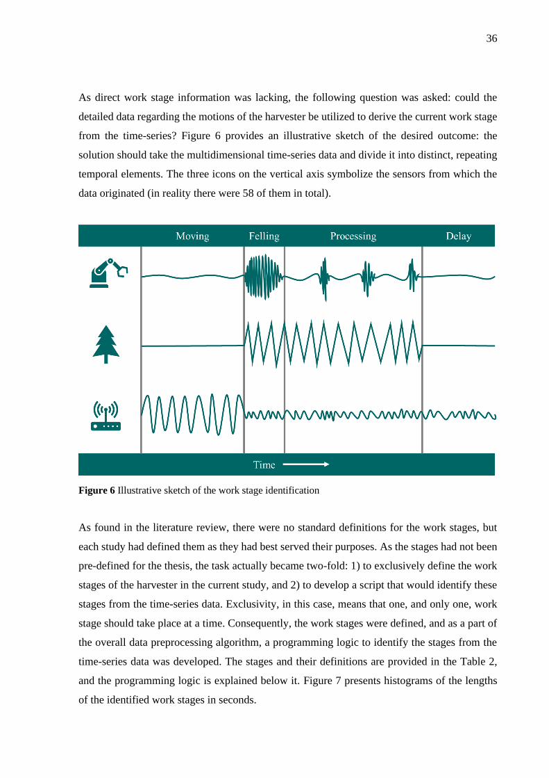
As direct work stage information was lacking, the following question was asked: could the
detailed data regarding the motions of the harvester be utilized to derive the current work stage
from the time-series? Figure 6 provides an illustrative sketch of the desired outcome: the
solution should take the multidimensional time-series data and divide it into distinct, repeating
temporal elements. The three icons on the vertical axis symbolize the sensors from which the
data originated (in reality there were 58 of them in total).
Figure 6 Illustrative sketch of the work stage identification
As found in the literature review, there were no standard definitions for the work stages, but
each study had defined them as they had best served their purposes. As the stages had not been
pre-defined for the thesis, the task actually became two-fold: 1) to exclusively define the work
stages of the harvester in the current study, and 2) to develop a script that would identify these
stages from the time-series data. Exclusivity, in this case, means that one, and only one, work
stage should take place at a time. Consequently, the work stages were defined, and as a part of
the overall data preprocessing algorithm, a programming logic to identify the stages from the
time-series data was developed. The stages and their definitions are provided in the Table 2,
and the programming logic is explained below it. Figure 7 presents histograms of the lengths
of the identified work stages in seconds.

37
Table 2 Work stage definitions used in the current study
Work stage Definition
Felling (F) Begins when the harvester head sticks to a new tree and ends when
the felling of the tree has been registered by the sensors.
Processing (P) Starts when a tree has been cut. The tree is delimbed and cross-cut
into one or more logs. Stage ends when the harvester head drops the
last log of the felled tree to the ground.
Moving (M) Driving the harvester at the site. Defined as the time when the
harvester wheels are moving.
Delays (D) When the machine is either in the idling mode or the engine is not
running at all. Delays could be for example personal breaks of the
harvester operator.
Other (O) Temporal sequences that did not fit into any of the other categories
belong to this stage. Other activities could mean e.g. crane
movements and arranging and moving logs, branches and tops.
Felling: The identification of this work stage was based on two sensor values 1)
NumberOfFellingCuts-field in the ProductionLogger-data, which indicates how many trees in
total have been cut until that point in time 2) Paksuusanturi-field (thickness sensor) in the
ArcNetReader-data in which the diameter of the tree is calculated based on the raw values
provided by the sensor. The identification started by dividing the time-series data into subsets
associated with number of felling cuts, and the idea behind was the following. When for the
last time, concerning a subset, the thickness sensor value drops below 1000, it means that the
harvester has now stuck to a new tree that will be cutted soon. The tree "is being cut" until the
end of the current subset, as being in the next subset would indicate that the number of felling
cuts has increased by one and the tree has already been cut.
Processing: Immediately after the tree has been cut (from the very beginning of the next subset
of data), starts the processing of the tree, that is, delimbing and cross-cutting the stem. Now the
harvester head is holding the stem, which is indicated by the thickness sensor value < 1000.
Stage ends when the sensor, for the first time concerning the current subset, returns to 1000
indicating that the tree has been dropped and the felling head is not processing it anymore.
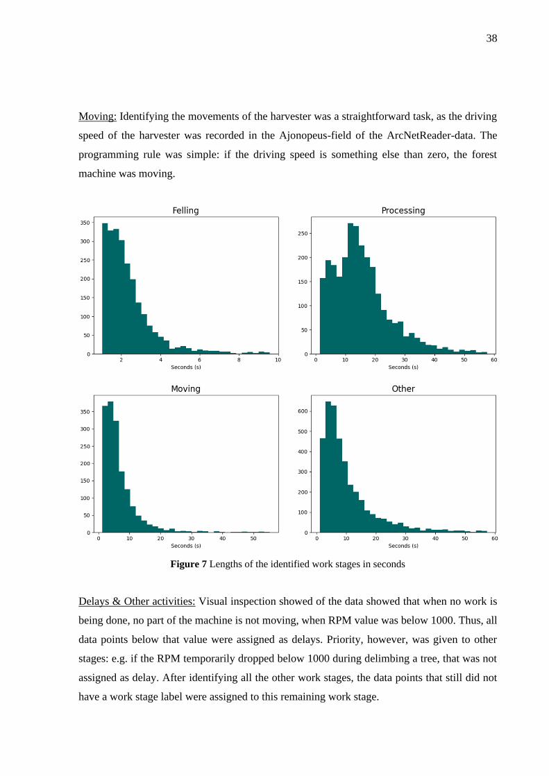
38
Moving: Identifying the movements of the harvester was a straightforward task, as the driving
speed of the harvester was recorded in the Ajonopeus-field of the ArcNetReader-data. The
programming rule was simple: if the driving speed is something else than zero, the forest
machine was moving.
Figure 7 Lengths of the identified work stages in seconds
Delays & Other activities: Visual inspection showed of the data showed that when no work is
being done, no part of the machine is not moving, when RPM value was below 1000. Thus, all
data points below that value were assigned as delays. Priority, however, was given to other
stages: e.g. if the RPM temporarily dropped below 1000 during delimbing a tree, that was not
assigned as delay. After identifying all the other work stages, the data points that still did not
have a work stage label were assigned to this remaining work stage.

39
6.4 Feature extraction
The term feature extraction was defined earlier: it means using the original data to derive a set
of new features that can be worked with the selected analytical methods. As the feature
extraction of this study was performed in highly customized manner, and as it was tightly
connected with the previous step (work stage identification) the process is further clarified by
this subchapter. Having identified the work stages, the datasets were still in time-series format,
and so far, that was not what was desired: to be able to answer the main research question of
the thesis, a matrix-form dataset, including the target variable productivity and a set of
explanatory features, whose impact on the target variable would be quantified, was required.
As harvesting productivity is defined as the volume of harvested wood per a unit of time, the
observations in the extracted dataset had to correspond to some temporal elements. Rossit et al.
(2019) had calculated a cycle time for each tree “by determining the difference between two
consecutive stem’s time stamps”. Inspired by them, the data was now divided to work cycles,
which here in this study, are defined as the temporal sequences, during which an individual tree
was felled and processed, including the possible movement from the previous tree.
Figure 8 Illustration of the division between harvester work cycles
The idea behind the division into work cycles is illustrated by Figure 8. New work cycle was
started always from the endpoint of Processing work stage (P) – from the point when the felling
head had just dropped the previous tree, and the harvester is about to head for another tree. As
the figure shows, a cycle always included at least the stages Felling (F) and Processing (P), but
it could include Other activities (O) and Moving (M) as well. Following this rule, an indicator
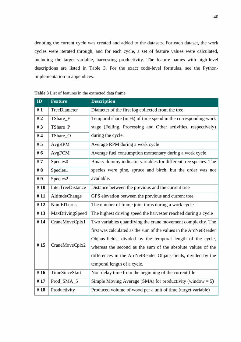
40
denoting the current cycle was created and added to the datasets. For each dataset, the work
cycles were iterated through, and for each cycle, a set of feature values were calculated,
including the target variable, harvesting productivity. The feature names with high-level
descriptions are listed in Table 3. For the exact code-level formulas, see the Python-
implementation in appendices.
Table 3 List of features in the extracted data frame
ID Feature Description
# 1 TreeDiameter Diameter of the first log collected from the tree
# 2 TShare_F Temporal share (in %) of time spend in the corresponding work
stage (Felling, Processing and Other activities, respectively)
during the cycle.
# 3 TShare_P
# 4 TShare_O
# 5 AvgRPM Average RPM during a work cycle
# 6 AvgFCM Average fuel consumption momentary during a work cycle
# 7 Species0 Binary dummy indicator variables for different tree species. The
species were pine, spruce and birch, but the order was not
available.
# 8 Species1
# 9 Species2
# 10 InterTreeDistance Distance between the previous and the current tree
# 11 AltitudeChange GPS elevation between the previous and current tree
# 12 NumFJTurns The number of frame joint turns during a work cycle
# 13 MaxDrivingSpeed The highest driving speed the harvester reached during a cycle
# 14 CraneMoveCplx1 Two variables quantifying the crane movement complexity. The
first was calculated as the sum of the values in the ArcNetReader
Ohjaus-fields, divided by the temporal length of the cycle,
whereas the second as the sum of the absolute values of the
differences in the ArcNetReader Ohjaus-fields, divided by the
temporal length of a cycle.
# 15 CraneMoveCplx2
# 16 TimeSinceStart Non-delay time from the beginning of the current file
# 17 Prod_SMA_5 Simple Moving Average (SMA) for productivity (window = 5)
# 18 Productivity Produced volume of wood per a unit of time (target variable)

41
7 REGRESSION ANALYSIS ON HARVESTER DATA
Having extracted a clean, preprocessed dataset, the task of discovering the most import factors
affecting harvesting productivity could now be represented in analytical form: which variables
in this dataset would be the most powerful predictors of the continuous target variable,
harvesting productivity? To answer the question, three different regression models were fitted.
In this chapter, the steps of that analysis, from feature selection and testing the relevant
statistical assumptions to examining the goodness-of-fit statistics, are presented. The Python-
language implementation of the analysis is provided on appendices.
7.1 Feature selection and OLS multiple regression
Being the cornerstone of regression analysis, it was the most meaningful to start the
investigation from the ordinary least-squares (OLS) model. After scaling the data into zero
mean and unit variance, an initial model with all the features was fitted. Quite as expected, as
𝑝-values of the 𝑡-test were examined, it was noticed that quite many of the 17 features would
be useless in terms of predicting the harvesting productivity. To reduce the number of redundant
predictors, automated feature selection by backward elimination (Figure 9) was conducted.
Having selected 𝛼 = 0.001 as the significance threshold, running the algorithm resulted in the
removal of six variables, 1) TShare_O 2) NumFJTurns 3) Species2 4) AvgRPM 5)
AltitudeChange and 6) TimeSinceStart, respectively, from the model.
Recall the 2nd assumption of an OLS model, given by Mellin (2006), which stated that no linear
dependencies should exist between the predictor variables. Now as the matrix of bivariate
Pearson’s correlations was examined, it was noticed that the regression model indeed suffered
from multicollinearity: high inter-correlations existed between the variables. The problem was
solved in an algorithmic manner (clarified in Figure 10): the bivariate correlations were looped
through, and always when a severe inter-correlation became apparent, that is, when the
correlation exceeded a threshold value (explained below), the feature, which had a smaller
correlation with the target variable, was removed from the model.

42
As mentioned above, the multicollinearity removal algorithm involved a threshold, which was
used as a cutoff value severe multicollinearity. The value was defined by conducting a short
literature review. According to Berry and Feldman (1985), a single number, which would be
appropriate in every situation, could not be determined, but a directive value of 0.80 was
suggested by them. Stricter thresholds were used in some studies: Donath et al. (2012), for
instance, used 0.50 as their cutoff value. That value (0.50) was then adopted to this study.
Figure 9 Backward elimination algorithm for feature selection (Modified from Srinidhi (2019))
Figure 10 Multicollinearity removal algorithm
After the process of eliminating the redundant and intercorrelated features, 10 predictors were
remaining (The process is further illustrated in Figure 11. See also Figure 12, which shows the
bivariate Pearson’s correlations after the multicollinearity was removed). Having them, the
OLS model was fitted. Table 4 lists the coefficients of the variables and several goodness-of-
fit statistics. Below, the regression results are analyzed. So far, the focus is kept solely on the
assessment of the statistical issues, whereas the answers to the research question and the
practical discussion are provided in the next chapters.

43
Figure 11 The process of eliminating the redundant and intercorrelated features
Figure 12 Heatmap of matrix of bivariate Pearson’s correlations after removing multicollinearity

44
The regression results show a number of interesting things, both promising and unsettling. First
of all, the predictive power and the accuracy of the model turned out being relatively good,
which was indicated by �̅�2 = 0.743 and 𝑀𝑆𝐸 = 0.256. A set of features, which together
explained the target variable quite well, had indeed been found. As the predictors had initially
been standardized, the magnitude of the coefficients could now be used to assess the importance
of these factors on harvesting productivity. However, before drawing more conclusions
regarding the model performance, the validity of a series of assumptions had to be studied.
Table 4 Results of OLS multiple regression
Regression results
Dep. Variable Productivity R-squared 0.744
Model OLS Adj. R-squared 0.743
Method Least Squares Mean Squared Error 0.256
No. Observations 1558 Df Model 10
Feature coef std err 𝒕 𝑷 > |𝒕| 0.025 0.975
TreeDiameter 0.7442 0.014 52.253 0.000 0.716 0.772
TShare_F 0.1317 0.014 9.665 0.000 0.105 0.158
TShare_P 0.1751 0.016 11.044 0.000 0.144 0.206
AvgFCM 0.2201 0.015 14.717 0.000 0.191 0.249
Species0 0.0786 0.014 5.484 0.000 0.050 0.107
Species1 -0.0741 0.014 -5.214 0.000 -0.102 -0.046
InterTreeDistance -0.0691 0.015 -4.592 0.000 -0.099 -0.040
MaxDriveSpeed -0.0703 0.016 -4.529 0.000 -0.101 -0.040
CraneMoveCplx2 0.0871 0.016 5.299 0.000 0.055 0.119
Prod_SMA_5 0.0618 0.013 4.678 0.000 0.036 0.088
Koenker (LMs) 200.625 Durbin-Watson 1.898
Prob(LMs) 2.45e-38 Jarque-Bera (JB) 1266.691
Skew -0.376 Prob(JB) 6.43e-20
Kurtosis 3.893 Log-Likelihood -783.36
F-statistic 903.3 Prob(F-statistic) 0.00
Koenker’s test (the robust version of Breusch-Pagan) was used to test the homoscedasticity
assumption of the regression model. The Studentized test statistic of 200.625 and the associated
𝑝-value of 2.45e-38 gave sufficient proof to reject the zero hypothesis: heteroscedasticity was
evident in the model. The non-constant residual variance was not the only flaw of the model:
the slightly bowed pattern in the scatter plot of observed versus predicted values indicated that
the linearity assumption, in this case, was not completely valid, which would cause the model
to produce erroneous results – especially if used for extrapolation purposes.

45
Durbin-Watson test was conducted to test the assumption of uncorrelated residuals. The test
statistic 𝑑 = 1.898 was compared to the table of critical values provided in the original article
(Durbin and Watson, 1951). The significance level 𝛼 = 0.05 was chosen, and sample size
𝑛 = 100 and number of predictors 𝑘 = 5 were used (as they were largest numbers for which
the critical values had been tabulated). As the values of 𝑑𝐿 and 𝑑𝑈, with the given 𝛼, 𝑛 and 𝑘,
are found between 1.57 and 1.78, respectively, the null hypothesis was not rejected, assumption
of no autocorrelation thus was being valid.
Figure 13 Scatter plot of observed vs. predicted values (left) and histogram of model residuals (right)
Jarque-Bera test was used to test the assumption of normally distributed residuals. The test
statistic 𝐽𝐵 = 1266.691, associated with 𝑝(𝐽𝐵) = 6.43e − 20, indicated that the residuals
indeed were not normally distributed. The histogram of model residuals (in Figure 13)
visualizes the finding: even though the mean of the residuals was 5.512 𝑒 − 15, which made
assuming 𝐸(𝜖𝑖) = 0 valid, there was a long tail on the positive side. With non-normal error
terms, it would be much more difficult to estimate the probability that a forecast error would
exceed a threshold in given direction.
7.2 Regression with Box-Cox transformed values
Would transforming the data help to cure the heteroscedasticity, residual distribution and non-
linear relationships within the model? That question was asked next, and after considering a
number of other transformations, such as Yeo-Johnson and the natural logarithm, the one that

46
seemed to mitigate the aforementioned problems the best was the Box-Cox transformation. By
performing the same mathematical operation (given by the equation below) on each observation
of the dataset, the transformation (Box and Cox, 1964) modifies the distributional shape of the
data in a way that it is closer to normal.
𝑦𝑖(𝜆)
= {𝑦𝑖
𝜆 − 1
𝜆𝑖𝑓 𝜆 ≠ 0
𝑙𝑛 𝑦𝑖 𝑖𝑓 𝜆 = 0
(19)
The Box-Cox transformation was applied to both explanatory features and the target. As the
transformation required the data to be strictly positive, a small shifting parameter was added to
all the variables with non-positive values. After transformation, the backward elimination and
multicollinearity removal algorithms (the same ones as with previous model) were executed
Programming-wise, this was done by implementing a function that performed both of these
steps, and the decision, whether one wanted to use standard scaling or Box-Cox transformation,
was fed as a function parameter.
Figure 14 Observed vs. predicted values and the residuals distribution after Box-Cox
Figure 14 illustrates the effects of the transformation. As the scatter plot of observed versus
predicted values shows, the points were now symmetrically distributed around a diagonal line,
indicating that the problems imposed by nonlinearity had been removed. As opposed to the
model with non-transformed values, the tail on the histogram of the error terms was now on the
negative side. The tail was also much shorter, meaning that the errors the new model had made,

47
had been smaller in magnitude. But even though the residual distribution was much closer to
normal, the problem of non-normal error terms had not fully been solved, which was indicated
by the Jarque-Bera test statistic of 88.381, associated with 𝑝(𝐽𝐵) = 6.43e − 20. To study to
effect of the transformation on heteroscedasticity, Koenker’s test was repeated. The test statistic
𝐿𝑀𝑠 = 48.084, associated with 𝑝(𝐿𝑀𝑠) = 9.523e − 8 were obtained, meaning that also the
heteroscedasticity was lessened but still existed. Table 5 presents the regression results after
Box-Cox transformation.
Table 5 Results of OLS multiple regression with Box-Cox transformed values
Regression results
Dep. Variable Productivity R-squared 0.840
Model OLS Adj. R-squared 0.839
Method Least Squares Mean Squared Error 0.160
No. Observations 1558 Df Model 9
Feature coef std err 𝒕 𝑷 > |𝒕| 0.025 0.975
TreeDiameter 0.7687 0.011 68.805 0.000 0.747 0.791
TShare_F 0.2187 0.012 18.965 0.000 0.196 0.241
TShare_P 0.1942 0.012 16.015 0.000 0.170 0.218
AvgFCM 0.1909 0.012 16.059 0.000 0.168 0.214
Species0 0.1185 0.010 11.357 0.000 0.098 0.139
InterTreeDistance -0.0514 0.012 -4.215 0.000 -0.075 -0.027
CraneMoveCplx2 0.1664 0.013 12.884 0.000 0.141 0.192
TimeSinceStart -0.0442 0.010 -4.239 0.000 -0.065 -0.024
Prod_SMA_5 0.0523 0.011 4.981 0.000 0.032 0.073
Koenker (LMs) 48.084 Durbin-Watson 1.780
Prob(LMs) 9.523e-8 Jarque-Bera (JB) 88.381
Skew -0.376 Prob(JB) 6.43e-20
Kurtosis 3.893 Log-Likelihood -783.36
F-statistic 903.3 Prob(F-statistic) 0.00
As the table shows, the Box-Cox transformation had an increasing effect on the R-squared,
which grew from 0.744 to 0.840. Correspondingly, MSE decreased from 0.256 to 0.160
indicating that the model now made smaller errors on average. Compared to the standard scaled
least-squares model, mostly the same features ended up being chosen to the final model by the
automated feature selection algorithms. The differences were the following: 1) the model no
more included variable Species1 and MaxDrivingSpeed 2) the model now included feature
TimeSinceStart, which was not present in the first model.
48
7.3 Lasso regression
After least-squares models, another approach was taken with Lasso (Least Absolute Shrinkage
and Selection Operator) regression. As discussed in Chapter 4, Lasso, by the means of adding
a penalty term to the error function, had the ability to do feature selection on high-dimensional
data. As the objective of this thesis was to discover the most important factors affecting the
harvesting productivity, Lasso seemed like a good fit: the coefficients of the features in a
regression model, which were redundant in terms of predicting harvesting productivity, would
be shrunk to zero. Higher coefficient values would then be given only to the most important
variables. Lasso had also been shown to be an effective method to mitigate the problems of
multicollinearity, which indeed was the case in the current dataset. Here, it was desired that
Lasso would shrink the coefficients of the predictors causing the strong interdependencies.
To implement the Lasso model, GridSearchCV-function was used in Python. The term “grid
search” in the function name refers to the strategy using which the penalty parameter 𝜆 was
selected: by an exhaustive search over a set of options. As Bergstra and Bengio (2012) point
out: optimizing model hyper-parameters like this typically results in better solutions than
manual selection, but especially when used in large number of dimensions, the method can be
exceedingly time-consuming. Abbreviation “CV”, on the other hand, stands for cross-
validation. The main idea of 𝑘-fold cross-validation is explained well by Refaeilzadeh et al.
(2009): after dividing the data into 𝑘 folds (aka segments) of equal size, 𝑘 iterations are
performed in a way that 𝑘 − 1 of these folds are always used training, whereas the remaining
segment of data is used for testing. Having completed the iteration rounds, simple averaging
can be used to obtain an aggregate measure from these sample, but alternative techniques exist
as well. In this analysis, 5-fold cross-validation was used, which was the default setting in the
GridSearchCV-function and which is known to be a common practice in data mining.
Lasso was fitted to the scaled (zero mean and unit variance) data. All 17 variables were
included, and as Lasso itself was now the feature selection method, the workflow this time did
not include feature selection of any other type (like backward selection that was done with
OLS). The results of the model, the coefficients and selected goodness-of-fit statistic, are
provided in Table 6. According to the grid search algorithm, the optimal penalty parameter

49
lambda (the one that produced the highest coefficient of determination) was 𝜆 = 0.01. The
values 𝑅2 = 0.772 and 𝑀𝑆𝐸 = 0.253 were slightly better but equal magnitude to the values
obtained with least-squares method and standard scaling. The features that had the highest
impact on the regression model were TreeDiameter, TShare_F, TShare_P, AvgFCM,
CraneMoveCplx2 and Prod_SMA_5 with coefficient 0.727, 0.117, 0.161, 0.229, 0.093 and
0.056, respectively Moreover, especially the features Species1, InterTreeDistance, and
MaxDriveSpeed had a notable effect in the model. The coefficients of the variables that were
not mentioned above were shrunk either to zero or to some very small value.
Table 6 Coefficients in Lasso regression
Regression results
Dep. Variable Productivity R-squared 0.772
Method Lasso MSE 0.253
No. Observations 1558 Lambda λ 0.01
Coefficients
TreeDiameter 0.727 Species0 0.069 MaxDriveSpeed -0.073
TShare_F 0.117 Species1 -0.064 CraneMoveCplx1 -0.031
TShare_P 0.161 Species2 -0.000 CraneMoveCplx2 0.093
TShare_O -0.001 InterTreeDistance -0.067 TimeSinceStart -0.017
AvgRPM 0.009 AltitudeChange 0.022 Prod_SMA_5 0.056
AvgFCM 0.229 NumFJTurns -0.000
Koenker (LMs) 219.609 Jarque-Bera (JB) 1532.257
Prob(LMs) 0.000 Prob(JB) 0.000
Even though the estimation method in Lasso is different from OLS, and the least-squares
assumptions are not directly applicable to Lasso estimation, it is important to remember that
both methods are used to estimate a linear regression model. In the current case, there is no
evidence that Lasso estimation would had substantially increased the validity of one of the main
assumptions in linear regression: the target variable being linearly dependent on the explanatory
features. Plotting the observed vs. predicted values produced almost identical pattern to the one
that was seen in Figure 13 with OLS estimation. Moreover, Koenker's test statistic 𝐿𝑀𝑆 =
219.609, which corresponded to 𝑝(𝐿𝑀) close to zero, showed that heteroscedasticity existed
also in the Lasso-estimated model, and the Jarque-Bera test statistic 1532.257, associated with
𝑝-value close to zero, gave a proof that neither the problem of non-normally distributed
residuals was removed.

50
8 EMPIRICAL RESULTS
Based on the data at hand, what are the most important factors affecting harvesting
productivity? Now, having considered three different regression models, it was finally possible
to answer the main research question of the thesis. But having obtained the standardized
coefficients of different 17 features, which ones were the most important? This rather
ambiguous and qualitative expression was converted into a straightforward rule: the most
important factors were the ones that had a non-zero coefficient in all three models, that is, all
three models had considered them as statistically significant. Using that rule, a set of eight
important factors were found, and they are visualized in the clustered bar chart in Figure 15.
The chart shows the coefficients of the variables and the differences between the three models
1) OLS regression with standard scaling, 2) OLS with Box-Cox transformation and 3) Lasso
regression. Below the figure, the findings analyzed and interpreted.
Figure 15 The most important variables affecting harvesting productivity
According the results, the most important variable affecting harvesting productivity is the
diameter of the felled tree (coefficients from 0.73 to 0.77). As the productivity of a harvesting
work cycle was defined as the volume of collected wood divided by the elapsed time – and as

51
the diameter of a tree is a direct estimator of the stem volume – the causality is evident:
harvesting productivity is increased the best by cutting thick trees instead of the thinner ones.
When it comes to the magnitudes of the coefficients, the seven other factors – as one notices
from the chart – were far behind. Moreover, the causal relationships with the target variable
were less obvious. Going from left to right, the next two factors, TShare_F and TShare_P
(coefficients from 0.12 to 0.22), denoted the temporal shares of a work cycle spend in felling
and processing, respectively. The result can be interpreted as follows: when a high percentage
of time has been spent in felling and processing, less time has been spent in non-value-adding
work, such as moving and other activities. However, by common sense one comprehends that
the causality is not fully direct: harvesting productivity does not increase by felling, delimbing
and cross-cutting the trees slower, but by reducing the time spent in activities other than that.
The fourth factor AvgFCM (coefficients from 0.19 to 0.23) stood for the average fuel
consumption momentary: the bigger the value, the faster the fuel had been consumed during
the harvesting work. But again the causality cannot be considered as direct: it is not meaningful
to say that the harvesting productivity would increase by consuming the fuel faster. Instead, the
result can be interpreted as follows: when the fuel consumption has been high, the harvester
might have been operated in more active and effective manner, that is, less idle time has
occurred, which has then led to higher productivity. In other words, the harvester has been
performing its core work (felling and processing the trees) more continuously, which had
consumed more fuel on average than the stand-by mode.
Corresponding to the fifth factor, a small but notable effect on harvesting productivity
(coefficients from 0.07 to 0.12) seems to be associated with the species of the felled tree. The
cause-and-effect relationship, however, is questionable also in this case: it is not very likely that
it would be the tree species itself that led the harvester to cut wood faster. More likely
explanation would be the tendency of one species to grow bigger than the others: when the
harvester had focused on felling that particular species, it had statistically been more productive.
The metadata for this study did not include a clear mapping from the numerical species
indicators to the species names, but presumably, this “biggest” tree species is pine.

52
The sixth factor, inter-tree distance, seems to have a negative effect on harvesting productivity.
The finding is rather intuitive: the farther apart the trees are from each other, the more the
harvester has to move between them, making the fellings less productive. However, it is
important to notice here that the distances between the trees have been calculated from the GPS
locations of the harvester, not from the actual trees (nor the harvester crane). Also, as the crane
has maximum reach of 10-11 meters, multiple trees (instead of just one tree) can be felled
during a moment of standing (that is, the harvester does not have to move after felling each
tree). Therefore, instead of suggesting keeping the distances short, the finding can actually be
interpreted as a support for moving the harvester itself less frequently.
The idea of the seventh factor CraneMoveCplx2 (coefficients from 0.09 to 0.17) was to quantify
how complex the movements of the crane have been during the work cycle. The value of the
variable was calculated as a sum of the absolute values of the differences in the ArcNetReader
Ohjaus-fields, divided by the temporal length of the work cycle. The meaning, in simple
English, could be summarized as follows: the higher the value, the more rapidly the operator
been pressing the crane control buttons, which has then caused the crane to move in more
complex ways. One of the latent factors (let it be sought from afar) of this variable might
actually be the skill level of the operator. The data was collected from fellings performed both
by experienced professionals and less experienced vocational students. The possible
explanation would then be that the experienced professionals, who have mastered the art of
operating the machine, that is, “pulling the right harvester levers at a right rime”, have
controlled the machine more skillfully and efficiently, which has led to higher productivity.
The rightmost bar in the chart (Prod_SMA_5) denotes the moving average of the productivity
of previous five cycles (excluding the current one). With coefficients from 0.05 to 0.06, it seems
that the productivity of the preceding cycles indeed affects the productivity of the current cycle.
Note that the choice of using five previous cycles was rather arbitrary: if 10 or 20 last cycles,
for example, were used, the result might have differed from the ones obtained in the current
case. To interpret the result, one might first think of similar explanation than with inter-tree
distance, that is, to associate it with the frequency the harvester had to move. That interpretation,
however, is made questionable by the fact that these two factors are almost perfectly
uncorrelated (Pearson’s coefficient = 0.01). Another explanation, perhaps a better one, is the

53
continuity of the work: when consecutive cycles have been productive, it means that the felling
work has taken place uninterruptedly, which has caused less time to be spent, for instance,
idling of the machine.
Let us also discuss two factors which did not seem to affect harvesting productivity. The first
one of them is altitude change, which was calculated as the differences of the altitudes given
by the GPS between the current and the previous work cycle. Before regression analysis, it was
expected that the variable would have an effect to productivity even to some extent, but
interestingly, it did not. First, there are concerns regarding the accuracy of the GPS elevation
readings, which are generally known to be much less accurate than the latitude/longitude
readings. If one would like to reliably study the effect of altitude change on harvesting
productivity, one should be able to register already the small changes in the elevation. Another
explanation to the result might be the flatness of the terrain in Mikkeli and Pieksämäki: the sites
contained so little altitude differences that they did not have any effect on harvesting. But it is
also good to notice the enormous size of the Ponsse Scorpion harvester: even a bit hillier forest
would not have had much effect on its work.
The factor TimeSinceStart was brought into the investigation to study the following question:
could the operator, after several hours of work, get tired in a way that it had a significant effect
on productivity? The idea does not sound too far-fetched when one considers the temporal
lengths of the fellings: the largest csv-file with 1.8 million observations corresponded to little
bit over 10 hours of work. As the factor, in this case, did not seem to have any impact on the
productivity, one could conclude that an operator is able to perform the work just as efficiently
right after starting and just before finishing a work shift (of course, breaks have been taken, as
the log file indicated). The finding, however, is based on an assumption that the same person
has been operating the harvester all the time, which is known to be not true. The possible
changes of shift were not registered in the current data, but it is known that the changes have
occasionally taken place during the fellings.
54
9 DISCUSSION
All the steps of the data mining process, from data collection and preprocessing to fitting the
analytical models and interpreting the results, have now been gone through. Before wrapping
up the study in a form of a summary, the following two questions are discussed: Why were
certain methods used in this thesis and what does it mean from the from the point of view of its
results? How does this study contribute to science and what would be the most meaningful
directions of further research?
9.1 On the methods and results
In this thesis, a set of factors affecting the harvesting productivity were proposed based on the
coefficients of three different linear regression models. But why linear regression? Why not
some more sophisticated model, such as neural network or support vector regression? Shortly:
because linear regression was seen to be serving the practical purpose of this thesis the best.
Instead of building an actual predictive model that could be used to forecast new values as
accurately as possible, the objective was an explorative one: to discover the factors affecting
harvesting productivity. Naturally, there is a myriad of advanced models, both regression and
non-regression, which could have been used to get a better fit with the data at hand, but the
standardized coefficients of linear regression, in this case, were seen to provide the most useful
and explainable way to assess the importance of the individual variables in predicting the
continuous target variable.
When the analytical methods for this study were selected, the most considerable challenger to
regressions were the decision trees. In the study of Rossit et al. (2019) A Big Data approach to
forestry harvesting productivity, decision trees were used to assess how different variables
affect the productivity of a harvester. The major advantage of decision trees in their case was
the interpretability: decision tree broke the complicated process of decision-making into a series
of simple rules, and the most important variables were indicated by their location in the
beginning of the tree. But as the categorization of the continuous target variable into a number
of discrete bins, which was performed in their study, was found rather artificial and arbitrary
(at least from the point of view of this study), decision trees were not used in this thesis.

55
To justify the modeling choices here, also the highly customized data preprocessing methods,
used in this study, have to be considered. The dataset for the regression analysis was certainly
not taken for granted, but it was actually built within this study: near to three gigabytes of data
in multiple csv-files, corresponding to ten million time-series observations, were compressed
into single dataset of couple hundred kilobytes using methods that were self-tailored for the
purposes of this study. But despite the fact that the data preprocessing might have had a couple
more twists than usually, let us continue this discussion as if the regression analysis were fitted
to data that validated completely. Having said that, the choices now need some further
reasoning, because statistically speaking OLS was not quite the optimal model for the data.
Recall six standard assumptions (Mellin, 2006) that were presented in the theoretical part of
this thesis. Fulfilling those assumptions would indicate that least squares is the best linear
unbiased estimator and no other estimators are needed (Brooks, 2014). Fitting the OLS model
then showed that only some of those assumptions were met with the harvester data. Even though
Box-Cox transformation successfully solved the problem with non-linear dependencies,
multicollinearity and heteroscedasticity, for instance, still remained in the model. Why was
OLS still used instead of some other models, which could have dealt better with the
abovementioned issues?
Let us start with multicollinearity. The problem, of course, was alleviated by the algorithmic
multicollinearity removal solution, but only to a certain extent: as a threshold of 0.50 was used,
correlations up to that value still remained. A question arises: should principal component
regression have been used to remove multicollinearity from the data? The answer is yes – if
one’s purpose was to build an actual predictive model and one wanted to ensure that no inter-
dependencies exist between the predictors. But would it have helped in the practical task of
discovering the factors affecting harvesting productivity. The answer is no. Instead, having a
set of linearly independent but uninterpretable principal components would have made it much
more difficult to assess the importance of individual variables. There are also models, such
quantile regression, that could have been used to handle heteroscedasticity. But again to remind:
the aim here was not to forecast any new values, and with that, taking the non-constant residual
variance into account was not absolutely necessary.

56
Then, what about the numerical values of the coefficients? Can one say that a certain factor is
more important than another based on the magnitudes of the coefficients? Should one interpret
them, for instance, in a way that 𝑥-% of increase in certain variable corresponds to 𝑦-% increase
in productivity? When the whole data mining pipeline considered, with the complex data
preprocessing and regression analysis, which involved a number of compromises, one cannot
say that the precise, numeric values regarding the magnitude of effect would be very reliable.
Instead, the results here (alongside with the cause-effect relationships that were analyzed in
previous chapter) should be taken as a useful rule of thumb: the direction is right, and the
magnitudes of the coefficients provide a rough and approximate order of importance.
9.2 Scientific contributions and suggested directions of further research
As discussed in the literature review, several studies in forest machinery productivity had used
the concept of harvester work stages to divide the workflow of a harvester into the key actions
from which it typically constituted of. On those cases, the information regarding the current
stage had always been collected by a human observer, but the data for this study did not include
that kind of field. To the current best knowledge of the author himself, this thesis is the first one
to present a programmatic way to identify the work stages of a harvester from these type of
multidimensional time-series data. Identifying the stages using the proposed programmatic
solution made it possible to study the factors affecting the harvesting productivity in a unique
way, and hence, to contribute to the scientific discussion. For instance, the temporal shares of
felling, delimbing and cross-cutting were found to be among the most important factors
affecting harvesting productivity. The results also further establish the general conclusion that
the most important factor affecting harvesting productivity is the average volume of the felled
individuals (which in this study was represented by the variable TreeDiameter). For instance,
Rossit et al. (2019), Lee et al. (2019), Eriksson and Lindroos (2014) and Rodrigues et al. (2019)
had come to the similar conclusion.
But what if one compared the most important factors affecting harvesting productivity in boom-
corridor thinning (BCT) versus selective harvesting? Would there be differences? As previous
research has shown BCT to be much more productive method than conventional thinning, one
could also examine the productivity in general: how large would the difference in productivities

57
be, based on these current data? These interesting directions for future research would be
offered if data the data included an indicator that separated between the thinning methods. In
other words, some kind of flag that told the analyst whether the current dataset corresponds to
boom-corridor thinning or selective thinning would be needed. With that, a similar study to the
current one could be conducted to discover the differences. However, as the harvester data
collection systems (according to the authors own understanding) are unable to automatically
separate the thinning methods from each other, a human person would presumably be required
to manually collect these information.
Another interesting question for further investigation – which takes the idea of work stage
identification a little further – is the following: what kind of results would we get if the stages
were not identified by a fixed programming logic (as in the current case), but with unsupervised
machine learning? Concretely, one could try a new method, Toeplitz Inverse Covariance-Based
Clustering (Hallac et al., 2017), to discover repeated temporal patterns in the data. The method
has already been used to find stages from a time-series data collected from cars (steering,
braking, accelerating, etc.), and the clustering results have corresponded the real-world, human-
interpretable actions astonishingly well. The algorithm, however, is known to be
computationally very demanding. Given the size of the data in the current study, careful data
preprocessing and possibly some advanced computing resources, such as supercomputer, would
probably be needed to make the algorithm converge in a reasonable time.

58
10 SUMMARY AND CONCLUSIONS
The topic for this thesis arose from PUUSTI research project aiming to study and demonstrate
a new harvesting technique, boom-corridor thinning (BCT). A series of fellings were conducted
in South-Eastern Finland during May-October 2020 using Ponsse Oy’s harvesters, and a set of
multidimensional sensor data were collected from them using a data collection software
developed by Creanex Oy. As the data consisted of 9.6 million time-series observations, which
had been collected from 58 sensors in 0.02 second intervals, the material for the study
corresponded to over 53 hours of harvesting work, during which more than 2,6 thousand trees
had been felled. Having these data, the following question was asked: how could they be
utilized in order to examine and/or develop harvesting productivity? After consideration of a
number of utilization possibilities, the specific research questions, which turned out being both
feasible and the most meaningful to be answered, were the following:
1. Based on these data, what are the factors affecting harvesting productivity?
2. Which work stages can be identified from these harvester data and how?
Answering the questions began by conducting a systematic literature review. One of its main
findings was that harvesting productivity is affected by several factors. The one that is generally
considered as the most important is the stem size (the average volume of wood a felled
individual contains), but many other factors explain the productivity as well: stand density, tree
species, experience level of the operator, work shift, terrain, road spacing and condition,
weather and other seasonal conditions, forwarder load capacity as well as the technical
capability of the harvester, to name a few. Another key finding was that the harvester work
stages did not have any standardized definitions in scientific literature: despite more or less
similar stages being involved in most of the studies, different ways to distinguish between the
stages had been used by different researchers. The theoretical part of the thesis also introduced
the reader into the concept and process of data mining as well as provided a selection of theory
on regression analysis.
The empirical part of the thesis then presented a complete data mining pipeline to determine
the most important factors affecting harvesting productivity from the harvester data. Using

59
Python programming language, a comprehensive data preprocessing and feature extraction
algorithm was developed for these data. The algorithm took the raw csv-files, used the sensor
information on the harvester motions to identify five work stages (felling, processing, moving,
delays and other activities) from the time-series data, and simultaneously, by extracting a set of
17 explanatory variables, gradually built a data frame, in which the rows corresponded to the
temporal sequences, during which an individual tree had been felled and processed (including
possible movement from the previous tree).
To determine the most important factors affecting harvesting productivity, regression analysis
was then conducted on this preprocessed dataset. Firstly, after an automated feature selection
with backward elimination, OLS multiple regression was fitted both with standardized (𝜇 = 0
and 𝜎2 = 1) and Box-Cox-transformed values. R-squared values of 0.74 and 0.84, respectively,
were obtained for these two models, and their validities were studied with selected statistical
tests, including Koenker, Durbin-Watson and Jarque–Bera tests. Also, Lasso regression, with
grid-search cross-validation based optimization of the penalty parameter λ, was fitted, and this
time R-squared value of 0.77 was obtained. Finally, the most important factors affecting
harvesting productivity were obtained by choosing the ones that had been considered
statistically significant by all three regression models.
As a result of this thesis, eight factors affecting harvesting productivity were discovered,
including the diameter of the felled tree, the temporal shares of felling and processing (i.e.
delimbing and cross-cutting) from the total work time, average fuel consumption, tree species,
inter-tree distance, crane movement complexity and the moving average of the harvesting
productivity. By far the most important factor (with standardized coefficients from 0.73 to 0.77)
was the tree diameter, as opposed to the other seven factors with coefficients from 0.05 up to
0.23. The factors that did not seem to affect the productivity include, for instance, the altitude
changes, the driving speed between the trees and the time since starting the current fellings.

60
REFERENCES
Aggarwal, C.C. 2015. Data Mining: The Textbook. Springer.
Ahlemeyer‐Stubbe, A., Coleman, S. 2014. A Practical Guide to Data Mining for Business and
Industry, 1st edition. Wiley.
Ahnlund Ulvcrona, K., Bergström, D., Bergsten, U. 2017. Stand structure after thinning in 1–
2 m wide corridors in young dense stands. Silva Fennica, vol. 51, no. 3.
Baltagi, B.H. 2011. Econometrics, 5th edition. Springer.
Bergstra, J., Bengio, Y. 2012. Random Search for Hyper-Parameter Optimization. Journal of
Machine Learning Research, vol. 13, pp. 281–305.
Bergström, D., Bergsten, U., Nordfjell, T. 2010. Comparison of Boom-Corridor Thinning and
Thinning From Below Harvesting Methods in Young Dense Scots Pine Stands. Silva Fennica,
vol. 44, no. 4, pp. 669–679.
Bergström, D., Bergsten, U., Nordfjell, T., Lundmark, T. 2007. Simulation of Geometric
Thinning Systems and Their Time Requirements for Young Forests. Silva Fennica, vol. 41, no.
1, pp. 137–147.
Berkson, J. (1944). Application of the Logistic Function to Bio-Assay. Journal of the American
Statistical Association, vol. 39, no. 227, pp. 357–365.
Berry, W.D., Feldman, S. 1985. Multiple Regression in Practice, 1st edition. Quantitative
Applications in the Social Sciences. SAGE Publications.
Box, G.E.P., Cox, D.R. 1964. An Analysis of Transformations. Journal of the Royal Statistical
Society, vol. 26, no. 2. Series B (Methodological), pp. 211–252.
Breusch, T.S., Pagan, A.R. 1980. The Lagrange Multiplier Test and its Applications to Model
Specification in Econometrics. The Review of Economic Studies, vol 47, no. 1, pp. 239–253.

61
Breusch, T.S., Pagan, A.R., 1979. A Simple Test for Heteroscedasticity and Random Coefficient
Variation. Econometrica, vol 47, no. 5, pp. 1287–1294.
Brooks, C. 2014. Introductory Econometrics for Finance, 3rd edition. Cambridge University
Press.
Bühlmann, P., van de Geer, S. 2011. Statistics for High-Dimensional Data, Springer Series in
Statistics. Springer.
Cambridge Dictionary. 2020. Cambridge English Dictionary: Meanings & Definitions [WWW
Document]. Available: https://dictionary.cambridge.org/dictionary/english. Accessed
10.11.2020.
Chai, T., Draxler, R.R. 2014. Root mean square error (RMSE) or mean absolute error (MAE)?
– Arguments against avoiding RMSE in the literature. Geoscientific Model Development, vol.
7, no. 3, pp. 1247–1250.
Chakrabarti, S., Ester, M., Fayyad, U., Gehrke, J., Han, J., Morishita, S., Piatetsky-Shapiro, G.,
Wang, W. 2006. Data Mining Curriculum: A Proposal (Version 1.0). ACM SIGKDD
Curriculum Committee.
Corte, A., Sanquetta, C., Wojciechowski, J., Rodrigues, A., Maas, G. 2013. On the use of data
mining for estimating carbon storage in the trees. Carbon Balance and Management, vol. 8, no.
6.
Cortes, C., Vapnik, V. 1995. Support-vector networks. Machine Learning, vol. 20, pp. 273–
297.
Defays, D. 1977. An efficient algorithm for a complete-link method. The Computer Journal, vol.
20, no. 4, pp. 364–366.
Di Fulvio, F., Bergström, D., Kons, K., Nordfjell, T. 2012. Productivity and Profitability of
Forest Machines in the Harvesting of Normal and Overgrown Willow Plantations. Croatian
Journal of Forest Engineering, vol. 33, no. 1, pp. 25–37.

62
Domingos, P., Pazzani, M. 1997. On the Optimality of the Simple Bayesian Classifier under
Zero-One Loss. Machine Learning, vol. 29, pp. 103–130.
Donath, C., Gräßel, E., Baier, D., Pfeiffer, C., Bleich, S., Hillemacher, T. 2012. Predictors of
binge drinking in adolescents: Ultimate and distal factors - A representative study. BMC Public
Health.
Dormann, C.F., Elith, J., Bacher, S., Buchmann, C., Carl, G., Carré, G., Marquéz, J.R.G.,
Gruber, B., Lafourcade, B., Leitão, P.J., Münkemüller, T., McClean, C., Osborne, P.E.,
Reineking, B., Schröder, B., Skidmore, A.K., Zurell, D., Lautenbach, S. 2012. Collinearity: a
review of methods to deal with it and a simulation study evaluating their performance.
Ecography, vol. 36, no. 1, pp. 27–46.
Durbin, J., Watson, G.S. 1951. Testing for Serial Correlation in Least Squares Regression: II.
Biometrika, vol. 38, no. 3/4, pp. 409–428.
Durbin, J., Watson, G.S. 1950. Testing for Serial Correlation in Least Squares Regression: I.
Biometrika, vol. 37, no. 1/2, pp. 159–177.
Erber, G., Holzleitner, F., Kastner, M., Stampfer, K. 2016. Effect of multi-tree handling and
tree-size on harvester performance in small-diameter hardwood thinnings. Silva Fennica, vol.
50, no. 1.
Eriksson, M., Lindroos, O. 2014. Productivity of harvesters and forwarders in CTL operations
in Northern Sweden based on large follow-up datasets. International Journal of Forest
Engineering, vol. 25, no. 3, pp. 179–200.
Ester, M., Kriegel, H-P., Sander, J., Xiaowei, X. 1996. A density-based algorithm for
discovering clusters in large spatial databases with noise. Proceedings of the Second
International Conference on Knowledge Discovery and Data Mining (KDD-96).
Everitt, B.S., Skrondal, A. 2010. The Cambridge Dictionary of Statistics, 4th edition. Cambridge
University Press.
Famili, A., Shen, W.-M., Weber, R., Simoudis, E. 1997. Data Preprocessing and Intelligent
Data Analysis. Intelligent Data Analysis Journal, vol. 1, no. 1, pp. 3–23.

63
Fayyad, U., Piatetsky-Shapiro, G., Smyth, P. 1996. From Data Mining to Knowledge Discovery
in Databases. AI Magazine. American Association for Artificial Intelligence.
Fernandez-Granda, C. 2017. Probability and Statistics for Data Science. New York University.
García, S., Ramírez-Gallego, S., Luengo, J., Benítez, J.M., Herrera, F. 2016. Big data
preprocessing: methods and prospects. Big Data Analytics, vol. 1, no. 1.
Google, 2020. Google Maps [WWW Document]. Available: https://www.google.fi/maps/.
Accessed 10.10.2020.
Greasley, A. 2019. Simulating Business Processes for Descriptive, Predictive, and Prescriptive
Analytics. Walter de Gruyter GmbH & Co KG.
Hallac, D., Vare, S., Boyd, S., Leskovec, J. 2017. Toeplitz Inverse Covariance-Based
Clustering of Multivariate Time Series Data. Proceedings of the 23rd ACM SIGKDD
International Conference on Knowledge Discovery and Data Mining.
Han, J., Kamber, M., Pei, J. 2012. Data Mining. Concepts and Techniques, 3rd edition. The
Morgan Kaufmann Series in Data Management Systems. Elsevier.
Hearst, M.A. 1999. Untangling text data mining. Proceedings of the 37th annual meeting of the
Association for Computational Linguistics on Computational Linguistics (ACL '99), pp. 3–10.
Hoerl, A.E., Kennard, R.W. 1970. Ridge Regression: Biased Estimation for Nonorthogonal
Problems. Technometrics, vol. 12, no. 1, pp. 55–67.
Jarque, C.M., Bera, A.K. 1987. A Test for Normality of Observations and Regression Residuals.
International Statistical Review, vol. 55, no. 2, pp. 163–172.
Kaplan, A., 2004. A Beginner’s Guide to Partial Least Squares Analysis. Understanding
Statistics, vol. 3, no. 4.
Kärhä, K., Jouhiaho, A., Mutikainen, A., Mattila, S. 2013. Mechanized Energy Wood
Harvesting from Early Thinnings. International Journal of Forest Engineering, vol. 16, no. 1,
pp. 15–25.

64
Kaur, M., Kang, S. 2016. Market Basket Analysis: Identify the Changing Trends of Market Data
Using Association Rule Mining. Procedia Computer Science, vol 85, pp. 78–85.
Koenker, R. 1981. A note on studentizing a test for heteroskedasticity. Journal of Econometrics,
vol. 17, no. 1, pp. 107–112.
Kyriakidis, I., Kukkonen, J., Karatzas, K., Papadourakis, G., Ware, A. 2015. New Statistical
Indices for Evaluating Model Forecasting Performance. New Horizons in Industry, Business
and Education.
Lane, D.M., Scott, D., Hebl, M., Guerra, R., Osherson, D., Zimmer, H. 2003. Introduction to
Statistics: Online edition. Rice University.
Langin, D., Ackerman, P., Benno, K., Immelmann, A., Potgieter, C., van Rooyen, J. 2010. South
African ground based harvesting handbook, 1st edition. FESA.
Lee, E., Han, S.-K., Im, S. 2019. Performance Analysis of Log Extraction by a Small Shovel
Operation in Steep Forests of South Korea. Forests, vol. 10.
Lyon, J.D., Tsai, C.-L. 1996. A Comparison of Tests for Heteroscedasticity. Journal of the
Royal Statistical Society, Series D (The Statistician), vol. 45, no. 3, pp. 337–349.
MacQueen, J. 1967. Some methods for classification and analysis of multivariate observations.
University of California Press. Proceedings of the Fifth Berkeley Symposium on Mathematical
Statistics and Probability, vol. 1, pp. 281–297.
Mai, C., Reddy, A., Muralikrishna, I. 2004. Polyanalyst Application for Forest Data Mining.
IEEE Conference IGARSS.
Mellin, I. 2006. Tilastolliset menetelmät: Lineaarinen regressioanalyysi. Teknillinen
korkeakoulu.
Mohammadi, J., Shataee, S., Babanezhad, M. 2011. Estimation of forest stand volume, tree
density and biodiversity using Landsat ETM+ Data, comparison of linear and regression tree
analyses. 1st Conference on Spatial Statistics.
Motoda, H., Liu, H., 2002. Feature Selection, Extraction and Construction.

65
Mousavi Mirkala, S.R. 2009. Comparison of productivity, cost and environmental impacts of
two harvesting methods in Northern Iran: short-log vs. long-log. Dissertationes Forestales, vol.
82.
Nakagawa, M., Hayashi, N., Narushima, T. 2010. Effect of tree size on time of each work
element and processing productivity using an excavator-based single-grip harvester or
processor at a landing. Journal of Forest Research, vol. 15, no. 4, pp. 226–233.
Northern Illinois University, 2005. Responsible Conduct in Data Management: Data Collection
[WWW Document]. Available:
ori.hhs.gov/education/products/n_illinois_u/datamanagement/dctopic.html. Accessed
10.11.2020.
Nuutinen, Y., Väätäinen, K., Heinonen, J., Asikainen, A., Röser, D. 2008. The accuracy of
manually recorded time study data for harvester operation shown via simulator screen. Silva
Fennica, vol. 42, no. 1, pp. 63–72.
Olivera, A. 2016. Exploring opportunities for the integration of GNSS with forest harvester
data to improve forest management. Doctoral dissertation in University of Canterbury.
Özbayoglu, M., Bozer, R. 2012. Estimation of the Burned Area in Forest Fires Using
Computational Intelligence Techniques. Procedia Computer Science, vol 12, pp. 282–287.
Ponsse Oyj. 2020. Company website [WWW Document]. Available: www.ponsse.com.
Accessed 7.13.2020.
Purfürst, T., Erler, J. 2011. The human influence on productivity in harvester operations.
International Journal of Forest Engineering, vol. 22, no. 2, pp. 15–22.
Pyle, D. 1999. Data Preparation for Data Mining. Morgan Kaufmann Publishers, Inc.
Quinlan, J.R. 1986. Induction of decision trees. Machine Learning, vol 1, pp. 81–106.
Räsänen, T. 2018. The potential and use principles of harvester production data as forest
resource information. NB-NORD Workshop on Big Data from Forest Machines.

66
Refaeilzadeh, P., Tang, L., Huan, L. 2009. Cross-Validation. Encyclopedia of Database
Systems. Springer.
Rodrigues, C.K., Lopes, E. da S., Pereira, A.L.N., Sampietro, J.A. 2019. Effect of individual
tree volume on operational performance of harvester processor. Floresta, vol. 49, no. 2, pp.
345–352.
Rossit, D.A., Olivera, A., Viana Céspedes, V., Broz, D. 2019. A Big Data approach to forestry
harvesting productivity. Computers and Electronics in Agriculture, vol. 161, pp. 29–52.
Rossit, D.A., Viana Céspedes, A., Broz, D. 2017. Application of data mining to forest
operations planning. Big DSS Agro.
Sammut, C., Webb, G.I. 2017. Encyclopedia of Machine Learning and Data Mining, 2nd
edition. Springer.
Saukkola, A., Melkas, T., Riekki, K., Sirparanta, S., Peuhkurinen, J., Holopainen, M., Hyyppä,
J., Vastaranta, M. 2019. Predicting Forest Inventory Attributes Using Airborne Laser Scanning,
Aerial Imagery, and Harvester Data. Remote Sensing, vol. 11, no. 7.
Sondhi, P. 2009. Feature Construction Methods: A Survey. University of Illinois at Urbana
Champaign.
Srinidhi, S. 2019. Backward Elimination for Feature Selection in Machine Learning [WWW
Document]. Available: https://towardsdatascience.com/backward-elimination-for-feature-
selection-in-machine-learning-c6a3a8f8cef4. Accessed 27.10.2020.
Taylor, D. 2007. A Brief Guide To Writing A Literature Review [WWW Document]. University
of Toronto. Available:
https://journals.scholarsportal.info/pdf/19207093/v01i0001/12_abgtwalr.xml. Accessed
27.10.2020.
Tibshirani, R. 1996. Regression Shrinkage and Selection via the Lasso. Journal of the Royal
Statistical Society, vol. 58, no. 1, pp. 267–288.

67
Webster, J., Watson, R.T. 2002. Guest Editorial: Analyzing the Past to Prepare for the Future:
Writing a literature Review. MIS Quarterly, vol. 26, no. 2, pp. 13–23.
Xanthopoulos, P., Pardalos, P.M., Trafalis, T.B. 2013. Robust Data Mining, SpringerBriefs in
Optimization. Springer.
Yazdani, M., Jouibary, S.S., Mohammadi, J., Maghsoudi, J. 2020. Comparison of different
machine learning and regression methods for estimation and mapping of forest stand attributes
using ALOS/ PALSAR data in complex Hyrcanian forests. Journal of Applied Remote Sensing,
vol. 14, no. 2.

68
APPENDICES
A1 Metadata of the collected harvester log files
COLUMN DESCRIPTION
Time Time in seconds from the beginning of the current file. The
interval is 20 milliseconds.
ArcNetReader OhjausKaanto- Turning the crane to the left. The fields starting with
“ArcNetReader Ohjaus…”, denote the current value (mA) of
the control of the proportional valve of the hydraulic
movement. The minimum and maximum values have been
adjusted in the control system: currently they vary between
the 0 mA and ≈500 mA.
ArcNetReader OhjausKaanto+ Turning the crane to the left
ArcNetReader OhjausNosto- First boom of the crane down
ArcNetReader OhjausNosto+ First boom of the crane up
ArcNetReader OhjausTaitto- Second boom of the crane down
ArcNetReader OhjausTaitto+ Second boom of the crane up
ArcNetReader OhjausJatke- Extension of the crane in
ArcNetReader OhjausJatke+ Extension of the crane out
ArcNetReader OhjausRunkoOhjaus- Turning the frame joint to the left
ArcNetReader OhjausRunkoOhjaus+ Turning the frame joint to the right
ArcNetReader DieselRPM Revolutions per Minute (RPM) of the diesel engine.
ArcNetReader DieselTorque The torque produced by the diesel engine in newton meters
(Nm).
ArcNetReader Ajonopeus Driving speed of the harvester. The sign, either minus or plus,
denotes the direction to back/forth, respectively.
ArcNetReader KallistusSivusuunta A special parameter, which has not been included to the
current measurements.
ArcNetReader KallistusPituussuunta A special parameter, which has not been included to the
current measurements.
ArcNetReader Tyoskentelyjarru Binary value indicating whether brake is on (1) or off (0).
ArcNetReader
FuelConsumptionMomentary
The momentary value of the fuel consumption.
ArcNetReader FuelConsumptionTotal Cumulative fuel consumption (in liters) over the whole
lifetime of the harvester.
ArcNetReader JaahdytinVirta Refers to controls of the radiator (unit is mA).
ArcNetReader JaahdytinSuunta The direction of the radiator.
ArcNetReader SahalaipanAsento The position of the saw head in pulses. Value changes when
a tree is being cut.
ArcNetReader JoystickEteenSyotto JoystickFeedForward. Means feeding the tree forward in the
felling head.
ArcNetReader JoystickTaakseSyotto JoystickFeedBackward. Means feeding the tree backward in
the felling head.
ArcNetReader SyottoHidasEteen FeedSlowForward. Controls the speed of tree-feeding in the
felling head.
ArcNetReader SyottoHidasTaakse FeedSlowBackward. Controls the speed of tree-feeding in the
felling head.

69
ArcNetReader SyottoNopeaEteen FeedFastForward. Controls the speed of tree-feeding in the
felling head.
ArcNetReader SyottoNopeaTaakse FeedFastBackward. Controls the speed of tree-feeding in the
felling head.
ArcNetReader Paksuusanturi Thickness sensor. The control system calculates the diameter
of the tree based on the raw values provided by the sensor.
ArcNetReader Pituusanturi Length sensor. The control system calculates the length of the
tree based on the raw, measurement wheel values provided by
the sensor.
ArcNetReader PropoPumppu Control value of the hydraulic pump.
ArcNetReader PaineenalennusVenttiili A parameter referring to the overpressure protection of the
hydraulic system.
ArcNetReader KIIHTYVYYSANTURI_X A special parameter, which has not been included to the
current measurements.
ArcNetReader KIIHTYVYYSANTURI_Y A special parameter, which has not been included to the
current measurements.
ArcNetReader KIIHTYVYYSANTURI_Z A special parameter, which has not been included to the
current measurements.
ArcNetReader HST_hydr_rpm RPM value of the hydrostatic transmission.
ArcNetReader HydrauliMoottorinVirta Current value of the control of hydrostatic transmission.
engine.
ArcNetReader Hakkuupaa_rotaattori- Counter-clockwise rotation the felling head.
ArcNetReader Hakkuupaa_rotaattori+ Clockwise rotation the felling head.
ArcNetReader CRANEBASE_LONG A special parameter, which has not been included to the
current measurements.
ArcNetReader CRANEBASE_LAT A special parameter, which has not been included to the
current measurements.
GPSIODevice Time Time from the beginning of the lifetime of the GPSIODevice.
GPSIODevice Latitude Latitude in degrees.
GPSIODevice Longitude Longitude in degrees.
GPSIODevice Fix Indicator value telling whether GPS has found the satellites
and calculated the position.
GPSIODevice SatelliteCount Value telling how many satellites are used for GPS.
GPSIODevice HDOP Horizontal dilution of precision
GPSIODevice Altitude Altitude from sea level
GPSIODevice Heading The compass direction in which a device is travelling.
ProductionLogger NumberOfLogs Cumulative amount of log, starting from the beginning of
current measurement.
ProductionLogger TreeSpecie Tree species (pine, spruce or birch)
ProductionLogger Assortment Assortment of the log, eight different categories.
ProductionLogger FirstLog Binary indicator (0,1) to the first log of the current tree.
ProductionLogger LogLength Log length in centimeters.
ProductionLogger AverageDiameter Average diameter of the log. Precise calculation from
multiple measurement points along the log.
ProductionLogger TopDiameter Diameter (in mm) measured from the tree-top end of the log.
ProductionLogger ButtDiameter Diameter (in mm) measured from the tree-bottom end of the
log.
ProductionLogger Volume Volume of the current log in dm3.
ProductionLogger NumberOfFellingCuts Cumulative number of felled trees.

70
A2 Python code: Regression analysis
1. # Import libraries and the dataset 2. import os 3. import pickle 4. import matplotlib.pyplot as plt 5. import pandas as pd 6. import statsmodels.api as sm 7. import seaborn as sns 8. import matplotlib.colors as clr 9. import numpy as np 10. from sklearn.metrics import mean_squared_error 11. from statsmodels.stats.diagnostic import het_breuschpagan 12. from sklearn.preprocessing import StandardScaler 13. from sklearn.preprocessing import PowerTransformer 14. from sklearn.model_selection import GridSearchCV 15. from sklearn.linear_model import Lasso 16. 17. os.chdir('C:\\Users\\juho\\Desktop\\Diplomityö\\Analyysi') 18. with open('df.pickle', 'rb') as f: 19. df_orig = pickle.load(f) 20. 21. #%%# OLS REGRESSION #%%# 22. 23. def OLS_regression(df,option): 24. 25. # Start by choosing between two options 1) scaling the data into 26. # zero mean and unit variance 2) Box-Cox transformation 27. df = df_orig 28. if option == "Scaling": 29. print("\n####### OLS REGRESSION WITH STANDARD SCALING #######\n") 30. sc = StandardScaler() 31. df = pd.DataFrame(sc.fit_transform(df),columns=df.columns) 32. elif option == "Box-Cox": 33. print("\n####### OLS REGRESSION WITH BOX-COX #######\n") 34. bc = PowerTransformer(method="box-cox") 35. for col in df.columns: 36. if df.loc[:,col].min() <= 0: 37. df.loc[:,col] = df.loc[:,col]-df.loc[:,col].min()+0.001 38. df = pd.DataFrame(bc.fit_transform(df),columns=df.columns) 39. 40. # Fit the initial model 41. X = df.iloc[:,:-1] 42. Y = df.iloc[:,-1] 43. model = sm.OLS(Y,X).fit() 44. 45. # Feature selection by backward elimination 46. print("Feature selection by backward elimination") 47. alpha = 0.001 48. step = 1 49. while model.pvalues.max() >= alpha: 50. print("\nSTEP "+str(step)) 51. eliminated_variable = model.pvalues.idxmax() 52. print("P("+eliminated_variable+") = " 53. +str(round(model.pvalues.max(),5))) 54. X = X.drop(eliminated_variable,axis=1) 55. print('Variable "'+eliminated_variable+'" eliminated') 56. model = sm.OLS(Y,X).fit() 57. step = step+1 58. print("\n") 59.

71
60. # Detect and eliminate multicollinearity 61. print("Detect and eliminate multicollinearity") 62. step = 1 63. while True: 64. print("\nSTEP "+str(step)) 65. cor = abs(pd.concat([X,Y],axis=1).corr()) 66. for i in X.columns: 67. icor = cor.loc[i,].drop([i,"Productivity"]) 68. mcl = icor[icor >= 0.5] 69. if mcl.empty == False: 70. j = mcl.index[0] 71. print("Multicollinearity detected: Cor("+i+","+j+") = " 72. +str(round(mcl.loc[j],3))) 73. if cor.loc[i,"Productivity"] >= cor.loc[j,"Productivity"]: 74. print("Cor("+i+",Productivity) = "+str(round(cor. 75. loc[i,"Productivity"],3))+" > Cor("+j+",Productivity) = " 76. +str(round(cor.loc[j,"Productivity"],3))) 77. print("Feature '"+j+"' is eliminated from the model\n") 78. X = X.drop(j,axis=1) 79. break 80. else: 81. print("Cor("+j+",Productivity) = "+str(round(cor.loc[j, 82. "Productivity"],3))+" > Cor("+i+",Productivity) = " 83. +str(round(cor.loc[i,"Productivity"],3))) 84. print("Feature '"+j+"' is eliminated from the model\n") 85. X = X.drop(i,axis=1) 86. break 87. for i in X.columns: 88. if any(abs(X.corr().loc[:,i].drop(i)) >= 0.5): 89. multicollinearity = True 90. break 91. else: 92. multicollinearity = False 93. if multicollinearity: 94. step = step+1 95. continue 96. else: 97. break 98. 99. # Create correlation heatmap for the remaining variables 100. cmap = clr.LinearSegmentedColormap.from_list('thesis_custom', 101. ['#FFFFFF','#006666'], N=256) 102. cor = pd.concat([X,Y],axis=1).corr() 103. plt.figure() 104. sns.heatmap(cor, annot=True, cmap=cmap) 105. plt.title("Bivariate Pearson’s correlations", fontsize=16) 106. 107. # Fit the final model 108. model = sm.OLS(Y,X).fit() 109. print("\n") 110. print(model.summary()) 111. 112. # Observed values vs. predicted 113. ypred = model.predict(X) 114. plt.figure() 115. if option == "Scaling": 116. plt.scatter(ypred,Y,color="#006666") 117. elif option == "Box-Cox": 118. sns.regplot(x=ypred,y=Y,color="#006666") 119. plt.grid() 120. plt.xlabel("Predicted") 121. plt.ylabel("Observed") 122. plt.title("Observed vs. predicted values", fontsize=16)

72
123. 124. # Calculate MSE 125. print("\n MSE = "+str(mean_squared_error(Y, ypred))) 126. 127. # Histogram of model residuals 128. plt.figure() 129. sns.distplot(model.resid, color = "#006666") 130. plt.title("Model residuals", fontsize=16) 131. 132. # Koenker's test for heteroscedasticity 133. bp_test = het_breuschpagan(model.resid,X) 134. print("\nKoenker's test") 135. print("LM = "+str(round(bp_test[0],3))) 136. print("p(LM) = "+str(bp_test[1])) 137. 138. # Return the model parameters 139. return model.params 140. 141. ols_coef = OLS_regression(df_orig,option="Scaling") 142. ols_bc_coef = OLS_regression(df_orig,option="Box-Cox") 143. 144. 145. #%%# LASSO REGRESSION #%%# 146. 147. # Scale the data into zero mean and unit variance 148. df = df_orig 149. sc = StandardScaler() 150. df = pd.DataFrame(sc.fit_transform(df),columns=df.columns) 151. X = df.iloc[:,:-1] 152. Y = df.iloc[:,-1] 153. 154. # Fit Lasso regression with Grid-Search Cross Validation 155. lasso = Lasso(max_iter=1000000) 156. parameters = {'alpha':[1e-5,1e-4,1e-3,5e-3,1e-2,5e-2,1e-1,1,10,100]} 157. lasso_regressor = GridSearchCV(lasso,parameters,scoring="r2") 158. lasso_regressor.fit(X,Y) 159. print("\nR2 = "+str(round(lasso_regressor.best_score_,3))) 160. print("Penalty parameter = "+str(lasso_regressor.best_params_['alpha'])+"\n") 161. labels = df.columns[:-1] 162. lasso_coef = pd.DataFrame(data={'coef': 163. lasso_regressor.best_estimator_.coef_},index=labels) 164. 165. # Create a bar chart of Lasso coefficients 166. plt.figure() 167. y_pos = [x for x in range(len(lasso_coef))] 168. plt.barh(y_pos, lasso_coef.coef, color = "#006666") 169. plt.yticks(np.arange(len(labels)),labels) 170. plt.plot([0, 0],[-1,len(labels)],'#006666') 171. plt.ylim([-1,len(labels)]) 172. plt.gca().invert_yaxis() 173. plt.title('Coefficients in Lasso regression', fontsize=16) 174. plt.show() 175. print(lasso_coef) 176. 177. # Calculate MSE 178. ypred = lasso_regressor.predict(X) 179. print("\n MSE = "+str(mean_squared_error(Y, ypred))) 180. 181. # Koenker's test 182. bp_test = het_breuschpagan((lasso_regressor.predict(X)-Y),X) 183. print("\nKoenker's test") 184. print("LM = "+str(round(bp_test[0],3))) 185. print("p(LM) = "+str(round(bp_test[1],3)))
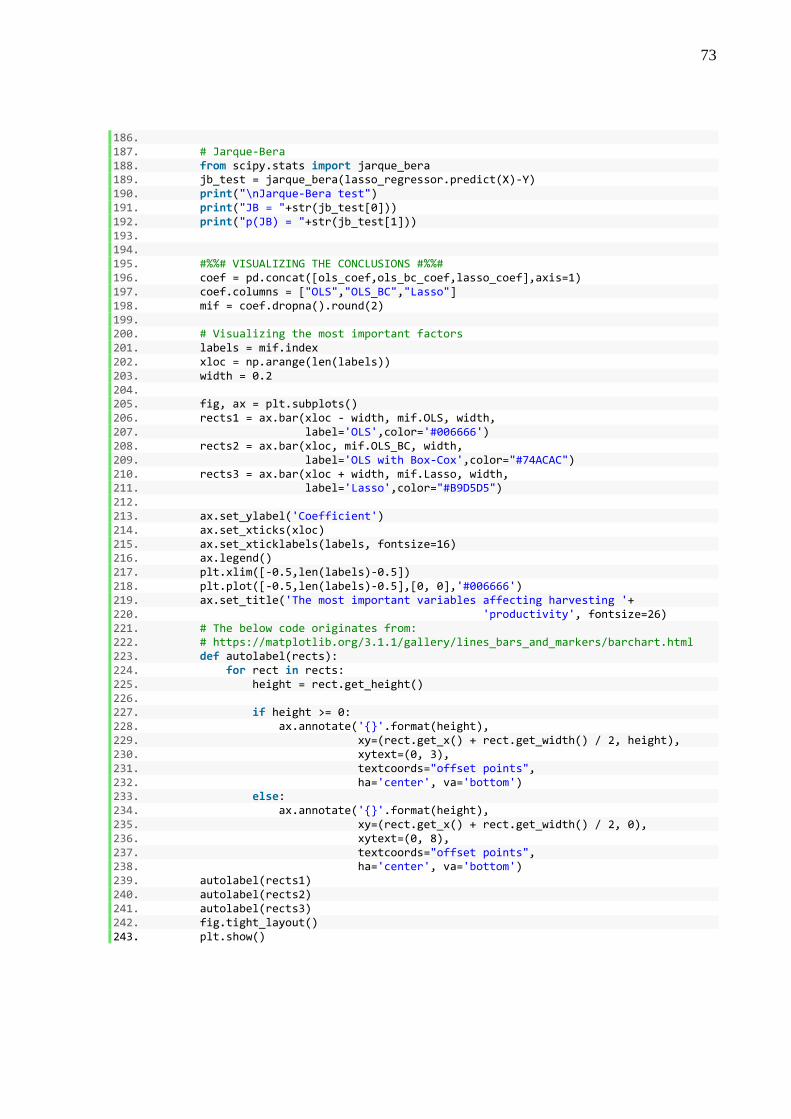
73
186. 187. # Jarque-Bera 188. from scipy.stats import jarque_bera 189. jb_test = jarque_bera(lasso_regressor.predict(X)-Y) 190. print("\nJarque-Bera test") 191. print("JB = "+str(jb_test[0])) 192. print("p(JB) = "+str(jb_test[1])) 193. 194. 195. #%%# VISUALIZING THE CONCLUSIONS #%%# 196. coef = pd.concat([ols_coef,ols_bc_coef,lasso_coef],axis=1) 197. coef.columns = ["OLS","OLS_BC","Lasso"] 198. mif = coef.dropna().round(2) 199. 200. # Visualizing the most important factors 201. labels = mif.index 202. xloc = np.arange(len(labels)) 203. width = 0.2 204. 205. fig, ax = plt.subplots() 206. rects1 = ax.bar(xloc - width, mif.OLS, width, 207. label='OLS',color='#006666') 208. rects2 = ax.bar(xloc, mif.OLS_BC, width, 209. label='OLS with Box-Cox',color="#74ACAC") 210. rects3 = ax.bar(xloc + width, mif.Lasso, width, 211. label='Lasso',color="#B9D5D5") 212. 213. ax.set_ylabel('Coefficient') 214. ax.set_xticks(xloc) 215. ax.set_xticklabels(labels, fontsize=16) 216. ax.legend() 217. plt.xlim([-0.5,len(labels)-0.5]) 218. plt.plot([-0.5,len(labels)-0.5],[0, 0],'#006666') 219. ax.set_title('The most important variables affecting harvesting '+ 220. 'productivity', fontsize=26) 221. # The below code originates from: 222. # https://matplotlib.org/3.1.1/gallery/lines_bars_and_markers/barchart.html 223. def autolabel(rects): 224. for rect in rects: 225. height = rect.get_height() 226. 227. if height >= 0: 228. ax.annotate('{}'.format(height), 229. xy=(rect.get_x() + rect.get_width() / 2, height), 230. xytext=(0, 3), 231. textcoords="offset points", 232. ha='center', va='bottom') 233. else: 234. ax.annotate('{}'.format(height), 235. xy=(rect.get_x() + rect.get_width() / 2, 0), 236. xytext=(0, 8), 237. textcoords="offset points", 238. ha='center', va='bottom') 239. autolabel(rects1) 240. autolabel(rects2) 241. autolabel(rects3) 242. fig.tight_layout() 243. plt.show()

74
A3 Python code: Data preprocessing and feature extraction
1. import os 2. import pandas as pd 3. import numpy as np 4. 5. def preprocess_data(folder_path): 6. 7. df = pd.DataFrame() 8. # Iterating through the log files in the folder 9. os.chdir(folder_path) 10. for filename in os.listdir(os.getcwd()): 11. 12. # The log data files in the folder are read one by one 13. data = pd.read_csv(filename, sep=';') 14. # Selecting necessary columns & omitting the first and last row 15. data = data.iloc[1:-1,np.r_[0:14,17:19,21,28,42:44,47,49:59]] 16. # The column names are simplified 17. data.rename(columns=lambda x: x.split()[::-1][0], inplace=True) 18. # Making sure that the number of felling cuts starts from zero 19. if int(data.NumberOfFellingCuts.min()) != 0: 20. data.loc[:,"NumberOfFellingCuts"] = (data.loc[:, 21. "NumberOfFellingCuts"]-int(data.NumberOfFellingCuts.min())) 22. # Calculating the number of felled trees in the data file 23. n_trees = int(data.NumberOfFellingCuts.max()) 24. # The data from the beginning (no trees felled yet) and the end 25. # (no trees to be cut anymore) of time-series are removed 26. data = data.loc[(data.NumberOfFellingCuts != 0) & 27. (data.NumberOfFellingCuts != n_trees),:] 28. 29. ## Identifying the work stages: 30. # Felling (F) and Processing (P) 31. for i in range(1,n_trees): 32. # Start by finding a subset of time-series data associated 33. # with number of felling cuts 34. subset = data[data.NumberOfFellingCuts == i].copy() 35. # Processing (felling and delimbing) the stem starts from the 36. # beginning of the subset. Now the harvester head is holding 37. # the stem, which is indicated by the thickness sensor value 38. # < 1000. Stage ends when the sensor, for the first time 39. # concerning the current subset, returns to 1000 indicating 40. # that the tree has been dropped and the felling head is not 41. # processing it any more. 42. procStart = subset.index[0] 43. procEnd = subset[subset.Paksuusanturi == 1000].index[0]-1 44. data.loc[procStart : procEnd, "WorkStage"] = "P" 45. # When for the last time, concerning the selected subset, the 46. # thickness sensor value drops below 1000, it means that the 47. # harvester has now sticked to a new tree that will be cutted 48. # soon. The tree "is being cut" until the end of the current 49. # subset, as being in the next subset indicates that number 50. # of felling cuts has increased by one and the tree has 51. # already been cut (delimbing and cross-cutting continues 52. # from that point). 53. felStart = subset.Paksuusanturi[::-1][subset.Paksuusanturi 54. == 1000].index[0]+1 55. felEnd = subset.index[-1] 56. data.loc[felStart : felEnd, "WorkStage"] = "F" 57. 58. # Moving (M) 59. # If driving speed is not zero, the harvester is moving

75
60. data.loc[data.Ajonopeus != 0 & data.WorkStage.isna(), 61. "WorkStage"] = "M" 62. 63. # Delays (D) 64. # When the RPM value of the engine < 1000, no work is being done 65. data.loc[(data.DieselRPM < 1000) & data.WorkStage.isna(), 66. "WorkStage"] = "D" 67. 68. # Other (O) 69. # Data points that do not fit into any of the other categories, 70. # are assigned to this stage. Other activities means e.g. crane 71. # movements and arranging and moving logs, branches and tops. 72. data.loc[data.WorkStage.isna(),"WorkStage"] = "O" 73. 74. # Creating work cycle indicator. The indicator differs from the 75. # NumberOfFellingCuts in a way that it starts already from the 76. # point when the harvester head has dropped the previous tree, 77. # whereas NOFC grows only after a new tree has been cut. 78. n_trees = int(data.NumberOfFellingCuts.max()) 79. for i in range(1,n_trees+1): 80. subset = data[data.NumberOfFellingCuts == i].copy() 81. next_cycle_start = subset[subset.WorkStage != "P"].index[0] 82. data.loc[subset.index[0]:next_cycle_start-1,"CycleNumber"]=i 83. data.loc[next_cycle_start:subset.index[-1],"CycleNumber"]=i+1 84. data = data.loc[(data.CycleNumber != 1) & 85. (data.CycleNumber != n_trees+1),:] 86. 87. # The delay times (e.g. breaks of the operator) are omitted 88. data = data[data["WorkStage"] != "D"] 89. 90. # Function calculates the distance between current and next tree 91. def calculate_intertree_distance(cycle): 92. lat1 = cycle.Latitude.iloc[0] 93. lng1 = cycle.Longitude.iloc[0] 94. lat2 = cycle.Latitude.iloc[-1] 95. lng2 = cycle.Longitude.iloc[-1] 96. lat1,lng1,lat2,lng2 = map(np.radians, [lat1,lng1,lat2,lng2]) 97. # Distance using Haversine formula 98. # Source: https://en.wikipedia.org/wiki/Haversine_formula 99. return 2*6373*np.arcsin(np.sqrt(np.sin((lat2-lat1)/2)** 100. 2+np.cos(lat1)*np.cos(lat2)*np.sin((lng2-lng1)/2)**2)) 101. 102. ## BUILDING THE FEATURES 103. # 1. Diameter of the first log collected from the tree 104. tree_diameter = [] 105. # 2. Share-% of time spend in felling during the cycle 106. tshare_F = [] 107. # 3. Share-% of time spend in processing (i.e. delimbing and 108. # cross-cutting) during the cycle 109. tshare_P = [] 110. # 4. Share-% of time spend in other activities during the cycle 111. tshare_O = [] 112. # 5. Average RPM during the work cycle 113. avg_rpm = [] 114. # 6. Average fuel consumption momentary during the work cycle 115. avg_fcm = [] 116. # 7-9. Dummy indicator variables for the tree species 117. species0 = [] 118. species1 = [] 119. species2 = [] 120. # 10. Distance between the last and the current tree 121. intertree_distance = [] 122. # 11. Altitude change between current and next tree

76
123. altitude_change = [] 124. # 12. The number of frame joint turns during the work cycle 125. num_FJ_turns = [] 126. # 13. Maximum driving speed between the trees 127. max_drive_speed = [] 128. # 14. Variable quantifying the crane movement complexity 129. crane_move_cplx1 = [] 130. # 15. Alternative variable for crane movement complexity 131. crane_move_cplx2 = [] 132. # 16. Non-delay time since starting the current fellings 133. time_since_start = [] 134. # TARGET: Produced volume of wood per time unit 135. productivity = [] 136. 137. # Iterating through work cycles (individual felled trees) 138. n_cycles = int(data.CycleNumber.max()) 139. for i in range(2,n_cycles+1): 140. # Find subset associated with processing of the current tree 141. cycle = data[data.CycleNumber == i] 142. # Logs-subset is the same as cycle-subset, but the records 143. # with log volume value corresponding to previous cycle have 144. # been removed 145. logs = cycle[cycle.NumberOfLogs != cycle.NumberOfLogs.min()] 146. numOfLogs=logs.NumberOfLogs.max()-(logs.NumberOfLogs.min()-1) 147. # Checking whether at least one log was collected from the 148. # current tree 149. if numOfLogs == numOfLogs: 150. # If yes, the following feature values are calculated from it 151. tree_diameter.append( 152. logs.AverageDiameter.unique().max()) 153. tshare_F.append( 154. cycle[cycle.WorkStage=="F"].WorkStage.count() 155. /cycle.WorkStage.count()) 156. tshare_P.append( 157. cycle[cycle.WorkStage=="P"].WorkStage.count() 158. /cycle.WorkStage.count()) 159. tshare_O.append( 160. cycle[cycle.WorkStage=="O"].WorkStage.count() 161. /cycle.WorkStage.count()) 162. avg_rpm.append(cycle.DieselRPM.mean()) 163. avg_fcm.append(cycle.FuelConsumptionMomentary.mean()) 164. species0.append( 165. int(logs.TreeSpecie.iloc[0] == 0)) 166. species1.append( 167. int(logs.TreeSpecie.iloc[0] == 1)) 168. species2.append( 169. int(logs.TreeSpecie.iloc[0] == 2)) 170. intertree_distance.append( 171. calculate_intertree_distance(cycle)) 172. altitude_change.append( 173. cycle.Altitude.iloc[-1]-cycle.Altitude.iloc[0]) 174. num_FJ_turns.append(((cycle["OhjausRunkoOhjaus-"] != 0). 175. astype(int).diff().abs().sum() + (cycle 176. ["OhjausRunkoOhjaus+"] != 0).astype(int).diff(). 177. abs().sum())) 178. max_drive_speed.append( 179. cycle.Ajonopeus.max()) 180. crane_move_cplx1.append( 181. (cycle.iloc[:,1:9].sum().sum())/(cycle.Time.count())) 182. crane_move_cplx2.append( 183. (cycle.iloc[:,1:9].diff(). 184. abs().sum().sum())/(cycle.Time.count())) 185. time_since_start.append(
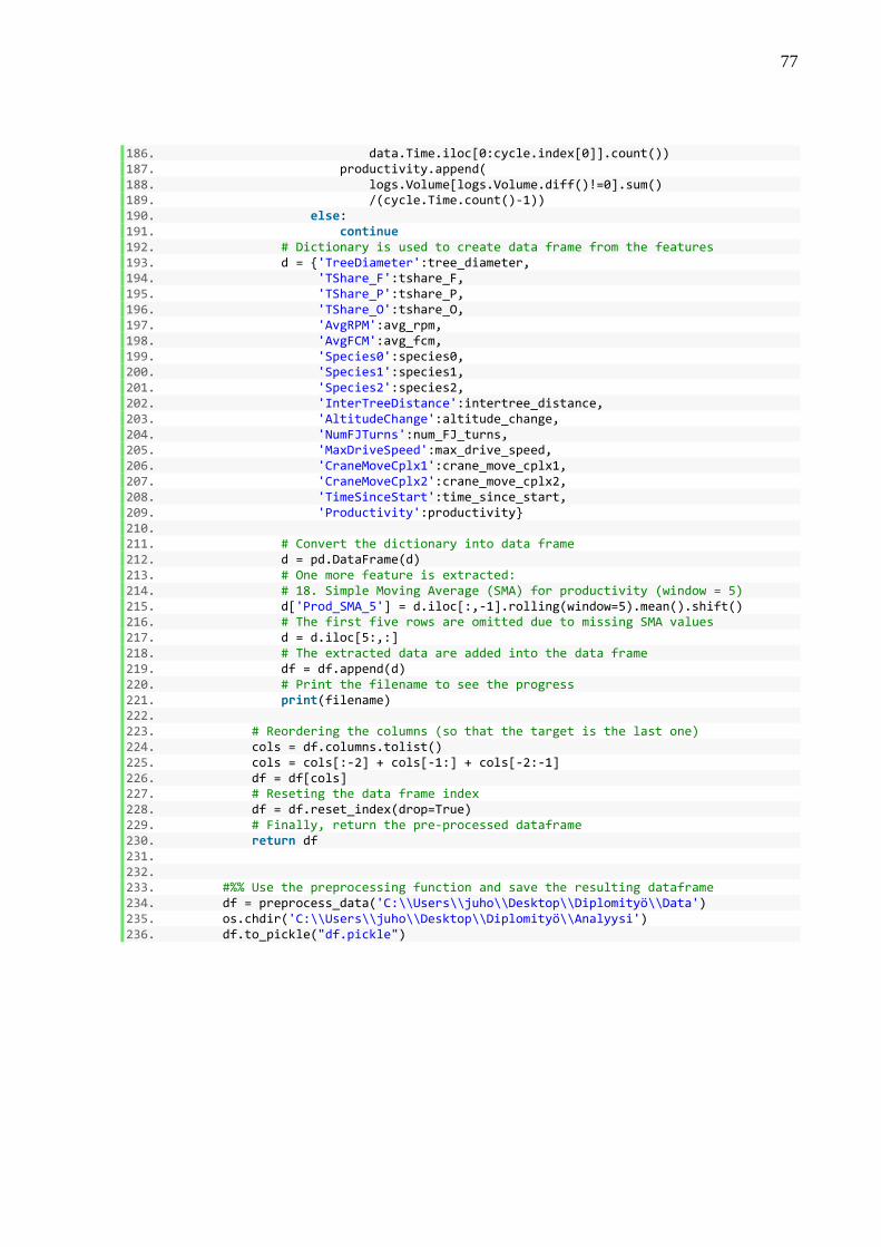
77
186. data.Time.iloc[0:cycle.index[0]].count()) 187. productivity.append( 188. logs.Volume[logs.Volume.diff()!=0].sum() 189. /(cycle.Time.count()-1)) 190. else: 191. continue 192. # Dictionary is used to create data frame from the features 193. d = {'TreeDiameter':tree_diameter, 194. 'TShare_F':tshare_F, 195. 'TShare_P':tshare_P, 196. 'TShare_O':tshare_O, 197. 'AvgRPM':avg_rpm, 198. 'AvgFCM':avg_fcm, 199. 'Species0':species0, 200. 'Species1':species1, 201. 'Species2':species2, 202. 'InterTreeDistance':intertree_distance, 203. 'AltitudeChange':altitude_change, 204. 'NumFJTurns':num_FJ_turns, 205. 'MaxDriveSpeed':max_drive_speed, 206. 'CraneMoveCplx1':crane_move_cplx1, 207. 'CraneMoveCplx2':crane_move_cplx2, 208. 'TimeSinceStart':time_since_start, 209. 'Productivity':productivity} 210. 211. # Convert the dictionary into data frame 212. d = pd.DataFrame(d) 213. # One more feature is extracted: 214. # 18. Simple Moving Average (SMA) for productivity (window = 5) 215. d['Prod_SMA_5'] = d.iloc[:,-1].rolling(window=5).mean().shift() 216. # The first five rows are omitted due to missing SMA values 217. d = d.iloc[5:,:] 218. # The extracted data are added into the data frame 219. df = df.append(d) 220. # Print the filename to see the progress 221. print(filename) 222. 223. # Reordering the columns (so that the target is the last one) 224. cols = df.columns.tolist() 225. cols = cols[:-2] + cols[-1:] + cols[-2:-1] 226. df = df[cols] 227. # Reseting the data frame index 228. df = df.reset_index(drop=True) 229. # Finally, return the pre-processed dataframe 230. return df 231. 232. 233. #%% Use the preprocessing function and save the resulting dataframe 234. df = preprocess_data('C:\\Users\\juho\\Desktop\\Diplomityö\\Data') 235. os.chdir('C:\\Users\\juho\\Desktop\\Diplomityö\\Analyysi') 236. df.to_pickle("df.pickle")


![Productivity in Mining[998]](https://static.fdocuments.net/doc/165x107/58859f151a28abd2498b6925/productivity-in-mining998.jpg)