Forest Carbon Accounting: Overview & Principles

CDM Capacity Development in Eastern and Southern Africa

1

Charlene Watson London School of Economics and Political Science

c.watson2@lse.ac.uk

Disclaimer The views expressed in this publication are those of the author and do not necessarily represent those of the United Nations, UNDP, UNEP, UNEP Risoe Centre or their Member States.

2

Forest Carbon Accounting: Overview & Principles Executive Summary Forests play an important role in the global carbon balance. As both carbon sources and sinks, they have the potential to form an important component in efforts to combat global climate change. Accounting for the carbon within forest ecosystems and changes in carbon stocks resulting from human activities is a necessary first step towards the better representation of forests in climate change policy at regional, national and global scales. The United Nations Development Programme (UNDP), as part of the UNDP-UNEP CDM Capacity Development Project for Eastern & Southern Africa, is seeking to promote carbon projects in sub-Saharan Africa, in the important bio-carbon sector and others. This report reinforces UNDP’s capacity building efforts by presenting the main principles, practices and challenges of carbon accounting in the forestry sector. Forest carbon accounting can be divided into three forms. Stock accounting assesses the magnitude of carbon stored in forest ecosystems at a single point in time. Emissions accounting assesses the net greenhouse gas emissions to the atmosphere resulting from forests. Emission reductions accounting assesses the decrease in emissions from project or policy activities, often so that they can be traded. Forest carbon accounting identifies the carbon-density of areas, providing information for low-carbon-impact land use planning. It prepares territories for accounting and reporting of emissions from the forestry sector. It allows comparison of the climate change impact of the forestry sector relative to other sectors, as well as allowing comparison between territories. Finally, it enables trade of project emission reductions on carbon markets and for emission reductions to be included in policy targets. Good practice in forest carbon accounting must be adhered to. In particular, transparency in methods and accuracy and precision in accounting are required for public and political acceptance of resultant estimates. A basic knowledge of the principles underlying forest carbon accounting is also beneficial. Understanding biomass dynamics and flows between carbon pools in forest ecosystems enables more effective accounting. The practice of forest carbon accounting requires clear identification of the accounting boundary in both space and time. Stratifying the forest into areas with similar carbon characteristics further improves the accuracy of carbon accounting. Data for accounting can be gathered from a variety of sources, including existing secondary data, remotely sensed data and primary data through field surveys. The amount of data from each source depends on the quality of the source as well as the trade-offs that must be made between accounting accuracy and costs of resources and time. All forest carbon accounting estimates contain uncertainty. Practitioners should identify, minimise where possible, and quantify this uncertainty through statistical analysis, published information and expert judgement. Uncertainty of model variables and components, once quantified, can be aggregated through simple propagation of errors or simulated through Monte Carlo analysis. The existence of substantial uncertainty can undermine efforts to reduce carbon emissions from forestry and can erode political support for the accounting process.

3

Forest carbon accounting guidance from the Intergovernmental Panel on Climate Change (IPCC) has become the primary source of information for methods, accounting equations and parameters. However, IPCC guidance is vast and often difficult to navigate. In response, a number of tools for forest carbon accounting have emerged. These vary in terms of geographical coverage, forestry activities and the carbon pools accounted for, as well as the level of data input required. In light of such diversity, practitioners require an understanding of the forest carbon accounting process, irrespective of whether these tools are utilised. Despite substantial progress in the field of forest carbon accounting over the last decade, challenges still remain. Terminology relating to forests and managed lands is ambiguous and requires standardisation between stakeholders. More scientific research into forest biomass characteristics is also required to better incorporate the heterogeneity of forests, their growth dynamics and the fate of carbon in harvested wood products into forest carbon accounting methods. Forest carbon accounting is a multi-disciplinary task. Building capacity is essential. Investment is also necessary to improve and standardise carbon accounting methods. If future climate change policy and strategy are to adequately reflect the substantial role forests play in the global carbon balance, good forest carbon accounting is imperative.

4

Table of Contents Executive Summary ...................................................................................................................................... 2 List of Figures ............................................................................................................................................... 5 1. Introduction ............................................................................................................................................. 6

1.1. Report structure ...........................................................................................................................................6 1.2. What is forest carbon accounting? ..............................................................................................................6

2. Principles of forest carbon accounting ....................................................................................................... 7 2.1. Accounting good practice .............................................................................................................................7 2.2. Biomass, carbon pools and stock accounting ..............................................................................................8 2.3. Approaches to emission accounting ......................................................................................................... 10 2.4. Accounting for emission reductions ......................................................................................................... 11

2.4.1. Baselines ............................................................................................................................................. 12 2.4.2. Additionality ........................................................................................................................................ 12 2.4.3. Leakage ............................................................................................................................................... 13 2.4.4. Permanence ........................................................................................................................................ 13

3. Practice of forest carbon accounting ....................................................................................................... 14 3.1. Establishing the accounting area .............................................................................................................. 14

3.2.1. Collating existing forest data .............................................................................................................. 16 3.2.2. Using remote sensing .......................................................................................................................... 16 3.2.3. Data from field sampling .................................................................................................................... 18

3.3. Accounting for forest carbon stocks ......................................................................................................... 18 3.3.1. Above-ground biomass (AGB) ............................................................................................................. 18 3.3.2. Below-ground biomass (BGB) ............................................................................................................. 19 3.3.3. Dead organic matter (wood)............................................................................................................... 20 3.3.4. Dead organic matter (litter) ................................................................................................................ 20 3.3.5. Soil organic matter (SOM) .................................................................................................................. 20

3.4. Accounting for forest carbon emissions ................................................................................................... 21 3.4.1. Accounting for carbon stock changes in carbon pools ........................................................................ 21 3.4.2. Accounting for carbon stored in harvested wood products (HWPs) ................................................... 21 3.4.3. Accounting for nitrous oxide and methane emissions from disturbances .......................................... 22

3.5. Quantifying uncertainty in carbon accounting ......................................................................................... 23 4. Guidance and tools for forest carbon accounting ..................................................................................... 24

4.1. IPCC guidelines .......................................................................................................................................... 24 4.2. Carbon accounting tools............................................................................................................................ 25 4.3. Bilan Carbone ............................................................................................................................................ 26

5. Challenges for forest carbon accounting .................................................................................................. 26 5.1. Clarifying terminology ............................................................................................................................... 26

5.1.1. Definition of ‘forest’ ............................................................................................................................ 26 5.1.2. Direct human-induced impacts ........................................................................................................... 27

5.2. Forest Characteristics ................................................................................................................................ 28 5.2.1. Heterogeneity of forests ..................................................................................................................... 28 5.2.2. Forest growth and equilibrium ........................................................................................................... 29 5.2.3. Accounting for harvested wood products ........................................................................................... 29

6. Conclusion ............................................................................................................................................. 30 7. Appendices ............................................................................................................................................ 31

7.1. Appendix I: References ............................................................................................................................. 31 7.2. Appendix II: Acronyms .............................................................................................................................. 36 7.3. Appendix III: Glossary ................................................................................................................................ 37 7.4. Appendix IV: Examples of default equations and data for forest carbon accounting ............................ 39

5

List of Tables

Table 1. Good practice for forest carbon accounting ...............................................................................................8 Table 2. Default forest biomass and annual biomass increment under tier 1 IPCC guidance .............................. 17 Table 3. Factors affecting forest carbon stocks ..................................................................................................... 28 Table A4:1. Exemplary above-ground biomass regression equations for tropical trees ...................................... 39 Table A4:2. Default mineral soil organic carbon stocks ........................................................................................ 39

List of Figures Figure 1. Diagrammatic Representation of Carbon Pools ....................................................................................... 9 Figure 2. Generalised flow of carbon between pools ........................................................................................... 10 Figure 3. Outline of the practice of forest carbon accounting .............................................................................. 15

6

1. Introduction

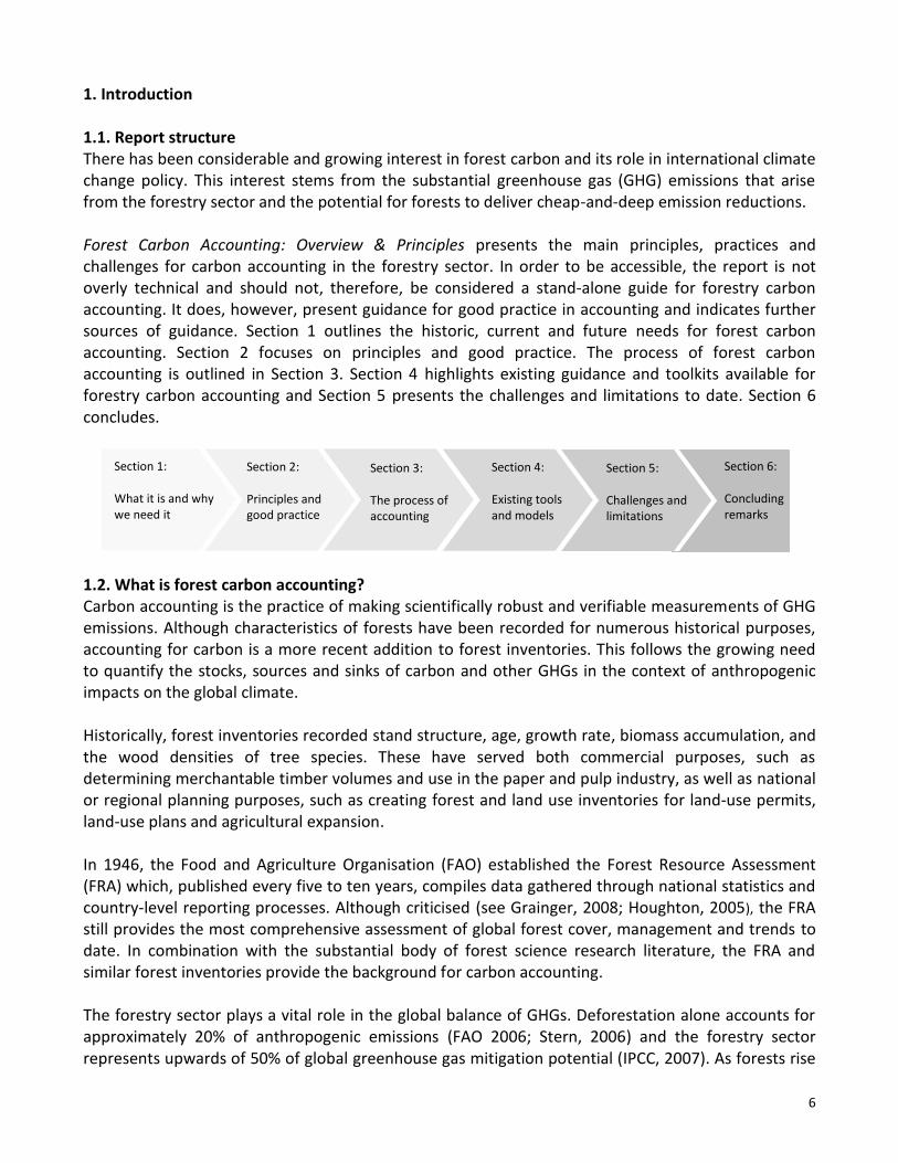
1.1. Report structure There has been considerable and growing interest in forest carbon and its role in international climate change policy. This interest stems from the substantial greenhouse gas (GHG) emissions that arise from the forestry sector and the potential for forests to deliver cheap-and-deep emission reductions. Forest Carbon Accounting: Overview & Principles presents the main principles, practices and challenges for carbon accounting in the forestry sector. In order to be accessible, the report is not overly technical and should not, therefore, be considered a stand-alone guide for forestry carbon accounting. It does, however, present guidance for good practice in accounting and indicates further sources of guidance. Section 1 outlines the historic, current and future needs for forest carbon accounting. Section 2 focuses on principles and good practice. The process of forest carbon accounting is outlined in Section 3. Section 4 highlights existing guidance and toolkits available for forestry carbon accounting and Section 5 presents the challenges and limitations to date. Section 6 concludes.

1.2. What is forest carbon accounting? Carbon accounting is the practice of making scientifically robust and verifiable measurements of GHG emissions. Although characteristics of forests have been recorded for numerous historical purposes, accounting for carbon is a more recent addition to forest inventories. This follows the growing need to quantify the stocks, sources and sinks of carbon and other GHGs in the context of anthropogenic impacts on the global climate. Historically, forest inventories recorded stand structure, age, growth rate, biomass accumulation, and the wood densities of tree species. These have served both commercial purposes, such as determining merchantable timber volumes and use in the paper and pulp industry, as well as national or regional planning purposes, such as creating forest and land use inventories for land-use permits, land-use plans and agricultural expansion. In 1946, the Food and Agriculture Organisation (FAO) established the Forest Resource Assessment (FRA) which, published every five to ten years, compiles data gathered through national statistics and country-level reporting processes. Although criticised (see Grainger, 2008; Houghton, 2005), the FRA still provides the most comprehensive assessment of global forest cover, management and trends to date. In combination with the substantial body of forest science research literature, the FRA and similar forest inventories provide the background for carbon accounting. The forestry sector plays a vital role in the global balance of GHGs. Deforestation alone accounts for approximately 20% of anthropogenic emissions (FAO 2006; Stern, 2006) and the forestry sector represents upwards of 50% of global greenhouse gas mitigation potential (IPCC, 2007). As forests rise

Section 1: What it is and why we need it

Section 2: Principles and good practice

Section 3: The process of accounting

Section 4: Existing tools and models

Section 5: Challenges and limitations

Section 6: Concluding remarks

7

up the climate change agenda, three types of forest carbon accounting have developed: stock accounting, emissions accounting and project emission reductions accounting.

Stock accounting Forest carbon stock accounting often forms a starting point for emissions and project-level accounting. Establishing the terrestrial carbon stock of a territory and average carbon stocks for particular land uses, stock accounting allows carbon-dense areas to be prioritised in regional land use planning. An early form of forest carbon accounting, emissions and emission reductions accounting have evolved from the principles established for stock accounting.

Emissions accounting Emissions accounting is necessary to assess the scale of emissions from the forestry sector relative to other sectors. It also aids realistic goal-setting for GHG emissions targets. Under the United Nations Framework Convention on Climate Change (UNFCCC) and the Kyoto Protocol, countries are mandated to undertake some land use, land use change and forestry (LULUCF) carbon accounting (see Box 1). With a significant portion of developing country emissions arising from the LULUCF sector, the forestry sector is likely to play a prominent role in climate change strategies in these countries.

Project emission reductions accounting Carbon accounting for forestry project emission reductions is required for both projects undertaken under the flexible mechanisms of the Kyoto Protocol and the voluntary carbon markets. Both necessitate good carbon accounting to ensure that emissions reductions are real, permanent and verifiable. For projects to generate tradable emission reductions, accounting methods between countries, regions and projects must be standardised in both developed and developing countries.

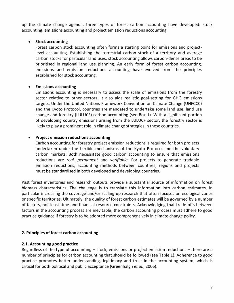
Past forest inventories and research outputs provide a substantial source of information on forest biomass characteristics. The challenge is to translate this information into carbon estimates, in particular increasing the coverage and/or scaling-up research that often focuses on ecological zones or specific territories. Ultimately, the quality of forest carbon estimates will be governed by a number of factors, not least time and financial resource constraints. Acknowledging that trade-offs between factors in the accounting process are inevitable, the carbon accounting process must adhere to good practice guidance if forestry is to be adopted more comprehensively in climate change policy. 2. Principles of forest carbon accounting 2.1. Accounting good practice Regardless of the type of accounting – stock, emissions or project emission reductions – there are a number of principles for carbon accounting that should be followed (see Table 1). Adherence to good practice promotes better understanding, legitimacy and trust in the accounting system, which is critical for both political and public acceptance (Greenhalgh et al., 2006).

8

Although publications commonly discuss ‘carbon’ accounting, completeness calls for the inclusion of other relevant GHGs in emissions and project emission reductions accounting. Thus, carbon accounting often refers to accounting of carbon dioxide equivalent (CO2e), a metric which allows standardisation of the six major GHGs based on their global warming potential. In the forestry sector, management regimes influence the scale of methane (CH4) and nitrous oxide (N2O) emissions in addition to carbon emissions. Methane emissions result from burning and decomposition of organic matter in oxygen-free environments, such as waterlogged soils. Nitrous oxide is emitted during burning, decomposition of organic matter, soil organic matter mineralisation and land fertilisation by nitrogen fertilisers. Although these gases tend to be produced in lower volumes than CO2 they have greater global warming potential. To adhere to good practice, CH4 and N2O emissions should be fully accounted for where significant. However, where minor, meaning less than 1% of the total (IPCC, 2003), such emissions can be omitted from accounting.

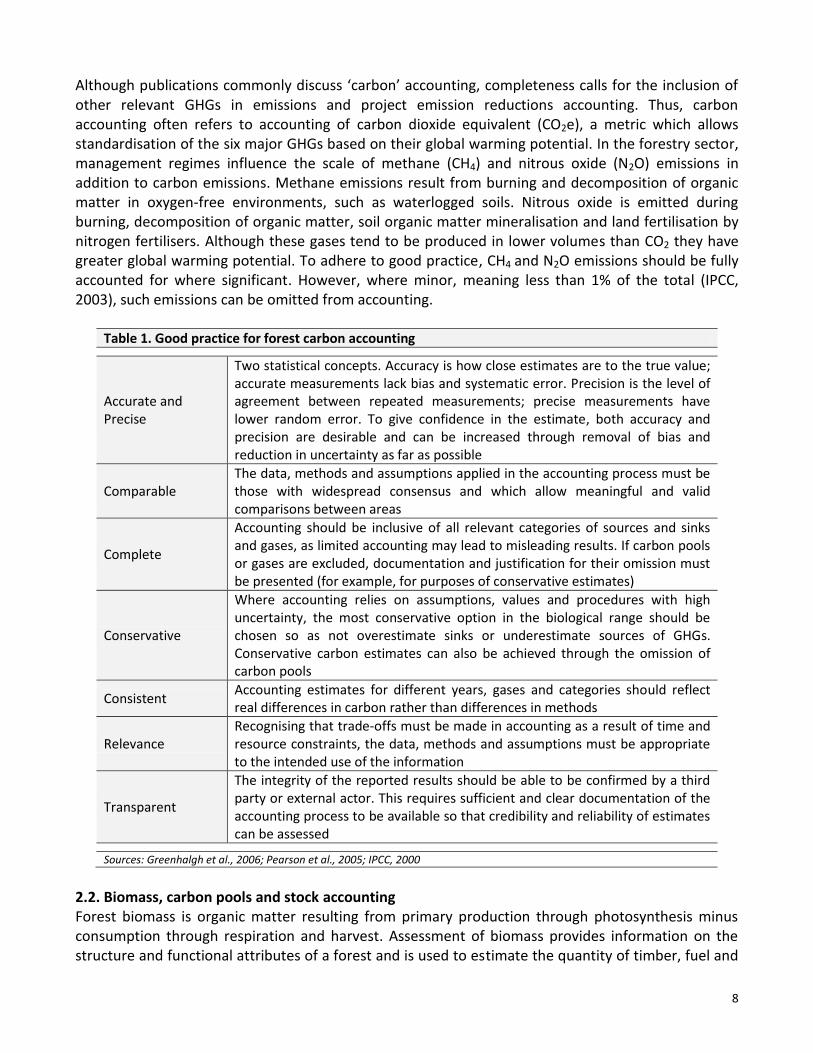
Table 1. Good practice for forest carbon accounting

Accurate and Precise

Two statistical concepts. Accuracy is how close estimates are to the true value; accurate measurements lack bias and systematic error. Precision is the level of agreement between repeated measurements; precise measurements have lower random error. To give confidence in the estimate, both accuracy and precision are desirable and can be increased through removal of bias and reduction in uncertainty as far as possible

Comparable The data, methods and assumptions applied in the accounting process must be those with widespread consensus and which allow meaningful and valid comparisons between areas

Complete

Accounting should be inclusive of all relevant categories of sources and sinks and gases, as limited accounting may lead to misleading results. If carbon pools or gases are excluded, documentation and justification for their omission must be presented (for example, for purposes of conservative estimates)

Conservative

Where accounting relies on assumptions, values and procedures with high uncertainty, the most conservative option in the biological range should be chosen so as not overestimate sinks or underestimate sources of GHGs. Conservative carbon estimates can also be achieved through the omission of carbon pools

Consistent Accounting estimates for different years, gases and categories should reflect real differences in carbon rather than differences in methods

Relevance Recognising that trade-offs must be made in accounting as a result of time and resource constraints, the data, methods and assumptions must be appropriate to the intended use of the information

Transparent

The integrity of the reported results should be able to be confirmed by a third party or external actor. This requires sufficient and clear documentation of the accounting process to be available so that credibility and reliability of estimates can be assessed

Sources: Greenhalgh et al., 2006; Pearson et al., 2005; IPCC, 2000

2.2. Biomass, carbon pools and stock accounting Forest biomass is organic matter resulting from primary production through photosynthesis minus consumption through respiration and harvest. Assessment of biomass provides information on the structure and functional attributes of a forest and is used to estimate the quantity of timber, fuel and

9

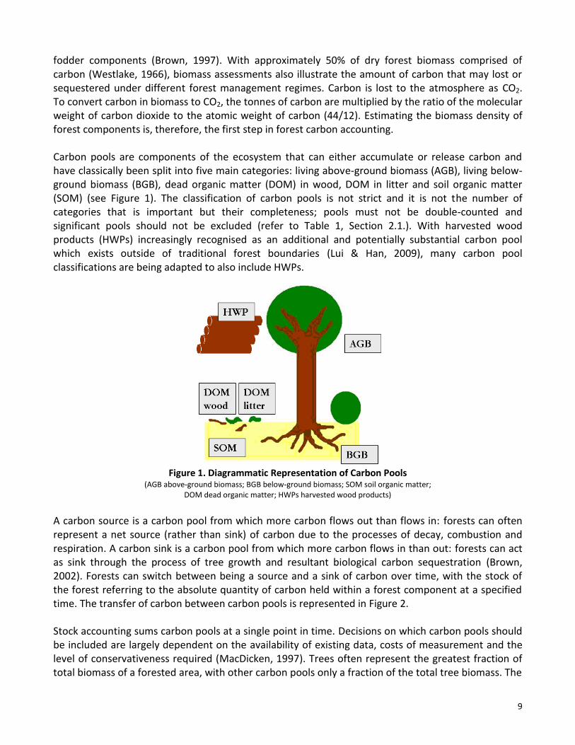
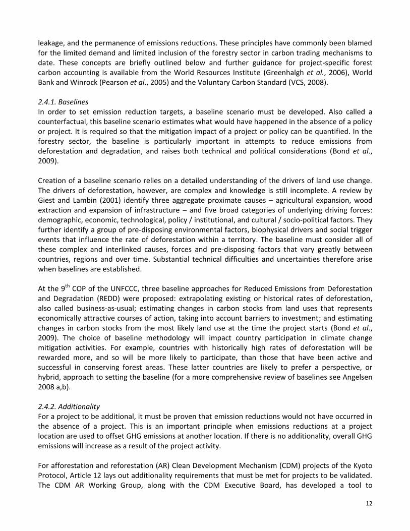
fodder components (Brown, 1997). With approximately 50% of dry forest biomass comprised of carbon (Westlake, 1966), biomass assessments also illustrate the amount of carbon that may lost or sequestered under different forest management regimes. Carbon is lost to the atmosphere as CO2. To convert carbon in biomass to CO2, the tonnes of carbon are multiplied by the ratio of the molecular weight of carbon dioxide to the atomic weight of carbon (44/12). Estimating the biomass density of forest components is, therefore, the first step in forest carbon accounting. Carbon pools are components of the ecosystem that can either accumulate or release carbon and have classically been split into five main categories: living above-ground biomass (AGB), living below-ground biomass (BGB), dead organic matter (DOM) in wood, DOM in litter and soil organic matter (SOM) (see Figure 1). The classification of carbon pools is not strict and it is not the number of categories that is important but their completeness; pools must not be double-counted and significant pools should not be excluded (refer to Table 1, Section 2.1.). With harvested wood products (HWPs) increasingly recognised as an additional and potentially substantial carbon pool which exists outside of traditional forest boundaries (Lui & Han, 2009), many carbon pool classifications are being adapted to also include HWPs.

Figure 1. Diagrammatic Representation of Carbon Pools

(AGB above-ground biomass; BGB below-ground biomass; SOM soil organic matter; DOM dead organic matter; HWPs harvested wood products)

A carbon source is a carbon pool from which more carbon flows out than flows in: forests can often represent a net source (rather than sink) of carbon due to the processes of decay, combustion and respiration. A carbon sink is a carbon pool from which more carbon flows in than out: forests can act as sink through the process of tree growth and resultant biological carbon sequestration (Brown, 2002). Forests can switch between being a source and a sink of carbon over time, with the stock of the forest referring to the absolute quantity of carbon held within a forest component at a specified time. The transfer of carbon between carbon pools is represented in Figure 2. Stock accounting sums carbon pools at a single point in time. Decisions on which carbon pools should be included are largely dependent on the availability of existing data, costs of measurement and the level of conservativeness required (MacDicken, 1997). Trees often represent the greatest fraction of total biomass of a forested area, with other carbon pools only a fraction of the total tree biomass. The

10

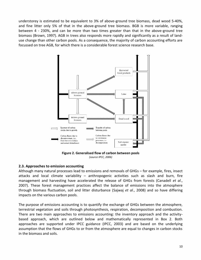
understorey is estimated to be equivalent to 3% of above-ground tree biomass, dead wood 5-40%, and fine litter only 5% of that in the above-ground tree biomass. BGB is more variable, ranging between 4 - 230%, and can be more than two times greater than that in the above-ground tree biomass (Brown, 1997). AGB in trees also responds more rapidly and significantly as a result of land-use change than other carbon pools. As a consequence, the majority of carbon accounting efforts are focussed on tree AGB, for which there is a considerable forest science research base.

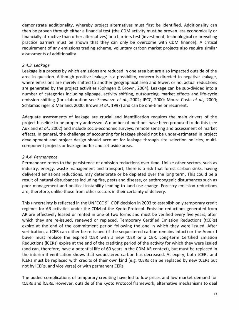
Figure 2. Generalised flow of carbon between pools

(source IPCC, 2006)

2.3. Approaches to emission accounting Although many natural processes lead to emissions and removals of GHGs – for example, fires, insect attacks and local climate variability – anthropogenic activities such as slash and burn, fire management and harvesting have accelerated the release of GHGs from forests (Canadell et al., 2007). These forest management practices affect the balance of emissions into the atmosphere through biomass fluctuation, soil and litter disturbance (Sajwaj et al., 2008) and so have differing impacts on the various carbon pools. The purpose of emissions accounting is to quantify the exchange of GHGs between the atmosphere, terrestrial vegetation and soils through photosynthesis, respiration, decomposition and combustion. There are two main approaches to emissions accounting: the inventory approach and the activity-based approach, which are outlined below and mathematically represented in Box 2. Both approaches are supported under IPCC guidance (IPCC, 2003) and are based on the underlying assumption that the flows of GHGs to or from the atmosphere are equal to changes in carbon stocks in the biomass and soils.

11

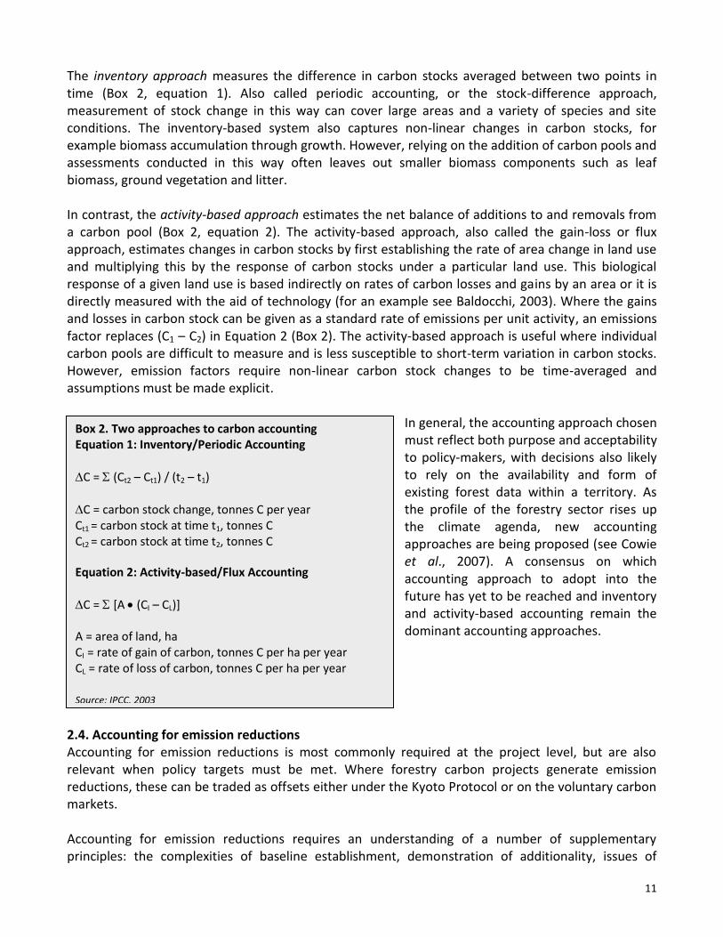
The inventory approach measures the difference in carbon stocks averaged between two points in time (Box 2, equation 1). Also called periodic accounting, or the stock-difference approach, measurement of stock change in this way can cover large areas and a variety of species and site conditions. The inventory-based system also captures non-linear changes in carbon stocks, for example biomass accumulation through growth. However, relying on the addition of carbon pools and assessments conducted in this way often leaves out smaller biomass components such as leaf biomass, ground vegetation and litter. In contrast, the activity-based approach estimates the net balance of additions to and removals from a carbon pool (Box 2, equation 2). The activity-based approach, also called the gain-loss or flux approach, estimates changes in carbon stocks by first establishing the rate of area change in land use and multiplying this by the response of carbon stocks under a particular land use. This biological response of a given land use is based indirectly on rates of carbon losses and gains by an area or it is directly measured with the aid of technology (for an example see Baldocchi, 2003). Where the gains and losses in carbon stock can be given as a standard rate of emissions per unit activity, an emissions factor replaces (C1 – C2) in Equation 2 (Box 2). The activity-based approach is useful where individual carbon pools are difficult to measure and is less susceptible to short-term variation in carbon stocks. However, emission factors require non-linear carbon stock changes to be time-averaged and assumptions must be made explicit.

In general, the accounting approach chosen must reflect both purpose and acceptability to policy-makers, with decisions also likely to rely on the availability and form of existing forest data within a territory. As the profile of the forestry sector rises up the climate agenda, new accounting approaches are being proposed (see Cowie et al., 2007). A consensus on which accounting approach to adopt into the future has yet to be reached and inventory and activity-based accounting remain the dominant accounting approaches.

2.4. Accounting for emission reductions Accounting for emission reductions is most commonly required at the project level, but are also relevant when policy targets must be met. Where forestry carbon projects generate emission reductions, these can be traded as offsets either under the Kyoto Protocol or on the voluntary carbon markets. Accounting for emission reductions requires an understanding of a number of supplementary principles: the complexities of baseline establishment, demonstration of additionality, issues of

Box 2. Two approaches to carbon accounting Equation 1: Inventory/Periodic Accounting

C = (Ct2 – Ct1) / (t2 – t1)

C = carbon stock change, tonnes C per year Ct1 = carbon stock at time t1, tonnes C Ct2 = carbon stock at time t2, tonnes C

Equation 2: Activity-based/Flux Accounting

C = [A (CI – CL)] A = area of land, ha CI = rate of gain of carbon, tonnes C per ha per year CL = rate of loss of carbon, tonnes C per ha per year

Source: IPCC, 2003

12

leakage, and the permanence of emissions reductions. These principles have commonly been blamed for the limited demand and limited inclusion of the forestry sector in carbon trading mechanisms to date. These concepts are briefly outlined below and further guidance for project-specific forest carbon accounting is available from the World Resources Institute (Greenhalgh et al., 2006), World Bank and Winrock (Pearson et al., 2005) and the Voluntary Carbon Standard (VCS, 2008). 2.4.1. Baselines In order to set emission reduction targets, a baseline scenario must be developed. Also called a counterfactual, this baseline scenario estimates what would have happened in the absence of a policy or project. It is required so that the mitigation impact of a project or policy can be quantified. In the forestry sector, the baseline is particularly important in attempts to reduce emissions from deforestation and degradation, and raises both technical and political considerations (Bond et al., 2009). Creation of a baseline scenario relies on a detailed understanding of the drivers of land use change. The drivers of deforestation, however, are complex and knowledge is still incomplete. A review by Giest and Lambin (2001) identify three aggregate proximate causes – agricultural expansion, wood extraction and expansion of infrastructure – and five broad categories of underlying driving forces: demographic, economic, technological, policy / institutional, and cultural / socio-political factors. They further identify a group of pre-disposing environmental factors, biophysical drivers and social trigger events that influence the rate of deforestation within a territory. The baseline must consider all of these complex and interlinked causes, forces and pre-disposing factors that vary greatly between countries, regions and over time. Substantial technical difficulties and uncertainties therefore arise when baselines are established. At the 9th COP of the UNFCCC, three baseline approaches for Reduced Emissions from Deforestation and Degradation (REDD) were proposed: extrapolating existing or historical rates of deforestation, also called business-as-usual; estimating changes in carbon stocks from land uses that represents economically attractive courses of action, taking into account barriers to investment; and estimating changes in carbon stocks from the most likely land use at the time the project starts (Bond et al., 2009). The choice of baseline methodology will impact country participation in climate change mitigation activities. For example, countries with historically high rates of deforestation will be rewarded more, and so will be more likely to participate, than those that have been active and successful in conserving forest areas. These latter countries are likely to prefer a perspective, or hybrid, approach to setting the baseline (for a more comprehensive review of baselines see Angelsen 2008 a,b). 2.4.2. Additionality For a project to be additional, it must be proven that emission reductions would not have occurred in the absence of a project. This is an important principle when emissions reductions at a project location are used to offset GHG emissions at another location. If there is no additionality, overall GHG emissions will increase as a result of the project activity. For afforestation and reforestation (AR) Clean Development Mechanism (CDM) projects of the Kyoto Protocol, Article 12 lays out additionality requirements that must be met for projects to be validated. The CDM AR Working Group, along with the CDM Executive Board, has developed a tool to

13

demonstrate additionality, whereby project alternatives must first be identified. Additionality can then be proven through either a financial test (the CDM activity must be proven less economically or financially attractive than other alternatives) or a barriers test (investment, technological or prevailing practice barriers must be shown that they can only be overcome with CDM finance). A critical requirement of any emissions trading scheme, voluntary carbon market projects also require similar assessments of additionality. 2.4.3. Leakage Leakage is a process by which emissions are reduced in one area but are also impacted outside of the area in question. Although positive leakage is a possibility, concern is directed to negative leakage, where emissions are merely shifted to another geographical area and fewer, or no, actual reductions are generated by the project activities (Sohngen & Brown, 2004). Leakage can be sub-divided into a number of categories including slippage, activity shifting, outsourcing, market effects and life-cycle emission shifting (for elaboration see Schwarze et al., 2002; IPCC, 2000; Moura-Costa et al., 2000; Schlamadinger & Marland, 2000; Brown et al., 1997) and can be one-time or recurrent. Adequate assessments of leakage are crucial and identification requires the main drivers of the project baseline to be properly addressed. A number of methods have been proposed to do this (see Aukland et al., 2002) and include socio-economic surveys, remote sensing and assessment of market effects. In general, the challenge of accounting for leakage should not be under-estimated in project development and project design should account for leakage through site selection policies, multi-component projects or leakage buffer and set-aside areas. 2.4.4. Permanence Permanence refers to the persistence of emission reductions over time. Unlike other sectors, such as industry, energy, waste management and transport, there is a risk that forest carbon sinks, having delivered emissions reductions, may deteriorate or be depleted over the long term. This could be a result of natural disturbances including fire, pests and disease, or anthropogenic disturbances such as poor management and political instability leading to land-use change. Forestry emission reductions are, therefore, unlike those from other sectors in their certainty of delivery. This uncertainty is reflected in the UNFCCC 9th COP decision in 2003 to establish only temporary credit regimes for AR activities under the CDM of the Kyoto Protocol. Emission reductions generated from AR are effectively leased or rented in one of two forms and must be verified every five years, after which they are re-issued, renewed or replaced. Temporary Certified Emission Reductions (tCERs) expire at the end of the commitment period following the one in which they were issued. After verification, a tCER can either be re-issued (if the sequestered carbon remains intact) or the Annex I buyer must replace the expired tCER with a new tCER or a CER. Long-term Certified Emission Reductions (lCERs) expire at the end of the crediting period of the activity for which they were issued (and can, therefore, have a potential life of 60 years in the CDM AR context), but must be replaced in the interim if verification shows that sequestered carbon has decreased. At expiry, both tCERs and lCERs must be replaced with credits of their own kind (e.g. tCERs can be replaced by new tCERs but not by lCERs, and vice versa) or with permanent CERs. The added complications of temporary crediting have led to low prices and low market demand for tCERs and lCERs. However, outside of the Kyoto Protocol framework, alternative mechanisms to deal

14

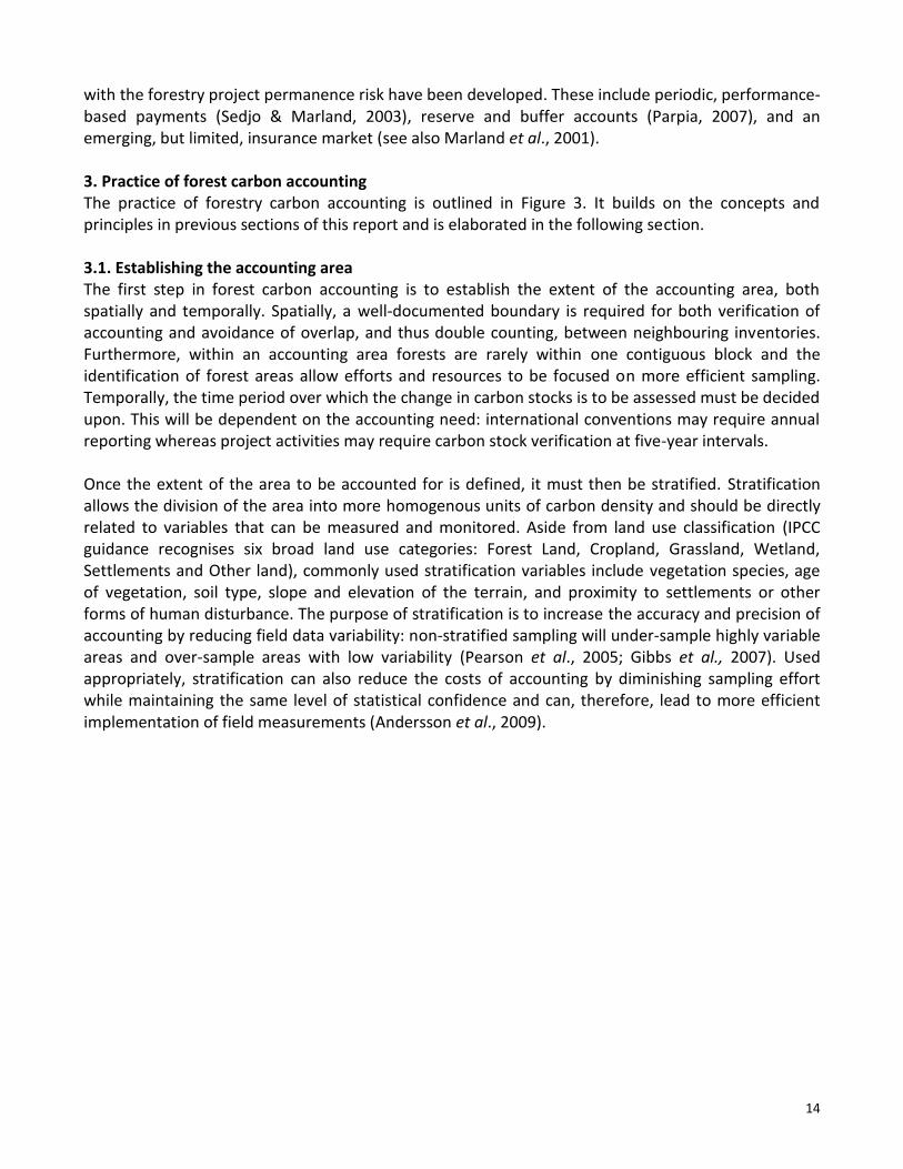
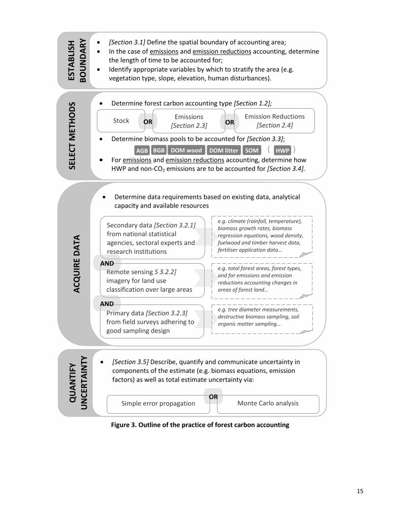
with the forestry project permanence risk have been developed. These include periodic, performance-based payments (Sedjo & Marland, 2003), reserve and buffer accounts (Parpia, 2007), and an emerging, but limited, insurance market (see also Marland et al., 2001). 3. Practice of forest carbon accounting The practice of forestry carbon accounting is outlined in Figure 3. It builds on the concepts and principles in previous sections of this report and is elaborated in the following section. 3.1. Establishing the accounting area The first step in forest carbon accounting is to establish the extent of the accounting area, both spatially and temporally. Spatially, a well-documented boundary is required for both verification of accounting and avoidance of overlap, and thus double counting, between neighbouring inventories. Furthermore, within an accounting area forests are rarely within one contiguous block and the identification of forest areas allow efforts and resources to be focused on more efficient sampling. Temporally, the time period over which the change in carbon stocks is to be assessed must be decided upon. This will be dependent on the accounting need: international conventions may require annual reporting whereas project activities may require carbon stock verification at five-year intervals. Once the extent of the area to be accounted for is defined, it must then be stratified. Stratification allows the division of the area into more homogenous units of carbon density and should be directly related to variables that can be measured and monitored. Aside from land use classification (IPCC guidance recognises six broad land use categories: Forest Land, Cropland, Grassland, Wetland, Settlements and Other land), commonly used stratification variables include vegetation species, age of vegetation, soil type, slope and elevation of the terrain, and proximity to settlements or other forms of human disturbance. The purpose of stratification is to increase the accuracy and precision of accounting by reducing field data variability: non-stratified sampling will under-sample highly variable areas and over-sample areas with low variability (Pearson et al., 2005; Gibbs et al., 2007). Used appropriately, stratification can also reduce the costs of accounting by diminishing sampling effort while maintaining the same level of statistical confidence and can, therefore, lead to more efficient implementation of field measurements (Andersson et al., 2009).

15

Figure 3. Outline of the practice of forest carbon accounting

QU

AN

TIFY

U

NC

ERTA

INTY

SELE

CT

MET

HO

DS

AC

QU

IRE

DA

TA

ESTA

BLI

SH

BO

UN

DA

RY

[Section 3.1] Define the spatial boundary of accounting area;

In the case of emissions and emission reductions accounting, determine the length of time to be accounted for;

Identify appropriate variables by which to stratify the area (e.g. vegetation type, slope, elevation, human disturbances).

Determine data requirements based on existing data, analytical capacity and available resources

Remote sensing S 3.2.2] imagery for land use classification over large areas

Secondary data [Section 3.2.1] from national statistical agencies, sectoral experts and research institutions

Primary data [Section 3.2.3] from field surveys adhering to good sampling design

Determine forest carbon accounting type [Section 1.2];

Determine biomass pools to be accounted for [Section 3.3];

( ) For emissions and emission reductions accounting, determine how

HWP and non-CO2 emissions are to be accounted for [Section 3.4].

Emission Reductions [Section 2.4]

Stock Emissions

[Section 2.3]

[Section 3.5] Describe, quantify and communicate uncertainty in components of the estimate (e.g. biomass equations, emission factors) as well as total estimate uncertainty via:

Monte Carlo analysis Simple error propagation

e.g. tree diameter measurements, destructive biomass sampling, soil organic matter sampling…

OR

AND

AND

OR OR

AGB DOM litter DOM wood SOM BGB HWP

e.g. climate (rainfall, temperature), biomass growth rates, biomass regression equations, wood density, fuelwood and timber harvest data, fertiliser application data…

e.g. total forest areas, forest types, and for emissions and emission reductions accounting changes in areas of forest land…

16

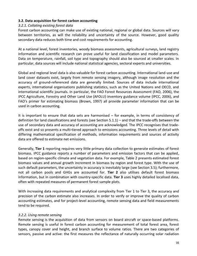
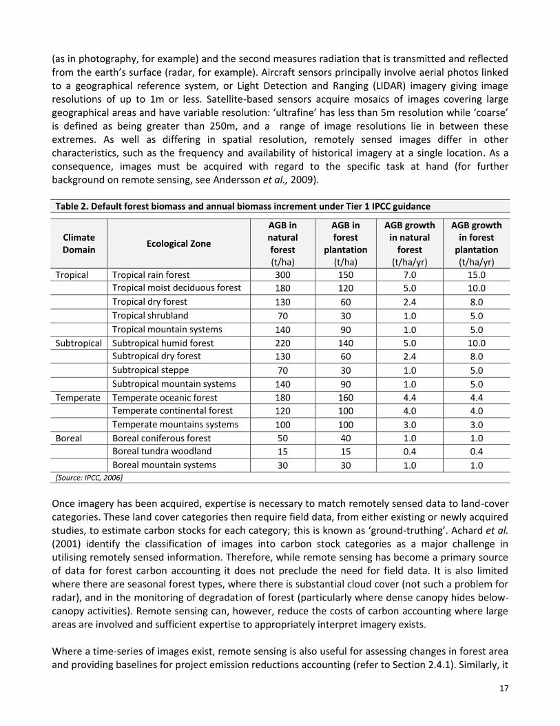
3.2. Data acquisition for forest carbon accounting 3.2.1. Collating existing forest data Forest carbon accounting can make use of existing national, regional or global data. Sources will vary between territories, as will the reliability and uncertainty of the source. However, good quality secondary data reduces both time and cost requirements for accounting. At a national level, forest inventories, woody biomass assessments, agricultural surveys, land registry information and scientific research can prove useful for land classification and model parameters. Data on temperature, rainfall, soil type and topography should also be sourced at smaller scales. In particular, data sources will include national statistical agencies, sectoral experts and universities. Global and regional level data is also valuable for forest carbon accounting. International land-use and land cover datasets exist, largely from remote sensing imagery, although image resolution and the accuracy of ground-referenced data are generally limited. Sources of data include international experts, international organisations publishing statistics, such as the United Nations and OECD, and international scientific journals. In particular, the FAO Forest Resources Assessment (FAO, 2006), the IPCC Agriculture, Forestry and Other Land Use (AFOLU) inventory guidance volume (IPCC, 2006), and FAO’s primer for estimating biomass (Brown, 1997) all provide parameter information that can be used in carbon accounting. It is important to ensure that data sets are harmonised – for example, in terms of consistency of definition for land classifications and forests (see Section 5.1.1) – and that the trade-offs between the use of secondary data and accuracy of accounting are acknowledged. The IPCC recognises that trade-offs exist and so presents a multi-tiered approach to emissions accounting. Three levels of detail with differing mathematical specification of methods, information requirements and sources of activity data are offered to estimate net emissions. Generally, Tier 1 reporting requires very little primary data collection to generate estimates of forest biomass. IPCC guidance reports a number of parameters and emission factors that can be applied, based on region-specific climate and vegetation data. For example, Table 2 presents estimated forest biomass values and annual growth increment in biomass by region and forest type. With the use of such default parameters, the uncertainty in accuracy is inevitably large (see Section 3.5); furthermore, not all carbon pools and GHGs are accounted for. Tier 2 also utilises default forest biomass information, but in combination with country-specific data. Tier 3 uses highly detailed localised data, often with repeated measures of permanent forest sample plots. With increasing data requirements and analytical complexity from Tier 1 to Tier 3, the accuracy and precision of the carbon estimate also increases. In order to verify or improve the quality of carbon accounting estimates, and for project-level accounting, remote sensing data and field measurements tend to be required. 3.2.2. Using remote sensing Remote sensing is the acquisition of data from sensors on board aircraft or space-based platforms. Remote sensing is useful in forest carbon accounting for measurement of total forest area, forest types, canopy cover and height, and branch surface to volume ratios. There are two categories of sensors, passive and active: the first measures the reflectance of naturally occurring solar radiation

17

(as in photography, for example) and the second measures radiation that is transmitted and reflected from the earth’s surface (radar, for example). Aircraft sensors principally involve aerial photos linked to a geographical reference system, or Light Detection and Ranging (LIDAR) imagery giving image resolutions of up to 1m or less. Satellite-based sensors acquire mosaics of images covering large geographical areas and have variable resolution: ‘ultrafine’ has less than 5m resolution while ‘coarse’ is defined as being greater than 250m, and a range of image resolutions lie in between these extremes. As well as differing in spatial resolution, remotely sensed images differ in other characteristics, such as the frequency and availability of historical imagery at a single location. As a consequence, images must be acquired with regard to the specific task at hand (for further background on remote sensing, see Andersson et al., 2009). Table 2. Default forest biomass and annual biomass increment under Tier 1 IPCC guidance

Climate Domain

Ecological Zone

AGB in natural forest (t/ha)

AGB in forest

plantation (t/ha)

AGB growth in natural

forest (t/ha/yr)

AGB growth in forest

plantation (t/ha/yr)

Tropical Tropical rain forest 300 150 7.0 15.0 Tropical moist deciduous forest 180 120 5.0 10.0

Tropical dry forest 130 60 2.4 8.0

Tropical shrubland 70 30 1.0 5.0

Tropical mountain systems 140 90 1.0 5.0 Subtropical Subtropical humid forest 220 140 5.0 10.0 Subtropical dry forest 130 60 2.4 8.0

Subtropical steppe 70 30 1.0 5.0

Subtropical mountain systems 140 90 1.0 5.0 Temperate Temperate oceanic forest 180 160 4.4 4.4 Temperate continental forest 120 100 4.0 4.0

Temperate mountains systems 100 100 3.0 3.0 Boreal Boreal coniferous forest 50 40 1.0 1.0 Boreal tundra woodland 15 15 0.4 0.4

Boreal mountain systems 30 30 1.0 1.0 [Source: IPCC, 2006]

Once imagery has been acquired, expertise is necessary to match remotely sensed data to land-cover categories. These land cover categories then require field data, from either existing or newly acquired studies, to estimate carbon stocks for each category; this is known as ‘ground-truthing’. Achard et al. (2001) identify the classification of images into carbon stock categories as a major challenge in utilising remotely sensed information. Therefore, while remote sensing has become a primary source of data for forest carbon accounting it does not preclude the need for field data. It is also limited where there are seasonal forest types, where there is substantial cloud cover (not such a problem for radar), and in the monitoring of degradation of forest (particularly where dense canopy hides below-canopy activities). Remote sensing can, however, reduce the costs of carbon accounting where large areas are involved and sufficient expertise to appropriately interpret imagery exists. Where a time-series of images exist, remote sensing is also useful for assessing changes in forest area and providing baselines for project emission reductions accounting (refer to Section 2.4.1). Similarly, it

18

has been promoted for long-term monitoring, reporting and verification for emission reductions targets. Remote sensing is replicable, standardised globally, implemented at a national level and is stable over the long term (UN-REDD, 2008). Of course, the applicability of remote sensing is highly dependent on the monitoring requirements: illegal operations require frequent remote sensing, forest fires require ad hoc and intense remote sensing, and timing of national forest inventories will be set by country priorities. With technology for remote sensing and methods for analysis of the data improving rapidly, it is likely to play a substantial role in forest carbon accounting into the future. 3.2.3. Data from field sampling Actual field data is preferable to default data for forest carbon accounting and is required to verify remotely sensed information and generalised data sets. Gathering field measurements for forest carbon accounting requires sampling as complete enumerations are neither practical nor efficient. By definition, sampling infers information about an entire population by observing only a fraction of it. In order to confidently scale up this data to the required geographical level, proper sampling design is vital. A central concept in sampling design theory is the need to reduce bias, often calling for simple random sampling. For carbon inventory purposes, stratified random sampling yields more precise estimates (MacDicken, 1997). As discussed in Section 3.1., forest areas should be stratified according to objectively chosen variables, with random sampling within stratifications so as to adequately capture variation. It is also important to choose an appropriate number of sample plots and there are commonly understood relationships between sampling error, population variance and sample size. The number of sample plots needed is determined by the accuracy required, the size of the forest area and the resources available. Provisional surveys and/or existing data can be utilised to establish sample sizes and tools also exist to calculate sample sizes based on fixed precision levels (see the www.winrock.org sample size calculator; IPCC, 2003) or given fixed inventory costs (MacDicken, 1997). Where carbon stocks and flows are to be monitored over the long term, permanent sites should be considered to reduce between-site variability and to capture actual trends as opposed to short term fluctuations (Brown, 2002). Once sample sites have been selected, established methods to inventory biomass within each carbon pool exist and are outlined in Section 3.3. (see also Brown, 1997; MacDicken, 1997; Pinard & Putz, 1996). 3.3. Accounting for forest carbon stocks 3.3.1. Above-ground biomass (AGB) The AGB carbon pool consists of all living vegetation above the soil, inclusive of stems, stumps, branches, bark, seeds and foliage. For accounting purposes, it can be broadly divided into that in trees and that in the understorey. The most comprehensive method to establish the biomass of this carbon pool is destructive sampling, whereby vegetation is harvested, dried to a constant mass and the dry-to-wet biomass ratio established. Destructive sampling of trees, however, is both expensive and somewhat counter-productive in the context of promoting carbon sequestration. Two further approaches for estimating the biomass density of tree biomass exist and are more commonly applied. The first directly estimates biomass density through biomass regression equations. The second converts wood volume estimates to biomass density using biomass expansion factors (Brown, 1997).

19

Where stand tables – the tally of all trees in a particular diameter class – are available, the biomass per average tree of each diameter class of the stand table can be estimated through biomass regression equations, also called allometric equations. Alternatively, the results of direct sampling of tree diameter in the area of interest can be used in these regression equations. The total biomass of the forest stand is then derived from the average tree biomass multiplied by the number of trees in the class, summed across all classes. In both tropical and temperate forests, such diameter measurements explain more than 95% of the variation in tree biomass (Brown, 2002). There are a number of databases and publications that present default regression equations, stratified by rainfall regime and region (see 7.4. Appendix IV; Brown, 1997; IPCC, 2003). These default equations, based on a large sample of trees, are commonly applied as the generation of local allometric equations is often not feasible. However, the application of default equations will tend to reduce the accuracy of the biomass estimate. For example, rainfall guides generally apply to lowland conditions. However, as elevation increases potential evapotranspiration decreases, and the forest is wetter at a given rainfall: thus a regression equation applied to highland forest may give inaccurate biomass estimates. Where information on the volume of wood stock exists, such as from commercial inventories, biomass density can be estimated by expanding the merchantable volume of stock, net annual increment or wood removals, to account for biomass of the other above-ground components. To do this, either Biomass Expansion Factors (BEFs) or Biomass Conversion and Expansion Factors (BCEFs) are applied. BEFs expand dry wood stock volume to account for other, non-merchantable, components of the tree. To establish biomass the volume must also be converted to a weight by multiplication of the wood density as well as the BEF. In contrast, BCEFs use only a single multiplication to transform volume into biomass; this is useful where wood densities are not available. Default BEFs and BCEFs reported in the literature can be applied in forest carbon accounting. However, unless locally-specific equations exist to convert direct measurements of tree height and diameter to volume, regression equations to directly estimate biomass from tree diameter are preferable (IPCC, 2003). With the tree component of a forest the major fraction of biomass, and so carbon (refer back to Section 2.2 on the conversion of biomass into carbon and CO2), the understorey is often omitted from accounting. This omission results in a conservative carbon stock estimate but is justified only in areas where trees are present in high density; neglecting the shrub layer in open woodlands, savannah or in young successional forest may significantly underestimate carbon density. 3.3.2. Below-ground biomass (BGB) The BGB carbon pool consists of the biomass contained within live roots. As with AGB, although less data exists, regression equations from root biomass data have been formulated which predict root biomass based on above-ground biomass carbon (Brown, 2002; Cairns et al., 1997). Cairns et al. (1997) review 160 studies covering tropical, temperate and boreal forests and find a mean root-to-shoot (RS) ratio of 0.26, ranging between 0.18 and 0.30. Although roots are believed to depend on climate and soil characteristics (Brown & Lugo, 1982), Cairns et al. found that RS ratios were constant between latitude (tropical, temperate and boreal), soil texture (fine, medium and coarse), and tree-type (angiosperm and gymnosperm) (Cairns et al., 1997).

20

As with AGB, the application of default RS ratios represents a trade-off between costs of time, resources and accuracy. BGB can also be assessed locally by taking soil cores from which roots are extracted; the oven dry weight of these roots can be related to the cross-sectional area of the sample, and so to the BGB on a per area basis (MacDicken, 1997). 3.3.3. Dead organic matter (wood) The DOM wood carbon pool includes all non-living woody biomass and includes standing and fallen trees, roots and stumps with diameter over 10cm. Often ignored, or assumed in equilibrium, this carbon pool can contain 10-20% of that in the AGB pool in mature forest (Delaney et al., 1998). However, in immature forests and plantations both standing and fallen dead wood are likely to be insignificant in the first 30-60 years of establishment. The primary method for assessing the carbon stock in the DOM wood pool is to sample and assess the wet-to-dry weight ratio, with large pieces of DOM measured volumetrically as cylinders and converted to biomass on the basis of wood density, and standing trees measured as live trees but adjusted for losses in branches (less 20%) and leaves (less 2-3%) (MacDicken, 1997). Methods to establish the ratio of living to dead biomass are under investigation, but data is limited on the decline of wood density as a result of decay (Brown, 2002). 3.3.4. Dead organic matter (litter) The DOM litter carbon pool includes all non-living biomass with a size greater than the limit for soil organic matter (SOM), commonly 2mm, and smaller than that of DOM wood, 10cm diameter. This pool comprises biomass in various states of decomposition prior to complete fragmentation and decomposition where it is transformed to SOM. Local estimation of the DOM litter pool again relies on the establishment of the wet-to-dry mass ratio. Where this is not possible default values are available by forest type and climate regime from IPCC ranging from 2.1 tonnes of carbon per hectare in tropical forests to 39 tonnes of carbon per hectare in moist boreal broadleaf forest (Volume 4, Chapter 2, IPCC, 2006). 3.3.5. Soil organic matter (SOM) SOM includes carbon in both mineral and organic soils and is a major reserve of terrestrial carbon (Lal & Bruce, 1999). Inorganic forms of carbon are also found in soil: however, forest management has greater impact on organic carbon and so inorganic carbon impact is largely unaccounted. SOM is influenced through land use and management activities that affect the litter input, for example how much harvested biomass is left as residue, and SOM output rates, for example tillage intensity affecting microbial survival. In SOM accounting, factors affecting the estimates include the depth to which carbon is accounted, commonly 30cm, and the time lag until the equilibrium stock is reached after a land use change, commonly 20 years. Although reference SOM data exists (see Section 7.4. Appendix IV; IPCC, 2006; Houghton et al., 1997; and the online ISRIC World Inventory of Soil Emission (WISE) Potential Database, ISRIC, 2009), research findings to date on the forest management impacts on soil carbon are highly variable. This is due to large differences in carbon impact, dependent on the site-specific ratio of mineral to organic soil types, uncertain carbon impacts of soil erosion, and long time periods of adjustment after land use changes.

21

Accounting for SOM can also be more costly as local estimation of the carbon contained in this pool commonly relies on laboratory analysis of field samples. At sample sites, the bulk density of the soil and wet weight of the sample must also be recorded so that laboratory results can be translated into per area carbon stock. Recent attention to SOM has arisen through the loss of peat swamp and mangrove forests. The drainage of these soils causes accelerated decomposition of accumulated DOM relative to decomposition in previously waterlogged conditions. The SOM pool in grasslands has also received recent attention, especially in relation to tree plantations on perennial grasslands that could bring about significant losses in soil carbon (Ogle et al., 2005). 3.4. Accounting for forest carbon emissions 3.4.1. Accounting for carbon stock changes in carbon pools As outlined in Section 2.3. there are two principal approaches to accounting for emissions or changes in the carbon stock: the inventory approach and the activity-based approach. The inventory approach utilises two forest carbon stock accounting assessments at different time periods. The activity-based approach estimates carbon stock change by multiplying the area of land-use change by the impact of the change. Using the activity approach requires understanding of the rates of carbon gain and loss, commonly expressed as average biomass increments, for growth, and emissions factors for biomass losses, due to harvesting of wood products and disturbances. With AGB likely to experience the largest carbon stock changes as a result of land use change, determination of carbon sequestration through tree growth is particularly important. Annual forest biomass increments can be derived from inventory approaches or, where this is not possible, default data exists: annual AGB increment in forest ranges from 0.4 tonnes per hectare in natural boreal tundra woodland to 15 tonnes per hectare in tropical rainforest plantations (see Table 2, Section 3.2.1.). Although growth of biomass is non-linear, this default data are time-averaged and so necessarily assume linear growth. Generally derived from data-rich historical forest inventories, more detailed values of biomass growth can be applied where forest stand age, density and species are known. Once AGB has been estimated, stock accounting approaches using RS ratios can then be applied to estimate BGB from AGB. DOM and SOM are often ignored in low-tier, high-uncertainty accounting due to data deficiencies. However, where reference SOM for before and after land uses changes exist the emissions from mineral soils can be calculated according to management regimes, and default emissions factors can be applied to account for emissions from organic soils as a result of drainage (see Volumer 4, Chapter 2, IPCC, 2006). 3.4.2. Accounting for carbon stored in harvested wood products (HWPs) The fate of the carbon in HWPs is problematic for forest carbon accounting. Depending on the purpose of the harvesting, carbon can be released quickly, for example wood harvested for fuel, or slowly, for example wood for construction materials. At harvesting and during processing of HWPs, some carbon is transferred to the DOM carbon pool and some may be immediately released to the atmosphere (for example, where vegetation is burnt). At the end of a product’s lifespan, the product (and hence the carbon) is typically recycled, sent to landfill or used for bio-energy.

22

The Revised 1996 IPCC Guidelines for National GHG Inventories (IPCC, 1997) assumed that the carbon stock in HWPs was constant, implying that wood products were harvested, or produced, as quickly as they were consumed. Under this assumption, all HWPs were accounted for as emissions to the atmosphere. This is also currently the case under CDM project accounting, where HWPs are considered as carbon losses regardless of function or destination. However, it is now acknowledged that the HWPs pool is not constant and is, in fact, increasing (Pingoud et al., 2004). Furthermore, it is also acknowledged that the use of wood products in place of more fossil fuel-intensive construction materials could generate emission reductions (see Box 3; Lui & Han, 2009). Accounting for HWPs as a complete transfer of the carbon stored in biomass to the atmosphere is now regarded as a highly simplifying assumption. The IPCC currently presents four approaches to HWP accounting (see IPCC, 2006). However, no single method is promoted and member states are allowed to report zero contribution of HWPs to emissions inventories if they are deemed insignificant. Where HWPs are accounted for, member states can utilise basic FAO data (FAO, 2005) in combination with national trade statistics. At their simplest, HWPs estimates can be derived from changes in the ‘in use’ HWP pool, entry from domestic sources, HWP imports and exports, and HWPs in solid waste disposal sites. This Tier 1 approach assumes a constant fraction of the stock is lost annually and IPCC guidance presents a number of default decay factors. Where more detailed historical and country-specific data is available for wood product stocks and flows, a Tier 3 method is presented. Other methods to account for HWPs have been developed and discussed, and a number of academic reviews exist (see Brown et al., 1998; Winjum et al., 1998). However, HWP accounting is still without consensus, with different approaches inducing different national incentives (see Section 5.2.3). 3.4.3. Accounting for nitrous oxide and methane emissions from disturbances Non-CO2 emissions arise principally from soil disturbance, fertilisation and from biomass combustion. Estimation of these emissions commonly relies on the application of emission factors determined for each source category and gas produced: in the forest sector, the non-CO2 GHGs are predominantly N2O and CH4. N2O emissions result from synthetic fertiliser application, organic fertiliser application, crop residue returns, loss from mineral soils due to management practices, and drainage of organic soils. They occur either directly, from volatilisation of ammonia and nitrogen oxides, biomass burning, and deposition of the nitrogen derivatives of burning; or indirectly, where nitrogen leaches or runs-off managed soils. They are accounted for at the point of application, even if emissions occur out of the accounting boundary as a result of deposition or leaching. Even in its most basic form, accounting for N2O is a complex process. Direct and indirect emissions are treated separately. Among the direct emissions, those from managed soils, nitrogen inputs and drained organic soils are also treated separately. Among the indirect emissions, those from deposition and those from leaching are treated separately. Although complex, the IPCC presents substantial guidance for N2O accounting, including a number of default values for emission factors per kg of input (see Volume 4, Chapter 11, IPCC, 2006). However, emission factors calculated in this way are non-land use specific and do not take into account land use cover, soil type, climatic conditions and management practices and so result in estimate uncertainty. As a result, N2O tends only to be

23

accounted for where nitrogen application is extensive and the emissions source is likely to be significant. In addition to CO2 emissions, fires in forest areas result in the emission of other GHGs and precursors of GHGs. IPCC guidelines (IPCC, 2006) account for emissions through fire by considering the area burnt, the mass of fuel available for combustion – inclusive of AGB and DOM – a combustion factor and an emissions factor. Estimates of the tonnes of dry matter available for burning for a number of vegetation types as well as default combustion and emission factors are available in IPCC guidance (IPCC, 2006). Under Tier 1 methods, burning is assumed to lead to complete emission of carbon in biomass to the atmosphere, although it is acknowledged that post-burn, inert carbon stock is produced (charcoal or char). Because of insufficient information on the conditions of formation and rates of turnover of charcoal formation from fires, bio-char is not currently included in forest carbon accounting (Forbes et al., 2006; Schmidt, 2004). The exclusion of bio-char formation as a result of forest fire is likely to overestimate atmospheric CO2 emissions, as the remaining in situ charcoal has a two-fold higher carbon content than ordinary biomass (Lehman, 2007). As a more stable form of carbon than that living biomass, and with additional benefits to the structure and fertility of soils, Lehman (2007) even proposes that bio-char be considered as a long-term sink for the purposes of reducing carbon dioxide in the atmosphere and so enhancing climate change mitigation efforts. 3.5. Quantifying uncertainty in carbon accounting Uncertainty is defined by IPCC (2006) as ‘lack of knowledge of the true value of a variable that can be described as a probability density function1 characterising the range and likelihood of possible values’. Uncertainty is inherent in carbon estimates that use information from a variety of sources but it needs to be explicitly described, quantified where possible, and communicated in order to give confidence in accounting estimates. The LULUCF sector has more uncertainty in carbon accounting than any other sector (Larocque et al., 2008). This uncertainty results from the complexities and scales of the systems being modelled. In particular, human activities in a given year will impact LULUCF emissions over several years and systems are strongly affected by inter-annual and long-term variability in climate. The many sources of uncertainty should be identified, reduced where possible and then quantified. Uncertainty can arise from inappropriate conceptualisation, lack of completeness and understanding of the underlying emission and removal processes, or inadequate impact timing and modelling. It can also result from input data and assumptions, errors in measurements used for parameterisation of models, lack of data or representativeness of data, statistical random sampling error, misreporting or misclassification, and missing data. Good practice requires a 95% confidence interval2 for quantification of uncertainty in both individual variables used in accounting (emissions factors, activity data, emissions from specific categories) and also in the final carbon estimate. Of course, the higher the methodological tier chosen for carbon accounting (refer back to Section 3.2.1), the lower the uncertainty is likely to become as bias is

1 A probability density function is a description of the range and relative likelihood of possible values for a fixed unknown value.

2 A confidence interval is a range that encompasses the true value of an unknown fixed quantity with specified probability/confidence. It

can also be considered as the range that has a 95% probability of enclosing the true but unknown value of the quantity.

24

reduced and system complexity is better represented. IPCC guidance comprehensively outlines the process, assumptions and equations required to quantify uncertainty (IPCC, 2006), and these are summarised below. The uncertainty in individual factors is estimated using a combination of measured data, published information, model outputs and expert judgement. Total uncertainty is aggregated via two main methods: simple error propagation (for Tier 1) and Monte Carlo analysis (for Tiers 2 and 3). Simple error propagation requires the mean and standard deviation for each input and equation used to estimate carbon. Where inputs are correlated to a high degree, the correlation can be explicitly included or data can be aggregated to reduce the importance of the correlations. Error propagation first combines uncertainty in parameters that are multiplied (for example, emission factors) and, second, combines the uncertainty of additive quantities. These are then combined to give total uncertainty of the carbon estimate. Monte Carlo analysis deals well with large, non-normally distributed uncertainties and can also deal with correlation between input variables. Monte Carlo simulation uses repeated random sampling of the distribution of outcomes of the individual factors according to a specific probability density function determined statistically or by expert judgement. Simple spreadsheets or statistical packages can run these analyses: however, appropriate statistical distributions for input variables must be attributed and so a good understanding of the variables used for the accounting is needed. The establishment of uncertainty is important whether accounting is for forest carbon stock, emissions or project emission reductions. Quantification of individual variable uncertainty permits identification of the main sources of uncertainty, as well as enabling the prioritisation of data collection and focus of efforts to improve future forest carbon accounting. For the total inventory, uncertainty quantification lends confidence and acceptance which is more likely to lead to inclusion of forestry in climate change policy. 4. Guidance and tools for forest carbon accounting 4.1. IPCC guidelines The IPCC has provided a number of guidance documents for national GHG inventories. For the forestry sector, both IPCC Guidelines for National Greenhouse Gas Inventories (IPCC, 1996) and IPCC Good Practice Guidance for Land Use, Land-Use Change and Forestry (IPCC, 2000) offer guidance on methodologies and accounting processes. In 2006, the IPCC consolidated this information into a single Agriculture, Forestry and Other Land Use (AFOLU) volume (IPCC, 2006). This AFOLU volume represented a welcome integration of the agriculture sector with the LULUCF sector, providing a more complete and neat accounting framework. As discussed in Section 3.2.1., the IPCC recognises trade-offs to be made between cost, accuracy and precision of carbon accounting and provides a three-tiered specification of methods, parameters and data sources. IPCC guidance is comprehensive and represents a good source of default and regional data parameters. However, the content is dense and not simple to navigate. Less opaque forest carbon accounting guidance documents exist (for example Greenhalgh et al., 2006; Pearson et al.,

25

2005), although much of this literature is focussed on accounting for projects rather than at a larger scale or for stock or emissions accounting. A number of proprietary services are also available and form the offering of a growing number of private companies specialising in forest carbon accounting services. As the leading intergovernmental scientific body for the assessment of climate change, the IPCC is in the foremost position to form the basis of any future accounting guidance under an international climate change convention. If a mechanism for reduced emissions from degradation and deforestation (REDD) emerges after 2012, it is likely to build on the principles and good practice guidance already established in IPCC guides. 4.2. Carbon accounting tools Under the UNFCCC, developed countries are obliged to conduct carbon accounting inventories in the land use sector, inclusive of forests. For this purpose and for project emission reductions accounting, a number of tools and models have become available. Produced by national governments, international organisations and research institutions, these vary in geographical coverage, forest activities and carbon pools included, and the level of detail required for the model parameters. Largely from developed countries, a number of forest carbon accounting models exist. For example, from the United States: COLE, the Carbon On-Line Estimator, The Center for Urban Forest Research Tree Carbon Calculator (CTCC), FORCARB and the Landscape Management System (LMS). From the United Kingdom: CARBINE, C-Flow and C-Sort. From Australia: CAMfor (Richards & Evans, 2000). From Europe: the European Forest Information Scenario model (EFI-SCEN) (Nabuurs et al., 2000). However, these tools are generally applicable only to forests of the nation, or region, in which they have been developed and are thus limited in application. Other tools are applicable over wider geographical areas: CBM-CFS3 for example, although developed in Canada, can be applied abroad to account for the carbon implications of forest management and land use change in forested landscapes. Further broad forest carbon-inventory models include CO2FIX and Graz/Oak Ridge Carbon Accounting Model (GORCAM). Version 3 of CO2FIX (see Masera et al., 2003; Nabuurs et al., 2002) has detailed modules for biomass, soil, wood products and bioenergy, as well as modules for finance and carbon accounting. These models assume relatively homogenous forest stands in terms of vegetation structure, growth dynamics and species composition. GORCAM, also a stand-level accounting model, considers changes of carbon in biomass, reduction of carbon emissions due to replacement of fossil fuels or energy-intensive materials, carbon stored in wood products, and the recycling and burning of waste wood (see Marland & Schlamadinger, 1999). More complex models, in which growth is driven by simulating photosynthesis, also exist – for example CENTURY (Metherall et al., 1993), which simulates carbon, nutrient and water dynamics for ecosystems; Physiological Principles Predicting Growth (3PG) (Landsberg & Waring, 1997); and BioGeochemical Cycles (BIOME-BGC), which simulates net primary productivity for multiple biomass pools (Running & Gower, 1991). However, the detail of parameters required mean that these models are best suited to very small scale accounting applications. Further models have evolved purely for forestry project carbon accounting, AR in particular. TARAM, developed by the BioCarbon Fund of the World Bank and the Forma Project, for example, assists in the application of AR methodologies approved for use in CDM projects. ENvironment and COmmunity

26

based framework for designing afFORestation, reforestation and revegetation projects in the CDM (ENCOFOR), developed by the World Agroforestry Centre, is similar in aim, but has the additional objective of maximising environment and local benefits in developing countries. In general, forest carbon accounting models vary in aim, scale, forest management activities included and carbon pools accounted for. As a result, they are highly variable in the number and detail of input parameters and the accuracy of the output. At present, no single model is considered as standard. With a growing need to generate information on carbon stocks and stock changes cost-effectively and over large spatial scales, forest carbon accounting models are likely to continue to proliferate, especially those adhering to the guidelines of international conventions. 4.3. Bilan Carbone Bilan Carbone, developed by the French Agency for the Environment and Energy Management (ADEME) together with the Interministerial Mission on the Greenhouse Effect, is a tool for commercial and service companies to establish their carbon balances. Although designed for the business and tertiary sector, it is being developed and extended by UNDP to include LULUCF and to be applied in developing countries. The Bilan Carbone approach is based on activity data and utilises average emission factors. The rapid assessment methodology aims to provide orders of magnitude in GHG emissions rather than accounting for project emission reductions or to give stock accounting estimates: the main goal is to instigate action to reduce GHG emissions by assessing relevant sectors. The approach does not discriminate between emission sources and so covers all emissions incurred by the reporting entity regardless of where they occur. Version 4 even includes the emissions generated from the use of products or services created by the organisation as well as emissions due to the end-of-life disposal of these products and services. Thus, the Bilan Carbone tool estimates direct and indirect GHG emissions for a given activity. Emission factors can be taken from the literature or developed explicitly for the territory in question, with emission factors representing current technology and state of knowledge. Development of the LULUCF sector within the Bilan Carbon toolkit represents a pragmatic first step towards forest carbon accounting in territories, especially those in developing countries where forest inventory data is rare or sparse. As a spreadsheet model, rather than a closed programmed model, it allows both flexibility and transparency in forest carbon accounting with scope to develop, validate and calibrate parameters to better reflect local conditions. It also provides a starting point for ongoing forest inventories by highlighting the sources of data required, aiding in the planning of new surveys and providing basic accounting guidance for the LULUCF sector. 5. Challenges for forest carbon accounting 5.1. Clarifying terminology 5.1.1. Definition of ‘forest’ The definition of a forest is a seemingly straightforward affair, but actually has important ramifications in forest carbon accounting. There is no single definition globally, and countries have

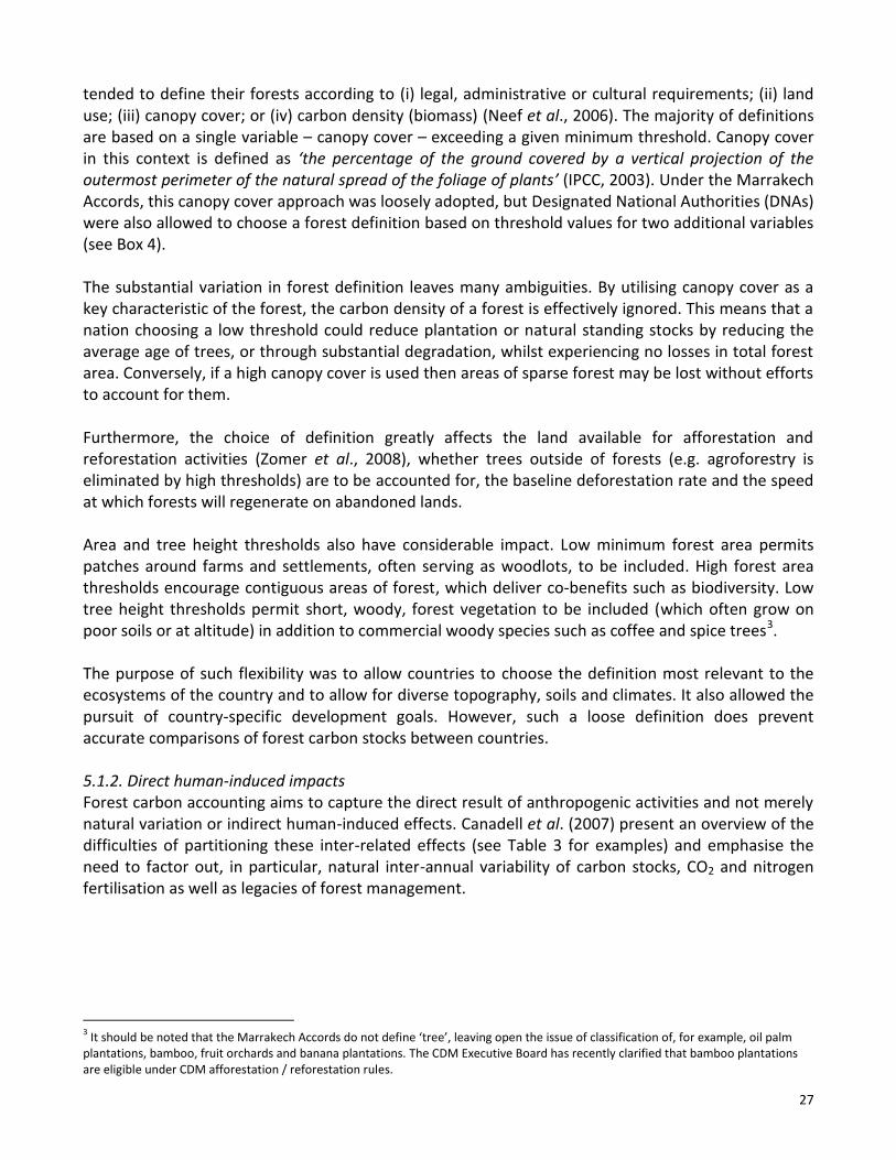
27

tended to define their forests according to (i) legal, administrative or cultural requirements; (ii) land use; (iii) canopy cover; or (iv) carbon density (biomass) (Neef et al., 2006). The majority of definitions are based on a single variable – canopy cover – exceeding a given minimum threshold. Canopy cover in this context is defined as ‘the percentage of the ground covered by a vertical projection of the outermost perimeter of the natural spread of the foliage of plants’ (IPCC, 2003). Under the Marrakech Accords, this canopy cover approach was loosely adopted, but Designated National Authorities (DNAs) were also allowed to choose a forest definition based on threshold values for two additional variables (see Box 4). The substantial variation in forest definition leaves many ambiguities. By utilising canopy cover as a key characteristic of the forest, the carbon density of a forest is effectively ignored. This means that a nation choosing a low threshold could reduce plantation or natural standing stocks by reducing the average age of trees, or through substantial degradation, whilst experiencing no losses in total forest area. Conversely, if a high canopy cover is used then areas of sparse forest may be lost without efforts to account for them. Furthermore, the choice of definition greatly affects the land available for afforestation and reforestation activities (Zomer et al., 2008), whether trees outside of forests (e.g. agroforestry is eliminated by high thresholds) are to be accounted for, the baseline deforestation rate and the speed at which forests will regenerate on abandoned lands. Area and tree height thresholds also have considerable impact. Low minimum forest area permits patches around farms and settlements, often serving as woodlots, to be included. High forest area thresholds encourage contiguous areas of forest, which deliver co-benefits such as biodiversity. Low tree height thresholds permit short, woody, forest vegetation to be included (which often grow on poor soils or at altitude) in addition to commercial woody species such as coffee and spice trees3. The purpose of such flexibility was to allow countries to choose the definition most relevant to the ecosystems of the country and to allow for diverse topography, soils and climates. It also allowed the pursuit of country-specific development goals. However, such a loose definition does prevent accurate comparisons of forest carbon stocks between countries. 5.1.2. Direct human-induced impacts Forest carbon accounting aims to capture the direct result of anthropogenic activities and not merely natural variation or indirect human-induced effects. Canadell et al. (2007) present an overview of the difficulties of partitioning these inter-related effects (see Table 3 for examples) and emphasise the need to factor out, in particular, natural inter-annual variability of carbon stocks, CO2 and nitrogen fertilisation as well as legacies of forest management.

3 It should be noted that the Marrakech Accords do not define ‘tree’, leaving open the issue of classification of, for example, oil palm

plantations, bamboo, fruit orchards and banana plantations. The CDM Executive Board has recently clarified that bamboo plantations are eligible under CDM afforestation / reforestation rules.

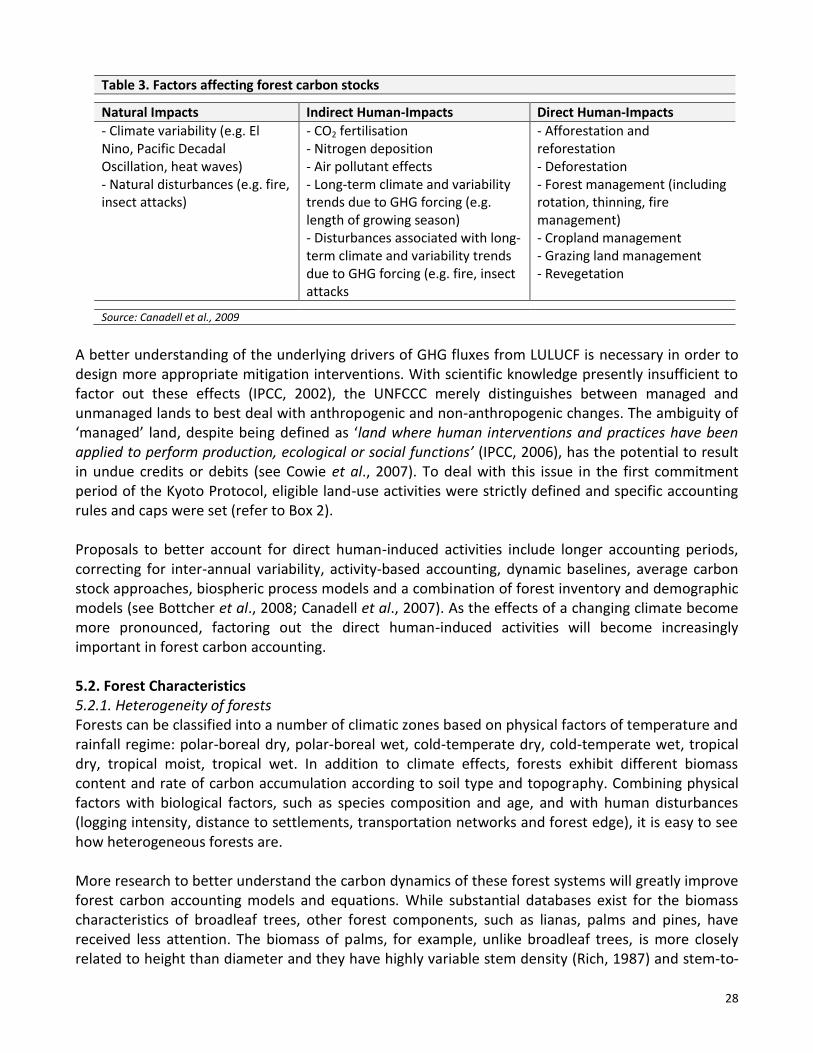
28

Table 3. Factors affecting forest carbon stocks

Natural Impacts Indirect Human-Impacts Direct Human-Impacts - Climate variability (e.g. El Nino, Pacific Decadal Oscillation, heat waves) - Natural disturbances (e.g. fire, insect attacks)

- CO2 fertilisation - Nitrogen deposition - Air pollutant effects - Long-term climate and variability trends due to GHG forcing (e.g. length of growing season) - Disturbances associated with long-term climate and variability trends due to GHG forcing (e.g. fire, insect attacks

- Afforestation and reforestation - Deforestation - Forest management (including rotation, thinning, fire management) - Cropland management - Grazing land management - Revegetation

Source: Canadell et al., 2009

A better understanding of the underlying drivers of GHG fluxes from LULUCF is necessary in order to design more appropriate mitigation interventions. With scientific knowledge presently insufficient to factor out these effects (IPCC, 2002), the UNFCCC merely distinguishes between managed and unmanaged lands to best deal with anthropogenic and non-anthropogenic changes. The ambiguity of ‘managed’ land, despite being defined as ‘land where human interventions and practices have been applied to perform production, ecological or social functions’ (IPCC, 2006), has the potential to result in undue credits or debits (see Cowie et al., 2007). To deal with this issue in the first commitment period of the Kyoto Protocol, eligible land-use activities were strictly defined and specific accounting rules and caps were set (refer to Box 2). Proposals to better account for direct human-induced activities include longer accounting periods, correcting for inter-annual variability, activity-based accounting, dynamic baselines, average carbon stock approaches, biospheric process models and a combination of forest inventory and demographic models (see Bottcher et al., 2008; Canadell et al., 2007). As the effects of a changing climate become more pronounced, factoring out the direct human-induced activities will become increasingly important in forest carbon accounting. 5.2. Forest Characteristics 5.2.1. Heterogeneity of forests Forests can be classified into a number of climatic zones based on physical factors of temperature and rainfall regime: polar-boreal dry, polar-boreal wet, cold-temperate dry, cold-temperate wet, tropical dry, tropical moist, tropical wet. In addition to climate effects, forests exhibit different biomass content and rate of carbon accumulation according to soil type and topography. Combining physical factors with biological factors, such as species composition and age, and with human disturbances (logging intensity, distance to settlements, transportation networks and forest edge), it is easy to see how heterogeneous forests are. More research to better understand the carbon dynamics of these forest systems will greatly improve forest carbon accounting models and equations. While substantial databases exist for the biomass characteristics of broadleaf trees, other forest components, such as lianas, palms and pines, have received less attention. The biomass of palms, for example, unlike broadleaf trees, is more closely related to height than diameter and they have highly variable stem density (Rich, 1987) and stem-to-

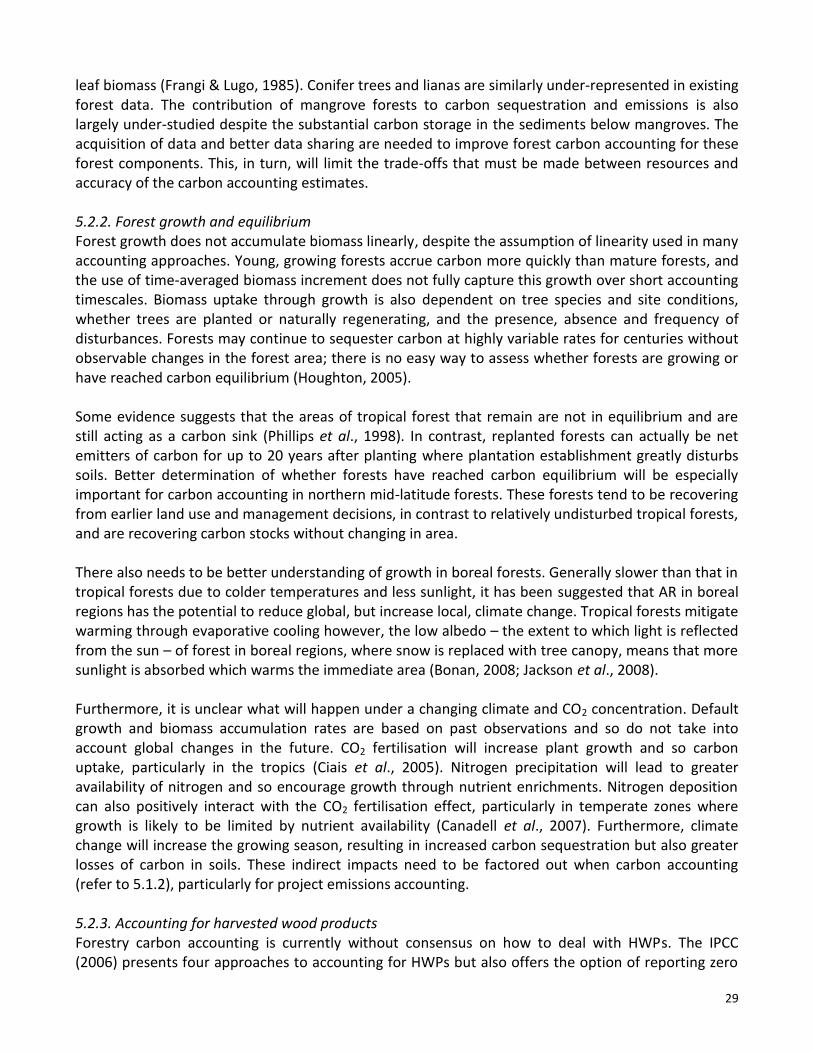
29

leaf biomass (Frangi & Lugo, 1985). Conifer trees and lianas are similarly under-represented in existing forest data. The contribution of mangrove forests to carbon sequestration and emissions is also largely under-studied despite the substantial carbon storage in the sediments below mangroves. The acquisition of data and better data sharing are needed to improve forest carbon accounting for these forest components. This, in turn, will limit the trade-offs that must be made between resources and accuracy of the carbon accounting estimates. 5.2.2. Forest growth and equilibrium Forest growth does not accumulate biomass linearly, despite the assumption of linearity used in many accounting approaches. Young, growing forests accrue carbon more quickly than mature forests, and the use of time-averaged biomass increment does not fully capture this growth over short accounting timescales. Biomass uptake through growth is also dependent on tree species and site conditions, whether trees are planted or naturally regenerating, and the presence, absence and frequency of disturbances. Forests may continue to sequester carbon at highly variable rates for centuries without observable changes in the forest area; there is no easy way to assess whether forests are growing or have reached carbon equilibrium (Houghton, 2005). Some evidence suggests that the areas of tropical forest that remain are not in equilibrium and are still acting as a carbon sink (Phillips et al., 1998). In contrast, replanted forests can actually be net emitters of carbon for up to 20 years after planting where plantation establishment greatly disturbs soils. Better determination of whether forests have reached carbon equilibrium will be especially important for carbon accounting in northern mid-latitude forests. These forests tend to be recovering from earlier land use and management decisions, in contrast to relatively undisturbed tropical forests, and are recovering carbon stocks without changing in area. There also needs to be better understanding of growth in boreal forests. Generally slower than that in tropical forests due to colder temperatures and less sunlight, it has been suggested that AR in boreal regions has the potential to reduce global, but increase local, climate change. Tropical forests mitigate warming through evaporative cooling however, the low albedo – the extent to which light is reflected from the sun – of forest in boreal regions, where snow is replaced with tree canopy, means that more sunlight is absorbed which warms the immediate area (Bonan, 2008; Jackson et al., 2008). Furthermore, it is unclear what will happen under a changing climate and CO2 concentration. Default growth and biomass accumulation rates are based on past observations and so do not take into account global changes in the future. CO2 fertilisation will increase plant growth and so carbon uptake, particularly in the tropics (Ciais et al., 2005). Nitrogen precipitation will lead to greater availability of nitrogen and so encourage growth through nutrient enrichments. Nitrogen deposition can also positively interact with the CO2 fertilisation effect, particularly in temperate zones where growth is likely to be limited by nutrient availability (Canadell et al., 2007). Furthermore, climate change will increase the growing season, resulting in increased carbon sequestration but also greater losses of carbon in soils. These indirect impacts need to be factored out when carbon accounting (refer to 5.1.2), particularly for project emissions accounting. 5.2.3. Accounting for harvested wood products Forestry carbon accounting is currently without consensus on how to deal with HWPs. The IPCC (2006) presents four approaches to accounting for HWPs but also offers the option of reporting zero

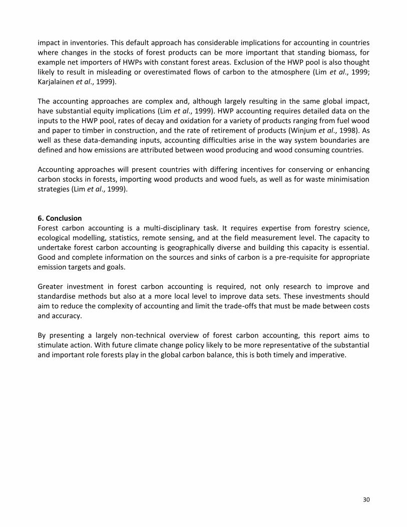
30

impact in inventories. This default approach has considerable implications for accounting in countries where changes in the stocks of forest products can be more important that standing biomass, for example net importers of HWPs with constant forest areas. Exclusion of the HWP pool is also thought likely to result in misleading or overestimated flows of carbon to the atmosphere (Lim et al., 1999; Karjalainen et al., 1999). The accounting approaches are complex and, although largely resulting in the same global impact, have substantial equity implications (Lim et al., 1999). HWP accounting requires detailed data on the inputs to the HWP pool, rates of decay and oxidation for a variety of products ranging from fuel wood and paper to timber in construction, and the rate of retirement of products (Winjum et al., 1998). As well as these data-demanding inputs, accounting difficulties arise in the way system boundaries are defined and how emissions are attributed between wood producing and wood consuming countries. Accounting approaches will present countries with differing incentives for conserving or enhancing carbon stocks in forests, importing wood products and wood fuels, as well as for waste minimisation strategies (Lim et al., 1999). 6. Conclusion Forest carbon accounting is a multi-disciplinary task. It requires expertise from forestry science, ecological modelling, statistics, remote sensing, and at the field measurement level. The capacity to undertake forest carbon accounting is geographically diverse and building this capacity is essential. Good and complete information on the sources and sinks of carbon is a pre-requisite for appropriate emission targets and goals. Greater investment in forest carbon accounting is required, not only research to improve and standardise methods but also at a more local level to improve data sets. These investments should aim to reduce the complexity of accounting and limit the trade-offs that must be made between costs and accuracy. By presenting a largely non-technical overview of forest carbon accounting, this report aims to stimulate action. With future climate change policy likely to be more representative of the substantial and important role forests play in the global carbon balance, this is both timely and imperative.

31

7. Appendices 7.1. Appendix I: ReferencesAchard, F., Eva, H.D., Mayaux, P., Stibig, H.J., Belward, A., 2004. Improved estimates of net carbon emissions from land cover change in the tropics for the 1990s. Global Biogeochemical Cycles, 18, B2008. Andersson, K., Evans, T.P., Richards, K.R., 2009. National forest carbon inventories: policy needs and assessment capacity. Climatic Change, 93, 69-101. Angelsen, A., 2008a. Moving ahead with REDD: issues, options and implications. In: A. Angelsen (ed.) Moving Ahead with REDD: Issues, Options and Implications. Center for International Forestry Research (CIFOR), Bogor, Indonesia. Angelsen, A., 2008b. How do we set the reference levels for REDD payments? In: A. Angelsen (ed.) Moving Ahead with REDD: Issues, Options and Implications. Center for International Forestry Research (CIFOR), Bogor, Indonesia. Aukland, L., Moura Costa, P., Brown, S., 2002. A Conceptual Framework and Its Application for Addressing Leakage: The Case of Avoided Deforestation. Climate Policy, 94, 1–15. Baldocchi, D.D., 2003. Assessing the eddy covariance technique for evaluating carbon dioxide exchange rates of ecosystems: past, present and future. Global Change Biology, 9, 479–492. Bonan, G., 2008. Forests and Climate Change: Forcings, Feedbacks, and the Climate Benefits of Forests. Science, 320, 1444-1449. Bond, I., Grieg-Gran, Wertz-Kanounnikoff, S., Hazlewood, P., Wunder, S., Angelsen, A., 2009. Incentives to sustain forest ecosystem services: A review and lessons for REDD. Natural Resource Issues No. 16. International Institute for Environment and Development, London, UK, with CIFOR, Bogor, Indonesia, and World Resources Institute, Washington D.C., USA.

Bottcher, H., Kurz, W., Freibauer, A., 2008. Accounting of forest carbon sinks and sources sinks and sources under a future climate protocol-factoring out past disturbance and management effects on age-class structure. Environmental Science and Policy, 11, 669-686. Brown, P., Cabarle, B., Livernash, R., 1997. Carbon Counts: Estimating Climate Change mitigation in Forestry Projects. World Resources Institute, Washington DC. Brown, S., 2002. Measuring carbon in forests: current status and future challenges. Environmental Pollution, 116, 363-372. Brown, S., 1997. Estimating Biomass and Biomass Change of Tropical Forests: a Primer. FAO Forestry Paper 134, Rome, Italy. Brown, S., Lim, B., Schlamadinger, B., 1998. Evaluating Approaches for Estimating Net Emissions of Carbon Dioxide from Forest Harvesting and Wood Products. Report of a meeting sponsored by the IPCC held in Dakar, Senegal, 5-7 May, 1998. [Online] Available from: http://www.ipcc-nggip.iges.or.jp/public/mtdocs/pdfiles/dakar.pdf [accessed July 2009] Brown, S. and A. E. Lugo, 1982. The storage and production of organic matter in tropical forests and their role in the global carbon cycle. Biotropica, 14, 161-187. Cairns, M. A., Brown, S., Helmer, E. H., Baumgardner, G. A., 1997. Root biomass allocation in the world’s upland forests. Oecologia, 111, 1-11. Canadell, J. G., Le Qúeré, C., Raupach, M. R., Field, C. B., Buitenhuis, E. T., Ciais, P., Conway, T. J., Gillett, N. P., Houghton, R. A., Marland, G., 2007. Contributions to accelerating atmospheric CO2 growth from economic activity, carbon intensity, and efficiency of natural sinks. Proceedings of the National Academy of Science, 104, 18,866–18,870.

32

Ciais, P., Reichstein, M., Viovy, N., Granier, A., Ogee, J., Allard, V., Aubinet, M., Buchmann, N., Bernhofer, C., Carrara, A., Chevallier, F., De Noblet, N., Friend, A.D., Friedlingstein, P., Grunwald, T., Heinesch, B., Keronen, P., Knohl, A., Krinner, G., Loustau, D., Manca, G., Matteucci, G., Miglietta, F., Ourcival, J.M., Papale, D., Pilegaard, K., Rambal, S., Seufert, G., Soussana, J.F., Sanz, M.J., Schulze, E.D., Vesala, T., Valentini, R., 2005. Europe-wide reduction in primary productivity caused by the heat and drought in 2003. Nature, 437, 529–533. Cowie, A.L., Kirschbaum, M.U.F., Ward, M., 2007. Options for including all lands in a future greenhouse gas accounting framework. Environmental Science Policy, 10, 306–321. Delaney, M., Brown, S., Lugo, A.E., Torres-Lezama, A., Bello Quintero, N., 1998. The quantity and turnover of dead wood in permanent forest plots in six life zones of Venezuela. Biotropica, 30, 2–11. FAO 2006. Global Forest Resources Assessment 2005. FAO Forestry Paper, Report number: 147. Rome, FAO. FAO 2005. FAOSTAT Forestry data. [Online] Available at http://faostat.fao.org/faostat/collections?subset=forestry [accessed July 2009] Forbes, M.S., Raison, R.J., Skjemstad, J.O., 2006. Formation, transformation and transport of black carbon (charcoal) in terrestrial and aquatic ecosystems. Science of The Total Environment, 370 (1), 190-206. Frangi, J. L., Lugo, A. E., 1985. Ecosystem dynamics of a subtropical floodplain forest. Ecological Monographs, 55, 351-369. Gibbs, H.K., Brown, S., Niles, J.O. and Foley J.A., 2007. Monitoring and Estimating Forest Carbon Stocks: Making REDD a reality. Environmental Resource Letters 2, IOP Publishing Ltd, UK. [Online] Available at: www.iop.org/EJ/article/1748-9326/2/4/045023/erl7_4_045023.html [accessed July 2009]

Giest, H.J, Lambin, E.F., 2001. What Drives Tropical Deforestation: A meta-analysis of proximate and underlying causes of deforestation based on subnational case study evidence. LUCC Report Series No. 4, Louvain, Belgium. Grainger, A., 2008. Difficulties in tracking the long-term global trend in tropical forest area. Proceedings of the National Academy of Science. 105 (2), 818-823. Greenhalgh, S., Daviet, F. and Weninger, E., 2006. The Land Use, Land-Use Change, and Forestry Guidance for GHG Project Accounting. The Greenhouse Gas Protocol, World Resources Institute. Houghton, R.A, 2005. Aboveground Forest Biomass and the Global Carbon Balance. Global Change Biology, 11, 945-958. Houghton, J. T., Meira Filho, L. G., Lim, B., Treanton, K., Mamaty, I., Bonduki, Y., Griggs, D. J., Callander, B. A., 1997. Revised 1996 Guidelines for National Greenhouse Gas Inventories. IPCC/OECD/IEA. IPCC 2007. Climate Change 2007: The Physical Science Basis. Contribution of Working Group I to the Fourth Assessment Report of the Intergovernmental Panel on Climate Change [Solomon, S., D. Qin, . Manning, Z. Chen, M. Marquis, K.B.M.Tignor and H.L. Miller (eds.)]. Cambridge University Press, Cambridge, United Kingdom and New York, NY, USA, 996pp. IPCC 2006. Agriculture, forestry and other land use. In: Eggleston, H.S., Buendia, L., Miwa, K., Ngara, T., Tanabe, K. (Eds.), IPCC Guidelines for National Greenhouse Gas Inventories, Prepared by the National Greenhouse Gas Inventories Programme. IGES, Japan. IPCC 2003. Good Practice Guidance for Land Use, land-Use Change and Forestry. Penman, J., Gytarsky, M., Hiraishi, T., Kruger, D., Pipatti, R., Buendia, L., Miwa, K., Ngara, T., Tanabe, K. and Wagner, F. (Eds). Intergovernmental Panel on Climate Change (IPCC), IPCC/IGES, Hayama, Japan.

33

IPCC 2000. Good Practice Guidance and Uncertainty Management in National Greenhouse Gas Inventories. Penman, J., Kruger, D., Galbally, I., Hiraishi, T., Nyenzi, B., Enmanuel, S., Buendia, L., Hoppaus, R., Martinsen, T., Meijer, J., Miwa, K. and Tanabe, K. (Eds). Intergovernmental Panel on Climate Change (IPCC), IPCC/OECD/IEA/IGES, Hayama, Japan. IPCC 1997. Revised 1996 IPCC Guidelines for National Greenhouse Gas Inventories: Volumes 1, 2 and 3. Houghton, J.T., Meira Filho, L.G., Lim, B., Tréanton, K., Mamaty, I., Bonduki, Y., Griggs, D.J. and Callander, B.A. (Eds). Intergovernmental Panel on Climate Change (IPCC), IPCC/OECD/IEA, Paris, France. ISRIC World Inventory of Soil Emission (WISE) Potential Database, ISRIC, 2009. [Online] Available at: http://www.isric.org/UK/About+ISRIC/Projects/Track+Record/WISE.htm [accessed July 2009] Jackson, R.B., Randerson, J.T., Canadell, J.G., Anderson, R.G., Avissar, R., Baldocchi, D.D., Bonan, G.B., Caldeira, K., Diffenbaugh, N.S., Field, C.B., Hungate, B.A., Jobbágy, E.G., Kueppers, L.M., Nosetto, M.D., Pataki, D.E., 2008. Protecting climate with forests. Environmental Research Letters, 3, 044006. Karjalainen, T., Pussinen, A., Kellomäki, S., Mäkipää, R., 1999. Scenarios for the carbon balance of Finnish forests and wood products. Environmental Science and Policy, 2, 165–175. Lal, R., Bruce, J., 1999. The Potential of World Cropland to Sequester Carbon and Mitigate the Greenhouse Effect. Environnental Science and Policy, 2, 177–185. Landsberg, J.J., Waring, R.H., 1997. A generalized model of forest productivity using simplified concepts of radiation-use efficiency, carbon balance and partitioning. Forest Ecol. Manage., 95, 209–228. Larocque, G.R., Bhatti, J.S., Boutin, R., Chertov, O., 2008. Uncertainty analysis in carbon cycle models of forest ecosystems : Research needs and

development of a theoretical framework to estimate error propagation. Ecological Modelling, 219, 400-412. Lehmann, J., 2007. A Handful of Carbon. Nature, 447, 143-144. Lim, B., Brown, S., Schlamadinger, B., 1999. Carbon accounting for forest harvesting and wood products: review and evaluation of different approaches. Environmental Science and Policy 2, 207–216. Lui, G., Han, S., 2009. Long-term management and timely transfer of carbon into wood products help reduce atmospheric carbon. Ecological Modelling, 220, 1719-1723. MacDicken, K., 1997. A Guide to Monitoring Carbon Storage in Forestry and Agroforestry Projects. Winrock International, 1611 N. Kent St., Suite 600, Arlington, VA 22209, USA. Marland, G., Fruit, K., Sedjo, R., 2001. Accounting for sequestered carbon: the question of permanence. Environmental Science and Policy, 4, 259-268. Marland, G., Schlamadinger, B., 1999. The Kyoto Protocol could make a difference for the optimal forest-based CO2 mitigation strategy: some results from GORCAM. Environmental Science and Policy, 2, 111-124. Masera, O., Garza-Caligaris, J.F., Kanninen, M., Karjalainen, T., Liski, J., Nabuurs, G.J., Pussinen, A., de Jong, B.J., 2003. Modelling carbon sequestration in afforestation, agroforestry and forest management projects: the CO2FIX V.2 approach. Ecological Modelling, 164, 177-199. Metherall, A.K., Harding, L.A., Cole, C.V., Parton, W.J., 1993. CENTURY Soil Organic Matter Model Environment Technical Documentation, Agroecosystem Version 4.0, Great Plains System Research Unit, Tech. Rep. No. 4. USDA-ARS, Ft. Collins. Moura-Costa, P., Stuart, M., Pinard, M., Phillips, G., 2000. Issues related to monitoring, verification and

34

certification of forestry-based carbon offset projects. Mitigation and Adaptation Strategies for Global Change. Nabuurs, G.J., Masera, O. Andrasko, K. Benitez-Ponce, P. Boer, R. Dutschke, M. Elsiddig, E. Ford-Robertson, J. Frumhoff, P. Karjalainen, T. Krankina, O. Kurz, W.A. Matsumoto, M. Oyhantcabal, W. Ravindranath, N.H. Sanz Sanchez, M.J. Zhang, X., 2007. Forestry. In Climate Change (2007) Mitigation. Contribution of Working Group III to the Fourth Assessment Report of the Intergovernmental Panel on Climate Change [B. Metz, O.R. Davidson, P.R. Bosch, R. Dave, L.A. Meyer (eds)], Cambridge University Press, Cambridge, United Kingdom and New York, NY, USA Nabuurs, G.J., Garza-Caligaris, J.F., Kanninen, M., Karjalainen, T., Lapvetelainen, T., Liski, J., Masera, O., Mohren, G.M.J., Pussinen, A., Schelhaas, M.J., 2002. CO2FIX V2.0. Manual of a model for quantifying carbon sequestration in forest ecosystems and wood products. ALTERRA Report, The Netherlands. Nabuurs, G. J., M. J. Schelhaas, Pussinen, A., 2000. Validation of the European forest information scenario model (EFISCEN) and a projection of Finnish forests. Silva Fennica 34(2), 167-179. Neef, T., von Luepke, H., Schoene, D., 2006. Choosing a forest definition for the Clean Development Mechanism. Forests and Climate Change Working Paper 4, FAO. Ogle, S.M., Breidt, F.J., Eve, M.D., Paustian, K., 2005. Agricultural management impacts on soil organic carbon storage under moist and dry climatic conditions of temperate and tropical regions. Biogeochemistry, 72, 87-121. Parpia, A. 2007. Avoided Deforestation and the Permanence of Terrestrial Carbon. MSc Thesis at Imperial College London, Centre for Environmental Policy, London. Pearson, T., Walker, S. and Brown, S., 2005. Sourcebook for Land Use, Land-Use Change and

Forestry Projects. Winrock International and the Bio Carbon Fund of the World Bank. Pinard, M. A., Putz., F. E., 1996. Retaining forest biomass by reduced impact logging damage. Biotropica 28, 278-295. Pingoud, K., Schlamadinger, B, Gronkvist, B., Brown, S., Cowie, A., Marland, G., 2004. Approaches for inclusion of harvested wood products in future GHG inventories under the UNFCCC, and their consistency with the overall UNFCCC inventory reporting framework. IEA Bioenergy Task 38: Greenhouse Gas Balances of Biomass and Bioenergy Systems. Phillips, O.L., Malhi, Y., Higuchi, N., Laurance, W.F., Núñez, P.V., Vásquez, R.M., Laurance, S.G., Ferreira, L.V., Stern, M., Brown, S., Grace, J., 1998. Changes in the carbon balance of tropical forests: evidence from long-term plots. Science, 282, 439–442. Rich, P.M., 1987. Mechanical structure of the stem of arborescent palms. Botanical Gazette, 148, 42-50. Richards, G., Evans, D., 2000. Carbon Accounting Model for Forests (CAMFor) Users Manual. National Carbon Accounting System Technical Report No. 26. [Online] Available at: http://www.greenhouse.gov.au/ncas/ [accessed July 2009] Running, S.W., Gower, S.T., 1991. FOREST-BGC, A general model of forest ecosystem processes for regional applications. II. Dynamic carbon allocation and nitrogen budgets. Tree Physiol. 9, 147–160. Sajwaj, T., Harley, M., Parker, C. 2008 Eliasch Review: Forest Managements Impacts on Ecosystem Services, AEA. Schlamadinger, B., Marland, G., 2000. Land Use and Global Climate Change: Forests, Land Management and the Kyoto Protocol. Pew Center on global Climate Change. Schmidt, M.W.I, 2004. Carbon budget in the black. Nature; 427, 305-306.

35

Schwarze, R., Niles, J.O., Olander., J., 2002. Understanding and Managing Leakage in Forest-Based Greenhouse-Gas-Mitigation Projects. London: Royal Society. Sedjo, R., Marland, G., 2003. Inter-trading Permanent Emissions Credits and Rented Temporary Carbon Emissions Offsets: Some Issues and Alternatives. Climate Policy, 3, 435-444. Sohngen, B., Brown, S., 2004. Measuring Leakage from Carbon Projects in Open Economies: A Stop Timber Harvesting Project in Bolivia as a Case Study. Canadian Journal of Forestry Research, 34 (11), 669-674. Stern, N., 2006. The Economics of Climate Change: The Stern Review. Cambridge University Press, Cambridge, UK.

UN-REDD, 2008. Role of satellite remote sensing in REDD. Issues paper. UN-REDD Programme. Working paper 1. Oct 2008. Voluntary Carbon Standard (VCS) 2008. Guidance for Agriculture, Forestry and other land Use Projects. VCS Association. Westlake, D.F., 1966. The biomass and productivity of glyceria maxima: I. Seasonal changes in biomass. Journal of Ecology, 54, 745-753. Winjum, J.K., Brown, S., Schlamadinger, B., 1998. Forest harvests and wood products: sources and sinks of atmospheric carbon dioxide. Forest Science, 44, 272-284. Zomer, R.J., Trabucco, A., Verchot, L.V., Muys, B., 2008. Land Area Eligible for Afforestation and Reforestation within the CDM: A Global Analysis of the Impact of forest definition. Mitigation and Adaptation Strategies, Global Change, 13, 219-239.

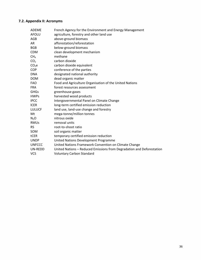
36

7.2. Appendix II: Acronyms

ADEME French Agency for the Environment and Energy Management AFOLU agriculture, forestry and other land use AGB above-ground biomass AR afforestation/reforestation BGB below-ground biomass CDM clean development mechanism CH4 methane CO2 carbon dioxide CO2e carbon dioxide equivalent COP conference of the parties DNA designated national authority DOM dead organic matter FAO Food and Agriculture Organisation of the United Nations FRA forest resources assessment GHGs greenhouse gases HWPs harvested wood products IPCC Intergovernmental Panel on Climate Change lCER long-term certified emission reduction LULUCF land use, land-use change and forestry Mt mega-tonne/million tonnes N2O nitrous oxide RMUs removal units RS root-to-shoot ratio SOM soil organic matter tCER temporary certified emission reduction UNDP United Nations Development Programme UNFCCC United Nations Framework Convention on Climate Change UN-REDD United Nations – Reduced Emissions from Degradation and Deforestation VCS Voluntary Carbon Standard

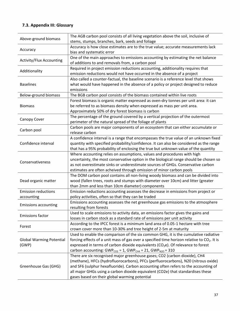
37

7.3. Appendix III: Glossary

Above-ground biomass The AGB carbon pool consists of all living vegetation above the soil, inclusive of stems, stumps, branches, bark, seeds and foliage

Accuracy Accuracy is how close estimates are to the true value; accurate measurements lack bias and systematic error

Activity/Flux Accounting One of the main approaches to emissions accounting by estimating the net balance of additions to and removals from, a carbon pool

Additionality Required in project emission reductions accounting, additionality requires that emission reductions would not have occurred in the absence of a project

Baselines Also called a counter-factual, the baseline scenario is a reference level that shows what would have happened in the absence of a policy or project designed to reduce emissions

Below-ground biomass The BGB carbon pool consists of the biomass contained within live roots

Biomass Forest biomass is organic matter expressed as oven-dry tonnes per unit area: it can be referred to as biomass density when expressed as mass per unit area. Approximately 50% of dry forest biomass is carbon

Canopy Cover The percentage of the ground covered by a vertical projection of the outermost perimeter of the natural spread of the foliage of plants

Carbon pool Carbon pools are major components of an ecosystem that can either accumulate or release carbon

Confidence interval A confidence interval is a range that encompasses the true value of an unknown fixed quantity with specified probability/confidence. It can also be considered as the range that has a 95% probability of enclosing the true but unknown value of the quantity

Conservativeness

Where accounting relies on assumptions, values and procedures with high uncertainty, the most conservative option in the biological range should be chosen so as not overestimate sinks or underestimate sources of GHGs. Conservative carbon estimates are often acheived through omission of minor carbon pools

Dead organic matter The DOM carbon pool contains all non-living woody biomass and can be divided into wood (fallen trees, roots and stumps with diameter over 10cm) and litter (greater than 2mm and less than 10cm diameter) components

Emission reductions accounting

Emission reductions accounting assesses the decrease in emissions from project or policy activities, often so that they can be traded

Emissions accounting Emissions accounting assesses the net greenhouse gas emissions to the atmosphere resulting from forests

Emissions factor Used to scale emissions to activity data, an emissions factor gives the gains and losses in carbon stock as a standard rate of emissions per unit activity

Forest According to the IPCC forest is a minimum land area of 0.05-1 hectare with tree crown cover more than 10-30% and tree height of 2-5m at maturity

Global Warming Potential (GWP)

Used to enable the comparison of the six common GHG, it is the cumulative radiative forcing effects of a unit mass of gas over a specified time horizon relative to CO2. It is expressed in terms of carbon dioxide equivalents (CO2e). Of relevance to forest carbon accounting: GWPCO2 = 1, GWPCH4 = 21, GWPN2O = 310

Greenhouse Gas (GHG)

There are six recognised major greenhouse gases; CO2 (carbon dioxide), CH4 (methane), HFCs (hydrofluorocarbons), PFCs (perfluorocarbons), N20 (nitrous oxide) and SF6 (sulphur hexafluoride). Carbon accounting often refers to the accounting of all major GHGs using a carbon dioxide equivalent (CO2e) that standardises these gases based on their global warming potential

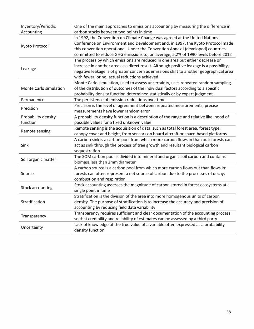
38

Inventory/Periodic Accounting

One of the main approaches to emissions accounting by measuring the difference in carbon stocks between two points in time

Kyoto Protocol

In 1992, the Convention on Climate Change was agreed at the United Nations Conference on Environment and Development and, in 1997, the Kyoto Protocol made this convention operational. Under the Convention Annex I (developed) countries committed to reduce GHG emissions to, on average, 5.2% of 1990 levels before 2012

Leakage

The process by which emissions are reduced in one area but either decrease or increase in another area as a direct result. Although positive leakage is a possibility, negative leakage is of greater concern as emissions shift to another geographical area with fewer, or no, actual reductions achieved

Monte Carlo simulation Monte Carlo simulation, used to assess uncertainty, uses repeated random sampling of the distribution of outcomes of the individual factors according to a specific probability density function determined statistically or by expert judgment

Permanence The persistence of emission reductions over time

Precision Precision is the level of agreement between repeated measurements; precise measurements have lower random error

Probability density function

A probability density function is a description of the range and relative likelihood of possible values for a fixed unknown value

Remote sensing Remote sensing is the acquisition of data, such as total forest area, forest type, canopy cover and height, from sensors on board aircraft or space-based platforms

Sink A carbon sink is a carbon pool from which more carbon flows in than out: forests can act as sink through the process of tree growth and resultant biological carbon sequestration

Soil organic matter The SOM carbon pool is divided into mineral and organic soil carbon and contains biomass less than 2mm diameter

Source A carbon source is a carbon pool from which more carbon flows out than flows in: forests can often represent a net source of carbon due to the processes of decay, combustion and respiration

Stock accounting Stock accounting assesses the magnitude of carbon stored in forest ecosystems at a single point in time

Stratification Stratification is the division of the area into more homogenous units of carbon density. The purpose of stratification is to increase the accuracy and precision of accounting by reducing field data variability

Transparency Transparency requires sufficient and clear documentation of the accounting process so that credibility and reliability of estimates can be assessed by a third party

Uncertainty Lack of knowledge of the true value of a variable often expressed as a probability density function

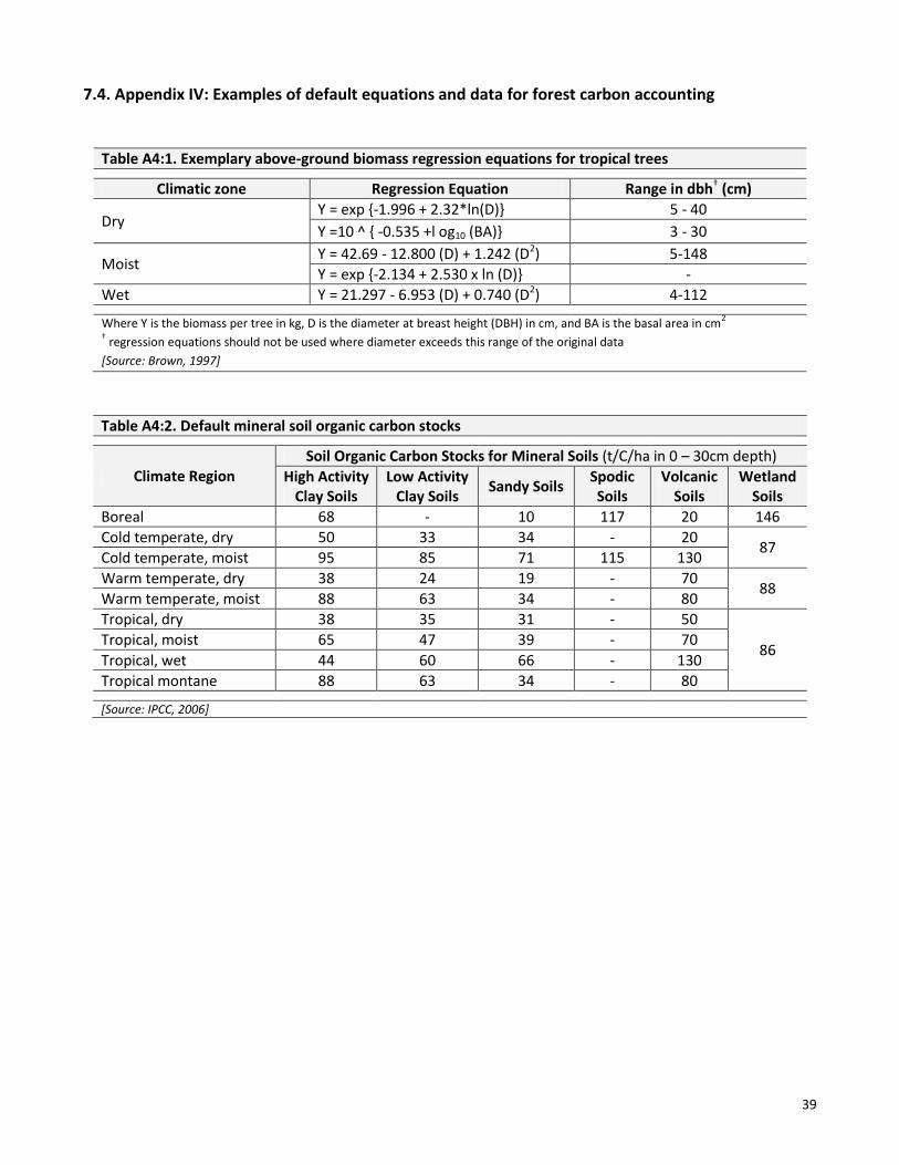
39

7.4. Appendix IV: Examples of default equations and data for forest carbon accounting

Table A4:1. Exemplary above-ground biomass regression equations for tropical trees

Climatic zone Regression Equation Range in dbh† (cm)

Dry Y = exp {-1.996 + 2.32*ln(D)} 5 - 40

Y =10 ^ { -0.535 +l og10 (BA)} 3 - 30

Moist Y = 42.69 - 12.800 (D) + 1.242 (D2) 5-148 Y = exp {-2.134 + 2.530 x ln (D)} -

Wet Y = 21.297 - 6.953 (D) + 0.740 (D2) 4-112

Where Y is the biomass per tree in kg, D is the diameter at breast height (DBH) in cm, and BA is the basal area in cm2

† regression equations should not be used where diameter exceeds this range of the original data

[Source: Brown, 1997]

Table A4:2. Default mineral soil organic carbon stocks

Climate Region Soil Organic Carbon Stocks for Mineral Soils (t/C/ha in 0 – 30cm depth)

High Activity Clay Soils

Low Activity Clay Soils

Sandy Soils Spodic Soils

Volcanic Soils

Wetland Soils

Boreal 68 - 10 117 20 146 Cold temperate, dry 50 33 34 - 20

87 Cold temperate, moist 95 85 71 115 130 Warm temperate, dry 38 24 19 - 70

88 Warm temperate, moist 88 63 34 - 80 Tropical, dry 38 35 31 - 50

86 Tropical, moist 65 47 39 - 70 Tropical, wet 44 60 66 - 130 Tropical montane 88 63 34 - 80

[Source: IPCC, 2006]

40

CDM Capacity Development in Eastern and Southern Africa